the dynamics of price dispersion, or edgeworth variations
TRANSCRIPT

The Dynamics of Price Dispersion,
or Edgeworth Variations
Timothy Cason Department of Economics, Purdue University
Daniel Friedman
Department of Economics, UCSC
and
Florian Wagener CeNDEF, University of Amsterdam
March 24, 2003
Abstract:
Hypotheses on the dynamics of dispersed prices are extracted from computer simulations,
as well as traditional and recent theory. The hypotheses are tested on existing laboratory data.
As predicted in some variations of the Edgeworth hypothesis, the laboratory data exhibit a
significant cycle. Relative to the unique stationary distribution, the empirical distribution of
posted prices has excess mass in an interval that moves downward over time until it approaches
the lower boundary of the stationary distribution. Then the excess mass jumps upward and the
downward cycle resumes. The amplitude of the cycle seems fairly constant over the longer
experimental sessions. Of the simulations we consider, the one closest to Edgeworth’s 1925
account, a hybrid of gradient dynamics and logit dynamics, seems to best reproduce the observed
dynamics.
Acknowledgements: Financial support for the laboratory data collection was provided by the NSF under grants SBR-9617917 and SBR-9709874. We are grateful to Ed Hopkins and Jörgen Weibull for helpful discussions, and to two anonymous referees for thoughtful comments. The second author thanks CeNDEF for sponsoring the 2002 Workshop on Economic Dynamics
2
where the idea for this paper emerged, and thanks Harvard Experimental Economics Lab for hospitality as the paper came together. The third author was supported under the CeNDEF Pioneer grant of the Netherlands Organization for Science (NWO).

The Dynamics of Price Dispersion
1. Introduction
The law of one price fails dramatically even in Internet markets where it should have its best shot
(e.g., Baye and Morgan, 2001; Pauly, Herring and Song, 2002). This observation renews interest
in theoretical debates on price dynamics and price dispersion that go back at least to Bertrand
(1883) and Edgeworth (1925).
Bertrand argued for a unified competitive price, noting that at any higher price at least
one seller could substantially increase sales volume and profit by slightly decreasing his price.
Edgeworth argued that the outcome is more complicated when the sellers have binding capacity
constraints at the competitive price. He predicted a price cycle in which sellers reduce price in
small increments when there is excess capacity, but jump to much higher prices when the
capacity constraints bind. Maskin and Tirole (1988) consider a duopoly with alternating moves
(and no capacity constraints) and obtain price cycles as Markov perfect equilibria.
Modern textbook treatments of multi-firm oligopolies (e.g., Tirole, 1988) downplay price
dynamics and instead focus on stationary price dispersion, supported as a mixed strategy Nash
equilibrium. In particular, the Burdett and Judd (1983) noisy search model has a unique Nash
equilibrium price distribution, denoted NSE below. The distribution is truly dispersed—i.e., it
has positive density over a non-trivial range of prices—for most parameter values of the buyer
search technology, but for extreme parameter values the distribution degenerates to a unified
competitive price or to a unified monopoly price.
Hopkins and Seymour (2002) show that the unified monopoly price NSE is dynamically
stable but that all relevant dispersed price equilibria are unstable under a wide class of learning
dynamics. Their analysis leaves open the question of what behavior we should then observe. The

2
possibilities include convergence to a unified price, or small or large amplitude cycles in the
price distribution, or chaos.
In this paper we further analyze laboratory data originally gathered to investigate NSE.
After offering more details on the theory, we describe a set of dynamic computer simulations of
the dispersed prices, and derive testable hypotheses. Then we present the laboratory procedures
and data. The data feature dispersed prices that tend to cycle. Estimated transition rates among
the quartiles of the empirical price distribution confirm an Edgeworth-like cycle. The amplitude
of the cycle is not small, and does not appear to decrease over time. Of the simulations we
consider, a hybrid of gradient dynamics and logit dynamics seems to best reproduce the observed
dynamics.
2. Theory
A textbook account of Edgeworth dynamics (Chamberlin, 1962, includes a classic example)
typically begins by describing Bertrand best reply dynamics in a symmetric oligopoly with
negligible fixed costs and constant marginal cost. Each period each firm posts a price slightly
below the prices posted in the previous period. Eventually prices decline to the firms’ marginal
cost and profit is zero. The account then recalls Edgeworth’s observation that if demand at this
low price exceeds the firms’ combined capacity, then a firm’s best response is to charge the
monopoly price for the residual demand. Other firms follow, Bertrand competition resumes, and
a new price cycle begins.
We shall refer to the foregoing as the basic Edgeworth cycle (BEC) and, somewhat
exaggerating its precision, we shall say that its observable features are a narrow interval of
prices each period that moves downward until it hits bottom, then jumps upward, with cycles of

3
constant amplitude and frequency.
Modern discussions such as Tirole (1988) question whether such a BEC is an
equilibrium, and focus on mainly on stationary equilibrium distributions. The relevant
equilibrium in the present context is the Burdett and Judd (1983) Noisy Search Equilibrium
distribution (NSE), derived in closed form in Cason and Friedman (2003). The presumption
seems to be that if cycles were to occur, their amplitude would decrease over time and the
distribution would converge to NSE.
Hopkins and Seymour (2002) reverse this presumption. They show that NSE is
dynamically unstable under a wide class of learning dynamics. The local linear approximation
indicates that a small perturbation of NSE will lead to Edgeworth-like cycles whose amplitude is
small at first but increasing. They refer to the cycles as Rock-Paper-Scissors (RPS) to emphasize
that an excess of medium prices follows an excess of high prices that follows an excess of low
prices that follows an excess of medium prices, in the same way that, in the familiar children’s
game, Paper beats Rock which beats Scissors which beats Paper. Their analysis does not show
whether the cycle amplitude tapers off at some moderate level (i.e., the attractor is a stable limit
cycle not far from the NSE distribution), or diverges to a high amplitude BEC, or goes chaotic.
The simulations introduced below demonstrate that the answer depends on the specific dynamics
and parameters.
The simulations represent buyers via an algorithm that is derived from the Noisy Search
assumption that each of a continuum of buyers (total mass normalized to 1) seeks to buy a unit at
lowest price, and employs an optimal reservation price search strategy given a search technology
that produces random samples of sellers’ posted prices. The initial sample contains one price
with probability q≥0 or two prices with probability 1- q≥0, and the buyer can obtain a fresh such
4
sample at cost c≥0. When the distribution of posted prices has cumulative distribution function
F, a seller posting price p will then obtain sales volume s(p) = q + 2(1- q)(1-F(p)) if p ≤ p* =
c/(1-q) and s(p) = 0 if p > p*. The algorithm yields seller profits π = ps(p) because production
cost is normalized to 0. NSE in this setup is characterized by an equilibrium price dispersion
with distribution function F(p) = q
qp
p22
*11−
−+ on the support interval [qp*/(2-q), p*].
This distribution comes from an equal profit condition and is nontrivial when c > 0 and 0<q<1;
see Cason and Friedman (2003) for the derivations.
2.1 Gradient dynamics.
Consider now what happens away from NSE. One possibility is that sellers each period consider
nearby prices and (with some inertia) chose those that would have been most profitable last
period.
We simulate these gradient dynamics by choosing a price grid 0 ≤ p1≤ …≤pi ≤ …≤ pn ,
initial proportions of sellers f1, …, fi , …, fn posting these prices, and a positive adjustment rate
parameter α. The simulation computes profit πi as above at each price pi, and then adjusts the
proportion of sellers as follows. For each price pi,
(1) if πi-1 > πi then fi decreases and fi-1 increases by the amount (πi-1 - πi) α fi; and
if πi-1 < πi then fi increases and fi-1 decreases by the amount (πi - πi-1) α fi-1.
The index i here is to be understood mod n, so that p1 and pn are adjacent.1 The idea is that the
probability mass describing sellers’ choices moves between nearest neighbors, up the profit
1 That is, the highest relevant price p* is deemed nearby to the lowest relevant price qp*/(2-q). Thus we avoid imposing an arbitrary treatment of endpoints, e.g., as absorbing or reflecting. More importantly, thus we allow the possibility of rapid transitions from low to high prices, as hypothesized in the Edgeworth (or RPS) story.

5
gradient. The flux is proportional to the slope of the gradient and to the mass already there.
These dynamics do not satisfy the hypotheses of Hopkins and Seymour’s theorem, so we
have no theoretical prediction regarding their convergence behavior. Simulations therefore are
especially helpful.
Figure 1A shows a typical simulation. From an initial uniform distribution, the density
evolves via heavily damped RPS oscillations to a neighborhood of the NSE distribution. But it
seems to converge to a low amplitude limit cycle rather than to the NSE, and the Figure shows
the initial part of such a cycle. Behavior is qualitatively the same for other buyer parameters c >
0 and 0 < q < 1. Figure 1B shows that as the price grid gets finer, the time average distribution
converges very closely to the NSE distribution.
Figure 1A [dyn_supp2.pdf ]about here
Figure 1B [conv_2.pdf] about here
2.2. Replicator dynamics
Replicator dynamics (Taylor and Jonker, 1978; Weibull, 1995) are perhaps the most widely
known adjustment processes. They do satisfy the assumptions of Hopkins and Seymour's
theorem so we do not expect convergence to NSE. Our simulation uses the same price grid and
profit calculations as before, notes the current average profit πA = Σifiπi , and computes the next
period proportions fi' from
(2) fi' = fi + ((πi -πA )/πA )α fi.
That is, probability mass moves to or from any price point at a rate proportional to its payoff
(relative to the population average) and to the mass already there.
6
Figure 2A shows a typical replicator simulation. From an initial uniform distribution, the
density quickly diverges via increasing RPS oscillations to an extreme basic Edgeworth cycle
(BEC). Figure 2B shows that the time-averaged distribution does not converge to NSE, but rather
to something closer to the uniform distribution (but with moderate skew in the same direction as
NSE.)
Figure 2A [dyn_supp1.pdf ]about here
Figure 2B [conv_1.pdf] about here
.
2.3. Logit dynamics
In the case of replicator dynamics, prices are coupled only through the average profit. For our
logit dynamics, coupling between two price levels is more explicit. Using the same price grid
and profit calculations as before, compute the “attraction weights” βi each period from
Note that βi is close to its maximum value α if the profit is uniquely maximized at price pi and βi
is close to its minimum value 0 if the profit at pi is much lower than the maximum. Note also that
larger values of the parameter λ create larger differences in βi for given profit differentials.
However, it turned out that our final results hardly depended on λ. To reduce the number of free
parameters, we set it equal to unity.
The dynamics are now specified as follows: for every pair of prices pi and pj, each period
(3) a portion βi fj of the sellers at price pj moves to pi, and
a portion βj fi of the sellers at price pi moves to pj.
,∑
=j
i j
i
ee
λπ
λπ
αβ .1 ni ≤≤
7
Simulations show that the dynamics depend more strongly on the adjustment rate α than in the
two previous cases: if α is small, logit dynamics converge to a stationary distribution but one
which is different from the NSE. For larger values of α,2 the stationary distribution becomes
dynamically unstable and cycling behavior is observed. The period of the cycles is much shorter
than in replicator dynamics.
Figures 3A,B about here.
[dyn_supp3.pd , conv_3.pdf]
2.4. Hybrid dynamics
A close reading of Edgeworth3 shows that he allowed transitions to high prices from medium
low as well as from very low prices. To investigate the implications, we constructed a ‘hybrid’
type of dynamics by adding logit-like terms ∑∑≠≠
−ji
ijij
ji ff ββ to the gradient dynamics (1), thus
allowing flux between all possible points of our price grid. For small α, this Edgeworth variation
seems to converge to something resembling NSE, but again it produces fairly large amplitude
cycles for larger values of α, as can be seen in Figure 4A. As the price grid gets finer, the time
averages again converge to a distribution more moderately skewed than the NSE.
Figures 4A, B about here
2.5. Testable Hypotheses
2 Given our choice of price grid etc, the critical value of α is about 0.15. 3 For at every stage in the fall of the price, and before it has reached its limiting value [...], it is competent to each monopolist to deliberate whether it will pay him better to lower the price against his rival [...] or rather to raise it to a higher [...] level [...]. Edgeworth (1925)
8
Let Qit, i=1…4, be the observed fraction of sellers posting prices in quartile i, and let M = ((mij))
be the 4×4 matrix of observed proportions of sellers moving from quartile i one period to quartile
j the next period. We will examine the following hypotheses.
H0: The transition matrix is uniform: all off-diagonal entries equal, and diagonal entries
equal. That is, up to sampling error, mij = mkl for all i≠j and all k≠l; and similarly mii = mjj for all
i,j = 1, …,4. This hypothesis is consistent with NSE equilibrium and with rational expectations,
as well as with no structure.
H1. Bertrand/RPS/Edgeworth cycles: The subdiagonal entries (those representing
transitions to next lower quartile) are significantly larger than other off-diagonal entries. That is,
up to sampling error, mi,i-1 > mij for all j≠i, i-1 for i = 2, 3, 4. This is the clearest implication of
the cycle stories.
H1′. Full cycles: In addition to H1, it is also true that transitions from the lowest quartile
are most often to the highest quartile. That is, m1,4 > m1,j for j =2,3. This is the simplest way of
completing an Edgeworth-like cycle.
H2. Anticipatory dynamics: The sub-subdiagonal entries are larger than the next lower
entries. That is, m4,2 > m4,1. Sellers who anticipate that other sellers respond as in H1 will best
respond with larger price reductions.
H3. Divergence from NSE: H1 holds more strongly in later periods than in early periods.
H4. Convergence to NSE: H1 holds more strongly in earlier periods and H0 holds in later
periods.
3. The Laboratory Experiment
The laboratory experiment used an electronic posted offer market institution with human subjects

9
as sellers and (in the data analyzed below) automated buyers. Subjects were recruited from
undergraduate classes in Economics and Biology at UCSC and Purdue, and were instructed
orally and in writing. The written instructions appear in Cason and Friedman (1999) and are
posted at http://www.mgmt.purdue.edu/faculty/cason/papers/NSEinst.pdf. At the end of the
session the subjects received total profits, converted from lab dollars into U.S. dollars at a fixed
exchange rate and averaging about $20 for sessions that lasted about 90-100 minutes.
Each period each of six sellers posts a single price. Profit π = ps(p) is computed using the
formula given earlier. Sales volume is explained to subjects in terms of the equivalent expression
s(p) = q + 2(1- q)(ri-1)/(n-1), where ri is the rank of a given seller’s price pi among the n≤6
sellers currently posting prices at or below the reservation price p*. For example, with c=0.60
and q=1/3, the reservation price is p* = $0.90; we tell the sellers that each of hundreds of small
automated buyers immediately accepts the lowest price it sees if it is below $0.91 and otherwise
keeps searching, with the result that sales volume will be 0.33 + 1.33(ri-1)/5 if all 6 sellers post
prices below $0.91. The current values of c and q, and corresponding reservation prices, are
shown on the blackboard and on subjects’ screens. At the end of the period each seller see a
sorted list of all posted prices, with corresponding sales volumes and profits. Seller identities are
not shown.
We report here results from four sessions, each divided into several runs of 20-30
consecutive periods in which all treatments are held constant. The treatments include the four
combinations of search cost, c=0.20 or 0.60, and sample size, q = 1/3 or 2/3. Two sessions with
experienced subjects, one with c = 0.20 and one with c = 0.60, were conducted at UCSC; each
included two runs with q = 1/3 and two runs with q = 2/3. Two other sessions, one at Purdue
University with c = 0.20 and the other at UCSC with c = 0.60, used inexperienced subjects and

10
contained one run each with q = 1/3 and q = 2/3. All four sessions had initial runs (not analyzed
here) with q = 1 and q = 0; these values theoretically produce unified price. See Cason and
Friedman (2003) for a more complete description of the experiment, which included additional
sessions with human buyers and with noisier buyer algorithms.
4. Empirical results
We begin by presenting the overall price distributions and the trends in some sample periods.
Different readers may form differing impressions from these qualitative summaries, so we then
proceed to estimate transition matrices and to test our hypotheses.

11
4.1. Price distributions and trends
The equilibrium distribution of posted prices (NSE) shifts up with increases in the probability
that buyers observe only one price (q) and with increases buyer search costs (c), as indicated by
the lighter histogram bars in Figure 5. With 20-cent search costs, NSE prices range between 6
and 30 cents for q=1/3 and range between 30 and 60 cents for q=2/3. With 60-cent search costs,
NSE prices range between 18 and 90 cents for q=1/3 and range between 90 and 180 cents for
q=2/3. The observed distributions, indicated by darker bars, shift as predicted and generally are
in the predicted range. But they tend to be less skewed than the NSE distributions. Cason and
Friedman (2003) offer a detailed analysis of these regularities.
Our present focus is price dynamics. Figures 6 through 8 present the dynamics in a
sample of 3 of the 12 runs studied here. The circles represent posted prices, and the short dashed
line indicates the mean transaction price for each period. Solid vertical lines separate trading
periods, and the horizontal dashed lines indicate the NSE price range.
Figure 6 presents a q=2/3 run with 20-cent search costs. Prices decline gradually in the
first part of the run before they jump up toward the reservation price around period 80. Price
dispersion decreases in the middle of this run before increasing again—reflecting many price
reductions—in later periods. Figure 7 presents a q=1/3 run with 60-cent search costs that begins
with one of the best basic Edgeworth cycles (BEC) we have seen in the data. By contrast, Figure
8 (a q=2/3 run with 60-cent search costs) shows prices with higher cross-sectional variance; the
distribution shifts down in early periods but seems to stablize in later periods.
4.2. Transition matrices
The analysis begins with the empirical distribution of posted prices Fk, where k indexes the

12
experimental treatment (i.e., the search cost c and probability q of receiving only one seller’s
price).4 First, define the quartile cutoff points r1k, r2k and r3k, where 0.25 = Fk(r1k), 0.50 = Fk(r2k),
and 0.75 = Fk(r3k). Then define the four quartiles as the price observation between the cutoff
points. Those between r1k and r2k, for example, are in quartile 2 (denoted Q2).
The movement of prices from one period to the next can be summarized by a 4×4
transition matrix Mk, where the ijth entry gives the empirical proportion of sellers whose prices
move from quartile i in period t to quartile j in period t+1. Large entries on the diagonal indicate
a stable price distribution and very little churning within the distribution.
Table 1 presents the estimated transition matrices for sessions with experienced subjects,
and Table 2 does the same for inexperienced subjects. Of course, in all the calculations the first
transition from the previous treatment k is excluded. The diagonal entries indicate that prices
remain in the same quartile for two consecutive periods roughly 40 to 75 percent of the time. The
subdiagonal entries indicate that transitions to the next lower quartile typically are more frequent
than transitions to any other quartile. The only exceptions are the Q3 quartile in the c=20 and
q=2/3 treatment in Table 1 and the Q4 quartile in the c=20 and q=1/3 treatment in Table 2. In
many cases these transitions are twice as common as any other transition.
Tables 3 and 4 subdivide the experienced subject data into first and second runs. Both
relevant sessions featured a first run of 30 periods and a second run of 20 periods for both q
treatments, so this is a natural way to divide the data. The tables suggest several regularities.
First, particularly for the c=20, q=2/3 and c=60, q=1/3 treatments, the diagonal entries tend to be
higher in the early periods. Of the 16 pairwise diagonal comparisons between Tables 3 and 4 the
values are lower in early periods for only four cases. Second, the subdiagonal entries tend to be 4 The NSE distribution could be used instead of the empirical distribution, but it turns out to be impractical because its lowest quartile contains very few observations. The reason, as documented in the previous subsection, is that the empirical price distributions do not exhibit the strong skewness of the NSE distributions.

13
larger for the late data, except for the c=60, q=1/3 treatment. Indeed, these entries are at least
twice as great as the next highest off diagonal entry in 7 out of the 12 possible rows in the late
period data, compared to only 4 out of the 12 rows in the early period data. Finally, we note a
possible regularity not considered in our list of hypotheses. The transition 4tQ → 1
1tQ + from very
high to very low prices is small for all treatments in the early periods. But this transition is the
most frequent for search cost=60 in the late periods. But this could be an artifact of the small
sample size for 4tQ in the late data, since the number of seller price changes in these transition
cells is only 8 or 5 in the q=1/3 and q=2/3 cases.
4.3 Hypothesis tests
Consider now the formal hypotheses H0 to H4. The data clearly reject H0 because the estimated
transition matrices are obviously not uniform, even allowing for randomly distributed errors.
The data seem generally consistent with H1, since the subdiagonal entries are usually the
largest off-diagonal entries. The null hypothesis implies that the target (subdiagonal) entry would
be largest of the three off-diagonal entries in about one-third of the rows, or in about 4 of the 12
cases. A simple binomial test rejects this null hypothesis in favor of H1. For Table 1 as well as
for Table 2, we have subdiagonal entries largest in 11 of 12 cases (p-value < 0.01). For Table 3
(early periods of experienced data), 9 of the 12 these transitions to the next lower quartile are
highest (p-value < 0.01). And for Table 4 (late periods of experienced data), 8 of the 12
subdiagonal entries are largest (p-value < 0.05).
The results do not support Hypothesis H1′, however, since transitions from the lowest to
the highest quartile are greater than transitions to other quartiles less than half the time. In three
of the four relevant cases shown in Table 1, the transition to the next higher quartile (m1,2) is

14
greater than the transition to the highest quartile (m1,4). And in the four cases shown in Table 2,
the m1,4 transition is greater than the m1,2 and m1,3 transitions only for the c=60 treatment. Pooling
these eight cases together for a binomial test fails to reject the null hypothesis that transitions out
of the lowest quartile are equally likely to fall into the three other quartiles (p-value = 0.53).
The data provide some support for H2, since the 2-below entries are usually greater than
the 3-below entries in the transition matrices. Here quartile 4tQ is relevant. The 4
tQ → 11tQ +
transition (m4,1) is smaller than the 4tQ → 1
2tQ + transition (m4,2) in 4 out of the 4 matrices of Table
2 (inexperienced data), and in 3 out of the 4 matrices of Table 1 (experienced data).
Nevertheless, these 2-below and 3-below transitions are still rather infrequent, occurring
typically about 10 to 15 percent of time.
Hypotheses H3 and H4 require a comparison between Table 3 (early periods) and Table 4
(later periods); inexperienced subject data do not have second runs in a given q condition and so
are not useful for this comparison. As already noted in the previous subsection, the transition
frequency to the next lower quartile (H1) tends to be greater in the later data than in the early
data. To evaluate H3 formally, we differenced the 12 relevant transitions ( tiQ → 1
1tiQ +− ) between
Tables 4 and 3. Under the null hypothesis that the transitions to next lower quartile are equally
strong in the early and later data, these 12 differences would be centered on zero. One is exactly
zero, 7 are greater in the later data (+.13, +.04, +.15, +.10, +.28, +.22, and +.06), and 4 are
greater in the early data (-.01, -.04, -.01 and -.12). A Wilcoxon signed rank test indicates that the
central tendency of these 12 differences is significantly different from zero at the marginal 10-
percent level (Wilcoxon test statistic=19.5). We conclude that the evidence favors H3
(divergence from NSE) over H4 (convergence), but the statistical significance is rather weak.

15
4.4 Fitting the simulations
Simulations may provide evidence on the crucial question of convergence. The strategy is to fit
the observed transition matrices to simulated transition matrices obtained from each of the four
dynamics described earlier. We standardize on a 24-point uniform price grid over the support of
the NSE, and a simulation length 2000 time iterations. (Gradient dynamics was the exception; we
needed a longer simulation and used 50,000 iterations.) A preliminary simulation produces the
time-average distribution from which we determine which of the 24 price points belong to each
quartile. The main simulation then yields average transition probabilities between quartiles over
varying numbers ω of time iterations that might correspond to a single period of the experiment.
The other parameter to fit is the adjustment speed α.
We computed the 4×4 quartile transition matrix for α values 0.05, 0.10, 0.15, 0.20, and
0.25 (higher values produced numerical instabilities in some cases) and a wide range of ω for
each of the four dynamics. In each case we took the differences dij between the simulated matrix
entries and the corresponding laboratory data matrix entries for experienced subjects in Table 1.
The best fit is defined as that which produces the smallest Hilbert-Schmidt norm, the square root
of the sum of the squares of the matrix elements dij.
The results are shown in Figure 9 and in Table 5 for c=20, q=1/3. Replicator dynamics
give the worst fit; gradient dynamics give fair fits, but at very large ω; logit and hybrid dynamics
fit almost equally well. The overall best fit is given by hybrid dynamics for α=0.25: the
corresponding dynamics are cycling. All best-fit matrices have large subdiagonal (and upper
right hand corner) entries, consistent with H1 (and even H1′).
The large ω for gradient dynamics may arise from its nearest-neighbors nature:
information on higher profits needs far more time to travel through the grid. This translates into a

16
large number of simulation iterations corresponding to single period of laboratory time.
Similar results hold for the other transition matrices in Table 1. In all cases, hybrid
dynamics provide the best fit. For the best fitting parameter values, the dynamics display cycles.
5. Discussion
Are dispersed prices a transient phenomenon, destined to disappear as buyers and sellers
learn to obey the law of one price? All our evidence indicates that the answer is no. Experienced
sellers in our laboratory experiment change prices more frequently in later periods than in earlier
periods, and in all treatments the average distributions of posted prices resembles the dispersed
equilibrium (NSE) of the Noisy Search model of Burdett and Judd (1983).
Do prices settle down into stable distribution such as NSE? Again, the answer appears to
be negative. Consistent with the theoretical predictions of Hopkins and Seymour (2002), the
NSE seems to be unstable and we observe a price cycle. Observed price transitions from higher
prices tend to be to slightly lower prices, consistent with hypothesis H1.
Do we then get a basic Edgeworth cycle (BEC), where sellers’ prices move downward
together until they hit bottom, then jump together to the top? Our direct evidence supports
neither the closeness each period nor the jump to the top. Simulations of replicator dynamics
exhibit a strong BEC, but they fit the data poorly.5
The data instead seem more consistent with a gentler variant of Edgeworth dynamics.
Relative to the stationary distribution NSE, each period there is an excess of prices (but not
usually a majority of prices) in one of the quartiles, and transitions are more frequent to the next
5 Many other evolutionary and learning dynamics not investigated here also satisfy the assumptions of Hopkins and Seymour’s main theorem. The presumption now would be that when such dynamics produce a BEC they would fit the data poorly. As noted in the Appendix, it is possible to find learning dynamics that fit the data rather well.

17
lower quartile than to other quartiles. In the best fitting simulations—logit dynamics and gradient
dynamics and especially a hybrid of the two—the cycle maintains a constant amplitude, neither
very small (which would be hard to distinguish from convergence to NSE) nor very large (as in
the BEC). Direct tests of the data (for hypotheses H3 and H4) indicate divergence from NSE, not
convergence. Both direct examination of the data (H1′ tests) and the success of the logit and
hybrid rules indicate that sellers sometimes move to higher prices before they have dropped to
the bottom of the price distribution.
The laboratory and simulation results may help organize examinations of field data. For
example, Lach (2002) analyzes individual seller price data on coffee, flour, chicken, and
refrigerators. The reported transition matrices on close examination show a now familiar pattern:
the largest off diagonal entries are almost always on the subdiagonal, suggesting some variant of
Edgeworth dynamics.
We close with a caveat and call for further work. Four laboratory sessions at two sites is a
good start, but strong claims for robustness will require more data from different labs and from
the field. Four dynamical specifications, each with two fitted parameters again is a reasonable
start, but other investigators may want to consider other variations and other criteria for goodness
of fit. Our hope is simply that the questions and methods introduced here will turn out to be
fruitful in dealing with the dynamics of price dispersion.

18
Appendix: Simulation Details
We collect some details here for investigators interested in replicating and extending our
simulation results. Comparable details regarding the laboratory data can be found in Cason and
Friedman (1999, 2003).
The simulations were coded in MATLAB.6 Each entry mi,j in the 4×4 transition matrix Mt
in a given simulation is simply the proportion of sellers charging prices in quartile i in period t
who charge a price in quartile j in the next period. The length ω average is the time average of
the products Mt+1 ·...·Mt+ω. Quartile bins might at times carry very little probability mass. In
order to prevent them from influencing unduly the averages in that situation, the term Mt+1
·...·Mt+ω in the average is weighted with the mass that resides on average in the quartile bin over
the period from t+1 up to t+ω.
The above description of the transition matrix is insufficient in the case of replicator
dynamics, since in that case the migration of sellers between quartiles is not modeled explicitly,
but only in reference to the average profit. In order to be able to compute transition matrices we
supplement the model by an independence condition: we assume that all price-changing sellers
gather together in one place, forget what prices they came from, and are distributed anew over
the prices according to the replicator rule.
The concluding remarks call for investigating new variations on the dynamics. We now
sketch preliminary results from a specification inspired by the remarks of an anonymous referee.
The referee conjectured that we might be able to better replicate the behavior of six human
sellers if we used heterogeneous learning models (such as stochastic fictitious play) with
individual parameters and “forgetting.” Accordingly, we created heterogeneity among six
simulated sellers by drawing individual values of the logit parameter beta, and we explored 6 Code is available on request from the third author, by e-mail to: [email protected].

19
memory length using a parameter similar to that in Cheung and Friedman (1997). The best fit
parameters involved immediate forgetting (as in the Cournot learning model) and moderate
heterogeneity. The best fit had Hilbert-Schmidt error about 10% lower than the best fit reported
in the paper. Perhaps still better fits are possible with other sorts of heterogeneous dynamics!
20
References
Baye, Michael and John Morgan (2001), “Price Dispersion in the Lab and on the Internet:
Theory and Evidence,” Working Paper (Indiana University and UC-Berkeley).
Bertrand, Joseph (1883), “Theorie Mathematique de la Richesse Sociale,” Journal des Savants,
pp. 499-508.
Burdett, Kenneth and Kenneth Judd (1983), “Equilibrium Price Dispersion,” Econometrica 51:4,
pp. 955-969.
Cason, Timothy and Daniel Friedman (1999), “Customer Search and Market Power: Some
Laboratory Evidence,” in Advances in Applied Microeconomics, Vol. 8, M. Baye (ed.),
Stamford, CT: JAI Press, pp. 71-99.
Cason, Timothy and Daniel Friedman (2003), “Buyer Search and Price Dispersion: A Laboratory
Study,” Journal of Economic Theory, forthcoming.
Chamberlin, Edward (1962), The Theory of Monopolistic Competition: A Reorientation of the
Theory of Value, Cambridge, MA: Harvard University Press.
Cheung, Yin-Wong, and Daniel Friedman (1997), "Individual Learning in Games: Some
Laboratory Results," Games and Economic Behavior 19:1, 46-76.
Edgeworth, F. Y. (1925), “The Pure Theory of Monopoly,” in Papers Relating to Political
Economy, vol. 1, by F. Y. Edgeworth (New York: Burt Franklin).
Hopkins, Ed and Robert Seymour (2002), “The Stability of Price Dispersion under Seller and
Consumer Learning,” International Economic Review 43, pp. 1157-1190.
Lach, Saul (2002), “Existence and Persistence of Price Dispersion: An Empirical Analysis,”
Review of Economics and Statistics 84, pp. 433-444.
Maskin, Eric and Jean Tirole (1988), “A Theory of Dynamic Oligopoly II: Price Competition,

21
Kinked Demand Curves, and Edgeworth Cycles,” Econometrica 56, pp. 571-599
Pauly, Mark V., Bradley Herring and David Song (2002), “Health Insurance on the Internet and
the Economics of Search”, NBER Working Paper W9299, http://papers.ssrn.com
/paper.taf?abstract_id=344883.
Taylor, Peter and Leo Jonker (1978), “Evolutionarily Stable Strategies and Game Dynamics,”
Mathematical Biosciences 40, pp. 145-156.
Tirole, Jean (1988), The Theory of Industrial Organization, Cambridge, MA: MIT Press.
Weibull, Jörgen (1995), Evolutionary Game Theory, Cambridge, MA: MIT Press.
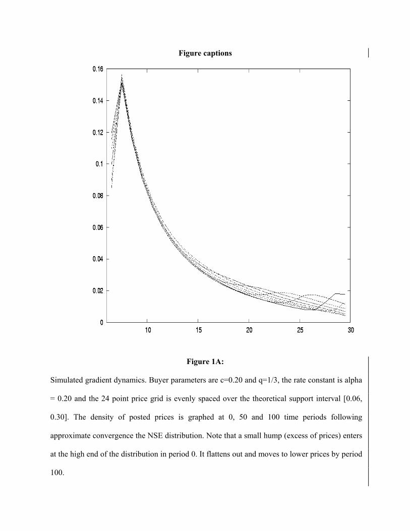
Figure captions
Figure 1A:
Simulated gradient dynamics. Buyer parameters are c=0.20 and q=1/3, the rate constant is alpha
= 0.20 and the 24 point price grid is evenly spaced over the theoretical support interval [0.06,
0.30]. The density of posted prices is graphed at 0, 50 and 100 time periods following
approximate convergence the NSE distribution. Note that a small hump (excess of prices) enters
at the high end of the distribution in period 0. It flattens out and moves to lower prices by period
100.

23
Figure 1B:
Time averages of gradient dynamics. Buyer and rate parameters are the same as in Figure 1A.
The solid lines graph densities of posted prices averaged over 50,000 time periods for evenly
spaced price grids of 10, 20, 40 and 80 points. The dashed line graphs the NSE distribution,
which assumes a price continuum.
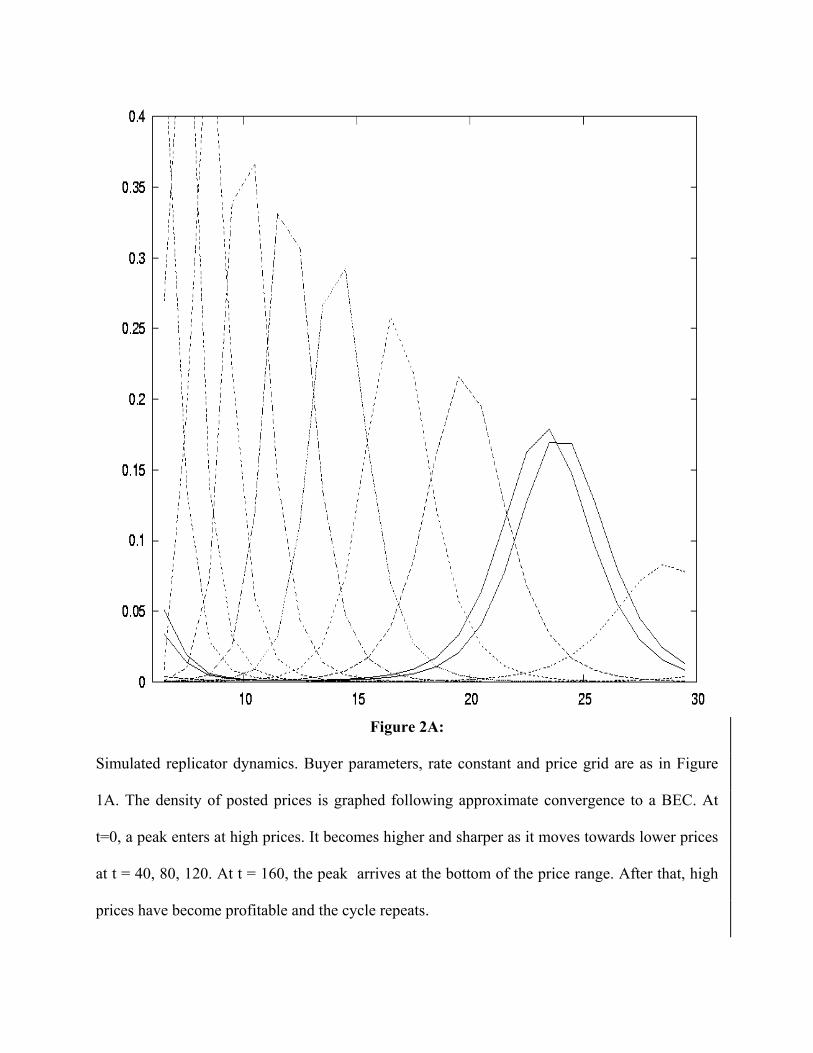
Figure 2A:
Simulated replicator dynamics. Buyer parameters, rate constant and price grid are as in Figure
1A. The density of posted prices is graphed following approximate convergence to a BEC. At
t=0, a peak enters at high prices. It becomes higher and sharper as it moves towards lower prices
at t = 40, 80, 120. At t = 160, the peak arrives at the bottom of the price range. After that, high
prices have become profitable and the cycle repeats.

25
Figure 2B:
Time averages of replicator dynamics. Parameters are as in Figure 1B. As the price grid
becomes finer, the discrete distributions (solid lines) converge to a continuous distribution that
is much less skewed (more uniform than) the NSE distribution (dashed line).
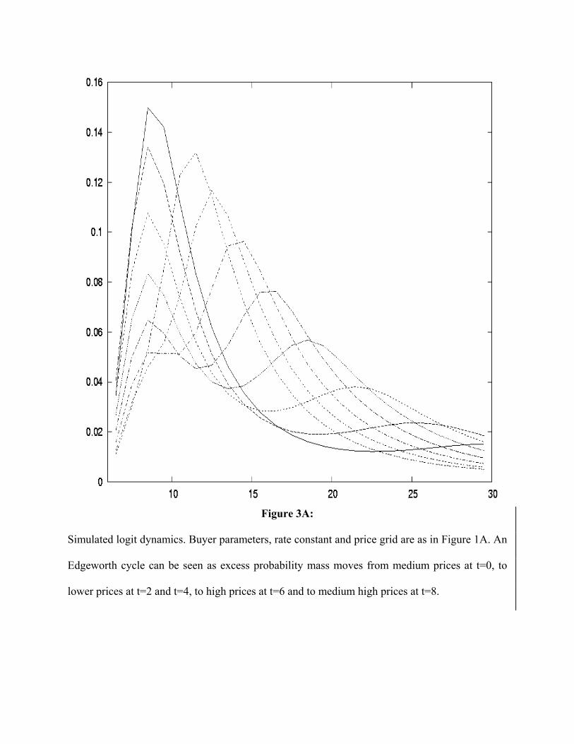
Figure 3A:
Simulated logit dynamics. Buyer parameters, rate constant and price grid are as in Figure 1A. An
Edgeworth cycle can be seen as excess probability mass moves from medium prices at t=0, to
lower prices at t=2 and t=4, to high prices at t=6 and to medium high prices at t=8.
27
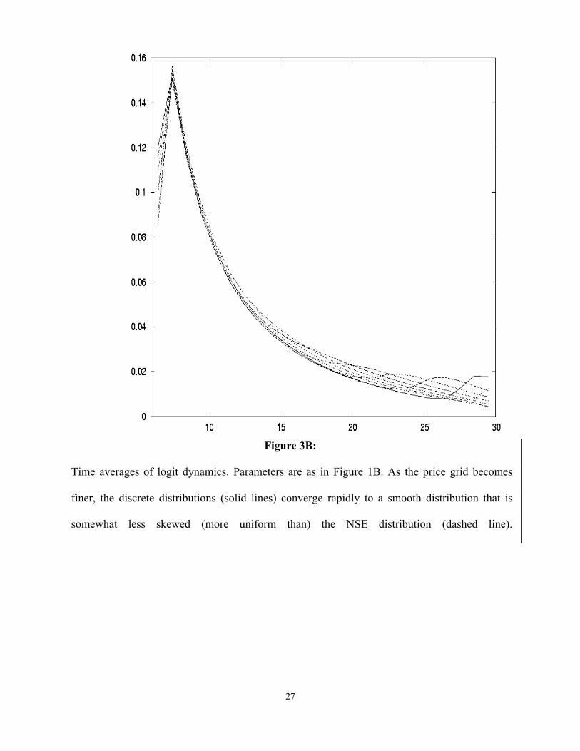
Figure 3B:
Time averages of logit dynamics. Parameters are as in Figure 1B. As the price grid becomes
finer, the discrete distributions (solid lines) converge rapidly to a smooth distribution that is
somewhat less skewed (more uniform than) the NSE distribution (dashed line).

Figure 4A:
Simulated hybrid dynamics. Buyer parameters, rate constant and price grid are as in Figure 1A.
A larger amplitude Edgeworth cycle can be seen as excess probability mass moves from medium
prices at t=0, to lower prices at t=2 and t=4, to high prices at t=6 and to medium high prices at
t=8.
29
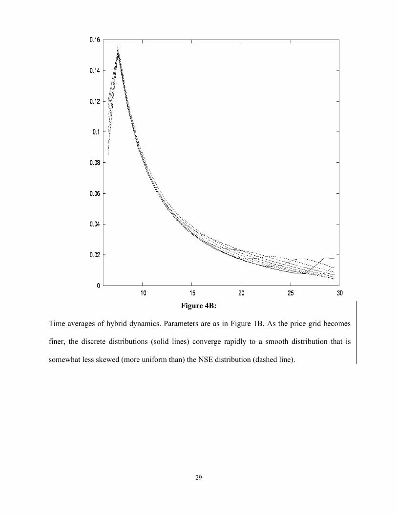
Figure 4B:
Time averages of hybrid dynamics. Parameters are as in Figure 1B. As the price grid becomes
finer, the discrete distributions (solid lines) converge rapidly to a smooth distribution that is
somewhat less skewed (more uniform than) the NSE distribution (dashed line).

Table 1: Estimated Transition Matrices for All Periods in Experienced Sessions
search cost=20 q=1/3 search cost=20 q=2/3 Observ. 1
1tQ + 1
2tQ + 1
3tQ + 1
4tQ + Observ. 1
1tQ + 1
2tQ + 1
3tQ + 1
4tQ +
82 1tQ 0.73 0.11 0.09 0.07 83 1
tQ 0.75 0.10 0.06 0.10 70 2
tQ 0.24 0.59 0.13 0.04 63 2tQ 0.22 0.62 0.08 0.08
65 3tQ 0.08 0.25 0.58 0.09 75 3
tQ 0.13 0.12 0.59 0.16 71 4
tQ 0.03 0.11 0.14 0.72 61 4tQ 0.02 0.11 0.36 0.51
search cost=60 q=1/3 search cost=60 q=2/3
Observ. 11tQ + 1
2tQ + 1
3tQ + 1
4tQ + Observ. 1
1tQ + 1
2tQ + 1
3tQ + 1
4tQ +
71 1tQ 0.63 0.18 0.07 0.11 74 1
tQ 0.66 0.16 0.09 0.08 74 2
tQ 0.24 0.55 0.14 0.07 71 2tQ 0.24 0.55 0.07 0.14
74 3tQ 0.04 0.24 0.62 0.09 71 3
tQ 0.03 0.25 0.52 0.20 69 4
tQ 0.14 0.06 0.16 0.64 72 4tQ 0.10 0.11 0.28 0.51
Table 2: Estimated Transition Matrices for All Periods in Inexperienced Sessions
search cost=20q=1/3 search cost=20 q=2/3 Observ. 1
1tQ + 1
2tQ + 1
3tQ + 1
4tQ + Observ. 1
1tQ + 1
2tQ + 1
3tQ + 1
4tQ +
44 1tQ 0.64 0.07 0.16 0.14 46 1
tQ 0.61 0.20 0.09 0.11 41 2
tQ 0.32 0.49 0.15 0.05 47 2tQ 0.28 0.40 0.15 0.17
43 3tQ 0.05 0.30 0.53 0.12 38 3
tQ 0.11 0.34 0.45 0.11 46 4
tQ 0.02 0.20 0.17 0.61 43 4tQ 0.02 0.16 0.23 0.58
search cost=60q=1/3 search cost=60 q=2/3
Observ. 11tQ + 1
2tQ + 1
3tQ + 1
4tQ + Observ. 1
1tQ + 1
2tQ + 1
3tQ + 1
4tQ +
48 1tQ 0.56 0.17 0.08 0.19 46 1
tQ 0.76 0.07 0.07 0.11 38 2
tQ 0.34 0.45 0.11 0.11 39 2tQ 0.23 0.64 0.10 0.03
42 3tQ 0.14 0.24 0.57 0.05 44 3
tQ 0.11 0.18 0.55 0.16 46 4
tQ 0.07 0.11 0.24 0.59 45 4tQ 0.02 0.04 0.27 0.67
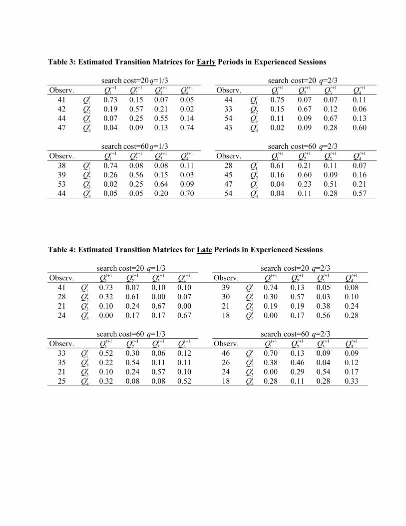
Table 3: Estimated Transition Matrices for Early Periods in Experienced Sessions
search cost=20 q=1/3 search cost=20 q=2/3 Observ. 1
1tQ + 1
2tQ + 1
3tQ + 1
4tQ + Observ. 1
1tQ + 1
2tQ + 1
3tQ + 1
4tQ +
41 1tQ 0.73 0.15 0.07 0.05 44 1
tQ 0.75 0.07 0.07 0.11 42 2
tQ 0.19 0.57 0.21 0.02 33 2tQ 0.15 0.67 0.12 0.06
44 3tQ 0.07 0.25 0.55 0.14 54 3
tQ 0.11 0.09 0.67 0.13 47 4
tQ 0.04 0.09 0.13 0.74 43 4tQ 0.02 0.09 0.28 0.60
search cost=60 q=1/3 search cost=60 q=2/3
Observ. 11tQ + 1
2tQ + 1
3tQ + 1
4tQ + Observ. 1
1tQ + 1
2tQ + 1
3tQ + 1
4tQ +
38 1tQ 0.74 0.08 0.08 0.11 28 1
tQ 0.61 0.21 0.11 0.07 39 2
tQ 0.26 0.56 0.15 0.03 45 2tQ 0.16 0.60 0.09 0.16
53 3tQ 0.02 0.25 0.64 0.09 47 3
tQ 0.04 0.23 0.51 0.21 44 4
tQ 0.05 0.05 0.20 0.70 54 4tQ 0.04 0.11 0.28 0.57
Table 4: Estimated Transition Matrices for Late Periods in Experienced Sessions
search cost=20 q=1/3 search cost=20 q=2/3 Observ. 1
1tQ + 1
2tQ + 1
3tQ + 1
4tQ + Observ. 1
1tQ + 1
2tQ + 1
3tQ + 1
4tQ +
41 1tQ 0.73 0.07 0.10 0.10 39 1
tQ 0.74 0.13 0.05 0.08 28 2
tQ 0.32 0.61 0.00 0.07 30 2tQ 0.30 0.57 0.03 0.10
21 3tQ 0.10 0.24 0.67 0.00 21 3
tQ 0.19 0.19 0.38 0.24 24 4
tQ 0.00 0.17 0.17 0.67 18 4tQ 0.00 0.17 0.56 0.28
search cost=60 q=1/3 search cost=60 q=2/3
Observ. 11tQ + 1
2tQ + 1
3tQ + 1
4tQ + Observ. 1
1tQ + 1
2tQ + 1
3tQ + 1
4tQ +
33 1tQ 0.52 0.30 0.06 0.12 46 1
tQ 0.70 0.13 0.09 0.09 35 2
tQ 0.22 0.54 0.11 0.11 26 2tQ 0.38 0.46 0.04 0.12
21 3tQ 0.10 0.24 0.57 0.10 24 3
tQ 0.00 0.29 0.54 0.17 25 4
tQ 0.32 0.08 0.08 0.52 18 4tQ 0.28 0.11 0.28 0.33

(a) (b)
(c) (d)
(e) (f) Figure 9:
Errors in c=20, q=1/3 fits. The horizontal axes show the averaging period ω for the simulated transition matrices, and the vertical axes show the (Hilbert-Schmidt) distance between the simulated matrix and the first transition matrix in Table 1. One curve is shown for each value of the parameter α: 0.05: solid line, 0.10: long dashes, 0.15: short dashes, 0.20: dots, 0.25: dash-dotted. Replicator dynamics are shown in (a), gradient in (b), logit in (c) and (d), hybrid in (e) and (f).
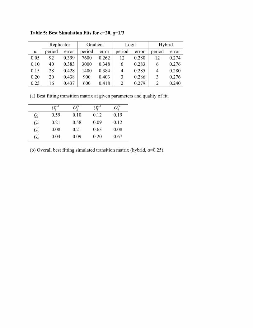
Table 5: Best Simulation Fits for c=20, q=1/3
Replicator Gradient Logit Hybrid α period error period error period error period error
0.05 92 0.399 7600 0.262 12 0.280 12 0.274 0.10 40 0.383 3000 0.348 6 0.283 6 0.276 0.15 28 0.428 1400 0.384 4 0.285 4 0.280 0.20 20 0.438 900 0.403 3 0.286 3 0.276 0.25 16 0.437 600 0.418 2 0.279 2 0.240
(a) Best fitting transition matrix at given parameters and quality of fit.
11tQ + 1
2tQ + 1
3tQ + 1
4tQ +
1tQ 0.59 0.10 0.12 0.19
2tQ 0.21 0.58 0.09 0.12
3tQ 0.08 0.21 0.63 0.08
4tQ 0.04 0.09 0.20 0.67
(b) Overall best fitting simulated transition matrix (hybrid, α=0.25).