The Dynamics of Capital Flow Episodes∗

Christian Friedrich † Pierre Guérin ‡

July 12, 2016

Abstract

In this paper, we first propose a novel methodology for identifying episodes of equityand bond flows that employs estimates from a regime-switching model, which has theadvantage of keeping context- and sample-specific assumptions to a minimum. Wethen use a time-varying structural vector-autoregressive (VAR) model to assess theimpact of U.S. stock market volatility (VIX) shocks and U.S. monetary policy shocks onaggregated measures of equity outflow and equity inflow episodes. Our results indicatethat both VIX and U.S. monetary policy shocks had substantially time-varying effectson episodes of strong capital flows over our sample period.

Keywords: capital flow episodes; Markov-switching models, global financial cycle

JEL Classification Code: F21, F32, G11

∗We would like to thank Mahvash Qureshi, Yuriy Gorodnichenko, Michael Hutchison, Nelson Mark, Jean-Marie Dufour, Oleksiy Kryvtsov, Garima Vasishtha, Gurnain Pasricha, Louphou Coulibaly, participants ofthe 2016 Applied Time Series Econometrics Workshop held at the Federal Reserve Bank of St. Louis, the14th INFINITI Conference on International Finance in Dublin, the 50th Annual Conference of the CanadianEconomic Association in Ottawa and seminar participants at the Bank of Canada for helpful comments. Theviews expressed in this paper are those of the authors. No responsibility for them should be attributed tothe Bank of Canada. An earlier version of this paper is available as Bank of Canada Staff Working Paper2016-9.†Bank of Canada, International Economic Analysis Department, 234 Laurier Avenue West, Ottawa, ON,

K1A 0G9, Canada; e-mail: cfriedrich@bankofcanada.ca‡Bank of Canada, International Economic Analysis Department, 234 Laurier Avenue West, Ottawa, ON,

K1A 0G9, Canada; e-mail: pguerin@bankofcanada.ca

1 IntroductionFollowing the triad of events comprising the global financial crisis, unconventional monetarypolicies and negative interest rates in many advanced economies, the assessment of globalcapital flow dynamics has forcefully re-entered the research agendas of policy-makers andacademics. In particular, these recent experiences have renewed the interest in investigatingand understanding the determinants and consequences of international capital flows.

Building on the seminal work of Forbes and Warnock (2012) and Ghosh et al. (2014),who classify episodes of strong capital flows in quarterly and annual data, respectively, wecontribute to this research agenda in two ways.1 First, using equity and bond fund flow dataat a weekly frequency, we employ a novel methodology for identifying episodes of strong cap-ital flows in high-frequency data that is based on estimates from a regime-switching model.A key advantage of regime-switching models is that they allow us to determine the under-lying regimes endogenously, without the need for context- and sample-specific assumptions.Moreover, using high-frequency data is important, since it allows us to obtain a timely andprecise classification of sharp movements in capital flows, which would be difficult to obtainwith Balance of Payments (BoP) data due to their lower release frequencies and publicationlags. Second, we then use a structural vector-autoregressive (VAR) model with time-varyingparameters to study the dynamic interactions between aggregated measures of equity flowepisodes and global drivers of capital flows, such as U.S. stock market volatility shocks andU.S. monetary policy shocks, over time.

Our first contribution relates to a growing literature that examines consequences andimplications of international capital flows. In particular, it concentrates on the impact ofcapital flows on destination countries, mostly emerging markets. Examples of such impactsare credit booms and currency mismatches on the financial side and appreciating currenciesand inflationary developments from a macroeconomic perspective. To investigate these issues,the literature makes increasing use of episode classifications to separate extended periods ofstrong capital flows from regular fluctuations.2

In the context of international capital flows, an episode classification is particularly helpfulfor two reasons. First, since capital flows are volatile (e.g., see Bluedorn et al. (2013)),the aggregation of individual capital flow observations into episodes can provide a clearerpattern of the direction and the magnitude of flows. Second, the literature has shown thatthe macroeconomic effects of capital flows can differ according to the level of capital flows

1Earlier studies that have empirically identified episodes of strong capital flows are Calvo et al. (2004) for“sudden stop” episodes as well as Reinhart and Reinhart (2009) and Cardarelli et al. (2010) for “surges.”

2Examples of studies that have recently worked with episode classifications are Caballero (2014), Magudet al. (2014), Benigno et al. (2015), and Eichengreen and Gupta (2016).

1

(e.g., see Abiad et al. (2009)). Thus, some of the macroeconomic or financial effects of capitalflows can only be observed when the level of flows reaches a certain magnitude.

The corresponding classification of capital flow episodes has mainly been popularized byForbes and Warnock (2012) and Ghosh et al. (2014). Forbes and Warnock (2012) divideepisodes of strong capital flows into “surges” (inflows of capital from foreigners), “stops”(outflows of capital from foreigners), “retrenchments” (inflows of capital from residents) and“capital flights” (outflows of capital from residents). Based on a threshold approach thatidentifies deviations from a long-term average as periods of strong capital flows, the authorsapply these categorizations to gross capital flows from the BoP in a sample of 58 emergingand developed economies at quarterly frequencies between 1980 and 2009. Ghosh et al.(2014) instead focus on surges of net capital flows. The authors use a related, but differentlydefined, identification methodology than in Forbes and Warnock (2012) and apply theirepisode definitions to annual BoP data in a sample of 56 emerging-market economies between1980 and 2011.

Complementing quarterly and annual classifications of capital flow episodes with a classi-fication for high-frequency data is desirable for at least two reasons. First, from an academicview point, it is important to better understand the transmission of shocks across the globalfinancial system, such as the impact of U.S. monetary policy shocks and U.S. stock marketvolatility shocks on other countries. Amplified by high levels of financial integration andthe widespread use of the U.S. dollar, these shocks can be transmitted rapidly into domesticfinancial systems with potentially adverse implications for financial stability. Second, from amore practical view point, it is often of first order importance for central banks and variousother policy institutions to monitor international capital flow dynamics in a timely manner.Since BoP data are released at low frequencies and with substantial time lags, the use ofweekly capital flow data provides timely information for monitoring emerging patterns morethoroughly and gives policy-makers additional time to respond.

Based on data that record equity and bond fund flows into up to 80 different countries3

at weekly frequency over the period 2000 to 2014, we identify episode types that are mostclosely related to the definition of surges and stops by Forbes and Warnock (2012) andpartially to the definition of net surges by Ghosh et al. (2014). Following the application ofour methodology, we show that the differences in estimated in- and outflow regimes withina country correlate negatively with the quality of its institutions and the level of financialdevelopment as well as positively with the country’s share of foreign currency liabilities. Wealso document the main features of equity and bond flow episodes, such as their frequencyof appearance and their average length for both advanced and emerging-market economies.

3There are 65 countries in our equity sample and 66 countries in our bond sample. The notion of 80different countries emerges since several countries appear in only one of the two samples.

2

Our second contribution, the subsequent analysis of aggregated capital flow dynamics,relates to a stream of literature that assesses the determinants of international capital flows.Dating back at least to Calvo et al. (1993), who introduced the distinction between interna-tional “push” and domestic “pull” factors, a rich body of literature developed and culminatedin a wealth of studies analyzing capital flow dynamics during and after the global financialcrisis.4 Our analysis relates in particular to recent work by Rey (2013), who argues that assetprices and capital flows closely follow the dynamics of U.S. monetary policy and U.S. stockmarket volatility. Rey suggests that this so called “global financial cycle” reduces the tradi-tional trilemma – the impossibility of having independent monetary policy, an open capitalaccount and a fixed exchange rate at the same time – to a dilemma by leaving policy-makersonly the choice between independent monetary policy and an open capital account, even inthe presence of a freely floating exchange rate. Hence, the effects that U.S. macroeconomicand financial shocks have on international capital flows are of high interest to policy-makersand academics.

The results of our structural VAR analysis indicate that both U.S. stock market volatility,measured by the VIX,5 and U.S. monetary policy had substantially time-varying effects onepisodes of strong capital flows over our sample period. The impact of a VIX shock has beenstronger in times of crises but has almost consistently led to more equity outflow episodesand fewer equity inflow episodes in each period. The impact of a U.S. monetary policyshock, however, has changed sign over our sample period in that, in the wake of the financialcrisis, such a shock has led to more equity outflow episodes and fewer equity inflow episodescompared with the pre-crisis period. On the one hand, our results support the earlier findingsby Rey (2013) that U.S. macroeconomic and financial shocks affect the economic and financialcycles of other countries substantially. On the other hand, our results show that the impactof these shocks on the rest of the world differs substantially over time – making it potentiallyeven more difficult for policy-makers elsewhere to design an appropriate policy response.

Our paper is organized into four sections and proceeds as follows. After this introduction,Section 2 presents our methodology for identifying episodes of strong capital flows, henceforthsimply referred to as “episodes,”6 in high-frequency data. In particular, this section containsa description of the empirical methodology and a discussion of our episode-classification re-

4The most prevalent methods in the literature are factor models (e.g., Forster et al. (2014), Puy (2016),and, with a focus on the global financial crisis, Fratzscher (2012)); and panel data models (e.g., Ahmed andZlate (2014); Bruno and Shin (2015a), and, with a focus on the global financial crisis, Milesi-Ferretti andTille (2011)). Also, the cyclical properties of capital flows have been analyzed frequently (e.g., Contessi et al.(2013), Broner et al. (2013), and Bussière et al. (2016)).

5VIX refers to the CBOE index of implied volatility on S&P500 options.6Periods with strong capital inflows are referred to as “inflow episodes” and periods with strong capital

outflows are referred to as “outflow episodes.”

3

sults. Section 3 then presents the results of a structural VAR analysis that assesses theimpact of VIX shocks and U.S. monetary policy shocks on aggregated measures of equityinflow and outflow episodes across our sample countries. Finally, Section 4 concludes.

2 Classification of Capital Flow EpisodesThis section proposes a methodology that is well suited for identifying capital flow episodes

in high-frequency data and novel in the context of capital flows. We first highlight the mo-tivation for adapting a new methodology in the context of high-frequency data, characterizethe nature of our data and describe our econometric approach. We then present the outcomeof the estimation process and discuss the results of our empirical analysis.

2.1 Episode Classification Methodology

2.1.1 Motivation

While the most common methodology to identify capital flow episodes in the existingliterature is based on a threshold approach, which assigns periods with above-threshold valuesthe label of an “episode,” there is no agreement on how to design the underlying threshold.Forbes and Warnock (2012) and Ghosh et al. (2014), for example, use two largely differentthreshold definitions to identify episodes of “surges” in BoP data.

Forbes and Warnock (2012), on the one hand, compute rolling means and standard de-viations of year-on-year changes in quarterly gross capital flows over the last five years. Theauthors then define a surge episode as fulfilling two conditions: (i) capital flow dynamics areeligible for an episode classification as long as the year-on-year changes in capital flows aregreater than one standard deviation above the rolling mean; and (ii) to be eventually countedas an episode, there must be an increase of year-on-year changes in capital flows of more thantwo standard deviations above the rolling mean during at least one quarter of the episode.Ghosh et al. (2014), on the other hand, work with data at annual frequency and define a surgeepisode based on the following two conditions: (i) an observation is eligible to be classifiedas a surge episode if it lies in the top 30th percentile of the country’s own distribution of netcapital flows (as a percentage of GDP); and (ii) to be eventually counted as an episode, theobservation also has to be in the top 30th percentile of the entire (cross-country) sample’sdistribution of net capital flows (as a percentage of GDP).

However, even if there was a common approach in the literature, threshold values couldrequire additional adjustments depending on the characteristics of the dataset, such as datafrequency (e.g., annual vs. higher-frequency), country type (e.g., advanced economies vs.

4

emerging markets), time period (e.g., inclusion of the 1980s, the global financial crisis, etc.)asset class (e.g., foreign direct investment vs. portfolio flows) and capital flow definition (e.g.,gross vs. net flows). While episode classifications based on threshold approaches for low-frequency data have served well in the past and have been generally in line with anecdotalevidence, it is challenging to convincingly select the appropriate threshold for high-frequencydata in the absence of a “true” benchmark for capital flow episodes. In particular, exogenouslyimposed thresholds based on moments of the capital flow distribution for annual or quarterlydata may not be appropriate for high-frequency data, which is characterized by a higherdegree of volatility.

We therefore propose a novel methodology for identifying capital flow episodes in high-frequency data based on estimates from a set of country-specific regime-switching models thatallow us to determine the underlying regimes endogenously, without the need to make explic-itly context- and sample-specific assumptions. This approach is also particularly suitable tomonitor capital flow movements in real-time, which is of prime importance for policy-makers.7

2.1.2 Data

We use weekly data from the Emerging Portfolio Fund Research (EPFR) database, whichrecords international equity and bond fund flows at high frequencies. The EPFR data havefeatured prominently in the literature, such as in Jotikasthira et al. (2012) and in Fratzscher(2012), who recently used major components of the data that we are employing. In addition,Fratzscher states that the EPFR’s fund flow data “[...] is the most comprehensive one ofinternational capital flows, in particular at higher frequencies and in terms of its geographiccoverage at the fund level.”

There are two main differences between equity and bond fund flows from the EPFRdatabase and conventional BoP data. The first difference refers to the coverage of assetclasses. BoP data, on the one hand, records all foreign direct investment flows, portfolioequity and debt investment flows as well as other investment flows (which are mostly bankflows) of a country. The EPFR data, on the other hand, cover only portfolio equity and debtinvestments and thus do not represent the universe of capital flows.8 The second differencerelates to the coverage of financial system participants. While the BoP records cross-bordercapital flows by all participants of the financial system, regardless of their location, the EPFR

7In addition, most of the definitions of capital flow episodes in the literature lead to a binary indicatorthat provides limited information on how distant the actual data are from the threshold. In contrast, aprobabilistic approach, such as the one introduced below, could better reflect the uncertainty surroundingthe estimation of capital flow episodes, and how likely a country is to enter or exit such episodes, whichconstitutes important information for policy-makers and financial market participants.

8One important implication of this fact is that capital inflows and outflows across all sample countries donot necessarily sum to zero in our analysis.

5

data are limited to international investments that are intermediated by equity and bond fundsand thus comprise only a subset of financial system participants as well as only those capitalmovements that originate abroad (i.e., from non-residents). However, since the segment ofequity and bond fund flows is an important part of total flows and financial transactions bynon-residents have traditionally been highly relevant, in particular for emerging markets, themore timely available EPFR database has become a key data source for policy institutions.

Further, Pant and Miao (2012) show for emerging-market economies that there is a strongcorrespondence between the U.S.-dollar values of EPFR and BoP data. Since our measureof capital flows is defined as the percentage change in outstanding investments, we presentadditional evidence in this paper that the alternative measurement of capital flows does notaffect the comparability of data across the two sources. In particular, we compare the quarter-on-quarter growth rates of weekly EPFR data and quarterly BoP data for equity inflows intoBrazil.9 Figure 1 indicates that the two growth rates follow each other closely and showsthat their correlation coefficient amounts to 0.54. Hence, these observations suggest thatthe weekly EPFR data and the quarterly BoP data experience largely similar capital flowdynamics.

The EPFR data that we use are aggregated to the destination country level and arecharacterized by the “country flows” concept, which is defined as the product of capital inflowsinto investment funds (i.e., the “fund flows” dimension) and the respective country allocationof these investment funds (i.e., the “country allocation” dimension).10 We therefore obtain acountry-time-specific value of net capital inflows for each country. The data are expressed asa percentage change in outstanding investments (i.e., the total estimated allocation of moneyin absolute dollar terms) at the start of the period (i.e., the previous week).11

9For the EPFR data, which record equity inflows as the percentage change in outstanding equity invest-ments at the start of a week, we conduct the following modifications. First, we apply all weekly percentagechanges in equity inflows into Brazil to an index that takes on the value of 100 at the beginning of oursample. Second, we use this cumulated series of week-on-week growth rates to derive the correspondingquarter-on-quarter growth rates. For the BoP data, we start from a measure that captures the quarterlychange in Brazil’s net foreign equity liabilities in U.S. dollars. First, to normalize this series by the equivalentof the outstanding investments, we take the ratio of the U.S.-dollar figure to quarterly GDP. Second, wecumulate the series and derive the corresponding quarter-on-quarter growth rate. While the overlappingperiod between both data sources is 2001 to 2011, we start the comparison in 2002 to reduce the impact ofthe initial growth rates.

10Consider the following example: To calculate the country flows to Country X, the fund weightings forCountry X are multiplied by each fund group’s net fund flows for the period. The resulting country flow isthen an estimate of how much new investor money will be put to work in Country X.

11In the EPFR database, this definition is denoted as “Country Flow/US$%”. We also do not restrictinvestment funds to be from a specific source country and thus use investment funds from “all domiciles” inour sample.

6

We treat the data for equity and bond flows separately as they come with varying countrycoverage and sample start dates. The final sample for equity flows contains data from 65advanced and emerging-market countries, and the start date ranges from the last week ofOctober 2000 to the last week of July 2006, depending on data availability (precise detailson the criteria we used to select the underlying series are presented in Appendix A).12 Thefinal dataset of bond flows contains 66 countries and the start date extends from the firstweek of January 2004 to the first week of January 2006. The end date of both the estimationsamples is the last week of December 2014. Finally, to reduce the impact of outliers in theempirical analysis, we winsorize the capital flow data of each country at the top 1 per centand the bottom 1 per cent of the capital flow distribution.

Our data choice determines also the types of episodes that we can identify. As pointedout in the introduction, Forbes and Warnock (2012) and Ghosh et al. (2014) are the twomost closely related studies that identify capital flow episodes. Using data from the EPFRdatabase with the above discussed characteristics, we can identify two types of episodes:“inflow episodes” – corresponding to the surges definition from Forbes and Warnock (2012) –and “outflow episodes” – corresponding to their definition of stops.13 While there is a certaincorrespondence between our measure of inflow episodes and the measure of net flow surgesfrom Ghosh et al. (2014), the results of our analysis will be more closely related to those ofForbes and Warnock (2012), since the definition of net flow surges in Ghosh et al. (2014)contains capital movements by residents, for which we do not have data.

2.1.3 The Regime-Switching Model

Regime-switching models have been used in economics and finance since the seminalwork of Hamilton (1989). In particular, they have been widely applied in the context ofbusiness cycle analysis (see, for example, Chauvet (1998)) and empirical macroeconomicsto study, for example, the effects of monetary policy across different regimes (see Sims andZha (2006)). Likewise, there is a vast body of literature on regime changes in finance (see,e.g., the literature review in Ang and Timmermann (2012)). The underlying idea of Markov-switching models is to estimate discrete changes from a continuous variable. Hence, whenstudying capital flows, regime-switching models allow us to estimate discrete shifts in thedata from the (continuous) capital flows series.

12The emerging-market sample contains a few countries that are generally considered to be low-incomecountries rather than emerging markets. However, in order to keep the analysis tractable, we refer to thegroup of emerging-market and low-income countries as “emerging markets” in the remainder of the paper.

13Investments (disinvestments) in investment funds by residents of a large country can take on traces ofcapital flights (retrenchments), when the associated fund is predominantly funded from the home country.However, given that we do not restrict the selection of investment funds along the geographical dimension,the investments carried out by residents of a single country should be sufficiently small.

7

Following Baele et al. (2014), who estimate a three-regime Markov-switching model usingequity and bond returns to estimate flight-to-safety episodes, we fit a three-regime Markov-switching model to the EPFR equity and bond flow series. The first regime with a negativeintercept (i.e., µ1 < 0) is associated with strong outflows, the third regime with a positiveintercept (i.e., µ3 > 0) is associated with strong inflows, and the second regime is a “normal”regime, where capital flows exhibit neither strong increases nor strong decreases (i.e., µ1 <

µ2 < µ3). A key advantage of using data at a weekly frequency is that it allows us to bettertrack fluctuations in capital flows.14 In detail, the baseline univariate model we estimate is

yi,t = µi(St) + εi,t(St), (1)

where εi,t|St ∼ N(0,σ2i ), and yi,t is the portfolio data associated with either equity or bond

flows for country i at time t.15 We estimate all regime-switching models with quasi-maximumlikelihood, using the expectation-maximization algorithm (see Hamilton (1990)).16

2.2 Episode Classification Results

2.2.1 Estimation Results from the Regime-Switching Model

Table 1 presents the results of the country-specific regime-switching models that wereestimated separately for equity and bond flows. The table shows the average parameterestimates of all sample countries as well as the average of the parameter estimates calculatedfrom advanced and emerging markets only (see Appendix B for a definition of these countrygroupings). For illustrative purposes, we also report individual estimation results for theUnited States and Brazil – an advanced country and an emerging market from our dataset.

The results indicate that the first regime is systematically associated with (large) negativeoutflows (i.e., µ1 < 0), and the third regime with large positive inflows (i.e., µ3 > 0 andµ3 > µ2). Finally, the second or “normal” regime is characterized by neither strong inflowsnor strong outflows (i.e., µ1 < µ2 < µ3).17 Moreover, the differences in the intercepts’

14Note that EPFR data are also available at a daily frequency. However, following Fratzscher (2012), werefrain from using such data because it is unlikely that fund managers make portfolio decisions at such highfrequency.

15Note that we also model changes in the variance of the innovation, since we obtained a better fit withsuch a specification. The innovation variance in the second regime is systematically lower than the innovationvariance in the other two regimes.

16The regime-switching models are estimated with the GAUSS 9.0 software without imposing constraintson the model parameters, except for the transition probabilities to ensure irreducibility of the Markov chain.

17We also implemented the Carrasco et al. (2014) test for regime-switching parameters in the mean andvariance of equation (1). In all cases, we found overwhelming evidence in favor of regime-switching parameters.Detailed results are available on request.

8

estimates, defined as µ3 − µ1, in both equity and bond flows are lower for the group ofadvanced economies than for the group of emerging markets in our sample.

Figure 2 explores this finding further and provides correlation evidence between the dif-ferences in intercepts across regimes (left axes), i.e., µ3 − µ1, and potential explanatoryvariables (bottom axes). The six variables are the gross domestic product (GDP) per capitain purchasing-power-parity (PPP) units (to represent the income difference between bothcountry groups), the real GDP growth rate in percent, a measure of institutional quality,private credit as a percentage of GDP, stock market capitalization as a percentage of GDPand the share of liabilities in foreign currency.18 In the first five cases, we observe a negativecorrelation, suggesting that a higher per capita income, more real GDP growth, a higherquality of institutions and more financial development are associated with a lower differencein the intercepts of the two extreme regimes for a country. In addition, a higher share offoreign currency liabilities is associated with a larger difference in regime intercepts. Hence,in line with the previous literature on boom and bust cycles in emerging markets, thesecorrelations suggest that countries, which are characterized by poor macroeconomic/growthperformance, weak institutions (e.g., Klein (2005)), a low level of financial development (e.g.,Caballero and Krishnamurthy (2001)) and a high share of foreign currency liabilities (e.g.,Eichengreen et al. (2003)), will experience more distinct inflow and outflow regimes; that is,more abrupt changes in capital flows.

Turning next to the transition probabilities, we find that regimes in advanced economiesare more persistent than in emerging-market economies. This is the case because the tran-sition probabilities of staying in each regime (p11, p22, and p33), are systematically higher inthe first compared to the second country group. When focusing on the unconditional prob-abilities of being in a certain regime, it turns out that overall the second regime is the mostprevalent one, since the unconditional probability of being in the second regime, (P (St = 2)),is the highest compared with those of being in any of the other regimes in almost all cases.

Finally, the individual estimation results for the United States and Brazil confirm theevidence obtained from the aggregated results. In particular, we find for both equity andbond flows that the differences in regime intercepts are smaller for the United States thanfor Brazil, that regimes are more persistent in the United States than in Brazil and thatboth countries will spend most of the time in the second regime. However, relative to theUnited States, Brazil is more likely to spend time in the two extreme regimes (because theunconditional probabilities of the first and the third regime are higher for Brazil).

18To reduce the impact of capital flows on these variables, we rely on the 1999 values of all six variables.

9

2.2.2 Episode Classification and Discussion of Findings

Based on Table 2, this section presents and discusses the classification of different types ofepisodes and their appearance across different country groupings. We obtain a separate setof episodes for equity outflows, equity inflows, bond outflows and bond inflows and presentthese results aggregated across all sample countries, across all advanced countries and acrossall emerging markets of our sample.19 The column “Avg. Probability” in Panel A presentsthe average probability of being in a different regime than the normal regime. To movefrom here to a discrete outcome variable that indicates the presence of a distinct patternof capital flows, we define two additional conditions that, when fulfilled, characterize an“episode.”20 Both conditions are based on information contained in the smoothed regimeprobabilities. The first condition is that the probability of being in a regime other than thenormal one is greater than 50 percent. The second condition is that this is the case for atleast four consecutive weeks. The column “Avg. Share in Episode” presents the result of thecorresponding episode classification by indicating the average time of the sample period thatthe three country groupings spend in each type of episode. Moreover, the column labelled“Frequency” indicates the frequency with which each type of episode appears over the sampleperiod and the column “Avg. Length” contains information on its associated average length.Based on Panel A of Table 2, we derive five facts from the episode classification exercise.

First, even though the average probability obtained from the regime-switching model isby definition higher than the average share of inflow and outflow episodes, the similarity ofboth series suggests that periods of strong capital flows generally extend beyond four weeks.

Second, the average country in the sample spends between 21.1 and 26.8 percent of thetime in each type of episode. While, the average time that advanced and emerging marketsspend in each type of bond flow episode is very similar (i.e., 19.5 and 21.8 for bond outflowsfrom advanced countries and emerging markets, respectively; 26.2 and 27.1 for bond inflowsinto both country groupings, respectively), the average time that advanced countries spend inboth types of equity flow episodes is significantly larger than the time that emerging marketsspend in such episodes (i.e., 33.2 and 22.1 for equity outflows from advanced countries andemerging markets; 29.4 and 19.5 for equity inflows into both regions, respectively).

Third, we observe that the average country in the sample faces equity flow episodes morefrequently than bond flow episodes (i.e., 12.8 equity outflow and 9.9 equity inflow episodescompared with 7.3 bond outflow and 8.0 bond inflow episodes). While the distribution offrequencies between advanced and emerging-market economies is fairly similar in three out

19The disaggregated country-specific results are available on request.20These assumptions are only required to convert the probabilities of being in a given regime into discrete

measures of episodes as they are commonly used in the literature. Depending on the application, one couldwork with these probabilities directly and there would be no need for any additional assumptions.

10

of the four cases, equity outflow episodes have a significantly higher frequency in emergingmarkets (14.7 cases for the average emerging country) than in advanced countries (9.3 casesfor the average advanced country).

Fourth, we see that for the average country in the sample, the length of outflow episodes(i.e., 17.4 weeks for equity outflow episodes and 16.8 weeks for bond outflow episodes) isshorter than the length of inflow episodes (i.e., 20.0 weeks for equity inflow episodes and19.0 weeks for bond inflow episodes). We also observe that advanced countries (between21.2 weeks in the case of bond outflow episodes and 30.3 weeks in the case of equity outflowepisodes) experience a significantly higher persistence of episodes than emerging markets(between 10.4 weeks for equity outflow episodes and 17.0 weeks for bond inflow episodes).

Finally, in Panel B of Table 2, we examine the contemporaneous correlation coefficientof episodes across asset classes for the entire sample as well as for advanced countries andfor emerging markets separately.21 A strong positive correlation between both capital classescould be an indication that investors do not substantially differentiate between asset classeswithin countries (e.g., because of the presence of country-specific risks or a lack of informationabout a country). A negative number, on the other hand, could point to a higher differenti-ation because of fewer country-specific risks or a better availability of information. Startingwith the correlation between equity outflows and bond outflows, the number for the overallsample amounts to 0.36 and indicates that both asset classes behave in a fairly synchronizedway. Splitting up the number into a separate one for the two country groupings shows thatinvestors differentiate more often between asset classes in advanced countries (where thecorrelation amounts to 0.27) than in emerging markets (where the correlation amounts to0.42). The correlation between equity inflows and bond inflows for the average country in theoverall sample is somewhat lower and amounts to 0.17, with, again, a higher correlation co-efficient for the average emerging market (0.26) than for the average advanced country (0.05).

3 Equity Flow Episodes and the Global Financial CycleIn this section, we study the dynamic interactions between the share of countries in equity

flow episodes and a set of global factors, such as U.S. stock market volatility and the U.S.monetary policy stance, using vector-autoregression (VAR) models along the lines of Brunoand Shin (2015b). Thematically, our analysis relates closely to the literature on the globalfinancial cycle, proposed by Rey (2013), who argues that the VIX is the main driver ofinternational capital flows and asset prices and that U.S. monetary policy shocks in turn arestrong drivers of the VIX. We conduct our analysis using first a linear VAR, followed by a

21The disaggregated country-specific results are available on request.

11

time-varying parameter VAR that allows us to model the changing impact of the two shockson our measures of capital flow episodes over time.

3.1 Empirical Methodology

3.1.1 Data

Our VAR models build on the empirical methodology in Bruno and Shin (2015b). Weadapt their VAR specification for the international dimension to our research question byreplacing their measure of international bank flows with our measure of countries in capitalflow episodes. As in Bruno and Shin (2015b), we further include the U.S. real federal fundsrate, to measure the U.S. monetary policy stance, and the VIX, to capture U.S. stock mar-ket volatility. We deviate slightly from their specification (i) by replacing their measure ofbanking sector leverage with a measure of the U.S. business cycle since our research questiondeals with market-based instead of bank-based financial intermediation and (ii) by abstract-ing from the computation and inclusion of a real effective exchange rate as its value-added ina cross-country sample is very limited. Next, we describe the variables included in our VARmodels in detail:

Capital Flow Episodes: We use the share of countries in an equity outflow episode andthe share of countries in an equity inflow episode as two separate measures of capital flowepisodes across countries.22 In doing so, we rely on a measure that comprises all countries inour sample as well as on two other measures that focus on the country groupings of emergingmarkets and advanced economies, respectively. We concentrate our analysis on equity flowdata, since bond flow data are available only over a shorter sample period. Figures 3 and4 present the share of countries in an equity outflow and an equity inflow episode (for theentire sample and for both country groupings separately). The peaks of the outflow sharemeasures are located in the aftermath of the dot-com bubble and during the global financialcrisis. The peaks of the inflow share measures are clustered in the four years prior to theglobal financial crisis and appear sporadically during the post-crisis period as well.

U.S. Stock Market Volatility: We use the CBOE index of implied volatility on S&P500options (VIX) in the VAR system, since it is a commonly used measure of global financialmarket volatility (see, e.g., Rey (2013)). The VIX is an attractive measure to proxy theglobal financial cycle in that it directly captures not only financial market volatility, but alsouncertainty to the extent that it is related to financial markets fluctuations.

22Note that we use the share of countries in a given regime directly in the VAR model for consistency inthe analysis throughout the paper, but impulse responses based on a log scale for the share of countries in agiven regime yield qualitatively similar results.

12

U.S. Monetary Policy Stance: A standard choice for evaluating the effects of monetarypolicy is to use the effective federal funds rate (see, e.g., Christiano et al. (1999) or Bernankeet al. (2005)). However, as the federal funds rate reached the zero lower bound in December2008 and the Federal Reserve started large-scale asset purchases, the short-term interest rateno longer conveyed comprehensive information about the stance of U.S. monetary policy. Asa result, our measure of monetary policy is the effective federal funds rate until December2008, complemented by the Wu and Xia (2015) shadow federal funds rate for the periodextending from January 2009 to December 2014.23 As in Bruno and Shin (2015b), we use thereal federal funds rate; that is, we subtract the annual change in the CPI from the nominalshort-term rate. Figure 5 represents this measure of monetary policy, i.e., the real federalfunds rate until December 2008, and the estimated real shadow interest rate from January2009.

U.S. Business Cycle Fluctuations: Finally, we use U.S. industrial production as a mea-sure of business cycle fluctuations (taken as 100 times the change in the log index), since itis a widely used measure of U.S. monthly economic activity.

While Bruno and Shin (2015b) do not include pull factors, such as the state of the businesscycle and the monetary policy stance in countries other than the U.S., in their specification,it should be noted that the relevance of pull factors as determinants of international capitalflows has been demonstrated in the past. We therefore check the correlation between ourmeasure of the U.S. business cycle and the (real) U.S. monetary policy stance with theirrespective counterparts calculated from all other countries in our sample. Since we obtainhighly positive correlations of 0.79 in case of the median (0.79 in case of the mean) for thebusiness cycle and of 0.78 (0.58) for the real policy interest rate, we follow Bruno and Shin(2015b) again and abstract from pull factors in our analysis as well.24

23In detail, Wu and Xia (2015) derive a shadow interest rate from a term-structure model. Based on thisshadow interest rate, they find that monetary policy affects the U.S. macroeconomic environment in a similarfashion in the post- and pre-Great Recession periods, suggesting that using the Wu and Xia (2015) shadowfederal funds rate from January 2009 onwards is appropriate to study the effects of monetary policy in asample that includes zero lower bound episodes.

24It should further be noted that the identification of episodes has been conducted separately for eachcountry so that the intercepts of the Markov-switching models are country-specific. This implicitly controlsfor all country-specific factors that are time-invariant.

13

3.1.2 VAR Methodology

Linear VAR ModelWe first conduct our analysis with a linear VAR model. The reduced-form version of the

model is a K-dimensional VAR(p) model

Yt = ν + A1Yt−1 + ...+ ApYt−p + Ut, (2)

where Yt is a (K×1) vector of observable time series, ν is a constant term, the Ajs (j = 1, ..., p)are (K ×K) coefficient matrices and Ut is a zero-mean error term. The structural shocks εt

we are interested in are obtained from the reduced-form residuals by a linear transformation,εt = B−1Ut, where B is such that εt has an identity covariance matrix; that is, εt ∼ (0, IK)and the reduced-form residual covariance matrix is decomposed as E(UtU

′t ) = ΣU = BB′.

The model is identified using a recursive structure, i.e., choosing the B matrix by a Choleskidecomposition so as to achieve identification. Our baseline specification includes the fourfollowing variables in this order: industrial production, the real interest rate, the VIX, anda measure of capital flow episodes.

In doing so, we assume a recursive structure in the system, ordering the variables fromslow- to fast-moving. As a result, the measure of capital flow episodes is placed last inthe VAR, which assumes that the capital flow variable reacts contemporaneously to all othervariables in the system (i.e., business cycle measure, monetary policy measure, and the VIX).The VIX is placed third in the system so that it reacts contemporaneously to the businesscycle and monetary policy variables. The monetary policy measure is placed second in theVAR, which implies that it reacts only contemporaneously to the business cycle variable.Finally, our measure of business cycle activity is placed first in the VAR system, whichassumes that the business cycle variable is predetermined in that it is affected only with alag by the other variables in the system.

The model is estimated with standard least squares, and the lag length of the VAR isselected according to the Akaike information criterion. The sample size extends from April2001 to December 2014. Note also that the analysis is done at a monthly, and not weekly, fre-quency for two main reasons. First, some of the variables in the system are not available at aweekly frequency (e.g., U.S. industrial production or the Wu and Xia (2015) shadow interestrate). Second, conducting the analysis at a monthly frequency permits a more straightfor-ward comparison with the existing literature, since this type of structural VAR analysis istypically done at a monthly or quarterly frequency.

Time-Varying Parameter VAR ModelWe then extend our analysis of equity flow episodes to a time-varying parameter (TVP)

VAR. One caveat of the linear VAR model represented in Equation (2) is that impulse

14

responses derived from this model are constant over time. However, there are a numberof reasons to think that this assumption may potentially be too restrictive. For example,following the unconventional monetary policy measures employed in a number of advancedeconomies, it could well be that capital flows react differently to monetary policy shocksafter the global financial crisis than during the pre-crisis period. Likewise, in the wake of theglobal financial crisis, the changing landscape of the financial sector could affect global riskaversion and, hence, change the reaction of capital flows to volatility shocks. As a result, wealso estimate a TVP-VAR model, which can be seen as a general approximation to the linearmodel described in Equation (2). This permits us to evaluate the degree of time variationin the impulse responses. Following Primiceri (2005), we estimate a TVP-VAR model withstochastic volatility using Bayesian methods. This model can be written as follows

Yt = νt + A1,tYt−1 + ...+ Ap,tYt−p + Vt, (3)

where Vt ∼ N(0,Σt) are the reduced-form shocks with a (K × K) heteroskedastic VARcovariance matrix, Σt. We estimate a model with two autoregressive lags, but the results arerobust to the inclusion of additional autoregressive lags. We define αt = [νt, A1,t, ..., Ap,t]′ asthe vector of parameters in the model (stacked by rows), which evolve according to a driftlessrandom walk process

αt = αt−1 + et, et ∼ iidN(0, Q). (4)

The variance-covariance matrix Q is assumed to be diagonal, and the innovations et areassumed to be uncorrelated with the VAR innovations Vt. The innovations Vt are normallydistributed, and their variances are time-varying

Vt ∼ N(0,Σt), Σt = B−1t Ht(B−1

t )′. (5)

The matrix Bt (that summarizes the contemporaneous relationships between the K variablesin the system) is a lower triangular matrix with ones on its diagonal; that is, we assume thesame identification scheme as in the linear case. The dynamics of the non-zero and non-oneelements of Bt are governed by the following dynamics

Bt = Bt−1 + lt, var(lt) = D. (6)

The matrix Ht is a diagonal matrix with elements hi,t, following a geometric random walk

ln(hi,t) = ln(hi,t−1) + ηi,t, ηi,t ∼ iidN(0, σ2i ), (7)

for i = {1, 2, 3, 4}. Additional details on the model and the estimation method are reportedin Appendix C.

15

3.2 Global Financial Cycle Results

3.2.1 Results from the Linear VAR

We start by presenting the results from the linear VAR. Figure 6 reports the impulse-response functions for the share of countries in an equity outflow episode following a VIXshock and a U.S. monetary policy shock.25

First, we assess the impact of the VIX shock (i.e., a 10-point increase in the VIX26) onthe outflow share measure, which is displayed in the first panel of the top row in Figure 6.When considering an unexpected increase in the VIX, we observe a sharp increase in theshare of countries in an outflow episode upon impact (about 15 percent). This increase inthe share measure is statistically significant on impact, since the associated bootstrapped 90percent confidence bands are above zero. This is in line with economic theory: an increasein the VIX indicates a higher level of stock market volatility and proxies for uncertaintyin financial markets. In such an environment, investors are more likely to withdraw theirequity fund investments and move to safer asset classes, such as government bonds, instead.Hence, equity outflow episodes appear more often across countries and thus the outflow sharemeasure increases. Further, the confidence bands show that the reaction of the outflow sharemeasure to a VIX shock is relatively short-lived, with an insignificant response after twomonths. However, short-lived reactions are not unusual in the context of high-frequencyfinancial data, where the inflow and outflow cycles are considerably shorter than in lower-frequency data.

Second, we assess the impact of a U.S. monetary policy shock (i.e., a 100-basis-pointincrease in the real federal funds rate) on the outflow share measure, which is shown inthe first panel of the bottom row of Figure 6. For the linear VAR, it turns out that theU.S. monetary policy shock has essentially no significant impact on the share of countriesin an outflow episode. However, the expected sign of the effect is not clear a priori. Onthe one hand, a higher real interest rate could proxy for higher investment returns,27 andthus, following a increase in the interest rate, we would observe a reduction in the share of

25For completeness, we also report the impulse responses of the other variables in the system to these twoshocks. The results are as follows. The response of the VIX to its own shock documents the persistence ofthe shock, the response of the U.S. real interest rate is slightly positive, but largely insignificant, and theeffect of the VIX on U.S. industrial production is negative. The response of the VIX to the U.S. monetarypolicy shock is negative but largely insignificant, the response of the U.S. real interest rate documents thepersistence of the shock, and the response of U.S. industrial production to the U.S. monetary policy shock isnegative (and again largely insignificant).

26This is of similar magnitude as a one-standard-deviation change of the VIX in our sample, which amountsto 8.6 points.

27In fact, in such a case, the presence of a spread over the U.S. interest rate would most likely increaseinterest rates in all other countries more than proportionally.

16

countries in an outflow episode.28 On the other hand, a higher real interest rate can be asign of tighter financial conditions and thus an indication of increased risks. This, in turn,could lead to an increase in the share of countries in an outflow episode. Since it is possiblethat, in light of our above discussed finding, different interpretations have played a role atdifferent points in time, we return to this observation in Section 3.2.2.29 This finding is,however, consistent with the linear VAR results in Bruno and Shin (2015b), who do not finda statistically significant initial response of the international bank flow measure to a shockin the real fed funds rate either. It also lines up with the results of Dahlhaus and Vasishtha(2014), who identify a “monetary policy normalization shock” in a linear VAR system thatincludes a factor extracted from capital flows going to emerging-market economies. In detail,they identify a monetary policy normalization shock as a shock that increases both the yieldspread of U.S. long-term bonds and monetary policy expectations, while leaving the policyrate unchanged. Their results suggest that a monetary policy normalization shock in theUnited States has a relatively small economic impact on emerging-market portfolio flows.

Next, we conduct the same exercises for equity inflow episodes. Figure 7 reports theresponses of the share of countries in an equity inflow episode to a VIX shock (first panel,top row) and to a U.S. monetary policy shock (first panel, bottom row).30 First, as expected,a surprise increase in the VIX leads to a decline in the share of countries in an inflowepisode. Hence, an increase in uncertainty leads to a sharp reduction of equity fund flowsthat materializes in our analysis in the form of a lower share of countries experiencing suchepisodes. However, the largest effect appears on impact again and fades out very quickly.Note also that, in absolute value, the reaction on impact is somewhat smaller comparedwith Figure 6, suggesting some evidence for non-linear effects. In other words, U.S. stockmarket volatility shocks seem, on average, to affect outflow episodes relatively more thaninflow episodes. Second, the bottom row reports the responses of the same set of variablesto a U.S. monetary policy shock. The main result is that, in the linear VAR, an increase

28Relatedly, and in particular during the period when the U.S. short-term interest rate was at the zerolower bound, an increase in the (nominal) interest rate can be seen as an improvement in the Fed’s view ofthe U.S. economy and thus a sign of economic recovery and higher growth. Such an interpretation wouldalso support the evidence of a decrease in the share of countries in an outflow regime following an increasein interest rates.

29In Section 3.2.2, we will use a time-varying parameter VAR to assess whether the effects of U.S. monetarypolicy on capital flow dynamics may have changed over recent years.

30We again report the impulse-response functions of the other variables for completeness. The response ofthe VIX to its own shock shows the persistence of the shock; that the response of the U.S. real interest rate tothe VIX shock is positive, but largely insignificant; and that U.S. industrial production responds negatively.The response of the VIX to the U.S. monetary policy shock is negative, the response of the U.S. real interestrate to its own shock indicates the shock persistence again, and the impact on U.S. industrial production isslightly negative but insignificant again.

17

in the real interest rate leads to a significant increase in the share of countries in an inflowepisode. Following the explanation above, this finding appears to assign more weight to aninterpretation of the real interest rate as a measure of returns than as a measure of risks.

So far, we have conducted our analysis for share measures that comprise all countries in thesample. However, since the previous literature has found substantial differences in capitalflow dynamics between advanced economies and emerging markets, we also compare theimpulse-response functions for both country groupings separately. In doing so, we estimatethe VAR model represented by Equation (2) using the share of countries in an outflow andan inflow episode, respectively, calculated only from advanced economies, and only fromemerging markets. Figure 8 reports the difference between the impulse responses obtainedfrom emerging markets and advanced economies to a VIX shock and a U.S. monetary policyshock.31

A VIX shock, that had an overall increasing effect on the share of countries in an outflowepisode, has an even stronger impact on emerging markets, which is shown by the positive andsignificant impact in the difference-impulse-response function in the top left panel of Figure8. This finding is suggested by economic theory and previous analyses in the literature(e.g., Gourio et al. (2014)). Since investments in emerging markets are generally riskier, anincrease in uncertainty will affect emerging-market investments more than proportionally.Moving then to the U.S. monetary policy shock, which in the full sample had no significantimpact on the share of countries in outflow episodes, the difference-impulse-response functionin the bottom left panel does not show a difference between emerging markets and advancedcountries on impact either.

We also assess the differential impact on inflow episodes across country groupings. Start-ing with the response to a VIX shock, which in the full sample had a reducing effect on theshare of countries in an inflow episode but faded out very quickly, we observe a strong differ-ence between both groups. The positive response of the difference-impulse-response functionin the top right panel of Figure 8 suggests that the impact of the VIX shock on inflow episodesis more positive/less negative for emerging markets than for advanced countries. Finally, weexamine the impact of a monetary policy shock that, overall, increased the share of countriesin an inflow regime. Based on the insignificant difference-impulse-response function in thebottom right panel, however, we observe that there is no significant difference between thetwo country groupings.

31We compute the difference of the two impulse-response functions (IRF) as follows: IRF (Difference) =IRF (Emerging Markets) – IRF (Advanced Countries).

18

3.2.2 Results from the Time-Varying Parameter VAR

We now provide results from the time-varying parameter VAR to investigate the degree oftime variation in the impulse responses. Figure 9 shows the time-varying impulse responsesto a VIX shock and to a U.S. monetary policy shock using the share of countries in an outflowepisode as a measure of capital flow dynamics.

Starting with the response to a VIX shock in Panel (a), we observe that the impact ofa surprise increase in the VIX on the share of countries in an outflow episode is positivethroughout the sample period but varies significantly over time. A shock in the VIX hasa stronger impact during the period of the financial crisis and at the very recent end ofthe sample. This suggests evidence in favour of a non-linearity, such as the effect of a VIXshock seems greater in turbulent times. However, with an increase in the VIX resulting inan increase in the share of outflows, throughout the sample, the results from the linear VARare generally confirmed.32

Next, Panel (b) depicts the response to the U.S. monetary policy shock. Interestingly, weobserve a highly time-varying pattern in the case of our share measure for equity outflowsthat explains the, on average, insignificant response of this variable to a U.S. monetarypolicy shock in the linear VAR. While the impact of a U.S. monetary policy shock on theshare measure was negative from the beginning of our sample until around 2011, the shareof countries in an equity outflow episode increases in response to a U.S. monetary policyshock after this date.33 Potential explanations for this finding have already been presentedabove. A negative relationship between the unexpected increase in the U.S. real interest rateand the share of countries in an outflow episode in the early part of the sample, possiblyrepresents a return-based interpretation of the real interest rate; that is, investors invest incountries where returns, here proxied by the real interest rate, are higher. In contrast, themore recently observed positive relationship between an unexpected increase in the U.S. realinterest rate and the share of countries in an outflow episode, favours an interpretation basedon risks. That is, following a tightening of U.S. monetary policy in the aftermath of thefinancial crisis,34 investors might have found it less attractive to invest in risky investmentsabroad.35 A possible explanation for the observed change in the response of the outflow

32To conserve space, we do not report the time-varying responses of the other variables in the system. Theresponses are as follows. The U.S. real interest rate responds to the VIX shock in a similar way throughoutthe sample with an unexpected increase in the VIX having a positive effect on this variable. The impact ofthe VIX on U.S. industrial production is negative throughout.

33Note that 68 percent posterior credible sets exclude a zero response of the share of countries in an equityoutflow episode after 2011.

34It should be noted that the tightening of U.S. monetary policy refers to an increase in the shadow interestrate.

35The other variables react to a U.S. monetary policy shock as follows. An increase in the U.S. real interestrate leads to a reduction in the VIX. However, the impulse-response function from the time-varying parameter

19

episode share measure to the U.S. monetary policy shock over our sample period might beassociated with a re-pricing of risks that occurred in the aftermath of the global financialcrisis.

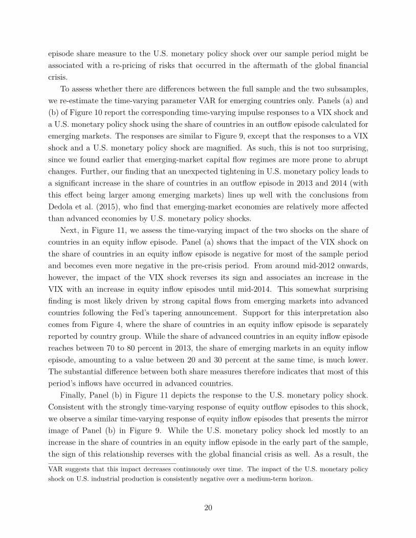
To assess whether there are differences between the full sample and the two subsamples,we re-estimate the time-varying parameter VAR for emerging countries only. Panels (a) and(b) of Figure 10 report the corresponding time-varying impulse responses to a VIX shock anda U.S. monetary policy shock using the share of countries in an outflow episode calculated foremerging markets. The responses are similar to Figure 9, except that the responses to a VIXshock and a U.S. monetary policy shock are magnified. As such, this is not too surprising,since we found earlier that emerging-market capital flow regimes are more prone to abruptchanges. Further, our finding that an unexpected tightening in U.S. monetary policy leads toa significant increase in the share of countries in an outflow episode in 2013 and 2014 (withthis effect being larger among emerging markets) lines up well with the conclusions fromDedola et al. (2015), who find that emerging-market economies are relatively more affectedthan advanced economies by U.S. monetary policy shocks.

Next, in Figure 11, we assess the time-varying impact of the two shocks on the share ofcountries in an equity inflow episode. Panel (a) shows that the impact of the VIX shock onthe share of countries in an equity inflow episode is negative for most of the sample periodand becomes even more negative in the pre-crisis period. From around mid-2012 onwards,however, the impact of the VIX shock reverses its sign and associates an increase in theVIX with an increase in equity inflow episodes until mid-2014. This somewhat surprisingfinding is most likely driven by strong capital flows from emerging markets into advancedcountries following the Fed’s tapering announcement. Support for this interpretation alsocomes from Figure 4, where the share of countries in an equity inflow episode is separatelyreported by country group. While the share of advanced countries in an equity inflow episodereaches between 70 to 80 percent in 2013, the share of emerging markets in an equity inflowepisode, amounting to a value between 20 and 30 percent at the same time, is much lower.The substantial difference between both share measures therefore indicates that most of thisperiod’s inflows have occurred in advanced countries.

Finally, Panel (b) in Figure 11 depicts the response to the U.S. monetary policy shock.Consistent with the strongly time-varying response of equity outflow episodes to this shock,we observe a similar time-varying response of equity inflow episodes that presents the mirrorimage of Panel (b) in Figure 9. While the U.S. monetary policy shock led mostly to anincrease in the share of countries in an equity inflow episode in the early part of the sample,the sign of this relationship reverses with the global financial crisis as well. As a result, the

VAR suggests that this impact decreases continuously over time. The impact of the U.S. monetary policyshock on U.S. industrial production is consistently negative over a medium-term horizon.

20

U.S. monetary policy shock is associated with a reduction of equity inflow episodes acrosscountries, particularly since the beginning of the post-crisis period in 2010.

Overall, our empirical analysis suggests that unexpected changes in both the VIX and inU.S. monetary policy have had time-varying effects on the dynamics of equity flow episodesover our sample period. On the one hand, these findings support the earlier observationsthat U.S. macroeconomic and financial shocks substantially affect the economic and financialcycles of other countries as suggested by Rey (2013). On the other hand, these findingsdemonstrate that the impact of both shocks on the rest of the world differs substantiallyover time – making it potentially even more difficult for policy-makers abroad to design anappropriate policy response. However, it should be mentioned that our VAR approach doesnot explicitly disentangle the roles of push and pull factors as drivers of capital flows (e.g.,such as in Fratzscher (2012)) nor does it directly address the economic and financial effectsof unconventional monetary policies (e.g., such as in Forbes et al. (2016)). Both researchquestions are beyond the scope of this paper and are left for future research.

4 ConclusionThis paper has identified episodes of strong capital flows in weekly fund flow data and assessedtheir dynamics for a large set of advanced and emerging economies. It has contributed tothe literature along two dimensions.

First, we have proposed a novel methodology for identifying episodes of strong capitalflows that is suitable for high-frequency data. In particular, we have estimated regime-switching models on data of equity and bond fund flows into up to 80 different countriesat weekly frequency over the period 2000 to 2014. A key advantage of this approach isto endogenously determine capital flow regimes without the need for context- and sample-specific assumptions that might be hard to derive in a convincing way when data are sampledat a high frequency. Operating at high-frequency is important since it allows us to obtain aprecise and timely characterization of capital flow episodes. Based on this analysis, we haveshown that differences in estimated inflow and outflow regimes within countries correlatepositively with the quality of institutions and the level of financial development as well asnegatively with a country’s share of foreign currency liabilities. We have also documentedthe main features of equity and bond flow episodes, such as the time a typical country spendsin different episodes types as well as their frequency of appearance and their average length.

Second, we then have used linear and time-varying structural VARs to assess the impact ofU.S. stock market volatility shocks and U.S. monetary policy shocks on aggregated measuresof equity outflow and equity inflow episodes. Our results indicate that both the VIX andthe U.S. monetary policy shock had substantially time-varying effects on episodes of strong

21

capital flows over our sample period. The impact of a VIX shock has been stronger in times ofcrises but has almost consistently led to more equity outflow episodes and fewer equity inflowepisodes in each period. The impact of a U.S. monetary policy shock, however, has changedsign over our sample period in that, in the wake of the financial crisis, such shocks have ledto more equity outflow episodes and fewer equity inflow episodes compared with the pre-crisis period. Overall, finding evidence in favor of a time-varying response of capital flows toshocks originating in the U.S. is an important input into the current debate on internationalspillover effects of U.S. monetary policy decisions and highlights additional challenges thatpolicy-makers abroad might face when designing their intended policy responses.

ReferencesAbiad, A., Leigh, D., and Mody, A. (2009). Financial integration, capital mobility, andincome convergence. Economic Policy, 24:241–305.

Ahmed, S. and Zlate, A. (2014). Capital flows to emerging market economies: A brave newworld? Journal of International Money and Finance, 48(PB):221–248.

Ang, A. and Timmermann, A. (2012). Regime Changes and Financial Markets. AnnualReview of Financial Economics, 4(1):313–337.

Baele, L., Bekaert, G., Inghelbrecht, K., and Wei, M. (2014). Flights to Safety. Finance andEconomics Discussion Series 2014-46, Board of Governors of the Federal Reserve System(U.S.).

Benati, L. (2014). Economic Policy Uncertainty and the Great Recession. Mimeo.

Benigno, G., Converse, N., and Fornaro, L. (2015). Large Capital Inflows, Sectoral Allocation,and Economic Performance. Journal of International Money and Finance, 55:60–87.

Bernanke, B., Boivin, J., and Eliasz, P. S. (2005). Measuring the Effects of Monetary Policy:A Factor-augmented Vector Autoregressive (FAVAR) Approach. The Quarterly Journal ofEconomics, 120(1):387–422.

Bluedorn, J. C., Duttagupta, R., Guajardo, J., and Topalova, P. (2013). Capital Flows areFickle: Anytime, Anywhere. IMF Working Papers 13/183, International Monetary Fund.

22

Broner, F., Didier, T., Erce, A., and Schmukler, S. L. (2013). Gross capital flows: Dynamicsand crises. Journal of Monetary Economics, 60(1):113–133.

Bruno, V. and Shin, H. S. (2015a). Capital flows and the risk-taking channel of monetarypolicy. Journal of Monetary Economics, 71(C):119–132.

Bruno, V. and Shin, H. S. (2015b). Cross-Border Banking and Global Liquidity. Review ofEconomic Studies, 82(2):535–564.

Bussière, M., Schmidt, J., and Valla, N. (2016). International Financial Flows in the NewNormal: Key Patterns (and Why We Should Care). CEPII Policy Brief 2016-10, CEPIIresearch center.

Caballero, J. (2014). Do Surges in International Capital Inflows Influence the Likelihood ofBanking Crises? Economic Journal, forthcoming.

Caballero, R. J. and Krishnamurthy, A. (2001). International and domestic collateral con-straints in a model of emerging market crises. Journal of Monetary Economics, 48(3):513–548.

Calvo, G. A., Izquierdo, A., and Mejía, L.-F. (2004). On the empirics of Sudden Stops: therelevance of balance-sheet effects. Proceedings, Federal Reserve Bank of San Francisco,(Jun).

Calvo, G. A., Leiderman, L., and Reinhart, C. M. (1993). Capital Inflows and Real ExchangeRate Appreciation in Latin America: The Role of External Factors. IMF Staff Papers 40(1).

Cardarelli, R., Elekdag, S., and Kose, M. A. (2010). Capital inflows: Macroeconomic impli-cations and policy responses. Economic Systems, 34(4):333 – 356.

Carrasco, M., Hu, L., and Ploberger, W. (2014). Optimal Test for Markov Switching Param-eters. Econometrica, 82(2):765–784.

Chauvet, M. (1998). An Econometric Characterization of Business Cycle Dynamics withFactor Structure and Regime Switching. International Economic Review, 39(4):969–96.

Christiano, L. J., Eichenbaum, M., and Evans, C. L. (1999). Monetary policy shocks: Whathave we learned and to what end? In Taylor, J. B. and Woodford, M., editors, Handbookof Macroeconomics, volume 1 of Handbook of Macroeconomics, chapter 2, pages 65–148.

Cogley, T. and Sargent, T. J. (2005). Drift and Volatilities: Monetary Policies and Outcomesin the Post WWII U.S. Review of Economic Dynamics, 8(2):262–302.

23

Contessi, S., De Pace, P., and Francis, J. L. (2013). The cyclical properties of disaggregatedcapital flows. Journal of International Money and Finance, 32(C):528–555.

Dahlhaus, T. and Vasishtha, G. (2014). The Impact of U.S. Monetary Policy Normalizationon Capital Flows to Emerging-Market Economies. Bank of Canada Working Paper, No.2014-53.

Dedola, L., Rivolta, G., and Stracca, L. (2015). If the Fed sneezes, who gets a cold? Mimeo.

Eichengreen, B., Hausmann, R., and Panizza, U. (2003). Currency Mismatches, Debt In-tolerance and Original Sin: Why They Are Not the Same and Why it Matters. NBERWorking Papers 10036, National Bureau of Economic Research, Inc.

Eichengreen, B. J. and Gupta, P. D. (2016). Managing sudden stops. Policy ResearchWorking Paper Series 7639, The World Bank.

Forbes, K., Reinhardt, D., and Wieladek, T. (2016). The spillovers, interactions, and(un)intended consequences of monetary and regulatory policies. Bank of England Dis-cussion Paper No. 44, Bank of England.

Forbes, K. J. and Warnock, F. E. (2012). Capital flow waves: Surges, stops, flight, andretrenchment. Journal of International Economics, 88(2):235–251.

Forster, M., Jorra, M., and Tillmann, P. (2014). The dynamics of international capital flows:Results from a dynamic hierarchical factor model. Journal of International Money andFinance, 48(PA):101–124.

Fratzscher, M. (2012). Capital flows, push versus pull factors and the global financial crisis.Journal of International Economics, 88(2):341–356.

Ghosh, A. R., Qureshi, M. S., Kim, J. I., and Zalduendo, J. (2014). Surges. Journal ofInternational Economics, 92(2):266–285.

Gourio, F., Siemer, M., and Verdelhan, A. (2014). Uncertainty and International CapitalFlows. Mimeo.

Hamilton, J. D. (1989). A New Approach to the Economic Analysis of Nonstationary TimeSeries and the Business Cycle. Econometrica, 57(2):357–84.

Hamilton, J. D. (1990). Analysis of time series subject to changes in regime. Journal ofEconometrics, 45(1-2):39–70.

24

Jotikasthira, C., Lundblad, C., and Ramadorai, T. (2012). Asset Fire Sales and Purchasesand the International Transmission of Funding Shocks. Journal of Finance, 67(6):2015–2050.

Klein, M. W. (2005). Capital Account Liberalization, Institutional Quality and EconomicGrowth: Theory and Evidence. NBER Working Papers 11112, National Bureau of Eco-nomic Research, Inc.

Lane, P. R. and Shambaugh, J. C. (2010). Financial Exchange Rates and InternationalCurrency Exposures. American Economic Review, 100(1):518–40.

Magud, N. E., Reinhart, C. M., and Vesperoni, E. R. (2014). Capital Inflows, Exchange RateFlexibility and Credit Booms. Review of Development Economics, 18(3):415–430.

Milesi-Ferretti, G.-M. and Tille, C. (2011). The great retrenchment: international capitalflows during the global financial crisis. Economic Policy, 26(66):285–342.

Pant, M. and Miao, Y. (2012). Coincident Indicators of Capital Flows. IMF Working Papers12/55, International Monetary Fund.

Primiceri, G. E. (2005). Time Varying Structural Vector Autoregressions and MonetaryPolicy. Review of Economic Studies, 72(3):821–852.

Puy, D. (2016). Mutual funds flows and the geography of contagion. Journal of InternationalMoney and Finance, 60(C):73–93.

Reinhart, C. and Reinhart, V. (2009). Capital Flow Bonanzas: An Encompassing View ofthe Past and Present. NBER International Seminar on Macroeconomics 2008, pages 9–62.

Rey, H. (2013). Dilemma not trilemma: the global cycle and monetary policy independence.Proceedings, Economic Policy Symposium in Jackson Hole.

Sims, C. A. and Zha, T. (2006). Were There Regime Switches in U.S. Monetary Policy?American Economic Review, 96(1):54–81.

Wu, J. C. and Xia, F. D. (2015). Measuring the Macroeconomic Impact of Monetary Policyat the Zero Lower Bound. Journal of Money, Credit, and Banking, forthcoming.

25

Appendices

A Dataset ConstructionThis appendix provides a summary of the steps required to construct our sample of

equity and bond capital flows based on the EPFR database. In general, data availability isdetermined by the EPFR data and differs between equity and bond flows.

A.1 Equity Flows

• We download weekly data on capital flows, aggregated to the destination country level,from equity funds, based in all domiciles, between the last week of October 2000 andthe last week of December 2014:

– For 108 countries/regional aggregates, there is at least one observation in the data.

– For 47 countries/regional aggregates, the data are entirely complete over the period(i.e., 741 observations).

– For 61 countries/regional aggregates, there is at least one observation missing (thenumber of missing observations ranges between 2 and 739).

• In order to have a continuous time series of data (which is required by our empiricalapproach), we drop all countries that have a missing value between the first week ofJanuary 2007 and the last week of December 2014 (8 years):

– This leaves 71 countries/regional aggregates in the sample.

• From this set of countries/regional aggregates, we eliminate (i) all regional aggregates,(ii) all observations before the first missing observation in each country, and (iii) SaudiArabia (where equity flow dynamics during our sample period contain strong outliers).

– Hence, the final sample of equity flows contains 65 countries with start datesranging from the last week of October 2000 to the last week of July 2006.

A.2 Bond Flows

• We download weekly data on capital flows, aggregated to the destination country level,from bond funds, based in all domiciles, between the first week of January 2004 andthe last week of December 2014:

26

– For 122 countries/regional aggregates, there is at least one observation in the data.

– For 43 countries/regional aggregates, the data are entirely complete over the period(i.e., 574 observations).

– For 79 countries/regional aggregates, there is at least one observation missing (thenumber of missing observations ranges between 9 and 570).

• In order to have a continuous time series of data (which is required by our empiricalapproach), we drop all countries/regional aggregates that have a missing value betweenthe first week of January 2007 and the last week of December 2014 (8 years):

– This leaves 71 countries/regional aggregates in the sample.

• From this set of countries/regional aggregates, we eliminate (i) all regional aggregates,and (ii) all observations before the first missing observation in each country.

– Hence, the final sample of bond flows contains 66 countries with start dates rangingfrom the first week of January 2004 to the first week of January 2006.

B Definition of Country GroupingsThe samples for equity and bond flows are not identical since, in some countries, data areonly available for a single asset class (E = equity sample only; B = bond sample only).

The full sample includes all countries that are available from the following two lists.

The advanced-country sample contains Australia, Austria, Belgium, Canada, Denmark,Finland, France, Germany, Greece, Ireland, Israel, Italy, Japan, Korea, Netherlands, NewZealandE, Norway, PortugalE, Spain, Sweden, Switzerland, United Kingdom, and the UnitedStates.

The emerging-market sample includes36 Argentina, Bosnia and HerzegovinaB, Brazil,BulgariaE, Chile, China, Colombia, Costa RicaB, Croatia, CyprusE, Czech Republic, Do-minican RepublicB, EcuadorB, Egypt, El SalvadorB, EstoniaE, GhanaB, GuatemalaB, Hong

36As pointed out in the main text, the emerging-market sample contains a few countries that are generallyconsidered to be low-income countries rather than emerging markets. However, in order to keep the analysistractable, we refer to the group of emerging markets and low-income countries as “emerging markets.”

27

Kong, Hungary, India, Indonesia, IraqB, Ivory CoastB, Kazakhstan, LebanonB, LithuaniaE,Malaysia, MauritiusE, Mexico, MoroccoE, Nigeria, OmanE, Pakistan, Panama, Peru, Philip-pines, Poland, QatarB, Romania, Russia, SerbiaB, Singapore, SloveniaE, South Africa, SriLankaE, TaiwanE, Thailand, Trinidad and TobagoB, Tunisia, Turkey, Ukraine, UruguayB,VenezuelaB, Vietnam, ZambiaE, and ZimbabweE.

C The Markov-Chain Monte Carlo ProcedureThis appendix provides details on the Markov-chain Monte Carlo (MCMC) procedure.

We follow Benati (2014) for the presentation of the prior distributions and the simulation ofthe posterior distribution.

C.1 Prior Distributions

The model has two sets of time-varying coefficients, the αts and the bij,ts, as well as astochastic volatility model for the diagonal elements of Ht (i.e., the hi,ts).

To calibrate the priors on α0, b0, and h0, we use the estimates of a linear VAR modelestimated over the period extending from April 2001 to March 2005. (The actual estimationsample runs from April 2003 to December 2014; that is, we discard only half of the obser-vations in the initial estimation sample so as not to eliminate too many observations.) Theprior for α0 is set as follows

α0 ∼ N [α̂OLS, 4V̂ (α̂OLS]. (C-1)

We define the matrix C as the matrix resulting from the Cholesky factorization of thevariance-covariance matrix of the residuals from the linear VAR (i.e., CC ′ = Σ̂OLS), andset the prior for h0 as

ln(h0) ∼ N(ln(µ0), 10× In), (C-2)

where µ0 is a vector collecting the logarithms of the squared elements on the diagonal of C,n is the number of variables in the system and In is the identity matrix with dimension n.Each column of C is then divided by the corresponding element on the diagonal of C, so thatwe obtain a matrix denoted as C̃ and the prior for b0 is set as

b0 ∼ N(b0, V (b0)), (C-3)

where b0 is a vector collecting all the non-zero and non-one elements from C̃−1 (e.g., forthe four-variable VAR, b0 = [b0,21, b0,31, b0,32, b0,41, b0,42, b0,43]′), and its covariance matrix,

28

V (b0) is assumed to be diagonal with elements equal to ten times the absolute value ofthe corresponding elements in b0.

Following the literature, we assume that all innovations in the model are distributed asmultivariate normal distribution with zero mean and the following diagonal structure

V = var

εt

et

lt

ηt

=

In 0 0 00 Q 0 00 0 D 00 0 0 W

, (C-4)

where ηi,t ∼ N(0,W ).The matrix Q – which governs the amount of time variation in the VAR parameters αt –

is assumed to follow an inverted Wishart distribution

Q ∼ IW (Q−10 , T0), (C-5)

with prior degrees of freedom T0 and scale matrix T0Q̄. T0 is set to the length of β plus one.Q̄ is calibrated as Q̄ = γ × Σ̂OLS, setting γ to 3.5

9 × 10−4.37

The three blocks of D are assumed to follow inverted Wishart distribution; that is,

Di ∼ IW (T, L′

itLit +Di,0), (C-6)

where T represents the degrees of freedom and the scale parameter is L′itLit +Di,0. The prior

scale matrix for D1,0 is set to 10−3, the prior scale matrix for D2,0 is set to 10−3× I2 and theprior scale matrix for D3,0 is set to 10−3 × I3.

For the variances of the stochastic volatility innovations, we assume that the σis followan inverse gamma distribution for the elements of W ; that is,

σ2i ∼ IG((0.01/3)2

2 ,12). (C-7)

C.2 Posterior Distribution Simulations

The Carter and Kohn algorithm is combined with the Metropolis-Hastings (MH) algo-rithm to sample sequentially the different sets of parameters conditional on the other blocksof parameters since sampling directly from the joint posterior distribution is not straightfor-ward.

37Based on quarterly data, Cogley and Sargent (2005) set γ = 3.5 × 10−4, which is modified as γ =( 3.5

9 )× 10−4 = ( 3.512×10−2

3 )2, since we deal with monthly data.

29

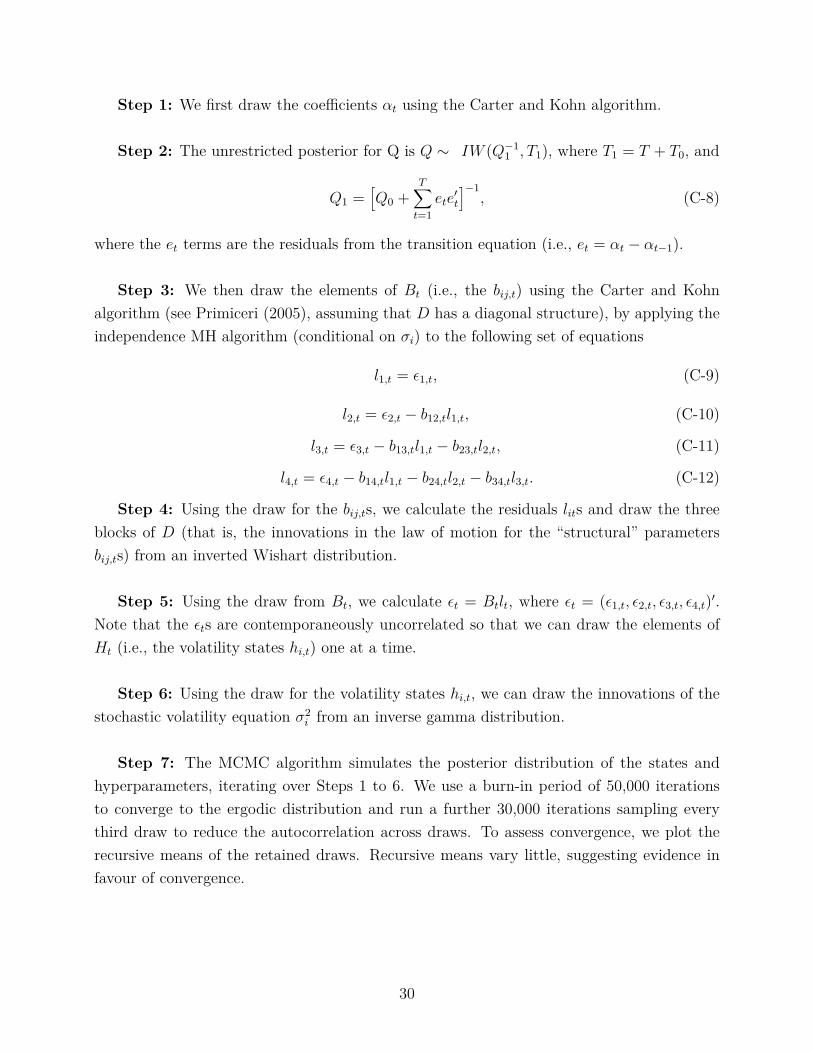
Step 1: We first draw the coefficients αt using the Carter and Kohn algorithm.

Step 2: The unrestricted posterior for Q is Q ∼ IW (Q−11 , T1), where T1 = T + T0, and

Q1 =[Q0 +

T∑t=1

ete′t

]−1, (C-8)

where the et terms are the residuals from the transition equation (i.e., et = αt − αt−1).

Step 3: We then draw the elements of Bt (i.e., the bij,t) using the Carter and Kohnalgorithm (see Primiceri (2005), assuming that D has a diagonal structure), by applying theindependence MH algorithm (conditional on σi) to the following set of equations

l1,t = ε1,t, (C-9)

l2,t = ε2,t − b12,tl1,t, (C-10)

l3,t = ε3,t − b13,tl1,t − b23,tl2,t, (C-11)

l4,t = ε4,t − b14,tl1,t − b24,tl2,t − b34,tl3,t. (C-12)

Step 4: Using the draw for the bij,ts, we calculate the residuals lits and draw the threeblocks of D (that is, the innovations in the law of motion for the “structural” parametersbij,ts) from an inverted Wishart distribution.

Step 5: Using the draw from Bt, we calculate εt = Btlt, where εt = (ε1,t, ε2,t, ε3,t, ε4,t)′.Note that the εts are contemporaneously uncorrelated so that we can draw the elements ofHt (i.e., the volatility states hi,t) one at a time.

Step 6: Using the draw for the volatility states hi,t, we can draw the innovations of thestochastic volatility equation σ2

i from an inverse gamma distribution.

Step 7: The MCMC algorithm simulates the posterior distribution of the states andhyperparameters, iterating over Steps 1 to 6. We use a burn-in period of 50,000 iterationsto converge to the ergodic distribution and run a further 30,000 iterations sampling everythird draw to reduce the autocorrelation across draws. To assess convergence, we plot therecursive means of the retained draws. Recursive means vary little, suggesting evidence infavour of convergence.

30

Figure 1: Data Comparison of Equity Inflows into Brazil between EPFR and BoP

-20

-15

-10

-5

0

5

10

15

20

25

30

-10

-5

0

5

10

15

2002 2003 2004 2005 2006 2007 2008 2009 2010 2011

EPFR Growth Rate

BoP Growth Rate

Correlation Coefficient: 0.54

Note: EPFR Growth Rates (Left Axis): The original EPFR data consist of equity inflows into Brazil asthe percentage change in outstanding equity investments at the start of the week. The red line representsthe corresponding quarter-on-quarter growth rate of this measure. BoP Growth Rates (Right Axis): Theoriginal BoP data consist of the quarterly change in net foreign equity liabilities in U.S. dollars. The blueline represents the quarter-on-quarter growth rate of net foreign equity liabilities as the percentage changeof cumulated net foreign equity liabilities in percent of quarterly GDP.

31

Figure 2: Explaining Differences in Regimes (left axis) across Countries

0

0.5

1

1.5

2

2.5

3

3.5

0 50 100 150 200 250

Private Credit in % of GDP

Correlation: -0.45 P-Value: 0.00 Obs.: 57

0

0.5

1

1.5

2

2.5

3

3.5

0 10000 20000 30000 40000 50000

PPP GDP Per Capita

Correlation: -0.56 P-Value: 0.00 Obs.: 65

0

0.5

1

1.5

2

2.5

3

3.5

-10 -5 0 5 10 15

Real GDP Growth

Correlation: -0.27 P-Value: 0.03 Obs.: 65

0

0.5

1

1.5

2

2.5

3

3.5

-2 -1.5 -1 -0.5 0 0.5 1 1.5 2 2.5

Institutional Quality (Rule of Law)

Correlation: -0.58 P-Value: 0.00 Obs. : 65

-0.5

0

0.5

1

1.5

2

2.5

3

3.5

0 50 100 150 200 250 300 350

Stock Market Capitalization in % of GDP

Correlation: -0.51 P-Value: 0.00 Obs.: 61

0

0.5

1

1.5

2

2.5

3

3.5

0 20 40 60 80 100 120

Share of Liabilities in Foreign. Curr.

Correlation: 0.42 P-Value: 0.00 Obs.: 59

Left-hand-side variable: Difference between the intercepts of the third and first regime, i.e., µ3−µ1, for eachcountry. Right-hand-side variables: PPP GDP Per Captia and Real GDP Growth have been obtained fromthe IMF’s WEO Database October 2015. Institutional Quality (Rule of Law) has been obtained from theWorld Bank’s Worldwide Governance Indicators (WGI) 2015. Private Credit as a percentage of GDP andStock Market Capitalization as a percentage of GDP have been obtained from the World Bank’s FinancialDevelopment and Structure Dataset 2013. The Share of Liabilities in Foreign Currency has been obtainedfrom the Lane and Shambaugh (2010) dataset. The values of all right-hand-side variables are from 1999.

32

Figure 3: Share of Countries in an Equity Outflow Episode

0

0.1

0.2

0.3

0.4

0.5

0.6

0.7

0.8

0.9

1

2000 2001 2002 2003 2004 2005 2006 2007 2008 2009 2010 2011 2012 2013 2014

Proportion of countries in strong outflow regime

Proportion of countries in strong outflow regime (AEs)

Proportion of countries in strong outflow regime (EMEs)

Note: This figure reports the share of countries in an equity outflow episode for the entire dataset, for

advanced economies (AEs) and for emerging-market economies (EMEs). The sample size extends from the

last week of October 2000 to the last week of December 2014.

Figure 4: Share of Countries in an Equity Inflow Episode

0

0.1

0.2

0.3

0.4

0.5

0.6

0.7

0.8

0.9

1

2000 2001 2002 2003 2004 2005 2006 2007 2008 2009 2010 2011 2012 2013 2014

Proportion of countries in strong inflow regime

Proportion of countries in strong inflow regime (AEs)

Proportion of countries in strong inflow regime (EMEs)

Note: This figure reports the share of countries in an equity inflow episode for the entire dataset, for advanced

economies (AEs) and for emerging-market economies (EMEs). The sample size extends from the last week

of October 2000 to the last week of December 2014.

33

Figure 5: Real Interest Rate – October 2000 to December 2014

-6

-5

-4

-3

-2

-1

0

1

2

3

4

5

Note: The real interest rate is calculated as the difference between the nominal federal funds rate and the

annual inflation rate (annual change in the CPI). From January 2009 onwards, we use the shadow interest

rate from Wu and Xia (2015) instead of the nominal federal funds rate.

34

Figu

re6:

Impu

lse-Respo

nseFun

ctions

–Equ

ityOut

flow

Episode

s

10

20

30

40

-0.3

5

-0.3

-0.2

5

-0.2

-0.1

5

-0.1

-0.0

50

0.0

5

0.1

IP (

VIX

shock)

10

20

30

40

-0.10

0.1

0.2

0.3

0.4

MP

(V

IX s

hock)

10

20

30

40

02468

10

VIX

(V

IX s

hock)

10

20

30

40

0

0.0

5

0.1

0.1

5

0.2

Share

of countr

ies -

Outflo

w (

VIX

shock)

10

20

30

40

-0.1

5

-0.1

-0.0

50

0.0

5

IP (

MP

shock)

10

20

30

40

0.2

0.4

0.6

0.81

1.2

MP

(M

P s

hock)

10

20

30

40

-1.5-1

-0.50

VIX

(M

P s

hock)

10

20

30

40

-0.0

6

-0.0

5

-0.0

4

-0.0

3

-0.0

2

-0.0

10

0.0

1

0.0

2

Share

of countr

ies -

Outflo

w (

MP

shock)

Note:

Estim

ated

structural

impu

lse-respo

nsefunctio

ns(solid

lines),an

d90

percentbo

otstrapp

edconfi

denceintervals(dottedlin

es)forthe4-varia

ble

VAR

consist

ingof

theshareof

coun

triesin

anequity

outflow

episo

de,the

VIX

,the

U.S.realinterestrate,a

ndU.S.ind

ustrialp

rodu

ction.

The

mod

el

isidentifi

edwith

arecursiveidentifi

catio

nscheme.

The

first

row

represents

therespon

sesto

a10-point

increase

intheVIX

,and

thesecond

row

show

s

therespon

sesto

amon

etarypo

licyshock(i.e.,a

100-ba

sis-point

increase

inthereal

interest

rate).

The

estim

ationsampleextend

sfrom

April2001

to

Decem

ber2014.

35

Figu

re7:

Impu

lse-Respo

nseFun

ctions

–Equ

ityInflow

Episode

s

10

20

30

40

-0.3

5

-0.3

-0.2

5

-0.2

-0.1

5

-0.1

-0.0

50

IP (

VIX

shock)

10

20

30

40

-0.10

0.1

0.2

0.3

0.4

MP

(V

IX s

hock)

10

20

30

40

02468

10

VIX

(V

IX s

hock)

10

20

30

40

-0.0

8

-0.0

6

-0.0

4

-0.0

20

0.0

2

Share

of countr

ies -

Inflow

(V

IX s

hock)

10

20

30

40

-0.1

5

-0.1

-0.0

50

0.0

5

0.1

IP (

MP

shock)

10

20

30

40

0

0.2

0.4

0.6

0.81

1.2

MP

(M

P s

hock)

10

20

30

40

-2

-1.5-1

-0.50

VIX

(M

P s

hock)

10

20

30

40

-0.0

20

0.0

2

0.0

4

0.0

6

0.0

8S

hare

of countr

ies -

Inflow

(M

P s

hock)

Note:

Estim

ated

structural

impu

lse-respo

nsefunctio

ns(solid

lines),an

d90

percentbo

otstrapp

edconfi

denceintervals(dottedlin

es)forthe4-varia

ble

VAR

consist

ingof

theshareof

coun

triesin

anequity

inflo

wepiso

de,t

heVIX

,the

U.S.r

ealinterestrate,a

ndU.S.ind

ustrialp

rodu

ction.

The

mod

el

isidentifi

edwith

arecursiveidentifi

catio

nscheme.

The

first

row

represents

therespon

sesto

a10-point

increase

intheVIX

,and

thesecond

row

show

s

therespon

sesto

amon

etarypo

licyshock(i.e.,a

100-ba

sis-point

increase

inthereal

interest

rate).

The

estim

ationsampleextend

sfrom

April2001

to

Decem

ber2014.

36

Figure 8: Impulse-Response Functions – Difference between Emerging Markets andAdvanced Economies

10 20 30 40

-0.05

0

0.05

0.1

Share of countries - Outflow (VIX shock)

10 20 30 40-0.04

-0.03

-0.02

-0.01

0

0.01

0.02

0.03

Share of countries - Outflow (MP shock)

10 20 30 40

-0.02

0

0.02

0.04

0.06

0.08

0.1

0.12

Share of countries - Inflow (VIX shock)

10 20 30 40-0.04

-0.03

-0.02

-0.01

0

0.01

0.02

0.03

0.04

Share of countries - Inflow (MP shock)

Note: Estimated structural difference-impulse-response functions (solid lines), and 90 percent bootstrapped

confidence intervals (dotted lines) for the 4-variable VAR consisting of the share of countries in an equity

outflow or inflow episode, the VIX, the U.S. real interest rate, and U.S. industrial production. We compute

the difference-impulse-response function as the difference of the two impulse-response functions (IRF): IRF

(Difference) = IRF (Emerging Markets) – IRF (Advanced Countries). The model is identified with a recursive

identification scheme. The first row shows the responses to a 10-point increase in the VIX, and the second

row reports the responses to a monetary policy shock (i.e., a 100-basis-point increase in the real interest

rate). The estimation sample extends from April 2001 to December 2014.

37

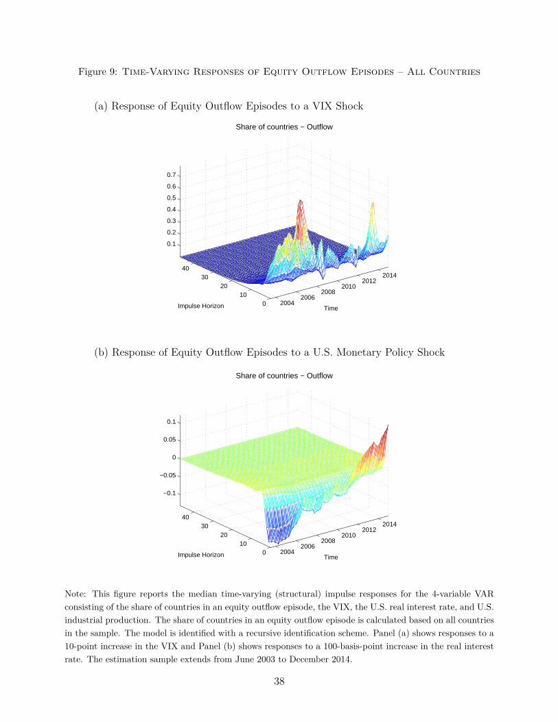
Figure 9: Time-Varying Responses of Equity Outflow Episodes – All Countries

(a) Response of Equity Outflow Episodes to a VIX Shock

20042006

20082010

20122014

010

2030

40

0.1

0.2

0.3

0.4

0.5

0.6

0.7

Time

Share of countries − Outflow

Impulse Horizon

(b) Response of Equity Outflow Episodes to a U.S. Monetary Policy Shock

20042006

20082010

20122014

010

2030

40

−0.1

−0.05

0

0.05

0.1

Time

Share of countries − Outflow

Impulse Horizon

Note: This figure reports the median time-varying (structural) impulse responses for the 4-variable VARconsisting of the share of countries in an equity outflow episode, the VIX, the U.S. real interest rate, and U.S.industrial production. The share of countries in an equity outflow episode is calculated based on all countriesin the sample. The model is identified with a recursive identification scheme. Panel (a) shows responses to a10-point increase in the VIX and Panel (b) shows responses to a 100-basis-point increase in the real interestrate. The estimation sample extends from June 2003 to December 2014.

38

Figure 10: Time-Varying Responses of Equity Outflow Episodes – Emerging Markets

(a) Response of Equity Outflow Episodes to a VIX Shock

20042006

20082010

20122014

010

2030

40

0

0.5

1

Time

Share of countries − Outflow

Impulse Horizon

(b) Response of Equity Outflow Episodes to a U.S. Monetary Policy Shock

20042006

20082010

20122014

010

2030

40

−0.2

−0.1

0

0.1

0.2

Time

Share of countries − Outflow

Impulse Horizon

Note: This figure reports the median time-varying (structural) impulse responses for the 4-variable VARconsisting of the share of countries in an equity outflow episode, the VIX, the U.S. real interest rate, andU.S. industrial production. The share of countries in an equity outflow episode is calculated based on allemerging markets in the sample. The model is identified with a recursive identification scheme. Panel (a)shows responses to a 10-point increase in the VIX and Panel (b) shows responses to a 100-basis-point increasein the real interest rate. The estimation sample extends from June 2003 to December 2014.

39

Figure 11: Time-Varying Responses of Equity Inflow Episodes – All Countries

(a) Response of Equity Inflow Episodes to a VIX Shock

20042006

20082010

20122014

010

2030

40

−1

−0.5

0

0.5

Time

Share of countries − Inflow

Impulse Horizon

(b) Response of Equity Inflow Episodes to a U.S. Monetary Policy Shock

20042006

20082010

20122014

0

10

20

30

40

−0.15

−0.1

−0.05

0

0.05

Time

Share of countries − Inflow

Impulse Horizon

Note: This figure reports the median time-varying (structural) impulse responses for the 4-variable VARconsisting of the share of countries in an equity inflow episode, the VIX, the U.S. real interest rate, and U.S.industrial production. The share of countries in an equity inflow episode is calculated based on all countriesin the sample. The model is identified with a recursive identification scheme. Panel (a) shows responses to a10-point increase in the VIX and Panel (b) shows responses to a 100-basis-point increase in the real interestrate. The estimation sample extends from June 2003 to December 2014.

40

Table1:

Results

oftheRegim

e-Sw

itching

Mod

el

Equity

Bon

d

Average

Adv

anced

Emerging

U.S.

Brazil

Average

Adv

anced

Emerging

U.S.

Brazil

µ1

-0.350

-0.110

-0.481

-0.072**

-0.339**

-0.588

-0.508

-0.626

-0.248**

-0.660**

[0.029]

[0.036]

[0.033]

[0.083]

µ2

0.030

0.008

0.041

0.016

0.135**

0.162

0.098

0.192

0.055**

0.057

[0.010]

[0.030]

[0.016]

[0.038]

µ3

0.513

0.250

0.658

0.275*

0.529**

0.736

0.563

0.817

0.323**

0.649**

[0.143]

[0.076]

[0.013]

[0.037]

p11

0.857

0.941

0.812

0.982

0.896

0.871

0.860

0.877

0.940

0.884

p22

0.905

0.916

0.899

0.987

0.889

0.905

0.906

0.904

0.942

0.884

p33

0.886

0.910

0.873

0.966

0.890

0.919

0.934

0.911

0.957

0.936

P(S

t=

1)0.306

0.348

0.283

0.320

0.366

0.245

0.242

0.246

0.291

0.209

P(S

t=

3)0.248

0.301

0.218

0.109

0.251

0.280

0.269

0.286

0.233

0.429

Note:

Thistablepresents

theestim

ationresults

(i.e.,b

ased

onEq

uatio

n(1))

ofthecoun

try-specificregime-sw

itching

mod

elsforequity

andbo

nd

fund

flowssepa

rately.The

results

show

nin

thetableconsist

oftheaverageresults

basedon

theentir

esample,

thead

vanced

coun

trysamplean

dthe

emerging

marketsample,

aswella

sthecoun

try-specificresults

fortheUnitedStates

andforBrazil.µ

1,µ

2an

dµ

3aretheintercepts

forthethree

regimes.p

11is

thetran

sitionprob

ability

ofstayingin

thefirst

regime(i.e.,t

hestrong

outflow

regime),p

22is

thetran

sitionprob

ability

ofstaying

inthesecond

regime(i.e.,t

he“n

ormal”regime)

andp

33is

thetran

sitionprob

ability

ofstay

ingin

thethird

regime(i.e.,t

hestrong

inflo

wregime).

P(S

t=

1)is

theun

cond

ition

alprob

ability

ofbe

ingin

thefirst

regimean

dP

(St

=3)

istheun

cond

ition

alprob

ability

ofbe

ingin

thethird

regime.

Forthesix

coun

try-specificintercepts,w

ealso

providestan

dard

errors

inbrackets.The

stan

dard

errors

arecalculated

from

theinverseof

theou

ter

prod

uctestim

ateof

theHessia

n.**,*

indicate

statist

ical

significan

ceat

the5pe

rcentan

d10

percentlevel,respectiv

ely.

41

Table 2: Summary Results: Characterizing Capital Flow Regimes

Panel A: Descriptive Statistics

Equity Outflows Avg. Probability Avg. Share in Episode Frequency Avg. Length

All Countries 0.304 0.261 12.785 17.421Advanced 0.349 0.332 9.261 30.248Emerging 0.279 0.221 14.714 10.397

Equity Inflows Avg. Probability Avg. Share in Episode Frequency Avg. Length

All Countries 0.250 0.230 9.908 20.020Advanced 0.306 0.294 9.130 26.522Emerging 0.220 0.195 10.333 16.459

Bond Outflows Avg. Probability Avg. Share in Episode Frequency Avg. Length

All Countries 0.239 0.211 7.303 16.831Advanced 0.233 0.195 5.619 21.216Emerging 0.242 0.218 8.089 14.784

Bond Inflows Avg. Probability Avg. Share in Episode Frequency Avg. Length

All Countries 0.281 0.268 7.985 19.010Advanced 0.272 0.262 5.905 23.260Emerging 0.285 0.271 8.956 17.026

Panel B: Selected Correlations

Equity Outflows vs. Bond Outflows Equity Inflows vs. Bond Inflows

All countries 0.358 0.175Advanced 0.274 0.049Emerging 0.417 0.259

Note: “Avg. Probability” is the average probability of being in a strong inflow or strong outflow regime,

which is obtained from the regime-switching model (see Equation (1)). “Avg. Share in Episode” is the average

percent of time a country spends in an inflow or an outflow episode, where an episode is identified if the

probability of being in a strong inflow or strong outflow regime is higher than 0.5 for at least four consecutive

weeks. “Frequency” is the frequency with which inflow or outflow episodes appear, and “Avg. Length” is the

average number of weeks spent in an inflow or outflow episode. Panel B reports the correlation coefficient

between equity outflow (inflow) and bond outflow (inflow) episodes.

42