The Dynamic and Stochastic Shortest Path

Problem with Anticipation 1

Barrett W. Thomas ∗

Dept. of Management Sciences, University of Iowa, Iowa City, IA 52242-1000

Chelsea C. White III

Dept. of Industrial and Systems Engineering, Georgia Institute of Technology,

Atlanta, GA 30332-0205

Abstract

Mobile communication technologies enable truck drivers to keep abreast of changing

traffic conditions in real-time. We assume that such communication capability ex-

ists for a single vehicle traveling from a known origin to a known destination where

certain arcs en route are congested, perhaps as the result of an accident. Further,

we know the likelihood, as a function of congestion duration, that congested arcs

will become uncongested and thus less costly to traverse. Using a Markov decision

process , we then model and analyze the problem of constructing a minimum ex-

pected total cost route from an origin to a destination that anticipates and then

responds to changes in congestion, if they occur, while the vehicle is en route. We

provide structural results and illustrate the behavior of an optimal policy with sev-

eral numerical examples and demonstrate the superiority of an optimal anticipatory

policy, relative to a route design approach that reflects the reactive nature of current

routing procedures.

Preprint submitted to Elsevier Science 3 October 2005

Key words: routing, real-time decision making, Markov decision processes.

1 Introduction

In the past decade, the combination of real-time traffic information and in-

vehicle communication technology has given drivers the ability to route them-

selves in coordination with changing traffic conditions. The ability to avoid

traffic congestion is particularly important for drivers operating in a just-in-

time delivery environment. For example, a trucking company can be penalized

thousands of dollars per minute if a late shipment causes an assembly line to

shut down at an auto plant [1]. Recent research has recognized the importance

of these problems through time-dependent or real-time and stochastic short-

est path problems. This research typically assumes that the level of congestion

changes according to the time of day or that changes are observed, but are not

based on the length of time a road segment has been congested. In this paper,

we consider the case where the congestion dissipates over time according to

some known probability distribution. This case is the result of an accident or

some other unique or relatively rare event whose occurrence is hard to predict,

but whose end is governed by such a probability distribution. For example, in

∗ Corresponding author.Email address: barrett-thomas@uiowa.edu (Barrett W. Thomas).

1 The authors express their appreciation to the Alfred P. Sloan Foundation and

the Trucking Industry Program (TIP) for supporting the research presented in this

paper. TIP is part of the Sloan Industry Centers Network. We are also grateful to

James Bean, Mark Lewis, Demosthenis Teneketzis, and three anonymous referees

for their helpful suggestions.

2

the event of an accident, the more time that has passed since the accident,

the more likely it is that emergency crews have arrived and are cleaning up

the accident scene, getting traffic flowing again. As another example, consider

United States’ border crossings. In this case, traffic backups can result when a

particular vehicle requires additional security checks. The more time that has

elapsed since this check was begun, the more likely that the check will end.

One way to overcome the congestion caused by one of these unique traffic

events would be to re-route around the congested road segments. However,

simply re-routing around traffic congestion or security delays could take the

vehicle on an out-of-the-way and potentially much more expensive route. If

the real-time traffic information is coupled with distributions on the amount

of time that the particular road segments spend in each state of congestion

or delay, the driver can geographically position the vehicle so as to be able to

anticipate changes in the status of road segments. This ability to anticipate

motivates the following problem.

Consider a single vehicle that is to travel on a known road network from a

fixed origin to a fixed destination. The vehicle accrues a cost for each arc

that is crossed en route to the destination, and this cost is arc dependent and

stochastic. For a fixed cost, the driver also has the option of waiting at the

current location. There exists a subset of arcs whose level of congestion is

observable and for which the travel time is also dependent on the condition

of the arc. For example, the travel-time distribution changes with regard to

whether or not traffic on the arc is free flowing or has been slowed by an

accident. We assume that the driver knows instantaneously if the status of one

of these observed arcs has changed. In addition, if an arc is congested due to an

accident or some other event, there is a known distribution on the likelihood

3

of the status of an observed arc transitioning from the congested state to an

uncongested state. This distribution is parameterized by the amount of time

that the observed arc has spent in its congested state and is assumed to follow

the increasing failure rate property. The problem objective is to determine a

policy for selecting a path that minimizes the expected total cost of the trip

from origin to destination.

We emphasize that this paper is not focused on traffic congestion that results

from typical “rush hours” or on traffic congesting events whose origins are

unidentifiable, but rather on those events whose duration is stochastic and

whose distribution depends on the amount of time that has elapsed since

the event occurred. Further, we assume that these congesting events, such as

accidents or security delays, are relatively rare and hence will assume that

we cannot predict the occurrence of these events. Computational experience

demonstrates that when these events are highly unlikely, they have no effect

on the optimal policy nor on the expected cost [see [2]]. Thus, we will focus on

the case where such events have already occurred and where the uncongested

case is a trapping state.

As an example of the described problem, consider a vehicle that leaves a known

origin for a known destination, where the destination must be reached before

some prespecified future time. Suppose that the driver of the vehicle knows

that there is an accident along the preferred path from origin and destination.

Intuitively, it seems reasonable that, as a result of the congestion, the driver

may want to consider an alternate route. However, if the driver knows a prob-

ability distribution on the duration of the congestion, the driver may find that

it is still better to follow the preferred path in anticipation of the congestion

clearing. At the same time, incorporating probabilities on the status of the

4

observed arc might produce a routing policy such that the route actually goes

somewhere in between the extremes of preferring the congested arc and avoid-

ing it altogether. In this way, the vehicle might be better positioned to divert

to the particular arc if the arc’s status changes in a cost-improving way. Such a

path would anticipate the change in the arc’s status. Hence, we call this prob-

lem the dynamic and stochastic shortest path problem with anticipation.

This paper is outlined as follows. In Section 2, we present a review of the

relevant literature. Section 3 establishes a Markov decision process model for

the problem with Section 4 providing the optimality equations and prelimi-

nary results for the model. In Section 5, we explore the structure of the cost

function and optimal policy. Section 6 offers visual examples of optimal antici-

patory policies. In Section 7, we characterize a non-anticipating policy. Section

8 explains the design of the numerical experiments intended to empirically de-

scribe the performance of anticipatory routing and to determine the value of

anticipatory information relative to the non-anticipating policy, with Section

9 presenting the results of these experiments. Section 10 provides concluding

remarks.

2 Literature Review

As the name of this paper suggests, this research falls under the broad category

of dynamic and stochastic shortest path problems. The problems are dynamic

in the sense that the cost of traversing arcs can change over the problem hori-

zon. In general, the only stochasticity in shortest path problems results from

decision makers having probabilistic information about the time required to

traverse an arc. For generality, our model maintains stochastic travel times, but

5

we focus on another stochastic element associated with the dynamic changes

in arc cost. We assume that certain arc-cost distributions themselves change

according to a known probability distribution. To distinguish the two types

of stochastic elements, we refer to the probabilistic information on the dura-

tions of congestion as anticipatory information. In the rest of this section, we

present an overview of related literature. To limit the scope of the review, we

have focused our attention to dynamic and stochastic shortest path problems,

and the vehicle routing analogy, the dynamic and stochastic routing problem.

Initial work in stochastic and dynamic shortest paths was done by Hall [3] who

introduced the stochastic, time-dependent shortest path problem (STDSPP).

In the STDSPP, travel times on arcs are stochastic and the travel-time dis-

tributions on these arcs are known and time-dependent. Hence, the times at

which arc travel time distributions transition is known in advance. Hall showed

that the optimal policy is “adaptive.” That is, the optimal actions are subject

not only to the vehicle’s location, but also to the time at which the vehicle is

at the location. In this way, the policy accounts for the time dependency of

the travel-time distributions. Bander and White [4] demonstrate the compu-

tational effectiveness of the heuristic search algorithm AO* on the STDSPP.

Fu and Rilett [5] extend Hall’s work to the case of continuous-time random arc

costs. Miller-Hooks and Mahmassani [6] present and compare algorithms for

the least possible cost path in the discrete-time STDSPP. Miller-Hooks and

Mahmassani [7] provide an algorithm for finding the least expected cost path

in the discrete-time STDSPP. Chabini [8] provides an optimal run-time algo-

rithm for a variation of the STDSPP in which arc costs are time dependent,

but not stochastic.

Polychronopoulos and Tsitsiklis [9] relax the assumption on time-dependent

6

arc cost transitions and introduce the dynamic shortest path problem (DSPP).

In the DSPP, arc costs are randomly distributed, but the realization of the

random arc costs becomes known once the vehicle arrives at the arc. Cheung

[10] provides an iterative algorithm for a similar DSPP. Cheung and Muralhid-

haran [11] use DSPP in the development of an adaptive algorithm for routing

priority shipments in the less-than-truckload trucking industry. Psaraftis and

Tsitsiklis [12] discuss another variation of the DSPP in which the distribu-

tions on arc travel times evolve over time according to a Markov process.

However, unlike the work presented in this paper, the changes in the status

of the arc are not observed until the vehicle reaches the arc. We note that, in

their conclusions, Psaraftis and Tsitsiklis and Polychronopoulos and Tsitsiklis

suggest a problem similar to the one being considered in this paper. Davies

and Lingras [13] propose a genetic algorithm for dynamically rerouting in a

situation similar to [12] in which the arc cost distributions are a function of

time, but these distributions become known only as that time arrives. Waller

and Ziliaskopoulos [14] develop algorithms for problems with limited spatial

and temporal arc dependencies.

Kim, Lewis, and White [15] extend [12] to include real-time information. They

model the problem in a manner similar to that presented in this paper (al-

though they do not consider the amount of time that an observed arc has

spent in a particular state) and present results regarding optimal departure

times from a depot and optimal routing policies. Kim, Lewis, and White [16]

present a state-space reduction technique that significantly improves compu-

tation time for the problem introduced in [15]. Azaron and Kianfar [17] extend

the analytical results shown in [12] for the case where the states of the current

arc and immediately adjacent arcs are known. Azaron and Kianfar also show

7

an example of a problem similar to that presented in this work. However, they

offer no analytical results and the example is too small to show how a vehicle

benefits from anticipating changes on its route. Rather than congestion clear-

ing as is the case in this research, Ferris and Ruszcznski [18] present a problem

in which arcs can fail and become unusable. Ferris and Ruszcznski model the

problem as an infinite-horizon Markov decision process similar to stochastic

shortest path formulations in [19] and provide an example that illustrates the

behavior of the optimal policy.

In this paper, we define anticipation to mean that we have known probability

distributions that are dependent on the amount of time spent in a particular

state. Anticipation in this context has been considered in only a few works.

Powell et al. [20] introduce a truckload dispatching problem, and Powell [21]

provides formulations, solution methods, and numerical results. In these pa-

pers, future demand forecasts are used to determine which loads should be

assigned to what vehicles in a truckload environment in order to account for

forecasted capacity needs in the next period. Extending Datar and Ranade

[22] in which bus arrival times are exponentially and independently distrib-

uted, Boyan and Mitzenmacher [23] provide a polynomial-time algorithm for

the problem of traversing a bus network in which bus-arrival times are dis-

tributed according to a probability distribution with the increasing failure

rate property. The distributions on bus-arrival times are analogous to the dis-

tribution on the duration of congestion presented in this research. Thomas

and White [24] consider a problem analogous to the problem presented here

in which customer service requests are anticipated instead of changes in the

status of arcs. In [24], each customer has a known distribution on the time

of day that the customer is likely to request service and the optimal policy

8

geographically positions the vehicle to respond to requests in a manner that

minimizes expected total cost.

3 Model Formulation

In this section, we present a Markov decision model for the dynamic and

stochastic shortest path problem with anticipation. Let the graph G = (N, E)

serve as a model of the road network, where N is the finite set of nodes,

modeling intersections, and E ⊆ N × N is the set of arcs, modeling one-

way roads between intersections. The arc (n, n′) ∈ E if and only if there is

a road that permits traffic to flow from intersection n to intersection n′. Let

SCS(n) = {n′ : (n, n′) ∈ E} be the successor set of n ∈ N . We assume

n ∈ SCS(n). Let s ∈ N be the origin, or start node, of the trip, and let γ ∈ N

be the destination, or goal node, of the trip. We assume SCS(γ) = γ. Let

the set EI = {e1, . . . , eL} ⊆ E be the set of observed arcs, where L = |EI |

and |EI | is the cardinality of EI . Each element of EI represents an one-way

road for which we can observe congestion, and if congestion occurs, we know

a probability distribution on the duration of the congestion.

We assume that there exists a path to γ from every n ∈ N . A path p from n1

to nj in N is a sequence of nodes {n1, n2, · · · , nj−1, nj} such that n1, · · · , nj

are in N and (nr, nr+1) ∈ E for r = 1, · · · , j − 1. Let P(n) be the set of all

paths from n to γ.

A decision epoch occurs when the vehicle arrives at a node. Let tq be the time

of the qth decision epoch, and let nq ∈ N be the position of the vehicle at time

tq. Then, t1 = 0 and n1 = s. Let T be a finite integer indicating that action

9

selection terminates at a time no later than T −1. T might represent the time

by which the vehicle is supposed to fulfill its pick-up or delivery obligations.

For all q, we assume tq ∈ {1, . . . , T}. Let the random variable Q be such that

tQ < T and tQ+1 ≥ T , where tQ and tQ+1 are realizations of the random

variables tQ and tQ+1. We remark that tQ+1−T is the amount of time beyond

the delivery deadline required for the vehicle to make its pick-up or delivery.

Assume that the information infrastructure is such that we know the status

of each arc e ∈ EI . We let K l(t) be a random variable representing the state

of arc el ∈ EI at time t. Then, the status of the observed arcs is given by the

vector K(t) = {K1(t), . . . , KL(t)} where

K l(t) =

1 if arc el is congested

2 if arc el is not congested.

We denote realizations of K l(t) and K(t) as kl and k, respectively. We assume

that the information infrastructure is such that the driver knows instanta-

neously when the status of arc el ∈ EI , l = 1, . . . , L, has changed.

In addition, we assume that the information infrastructure tracks the amount

of time that each arc in EI has spent in its current state if the current state is

congested. We let X l(t) be the number of time units that arc el has been in its

current state K l(t). We represent a realization of X l(t) by xl and assume 0 ≤

xl ≤ X, where X < ∞, for all l. If arc el is in an uncongested state, K l(t) = 2,

we let xl = 0 because in this the uncongested state xl has no effect on the

cost or probability calculations. Then, X(t) = {x1, . . . , xL} ∈ {1, . . . ,X}L. A

realization of X(t) is denoted by x.

10

We model the transition of observed arcs from congested to noncongested

as discrete-time Markov chains. We recognize that these transitions actually

occur in continuous time. However, in our model, decision epochs occur when

the vehicle reaches an intersection and not when a transition occurs at an

observed arc. To be consistent with our model of arc travel times, we then

approximate the time of observed arc transitions using a discrete-time model.

Given the congestion causing events being discussed in this paper are rela-

tively rare, such as accidents, the congestion on one arc is unlikely to imply

congestion on another. Formally, we then make the following assumption.

Assumption 1 {Ki(t), t = 0, 1, . . . , T} and {Kj(t), t = 0, 1, . . . , T} are in-

dependent Markov chains for i 6= j.

Further, because congesting causing events are relatively rare and unlikely

to occur while the vehicle is en route, we consider the uncongested state a

trapping state. We note that, in the event that a congesting causing event

occurs during the problem horizon, we can solve the new problem by simply

resolving the problem letting our current position be the start node.

Given these assumptions, for each arc el ∈ EI , we assume that the state

dynamics for kl = 1 and xl are described by the one-step transition matrix:

Rl(x,x+1) =

1− αl

x αlx

0 1

,

where αlx is the probability that, having been in state kl = 1 for x time units,

arc el transitions from kl = 1 to (kl)′ = 2 in one time unit. We also make the

following assumption on the nature of αlx.

11

Assumption 2 Let αlx ≤ αl

x′ for all l and for all xl and (xl)′ such that xl ≤

(xl)′.

This condition is equivalent to assuming that the distribution on congestion

duration has an increasing failure rate property (IFR)[25]. Intuitively, the IFR

property says that the longer an arc has been congested, the more likely it

is that the congestion will clear. This assumption reflects our desire to model

congestion resulting from accidents or security delays rather than from the

time-dependent congestion resulting from “rush hours.” The IFR property is

frequently used in reliability theory to represent the fact that, the more a

machine is used, the more likely it is to fail. For additional discussion of the

IFR property, see [25] and [26].

Let P (k′ | t, k, x, t′) be the probability of a transition occurring from k at time

t with x units of time in state k to k′ at time t′ > t. By our assumptions,

P (k′ | t, k, x, t′) = P (K(t′) = k′ | k(t) = k, X(t) = x)

=L∏

l=1

P (K l(t′) = (kl)′ | K l(t) = kl),

where each term in the product satisfies an extension of Kolmogorov’s equa-

tions for the non-stationary case [see Kim, Lewis, and White [15]] such that

Rl(x,x′) =

1− αl

x αlx

0 1

×

1− αlx+1 αl

x+1

0 1

× · · · ×

1− αlx′−1 αl

x′−1

0 1

.

The state of the dynamic and stochastic shortest path problem with anticipa-

tion is (n, t, k, x), where n is the location of the vehicle at time t, k(t) = k, and

x(t) = x. The state dynamics are described by the conditional probability:

12

P (t′, k′ | n, t, k, x, n′) = P (t′ | n, t, k, n′)P (k′ | t, k, x, t′),

where P (t′ | n, t, k, n′) is the probability that a vehicle leaving node n at time

t will arrive at node n′ at time t′ > t, assuming k(t) = k and that the vehicle

travels on arc (n, n′) ∈ E.

We make two assumptions with regard to P (t′ | n, t, k, n′).

Assumption 3 Let P (t′ | n, t, k, n′) be stationary in t and remark that P (t′ |

n, t, k, n′) depends on k only if (n, n′) = el ∈ EI , and then only on kl.

Our second assumption describes the relationship between travel time and

congestion.

Assumption 4 If (n, n′) = el ∈ EI and kl < kl, then, for all λ ∈ {1, 2, . . .},

∑t′≤λ

P (t′ | n, t, k, n′) ≥∑t′≤λ

P (t′ | n, t, k, n′).

Assumption 4 implies that (t′ − t | n, kl, n′) stochastically dominates (t′ − t |

n, kl, n′), where (t′ − t | n, kl, n′) and (t′ − t | n, kl, n′) are random variables

representing the amount of time required to traverse arc (n, n′) = el when in

states kl and kl, respectively. Essentially, stochastic dominance implies that a

congested arc is likely to take a longer time to cross than an uncongested arc.

For additional discussion of stochastic dominance, see [27]. We also assume

that there exists some β such that, for all n, t, k, and n′, P (t′ | n, t, k, n′) = 0

for all t′ such that t′− t > β. Finally, we assume P (t+1 | n, t, k, n) = 1. Thus,

if the action chosen when at node n is to stay at node n, then the driver must

wait 1 time unit before making another decision.

The action set is A(n) = SCS(n). Thus, when at node n at time t, K(t) = k,

13

and X(t) = x, the driver chooses the next node to which to travel. We remark

that |SCS(n)| is necessarily finite.

A decision rule at time t is a function δ(·, t, ·, ·) : N ×{1, 2}L×{1, . . . , X}L →

A(n) that selects an available action at each time t. Thus, δ(n, t, k, x) ∈ A(n).

A policy is a sequence of decision rules π = {δ(·, 1, ·, ·), δ(·, 2, ·, ·), . . . , δ(·, T −

1, ·, ·)}. We remark that δ(·, t, ·, ·) is implemented only if t is a decision epoch.

The cost structure is composed of travel costs between nodes. Let c(n, t, k, x, a) =

c(n, t, k, a) be the expected cost to be accrued between decision epochs q and

q + 1, given the vehicle is currently at node n(tq) = n, tq = t, K(tq) = k,

X(tq) = x, and a ∈ A(n). For a = n′ and tq+1 = t′ being the time of arrival at

node n′,

c(n, t, k, n′) =∑t′

P (t′ | n, t, k, n′)c(t′ − t),

where c(t) is the cost of traveling for t units of time and where the strictly

positive function c is non-decreasing in t. We assume c(t) < ∞ for all t < ∞.

We define k ≤ k if and only if kl ≤ kl for all l. Then, Assumption 4 implies

that c(n, t, k, a) ≥ c(n, t, k, a) for all k ≤ k [see [27], p. 405]. We assume

c(γ, t, k, γ) = 0 for all t and k. We assume the terminal cost, i.e., nQ+1 6= γ,

accrued is c(nQ+1, tQ+1). For nQ+1 6= γ, we let c(nQ+1, tQ+1) = c(nQ+1, tQ+1)+

c(nQ+1, tQ+1). We also make the following assumption.

Assumption 5 For every t > T , we define c(n, t) ≥ minp(n)∈P(n) cβ(p(n)),

where cβ(p(n)) is the cost of the path p(n) with all arcs requiring β units of

time to traverse.

In reality, the penalty associated with missing service obligations at time T

would likely be much larger than c [see [1]]. Our definition of c simply reflects

14

the minimum requirement of our structural results. We let c(nQ+1, tQ+1) be

the cost associated with the amount of time by which the time horizon was

violated. We assume t′ ≤ t′′ implies 0 < c(n, t′) ≤ c(n, t′′), and for all t such

that t− T ≤ β, c(n, t) ≤ β for all n. Thus, the earlier we terminate after time

T , the better.

Let

fπ(s, 1, k, x) = Eπk,x{

Q∑q=1

c(nq, tq, kq, xq, aq) + c(nQ+1, tQ+1)}

be the problem criterion, where Eπk,x is the expectation operator, conditioned

on the use of policy π, K(1) = k, and X(1) = x. The problem objective

is to find a policy π?, called an optimal policy, such that fπ?(s, 1, 1, 0) ≤

fπ(s, 1, 1, 0) for all policies π and for all k and x.

4 Optimality Equations and Preliminary Results

All of the results in this section can be found in [Puterman [28], section 4.3].

The optimality equation is

f(n, t, k, x) = min{c(n, t, k, x, a) +∑

t′,k′,x′P (t′ | n, t, k, a)

×P (k′ | t, k, x, t′)P (x′ | t, k, x, t′, k′)f(a, t′, k′, x′) : a ∈ A(n)},

where f(n, t, k, x) = c(n, t) for T ≤ t ≤ T + β. The solution of the optimality

equation is unique, and f(n, t, k, x) = minπ fπ(n, t, k, x), for all n, t, k, and

x. We refer to f(n, t, k, x) as the cost or cost-to-go function. A necessary and

sufficient condition for π? to be optimal is that it is composed of decision rules

that cause the minimum in the optimality equation to hold.

15

Notationally, it will be useful to make the dependence of f(n, t, k, x) explicit

on Px, where Px = {P (· | t, k, x′) : x′ ≥ x} and P (· | t, k, x′) = {P (t′ − t |

k, x′) : t′ > t}. Then, Px is a vector in which each component is itself a

vector of probabilities. This notation will allow us to differentiate between

different distributions on amount of time that arcs remain congested. Note,

Px = {P (· | t, k, x), Px+1}. Thus, we will occasionally refer to f(n, t, k, x) as

f(n, t, k, x, Px).

5 Structural Results on the Cost Function and Optimal Policy

In this section, we present the structural results on the cost function and

on the optimal policy for the dynamic and stochastic shortest path problem

with anticipation. These results imply that there exist conditions under which

the current optimal policy remains optimal when problem data changes. In

addition, the results offer the practitioner an improved intuitive understanding

of the behavior of the cost function and the optimal policy. We will first present

a useful result, proof of which can be found in Puterman [28], p. 106.

Lemma 1 Let {pj} and {p′j} be real-valued non-negative sequences satisfying

∞∑j=k

pj ≥∞∑

j=k

p′

j (1)

for all k, with equality holding for k = 0. Suppose vj+1 ≥ vj for j = 1, . . . ,

then

∞∑j=0

pjvj ≥∞∑

j=0

p′

jvj, (2)

where the limits exist but may be infinite.

16

Equation 1 is equivalent to the statement that pj stochastically dominates p′j.

Thus, the consequence of the lemma, Equation 2, is the expected value of v is

greater under the distribution given by {pj} than by {p′j}.

We now present inequalities on the cost function. Our first result implies that

the sooner we reach any intersection, the less the expected future cost. This

result is important for future results related to the value function and the arc

status vector k.

Theorem 1 Given Assumptions 3 and 5, the cost function f(n, t, k, x) is non-

decreasing in t for all n, k, and x.

Proof: The result holds by Assumption 5 for all n, k, x and for any t and

all t′ such t < t′ and t′ ≥ T . We assume that the result holds for all n, k, x

and for all t′′ and t′ such that t′′ < t′ and t′′ > t. We note that Assumption

3 implies P (t + a | n, t, k, n′) = P (t′ + a | n, t′, k, n′) for all n, t, t′, k, n′, and

a, P (k′ | t, k, x, t + a) = P (k′ | t′, k, x, t′ + a) for all t, t′, k, x, k′, and a, and

P (x′ | t, k, x, t + a, k′) = P (x′ | t′, k, x, t′ + a, k′) for all t, t′, k, x, k′, x′, and a.

Then, assuming t′ ≥ t,

f(n, t, k, x) = minn′{c(n, t, k, n′) +

∑a

P (t + a | n, t, k, n′)

×∑k′

∑x′

P (k′ | t, k, x, t + a)f(n′, t + a, k′, x′)

≤minn′{c(n, t′, k, n′) +

∑a

P (t′ + a | n, t′, k, n′)

×∑k′

∑x′

P (k′ | t′, k, x, t′ + a)f(n′, t′ + a, k′, x′)

= f(n, t′, k, x),

where the inequality follows from the induction hypothesis.

17

The next result presents inequalities associated with the status of the observed

arcs. In the L = 1 case, it is intuitive that the more improved the status of

the observed arc, the less cost associated with traversing the network. Recall

that k ≤ k if and only if kl ≤ kl for all l.

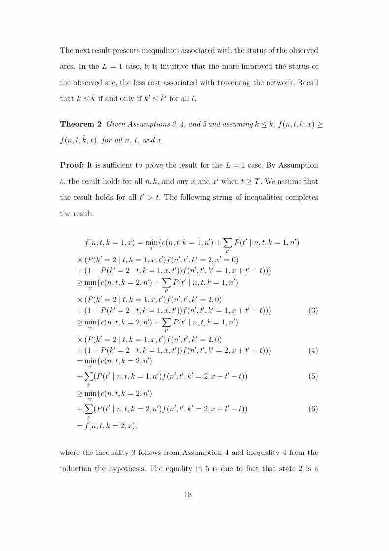
Theorem 2 Given Assumptions 3, 4, and 5 and assuming k ≤ k, f(n, t, k, x) ≥

f(n, t, k, x), for all n, t, and x.

Proof: It is sufficient to prove the result for the L = 1 case. By Assumption

5, the result holds for all n, k, and any x and x′ when t ≥ T . We assume that

the result holds for all t′ > t. The following string of inequalities completes

the result:

f(n, t, k = 1, x) = minn′{c(n, t, k = 1, n′) +

∑t′

P (t′ | n, t, k = 1, n′)

× (P (k′ = 2 | t, k = 1, x, t′)f(n′, t′, k′ = 2, x′ = 0)

+ (1− P (k′ = 2 | t, k = 1, x, t′))f(n′, t′, k′ = 1, x + t′ − t))}≥min

n′{c(n, t, k = 2, n′) +

∑t′

P (t′ | n, t, k = 1, n′)

× (P (k′ = 2 | t, k = 1, x, t′)f(n′, t′, k′ = 2, 0)

+ (1− P (k′ = 2 | t, k = 1, x, t′))f(n′, t′, k′ = 1, x + t′ − t))} (3)

≥minn′{c(n, t, k = 2, n′) +

∑t′

P (t′ | n, t, k = 1, n′)

× (P (k′ = 2 | t, k = 1, x, t′)f(n′, t′, k′ = 2, 0)

+ (1− P (k′ = 2 | t, k = 1, x, t′))f(n′, t′, k′ = 2, x + t′ − t))} (4)

= minn′{c(n, t, k = 2, n′)

+∑t′

(P (t′ | n, t, k = 1, n′)f(n′, t′, k′ = 2, x + t′ − t)) (5)

≥minn′{c(n, t, k = 2, n′)

+∑t′

(P (t′ | n, t, k = 2, n′)f(n′, t′, k′ = 2, x + t′ − t)) (6)

= f(n, t, k = 2, x),

where the inequality 3 follows from Assumption 4 and inequality 4 from the

induction the hypothesis. The equality in 5 is due to fact that state 2 is a

18

trapping state and how long we have been in the trapping state has no effect

on future costs. The inequality in 6 follows from Lemma 1 and Theorem 1.

We now show that the longer that an arc has been congested, the less the

expected total cost-to-go. We say x ≤ x if and only if xl ≤ xl for all l.

Theorem 3 Given Assumptions 2 and 5, when x ≤ x, f(n, t, k, x) ≤ f(n, t, k, x)

for all n, t, and k.

Proof: It is sufficient to prove the result for the L = 1 case. By Assumption

5, the result holds for all n, k, and x and x′ such that x ≤ x′ when t ≥ T . We

assume that the result holds for all t′ > t. To complete the proof, we have the

following string of inequalities:

f(n, t, k = 1, x) = minn′{c(n, t, k = 1, n′) +

∑t′

P (t′ | n, t, k = 1, n′)

× (P (k′ = 2 | t, k = 1, x, t′)f(n′, t′, k′ = 2, x′′ = 0)

+ (1− (P (k′ = 2 | t, k = 1, x, t′))f(n′, t′, k′ = 1, x + t′ − t))}≥min

n′{c(n, t, k = 1, n′) +

∑t′

P (t′ | n, t, k = 1, n′)

× (P (k′ = 2 | t, k = 1, x, t′)f(n′, t′, k′ = 2, 0)

+ (1− (P (k′ = 2 | t, k = 1, x, t′))f(n′, t′, k′ = 1, x + t′ − t))}≥min

n′{c(n, t, k = 1, n′) +

∑t′

P (t′ | n, t, k = 1, n′)

× (P (k′ = 2 | t, k = 1, x, t′)f(n′, t′, k′ = 2, 0)

+ (1− (P (k′ = 2 | t, k = 1, x, t′))f(n′, t′, k′ = 1, x + t′ − t))}= f(n, t, k = 1, x),

where the first inequality follows from our Assumption 2 and Theorem 2.

Induction completes the proof.

We will now show that the more likely an arc is to become uncongested, the

more likely that costs will be reduced. We also show that the cost function

is PLNIC. Recall, a real-valued function h on a linear vector space Y ⊆ <L

19

is PLNIC if and only if there is a finite set Γ ⊆ < × <L such that h(y) =

min{γ0m + γ1

my : (γ0m, γ1

m) ∈ Γ}, where γ1m ≤ 0 for all m. For two vectors y and

z of the same order, we define yz to be the usual vector dot product.

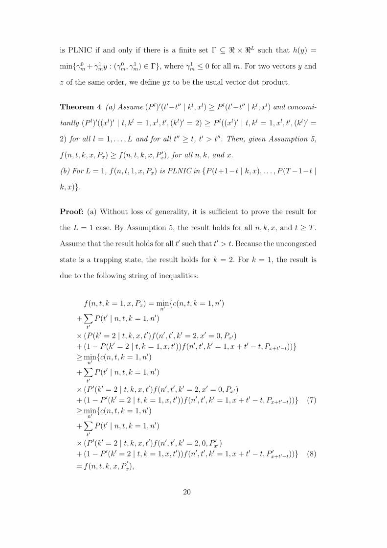
Theorem 4 (a) Assume (P l)′(t′−t′′ | kl, xl) ≥ P l(t′−t′′ | kl, xl) and concomi-

tantly (P l)′((xl)′ | t, kl = 1, xl, t′, (kl)′ = 2) ≥ P l((xl)′ | t, kl = 1, xl, t′, (kl)′ =

2) for all l = 1, . . . , L and for all t′′ ≥ t, t′ > t′′. Then, given Assumption 5,

f(n, t, k, x, Px) ≥ f(n, t, k, x, P ′x), for all n, k, and x.

(b) For L = 1, f(n, t, 1, x, Px) is PLNIC in {P (t+1−t | k, x), . . . , P (T−1−t |

k, x)}.

Proof: (a) Without loss of generality, it is sufficient to prove the result for

the L = 1 case. By Assumption 5, the result holds for all n, k, x, and t ≥ T .

Assume that the result holds for all t′ such that t′ > t. Because the uncongested

state is a trapping state, the result holds for k = 2. For k = 1, the result is

due to the following string of inequalities:

f(n, t, k = 1, x, Px) = minn′{c(n, t, k = 1, n′)

+∑t′

P (t′ | n, t, k = 1, n′)

× (P (k′ = 2 | t, k, x, t′)f(n′, t′, k′ = 2, x′ = 0, Px′)

+ (1− P (k′ = 2 | t, k = 1, x, t′))f(n′, t′, k′ = 1, x + t′ − t, Px+t′−t))}≥min

n′{c(n, t, k = 1, n′)

+∑t′

P (t′ | n, t, k = 1, n′)

× (P ′(k′ = 2 | t, k, x, t′)f(n′, t′, k′ = 2, x′ = 0, Px′)

+ (1− P ′(k′ = 2 | t, k = 1, x, t′))f(n′, t′, k′ = 1, x + t′ − t, Px+t′−t))} (7)

≥minn′{c(n, t, k = 1, n′)

+∑t′

P (t′ | n, t, k = 1, n′)

× (P ′(k′ = 2 | t, k, x, t′)f(n′, t′, k′ = 2, 0, P ′x′)

+ (1− P ′(k′ = 2 | t, k = 1, x, t′))f(n′, t′, k′ = 1, x + t′ − t, P ′x+t′−t))} (8)

= f(n, t, k, x, P′

x),

20

where inequality 7 follows from assumptions, Theorem 2, and Theorem 3, and

the inequality in 8 from the induction hypothesis.

(b) Recursively expanding the optimality equations for t′ = t+1 to t′ = T −1

and rearranging the terms, we get

f(n, t, k = 1, x, Px) = minn′{c(n, t, k, n) +

∑t≥T

c(n′, t′)

+T−1∑

t′=t+1

P (t′ | n, t, k, n′)f(n′, t′, k′ = 1, x + t′ − t, Px+t′−t)

+T−1∑

t′=t+1

P (t′ | n, t, k, n′)P (k′ = 2 | t, k = 1, x, t′)

× (∑x′

P (x′ | t, k = 1, x, t′, k′ = 2)[f(n′, t′, k′ = 2, x′, P ′x)

− f(n′, t′, k′ = 1, x + t′ − t, Px+t′−t)])}.

Clearly, the term within the brackets is linear in {P (t′ − t | k, x), t′ = t +

1, . . . , T−1} for each n′ ∈ SCS(n) and each term has a non-positive coefficient,

since P (t′ | n, t, n′) ≥ 0, and by Theorem 2, f(n′, t′, k = 2, x′Px′) ≤ f(n′, t′, k =

1, x + t′ − t, Px+t′−t) for all t′ > t and for any x′ and x + t′ − t. The minimum

of a finite number of such functions is PLNIC. Induction completes the proof.

We now use the inequalities on the value function to explore the structure of

the optimal policy. Our result, Corollary 1, indicates that an optimal decision

rule is invariant on convex sets of {P (· | t, k, x)} as long as {P (· | t, k, x′′ :

x′′ > x)} does not change. For the L = 1 case, this result suggests that

if δ?(n, t, k = 1, x, Px) = δ?(n, t, k = 2, x, Px) and δ?(n, t, k = 1, x, P ′x) =

δ?(n, t, k = 2, x, P ′x), then given P ′′(· | t, k, x) is a convex combination of P (· |

t, k, x) and P ′(· | t, k, x) and few additional restrictions are met, δ?(n, t, k =

1, x, P ′′x ) = δ?(n, t, k = 1, x, Px). That is, under certain conditions, the optimal

21

decision remains the same even when the data changes. Thus, optimal policies

can be stored and applied despite changes in the data.

Corollary 1 Given Assumption 5, let L = 1, and assume δ?(n, t, k = 1, x, Px) =

δ?(n, t, k = 1, x, P ′x) where

Px+1 = P ′x+1 and

P (t′ − t | k = 1, x) ≤ P ′(t′ − t | k = 1, x) for t′ = t + 1, . . . , T − 1.

Let P ′′x be such that P ′′

x+1 = Px+1 and P ′′(t′ − t | k = 1, x) = λP (t′ − t | k =

1, x) + (1 − λ)P ′(t′ − t | k = 1, x) for t′ = t + 1, . . . , T − 1 and for some

λ ∈ [0, 1]. Then, δ?(n, t, k = 1, x, Px) = δ?(n, t, k = 1, x, P ′′x ).

Proof: Clearly, by Assumption 5, f(n, t, k = 1, x, Px) = f(n, t, k = 1, x, P ′x) =

f(n, t, k = 1, x, P ′′x ) for all n, k, x, and t ≥ T . We recall from Theorem 4 (b)

that f(n, t, k, x) is PLNIC in P (· | x, k). More explicitly, it follows from the

optimality equations that

f(n, t, k = 1, x, Px) = minn′{x(n′) +

T−1∑t′=t+1

y(n′, t′)P (t′ − t | x, k = 1)},

where

x(n′) = c(n, t, k = 1, n′) +∑t′≥T

P (t′ | n, t, k = 1, n′)c(n′, t′)

+T−1∑

t′=t+1

P (t′ | n, t, k = 1, n′)f(n′, t′, k′ = 1, x + t′ − t),

and for t′ = t + 1, . . . , T − 1,

y(n′, t′) = P (t′ | n, t, k = 1, n′)[(∑x′

P (x′ | t, k = 1, x, t′, k′ = 2)f(n′, t′, k′ = 2, x′))

− f(n′, t′, k′ = 1, x + t′ − t)].

22

Note, y(n′, t′) ≤ 0. We assume that f(n, t, k = 1, x, Px) is the minimum of

|SCS(n)| linear functions and each function is associated with an element in

SCS(n).

Let n? be such that for all n′ ∈ SCS(n),

x(n?) +∑t′

y(n?, t′)P (t′ − t | k, x)

≤x(n′) +∑t′

y(n′, t′)P (t′ − t | k = 1, x). (9)

By assumptions on x and P ′,

x(n?) +∑t′

y(n?, t′)P ′(t′ − t | k, x)

≤x(n′) +∑t′

y(n′, t′)P ′(t′ − t | k = 1, x). (10)

Multiplying both sides of inequality 9 by λ and both sides of inequality 10 by

(1− λ), adding, and then collecting terms implies the result.

6 Illustrative Examples

The examples presented in this section illustrate the behavior of optimal antic-

ipatory policies. The examples were performed on a network that is a subset

of the northeast Ohio highway network that includes Cleveland and is de-

scribed in Section 8. The origin was arbitrarily chosen to be node 16 and the

destination node 13.

We say a path p ∈ P(n) (see Section 3 for the definition of a path) is the

shortest uncongested path from n to the destination γ if, for every arc er

implicitly defined by the sequence of nodes p, er is unobserved or kr = 2. For

a given origin, s, and destination, γ, let pu be the shortest uncongested path

23

17

23

22

2816

24

25

26

27

1

3

18

19

20

5

21

7

10

8

9

14

13 15

1112

4 6

2

Arc

Arc on Optimal Path

Tip Node of Observed

Arc

Fig. 1. Shortest Path between Origin and Destination

from s to γ. The shortest uncongested path for the origin at node 16 and the

destination at node 13 is shown in Figure 1.

To make the example interesting, we chose an observed arc on the shortest

uncongested path from node 16 to node 13. In this case, the arc (22, 28) was

chosen.

We now consider the case where the vehicle begins its route with the arc

(22, 28) in the congested state. For the purposes of the example, we assume

that the congestion begins at the same time (time t = 1) as the vehicle,

and thus x = 0 at time t = 1. We assume that the random amount of time

that arc (22, 28) spends in the congested state is distributed according to a

discretized Weibull distribution. The Weibull distribution meets the IFR as-

sumption made in Section 3. While we have not collected statistical data to

show that congestion clearance is indeed distributed as a Weibull distribution,

24

we feel that it is an appropriate choice for numerical tests because, according

to [26], the Weibull distribution is the best known of the IFR distributions. As

a result of its wide-spread application, the Weibull distribution is accessible

to many readers and is then best suited to help build the readers’ intuition re-

garding the performance of anticipatory routing. We consider the four Weibull

distributions, each with the same shape parameter of 1.1, but different scale

parameters (λ) of 0.1, 0.2, 0.5, and 1. We note that the mean of the Weibull

distribution decreases in λ.

We assume that travel times were deterministic, and to account for congestion,

we multiplied an arc’s travel time by a scalar. The construction of these travel

times satisfies our stochastic dominance assumption on the time required to

traverse an arc.

In the case where the scale parameter λ = 0.1, the case with the longest mean

time of congestion, the optimal anticipatory policy follows the path:

16 → 24 → 25 → 20 → 5 → 4 → 13,

regardless of whether or not the congestion clears at some point during the

trip. As λ increases, and hence the mean time of congestion decreases, the

optimal policy chooses to begin by following the optimal path:

16 → 17 → 23 → 22.

In essence, the optimal policy anticipates that the congestion is likely to clear.

Upon reaching the congested arc, the optimal action varies depending on the

scale parameter. In the case of λ = 0.2, if the vehicle reaches node 22 and

the arc (22, 28) is still congested, the policy immediately chooses to follow the

25

following path to the end:

22 → 18 → 19 → 20 → 5 → 4 → 13,

regardless of whether or not arc (22, 28) becomes uncongested as the vehicle

follows that path. Essentially, the optimal policy recognizes that, if arc (22, 28)

has not cleared by the time that the vehicle arrives there, then it is more cost

effective to reroute. However, rather than simply routing around the congested

arc all together, the anticipatory policy accounts for the high likelihood that

the congested arc will have cleared by the time the vehicle arrives to the

congested arc.

In the case of λ = 0.5 and λ = 1, the optimal policy chooses to wait at node

22 for 3 time units in each case. In the case that the congestion has not cleared

at the end of those 3 time units, the remaining path to the end is again:

22 → 18 → 19 → 20 → 5 → 4 → 13.

Thus, when the expected duration of the congestion is short, the anticipatory

policy recognizes the value in waiting rather than incurring the cost of a

diversion.

7 Alternate Route Policy

A major drawback of our model of the dynamic and stochastic shortest path

problem with anticipation is its computational complexity. For example, for

the congested-uncongested status of the observed arcs, there are 2L combi-

nations. This exponential state space growth limits traditional finite-horizon,

stochastic dynamic programming solution approaches to small problem sizes.

26

Consequently, it is important to justify the computational expense relative to

simple heuristics for the problem.

To find a reasonable comparison to anticipatory routing, the examples in Sec-

tion 6 provide us with some direction. While each of the presented anticipatory

policies is optimal in the objective of total expected time traveled, it is clear

that in the worst case, the case that the arc remains congested over the entire

time horizon, that another policy would have performed better for the cases

of λ = 0.2, λ = 0.5, and λ = 1. In particular, following the shortest alternative

path to pu would have led to a lower travel time in the worst case.

This observation suggests the following heuristic to which to compare antici-

patory routing. If, at the time that the vehicle was leaving, we fix the cost of

traversing each arc based on the observed state of the arcs at that time, we

could choose our path by simply choosing the least expected cost path under

those conditions. With the arc states fixed, the problem remains stochastic,

but is now static. In this case, we can use the results in Eiger, Mirchandani,

and Soroush [29] and can solve the problem using a Dijkstra-like algorithm.

We now describe the heuristic for the general case. Our heuristic returns a

policy π = {δ(·, t, ·, ·) : t = 1, . . . , T − 1}. By assumption, there exists a path

p from every node n to γ, and the set of all paths from n to γ is P(n). Let

c(p(n), k) be the cost of path p(n) ∈ P(n), when the arcs are all fixed in state

k. We let k = k(t = 0) for the entire problem horizon. Then, for our heuristic,

for each n, t, k, and x, let

δ(n, t, k, x) ∈ argminn′{c(n, t, k, n′) + min{c(p(n′), k) : p(n′) ∈ P(n′), (n, n′) ∈ E}}.

Let h(s, 1, k, x) = f π(s, 1, k, x), the expected total cost to be accrued until the

27

vehicle reaches the destination, assuming the vehicle starts at node s at time

t = 1, K(1) = k, X(1) = 0, and π is used.

A numerical analysis indicating the quality of π, relative to π?, is presented

in Section 9.

8 Experimental Design

In the remainder of this paper, we describe and present the results of numer-

ical experiments that were designed to explore the behavior of the optimal

anticipatory policy, π?, and the heuristic policy, π. Essentially, these compar-

isons allow us to determine the value of knowing stochastic information about

when congestion will clear. We explore this topic by answering two questions:

(1) How is the behavior the optimal anticipatory policy, π?, affected by con-

gestion duration and the relative geographic location of the congestion?

(2) When is the anticipatory policy, π?, most valuable in comparison to the

alternative route heuristic policy, π?

To most accurately answer the questions posed above, we constructed a set of

numerical experiments designed to test the performance of π? and π under a

range of conditions. All experiments were performed using a northeast Ohio

network that covers the greater Cleveland area (Figure 2). The network was

created by the Northeast Ohio Areawide Coordinating Agency during the

development of hazardous materials routing strategies for the Cleveland area.

The network includes interstates, state routes, U. S. highways, and a few other

select roads in the region. The network consists of 131 nodes and 202 arcs. This

network was chosen in order to better reflect the performance of anticipatory

28

Fig. 2. Cleveland Graph

routing in a “real-world” setting.

Because we want to focus on the value of knowing stochastic information

about when congestion will clear, we assume travel times are deterministic,

and we round to 5 minute increments for these experiments. It was assumed

that T = 48. Thus, this value of T represents a 4 hour time period. The arc

cost is measured by the amount of time required to travel the arc. In the case

of a congested arc, the arc cost was multiplied by 5 to represent the effect

of the congestion. The scalar 5 was chosen as the multiplier so that the cost

of the congested arc was greater than the cost of any uncongested arc in the

network. Again, the construction of these travel times satisfies our assumptions

regarding travel time distributions. For all n, the terminal cost was assumed

29

Data Set 1 2 3 4 5 6 7 8 9 10

Origin 33 8 64 55 96 105 86 99 27 126

Destination 53 93 55 92 13 4 60 105 45 68

Table 1

Origin and Destination for Each Experiment

to be cβ(p(n)), where β is the time required to travel the longest arc in the

network. For convenience, c(t) was set to 0 for all t > T .

For the experiments, ten test sets were randomly generated. Each test set

contained an origin and a destination. Table 1 gives the origin and destination

for each test set. For each data set, we tested the performance of π? and

π, for three observed-arc positions. Each arc position was chosen from the

shortest uncongested path, pu. For each data set, the first observed-arc position

was chosen to be (n1 = s, n2) where n1 and n2 are the first two nodes in

the sequence pu. This first-arc position corresponds to the first arc in the

shortest uncongested path. The second-arc position was chosen such that, for

the observed arc (nr, nr+1), nr 6= s, nr+1 6= γ, and both nr and nr+1 are

in the sequence pu. This second-arc position was chosen to represent an arc

arbitrarily in the middle of the shortest uncongested path. Finally, the third-

arc position was chosen to be the last arc in pu. That is, the third-arc position

is the arc (nr, nr+1 = γ).

It was assumed that each observed arc had two states: congested (k = 1)

and uncongested (k = 2). As we did in Section 6, we assume that the ran-

dom amount of time spent in a congested state is distributed according to a

discretized Weibull distribution.

30

For each data set and each arc position, the scale parameter of the Weibull

distribution was iterated from 0.1 to 0.2 to 0.5 to 1. The effect of this iteration

was to decrease the expected time that the arc spent in the congested state

as the scale parameter was iterated from 0.1 to 1.

For each problem instance, π? was found using standard stochastic dynamic

programming techniques, and π was found using standard dynamic program-

ming methods for deterministic shortest path problems. All algorithms were

coded in C++. All experiments were run on a 1.2 ghz Pentium III processor

with 512 mb of RAM.

9 Experimental Results

9.1 Effects of Expected Length of Congestion and Geographical Proximity of

Congestion on the Expected Value of the Optimal Anticipatory Policy

Table 2 presents the expected values of the optimal anticipatory policy, π?,

for each data set, arc-congestion position (first arc, middle arc, or last arc),

and scale parameter for the case where the realization of X(1) is 0. As the

table shows, as the scale parameter, λ, increases, and hence the expected

duration of the congestion decreases, f(s, 1, 1, 0) decreases, regardless of which

arc is congested. The reason for this is that, when, in expectation, the vehicle

encounters a shorter period of congestion, the more likely the optimal action

is a node on the shortest uncongested path.

At the same time, in general, f(s, 1, 1, 0) is decreasing in the geographical

distance of the congested arc to the origin. For example, all other parameters

31

equal, the value of f(s, 1, 1, 0) when the first arc is congested is greater than

the value of f(s, 1, 1, 0) when the middle arc is congested. The reason for this

result is that the vehicle cannot gain both time and geographical advantage

without having to traverse the congested arc. That is, when the congested

arc is the middle or last arc on the uncongested shortest path and when

following the uncongested shortest path, the vehicle needs time to reach these

arcs. Consequently, by the time that the vehicle reaches these arcs, they are

more likely to be uncongested. Additionally, if the vehicle arrives to find these

arcs congested, the vehicle has moved relatively closer to the destination and

hence can afford to wait longer relative to having followed an alternate route.

The same time and geographical advantage cannot be gained when the first

arc of the uncongested shortest path is congested.Analogous results exist for

the cases where the vehicle leaves the origin after the observed arc has been

congested for some number of units of time.

9.2 Comparison of the Value of the Optimal Anticipatory Policy and the

Alternative Route Heuristic Policy

This section presents the results of experiments that were run in order to com-

pare the value of anticipatory routing relative to the alternate route heuristic.

Table 3 presents the results of the three observed-arc positions for each data

set and each scale parameter value for the case where the realization of X(1)

is 0. For each run, the two policies are compared by the percentage difference

between f(s, 1, 1, 0) and h(s, 1, 1, 0), computed as h(s,1,1,0)−f(s,1,1,0)h(s,1,1,0)

× 100%. To

begin, we note that anticipatory routing always outperforms alternate route

heuristic in terms of expected total cost. In general, the results also show

32

Data

Fir

stA

rcM

iddle

Arc

Last

Arc

Set

λ=

0.1

λ=

0.2

λ=

0.5

λ=

1λ

=0.1

λ=

0.2

λ=

0.5

λ=

1λ

=0.1

λ=

0.2

λ=

0.5

λ=

1

110.0

010.0

010.0

09.5

310.0

010.0

08.8

38.1

713.8

29.7

88.1

48.0

0

223.0

020.3

217.4

616.5

316.1

915.4

115.0

115.0

015.4

715.0

915.0

015.0

0

321.0

021.0

021.0

020.5

319.0

019.0

019.0

019.0

019.8

019.1

019.0

019.0

0

411.0

011.0

011.0

011.0

010.0

010.0

010.0

010.0

011.3

010.5

210.0

110.0

0

511.0

011.0

011.0

010.5

310.3

99.9

19.2

39.0

19.9

19.3

79.0

29.0

0

614.0

014.0

012.4

611.5

310.6

310.3

710.0

610.0

010.6

310.3

710.0

110.0

0

733.3

030.1

827.4

626.5

325.0

025.0

025.0

025.0

025.6

925.0

325.0

025.0

0

89.8

59.6

98.4

67.5

36.9

26.8

46.4

76.0

58.5

17.4

76.1

46.0

0

920.0

020.0

020.0

020.0

019.3

719.1

219.0

019.0

019.3

319.0

419.0

019.0

0

10

13.9

213.8

413.4

612.5

311.0

011.0

011.0

011.0

011.0

011.0

011.0

011.0

0

Tab

le2.

Com

pari

son

off(s

,1,1

,0)

Val

ues

for

Eac

hD

ata

Set,

Obs

erve

d-A

rcPos

itio

n,an

dSc

ale

Par

amet

er

33

that, for each data set and each experiment, the longer the congestion is ex-

pected to last (the larger the scale parameter value, the less time the arc is

expected to stay congested), the less value f(s, 1, 1, 0) typically has in rela-

tion to h(s, 1, 1, 0). This result occurs because, when the congestion is likely

to last long, the anticipatory policy follows the same route as the alternate

route policy. When the duration of the congestion is expected to be short,

the optimal anticipatory policy anticipates the change a change in arc status

whereas the alternate route policy incurs the cost of an alternate route. It is

also important to note the results due to the declining expected duration of

the congestion are analogous to the vehicle starting in a situation where the

observed arc has been congested for some amount of time.

The value of the optimal anticipatory policy over the alternate route policy

with regard to the position of the congested arc is less systematic and depends

more on the available paths from origin to destination. For example, in the case

where the first arc in the vehicle’s shortest path is congested, consider data

set 7. For data set 7, there is only one arc emanating from the origin, node 86.

Consequently, the reactive routing policy is forced to cross the congested arc.

On the other hand, the anticipatory policy, chooses to wait for some period of

time in anticipation of the congestion clearing. Thus, the anticipatory policy

gains a large advantage over the reactive policy. Likewise, an advantage occurs

when we consider the last arc in data set 3 to be congested. In this case, there

exists two arcs that terminate at node 55. However, the preferred arc when

there is no congestion is arc (58, 55). The alternate arc (56, 55) requires an

alternate route at great additional cost. Thus, because the anticipatory policy

can anticipate the change in arc status, it can accomplish large cost savings

over the alternate route policy. For a contrast, consider the last arc for data set

34

1, arc (39, 53). No other arc terminates at node 53. Hence, the alternate route

policy must choose arc (39, 53) regardless of its level of congestion. However,

if the scale parameter is large, the expected duration of the congestion is

short. Hence, by the time a vehicle using the alternate route policy reaches

arc (39, 53), it is typically cleared, and hence costs are the same as with the

anticipatory policy.

10 Conclusions

In this paper, we introduced a routing problem in which future changes in

arc congestion are anticipated. We modeled the problem as a Markov deci-

sion process and presented structural results on the cost function and optimal

policy. Our structural results showed that the cost function is PLNIC in a

probability vector related to the likelihood of the congested arc becoming un-

congested. Having identified this structure for the cost function, we were able

to show that an optimal policy satisfies a convexity property for the prob-

ability vector. As a direct corollary of this convexity property, we identified

conditions under which the optimal policy is invariant to changes in the prob-

lem data. Given the computational cost of determining the optimal policy, the

corollary is important as it identifies the conditions under which we do not

need to compute a new optimal policy when data changes.

In addition, we presented the results of a series numerical experiments designed

to determine the value of knowing probabilistic information about the duration

of congestion. To achieve this goal, we compared the expected cost of the

optimal anticipatory policy to the expected cost returned by a reactive routing

policy. The experiments test the policies under various geographic positions of

35

Data

Fir

stA

rcM

iddle

Arc

Last

Arc

Set

λ=

0.1

λ=

0.2

λ=

0.5

λ=

1λ

=0.1

λ=

0.2

λ=

0.5

λ=

1λ

=0.1

λ=

0.2

λ=

0.5

λ=

1

10%

0%

0%

5%

0%

0%

12%

18%

11%

21%

7%

0%

20%

12%

24%

28%

5%

9%

12%

12%

9%

11%

12%

12%

30%

0%

0%

2%

0%

0%

0%

0%

18%

20%

21%

21%

40%

0%

0%

0%

0%

0%

0%

0%

6%

12%

17%

17%

50%

0%

0%

4%

0%

10%

16%

18%

0%

15%

18%

18%

60%

0%

11%

18%

3%

6%

9%

9%

3%

6%

9%

9%

710%

18%

26%

28%

0%

0%

0%

0%

2%

0%

0%

0%

82%

3%

15%

25%

1%

2%

8%

14%

0%

0%

2%

0%

90%

0%

0%

0%

3%

4%

5%

5%

8%

9%

10%

10%

10

1%

1%

4%

10%

0%

0%

0%

0%

0%

0%

0%

0%

Tab

le3.

The

Per

cent

age

Diff

eren

cebe

twee

nf(s

,1,1

,0)

and

h(s

,1,1

,0)

for

Eac

hD

ata

Set,

Obs

erve

d-A

rcPos

itio

n,an

dSc

ale

Par

amet

er

36

the congested arc in relation to the shortest uncongested path as well as under

various expected lengths of the arc congestion. The results showed that, for

a given origin and destination, the anticipatory policy has the least expected

value when the expected duration of the observed arc is shortest and when the

congested arc is geographically farther away from the origin. At the same time,

due to its construction, the alternative route heuristic generally performed the

same under all conditions. A comparison of the two policies showed that the

optimal anticipatory policy had its best results relative to the alternative route

policy in situations where the expected duration of the congestion was shortest

and when their did not exist low-cost alternatives to the congested arc.

Three areas stand out for future research. For one, in this paper, we made a

reasonable IFR assumption with regard to how long an arc remains congested.

To satisfy this property in our computational experiments, we implemented

the Weibull distribution. While the Weibull distribution enjoys widespread

application, future research should attempt to gather and apply real-world

data to the problem. As a second area of future research, we can relax our

assumption that there are only two arc states, congested and uncongested,

and that the uncongested state is a trapping state. In the case that congesting

causing events are rare, it may be necessary to simply react to the change

in arc status by re-optimizing the problem with the current vehicle location

as the start node and including the new information. Such reoptimization

approaches are considered for the dynamic routing and dispatching problem

(see [30] and [31] for overviews). Finally, increasing the number of congestion

states will lead to exponential state-space growth. Consequently, methods for

improving computation speed should be explored. A good starting point would

be the state-space reduction techniques presented in [16].

37

References

[1] E. L. Huggins, T. L. Olsen, Supply chain management with guaranteed

deliveries, Management Science 49 (2003) 1154–1167.

[2] B. W. Thomas, Anticipatory route selection problems, Ph.D. thesis, University

of Michigan (2002).

[3] R. W. Hall, The fastest path through a network with random time-dependent

travel times, Transportation Science 20 (1986) 182–188.

[4] J. L. Bander, C. C. White III, A heuristic search approach for a nonstationary

shortest path problem with terminal costs, Transportation Science 36 (2002)

218–230.

[5] L. Fu, L. R. Rilett, Expected shortest paths in dynamic and stochastic traffic

networks, Transportation Research - B 32 (1998) 499–516.

[6] E. D. Miller-Hooks, H. S. Mahmassani, Least possible time paths in stochastic,

time-varying transportation networks, Computers and Operations Research 25

(1998) 1107–1125.

[7] E. D. Miller-Hooks, H. S. Mahmassani, Least expected time paths in stochastic,

time-varying transportation networks, Transportation Science 34 (2000) 198–

215.

[8] I. Chabini, Discrete dynamic shortest path problems in transportation

applications: Complexity and algorithms with optimal run time, Transportation

Research Record 1645 (1998) 170–175.

[9] G. H. Polychronopoulos, J. N. Tsitsiklis, Stochastic shortest path problems with

recourse, Networks 27 (1996) 133–143.

[10] R. K. Cheung, Iterative methods for dynamic stochastic shortest path problems,

Naval Research Logistics 45 (1998) 769–789.

38

[11] R. K. Cheung, B. Muralidharan, Dynamic routing for priority shipments in LTL

service networks, Transportation Science 34 (2000) 86–98.

[12] H. N. Psaraftis, J. N. Tsitsiklis, Dynamic shortest paths in acyclic networks

with Markovian arc costs, Operations Research 41 (1993) 91–101.

[13] C. Davies, P. Lingras, Genetic algorithms for rerouting shortest paths in

dynamic and stochastic networks, European Journal of Operational Research

144 (2003) 27–38.

[14] S. T. Waller, A. K. Ziliaskopoulos, On the online shortest path problem with

limited arc cost dependencies, Networks 40 (2002) 216–227.

[15] S. Kim, M. E. Lewis, C. C. White III, Optimal vehicle routing with real-time

traffic information, IEEE Transactions on Intelligent Transportation Systems

6 (2) (2005) 178–188.

[16] S. Kim, M. E. Lewis, C. C. White III, State space reduction for non-stationary

stochastic shortest path problems with real-time traffic congestion information,

IEEE Transactions on Intelligent Transportation Systems 6 (3) (2005) 273–284.

[17] A. Azaron, F. Kianfar, Dynamic shortest path in stochastic dynamic networks:

Ship routing problem, European Journal of Operational Research 144 (2003)

138–156.

[18] M. C. Ferris, A. Ruszczynski, Robust path choice in networks with failures,

Networks 35 (2000) 181–194.

[19] D. P. Bertsekas, Dynamic Programming and Optimal Control, Vol. 2, Athena

Scientific, Belmont, MA, 1995.

[20] W. B. Powell, Y. Sheffi, K. S. Nickerson, K. Butterbaugh, S. Atherton,

Maximizing profits for north american van lines’ truckload division: A new

framework for pricing and operations, Interfaces 18 (1988) 21–41.

39

[21] W. B. Powell, A stochastic formulation of the dynamic assignment problem,

with an application to truckload motor carriers, Transportation Science 30

(1996) 195–219.

[22] M. Datar, A. Ranade, Commuting with delay prone buses, in: Proceedings of

the Eleventh Annual ACM-SIAM Symposium on Discrete Algorithms, 2000,

pp. 22–29.

[23] J. Boyan, M. Mitzenmacher, Improved results for route planning in stochastic

transportation networks, in: Proceedings of the Twelfth Annual Symposium on

Discrete Algorithms, 2001, pp. 895–902.

[24] B. W. Thomas, C. C. White III, Anticipatory route selection, Transportation

Science 38 (2004) 473–487.

[25] C. Bracquemond, O. Gaudoin, D. Roy, M. Xie, On some discrete notions

of aging, in: Y. Hayakawa, T. Irony, M. Xie, R. Barlow (Eds.), System and

Bayesian Reliability: Essays in Honor of Professor Richard E. Barlow, World

Scientific Publishing Company, Singapore, 2001, Ch. 11.

[26] R. E. Barlow, F. Proschan, Statiscal Theory of Reliability and Life Testing:

Probability Models, Holt, Rinehart, and Winston, Inc., New York, 1975.

[27] S. M. Ross, Stochastic Processes, John Wiley and Sons, Inc., New York, 1996.

[28] M. L. Puterman, Markov Decision Processes: Discrete Stochastic Dynamic

Programming, John Wiley and Sons, Inc., New York, 1994.

[29] A. P. Eiger, P. B. Mirchandani, H. Soroush, Path preferences and optimal paths

in probabilisitc networks, Transportation Science 19 (1985) 75–84.

[30] W. B. Powell, P. Jaillet, A. Odoni, Stochastic and dynamic networks and

routing, in: Handbook in OR and MS, North-Holland, Amsterdam, 1995, pp.

141–295.

40

[31] H. N. Psaraftis, Dynamic vehicle routing: Status and prospects, Annals of

Operations Research 61 (1995) 143–164.

41