Copyright © 2013 by Doug J. Chung

Working papers are in draft form. This working paper is distributed for purposes of comment and discussion only. It may not be reproduced without permission of the copyright holder. Copies of working papers are available from the author.

The Dynamic Advertising Effect of Collegiate Athletics Doug J. Chung

Working Paper

13-067 January 25, 2013

The Dynamic Advertising Effect of Collegiate Athletics

Doug J. Chung*

July 2012

* Doug J. Chung is an Assistant Professor of Business Administration at Harvard Business School (dchung@hbs.edu). The author would like to thank K. Sudhir, Ahmed Khwaja, Oliver Rutz, Subrata Sen, Kevin Keller Lane, Neil Bendle, Boudhayan Sen, Jennifer Danilowitz, Sue Kim, and the seminar participants at the 2012 INFORMS Marketing Science Conference and the Yale SOM Doctoral Workshop for their comments and suggestions.

1

The Dynamic Advertising Effect of Collegiate Athletics

Abstract

I measure the spillover effect of intercollegiate athletics on the quantity and quality of

applicants to institutions of higher education in the United States, popularly known as the

“Flutie Effect.” I treat athletic success as a stock of goodwill that decays over time, similar to

that of advertising. A major challenge is that privacy laws prevent us from observing

information about the applicant pool. I overcome this challenge by using order statistic

distribution to infer applicant quality from information on enrolled students. Using a flexible

random coefficients aggregate discrete choice model—which accommodates heterogeneity in

preferences for school quality and athletic success—and an extensive set of school fixed effects

to control for unobserved quality in athletics and academics, I estimate the impact of athletic

success on applicant quality and quantity. Overall, athletic success has a significant long-term

goodwill effect on future applications and quality. However, students with lower than average

SAT scores tend to have a stronger preference for athletic success, while students with higher

SAT scores have a greater preference for academic quality. Furthermore, the decay rate of

athletics goodwill is smaller for students with lower SAT scores, suggesting that the goodwill

created by intercollegiate athletics resides more extensively with low-ability students than with

their high-ability counterparts. But, surprisingly, athletic success impacts applications even

among academically stronger students. Finally, athletic success effects are greater at public

schools than at private schools.

2

1. Introduction

On a stormy day in November 1984, Boston College and the University of Miami

played an extraordinary football game. It was an electrifying shootout, with 1,273 yards of

total offense and multiple lead changes throughout the game. However, the final play of the

game is what has captivated the minds of sports fans all over the United States for decades.

The score was Miami 45, Boston College 41 and, with only six seconds remaining in the ball

game, Boston College quarterback Doug Flutie made a miraculous Hail Mary touchdown pass

to win the game.1 This game was nationally televised the day after Thanksgiving and thus,

had a huge viewing audience. As a result of the win, Boston College qualified to compete in

one of the New Year’s bowl games, the Cotton Bowl, and finished the season with a 10–2

record and a top-five AP (Associated Press) Poll ranking.2 Doug Flutie won the Heisman

Trophy, the most prestigious individual award in college football, and went on to have a

successful career as a professional football player and TV analyst.

Two years following this extraordinary game, Boston College enjoyed a surge of

approximately 30 percent in its applications. Ever since, the popular media have called this

phenomenon the “Flutie Effect,” referring to an increase in exposure and prominence of an

academic institution due to the success of its athletics program. As USA Today described it,

“Whether it's called the ‘Flutie factor’ or ‘mission-driven intercollegiate athletics,’ the effect of

having a winning sports team is showing up at admissions offices nationwide.”3

Boston College is not alone in witnessing a surge of applications due to success on the

field. Applications at Georgetown University rose 45 percent between 1983 and 1986, a period

in which it had tremendous success in men’s basketball, appearing three times in the National

Collegiate Athletic Association (NCAA) championship finals. Northwestern University saw a

1 A Hail Mary pass is a term used to describe a long forward pass that has a very small probability of success. It usually is called into play toward the end of a game in which it is the only option for winning. 2 At the time, the schools with the most successful regular seasons were invited to one of five New Year’s bowl games: the Cotton, Fiesta, Orange, Rose, and Sugar Bowls. Multiple polls decide the rankings of schools in college football: the AP Poll, the Coaches Poll, the Harris Interactive Poll, etc. The oldest of these polls, the AP Poll, is compiled by sports writers across the United States and is most commonly used to determine the success of a particular school’s football season. 3 Source: “Winning One for the Admissions Office,” USA Today, July 11, 1997.

3

21-percent increase in applications in 1995, a year after winning the Big Ten Championship in

football.

More recently, Boise State University enjoyed an 18-percent increase in applications

after the 2006–07 football season, which it topped off with a win over college football

powerhouse Oklahoma in the 2007 Fiesta Bowl to cap a perfect 13–0 season. Texas Christian

University (TCU), after decades of mediocrity in college football, was able to land in the AP

Top 25 rankings for the first time in over 40 years in 2000. Ever since, TCU has frequently

been in the top of the college football rankings, enjoying media exposure with many nationally

televised games. Its admissions office also enjoyed a whopping 105-percent increase in

applications from 2000 to 2008.

However, is the so-called “Flutie Effect” for real? Boston College’s admissions

director at that time, John Maguire, does not seem to think so. “Doug Flutie cemented

things, but the J. Donald Monan factor and the Frank Campanella factor are the real story,”

he said, referring to Boston College’s former president and executive vice president. Maguire

believes that Boston College experienced a surge in applications in the mid-1980s due to its

investments in residence halls, academic facilities, and financial aid. So he claims that the

“Flutie Effect” was minimal, at best, and did not contribute as much as the popular press

claimed it had.4

The primary form of mass media advertising by academic institutions in the United

States is, arguably, through its athletics program. Therefore, this study investigates the

possible advertising effects of intercollegiate athletics. Specifically, it looks at the spillover

effect, if any, and the magnitude and divergence that athletic success has on the quantity and

quality of applications received by an academic institution of higher education in the United

States. Furthermore, I look at how students of different abilities place heterogeneous values

on athletic success versus academic quality.

For many people residing in the United States, intercollegiate athletics is a big part of

their everyday lives. During the college football season, it is common to see live college

football games being broadcast in prime time slots, not only by sports-affiliated cable channel

4 Source: “The ‘Flutie factor’ is now received wisdom. But is it true?” Boston College Magazine, Spring 2003.

4

networks (e.g., ESPN and Fox Sports), but also by the major over-the-air networks (ABC,

NBC, and CBS).5 Yet, it is surprising to see very limited research in this area.

McCormick and Tinsley (1987) were the first to examine the possible link between

athletics and academics. They find that, on average, schools in major athletic conferences

tend to attract higher-quality students than those in non-major conferences and that the trend

in the percentage of conference wins in football is positively correlated with the increase in the

quality of incoming students. They hypothesize that intercollegiate athletics has an

advertising effect and, as a result, suggest that schools with athletic success may receive a

greater number of applications, thus allowing them to be more selective in admissions.

Similar to McCormick and Tinsley (1987), Tucker and Amato (1993), using a different time

frame for the data, find that football success increases the quality of incoming students.

Using only a single year of school information, these studies rely primarily on cross-sectional

identification to determine the impact of historical athletic success on the quality of the

incoming freshman class, essentially ignoring any unobserved school-specific effects that might

be correlated with athletic success.

In comparison, Murphy and Trandel (1994) and Pope and Pope (2009), using panel

data, focus more on short-term episodic athletic success and its impact on academics. While

these studies, in aggregate, are able to control for unobserved school-specific effects, by relying

solely on a descriptive model, they are unable to precisely capture shifts in preferences by

potential students. In addition, aside from that of Pope and Pope (2009), all of the above

studies ignore any heterogeneous effects of athletics on students of different ability.

Furthermore, these studies use institutional-level data, disregarding any specific market-level

characteristics that would likely affect demand for higher education in different markets. i.e.

both Murphy and Trandel (1994) and Pope and Pope (2009) use the aggregate number of

applications per institution per year as their observation points, while I use market-level (state-

level) data to infer school preferences for students who reside in different markets. Moreover,

by examining only changes in the aggregate, these studies do not account for any heterogeneity 5 ABC’s Saturday Night Football, which broadcasts major college football games live, runs from 8:00 PM to 12:00 PM on Saturday evenings during the college football season. More information about the popularity of college football is given in the following sections.

5

in preferences for athletic success that is likely to exist among high school seniors applying to

colleges and universities in the United States. Most importantly, none of the above studies

accounts for the relative value of athletic success compared to other factors

(monetary/psychological costs, academic quality, etc.) that determine an applicant’s choice of

demand for higher education.

I distinguish from these studies and treat athletic success as a stock of goodwill that

decays over time, similar to that of advertising. Relying on the utility-maximizing behavior of

high school seniors applying to colleges and universities in the United States, I build and

estimate a structural model of demand for higher education to determine the effect and

magnitude that these goodwill stocks can have on the outcome of school admissions. My goal

is twofold: to determine if there is, indeed, an advertising spillover effect from athletic success

and, if so, to identify the magnitude of the effect on the quality and quantity of applications

and its impact on school selectivity rates. Furthermore, using market-level data, I examine

the relative importance of athletic success compared to other factors (academic quality, tuition

costs, distance from home, etc.) that influence students of different abilities.

From a modeling perspective, using an extensive set of school fixed effects to control

for unobserved quality in athletics and academics, I apply a flexible random coefficients

aggregate discrete choice model to allow for heterogeneity in preferences where athletic success

shifts school preferences for high school seniors applying to colleges and universities. A major

challenge is that privacy laws prevent us from observing information about the applicant pool.

I overcome this challenge by developing an order statistics based approach to infer applicant

quality from information on enrolled students.

Overall, I find that athletic success has a significant impact on the quantity and

quality of applicants that a school receives. However, I find that students with lower than

average SAT scores have a stronger preference for athletic success, while students with higher

SAT scores have a greater preference for academic quality. Furthermore, I find that the

carryover rate of goodwill stocks for athletic success is much greater for students with lower

SAT scores, suggesting that students of low ability intertemporally value the success of

intercollegiate athletics more and discount it less than their high-ability counterparts. In

6

addition, I find that when a school goes from being “mediocre” to being “great” on the football

field, applications increase by 18.6 percent, with the vast proportion of the increase coming

from low-ability students. However, there is also an increase in applications from students at

the highest quality level. In order to attain similar effects, a school must either decrease its

tuition by 3.9 percent or increase the quality of its education by recruiting higher-quality

faculty who are paid 5.1 percent more in the academic labor market. I also find schools

become more selective with athletic success. For the mid-level school in terms of average SAT

scores, the admissions rate would drop by 6.9 percentage-points with high-level athletic success.

The rest of the paper proceeds as follows. Section 2 presents an overview of collegiate

athletics and the data used for empirical analysis. Sections 3 and 4 present the model and

estimation methodology, respectively. Section 5 discusses the results and counterfactual

analysis, and Section 6 concludes.

2. Collegiate Athletics and the Data

2.1 Collegiate Athletics

The first college football game was played between Rutgers University and Princeton

University in 1869. The last years in which a non-athletic scholarship granting school won a

major title in college football were in the mid-1940s and early-1950s, with Princeton University

and the United States Military Academy winning the college football national championship in

1950 and in 1944–1946, respectively. In those days, collegiate athletics was used mainly as a

tool to increase diversity and to boost pride and self-awareness among the student body and

alumni.

Things have substantially changed over the past several decades. While it is still true

that one of its missions is to increase diversity and morale, today’s collegiate athletics has

become a multi-billion dollar industry, raking in huge amounts of revenue for the participating

institutions. It acts as a huge catalyst in boosting the regional economy and at public

institutions, it is not uncommon to see the head coaches as one of the highest-paid state

employees. As for mere numbers, college football alone topped $2 billion in revenue and $1.1

billion in profit in 2010, and the single highest revenue-generating institution, the University of

7

Texas at Austin, generated $94 million of revenue in football alone.6 Nick Saban, the head

football coach at the University of Alabama, is the highest paid coach, with an annual income

of close to $6 million.7 The total fan base for college football is 103 million people, which

represents approximately one-third of the U.S. population, and 43 percent of U.S. residents saw

at least one of the 35 post-season bowl games in the 2010–11 football season.8 The University

of Nebraska holds the longest home game sell-out streak, dating back to 1962 (306 as of the

end of the 2010–11 football season), and the average home game ticket price in the secondary

market in 2009 for Ohio State was $524, the highest among all schools. Though not the

original goal when intercollegiate athletics was first implemented, it has become

commercialized and is a significant part of the regional economy.

To investigate the effect of having a successful athletics program on admissions, I

utilize multiple datasets. I compile each dataset to match one of the 120 institutions that

participates in the NCAA Division 1 FBS (Football Bowl Subdivision).

As with professional sports, collegiate athletics has a hierarchy of divisions, with

Division 1 as its highest level of competition. Within Division 1 are Division 1 FBS and

Division 1 FCS (Football Championship Subdivision).9 Division 1 FBS is the strongest of all

divisions and is considered as the main division. Therefore, my analysis focuses only on the

set of institutions that participate in this division.10 Figure 1 outlines the subdivisions and

conferences within Division 1.

6 Source: “College football’s $1.1 billion profit,” CNNMoney.com, December, 2010. 7 Source: “Football Bowl Subdivision coaches salaries for 2010,” USA Today, December, 2010. 8 Source: “Behind the Numbers: College Football Business Grows Exponentially,” CNBC.com, March, 2011. 9 These two subdivisions were formerly known as Division 1-A and Division 1-AA. The key organizational difference is that the former relies on bowl games after the regular season to determine the champion while the latter determines the champion through a playoff. The substantive difference is that the former utilizes many more resources than the latter and can award up to 85 athletic scholarships, compared to the former’s 63. Furthermore, Division 1 FBS teams have better facilities and a bigger alumni base, which results in larger amounts of contributions to support the athletic programs. 10 While a majority of schools in Division 1 FBS jointly operate both football and basketball programs, there are some schools that are considered high-profile basketball programs, which are not part of this division. e.g., Georgetown, Gonzaga, etc.

8

Presently, Division 1 FBS can still be divided into two subdivisions, referred to as the

AQ (automatic qualifying) and non-AQ conferences (also known as the mid-majors).11 The

main difference between them is that the conference champions of the AQ conferences are

automatically invited to a BCS (Bowl Championship Series) bowl game at the end of the

regular season, whereas invitations to such bowl games are more difficult to obtain for non-AQ

conference teams. Although the definition of success varies according to the school and its

pre-season expectations, a school is generally believed to have had a successful season if it goes

to a BCS bowl game.12 Hence, the AQ conference schools tend to have superior facilities and

funding and, as a result, attract more talented student athletes to their athletic programs.

2.2 Data

The primary data for admissions were collected through the Integrated Postsecondary

Education Data System (IPEDS), the core of the postsecondary education data collection

program for the National Center for Educational Statistics (NCES). It contains data on the

number of applications received, the number of applicants admitted, and the number and

distribution of SAT scores for students enrolled at each institution of higher education. In

addition, to correctly ascertain where the applications come from, I manually collected data

from the College Board’s (the implementers of the SAT) annual state-level report “College-

Bound Seniors.” This dataset contains the exact number of SAT score reports sent by high

school seniors in each state seeking admission to colleges and universities throughout the

United States. It also contains the distribution of overall SAT scores by state.

Institutional characteristics such as admissions rates, whether the school is a public or

private institution, average faculty salary, size of the student body, total number of faculty, and

published in-state and out-of-state tuition costs were also collected through IPEDS. The

historical number of high school graduates by state for each year over the sample period was

11 As of December 2010, the AQ conferences (also referred to as the Bowl Championship Series, or BCS, conferences) are the Atlantic Coast Conference (ACC), Big East Conference, Big Ten Conference, Big 12 Conference, Pacific (Pac)-10 Conference, and Southeastern Conference (SEC); the non-AQ conferences are the Conference USA (CUSA), Mid-American Conference (MAC), Mountain West Conference (MWC), Sun Belt Conference, and Western Athletic Conference (WAC). 12 Currently, the BCS bowl games are the Rose, Sugar, Fiesta, and Orange bowls, and the BCS National Championship Game.

9

collected through the NCES. To control for inflation, the history of the consumer price index

was obtained from the U.S. Bureau of Labor Statistics and used to convert any monetary

variables in the analysis to 2009 U.S. dollars. The distance from a particular market (state)

to an institution was manually collected using publicly available software.13

Finally, athletic performance data were hand-collected from multiple data sources:

Wikipedia, STASSEN.COM College Football Information, and Sports-Reference. As a

measure of athletic performance, I use the total number of wins per season for the school’s

football program. Although slightly different by conference and season, Division 1 FBS teams

typically play 12 games in a regular season.14 Bigger conferences, which have sub-conferences,

hold a conference championship game between the sub-conference champions.15 After the

regular season, teams with six or more wins qualify for a post-season bowl game; for each bowl

game, a bowl committee selects the teams that will participate. As previously mentioned, the

conference champions of AQ conferences automatically qualify for a BCS bowl game and the

two top-ranking teams in the BCS standings play for the BCS National Championship. Thus,

the maximum number of games that a team can win is 14, i.e., regular-season games (12) plus

a conference championship (1) plus a bowl game (1). I hypothesize that with each additional

win, a team would receive greater media exposure via TV, newspapers, and other media

outlets, which would create an advertising effect for the school. Therefore, I use the total

number of games won in a season to measure the success of a particular school’s athletic

performance.

Table 1 shows the descriptive statistics of the data. The AQ conference schools tend

to receive more applications and have larger student bodies. The difference is clearer for

private schools, with private schools of AQ conferences receiving twice as many applications as

their non-AQ counterparts, despite their enrollment being relatively the same. Private schools

are generally more selective in both subdivisions (AQ and non-AQ). They also tend to have

13 The site Distance From To (http://distancefromto.net) was used to calculate the distances from students’ home states to their institutions. 14 Teams that play at Hawaii have the option of scheduling a 13th regular-season game to offset travel costs. This rule, referred to as the “Hawaii Exemption,” also gives the University of Hawaii the option of playing a 13th game. 15 As of the 2010–11 season, the ACC, Big-12, CUSA, MAC, and SEC have a conference championship game in Division 1 FBS.

10

better standards of education quality, with higher average faculty salaries and faculty–student

ratios. Consequently, they generally have a propensity for attracting higher-quality students,

as evidenced by higher average SAT scores. Overall, the schools in the AQ conferences are

generally bigger, have higher standards of education, and tend to attract superior students,

consistent with the results of past cross-sectional studies (e.g., McCormick and Tinsley, 1987)

that find schools with successful athletics programs tend to attract higher-quality students.

Model-free analysis

Figure 2a shows the aggregate number of high school graduates in the United States

for the past decade. There is an upward trend in the number of graduates, mainly due to the

population increase in that age bracket.

To get a glimpse of how athletic success influences admissions, Figure 3a shows the

number of applications received by the two main public universities in the state of Alabama,

the University of Alabama and Auburn University. The reason for choosing these two

institutions for illustration is that many consider them to be the biggest college football rivals

in the United States, clashing each year in their historic rivalry game, the Iron Bowl.16 They

are both public universities of roughly equal enrollment and academic rankings. In addition,

college football is one of the biggest—if not the biggest—attractions in the state of Alabama,

with the University of Alabama winning the BCS National Championship in the 2009–10

season and Auburn University winning it in the 2010–11 season (I hereafter refer to the 2010–

11 season as the 2010 season). The early years of this decade are referred to as the “dark ages”

in Crimson Tide (Alabama’s nickname) football where the school had to deal with NCAA

sanctions for recruiting violations. During this period, Alabama also lost the Iron Bowl to

Auburn seven consecutive years. The football program was rejuvenated in the later years of

the decade and has been on the national scene ever since. It actually was during this time

frame that Alabama surpassed Auburn in the number of applications received.

The most established and well-known institution in college football is, arguably, the

University of Notre Dame, with 13 recognized national championships under its belt and 96

16 There are other big rivalries considered to be equal to the rivalry of Alabama and Auburn; Yale vs. Harvard, Army vs. Navy, Ohio State vs. Michigan, USC vs. Notre Dame, Stanford vs. California, Texas vs. Texas A&M.

11

All-Americans and seven Heisman Trophy winners throughout its history.17 Notre Dame has

had somewhat of a rollercoaster ride in the past decade in terms of football success. Table 2

shows the overall football wins per season for a select number of schools. One can see that

Notre Dame did quite well in the 2002, 2005, and 2006 seasons, with ten, nine, and ten wins,

respectively. Since football season begins with the start of the academic year in the fall and

ends with the conclusion of the national championship game in early January, and applications

for admission are usually submitted between late fall to early spring of the previous academic

year, the effect, if any, that football success has on the number of applications is anticipated to

appear the following academic year.18 Figure 3b shows that Notre Dame had substantial

increases in the number of applications in 2003, 2006, and 2007, years immediately following

successful football seasons. On the contrary, in other years, Notre Dame had only a limited

increase and, in some instances, a decrease in the number of applications.

This phenomenon is not limited to the case of Notre Dame. Figure 3c shows the

trend of applications for two large public institutions with rich traditions in football, the

University of Texas and Pennsylvania State University. Similar to the application trends of

Notre Dame, the number of applications for both Texas and Penn State increased greatly

immediately following years of football success. Specifically, there was a huge increase in the

number of applications by Texas in the year following the BCS National Championship at the

end of the 2005 football season. Likewise, there was a huge increase in applications for Penn

State in the year following its win in a BCS game, the Orange Bowl, at the end of the 2005

football season.

Would this phenomenon hold for smaller schools with less of a history of football

success prior to the recent decade? The University of Oregon and the University of West

Virginia, with their high-tempo powering offense, have gained popularity among college

football fans and have enjoyed huge success in the football field during the past decade.

Figure 3d shows the application trends for both of these schools. The number of applications

17 Source: Wikipedia. 18 A more detailed description of timing is given in the following section.

12

at both schools has risen substantially over the past decade, with peaks in the years following

successful football seasons.

Finally, to offer a glimpse of what happens when a less sports-affiliated institution

(member of the non-AQ conference) excels in athletics, Figure 3e shows the number of

applications for TCU over the past decade.19 We see a huge increase in applications, far

greater than the increase in high school graduates shown in Figure 2a. In the same period,

unlike its football performance in the previous decades, TCU did quite well on the field,

getting ranked in the top 10 twice and in the top 25 seven times in the final AP Poll.

One thing to consider is that there may have been a national temporal trend in the

number of applications in the past decade due to record-low interest rates and the federal

government’s emphasis on postsecondary education. Figure 2b shows the overall total number

of applications for 1,277 U.S. institutions that offered associate degrees or above. The

aggregate number of applications for these institutions increased substantially. Figure 2c

shows the ratio of the number of applications to the total number of U.S. high school students

over the past decade. The average number of applications per student steadily increased, with

1.4 applications per student in 2001 and 1.8 in 2009, possibly due to the macroeconomic

variables mentioned above.

To account for this trend and to conduct a more general and conclusive analysis of the

relations between football success and applications, Figure 4 shows a scatter plot and the best-

fitting nonparametric smoothed polynomial (and its 95 percent confidence interval) of the

fractional increase in applications (normalized by the total number of applications) against the

change in the number of wins compared to the previous season. Normalization was done by

dividing the number of applications for each institution by the total number of applications in

a given year to account for macroeconomic temporal changes. Hence, the y-axis of Figure 4 is

the fractional increase in the normalized number of applications, specifically,

19 TCU was a member of the MWC. As of July 1, 2012, it became a member of one of the AQ conferences, the Big 12.

13

(increase in normalized applications for institution j at t ) =

, 1

1

, 1

1

jt j t

t t

j t

t

app appTapp Tapp

appTapp

-

-

-

-

æ ö÷ç ÷ç - ÷ç ÷ç ÷çè øæ ö÷ç ÷ç ÷ç ÷ç ÷çè ø

,

where t jtj

Tapp app= å . The x-axis is institution j ’s change in the number of wins

compared to the previous football season. One can see that when there is no significant

change in football performance (near zero on the x-axis), changes in the number of applications

are minimal. However, when there is a substantial increase in football success (the right side

of the x-axis), applications increase substantially. In contrast, when there are negative

changes in football performance (the left side of the x-axis), there is a decline in normalized

applications.

3. Model

I propose a model of demand for higher education that allows for heterogeneity in

students’ tastes for school and market characteristics. I treat athletics and its cumulative

performance as a stock of goodwill that decays over time but augments with current

performance, similar to that of advertising.20 In addition, I use order statistics to infer the

quality of applicants from the observed distribution of the incoming freshman class and, thus,

am able to formulate the relative importance of athletic success to students of different abilities.

Model of application choice conditional on the quality of applicants

For most high school seniors, the choice of postsecondary education is probably the

biggest decision they've faced in their young lives. When a student decides where to apply,

she is likely basing her decision on factors related to the quality of education, such as the

quality of the faculty and the faculty–student ratio. She probably also takes into account the

opportunity costs of postsecondary education and costs related to attending a particular

institution. These costs can be in the form of monetary costs, primarily represented by the

20 Numerous studies deal with the long-term and carryover effects of advertising, e.g., de Kluyver and Brodie (1987), Givon and Horsky (1990), Dekimpe and Hanssens (1995), Lodish et al. (1995), Bruce (2008), and Rutz and Bucklin (2011). Clarke (1976) and Assmus et al. (1984) compare various models with regard to the long-term effect of advertising.

14

cost of tuition, or the psychological costs of being away from home. Factors such as the

diversity of the student body and the goodwill created by intercollegiate athletics may also

affect her decision.

Let the utility of person i with ability a residing in state s who decides to apply

to institution j at time t be represented as aisjtu . Obviously, the utility obtained from

applying is not limited to simply “applying” but is more of a continuation value expected from

enrolling in the school. Assume that the utility is additively separable between a

deterministic component and a random component, and, hence, the utility function can be

represented as

a a a T a a a a a T aisjt k sjkt sjt jt j sjt k sjkt isk p sjt isp isjt

k ku x p G x pb g x x s n s n e= - + + +D + + +å å , (1)

where sjktx is the k -th observed characteristic of the market institution-specific vector sjtx .

I define a market as the state in which a high school student currently resides. ajx is the time

invariant unobserved (by the econometrician) utility component of j that is common across

all individuals (with ability a ) and across all markets, and asjtxD is the time-varying

unobserved utility component of j that is common across all individuals with ability a in

market s at time t . The unobserved x captures difficult-to-quantify aspects, such as

prestige, tradition, and reputation, that affect the demand of institution j . aisjte is the

idiosyncratic random shock to utility that is assumed to be independently and identically

distributed type I extreme value across individuals, states, schools and time. Tsjtp is the

tuition costs, which are identical across markets for private institutions but differ by market

for public institutions. Specifically, for public institutions,

, if institution is in state , otherwise

TsjtT

sjt Tsjt

p j sp

p

ìïïïí=ïïïî

,

where Tsjtp and T

sjtp represent the in-state and out-of-state tuition, respectively. ajtG is the

stock of goodwill generated by past and current athletic performance, which takes on the

process as follows:

15

, 1a a a ajt j t jtG G b Al -= + , (2)

where l is the carry-over rate (1 l- can be thought of as the decay rate), which is assumed

to be 0 1l< < , and jtA is current athletic performance, which augments athletic goodwill.

Recursively solving equation (2) results in

( ) ( )1

, 00

t ta a a a ajt j t jG b A Gl l

-

-=

= +å

. (3)

I introduce individual-level preference heterogeneity by the sixth and seventh terms in

equation (1), of which elements of n are assumed to be distributed from a standard normal

distribution. Hence, the characteristic sjktx factors into the utility function through the mean

component ak sjktxb plus any deviations from the mean a

k sjkt iskxs n that differ by individuals.

Similarly, a Tsjtpg represents the mean disutility one gets from tuition expenses, and a T

p sjt ispps n

represents any deviations from this mean, thus allowing different price elasticities by individual.

The utility one gets for not applying to college j is given as21

0 0 0 0 0a a a ais t s t is is tu x s n e= + + . (4)

One can think of 0as tx as common shocks within markets that influence choice. For example,

in 2005 Hurricane Katrina made it difficult for students in Louisiana to apply to college. I

capture individual-level heterogeneity in the value of not applying to school j by the second

term in equation (4). Since the market shares in the logit model are a function of the

differences in utility from the outside option (not to apply to j ), naturally, in this formulation

the random coefficient on the intercept term of the utility of option j captures the

heterogeneity of the outside option of not applying to j .

The utility function in equation (1) can be decomposed as

1 2( , , , ; ) ( , , ; )a T a a a T a a aisjt sjt sjt jt sjt sjt sjt is isjtu x p G x pd x q m n q e= + +

,a a asjt isjt isjtd m e= + +

21 More precisely, the outside option here would be not applying to one of the 120 universities in this study. Thus, deciding to apply to an Ivy League school would be captured by the outside option.

16

where a a asjt j sjtx x x= +D and 1( , , , ; )T a a a

sjt sjt jt sjtx p Gd x q represents the mean utility, which is

independent of individual characteristics 1( , ,..., )a a a ais isp is isKn n n n= , and 2( , , ; )T a a

sjt sjt isx pm n q is the

individual’s deviations from the mean. Correspondingly, 1 1( , ,..., , , )a p a a a aK bq g b b l= is the

vector of parameters that represents the marginal effect on utility for school-state

characteristics independent from individual characteristics, and 2 1( , ,..., )a a a ap Kq s s s= is the

vector of parameters that is associated with these individual characteristics.

By the distributional assumption on the idiosyncratic shocks and the utility

specification stated above, the probability of individual i with ability a , who resides in state

s , applying to institution j is given as, 22

exp( )1 exp( )

a asjt isjta

isjt a asjt isjt

Pd m

d m

+=

+ +.

By integrating over the heterogeneity component, one can obtain the overall proportion of

students of ability a in state s that applied to j

( ) ( )( )( ) ( )( )

( )1 2

1 2

exp , , , ; , , ;

1 exp , , , ; , , ;

T a a a T asjt sjt jt sjt sjt sjt ia a

sjt i iT a a a T asjt sjt jt sjt sjt sjt i

x p G x pS h d

x p G x p

d x q m n qn n

d x q m n q

+=

+ +ò , (5)

where ( )aih n is the joint distribution of all of the heterogeneity elements ( )1, ,...,a a a a

i ip i iKn n n n=

for a student with ability a . Since the above equation involves solving a multidimensional

integral that has no closed-form solution, one has to rely on simulations to obtain the overall

application shares.

4. Estimation

4.1 Obtaining application shares

The IPEDS data contain the number of applications received for each institution in a

given year. However, they do not contain the market (state) from which these applications

originate. Therefore, the application shares (proportion of students in state s that applies to

22 The application decision is assumed to be independent across schools. This assumption may sound somewhat limited. However, since the cost of applications is extremely small compared to the cost of attendance, this assumption is not overly restrictive.

17

j ) are obtained by synchronizing the College Board SAT and IPEDS data, specifically, the

percentage of SAT scores sent to each institution from each state and the number of

applications each school received. I hereafter refer to application shares as the proportion of

high school students in market (state) s who send an application to a particular institution.

Naturally, these shares will not sum to one since an individual may choose to apply to more

than one school; so the term ‘share’ is somewhat awkward. The application share can be

thought of as the proportion of students who consider school j and, hence, apply to j from

the total number of high school students in state s .

The College Board SAT data contain the exact number of SAT score reports sent to

any institution from a particular state. Although merely sending one’s SAT score report to a

school is not the same as applying (but would probably be a subset), once we know the ratio of

the SAT score reports sent to an institution and the number of total applications the

institution received, we can infer the number of applications coming from a particular state for

each institution. Specifically, suppose that there are S markets and J institutions. Let

the ratio of SAT score reports sent from students in market s to institution j be sjm . In

addition, let the total market size (i.e., the total number of high school graduates) of state s

be sM and the total number of applications received by j be jA . Then, I can obtain the

number of applications coming from state s for institution j as

1

s sjs

j jSr rj

r

MA A

M

m

m=

⋅= ⋅

⋅å, (6)

4.2 Order statistics to infer the quality of applicants

Federal law protects the data associated with individual information about the

applicants to each institution of higher education in the United States.23 Thus, I can obtain

only the data on the quality of students (SAT scores) for the enrolled student population for

each academic institution in my sample. Relying on this information along with the

admissions rate, I use order statistics to infer the quality of the applicants. I first assume that

23 In order to obtain individual-level information for applicants (SAT scores), one would need to get permission from each academic institution and further from each student who applied to those institutions.

18

each institution admits the top proportion of applicants. Since each institution wants to

attract students of higher ability, this assumption does not seem all that unreasonable. I

further assume that a random proportion of the accepted students decide to enroll.

Let us suppose that a certain institution admits 1n k- + out of n applicants

(where 1 k n£ £ ). Then, assuming that the school chooses the top 1n k- + out of n

students, we can construct an order statistics distribution from any number of distributions

that represents the underlying distribution. 24 Let iX be a random variable that has a

cumulative distribution function ( )F x . If one were to randomly draw n samples from this

distribution and arrange them in a non-decreasing order, one would obtain the corresponding

order statistics 1: 2: :, ,...,n n n nX X X . These order statistics are naturally random variables whose

distribution is a function of the underlying distribution function. Specifically, the cumulative

distribution function for the k -th highest order statistic is given as

( ) ( ) ( ) ( ){ } ( ){ }: :!Pr 1

! !

n r n r

k n k nr k

nF x X x F x F xr n r

-

=

= £ = --

å

and the cumulative distribution function for the combination of the k n- highest bracket of

order statistics is given as

( ) ( ) ( ):: :

11

n

k nk n nr k

F x F xn k =

=- + å

.

Using these functions, I can recover the underlying distribution of the applicants’ quality.

Specifically, assuming that the SAT scores for applicants at institution j are normally

distributed with mean jm and variance 2js , I can match the order statistics distribution that

best fits the data to recover the underlying distribution of applicants.

I observe the first and the third quartiles of the SAT scores for the enrolled freshmen

class and, hence, use this information to construct a minimum-distance estimator to recover

the parameters of the underlying distribution function. For example, suppose that institution

j admits 30 percent of its applicants. This would mean that the top three out of ten

24 Interested readers can refer to Sarhan and Greenberg (1962), Harter and Balakrishnan (1996, 1997), David (1981), Balakrishnan and Cohen (1991), and Arnold et al. (1992).

19

applicants are admitted. If the first and the third quartiles of the SAT scores are 25jQ and

75jQ , respectively, then we can find the parameters of the underlying distribution function by

minimizing the minimum distance estimator

( ) ( )( ) ( ) ( )( ) ( ) ( )( )2 2 2

1 1 125 75: : : : : :arg min 0.25 0.75 0.5j j j jk n n k n n k n nQ F Q F Q Fq - - -

ì üï ïï ï= - + - + -í ýï ïï ïî þ,

where, in the current example, 8k = and 10n = .

Figure 5 shows the graphical illustration of this procedure. Since I am assuming that

a random proportion of the admitted students decide to enroll, the SAT score distribution of

the admitted and enrolled students are identical. Hence, from the distributional information

of the enrolled students, I can precisely obtain the mass of applicants via their SAT scores.

To test for robustness, I apply this estimator to my entire data sample to check if it

adequately recovers the actual underlying SAT distribution. The average admission rate for

the 120 institutions in my sample is 65.1 percent and the average first and the third quartiles

of the SAT scores for the enrolled are 1,041 and 1,248, respectively. By using the above

method, I am able to recover the mean and standard deviation of the underlying distribution

to be 1,062 and 204, respectively, for the sample of schools in my data. The mean and

standard deviation of the entire SAT scores in 2006 were 1,021 and 211, respectively.25 Since

the scores in my sample are from students who actually decided to apply to college, the scores

tend to be slightly higher than the overall average and the order statistic estimates seem to

give an accurate assessment of the underlying distribution of the applicants, providing validity

to the proposed method. I observe the SAT distribution of students in each market and can

infer (by equation (6)) the number of students who applied to each school from each state.

Using this information and having obtained the distribution of the quality of applicants for

each school, I am able to construct the application shares for any ability level in each market.

In practice, I construct the applicant shares by five evenly-divided segments based on the

overall SAT score distribution.

4.3 Estimation procedure 25 Source: “SAT Percentile Ranks 2006 College-Bound Seniors—Critical Reading + Mathematics,” College Board, May, 2007

20

I use the generalized method of moments (GMM; Hansen, 1982) to estimate the model

parameters. The GMM is a generic method for estimating parameters in an econometric

model without relying on any distributional assumptions on the statistical error structure.

Furthermore, the GMM allows us to use instrumental variables to correct for the likely

correlation between certain variables (e.g., price) and the unobserved errors. However, in the

current structure, since the unobserved error component enters the share equation in (5)

nonlinearly, it is not feasible to directly apply the instrumental variables technique. I

therefore use the approach of Berry et al. (1995), which has been widely applied in the

marketing literature (e.g., Sudhir, 2001; Gordon and Hartmann, 2012).26

For the initial values of goodwill 0ajG , one can structure a distributional assumption

and integrate over it or, with a long enough time series in the panel and the belief that the

carryover rate is relatively small, one can start off with some initial number. The time series

of the IPEDS and College Board SAT data in my sample is for nine years (2001–2009) and

that of the athletics data is for 15 years (1996–2010). Hence, I have a sufficient amount of

past athletic performance data and, thus, use the information from the entire history of

athletic performance to set the initial goodwill stock, specifically as

01

1 11

Ta aj jka

G b ATl =

= ⋅-

å

in the estimation procedure.

4.4 The choice of variables and instruments

For school characteristics, I use the average faculty salary and the faculty–student

ratio, variables that are commonly used in the literature to control for the quality of education.

I use the distance in miles from a student’s home state to an institution for school–market

characteristics to take into account any psychological and monetary costs of being away from

home. Furthermore, I use the annual borrowing rate to account for the opportunity cost of

postsecondary education.

I use the number of overall football wins in a season for current athletic performance.

As mentioned in Section 2.2, the more wins in a season, the more likely the team receives

26 I direct readers to Berry et al. (1995), Nevo (2000, 2001) for details of the estimation procedure.

21

greater media exposure; therefore, the number of total wins in a season is a good proxy for

current athletic success. The college football season ends in early January, with the final

game being the BCS National Championship game. For the teams that do not qualify for the

post-season bowl games (teams with fewer than six regular season wins), the season ends

around Thanksgiving Day, with the conclusion of their main rivalry games. For the teams

that qualify for a bowl game, the season ends with the conclusion of the bowl game sometime

in late December or early January, depending on which bowl game the team was invited to

participate in. Application packets, though they vary by institution and individual, are

usually submitted around this time for the next academic year. So for a measure of current

athletic performance I use the previous academic year’s overall football wins.

The unobserved (by the econometrician but fully observed by the student and the

school) time-varying common component xD , which represents difficult to quantify features,

may be correlated with tuition. While it is merely a given fact that, with profit-maximizing

firms, prices are correlated with xD , this is somewhat less obvious with educational

institutions. It is highly unlikely that tuition is a flexible decision variable that one can

systematically change over a short period of time. Nevertheless, I use the previous two years’

tuition as instruments for current tuition.

By using an extensive set of school fixed effects, I am able to capture omitted or

unobserved characteristics of quality and, thus, partially address the endogeneity problem

related to athletic success. However, xD , which represents time-specific deviations, can be

endogenous with athletic goodwill. To further address the endogeneity concern with regard to

xD and athletic goodwill G , let us first discuss the possible factors that construct the

unobserved xD . First, one can think of xD as any media exposure that is not observed in

the model. A successful movie filmed on campus or a special event such as a presidential

debate would fall into this category. These events likely occur randomly, so the endogeneity

problem is probably not a big concern.

The endogeneity issue is likely to be a problem if we think of xD as investments or

the maturity of investments, such as the opening of a new residence hall or academic facility.

22

Since the goodwill stock of athletics is a function of historical athletic success and athletic

success is likely a function of past investments in athletics, there may be a chance that xD

and G are correlated. I have several reasons to believe this is probably not the case. First,

in most of the schools in my sample, the budgets for athletics and academics are separate, as

indicated in the report issued by the Knight Commission on Intercollegiate Athletics in 2009,

which finds that presidents of major universities have limited control over the budgets of their

respective athletic departments.27 Second, creating a strong athletics program predominantly

takes a longer time than building facilities. Thus, even though the decision to invest in

academic facilities and athletics may be correlated, due to the timing difference in the maturity

of investments, the endogeneity concern is less severe. This further reduces the endogeneity

problem. Hence, I believe that the endogeneity issue is not a big concern in my model

specification.

5. Results

I begin by showing the results of the static model, where the carryover rate is set to

zero, and, thus, athletic goodwill is just a linear function of current athletic performance.

Table 3 shows the results of the static model without individual heterogeneity in taste or

ability for the two model specifications. These would be the same as an ordinary least squares

(OLS) and a two-stage least squares (2SLS) regression with the natural log of odds as the

dependent variable – homogeneous aggregate logit.

The results show that athletic performance has a significantly positive effect. Average

faculty salary, which acts as a proxy for the quality of the faculty, is positive and significant.

The faculty–student ratio is positive but insignificant, possibly due to limited variations in the

size of the faculty or the student body; thus, most of the effect will be absorbed by the school

fixed effects. Both tuition and distance are negative and significant, implying that students

receive disutility from both the monetary cost of tuition and the mental cost of being away

27 Source: “Quantitative and Qualitative Research with Football Bowl Subdivision University Presidents on the Costs and Financing of Intercollegiate Athletics,” Knight Commission on Intercollegiate Athletics, 2009.

23

from home. The interest rate is negative and significant, suggesting that students value the

opportunity cost with regard to postsecondary education.

The results of the OLS and 2SLS do not differ much. The elasticity of tuition

increases slightly with the use of instrumental variables, but not as much as found in other

studies, where the magnitude of increase is as much as twofold (e.g., Berry et al., 1995; Villas-

Boas and Winer, 1999). This probably is due to the fact that tuition may be close to being

exogenous and is not as much of a flexible control variable that schools can easily adjust over a

short period of time, as prices are for profit maximizing firms.

To further investigate this and find out if there exists any correlation between the

number of applicants and tuition, I perform the following regression analysis. I first regress

the percentage increase in the share of applications on the percentage increase in tuition.

Specifically,

Tsjt sjt sjtp Sa k hD = + D + ,

where ( )( ) ( )1 1sjt sjt sj t sj tS S S S- -

D = - and ( )( ) ( )1 1T T T Tsjt sjt sj t sj tp p p p

- -D = - . If it turns out that the

coefficient k is positive and significant, then tuition is endogenous. Specifically, there is a

simultaneity bias. Furthermore, I regress the lag of the percentage changes in applications on

changes in tuition to see whether schools adjust tuition levels for positive changes in past

applications. Table 4 shows the estimates from both specifications. The coefficient with

regard to the percentage change in the share of applicants is insignificant in both models, so

the similarities between the results of the OLS and 2SLS are probably due to the fact that

tuition is close to being exogenous in the data.

Table 5 shows the results of the static model with heterogeneity in both taste and

ability. To allow for heterogeneity in taste for athletic success, I include a random coefficient

for current athletic performance. In other words, the goodwill function in equation (1) is just

a ajt jtG b A= with a

A jt isAAs n added on to allow for heterogeneity in taste for athletic

performance. More specifically, the model I estimate here is

.a a a T a a a a a T a aisjt k sjkt sjt jt j sjt k sjkt isk p sjt isp A jt isA isjt

k ku x p b A x p Ab g x x s n s n s n e= - + + +D + + + +å å

24

Furthermore, I partition the student population into five evenly-divided segments based on the

overall SAT scores and construct applicant shares by each market and segment to estimate

segment level parameters. The range of SAT scores for the different segments is shown in the

top row of Table 5a and is presented graphically in Figure 6. Athletic performance is positive

and significant for all segments. The average faculty salary is also positive and significant.

However, the mean utility parameter for athletic performance is greatest for students with low

SAT scores and lowest for those with high SAT scores. The magnitude is as much as three

times as large for the lowest-ability segment compared to that of the highest-ability segment,

implying that athletic success is relatively more important to students with low academic

ability. We can clearly see that the relative importance of athletic performance decreases with

students’ SAT scores, implying that students with higher ability, while somewhat fond of the

success of a school’s athletic program, are less enthusiastic about it than lower-ability

students.28

With regard to the quality of education, the relative importance of average faculty

salary, which proxies for the quality of the faculty, increases with SAT scores, indicating that

the demand for high-quality education increases with students’ academic ability. The effect of

the faculty–student ratio, though insignificant for all segments, dramatically increases with

student ability, which again implies that higher-ability students care relatively more about

academics than their lower-ability counterparts do.

The coefficients on tuition and distance are relatively equivalent in magnitude and are

all negative and highly significant. The effect of the interest rate is negative and significant

for all segments, with the highest-ability segment being the most sensitive. Although this

result may come as a surprise, it makes intuitive sense in that students with higher ability

probably have a greater opportunity cost with regard to postsecondary education. The

heterogeneity parameters are, for the most part, insignificant, except for tuition and distance

28 An alternative approach to incorporate (continuous) observed heterogeneity would be to draw student quality from the observed SAT distribution (estimated via order statistics in the current context) and interact it with the athletic performance variable, the number of wins. The results of this model specification are reported in Table 5b. The interaction term with regard to SAT scores and football success is negative and significant, consistent with the results of the model that incorporates discrete-level observed heterogeneity. I thank an anonymous reviewer for suggesting this robustness check.

25

for a number of segments. Even for the significant parameters, the magnitude is negligibly

small, showing close to no heterogeneity in taste. It is probably the case that the extensive

set of school fixed effects is absorbing most of the heterogeneity. Overall, all students are

positively affected by a school’s success on the field, even the highest-quality students,

surprisingly. However, the relative importance is stronger for students with lower ability.

Table 6 shows the results of the dynamic model. For the dynamic model, I allow for

heterogeneity only in student ability since the heterogeneity parameters on taste in the static

model show that it is negligible. Athletic performance, once again, is highly significant for all

segments, with the lowest segment showing a much stronger preference for it compared to the

higher-ability segments. The carryover rate l is significant for only the lower-ability

segments, implying that athletic goodwill from the previous years remains relevant only to

students with low ability.

Counterfactual analysis

The natural counterfactual to perform is to determine how significant athletic success

is in attracting potential candidates to apply to a specific institution. Table 7a shows the

“what if” scenario: What happens if a mid-level school that used to have a mediocre football

team suddenly performs well on the field, with everything else held constant?29 I define

mediocre performance as winning only four games per season in the previous two years and

performing well as winning ten games per season in the past two years. Overall, applications

increase by 18.6 percent when the school has a higher level of athletic success. However, a

vast majority of the applicants come from the lower-ability segments. If a school wanted to

simply match the increase in the total number of applications without having athletic success,

it would have to decrease tuition by 3.9 percent or attract better faculty, who would be paid

5.1 percent more in the academic labor market. Of course, due to differences in preferences

for academic quality or athletic success by students of different ability, the composition of the

increase in applicants will be different, depending on whether it results from lower tuition,

improved academic quality, or athletic success. Tables 7b and 7c show the percentage increase

in applications by students of different ability when the quality of faculty improves and when

29 I define mid-level school as a school with median fixed effects estimates.

26

tuition falls, respectively, to equal the increase in applications from success on the field. One

can see that the increase in applications is spread more evenly among segments when tuition

decreases and that improvement in the quality of faculty affects high-ability students more

than low-ability students. These findings are in contrast with the effect that athletic success

has on different ability segments. Moreover, each additional win for a school results in an

additional loss to another school. Hence, this counterfactual exercise potentially

underestimates the effect of athletic success.30

Building upon this analysis, the next apparent counterfactual is to look at how

athletic success affects the selectivity of schools. Schools care about selectivity, particularly,

the admissions rate, since it is used as one of the key evaluation criteria in determining the

quality rankings of an academic institution. Tables 8a and 8b show the computed admissions

rates of schools in the 25th, 50th, and 75th percentiles in accordance with their average SAT

scores, with low and high athletic success. Once again, low and high athletic success are

defined as winning four and ten games per season in the previous two seasons, respectively.

I compute the admissions rate using two different admission criteria. In the first case,

the results shown in Table 8a, I keep the observed (estimated via order statistics) school’s

admission rates, which are different for each segment, constant. The logic behind this

counterfactual is that schools making admissions decisions are not basing their evaluations on

SAT scores alone. There are other factors that go into the decision making process, such as

high school grades and extracurricular activities, and the admissions rate I observe in the data

for each segment corresponds with this admissions policy. For example, suppose school A’s

admissions rate in the lowest-ability segment is 15 percent. This means that, although the

students in this segment have relatively low SAT scores, 15 percent of them have other

dimensions of quality (mentioned above) that makes them worthwhile for the school to attract.

This form of admissions policy resembles that of public schools, which sometimes require, by

state law, to admit students that surpass a certain quality level (not necessarily SAT scores).31

30 I thank an anonymous reviewer for this comment. 31 Texas House Bill 588, commonly referred to as the "Top 10% Rule", is a Texas law passed in 1997. This bill guarantees Texas students who graduated in the top 10 percent of their high school class be given automatic admission to all state-funded universities.

27

Since I observe (estimated via order statistics) the distribution of applicants and admittees, I

can compute the actual admissions rates for each segment for each school. I compute the

total admissions rates for low and high athletic success, keeping the school’s segment-level

admissions rates constant.

In the second case, the results shown in Table 8b, I assume that there is an absolute

cutoff in the number of admissions that a school gives out (possibly due to capacity

constraints), a relative level of acceptance. In other words, a school only admits a constant

number of students, regardless of the quantity or quality of applications, which likely resembles

the admissions policies of private schools. I use the actual number of admissions observed in

the data as the evaluation criterion and compute the admissions rates under low and high

athletic success.

While it is difficult to ascertain the exact type of admissions criterion, it is likely that

a combination of the two cases above is typically used, with public schools giving more weight

to the first case and private schools giving more weight to the second. Regardless of the case,

Tables 8a and 8b show that both private and public schools gain in selectivity through athletic

success; however, the impact is lower for private schools than for public schools. For the

median (in terms of average SAT scores) private school, selectivity rates improve by 4.1

percentage points, while for the median public school, selectivity rates improve by 9.9

percentage points under the second-case scenario.

6. Conclusion

Intercollegiate athletics has gained exponential growth in popularity over the past

several decades and now plays a big part in many people’s lives in the United States. Colleges

and universities benefit from intercollegiate athletics in the form of monetary gain through

ticket and merchandise sales, as well as lucrative television contracts, and in the form of

advertising through school exposure in multimedia outlets.

The advertising effect of intercollegiate athletics was first speculated in the years

following Boston College quarterback Doug Flutie’s infamous game-winning Hail Mary

touchdown pass against the University of Miami in 1984, when Boston College witnessed a

28

substantial increase in its applications. The mass media thus coined the term “Flutie effect”

to refer to an increase in the exposure and prominence of an academic institution due to the

success of its athletics program. The Flutie effect, though conjectured to be quite large in

magnitude, surprisingly has not been fully investigated in the academic literature. This study

empirically investigates the Flutie effect to determine the relative importance of a school’s

athletic success compared to other factors influencing the choice of schools for students of

different abilities.

To investigate the advertising effect of intercollegiate athletics, I apply a flexible

random coefficients aggregate discrete choice model and treat athletic success and its

cumulative performance as a stock of goodwill that decays over time but augments with

current performance. I use market-level data to adequately control for different factors that

affect a student’s choice of postsecondary education at the market level, unlike previous

research, which relies solely on aggregate data.

Furthermore, to overcome data limitations due to privacy regulations, I innovate and

contribute to the broader line of research in discrete choice models by applying the use of an

order statistics distribution to infer the quality of applicants from the observed distribution of

the enrolling freshman class, allowing me to identify different preferences for students of

different ability.

Overall, I find that athletic success has a significant impact on the quality and

quantity of applicants to institutions of higher education in the United States. However,

athletic success has relative more importance to the students with lower ability. On the other

hand, I find that students of higher ability have a stronger preference for the quality of

education compared to their lower-ability counterparts. Furthermore, the carryover rate of

athletic goodwill is much greater for students with low SAT scores, suggesting that students

with low ability value the historical success of intercollegiate athletics over longer periods of

time. Nevertheless, surprisingly, students with high SAT scores are also significantly affected

by athletic success.

In addition, I find that when a school goes from being mediocre to being great on the

football field, applications increase by 18.6 percent. To attain similar effects, a school has to

29

either decrease its tuition by 3.9 percent or increase the quality of its education by recruiting

higher-quality faculty who are paid 5.1 percent more in the academic labor market. I also

find schools become more selective with athletic success. For a mid-level school, in terms of

average SAT scores, the admissions rate improves by 6.9 percentage points with high-level

athletic success.

Why would athletic success have any impact on an academic institution's applications

for admission? There may be several reasons. First, this effect may be due to simply an

increase in awareness. There are many academic institutions in the United States and chances

are that many of them are fairly unknown. So having a successful athletics program can

increase the visibility of these institutions to students who have not yet decided on which

school to apply to. Even for schools that are fairly well known, the buzz created from

performance on the field can lead to stories on the evening news and in the sports pages of

newspapers, which may further increase awareness of these schools.

One can go a little bit deeper. Sports are a big part of American culture. It is

extremely common for people in the United States to make the sporting events of their alumni

institutions the focal point of their social interactions. Students may find it appealing to take

part in such social bonding over sports to make them feel as though they are a part of

something special, something bigger than themselves. This can lead to a virtuous cycle of

improvements in alumni engagement about the school, translating into donations and help

with job placements for current students, which in turn leads to greater school success.

Although, not addressed in the current analysis, the question of ‘why’ students value

intercollegiate athletics can be an exciting venue for future research.

30

References

Arnold, B.C., N. Balakrishnan, H.N. Nagaraja (1992), A First Course in Order Statistics, John Wiley & Sons, New York.

Assmus, G., J.U. Farley, D.R. Lehmann (1984), “How Advertising Affects Sales: Meta-Analysis of Econometric Results,” Journal of Marketing Research, 21(1), pp. 65–74.

Balakrishnan, N., A.C. Cohen (1991), Order Statistics and Inference: Estimation Methods, Academic Press, San Diego.

Berry, S. (1994), “Estimating Discrete Choice Models of Product Differentiation,” Rand Journal of Economics, 25(2), pp. 242–262.

Berry, S., J. Levinsohn, A. Pakes (1995), “Automobile Prices in Market Equilibrium,” Econometrica, 63(4), pp. 841–890.

Bruce, N. (2008), “Pooling and Dynamic Forgetting Effects in Multi-Theme Advertising: Tracking the Advertising Sales Relationship with Particle Filters,” Marketing Science, 27(4), pp. 659–673.

Clarke, D.G. (1976), “Econometric Measurement of the Duration of Advertising Effect on Sales,” Journal of Marketing Research, 13(4), pp. 345–357.

David, H. A. (1981), Order Statistics, 2nd ed., John Wiley & Sons, New York.

Dekimpe, M.G., D.M. Hanssens (1995), “The Persistence of Marketing Effects on Sales,” Marketing Science, 14(1), pp. 1–21.

De Kluyver, C.A., R.J. Brodie (1987), “Advertising-versus-Marketing Mix Carryover Effects: An Empirical Investigation,” Journal of Business Research, 15, pp. 269–287.

Givon, M., D. Horsky (1990), “Untangling the Effects of Purchase Reinforcement and Advertising Carryover,” Marketing Science, 9(2), pp. 171–187.

Gordon, B.R., W. Hartmann (2012), “Advertising Effects in Presidential Elections,” Working paper, Columbia University.

Hansen, P. (1982), “Large Sample Properties of Generalized Method of Moments Estimators,” Econometrica, 50(4), pp. 1029–1054.

Harter, H.L., N. Balakrishnan (1996), CRC Handbook of Tables for the Use of Order Statistics

in Estimation, CRC Press, Boca Raton, FL.

Hatter, H.L., N. Balakrishnan (1997), Tables for the Use of Range and Studentized Range in

Tests of Hypotheses, CRC Press, Boca Raton, FL.

31

Lodish, L.M., M.M. Abraham, J. Livelsberger, B. Lubetkin, B. Richardson, M.E. Stevens (1995), “A Summary of Fifty-Five In-Market Experimental Estimates of the Long-Term Effect of TV Advertising,” Marketing Science, 14(3), pp. 133–140.

McCormick, R.E., M. Tinsley (1987), “Athletics versus Academics? Evidence from SAT Scores,” Journal of Political Economy, 95(5), pp. 1103–1116.

Murphy, R.G., G. Trandel (1994), “The Relation between a University’s Football Record and the Size of Its Applicant Pool,” Economics of Education Review, 13(3), pp. 265–270.

Nevo, A. (2000), “A Practitioner’s Guide to Estimation of Random Coefficients Logit Models of Demand,” Journal of Economics & Management Strategy, 9(4), 513–548.

Nevo, A. (2001), “Measuring Market Power in the Ready-to-Eat Cereal Industry,” Econometrica, 69(2), 307–342

Pope, D.G., J. Pope (2009), “The Impact of College Sports Success on the Quantity and Quality of Student Applications,” Southern Economic Journal, 75(3), pp. 750–780.

Rutz, O.J., R. Bucklin (2011), “From Generic to Branded: A Model of Spillover Dynamics in Paid Search Advertising,” Journal of Marketing Research, 48(1), pp. 87–102.

Sarhan, A.E., B. Greenberg (1962), Contributions to Order Statistics, John Wiley & Sons, New

York.

Sudhir, K. (2001), “Competitive Pricing Behavior in the Auto Market: A Structural Analysis,” Marketing Science, 20(1), pp. 42–60.

Tucker, I.B., L. Amato (1993), “Does Big-Time Success in Football or Basketball Affect SAT Scores?” Economics of Education Review, 12(2), pp. 177–181.

Villas-Boas, J.M., R.S. Winer (1999), “Endogeneity in Brand Choice Models,” Management

Science, 45(10), pp. 1324–1338.

32

Table 1: Descriptive statistics

Total AQ Non-AQ Public Private Public Private Public Private

No. of applications 13,797 15,184 17,139 18,971 9,841 9,907(8,434) (8,298) (8,478) (7,436) (6,433) (6,319)

Size of undergraduate population

20,636 9,517 23,833 9,632 16,851 9,356(8,111) (6,381) (7,578) (3,478) (7,017) (8,976)

Admission rate 0.69 0.43 0.67 0.37 0.72 0.51

(0.18) (0.19) (0.17) (0.17) (0.20) (0.19)

Enrollment rate 0.48 0.39 0.46 0.37 0.50 0.41

(0.14) (0.15) (0.12) (0.12) (0.16) (0.19)

No. of faculty 1,074 829 1370 935 723 681(556) (364) (552) (361) (293) (312)

Faculty salary 70,265 86,477 75,629 89,303 63,914 82,539

(18,407) (18,051) (17,385) (20,735) (17,542) (12,414)

Faculty–student ratio 0.05 0.10 0.06 0.11 0.05 0.10

(0.02) (0.05) (0.02) (0.05) (0.02) (0.04)

SAT scores 1,117 1,306 1,167 1,326 1,057 1,278(95) (95) (77) (89) (80) (96)

* Years 2001 – 2009, for 120 schools participating in Division 1 FBS.

Table 2: Overall football wins per season, selective schools

2000 2001 2002 2003 2004 2005 2006 2007 2008Notre Dame 9 5 10 5 6 9 10 3 7Penn St. 5 5 9 3 4 11 9 9 11Texas 9 11 11 10 11 13 10 10 12Oregon 10 11 7 8 5 10 7 9 10West Virginia 7 3 9 8 8 11 11 11 9

33

Table 3: Homogeneous aggregate logit

OLS 2SLS

Interest rate -0.234*** -0.237***

(0.0210 (0.021)

Average faculty salary 0.042*** 0.042***

(0.002) (0.002)

Faculty–student ratio 0.636 0.660

(1.040) (1.052)

No. of wins 0.019*** 0.019***

(0.004) (0.004)

Distance -0.034*** -0.034***

(0.002) (0.002)

Tuition -0.155*** -0.157***

(0.002) (0.002) *** p < 0.01.

Table 4: Testing for endogeneity

Dependent variable Percentage change

in tuition Percentage change

in tuition

Model type Model 1 Model 2

Constant 0.050*** 0.046***

(0.001) (0.002) Percentage change

in applications -0.007

(0.006) Percentage change in applications (lag)

0.002 (0.009)

*** p < 0.01.

34

Table 5a: Parameter estimates, static model

Seg1 Seg2 Seg3 Seg4 Seg5

SAT score range 0 - 837

837 - 973

973 - 1090

1090 - 1225

1225 - 1600

1

Constant -3.427*** -2.418*** -2.391*** -2.250*** -2.932***

(0.352) (0.273) (0.235) (0.240) (0.252)

Interest rate -0.084** -0.176*** -0.229*** -0.271*** -0.306***(0.036) (0.027) (0.023) (0.023) (0.025)

Average faculty salary 0.044*** 0.037*** 0.038*** 0.039*** 0.045***

(0.003) (0.002) (0.002) (0.002) (0.002)

Faculty–student ratio -1.259 -0.648 0.403 0.296 1.314

(2.117) (1.499) (1.306) (1.276) (1.305)

No. of wins 0.038*** 0.022*** 0.018*** 0.014*** 0.013**

(0.007) (0.005) (0.005) (0.005) (0.005)

Distance -0.044*** -0.042*** -0.049*** -0.041*** -0.042***

(0.003) (0.003) (0.004) (0.004) (0.005)

Tuition -0.148*** -0.163*** -0.156*** -0.169*** -0.168***

(0.004) (0.003) (0.003) (0.003) (0.003)

2

Constant 0.019 0.003 0.019 0.013 0.011

(2.366) (3.651) (1.715) (2.366) (2.635)

Interest rate 0.005 0.000 0.004 0.008 0.010

(0.228) (0.294) (0.167) (0.223) (0.2380

Average faculty salary 0.002 0.001 0.002 0.001 0.000

(0.005) (0.007) (0.005) (0.008) (0.011)

Faculty–student ratio 0.008 0.001 0.009 0.008 0.011

(3.714) (2.982) (2.876) (3.402) (3.967)

No. of wins 0.006 0.012 0.006 0.000 0.013

(0.025) (0.011) (0.018) (0.018) (0.014)

Distance 0.039*** 0.021*** 0.038*** 0.013 0.012

(0.010) (0.004) (0.008) (0.007) (0.010)

Tuition 0.000 0.026*** 0.000 0.024*** 0.013**

(0.024) (0.004) (0.017) (0.004) (0.005)*** p< 0 .01, ** p < 0.05.

35

Table 5b: Parameter estimates, alternative static model

1 2

Constant -2.657***

Constant 0.013

(0.222) (2.249)

Interest rate -0.236***

Interest rate 0.010

(0.022) (0.214)

Average faculty salary 0.041***

Average faculty salary 0.000

(0.002) (0.008)

Faculty–student ratio 0.539

Faculty–student ratio 0.009

(1.253) (2.507)

No. of wins 0.030***

(SAT)×(No. of Wins) -0.011***

(0.004) (0.003)

Distance -0.038***

Distance 0.014

(0.003) (0.008)

Tuition -0.159***

Tuition 0.014***

(0.003) (0.005) *** p < 0.01; SAT scores are scaled by 0.01, i.e., SAT score of 1,600 would be 1.6.

Table 6: Parameter estimates, dynamic model

Seg1 Seg2 Seg3 Seg4 Seg5

SAT score range 0 - 837

837 - 973

973 - 1090

1090 - 1225

1225 - 1600

Interest rate -0.085*** -0.181*** -0.231*** -0.273*** -0.308***

(0.025) (0.025) (0.025) (0.025) (0.0250

Average faculty salary 0.044*** 0.038*** 0.039*** 0.040*** 0.045***

(0.002) (0.002) (0.002) (0.002) (0.0020

Faculty–student ratio -1.237 -0.108 0.411 0.785 1.471

(1.256) (1.256) (1.257) (1.257) (1.256)

Distance -0.025*** -0.030*** -0.032*** -0.034*** -0.038***

(0.003) (0.003) (0.003) (0.003) (0.003)

Tuition -0.149*** -0.152*** -0.157*** -0.161*** -0.166***

(0.003) (0.003) (0.003) (0.003) (0.003)

No. of wins 0.041*** 0.026*** 0.019*** 0.014*** 0.015**

(0.005) (0.005) (0.005) (0.006) (0.006)

Carryover rate 0.319*** 0.297*** 0.282 0.303 0.467

(0.071) (0.116) (0.175) (0.271) (0.271) *** p < 0.01, ** p < 0.05.

36

Table 7: Percentage increase in applications by segment

a. Four wins per season vs. ten wins per season

Seg1 Seg2 Seg3 Seg4 Seg5 % increase

in applications 38.07 22.46 11.80 8.80 9.06

b. 5.1 percent increase in mean faculty salary

Seg1 Seg2 Seg3 Seg4 Seg5 % increase

in applications 19.94 17.14 17.36 17.97 20.64

c. 3.9 percent decrease in tuition

Seg1 Seg2 Seg3 Seg4 Seg5 % increase

in applications 17.60 18.03 18.65 19.15 19.86

Table 8: Selectivity (admissions rate), four vs. ten wins per season

a. Identical admissions rate by segment

School Low success High success

Total Private Public Total Private Public 25th percentile 76.3% 67.3% 82.3% 74.4% 65.6% 80.1%

50th percentile 53.8% 37.4% 74.8% 51.1% 36.2% 72.1%

75th percentile 54.9% 19.2% 62.3% 52.5% 17.8% 59.8%

b. Constant total admission

School Low success High success

Total Private Public Total Private Public 25th percentile 76.3% 67.3% 82.3% 69.6% 60.4% 70.5%

50th percentile 53.8% 37.4% 74.8% 46.9% 33.3% 64.9%

75th percentile 54.9% 19.2% 62.3% 48.1% 16.4% 55.4%

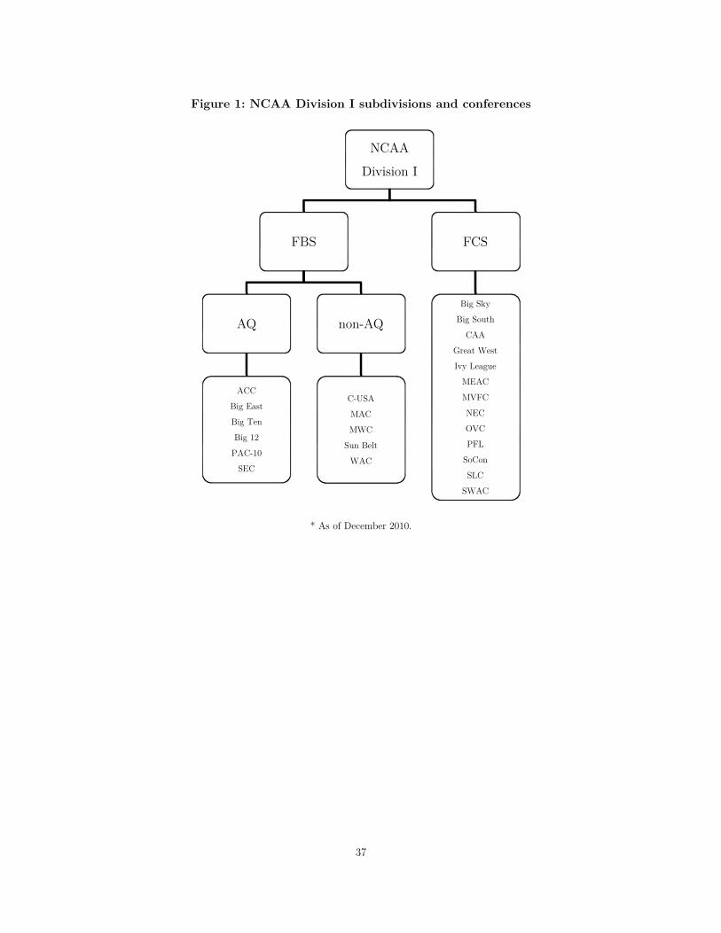
37

Figure 1: NCAA Division I subdivisions and conferences

* As of December 2010.

NCAA

Division I

FBS

AQ

ACC

Big East

Big Ten

Big 12

PAC-10

SEC

non-AQ

C-USA

MAC

MWC

Sun Belt

WAC

FCS

Big Sky

Big South

CAA

Great West

Ivy League

MEAC

MVFC

NEC

OVC

PFL

SoCon

SLC

SWAC

38

Figure 2: Trends for high school graduates and applications

2,300

2,400

2,500

2,600

2,700

2,800

2,900

3,000

3,100

2001 2002 2003 2004 2005 2006 2007 2008 2009

a. High school graduates (K)

2,000

2,500

3,000

3,500

4,000

4,500

5,000

5,500

6,000

2001 2002 2003 2004 2005 2006 2007 2008 2009

b. Applications - total (K)

1.00 1.10 1.20 1.30 1.40 1.50 1.60 1.70 1.80 1.90

2001 2002 2003 2004 2005 2006 2007 2008 2009

c. Applications/student

39

Figure 3: Applications, select schools

6,000

8,000

10,000

12,000

14,000

16,000

18,000

20,000

2001 2002 2003 2004 2005 2006 2007 2008 2009

a. Alabama & Auburn

Alabama Auburn

8,000

10,000

12,000

14,000

16,000

2001 2002 2003 2004 2005 2006 2007 2008 2009

b. Notre Dame

Notre Dame

15,000

20,000

25,000

30,000

35,000

40,000

45,000

2001 2002 2003 2004 2005 2006 2007 2008 2009

c. Texas & Penn St.

Penn St. Texas

8000

10000

12000

14000

16000

18000

2001 2002 2003 2004 2005 2006 2007 2008 2009

d. Oregon & West Virginia

Oregon West Virginia

4,000

6,000

8,000

10,000

12,000

14,000

2001 2002 2003 2004 2005 2006 2007 2008 2009

e. TCU

TCU

40

Figure 4: Applications and changes in the number of wins

Figure 5: Distribution of SAT scores (mass)

-.1

0.1

.2In

cre

ase

in n

orm

aliz

ed a

ppl

ica

tion

s

-7 -6 -5 -4 -3 -2 -1 0 1 2 3 4 5 6 7 8Change in the number of wins

kernel = epanechnikov, degree = 0, bandwidth = 1.34, pwidth = 2.01

0 200 400 600 800 1000 1200 1400 1600

SAT score

Application Admission

41

Figure 6: Segmentation based on SAT scores

400 500 600 700 800 900 1,000 1,100 1,200 1,300 1,400 1,500 1,600

Distribution of SAT Scores

Seg 1 Seg 2 Seg 3 Seg 4 Seg 5