The Distributional Effects of a Carbon Tax on Current

and Future Generations

Stephie Fried∗, Kevin Novan†, William B. Peterman‡

February 1, 2018

Abstract

This paper uses a life cycle model to compare how different approaches for recyclingcarbon tax revenue affect the welfare of agents born in the future steady state versusagents alive when the policy is adopted. Our results demonstrate that the welfareconsequences of a given policy vary substantially across these two groups. For agentsborn into the future steady state, the expected non-environmental welfare costs areminimized when carbon tax revenue is used to reduce an existing distortionary tax. Incontrast, among the agents alive when the policy is adopted, recycling revenue throughuniform, lump-sum rebates results in the largest welfare increase across the policies weexamine. Moreover, we find that the regressivity or progressivity of a policy also differswithin the living population versus the future steady state population. Overall, ourresults illustrate that estimates of the non-environmental welfare costs of carbon taxpolicies that are based on the long-run outcomes miss-represent the near-term conse-quences. Given the potential importance of these near-term effects on the politicalfeasibility of a policy, our findings indicate that, when designing a carbon tax, policymakers must pay careful attention to not only the long-run outcomes, but also to thetransitional welfare effects of the policy.

Keywords: Carbon taxation; overlapping generationsJEL codes: E62; H21; H23

∗Arizona State University, W.P. Carey School of Business. Email: sdfried@asu.edu†University of California, Davis, Department of Agricultural and Resource Economics. Email: kno-

van@ucdavis.edu‡Federal Reserve Board of Governors. Email: william.b.peterman@frb.gov. Views expressed in this paper

are those of the authors’ and do not reflect the views of the Federal Reserve System or its staff.For helpful feedback and suggestions, we thank seminar participants at the Econometric Society North

American Summer meetings (2016), AERE Summer Conference (2016), QSPS (2016), the University of Con-necticut, the Federal Reserve Board of Governors, and the University of California San Diego. Additionally,we thank four anonymous referees for their many suggestions.

1

1 Introduction

Establishing a price on carbon, using either a carbon tax or a cap-and-trade program, is

well understood to be the most efficient approach for reducing greenhouse gas emissions

(Pigou (1920), Dales (1968), Montgomery (1972), Baumol and Oates (1988)). Importantly,

establishing a carbon price could also generate a substantial stream of government revenue.1

This raises an obvious question – how should this revenue be used?

Often, policymakers propose recycling carbon tax revenue in a way that differs from the

approach advocated by the economic literature. For example, one prominent proposal for a

carbon tax was put forth by the Climate Leadership Council (CLC).2 The proposal calls for

the U.S. federal government to impose a carbon tax with all revenue returned to individuals

through uniform, lump-sum payments. In contrast, the economic literature suggests that

it would be far more efficient to use the revenue to reduce pre-existing distortionary taxes

(e.g., taxes on labor or capital income) – a result referred to as the ‘weak double-dividend

hypothesis’ (Goulder (1995), de Mooij and Bovenberg (1998), Bovenberg (1999)).3 It is

important to note, however, that the double-dividend studies largely focus on the long-run

welfare consequences of revenue-neutral carbon tax policies. In this paper, we examine how

different approaches for recycling carbon tax revenues affect the welfare not only of agents

born into the future steady state, but also agents alive at the time the policy is adopted.

Our results reveal that a given policy can have dramatically different impacts on the current

living population compared to agents born in the future steady state.

To examine the welfare impacts of revenue-neutral carbon tax policies, we follow the

macro public finance literature (e.g., Castaneda et al. (2003), Conesa and Krueger (2006),

1A report from the U.S. Department of the Treasury (Horowitz et al. (2017)) estimates that a carbon taxstarting at $49 per ton of CO2 in 2019, and rising to $70 by 2028, would generate $2.2 trillion over ten years.Similarly, estimates from the U.S. Congressional Budget Office suggest that setting a modest CO2 price of$20/ton would raise $1.2 trillion in revenue during the first decade the policy is in place (CBO (2011)).

2The CLC was initially started by a group including former secretaries of state, James A. Baker III andGeorge P. Shultz; former chairmen of the Council of Economic Advisors, Martin Feldstein and GregoryMankiw, and former treasury secretary Henry Paulson Jr.

3Previous studies also highlight that the revenue recycling method can substantially alter the distributionof the welfare changes across income groups (Fullerton and Heutal (2007), Dinan and Rogers (2002), Metcalf(2007), Parry (2004), Parry and Williams (2010)).

2

Conesa et al. (2009), Peterman (2013)) and construct a quantitative, overlapping gener-

ations model (OLG) which incorporates idiosyncratic productivity shocks, mortality risk,

retirement, and Social Security. Using the model, we explore the welfare consequences of

imposing a $35 per ton tax on CO2. This value is in line with the central estimate of the

social cost of carbon previously used in cost-benefit analyses performed by the U.S. Govern-

ment.4 The revenue from this tax is used to either (1) offset revenue generated by a tax on

labor income, (2) offset revenue from a tax on capital income, or (3) is returned in the form of

uniform, lump-sum payments. Consistent with the previous work in the double-dividend lit-

erature, we abstract from the welfare consequences of improvements in environmental quality

and instead focus on the welfare effects stemming from non-environmental channels.5

Focusing first on the steady state outcomes, our results echo the findings from the existing

literature. Among agents born into the future steady state, the expected non-environmental

welfare costs of a carbon tax policy are lower when the carbon tax revenue is used to reduce

either existing distortionary tax. In fact, we find that using the carbon tax revenue to offset

revenue generated by the capital tax leads to an increase in the expected non-environmental

welfare, suggesting that the policy actually reduces the distortions caused by the tax system.

In contrast, recycling the revenue in the form of uniform, lump-sum payments – consistent

with the recent CLC proposal – results in a decrease in the expected non-environmental

welfare of agents born into the future steady steady.

However, our results reveal that revenue-neutral carbon tax policies affect the welfare

of the current living agents very differently than the welfare of agents born into the future

steady state. In particular, we find that using carbon tax revenue to reduce the labor or

capital tax will be far more costly among the living population as opposed to the future

steady state cohorts. In contrast, the lump-sum rebate policy is far less costly for the living

population, actually leading to an increase in average welfare. Interestingly, among the

three policies we consider, the uniform lump-sum rebate results in the largest reduction in

4For example, the IAWG (2013) reports a central carbon cost estimate of $38/ton of CO2 in 2015 dollars.5However, across each of the policy options we simulate, the reduction in energy consumption is very

stable. As a result, the welfare changes driven by environmental quality improvements would likely similaracross the policies we consider.

3

expected steady state welfare but also the largest increase in average welfare among the living

population. Moreover, our results highlight that, not only do the average welfare impacts

vary depending on how the carbon tax revenue is recycled, the regressivity or progressivity

of a given policy also varies with whether we focus on the living population or the future

steady state population.

Throughout our analysis, we highlight two factors that cause the welfare impacts to

differ among the current living agents versus those born into the future steady state. First,

following the adoption of a carbon tax policy, the factor prices do not immediately adjust

to their new, long-run equilibrium levels. Second, unlike agents born into the steady state,

agents alive when the carbon tax is adopted only experience the policy for a portion of their

lifetime. This proves to be important because the impact a carbon tax policy has on an

agent’s remaining lifetime welfare varies substantially with the agent’s age.

The present paper builds on several studies examining the transitional welfare impacts of

carbon tax policies. Leach (2009) combines an OLG model with a climate model to explore

how the environmental and non-environmental welfare impacts of a carbon tax policy differ

across generations. Similarly, Rausch (2013) and Carbone et al. (2013) examine the non-

environmental welfare impacts of alternative revenue-neutral carbon tax policies using life

cycle models.6 All three of these previous studies examine models with a single representative

agent for each age cohort. In contrast, our life cycle model incorporates within age cohort

income heterogeneity through individual-specific productivity fixed effects as well as through

idiosyncratic productivity shocks.7 The inclusion of within cohort heterogeneity enables us

to directly examine the general equilibrium welfare impacts across both age and income

groups.8 Thus, our welfare measure incorporates the policy’s impacts not only on efficiency,

but also on equity. In addition, by modeling households’ utility using a non-homothetic

6Rausch (2013) also consider the impacts of using carbon revenues to reduce the size of the federal debt.7Chiroleu-Assouline and Fodha (2014) also include within-cohort heterogeneity in a life cycle model

through the use of ability fixed effects. However, the authors focus solely on the welfare effects of recyclingthe revenues from a carbon tax through a labor tax rebate in the long run steady state.

8In a related analysis, Williams et al. (2015) predict distributional impacts using the estimates fromCarbone et al. as inputs in a partial equilibrium, microsimulation model. The model translates the predictedincome changes into estimates of the welfare impacts across income groups during the initial year the policyis in place – not over the agents’ lifetimes.

4

utility function, we are able to incorporate the fact that low income households use a higher

share of their expenditures on energy, making the carbon tax by itself regressive.

To be clear, the objective of our analysis is not to exhaustively evaluate the full range

of revenue-neutral carbon tax policy options available to policymakers. Instead, our goal

is to illustrate an important point. Specifically, the welfare and distributional impacts of

revenue-neutral carbon tax policies can differ dramatically across agents living during the

transition and those born into the future, long-run steady state.9 Given that the current

living agents – not agents born into a future steady state – are ultimately responsible for

implementing a carbon tax, it is particularly important to understand the near-term welfare

impacts of alternative policies in order to design a politically feasible option. Our findings

suggest that it is more beneficial to the living population to return carbon tax revenue

through uniform, lump-sum rebates instead of through reductions in distortionary taxes,

and thus, the lump-sum rebate approach may in fact be the easier policy to implement.

The remainder of the paper proceeds as follows. Section 2 introduces the OLG model.

Section 3 discusses the functional forms in the model and the calibration of the key pa-

rameters. Section 4 compares the aggregate welfare and distributional impacts under the

alternative carbon tax policies in the long-run steady state and within the current living

population. Section 5 concludes.

2 Model

2.1 Demographics

Agents enter the model when they start working, which we approximate with a real world age

of 20, and can live to a maximum age of J . Thus, there are J − 19 overlapping generations.

A continuum of new agents is born each period and the relative size of the newborn cohort

grows at a constant rate, n. Lifetime length is uncertain and mortality risk varies over the

9Previous studies in the macroeconomic and public finance literatures highlight that, across a varietyof settings, the steady state and transition welfare effects of tax policies can differ substantially (e.g., seeDomeij and Heathcote (2004), Fehr and Kindermann (2015), Dyrda et al. (2015)).

5

lifetime. Parameter Ψj denotes the probability an agent lives to age j+1 conditional on being

alive at age j. All agents who live to age J die with probability one the following period,

i.e. ΨJ = 0. Since agents are not certain how long they will live, they may die with positive

asset holdings. In this case, we treat the assets as accidental bequests and redistribute them

lump-sum across all living individuals during period t in the form of transfers T at . All agents

are forced to retire at the exogenously determined age jr.

2.2 Households

An individual is endowed with one unit of productive time per period that can be divided

between labor and leisure. In period t, at age j, agent i earns labor income yhi,j,t ≡ wt ·

µi,j,t · hi,j,t, where wt is the market wage-rate during period t, hi,j,t denotes hours worked,

and µi,j,t is the agent’s idiosyncratic productivity. Following Kaplan (2012), the log of an

agent’s idiosyncratic productivity consists of four additively separable components,

log µi,j,t = εj + ξi + νi,j,t + θi,j,t. (1)

Component εj governs age-specific human capital and evolves over the life cycle in a predeter-

mined manner. Component ξi ∼ NID(0, σ2ξ ) is an individual-specific fixed effect (i.e. ability)

that is observed when an agent enters the model and is constant for an agent over the life

cycle. Component θi,j,t ∼ NID(0, σ2θ) is an idiosyncratic transitory shock to productivity

received every period, and νi,j,t is an idiosyncratic persistent shock to productivity, which

follows a first-order autoregressive process:

νi,j,t = ρνi,j−1,t−1 + ψi,j,t with ψi,j,t ∼ NID(0, σ2ν) and νi,20,t = 0. (2)

Thus, the average labor productivity of agents differs across cohorts along one dimension,

their age-specific human capital, εj. Agents within an age cohort are differentiated along

three dimensions that affect their labor productivity: their ability, ξi, their current transitory

shock, θi,j,t, and their current persistent shock, νi,j,t. Different ability types, and the initial

6

realization of the i.i.d. shock, θi,j,t, generate an initial productivity distribution within the

cohort of 20 year old entrants to the model. Different realizations of the persistent shock

νi,j,t over the lifetime cause the within cohort variation to grow with age.

We assume that agents cannot insure against idiosyncratic productivity shocks by trading

explicit insurance contracts. Moreover, we assume that there are no annuity markets to insure

against mortality risk. However, agents are able to partially self insure against labor-income

risk by purchasing risk-free assets, ai,j,t, that have a pre-tax rate of return, rt.

Agents split their income between investing in the risk-free asset and consumption. When

considering how a carbon tax would affect individuals’ consumption, it is important to note

that carbon emitting energy sources are not only used in the production of final consumer

goods, but carbon-based energy sources are also consumed directly by individuals as a fi-

nal good (e.g., electricity, gasoline, heating oil, etc.). Therefore, in our model, agents can

consume a generic consumption good, ci,j,t, as well as a carbon emitting energy good, eci,j,t.

As previous studies highlight (Metcalf (2007), Hassett et al. (2009)), the direct impact of

a carbon tax – prior to any revenue recycling – is likely to be regressive. This is due to the

fact that lower income households devote a larger share of their budgets to energy. To ensure

that our model captures this negative relationship between income and energy consumption

shares, we assume that all agents must consume a minimum amount of energy, e, and that

agents derive no utility from the energy consumed up to this subsistence level.10

In each period, an agent chooses labor, savings, generic consumption, and energy con-

sumption, subject to their budget constraint, in order to maximize their expected stream of

future discounted lifetime utility given by

u(ci,j,t, eci,j,t − e, hi,j,t) + E

J∑

k=j+1

βk−jk−1∏q=j

(Ψq)u(ci,k,t+k−j, eci,k,t+k−j − e, hi,k,t+k−j)

. (3)

We take the expectation in equation (3) with respect to the stochastic processes governing the

10Pizer and Sexton (2017) highlight that variation in energy expenditure shares can also arise withinincome groups (e.g., e could vary across urban and rural locations). We abstract from this variation,effectively assuming that spatial heterogeneity in e is uncorrelated with idiosyncratic productivity shocks.

7

idiosyncratic productivity shocks. Agents discount future utility by β, the discount factor.

In addition, they incorporate mortality risk by discounting the next period’s utility by Ψj.

An agent’s utility increases with consumption of either energy or the generic consumption

good and decreases with more hours worked.

2.3 Production

Perfectly competitive firms produce a generic final good, Yt, from capital, Kt, aggregate

labor (measured in efficiency units), Nt, and carbon-emitting energy, Ept , according to the

production function, Yt = f(Kt, Nt, Ept ). The final good is the numeraire and can be used

for, consumption, investment, and to purchase energy at exogenous price pe.

This model of production with an exogenous energy price is consistent with the assump-

tion that the country behaves as a small open economy with respect to energy. The country

imports energy at price pe in exchange for the final good with zero trade balance in every pe-

riod. This of course assumes that the energy price would not respond to changes in demand

caused by the climate policy. In practice, this is likely to be a minor simplification. In our

carbon tax simulations, U.S. energy consumption falls approximately fifteen percent, which

would represent a very small (2.4 percent) change in global energy demand, suggesting that

the resulting general equilibrium effects of unilateral U.S. climate policy on global energy

prices are also likely to be small.11

To provide insight into how a decrease in energy prices – which is driven by the adoption

of a domestic carbon tax – could affect our results, we also analyze a two-sector model

in which all energy is produced domestically from capital and labor and the final good is

produced from capital, labor, and domestic energy, as in Barrage (2016). While assuming

that energy prices are constant will certainly understate the response of energy prices to

a carbon tax, assuming all energy is produced in a domestic energy sector will certainly

11In 2012, U.S. carbon-energy use accounted for approximately 16 percent of global carbon-energy use.We calculate the U.S. fraction of carbon-energy from the ratio of U.S. carbon emissions to global carbonemissions. We use emissions data as opposed to data on energy production and/or consumption becausethe emissions data capture all U.S. carbon-related activities. Data on carbon emissions are from the EIAinternational energy statistics: http://www.eia.gov/.

8

overstate the endogenous response of the energy price to a carbon tax policy. Therefore, our

main model (i.e. assuming a constant world energy price) and our robustness check effectively

bound the potential responses of energy prices to a domestic carbon tax policy. We find that

while there are small quantitative differences, the results do not change qualitatively with

the assumption of a constant versus variable energy price.

2.4 Government Policy

The government performs three activities: (1) it consumes resources in an unproductive

sector, G, (2) it runs a pay-as-you-go Social Security system, and (3) it taxes capital income,

labor income, and energy (i.e. a carbon tax) to finance G. The government pays Social

Security benefits, St, to all agents that are retired. Each agent receives a constant payment

each period, which is independent of the specific agent’s lifetime earnings. The government

finances the Social Security system with a flat tax on labor income, τ st . Half of the payroll

taxes are withheld from labor income by the employer and the other half are paid directly by

the employee. The payroll tax rate is set such that the Social Security system has a balanced

budget in every period.

The government taxes each agent’s capital income, yki,j,t, according to a constant marginal

tax rate, τ k. An agent’s capital income is the return on her assets plus the return on any

assets she receives as accidental bequests, yki,j,t ≡ rt(ai,j,t + T at ). The government taxes labor

income according to a progressive tax schedule, T h(yhi,j,t), where yhi,j,t denotes the agent’s

taxable labor income. A working agent’s taxable labor income is her labor income, yhi,j,t, net

of her employer’s contribution to Social Security which is not taxable under U.S. tax law.

Thus, yhi,j,t ≡ yhi,j,t(1− τ st /2), where (τ st /2)yhi,j,t is the employer’s Social Security contribution.

Consistent with U.S. tax law, for agents whose annual income exceeds a given threshold,

the government also taxes a portion of their Social Security benefits at the labor income tax

rate. The taxes paid on an agent’s Social Security benefits are defined by T s(St, yki,j,t).

Finally, the government can tax carbon energy at a constant rate. This tax not only raises

government revenue, but it can also reduce the use of carbon based energy. The carbon tax,

9

τ c, is designed to place a price on the externality, carbon. Thus, the government applies the

tax per unit of energy consumed, raising the price of energy from pe to pe + τ c.12 In one of

the tax policies, the government rebates this carbon-tax revenue through uniform lump-sum

transfers to the households, T ct .

2.5 Definition of a Stationary Competitive Equilibrium

In this section, we define a stationary competitive equilibrium. In the long-run steady state,

the factor prices, tax parameters, and aggregate macroeconomic variables will be constant.

The individual state variables, x, are asset holdings, a, idiosyncratic labor productivity, µ,

and age j. In addition, we signify an agent’s chosen level of capital savings in the subsequent

period as a′. We suppress the i, j, and t subscripts throughout the stationary equilibrium

definition. The summations are taken over the distribution of agents over the state space, x.

Given Social Security benefits, S, government expenditures, G, demographic parameters,

n,Ψj, a sequence of age-specific human capital, εjjr−1j=20, a labor-tax function, T h : R+ →

R+, a capital-tax rate, τ k, a carbon-tax rate, τ c, transfers from the climate policy, T c, an

energy price, pe, a utility function U : R+ × R+ × R+ → R+, factor prices, w, r, pe, and

capital depreciation rate δ, a stationary competitive equilibrium consists of agents’ decisions

rules, c, h, ec, a′, firms’ production plans, Ep, K,N, transfers from accidental bequests

T a, a social security tax rate, τ s, and the distribution of individuals, Φ(x), such that the

following holds:

1. Given prices, policies, transfers, benefits, and ν that follows equation (2) the agent

maximizes equation (3) subject to:

c+ (pe + τ c)ec + a′ =

µhw(1− τ s) + (1 + r(1− τ k))(a+ T a)− T h(µhw(1− .5τ s)

)+ T c for j < jr

(4)

12Given that fossil fuel combustion accounts for over 80 percent of GHG emissions, a carbon tax behavesmuch like a tax on energy. This of course abstracts from substitution between fossil fuel energy sources withvarying carbon intensities that could occur with a carbon tax.

10

c+ (pe + τ c)ec + a′ = S − T s(S, yk) + (1 + r(1− τ k))(a+ T a) + T c for j ≥ jr

c ≥ 0, ec ≥ 0, 0 ≤ h ≤ 1, a ≥ 0, a20 = 0

2. Firms’ demands for K, N , and Ep satisfy:

r =∂f(K,N,Ep)

∂K− δ (5)

w =∂f(K,N,Ep)

∂N(6)

pe + τ c =∂f(K,N,Ep)

∂Ep(7)

3. The Social Security tax satisfies:

τ s =S∑

j≥jr Φ(x)

wN(8)

4. Transfers from accidental bequests satisfy:

T a =∑

(1−Ψ)a′Φ(x) (9)

5. The government budget balances:

G =∑[

τ kr(a+ T a) + T h(µhw(1− .5τ s)

)+ T s(S, yk) + τ cec

]Φ(x) + τ cEp − T c

(10)

11

6. Markets clear:

K =∑

aΦ(x), N =∑

µhΦ(x) (11)

∑(c+ peec + a′)Φ(x) +G+ peEp = Y + (1− δ)K (12)

7. The distribution of Φ(x) is stationary. That is, the law of motion for the distribution

of individuals over the state space satisfies Φ(x) = QΦΦ(x) where QΦ is the one-period

recursive operator on the distribution.

3 Calibration and Functional Forms

We calibrate the model in two steps. In the first step, we choose parameter values for

which there are direct estimates in the data. In the second step, we calibrate the remaining

parameters so that certain targets in the model match the values observed in the U.S.

economy. Table 1 reports the parameter values.

3.1 Demographics

Agents enter the model at age 20 and are exogenously forced to retire at age jr = 66. If an

individual survives until 100, she dies the next period. We choose the conditional survival

probabilities based on the estimates in Bell and Miller (2002). We adjust the size of each

cohort’s share of the population to be consistent with a population growth rate of 1.1 percent.

3.2 Idiosyncratic and Age-Specific Productivity

We calibrate the labor productivity shocks based on the estimates from Appendix E of

Kaplan (2012). These parameters governing the permanent, persistent, and transitory id-

iosyncratic shocks to individuals’ productivity are set such that the shocks are distributed

12

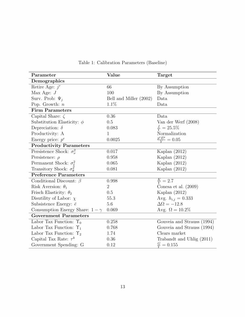
Table 1: Calibration Parameters (Baseline)

Parameter Value TargetDemographicsRetire Age: jr 66 By AssumptionMax Age: J 100 By AssumptionSurv. Prob: Ψj Bell and Miller (2002) DataPop. Growth: n 1.1% DataFirm ParametersCapital Share: ζ 0.36 DataSubstitution Elasticity: φ 0.5 Van der Werf (2008)Depreciation: δ 0.083 I

Y= 25.5%

Productivity: A 1 Normalization

Energy price: pe 0.0025 peEp

Y= 0.05

Productivity ParametersPersistence Shock: σ2

ν 0.017 Kaplan (2012)Persistence: ρ 0.958 Kaplan (2012)Permanent Shock: σ2

ξ 0.065 Kaplan (2012)Transitory Shock: σ2

θ 0.081 Kaplan (2012)Preference ParametersConditional Discount: β 0.998 K

Y= 2.7

Risk Aversion: θ1 2 Conesa et al. (2009)Frisch Elasticity: θ2 0.5 Kaplan (2012)Disutility of Labor: χ 55.3 Avg. hi,j = 0.333Subsistence Energy: e 5.6 ∆Ω = −12.8Consumption Energy Share: 1− γ 0.069 Avg. Ω = 10.2%Government ParametersLabor Tax Function: Υ0 0.258 Gouveia and Strauss (1994)Labor Tax Function: Υ1 0.768 Gouveia and Strauss (1994)Labor Tax Function: Υ2 1.74 Clears marketCapital Tax Rate: τ k 0.36 Trabandt and Uhlig (2011)Government Spending: G 0.12 G

Y= 0.155

13

log normally with a mean of one. In particular, the shock parameters are set at ρ = 0.958,

σ2ξ = 0.065, σ2

ν = 0.017 and σ2θ = 0.081. To solve the model, we discretize the shocks using

two states to represent the transitory and permanent shocks and five states for the persistent

shock.13 We set εjjr−1j=20 to match the average hourly earnings estimated in Kaplan (2012).

3.3 Preferences

Agents have time-separable preferences over a consumption-energy composite, ci,j,t, and

hours, hi,j,t. The utility function is given by

U(ci,j,t, hi,j,t) =c1−θ1i,j,t

1− θ1

− χh

1+ 1θ2

i,j,t

1 + 1θ2

(13)

where ci,j,t = cγi,j,t(eci,j,t − e)1−γ. This functional form is separable and homothetic in the

consumption-energy composite and labor, implying a constant Frisch elasticity of labor sup-

ply regardless of hours worked. We determine β to match the U.S. capital-output ratio of

2.7. We choose χ such that agents spend an average of one third of their time endowment

working. Following Conesa et al. (2009), we set the coefficient of relative risk aversion (θ1)

equal to 2 and consistent with Kaplan (2012), we set the Frisch elasticity (θ2) equal to 0.5.14

Previous work notes that the carbon tax by itself may be regressive because lower income

individuals devote a larger share of their total consumption expenditures to energy (Metcalf

(2007), Hassett et al. (2009)). Figure 1 plots the average energy budget share for each ex-

penditure decile using data from the Consumer Expenditures Survey (CEX) from 1981-2003.

Consistent with these previous findings, the average energy budget share falls considerably

as average expenditures rise. At the extremes, energy expenditures are over 15 percent of

total expenditures for the lowest decile but just over six percent for the highest decile.

13We use the Rouwenhorst method to discretize the persistent shock. This method is well-suited fordiscretizing highly persistent shocks with a small number of states (Kopecky and Suen (2010)).

14Peterman (2016) demonstrates that setting the Frisch elasticity at 0.5 is consistent with including hoursfluctuations on the intensive margin only.

14

Figure 1: Energy Budget Share: CEX

2 4 6 8 10

Expenditure Decile

6

8

10

12

14

16

Per

cent

Note: Figure displays average energy budget shares by expenditure decile from the 1981-2003 Consumer Ex-penditures Survey. Energy expenditures include household expenditures on electricity, natural gas, gasoline,and coal and oil in the home. We determine the average energy budget share for each decile conditional onthe household’s age. Specifically, we first calculate the average energy budget share for each decile withineach age bin. Second, for each decile, we calculate a population weighted average across the age bins wherethe weights are determined by the share of the population in each bin.

Together, the utility parameters e and γ determine a household’s energy share of total

consumption and how this share varies with the household’s total consumption expenditures.

In particular, the energy share of total consumption expenditures, Ωt, is

Ωt = (1− γ) +γpee

(1− γ)(ci,j,t + peeci,j,t). (14)

If e = 0, energy’s share of total expenditure equals 1− γ regardless of the level of an agent’s

total expenditure. However, if e > 0, energy’s share will decrease with total expenditure.

Moreover, higher e increases the responsiveness of energy share to changes in total expen-

diture. We set e and γ such that our model matches the data with respect to the average

energy share in the population and the percent difference in the energy share of the top

and bottom halves of the expenditure distribution (∆Ωt =Ωtopt −Ωbottomt

Ωbottomt× 100). The average

energy share in the population is 10.2 percent. Moreover, we target ∆Ωt = −12.8 percent.15

15The actual differential measured in the CEX is 33 percent (∆Ω = −33 percent). However, this targetneeds to be adjusted because the overall differential in total expenditures between the top and bottom halvesof the distribution is larger in the data than in our model. In particular, it is 142 percent in the data and

15

Table 2 reports the value of the moments we target in the model and their corresponding

value in the data. Overall, the model fits these targets quite closely.

Table 2: Model FitMoment Target ModelEnergy share: Ω 0.102 0.102Energy share difference: ∆Ω -0.128 -0.128Hours: H 0.333 0.333Govt spending to output: G

Y0.155 0.155

Capital to output: KY

2.7 2.700

3.4 Production

The production technology features a constant elasticity of substitution, φ, between a capital-

labor composite, KζtN

1−ζt , and energy,

Yt = A

[(KζtN

1−ζt

)φ−1φ

+ (Ept )

φ−1φ

] φφ−1

. (15)

We use 0.5 for the elasticity of substitution between the capital-labor composite and energy,

φ. This parameter choice is within the range of estimates reported in Van der Werf (2008).

We use ζ = 0.36 for capital’s share in the capital-labor composite. We calibrate the price of

energy, pe, so that energy’s share of production is five percent.

3.5 Government Policies and Tax Functions

We begin our policy experiments in a baseline equilibrium that mimics the U.S. tax code.

We follow the quantitative public finance literature and use estimates of the U.S. tax code

from Gouveia and Strauss (1994). Gouveia and Strauss (1994) match the U.S. income tax

only 54 percent in our model. The key reason for the smaller differential in total expenditures in our model isthat the productivity shocks are assumed to be log normal. This distributional assumption, while standardin the literature, results in our model failing to capture the extreme top tail of the income distribution.Therefore, we adjust for the smaller expenditure variance in our model and target ∆Ω = −12.8 percent. Inparticular, we adjust ∆Ω so that 54

142 = −12.8−33 .

16

code to the data using a three parameter functional form:

T h(yhi,j,t; Υ0,Υ1,Υ2) = Υ0

(yhi,j,t −

((yhi,j,t)

−Υ1 + Υ2

)−1Υ1

). (16)

Parameter Υ0 governs the average tax rate and parameter Υ1 controls the progressivity of

the tax policy. To ensure that taxes satisfy the budget constraint, we leave parameter Υ2

free in the baseline. Gouveia and Strauss (1994) estimate that Υ0 = 0.258 and Υ1 = 0.768.

A portion of Social Security benefits are taxable at the labor income tax rate for high

income, retired agents. Consistent with U.S. tax law, 85 percent of a retiree’s Social Security

payments are included as taxable labor income if the retiree’s income exceeds 76 percent of

average labor income and 50 percent of the benefits are included if the retiree’s income is

between 76 percent and 56 percent of the average labor income. None of the Social Security

benefits are included as taxable labor income if the agent’s income is below the 56 percent

threshold. The incomes for most retirees are below this 56 percent threshold.16

We determine government consumption, G, so that it equals 15.5 percent of output, the

average value in the U.S data.17 We set the tax rate on capital income, τ k, to 36 percent

based on estimates in Kaplan (2012), Nakajima (2010) and Trabandt and Uhlig (2011). To

determine the size of the Social Security payments in the baseline steady state, we follow

Conesa and Krueger (2006) and assume that retired agents receive 50 percent of the average

income of all working individuals

S = 0.5

(wN∑

j<jr Φ(x)

). (17)

16U.S. tax law states that 85 percent of Social Security income is taxable for single households withtotal income above 34,000 in 2014 dollars and 50 percent is taxable for single households with total in-come above 25,000 in 2014 dollars. We translate these to thresholds based on the percentage of laborincome using data on estimated average earnings in the Annual Statical Supplement from the Social Secu-rity Administration (https://www.ssa.gov/policy/docs/statcomps/supplement/2015/highlights.html). Seehttps://www.ssa.gov/planners/taxes.html for a details on U.S. tax law regarding Social Security benefits.

17To calculate the empirical value of GY , we use total government expenditures net of Social Security

payments because Social Security is financed by a separate payroll tax in our model. Data on governmentexpenditures, social security benefits and GDP are from the BEA. We use the average value of G

Y from1998-2007. Additionally, since we assume a small open economy with respect to energy, the model value ofGDP (the denominator of G

Y ) equals the value of total production minus the value of energy imports.

17

Each period, retirees receive this constant Social Security payment, which is denominated

in terms of the numeraire. However, in the simulations, the carbon tax raises the price of

the energy-good which reduces the relative price of the numeraire, and thus, decreases the

purchasing power of the Social Security payments. In practice, the U.S. government adjusts

Social Security payments each year to ensure that the purchasing power remains constant.

Consistent with this policy, we adjust the Social Security payment in each simulation to

ensure that the retiree can buy the same bundle of energy and non-energy goods as she

could in the baseline steady state.18 We choose the payroll tax, τ st , to ensure that the Social

Security system has a balanced budget in every period.

Finally, in the computational experiment, we analyze a carbon tax set at $35 dollars per

ton of CO2. To calibrate the size of the tax in the model, we calculate the empirical value of

the tax as a fraction of the price of a fossil energy composite of coal, oil, and natural gas in

2011. We calculate the price of this energy composite averaging over the price of each type

of energy in 2011, and weighting by the relative consumption. Similarly, we calculate the

carbon emitted from the energy composite by averaging over the carbon intensity of each

type of energy in 2011, and weighting by the relative consumption. This process implies that

a $35 per ton carbon tax equals 32 percent of our composite fossil energy price.

4 Results

4.1 Computational Experiment

To examine the welfare consequences of a carbon tax, we simulate a baseline economy with no

carbon tax and conduct a series of counterfactual simulations in which we impose a constant

carbon tax set at $35 per ton of CO2.19 We simulate three different policies which vary in

how the government rebates the revenue generated from the carbon tax: (1) rebates through

18Specifically, Social Security payments in each simulation equal Social Security payments in the baseline

times ce(pe+τc)cepe+c where ce and c are the baseline values of energy and non-energy consumption, respectively.

19To solve for the competitive equilibrium in the baseline and under each tax policy, we use an algorithmbased on Heer and Maussner (2009). For details on the solution algorithms, see Appendix A.

18

equal, lump-sum transfers to households, (2) rebates through a reduction in the capital tax

rate, and (3) rebates through a reduction in the labor tax rate. To isolate the effect of

the carbon tax by itself, we also analyze a fourth case, the no-rebate case, in which the

government uses the carbon tax revenue in a non-productive sector (i.e. “throws it into the

ocean”).20 Consistent with much of the double-dividend literature, we specifically examine

the non-environmental welfare consequences of the carbon tax policies.21

4.2 Aggregate welfare effects

Recall, our objective is to examine how the carbon tax policies affect not only the welfare of

agents born into the future steady state, but also the welfare of agents alive at the time the

carbon tax is adopted. To measure the aggregate welfare impacts, we use the consumption

equivalent variation (CEV). In the steady state, the CEV measures the uniform percentage

change in an agent’s expected consumption that is required to make her indifferent – prior to

observing her idiosyncratic ability, productivity, and mortality shocks – between the baseline

steady state and the steady state under the carbon tax policy.

In contrast, for cohorts alive when the policy is adopted, the CEV captures the effect

of the policy over their remaining lifetimes, and thus, varies based on the cohort’s age at

the time the policy is adopted. Specifically, to calculate the CEV of the policy for a given

age cohort, we compute the uniform percent change in consumption across all agents in the

cohort that would be necessary, in every remaining period of their lifetimes, so that the

cohort’s average expected utility is the same as if they were to live the rest of their lives in

the baseline steady state. The aggregate CEV among the living population is the weighted

average of the CEVs for each living age cohort. Each cohort’s weight is the share of the

20Under the different policies, the carbon tax leads to changes in aggregate labor and capital, whichaffect aggregate tax-revenue from the non-energy tax sources. Thus, in addition to rebating the carbon taxrevenue, we adjust the Social Security tax to balance the Social Security budget and we adjust the averagelabor tax rate to ensure the government budget constraint holds. The progressivity parameters of the labortax function, Υ1 and Υ2, are held constant at their baseline values. Tables 7 and 8 in Appendix B reportthe tax parameters and the revenue raised from each of the tax instruments in the baseline steady state andin each of the four simulations.

21Our results reveal that the reduction in energy use, and therefore, the welfare impacts caused by envi-ronmental quality changes, are very similar across the different rebate options. See Appendix C.

19

expected net present value of the remaining consumption for that cohort relative to the total

remaining lifetime consumption for all living cohorts.22 Therefore, the weights account for

the fact that the resources required to fund a one percent increase in a younger cohort’s

remaining lifetime consumption exceed the resources needed to fund a one percent increase

in an older cohort’s remaining lifetime consumption.

Table 3 reports the aggregate CEV for agents born into the future steady state and

for the living population. A negative CEV indicates that the expected non-environmental

welfare is reduced by the carbon tax policy while a positive CEV indicates that the expected

non-environmental welfare increases. First, notice that, in the future steady state, the non-

environmental welfare costs of the carbon tax policy are lower when the revenue is used

to offset a pre-existing distortionay tax, not when the revenue is returned in the form of

uniform, lump-sum rebates. Specifically, the CEV under the lump-sum rebate is -1.26 percent

compared to only -0.33 percent under the labor tax rebate and 0.29 percent under the capital

tax rebate. This pattern is consistent with the weak double-dividend literature.

Table 3: Aggregate Welfare Effects (CEV, percent)

No Lump-sum Capital LaborRebate Rebate Rebate Rebate

Steady State -6.47 -1.26 0.29 -0.33Living Population -4.65 0.26 0.06 -0.63

In contrast, for the living population, the pattern is quite different. We find that using

carbon tax revenue to reduce the labor or capital tax will be more costly for those alive at

the time a carbon tax is implemented. If labor tax revenue is offset, the non-environmental

welfare of a living agent will fall, on average, by the equivalent of 0.63 percent of expected

future lifetime consumption. This drop in welfare is twice as large as the expected welfare

decrease experienced by agents born into the future steady state. Similarly, if capital tax

revenue is offset, agents alive at the time of adoption will experience an average welfare

increase of only 0.06 percent of expected future lifetime consumption – one fifth as large

22We calculate the cohort weights in the steady state.

20

as the expected welfare increase experienced by agents born into the steady state. In con-

trast, the lump-sum rebate policy leads to an increase in average welfare among the living

population equal to 0.26 percent of expected future lifetime consumption. In the end, the

results summarized in Table 3 reveal that, while a policy consistent with the recent Climate

Leadership Council proposal – i.e. a carbon tax combined with a uniform lump-sum rebate

– will impose relatively large non-environmental welfare costs on agents in the long-run, it

may ultimately be the preferred policy among the living population.

To understand why the welfare impacts differ for the living population versus agents

born in the future steady state, recall that the long-run impacts reflect the change in a

newborn agent’s expected lifetime welfare. In contrast, the welfare effect for the living

population reflects the average impact over the remainder of the living cohorts’ lifetimes.

These measures differ largely because the welfare impacts vary over agents’ life cycles.23 For

example, if a policy is relatively less costly for older cohorts, then the policy will impose

smaller average costs on the living agents compared to those born in the future steady state.

Figure 2: Transition Dynamics: Percent Change From the Baseline

0 20 40 60 80 100

Year

-10

0

10

20

30

40

Per

cent

Chan

ge

After-Tax Risk-Free Rate

No Rebate

Lump-sum

Capital

Labor

0 20 40 60 80 100

Year

-6

-4

-2

0

2

4

Per

cent

Chan

ge

Approximate After-Tax Wage

Note: The figures plot the percentage changes in the after-tax returns to capital and labor relative to thebaseline steady state values after the policy is adopted. Year zero is the first year under the policy.

To illustrate why the welfare effects vary over the life cycle, Figure 2 first highlights

23In addition, the effects can vary for newborn agents when the policy is adopted versus agents born inthe long-run steady state because the factor prices take time to adjust to their new steady state values.

21

how the after-tax wage and risk-free rate adjust following the adoption of a tax policy.24

Ultimately, the welfare consequences of these price changes depend critically on the relative

importance of income from capital and labor, which in turn, depend on an agent’s age.

Figure 3 plots the share of remaining lifetime income from different sources for each age

cohort. Intuitively, labor’s share of remaining income falls as cohorts age and have fewer

working years left. The share of remaining income from capital rises throughout working life

as agents accumulate savings and falls as agents deplete their savings during retirement.25

24Appendix C.2 discusses these factor price movements in more detail.25Similarly, Social Security income’s share rises with age. The remaining lifetime income from transfers

is relatively stable over the life cycle. Mechanically it rises slightly during the end of life, as the increasedmortality risk drives down the remaining lifetime income.

22

Figure 3: Share of Remaining Lifetime Income by Source

20 40 60 80 100

Age

0

20

40

60

80

100

Per

cent

Remaining Lifetime Labor Income

Relative to Remaining Lifetime Income

20 40 60 80 100

Age

0

20

40

60

80

100

Per

cent

Remaining Lifetime Capital Income

Relative to Remaining Lifetime Income

20 40 60 80 100

Age

0

20

40

60

80

100

Per

cent

Remaining Lifetime Lump-Sum Transfer

Relative to Remaining Lifetime Income

20 40 60 80 100

Age

0

20

40

60

80

100

Per

cent

Remaining Lifetime Social Security Payments

Relative to Remaining Lifetime Income

Note: The figure shows the average share of remaining lifetime income from various sources for each agecohort. The figure displays the average share of remaining lifetime income from labor income under thelabor-tax rebate policy, from capital income under the capital-tax rebate policy, and from lump-sum reim-bursements of carbon tax payments under the lump-sum rebate policy, and from Social Security paymentsin the baseline. The only source of lifetime income that is not pictured is accidental bequests.

The movements in factor prices, combined with the age-dependent shares of remaining

lifetime capital, labor, and transfer income, cause the welfare consequences of a carbon tax

policy to vary considerably with the cohort’s age when the government introduces the policy.

To highlight this variation over the life cycle, Figure 4 plots the average non-environmental

welfare effects conditional on the agent’s age at the time a carbon tax policy is adopted.

The top right panel of Figure 4 illustrates that the lump-sum rebate imposes slight costs

on young cohorts while providing substantial gains for the older living cohorts. These older

23

agents receive little to no remaining income from labor, and therefore, do not suffer from the

decline in the after-tax wage (see Figure 2). While the older agents are harmed slightly by

the small initial decline in the after-tax risk free rate (see Figure 2), this effect is dominated

by the welfare gains from the lump-sum transfer. Aggregating across the living cohorts, the

lump-sum rebate policy ultimately leads to a sizable increase in expected welfare.

Figure 4: CEV: Agents Alive At Time of Shock

20 40 60 80 100

Age at Time of Adpotion

-10

-5

0

5

10

Per

cent

No Rebate

20 40 60 80 100

Age at Time of Adpotion

-10

-5

0

5

10

Per

cent

Lump-Sum Rebate

20 40 60 80 100

Age at Time of Adpotion

-10

-5

0

5

10

Per

cent

Captial-Tax Rebate

20 40 60 80 100

Age at Time of Adpotion

-10

-5

0

5

10

Per

cent

Labor-Tax Rebate

Note: The figure displays the average non-environmental welfare effects of each carbon tax policy for eachage cohort at the time the policy is adopted. The welfare impacts are measured as the uniform percentchange in expected future consumption in each period needed to make the average welfare for a given cohortthe same as in the baseline (i.e., no carbon tax) case. Positive numbers represent a welfare increase as aresult of the tax policy change and negative numbers represent a welfare decrease.

Recall, rebating revenue in the form of a reduction in the capital tax leads to an immediate

increase in the after-tax risk-free rate and an immediate reduction in the after-tax wage. The

24

bottom left panel of Figure 4 reveals that the large increase in the after-tax risk-free rate

increases the non-environmental welfare of agents close to retirement age, the point in the

life cycle when capital income accounts for the greatest share of remaining lifetime income

(see Figure 3). Among the youngest agents, the benefits from the increase in the after-tax

risk-free rate are outweighed by the costs incurred by the reduction in the after-tax wage.

Aggregating across all of the living cohorts, non-environmental welfare still increases under

the capital tax rebate policy (see Table 3), however, the average welfare gain is smaller than

in the long-run steady state.

In contrast to the capital tax rebate, the labor tax rebate causes a fairly stable increase

in the after-tax wage and a stable decrease the after-tax risk-free rate. As a result, the

line in the labor tax rebate panel (bottom right of Figure 4) exhibits a slight U-shape, as

opposed to the hump-shaped line in the capital tax rebate panel. While the increase in the

after-tax wage mitigates much of the welfare costs imposed on the youngest agents, older

living agents, who receive little to no remaining income from labor, do not receive the same

benefits. Overall, the labor tax rebate is more costly among the living population because,

unlike in the long-run steady state, the relatively higher welfare costs for middle-aged agents

are not offset by the relatively lower costs experienced by younger agents.

4.3 Distribution of welfare effects

The preceding results summarize how the various carbon tax policies, on average, affect

agents’ non-environmental welfare. Under any policy, however, the welfare effects are far

from uniform. Table 4 reports the probability that a policy will increase an agent’s lifetime,

or remaining lifetime, non-environmental welfare relative to the baseline. The results clearly

highlight that each revenue-neutral policy will create winners and losers. For example, while

the lump-sum rebate policy increases the average welfare of the living population, only

53 percent of the agents alive when the policy is adopted experience welfare gains. The

remaining 47 percent of living agents are worse off.

25

Table 4: Probability of a Welfare Gain (percent)

No Lump-sum Capital LaborRebate Rebate Rebate Rebate

Steady State 0 13 74 43Living Population 0 53 59 19

The costs, or benefits, created by a given policy will be unevenly distributed for two

reasons. First, agents experiencing different productivity shocks, and therefore earning dif-

ferent lifetime incomes, will be affected differently. Second, among the living population,

the costs and benefits will differ based on an agent’s age when the policy is adopted. A key

advantage of our model is that we are able to not only examine how the welfare impacts will

be distributed across income groups in the long-run steady state, but also the current popu-

lation. From a political economy standpoint, it is particularly important to understand how

the costs and benefits of alternative policies would be distributed among the living agents.

These living agents will be responsible for voting on, or electing policymakers that enact, a

carbon tax policy. While it would likely be easier to implement a carbon tax that imposes

smaller average welfare costs, or bestows larger average welfare gains, on the living agents,

there also may be other important considerations. For example, it may be more difficult to

garner support for a carbon tax policy that is regressive and thus imposes relatively larger

non-environmental welfare costs on lower income agents. Below, we examine how the welfare

impacts vary across income groups in the long-run and among the living population.

4.3.1 Distribution of welfare effects in the steady state

To analyze the long-run distributional impacts, we first calculate the CEV conditional on

agents being in a specific income quintile. We determine the income quintiles from agents’

realized lifetime expenditures in the baseline case, prior to imposing a carbon tax. Table 5

shows the CEV by income quintile for each tax policy in the long-run steady state. The dis-

tributional consequences differ substantially across the policies. If the carbon tax revenues

are recycled through uniform lump-sum payments, low income agents are the relative win-

ners. Alternatively, if the revenues are used to reduce one of the pre-existing distortionary

26

taxes, the higher income agents are the relative winners.

Table 5: Steady State Welfare Effects: Distribution

No Lump-sum Capital Tax Labor TaxRebate Rebate Rebate Rebate

CEV By Quintile (percent)Quintile 1 -6.61 0.47 0.03 -1.22Quintile 2 -6.50 -0.84 0.21 -0.58Quintile 3 -6.41 -1.64 0.41 -0.16Quintile 4 -6.35 -2.40 0.51 0.29Quintile 5 -6.40 -3.25 0.49 0.83% ∆G From Baseline Value of 0.13

0.84 -4.39 0.86 2.36

We categorize the policy as regressive if it has higher welfare costs (or smaller welfare

benefits) for the lower income quintiles than for the higher income quintiles, and progressive

otherwise. To quantify the degree of the progressivity or regressivity of each policy, we

calculate the percent change in the Gini coefficient for lifetime non-environmental welfare

across the original baseline and the new steady state. We define the Gini coefficient, G, as

G =

∑Ni=1

∑Nj=1 |xi − xj|

2N2x, (18)

where xi represents lifetime welfare of agent i, x is the mean of lifetime welfare, and N is the

total number of agents in the economy. The Gini coefficient ranges between zero and one

with zero implying perfect equality and one implying perfect inequality. Thus, a positive

percent change in the Gini coefficient implies that the carbon tax policy is regressive (i.e. it

increases inequality) while a negative percent change implies that the policy is progressive.

Referring to the bottom row of Table 5, the no rebate case demonstrates that, in the long-

run, the carbon-tax by itself results in an increase in the Gini coefficient of 0.84 percent.26

26The value of the Gini coefficient in the baseline is 0.13. This is much lower than the Gini coefficient forincome in the U.S. data, implying that we have less inequality in our model than the data. As numerousstudies have noted (e.g., Guvenen et al. (2015)) a substantial portion of the income inequality in the U.S.comes from the top one percent, which the log-normal distribution for labor-productivity does not capture.

27

In large part, the carbon tax by itself is regressive because lower income agents devote larger

fractions of their budgets to energy consumption. Therefore, a larger portion of lower income

agents’ income is absorbed by the carbon tax, making them worse off.27

The way in which the government rebates carbon tax revenue can either exacerbate or

mitigate the regressivity of the carbon tax policy. Under the uniform lump-sum rebate policy,

the Gini coefficient falls by 4.38 percent in the long-run. By rebating the revenue through

equal, lump-sum transfers, the government is able to fully reverse the inherent regressiveness

of the carbon tax, making the revenue-neutral carbon tax policy progressive.

Rebating the carbon tax revenue by reducing the capital tax rate, on the other hand,

does not meaningfully affect the regressivity of the carbon tax policy – the long-run Gini

coefficient increases by 0.86 percent under the capital tax rebate policy, similar to the 0.84

percent increase under the no-rebate case. This stems from the fact that reducing the capital

tax rate causes two, offsetting outcomes. First, as the left panel of Figure 5 highlights, agents

with higher lifetime income receive a larger share from capital income.28 As a result, higher

income agents receive a larger direct benefit from the reduction in the capital tax, causing

a regressive effect. This is ultimately offset, however, by the fact that the capital tax rebate

also leads to an increase in the size of the economy and in accidental bequests, which have

positive wealth effects across all income quintiles (see Appendix C for more details). The

concavity of the utility function implies that the welfare gains from these wealth effects are

larger for the lower income quintiles, mitigating the regressive effects from the capital tax

rebate.

27It is important to note that, in our model, the subsistence level of energy consumption is non-bindingfor all households (i.e. household energy consumption exceeds e for all homes in all periods). In a subsequentrobustness check, we also re-examine the results assuming that e = 0.

28Note, transfers and social security account for a smaller share of total income among the higher incomequintiles. As a result, labor and capital income shares both increase across the income quintiles.

28

Figure 5: Capital and Labor Income as a Fraction of Total Lifetime Income

1 2 3 4 5

Income Quintile

2

4

6

8

10

12

14

16

Perc

ent

Lifetime Capital Income

Relative to Lifetime Income

1 2 3 4 5

Income Quintile

40

45

50

55

Perc

ent

Lifetime Labor Income

Relative to Lifetime Income

Note: The left panel displays the share of lifetime income accounted for by capital income under the carbontax policy that uses carbon revenues to reduce capital taxes. The right panel displays the share of lifetimeincome account for by labor income under the carbon tax policy that uses carbon revenues to reduce thelabor tax rate. In both figures, the average income shares are displayed for agents in each income quintile.Agents are assigned to specific income quintiles based on their realized lifetime expenditures in the baselinecase, prior to imposing a carbon tax. Note, transfers account for a smaller share of total income amongthe higher income quintiles. As a result, labor and capital income shares both increase across the incomequintiles.

The regressivity of the labor tax rebate policy is more pronounced than the carbon tax

by itself – the long-run Gini coefficient increases by 2.36 percent. The right panel of Figure

5 highlights that agents with high lifetime income receive a larger share of their total income

from labor. As a result, a reduction in the labor tax rate provides sizable benefits to agents

in the high income quintiles and smaller benefits to agents in the lower income quintiles.

4.3.2 Distribution of welfare effects for the living population

Just as the aggregate welfare effects can differ over time, the distributional impacts may also

be quite different across the current and long-run populations. To examine the distributional

impacts among the living agents, Table 6 reports the CEV by income quintile for each

tax policy for the living agents. In addition, we calculate the percent change in the Gini

coefficient for the living population compared to the baseline in which no carbon tax is

adopted. To calculate the Gini coefficient among the living population, we first calculate the

29

Gini coefficient for each age cohort at the time of adoption. For example, for agents that

are 25 when the policy is enacted, we calculate the Gini coefficients in both the baseline and

the transition from expected remaining lifetime welfare starting at age 25.29 We then take

the weighted average of the Gini coefficients across cohorts to calculate the aggregate Gini

coefficient for the living population in the baseline as well as under each carbon tax policy.30

The percent change in the Gini coefficient under each policy is reported at the bottom of

Table 6.

Table 6: Welfare Effects For the Living Population: Distribution

No Lump-sum Capital Tax Labor TaxRebate Rebate Rebate Rebate

CEV (percent)Quintile 1 -4.77 2.10 -0.86 -1.18Quintile 2 -4.67 0.60 -0.20 -0.72Quintile 3 -4.61 -0.22 0.33 -0.48Quintile 4 -4.56 -0.99 0.77 -0.23Quintile 5 -4.50 -1.85 1.29 0.00% ∆G From Baseline Value of 0.15

0.48 -4.18 2.49 1.19

Just as we found in the steady state, within the living population, the uniform lump-

sum rebate policy is progressive and the capital and labor tax rebate policies are regressive.

However, when we compare the degree of the regressivity, as measured by the percent changes

in the Gini coefficients (bottom rows of Table 5 and Table 6), we see some meaningful

differences. In particular, within the living population, the capital tax rebate is substantially

more regressive while the labor tax rebate is considerably less regressive.

To understand why the distributional impacts differ over time, particularly for the labor

and capital tax rebate policies, Figure 6 plots the percent change in the Gini coefficient

29For a comparison of of the Gini coefficient for each age cohort in the baseline, see Figure 10 in AppendixC.

30Note that the baseline value of the Gini coefficient among the living agents varies slightly from thesteady state baseline value (0.13 vs. 0.15) because it is a weighted average of the Gini coefficients for theliving cohorts’ remaining life cycles in the baseline.

30

for the different age groups. Under the labor tax rebate, the percent change in the Gini

coefficient decreases steadily with age, causing the labor-tax rebate to be more progressive

among the living agents. This pattern is explained by the factor returns. The after-tax wage

increases immediately, providing the largest benefit to the youngest, highest lifetime income

agents who experience large, positive productivity shocks. In contrast, the after-tax risk-free

rate falls, imposing the largest immediate costs on older, wealthy agents who have accrued

the largest amount of savings. As a result, aggregating across the living cohorts, the labor

tax rebate policy is less regressive compared to the future steady state distributional impact.

Under the capital tax rebate, the percent change in the Gini coefficient is positive across

nearly every cohort alive at the time the policy is adopted. The increase in regressivity is the

most pronounced within the cohorts that are nearing the age of retirement – the cohorts that

have the highest average, and highest variance, in capital savings. In contrast, at the time

the policy is implemented, younger cohorts have accrued very little capital savings. By the

time these younger cohorts have progressed through their working lives and accrued greater

savings, the after-tax risk-free rate – which experiences a dramatic increase immediately after

the policy is adopted – will have dropped towards the new steady state level. Therefore,

the regressive effects of the increase in the after-tax returns to capital will be less dramatic

among the younger cohorts. Given that the middle-aged cohorts have already lived beyond

the point when the policy would be relatively less regressive, the capital tax rebate policy

ends up being much more regressive within the living population as opposed to the future

steady state.

31

Figure 6: Percent Change in the Gini Coefficient Between Baseline and Transition

20 40 60 80 100

Age

-10

-5

0

5

Per

cent

No Rebate

20 40 60 80 100

Age

-10

-5

0

5

Per

cent

Lump-Sum Rebate

20 40 60 80 100

Age

-10

-5

0

5

Per

cent

Capital Tax Rebate

20 40 60 80 100

Age

-10

-5

0

5

Per

cent

Labor Tax Rebate

Note: The figures display the distributional impacts each carbon tax policy will have among agents inspecific age cohorts based on the agents’ age at the time the policy is adopted. The distributional impactsare measured by the percent change in the within-age cohort Gini coefficient under the specific carbon taxpolicy relative to the baseline case. The Gini coefficient is calculated from the lifetime welfare (see equation(18)). An increase in the Gini coefficient (positive value on the figure) implies that the carbon tax policyincreases inequality relative to the baseline (no carbon tax) case.

4.4 Robustness

4.4.1 Endogenous Energy Production

Thus far, we have assumed that energy could be purchased from a world market at a con-

stant price. Under this assumption, the energy price does not endogenously respond to the

adoption of a domestic carbon tax. In reality, if the U.S. were to adopt a carbon tax, total

32

demand for fossil energy would decline, and the domestic and world energy prices would de-

crease. Ultimately, the decline in the energy price would likely be small. Therefore, assuming

an exogenous energy price likely does not represent an extreme simplification. Nonetheless,

we alter our modeling assumptions to examine whether the key findings from the preceding

analysis are driven by the imposition of an exogenous world energy price.

We allow the energy price to endogenously respond to the adoption of a carbon tax

and analyze a two-sector model in which both the final good and energy are only produced

domestically. Assuming that all energy is produced and sold domestically will dramatically

overstate the endogenous decline in the energy price caused by the adoption of a carbon tax.

Therefore, we view our previous model as our preferred specification. However we find that

the pattern of results from the model presented in Section 4 are effectively unchanged with

the inclusion of an endogenous energy price (see Appendix D for more details).

4.4.2 Subsistence Energy Consumption

To ensure that our model captured the observed negative relationship between income and

expenditure shares, we specified a non-homothetic utility function. In particular, we assumed

that agents must consume a minimum amount of energy, e, and that the agents receive no

utility from this subsistence level of energy consumption. While previous studies have pointed

to the negative relationship between income and energy expenditure shares as a key driver

of the distributional impacts of carbon taxes (e.g., Metcalf (2007), Hassett et al. (2009)),

no previous OLG models have modeled this relationship. To provide insight into how non-

homotheticity affects the results presented in Section 4, we consider the special case where

e = 0 and, thus, the energy expenditure share is constant across income groups.

Overall we find that assuming homotheticity does not meaningfully alter the average

welfare impacts of the carbon tax policies simulated or the comparison of the distribution

of welfare impacts between the living population and the future steady state. However,

compared to the earlier results from the case where e > 0 (see Tables 5 and 6), each policy

is now less regressive (or more progressive). Effectively, given that the energy expenditure

33

share is no longer larger among the lower income groups, the direct effect of the carbon tax

is no longer regressive (see Appendix D for more details).

5 Conclusion

Imposing a carbon tax would affect welfare not only through environmental channels, but also

through non-environmental channels by causing large, general equilibrium impacts through-

out the economy. In addition, a carbon tax would generate a substantial stream of gov-

ernment revenue. Policymakers often advocate returning carbon tax revenue to individuals

in the form of lump-sum transfers (e.g., the recent proposal from the Climate Leadership

Council). However, previous studies in the environmental and public economics literature

highlight that, in the long-run, it is far more efficient to use carbon tax revenues to reduce

pre-existing distortionary taxes as opposed to returning the revenue in the form of lump-sum

payments. While the existing research illustrates the impact revenue-neutral carbon tax poli-

cies can have on agents born in the future long-run steady state, there is little understanding

of how agents living during the transition to the new steady state will be affected.

Using a quantitative, overlapping generations model that builds on the macro public fi-

nance literature, we find that the non-environmental welfare effects of revenue-neutral carbon

tax policies differ substantially between agents who are alive when the policy is enacted and

agents who are born into the new, long-run steady state. In particular, among the policies

we examine, we find that, in the long-run, returning carbon tax revenues through uniform,

lump-sum rebates causes the largest reduction in expected non-environmental welfare. In

contrast, among the agents alive when a carbon tax is imposed, the lump-sum rebate policy

not only results in the largest increase in average welfare, but also distributes these gains

very progressively and in a way such that over half of the living agents are better off.

The results presented in this paper demonstrate that estimates of the non-environmental

welfare costs of carbon tax policies that are based solely on the long-run, steady state out-

comes often miss-represent the near-term costs and distributional consequences of the poli-

cies. As we transition to a new steady state, a revenue-neutral carbon tax policy has the

34

potential to impose sizable costs that fall disproportionately on specific segments of the

current population. Understanding these transitional effects is especially important for the

political feasibility of the policy, since the agents who vote on – or elect policymakers that

enact – a carbon tax are ultimately those that experience its near-term consequences. Thus,

when designing climate policies, policymakers must pay careful attention to not only the

long-run outcomes, but also the transitional welfare effects of the policy.

Our analysis focused on three of the most widely discussed rebate options for carbon

tax revenue in the economics literature: capital tax rebates, labor tax rebates, and rebates

through uniform lump-sum transfers. We found that within this set of policy instruments,

the policy options that were most preferred in the long-run steady state were not the most

preferred options over the transition. Future work could extend the current analysis to

consider how alternative rebate policies could potentially alleviate the large welfare costs

imposed on the current generations without reducing the long-run welfare gains of the pol-

icy. Possible options to explore include dynamically varying policies that combine rebate

mechanisms in different proportions over time as well as changes in the progressivity of the

existing distortionary taxes.

References

Baker, James A., Martin Feldstein, Ted Halstead, N. Gregory Mankiw,

Henry M. Paulson Jr., George P. Shultz, Thomas Stephenson, and Rob Wal-

ton, “The Conservative Case for Carbon Dividends,” Technical Report, Climate Leader-

ship Council February 2017.

Barrage, Lint, “Optimal Dynamic Carbon Taxes in a Climate-Economy Model with Dis-

tortionary Fiscal Policy,” 2016.

Baumol, William J. and Wallce E. Oates, The Theory of Environmental Policy, Cam-

bridge University Press, 1988.

35

Bell, Felicitie and Michael Miller, “Life Tables for the United States Social Security

Area 1900-2100,” Actuarial Study 120, Office of the Chief Actuary, Social Security Ad-

ministration, 2002.

Bovenberg, Lans, “Green Tax Reforms and the Double Dividend: An Updated Reader’s

Guide,” International Tax and Public Finance, 1999, 6(3), 421–443.

Carbone, Jared, Richard Morgenstern, Roberton Williams III, and Dallas Bur-

traw, “Deficit Reduction and Carbon Taxes: Budgetary, Economic, and Distributional

Impacts,” Considering a Carbon Tax: A Publication Series from RFF’s Center for Climate

and Electricity Policy, 2013.

Castaneda, Ana, Javier Diaz-Gimenez, and Jose-Victor Rios-Rull, “Accounting

for the US Earnings and Wealth Inequality,” Journal of Political Economy, 2003, 111,

818–857.

CBO, “Reducing the Deficit: Spending and Revenue Options,” Technical Report, United

States Congressional Budget Office March 2011.

Chiroleu-Assouline, Mireille and Mouez Fodha, “From regressive pollution taxes to

progressive environmental tax reforms,” European Economic Review, 2014, 69), 126–142.

Conesa, Juan Carlos and Dirk Krueger, “On the Optimal Progressivity of the Income

Tax Code,” Journal of Monetary Economics, 2006, 53, 1425–1450.

, Sagiri Kitao, and Dirk Krueger, “Taxing Capital? Not a Bad Idea After All!,”

American Economic Review, 2009, 99(1), 25–38.

Dales, John H., Pollution, Property, and Prices: An Essay in Policy-Making and Eco-

nomics, Vol. 83, University of Toronto Press, 1968.

de Mooij, Ruud and Lans Bovenberg, “Environmental Taxes, International Capital

Mobility and Inefficient Tax Systems: Tax Burden versus Tax Shifting,” International

Tax and Public Finance, 1998, 5(1), 7–39.

36

der Werf, Edwin Van, “Production functions for climate policy modeling: an empirical

analysis,” Energy Economics, 2008, 30(6), 2964–2979.

Dinan, Terry and Diane Rogers, “Distributional Effects of Carbon Allowance Trading:

How Government Decisions Determine Winners and Losers,” National Tax Journal, 2002,

LV, 199–222.

Domeij, David and Jonathan Heathcote, “On The Distributional Effects Of Reducing

Capital Taxes*,” International Economic Review, 2004, 45 (2), 523–554.

Dyrda, Sebastian, Marcelo Pedroni et al., “Optimal fiscal policy in a model with

uninsurable idiosyncratic shocks,” Technical Report 2015.

Fehr, Hans and Fabian Kindermann, “Taxing capital along the transition – Not a bad

idea after all?,” Journal of Economic Dynamics and Control, 2015, 51, 64–77.

Fullerton, Don and Garth Heutal, “The general equilibrium incidence of environmental

taxes,” Journal of Public Economics, 2007, 91, 571–591.

Golosov, Mikhail, John Hassler, Per Krusell, and Aleh Tsyvinski, “Optimal Taxes

on Fossil Fuel in General Equilibrium,” Econometrica, 2014, 82 (1), 41–88.

Goulder, Lawrence, “Environmental Taxation and the Double Dividend: A Reader’s

Guide,” International Tax and Public Finance, 1995, 2(2).

Gouveia, Miguel and Robert Strauss, “Effective Federal Individual Income Tax Func-

tions: An Exploratory Empirical Analysis,” National Tax Journal, 1994, 47(2), 317–339.

Guvenen, Fatih, Fatih Karahan, Serdar Ozkan, and Jae Song, “What Do Data on

Millions of U.S. Workers Reveal About Life-cycle Earnings Risk?,” working paper, 2015.

Hassett, Kevin, Aparna Mathur, and Gilbert Metcalf, “The Incidence of a U.S.

Carbon Tax: A Lifetime and Regional Analysis,” Energy Journal, 2009, 30(2), 157–180.

37

Heer, Burkhard and Alfred Maussner, Dynamic General Equilibrium Modeling: Com-

putational Methods and Applications, Springer Science & Business Media, 2009.

Horowitz, John, Julie-Anne Cronin, Hannah Hawkins, Laura Konda, and Alex

Yuskavage, “Methodology for Analyzing a Carbon Tax,” Technical Report, United States

Department of the Treasury, Office of Tax Analysis, Washington D.C. 2017. Working Paper

115.

IAWG, “Interagency Working Group – Technical Update of the Social Cost of Carbon for

Regulatory Impact Analysis - Under Executive Order 12866,” 2013.

Kaplan, Greg, “Inequality and the Lifecycle,” Quantitative Economics, 2012, 3(3), 471–

525.

Kopecky, Karen A and Richard MH Suen, “Finite state Markov-chain approximations

to highly persistent processes,” Review of Economic Dynamics, 2010, 13 (3), 701–714.

Leach, Andrew J, “The welfare implications of climate change policy,” Journal of Envi-

ronmental Economics and Management, 2009, 57 (2), 151–165.

Metcalf, Gilbert, “A Proposal for a US Carbon Tax Swap: An Equitable Tax Reform to

Address Global Climate Change,” Hamilton Project, Brookings Institute, 2007.

Montgomery, David W., “Markets in Licenses and Efficient Pollution Control Programs,”

Journal of Economic Theory, 1972, 5 (3), 395–418.

Nakajima, Makoto, “Optimal Capital Income Taxation with Housing,” working paper,

2010.

Parry, Ian, “Are Emissions Permits Regressive?,” Journal of Environmental Economics

and Management, 2004, 47(2), 364–387.

and Roberton Williams, “What Are the Costs of Meeting Distributional Objectives

for Climate Policy?,” B.E. Journal of Economic Analysis & Policy, 2010, 10(2).

38

Peterman, William, “Determining the Motives for a Positive Optimal Tax on Capital,”

Journal of Economic Dynamics and Control, 2013, 37(1), 265–295.

Peterman, William B., “Reconciling Micro and Macro Estimates of the Frisch Labor

Supply Elasticity,” Economic Inquiry, 2016, 54 (1), 100–120.

Pigou, Arthur C., “The Economics of Welfare,” London: Macnillam, 1920.

Pizer, William A and Steven Sexton, “Distributional Impacts of Energy Taxes,” Tech-

nical Report, National Bureau of Economic Research, Working Paper 23318 2017.

Rausch, Sebastian, “Fiscal consolidation and climate policy: An overlapping generations

perspective,” Energy Economics, 2013, 40, S134–S148.

Trabandt, Mathias and Harald Uhlig, “The Laffer curve revisited,” Journal of Monetary

Economics, 2011, 58, 305–327.

Williams, Roberton, Hal Gordon, Dallas Burtraw, and Jared Carbone, “The

Initial Incidence of a Carbon Tax Across Income Groups,” National Tax Journal, 2015,

68(1), 195–214.

39

The Distributional Effects of a Carbon Tax on Current

and Future Generations: Online Appendices

Stephie Fried, Kevin Novan, William B. Peterman

40

A Solution Algorithm

To determine the competitive equilibrium for each tax policy, we use a modified algorithm

based on Heer and Maussner’s algorithm 6.2.2 for computing a stationary equilibrium for

the overlapping generations model.31 The algorithm consists of the following steps:

1. Make initial guesses of the steady state values of the aggregate variables (capital, labor,

accidental bequests, and wage earnings), market clearing income tax (Υ2 in the steady

state without an environmental tax and Υ0 in the other steady states), and the Social

Security benefits.

2. Use equation (7) to solve for aggregate energy.

3. Solve for the factor prices using the equations (5) and (6). Solve for the Social Security

tax rates using equation (8).

4. Compute the value function for agents on the state space of ability, idiosyncratic shocks,

savings and age using backward induction.32

5. Simulate the life cycles of 3,000 agents to calculate the distribution of agents across the

state space. Each agent enters the model with zero capital and faces its own unique set

of idiosyncratic shocks. We generate the individual shocks that are consistent with our

labor productivity process by drawing from the distributions in equation (1). Given

these shocks and the policy functions for labor, consumption, and savings (from the

value function in step 4), we iterate forward to solve for the time paths of the choice

variables for each agent over her life cycle.

6. Compute the income tax rate that clears the government budget constraint, equation

(10). Integrate over the distribution of agents to calculate aggregate capital, labor, and

accidental bequests using equations (9) and (11). Calculate average labor earnings and

Social Security benefits.

31See Heer and Maussner (2009).32We discretize the savings grid and interpolate the value function between savings grid points.

41

7. Check if the tax rates and the aggregate variables calculated in step 6 are within the

tolerance of guesses in step 1. If the difference is larger than the tolerance, then update

the guesses in step 1 using a weighted average of the previous guess and the new values

from step 6 and return to step 1.

Once we have calculated the initial and final steady states using the previous algorithm,

we use a shooting algorithm based on Heer and Maussner’s algorithm 7.1.1 to compute the

transition path between these steady states:

1. Set the number of transition periods to 100.33

2. Guess a time path for the transition of the aggregate variables (capital, labor, accidental

bequests, and wage earnings) and the market clearing labor income tax (Υ0).

3. Using equations (5), (6), (7), and (8) solve for factor prices, energy, and Social Security

tax rates.

4. Compute the value function for t=T-1 from the factor prices and tax rates calculated

in step 3 and the tax rates guessed in step 2. Use the value function in the final steady

state as the value function in period t = T . Continue to iterate backwards in time,

t = T − 2, t = T − 3, and so on.

5. Use the distribution of agents in the initial steady state to initialize the distribution of

agents across the state space for time period t = 1.

6. In each period t > 1 of the transition, simulate the life cycles of 3,000 agents to calculate

the distribution of agents across the state space in that period. Each agent enters the

model with zero capital and faces its own unique set of idiosyncratic shocks. We

generate the individual shocks that are consistent with our labor productivity process

by drawing from the distributions in equation (1). Given these shocks and the policy

functions for labor, consumption, and savings (from the value function in step 4), and

33We check whether this is a sufficient number of periods and find that the transition occurs in substantiallyless than 100 periods.

42

the time paths for the factor prices (from step 3) we iterate forward to solve for the

time paths of the choice variables for each agent over her life cycle.

7. Compute the labor tax rate that clears the market in each period of the transition.

Integrate the individual values of capital and labor over the distribution of agents in

each time period of the transition to compute the time paths of the aggregate values

of capital and labor.

8. Check if the labor tax rate and the aggregate variables calculated in step 7 are within

the tolerance of the guesses for each period from step 2. If the difference is larger

than the tolerance, update the guesses in each period using a weighted average of the

previous guesses and the new values solved for in step 7. Return to step 3.

B Computational experiment details

As discussed in Section 4.1, the carbon tax leads to changes in aggregate labor and capital

supplies, which affect aggregate tax-revenue from the non-energy tax sources. Thus, in

addition to rebating the revenue from the carbon tax, we need to adjust the Social Security

tax to ensure that the Social Security budget balances, and we need to alter either the

capital or labor tax to ensure that the government’s budget constraint clears. We choose

to clear the government budget constraint by adjusting the average labor tax rate but hold

the general progressivity of the labor tax policy consistent with the policy in the baseline

model.34 Tables 7 and 8 report the tax parameters and the revenue raised from each of the

tax instruments in the baseline steady state and in each of the four simulations. Note that

in the no-rebate simulation, total tax revenue exceeds the level of government spending, G,

because the government throws the carbon-tax revenue into the ocean.

34In particular, to clear the government budget constraint, after rebating the revenue from the carbontax, we alter Υ0 and hold τk, Υ1 and Υ2 fixed. This approach minimizes changes in the progressivity of thelabor-tax function.

43

Table 7: Tax ParametersCarbon Tax

No Lump-sum Capital LaborBaseline Rebate Rebate Rebate Rebate

Labor tax: Υ0 0.26 0.26 0.27 0.26 0.19Labor tax: Υ1 0.77 0.77 0.77 0.77 0.77Labor tax: Υ2 1.75 1.75 1.75 1.75 1.75Capital tax: τ k 0.36 0.36 0.36 0.13 0.36Payroll tax: τ s 0.11 0.11 0.12 0.11 0.11Carbon tax: τc

pe0.00 0.33 0.33 0.33 0.33

Table 8: Percent of Government RevenueCarbon Tax

No Lump-sum Capital LaborBaseline Rebate Rebate Rebate Rebate

Labor Tax 68.45 68.29 68.98 69.93 49.69Capital Tax 31.79 31.94 31.27 10.08 30.56Carbon Tax 0.00 19.52 19.36 20.18 19.92Lump-Sum Rebate - - -19.36 - -

C Additional Results

C.1 Steady state

To further understand the responses to the various tax policies, Table 9 reports the resulting

steady state macroeconomic aggregates and factor prices. The first column reports the

baseline values of the aggregate variables and the remaining columns report the percentage

changes relative to the baseline values in each of the simulations.35 The results reveal first

that, regardless of how the government uses the carbon tax revenue, the increase in the cost

of energy will induce reductions in energy consumption. Across the three revenue-neutral

policies simulated, total energy consumption (Ep + Ec) in the steady state falls by 13.21

percent to 16.74 percent.

35We define the net (after-tax) efficiency wage as (1− τ l)w where τ l is the average labor-tax rate.

44

Table 9: Steady State Aggregates

Percent Change From Baseline: Carbon TaxNo Lump-sum Capital Labor

Baseline Rebate Rebate Rebate RebateMacro AggregatesOutput: Y 0.82 -0.66 -3.50 2.60 0.16Efficiency Hours: N 0.52 1.73 -0.89 -0.12 0.79Capital: K 2.09 -2.62 -5.88 10.04 1.30Consumption: C 0.42 -2.40 -0.66 3.07 2.68EnergyProd. Energy: Ep 16.33 -13.76 -16.23 -10.93 -13.04Con. Energy: Ec − E 12.31 -26.40 -25.08 -22.27 -22.57Tot. Energy: Ep + Ec 34.27 -16.03 -16.74 -13.21 -14.32Prices and TransfersEfficiency Wage: w 0.95 -3.13 -3.41 1.90 -1.41Risk-Free Rate: r 0.05 3.19 4.57 -20.00 -5.10Net Efficiency Wage: (1− τ l)w 0.81 -3.30 -4.19 1.79 3.36Net Risk-Free Rate: (1− τ k)r 0.03 3.19 4.57 8.78 -5.10Transfers: T a + T c 0.03 -3.63 76.96 11.49 2.02

Of course, the carbon tax affects far more than firms’ and households’ demand for energy.

For example, by reducing the firms’ use of energy, the carbon tax will lower the marginal

products of both capital and labor – leading to a decrease in the demand for both inputs.

On the household side, the carbon tax raises the relative price of the consumption-energy

composite, c. This price change increases the cost of retirement, which raises agents’ in-

centivizes to save. In addition, the price change also distorts the household’s intratemporal

allocation between c and leisure, generating both income and substitution effects. The in-

come effect pushes households to increase their hours because the higher cost of c makes

them relatively poorer. Conversely, the substitution effect pushes households to reduce their

hours and substitute leisure for consumption since the cost of c relative to leisure is higher.

The general equilibrium interactions among these various distortions lead to changes in

the long-run equilibrium aggregates and factor prices. Importantly, the results presented in

Table 9 reveal that the government’s choice of how to rebate the carbon tax revenue greatly

determines how the steady state aggregates change, and therefore, how agents’ expected

45

non-environmental welfare is affected. Rebating the carbon revenue through a reduction in

the capital tax rate leads to an increase in both the steady state after-tax risk-free rate and

aggregate capital. While agents respond to the lower capital tax by shifting hours to earlier

in their life cycle, the total hours worked remains largely unchanged.36 Overall, this leads to

a small increase in the steady state wage rate.

Under the labor tax rebate policy, the after-tax wage increases, leading agents to increase

their hours slightly in the steady state. With the increased labor earnings, agents increase

savings. The increase in capital, combined with the decline in the firm’s use of energy,

ultimately outweigh the impact of the small increase in hours, leading to a reduction in the

marginal product of capital (i.e. the risk-free rate).

Under the lump-sum rebate policy, the steady state level of capital falls substantially

because agents do not have to save as much for retirement.37 Similarly, agents work slightly

fewer hours primarily because they don’t need to put as much away for retirement. Ulti-

mately, the larger reduction in capital outweighs the small reduction in hours, leading to an

increase in the risk-free rate.

The results in Table 9 reveal the impact of each carbon tax policy on the steady state

values of aggregate capital, labor, consumption, and energy usage. To examine how an

individual agent’s capital savings, hours worked, consumption, and energy consumption

vary over the life cycle in the steady state, Figure 7 plots the average life cycle profile of

each variable in the baseline and under each of the policies. To compare the impact of each

policy, Figure 8 displays the percent change in the life-cycle profiles induced by each policy.

Savings are lower in every period of the life cycle under the lump-sum rebate (relative

to the baseline) because the lump-sum rebate reduces agents’ need to save for retirement.

In contrast, savings are higher in every period of the life cycle under the capital-tax rebate

because the rise in the after-tax risk-free rate increases the return to savings. Additionally,

36Figure 8 in the Appendix displays the change in hours worked over the life cycle in the steady state.Note that under the capital tax rebate policy, the efficiency hours (N) falls slightly due largely to the factthat agents shift hours to the less productive early years of their working lifetimes.

37Not only are retired agents receiving a lump-sum transfer from the carbon tax revenue, their SocialSecurity benefits also increase in response to the carbon tax, ensuring that the purchasing power of theSocial Security benefits is not eroded.

46

the higher after-tax risk-free rate under the capital-tax rebate encourages agents to delay

consumption until later in life since an additional unit of consumption for a young agent

costs more in terms of forgone future consumption (bottom left panel of Figure 8). Agents

also shift hours to earlier in life because the increase in the after-tax risk-free rate raises

the the return to working more for younger agents than for older agents (top right panel of

Figure 8). Analogous reasoning reveals that the fall in the risk-free rate under the labor-tax

rebate causes agents to shift consumption to earlier in life and hours to later in life.

Finally, in all four simulations, energy use is lower in every period of the life cycle because

the carbon tax raises the relative price of energy (bottom right panel of Figure 8). This

change in energy consumption is generally largest for the middle-aged agents. The level of

energy consumption is highest for this age group, implying that their energy demand is the

most elastic.

47

Figure 7: Lifecycle Profiles: Levels

20 40 60 80 100

Age

0

1

2

3

4

5

Sav

ings

Savings (Capital)

20 40 60 80 100

Age

0.2

0.25

0.3

0.35

0.4

0.45

Hours

Hours

No Rebate

Lump-sum Rebate

Capital tax rebate

Labor tax rebate

Baseline

20 40 60 80 100

Age

0.2

0.25

0.3

0.35

0.4

0.45

0.5

0.55

0.6

Consu

mpti

on

Consumption

20 40 60 80 100

Age

10

12

14

16

18

20

22

24

Ener

gy

Energy Consumption

Note: For each tax policy, the figure plots the average level of savings, hours, consumption, and energyconsumption for each age cohort. The profiles are in the steady state.

48

Figure 8: Lifecycle Profiles: Percent Change From Baseline

20 30 40 50 60 70 80 90

Age

-20

-10

0

10

20

30

40

Per

cent

Chan

ge

Savings (capital)

No Rebate

Lump-sum rebate

Capital tax rebate

Labor tax rebate

20 30 40 50 60 70

Age

-3

-2

-1

0

1

2

3

Per

cent

Chan

ge

Hours

20 40 60 80 100

Age

-4

-2

0

2

4

6

8

10

Per

cent

Chan

ge

Consumption

20 40 60 80 100

Age

-20

-18

-16

-14

-12

-10

Per

cent

Chan

ge

Energy Consumption

Note: The figure plots the percent change under the carbon tax policy from the baseline case in the averagesavings, hours, consumption and energy consumption for each age cohort. The profiles are in the steadystate.

C.2 Transition

The results presented in Figure 2 in Section 4.2 reveal that, in response to the adoption of

a carbon tax policy, factor prices can experience very different changes in the short-term

versus the long-run. These different responses are driven by changes in firms’ demand for

different inputs as the economy transitions to the new long-run equilibrium with the policy

in place. This is particularly true under the capital tax rebate policy and the lump-sum

rebate policy. Under the capital tax rebate policy, the steady-state after-tax risk-free rate

49

increases by only 8.78 percent (see Table 9). However, immediately after the tax policy is

adopted, the after-tax risk-free rate increases by over 30 percent before steadily falling to its

new long-run level. Figure (9) highlights why this pattern emerges. When the capital tax

rebate policy is implemented, capital does not instantly adjust to the new long-run level, but

rather, steadily increases towards the long-run steady state level as agents invest in more

savings. In contrast, right after the policy is implemented, agents discontinuously increase

their hours worked in order to begin accumulating savings. The large jump in the hours

worked causes a substantial decline in the wage and increases the after-tax risk-free rate well

beyond the future long-run steady state level.

Similarly, the near-term factor price changes induced by the lump-sum rebate policy

differ meaningfully from the long-run factor price changes. In the long-run, the after-tax

risk-free rate increases by 4.57 percent and the after-tax wage falls by 4.19 percent. However,

immediately after the lump-sum rebate policy is adopted, the after-tax risk-free rate falls

by over 5 percent and the after-tax wage falls by less than 2 percent (see Figure 9). Again,

the differences in the near-term and long-run factor price changes are largely explained by

the slow updating to the capital stock. While capital ultimately falls by 5.88 percent in the

steady state, the drop in the capital stock occurs slowly over the transition. In contrast,

immediately after the policy is adopted, aggregate labor discontinuously falls as agents reduce

their demand for savings. This reduction in labor drives the after-tax risk-free rate down

more in the near-term and dampens the near-term reduction in the after-tax wage.

50

Figure 9: Transition Dynamics: Percent Change From the Baseline

0 20 40 60 80 100

Year

-2

-1

0

1

2

Per

cent

Chan

ge

Aggregate Labor

0 20 40 60 80 100

Year

-10

-5

0

5

10

15

20

Per

cent

Chan

ge

Capital (Savings)

No Rebate

Lump-sum

Capital

Labor

0 20 40 60 80 100

Year

-17

-16

-15

-14

-13

-12

-11

-10

Per

cent

Chan

ge

Energy Use By Firms

Note: The figures plot the percentage changes in the after-tax returns to capital and labor, as well as theaggregate labor, capital, and energy use by firms, relative to the baseline steady state values during the yearsafter the policy is adopted. Year zero is the first year under the policy.

Finally, the discussion in Section 4 reported the magnitude of the distributional effects

for the living population by calculating the percent change in the Gini coefficient relative

to its value in the baseline with no carbon tax. To calculate the Gini coefficient among the

living population, we first calculate the Gini coefficient for each age cohort from the expected

remaining lifetime welfare for agents in that cohort. For reference, Figure 10 plots the Gini

coefficient for each age cohort in the baseline. The Gini coefficient is humped shaped over

the life cycle, rising until agents near retirement and then falling. The initial inequality

among the 20 year old age cohort is driven by the distribution in the initial productivity

51

shocks each agent receives at birth. As agents age and receive additional productivity shocks,

inequality continues to grow over the agents’ working lifetimes. For cohorts that are retired,

the progressive Social Security system steadily reduces this inequality. The aggregate Gini

coefficient for the living population is a weighted average of the Gini coefficient in each age

cohort.

Figure 10: Gini Coefficient for Each Age-Cohort: Baseline

20 40 60 80 100

Age

0

0.05

0.1

0.15

0.2

Note: Figure shows the Gini coefficient for each age cohort in the baseline. We calculate the Gini coefficientfor a given age cohort from each household’s remaining lifetime welfare. For example, for households whoare 25, we calculate the Gini coefficient from the expected remaining lifetime welfare starting at age 25.

D Robustness

D.1 Endogenous Energy Production

In the preceding analysis, we assumed that energy could be purchased from a world market

at a constant price. Under this assumption, the energy price does not endogenously respond

to the adoption of a domestic carbon tax. In reality, if the U.S. were to adopt a carbon

tax, total demand for fossil energy would decline, and the domestic and world energy prices

would decrease. Ultimately, the decline in the energy price would likely be small.Nonetheless,

we alter our modeling assumptions in order to examine whether the key findings from the

preceding analysis are driven by the imposition of an exogenous world energy price.

52

To allow the energy price to endogenously respond to the adoption of a carbon tax,

we analyze a two-sector model in which both the final good and energy are only produced

domestically. Assuming that all energy is produced and sold domestically will dramatically

overstate the endogenous decline in the energy price caused by the adoption of a carbon tax.

Therefore, we view our previous model as our preferred specification.

In the endogenous energy price case, firms produce energy from capital and labor. As in

the main specification, this energy is used as an input to the production of the final good

and is also consumed directly by the household. Following Barrage (2016), both the energy

and final good sectors are perfectly competitive with Cobb-Douglas production technologies

Yt = A1,tKα11,tN

1−α1−ψ1,t (Ep

t )ψ and Et = A2,tKα22,tN

1−α22,t , (19)

where subscript “1” denotes inputs used in the final good sector and subscript “2” denotes

inputs used in the energy sector. Market clearing requires K1,t+K2,t = Kt, N1,t+N2,t = Nt,

and Ept + Ec

t = Et. The remainder of the model is the same as in the main specification.

This production structure introduces three new parameters to calibrate: the energy share

in the production of final good, ψ, capital share in the production of the final good, α1,

and capital share in the production of energy α2. We use 0.04 for the energy share in

the production of the final good.38 Following Barrage (2016), we set capital share in the

production of the final good equal to 0.3 and capital share in the production of energy equal

to 0.597. We recalibrate the remaining parameters to match the same targets in Table 2.

To examine the non-environmental welfare impacts of the alternative carbon tax policies,

we again calculate the CEV for an agent born into the future steady state and the CEV for

each cohort alive at the time the policy is adopted. Table 10 reports the average CEV under

each policy in the steady state as well as among the living agents. Just as we found in the

exogenous energy price case (see Table 3), the non-environmental welfare costs imposed on

the agents alive when the policy is adopted differ meaningfully from the long-run welfare

costs. Again, the capital and labor tax rebate policies impose larger costs among the cohorts

38This is similar to the value of 0.03 used by Barrage (2016) and Golosov et al. (2014).

53

alive at the time the policy is adopted while the non-environmental welfare cost of the

uniform lump-sum rebate policy is larger in the future steady state.

Table 10: Aggregate Welfare Effects With Endogenous Energy Production (CEV, percent)

No Lump-sum Capital LaborRebate Rebate Rebate Rebate

Steady State -5.33 -1.04 -0.04 -0.58Living Population -3.95 0.11 -0.14 -0.75

Tables 11 and 12 summarize the CEV across income quintiles under each policy in the

new steady state and among the living population. Again, allowing the energy price to

endogenously respond to the adoption of the carbon tax does not qualitatively change the

results. During the transition and in the long-run, the uniform lump-sum rebate policy is

progressive while the capital and labor tax rebate policies are regressive. Moreover, the

regressivity of the capital tax rebate is more extreme among the living agents while the

regressivity of the labor tax rebate policy is more extreme in the long-run steady state.

Table 11: Steady State Welfare Effects With Endogenous Energy Production: Distribution

No Lump-sum Capital Tax Labor TaxRebate Rebate Rebate Rebate

CEV By Quintile (percent)Quintile 1 -5.50 0.26 -0.34 -1.33Quintile 2 -5.36 -0.72 -0.13 -0.80Quintile 3 -5.27 -1.32 0.04 -0.45Quintile 4 -5.20 -1.91 0.21 -0.06Quintile 5 -5.21 -2.55 0.24 0.41% ∆G From Baseline Value of 0.13

0.81 -3.34 0.91 2.03

54

Table 12: Welfare Effects For the Living Population With Endogenous Energy Production:Distribution

No Lump-sum Capital Tax Labor TaxRebate Rebate Rebate Rebate

CEV (percent)Quintile 1 -3.97 1.63 -0.79 -1.13Quintile 2 -3.93 0.42 -0.33 -0.82Quintile 3 -3.92 -0.26 0.02 -0.65Quintile 4 -3.93 -0.93 0.38 -0.49Quintile 5 -3.97 -1.69 0.68 -0.32% ∆G From Baseline Value of 0.15

0.16 -3.62 1.76 0.81

D.2 Subsistence Energy Consumption

To ensure that our model captured the observed negative relationship between income and

expenditure shares, we specified we assumed that all agents must consume a minimum

amount of energy, e, and that the agents receive no utility from this subsistence level of energy

consumption. To provide insight into how the non-homotheticity affects the results presented

in Section 4, we analyze the special case when e = 0 and, thus, the energy expenditure share

is constant across income groups. The remainder of the model is the same as in the baseline

specification. We recalibrate the parameters to match the same targets in Table 2 under the

modification that e = 0.

Table 13 presents the aggregate CEV under each policy in both the future steady state and

among the living population assuming the utility function is now homothetic. Compared

to the earlier results from the case where e > 0 (see Table 3), the results are effectively

unchanged. Again, the lump-sum rebate policy is less costly among the living population

while the capital and labor tax rebate policies impose higher non-environmental welfare costs

on the living population.

55

Table 13: Aggregate Welfare Effects with e = 0 (CEV, percent)

No Lump-sum Capital LaborRebate Rebate Rebate Rebate

Steady State -6.35 -1.30 0.30 -0.35Transition -4.65 0.11 -0.03 -0.69

While assuming homotheticity does not meaningfully alter the average welfare impacts

of the carbon tax policies simulated, it does alter how the non-environmental welfare costs

are predicted to be distributed across income groups. To highlight how the distributional

impacts are affected by the homotheticity assumption, Tables 14 and 15 summarize the CEV

across income quintiles in the new steady state and among the living population. Compared

to the earlier results from the case where e > 0 (see Tables 5 and 6), each policy is now

less regressive (or more progressive). For example, assuming e = 0, we find that under

the no-rebate case, the Gini coefficient falls by 0.26 percent in the steady state and 0.49

percent among the living population. Effectively, given that the energy expenditure share

is no longer larger among the lower income groups, the direct effect of the carbon tax is

no longer regressive. Regardless of the value of e, however, the same pattern emerges. The

capital tax rebate policy is more regressive among the living population while the labor tax

rebate policy is less regressive among the living agents.

Table 14: Steady State Welfare Effects With e = 0: Distribution

No Lump-sum Capital Tax Labor TaxRebate Rebate Rebate Rebate

CEV By Quintile (percent)Quintile 1 -6.10 0.76 0.36 -0.90Quintile 2 -6.28 -0.79 0.29 -0.53Quintile 3 -6.38 -1.74 0.33 -0.27Quintile 4 -6.49 -2.65 0.29 0.03Quintile 5 -6.71 -3.66 0.13 0.41% ∆G From Baseline Value of 0.13

-0.26 -5.25 -0.02 1.47

56

Table 15: Welfare Effects for the Living Population With e = 0: Distribution

No Lump-sum Capital Tax Labor TaxRebate Rebate Rebate Rebate

CEV (percent)Quintile 1 -4.37 2.28 -0.56 -0.90Quintile 2 -4.59 0.53 -0.21 -0.73Quintile 3 -4.72 -0.44 0.13 -0.64Quintile 4 -4.83 -1.35 0.41 -0.54Quintile 5 -4.97 -2.39 0.73 -0.48% ∆G From Baseline Value of 0.15

-0.49 -4.91 1.54 0.38

57