.

The Discriminatory Nature of Specific Tariffs Sohini Chowdhury* Ph.D. Candidate, Purdue University, West Lafayette, IN 47907, USA Phone: 1(410)402-4462, E-mail: sohini.jobs@gmail.com October, 2009 Abstract This paper evaluates the distortions from specific tariffs levied on agricultural imports by rich countries. Through their non-MFN advalorem equivalents (AVEs), specific tariffs discriminate against exports from poor countries because of the lower price of their exports. So the MFN specific tariffs levied by rich WTO member countries essentially translate into higher tariff barriers for the exporters of low price goods, suggesting that the benefits of preferential tariffs that poor countries enjoy might be offset by the specific tariffs they face. Our results show that specific tariffs levied by rich countries on their agricultural imports wash away 80% of the welfare benefits and 73% of the market access benefits enjoyed by poor countries from preferential tariffs. A policy implication of this paper is that the WTO should intensify efforts to eliminate specific tariffs. JEL Classifications: F13, F14, O12, Q17 Keywords: specific tariffs, WTO, MFN, trade policy, welfare loss, developing countries, export prices

* I am grateful to Chong Xiang, Thomas W. Hertel, David Hummels and Luca Salvatici for excellent guidance. I also appreciate useful comments from Badri Narayanan Gopalakrishnan, Anca Cristea, Tasneem Mirza, Subhasish Modak Chowdhury, participants at the 2009 GTAP and EcoMod Conferences and seminar participants at Purdue University. I am especially grateful to David Laborde from IFPRI for help with the MAcMap-HS6v2 dataset. Any remaining errors are mine.

2

1. Introduction A key achievement of the Uruguay round trade negotiations is that WTO member countries have agreed to convert, in principal, their non-tariff import barriers to tariff barriers. However, not all tariff barriers are created equal; specific tariffs, in particular, are discriminatory against poor countries (Von Kirchbach and Mondher, 2003). This is due to two reasons. First, poor countries tend to have lower export prices compared to rich countries (Schott, 2004); this means that when poor and rich exporters face the same level of specific tariff, poor exporters face higher advalorem equivalents (AVEs). In other words, specific tariffs might be most favored nation (MFN) on paper but discriminatory in nature.1 Second, specific tariffs are concentrated on agricultural commodities (Gibson, 2003) which form the bulk of poor country’s exports. Our initial data analysis discussed in Section 2 shows that for the year 2004, almost half (48%) of the global agricultural imports were sourced from poor countries. Also, our analysis shows that whether analyzed in terms of the number of tariff lines, the tariff rates, or the AVEs, specific tariffs are concentrated on agricultural imports. Finally, the discriminatory effects of specific tariffs are even larger in a dynamic world, where even with unchanged specific tariffs, the falling prices of agricultural commodities increase the AVEs faced by poor regions exporting these commodities (Mondher, 2003). We compare poor countries’ losses from specific tariffs in agriculture with the benefits they enjoy from preferential tariffs. We follow a two-stage procedure, sequentially eliminating preferential tariffs and specific tariffs. In Stage 1, we remove all preferential 1 This effect is similar to a unit transport cost (Alchian-Allen conjecture, 1964) or a per-unit specific price rise (Boorstein and Feenstra, 1991).

3

tariffs faced by poor regions on their agricultural exports to rich regions; we find that poor regions suffer a welfare loss of 17.7 billion USD. In Stage 2, we then eliminate all specific tariffs levied on agriculture by rich countries by converting them into their mean advalorem tariff equivalents, and find that poor regions gain 14.2 billion USD. These results suggest that the welfare losses from specific tariffs are significant, as they erode away 80% of the gains from preferential tariffs. On the other hand, we find that poor countries’ total agriculture exports fall by 39.2 billion USD when preferential tariffs are removed, and rise by 28.7 billion USD when specific tariffs are removed. In other words, specific tariffs wash away 73% of the market access losses granted to poor countries through preferential tariffs. Therefore, we show that whatever benefits rich countries grant poor countries through preferential tariffs, they take back through specific tariffs. Specific tariffs and preferential tariffs have different impacts on poor exporting countries and rich importing countries. Specific tariffs increase the AVEs of the applied tariff rates faced by poor countries due to the lower price of poor country exports. Preferential tariffs lower these rates by granting poor country exporters tax concessions. For rich country importers, specific tariffs generate allocative efficiency (AE) losses associated with cross-exporter variation. Preferential tariffs lower these losses, while simultaneously increasing the Terms of Trade (TOT) losses. So a two-stage analysis is required to entangle the effects of specific tariffs and preferential tariffs. The rest of our paper is organized as follows: We present some preliminary data analysis in Section 2 and discusses the general methodology in Section 3. The next three sections describe the models, experiments and results. In Section 7 we discuss some

4

sensitivity analysis and finally we conclude in Section 8. Sections 9 and 10 contain the reference list, tables and figures. Section 11 shows the appendix. 2. Preliminary Data Analysis Figure 1 shows the global distribution of the AVEs of MFN specific tariff rates across all hs2 commodities in the year 2004. This is obtained by taking a simple average over all tariff lines for all importers, within each hs2 commodity category. The figure shows that globally, specific tariffs are concentrated primarily in the trade of agricultural goods, hs 01-24. For the same year, Table 1 shows the distribution of the bilateral tariff lines facing specific tariffs, between the agriculture and non-agriculture sector. 11% of all bilateral tariff lines in agriculture face specific tariffs. In comparison, only 1.6% of the bilateral tariff lines in non-agriculture and 2.4% of the bilateral tariff lines for all commodities face specific tariffs. In terms of tariff lines, 65% of all bilateral tariff lines facing specific tariffs are agricultural commodities. In terms of tariff rates, 67% of all bilateral specific tariff rates (in USD per ton) are on agricultural commodities. In terms of AVE values, this number is 91%. For all agricultural commodities, Figure 2 shows the MFN specific tariff rates by all importers in 2004 and Figure 3 compares the MFN and preferential tariff rates. These figures identify Iceland (ISL), Vanatua (VUT), Switzerland (CHE) and Norway (NOR) as countries with high specific tariffs on their agricultural imports. For the same year, Figure 4 shows the AVEs of MFN and preferential specific tariffs faced by all exporters in agriculture. Clearly, poor countries like Kenya (KEN), Vietnam (VNM), Kazakhstan (KGZ) and

5

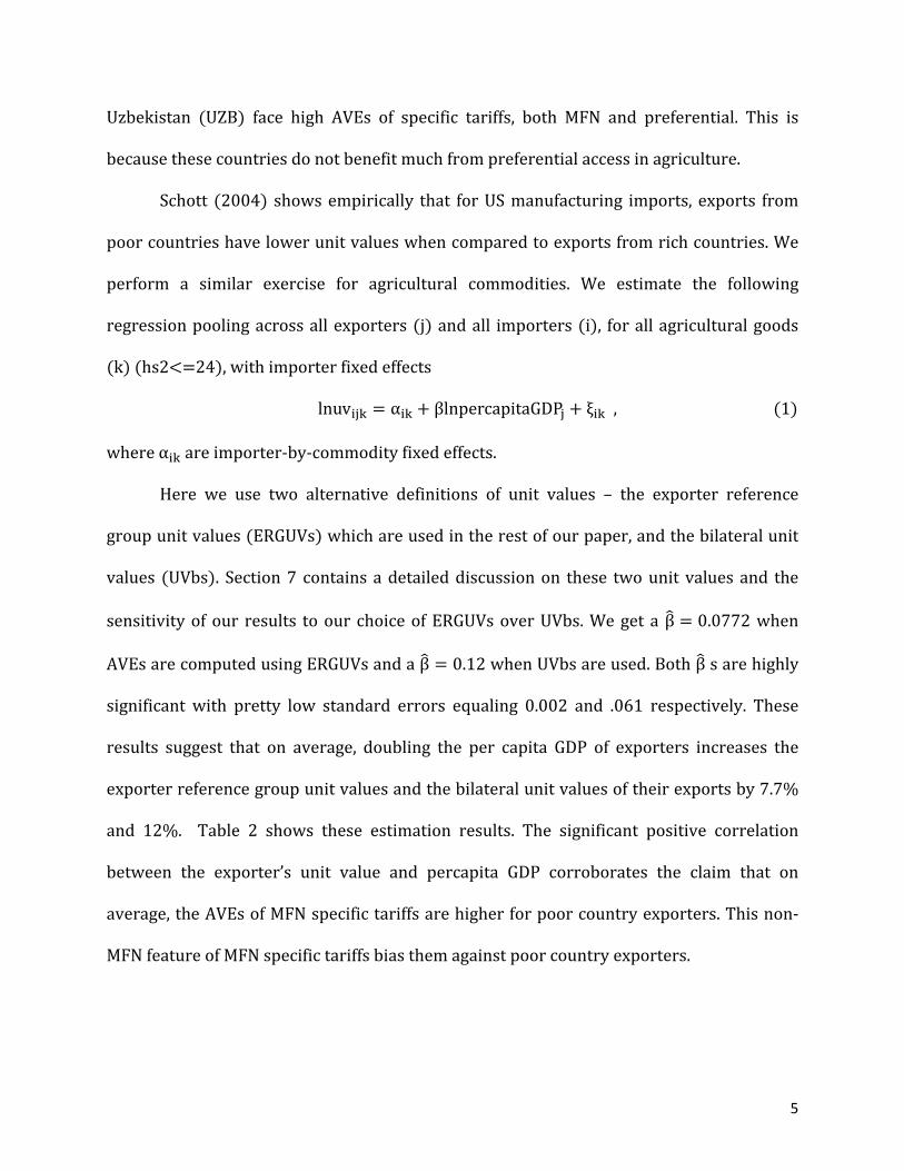
Uzbekistan (UZB) face high AVEs of specific tariffs, both MFN and preferential. This is because these countries do not benefit much from preferential access in agriculture. Schott (2004) shows empirically that for US manufacturing imports, exports from poor countries have lower unit values when compared to exports from rich countries. We perform a similar exercise for agricultural commodities. We estimate the following regression pooling across all exporters (j) and all importers (i), for all agricultural goods (k) (hs2<=24), with importer fixed effects lnuv = α + βlnpercapitaGDP + ξ , (1) where α are importer-by-commodity fixed effects. Here we use two alternative definitions of unit values – the exporter reference group unit values (ERGUVs) which are used in the rest of our paper, and the bilateral unit values (UVbs). Section 7 contains a detailed discussion on these two unit values and the sensitivity of our results to our choice of ERGUVs over UVbs. We get a β = 0.0772 when AVEs are computed using ERGUVs and a β = 0.12 when UVbs are used. Both β s are highly significant with pretty low standard errors equaling 0.002 and .061 respectively. These results suggest that on average, doubling the per capita GDP of exporters increases the exporter reference group unit values and the bilateral unit values of their exports by 7.7% and 12%. Table 2 shows these estimation results. The significant positive correlation between the exporter’s unit value and percapita GDP corroborates the claim that on average, the AVEs of MFN specific tariffs are higher for poor country exporters. This non-MFN feature of MFN specific tariffs bias them against poor country exporters.

6

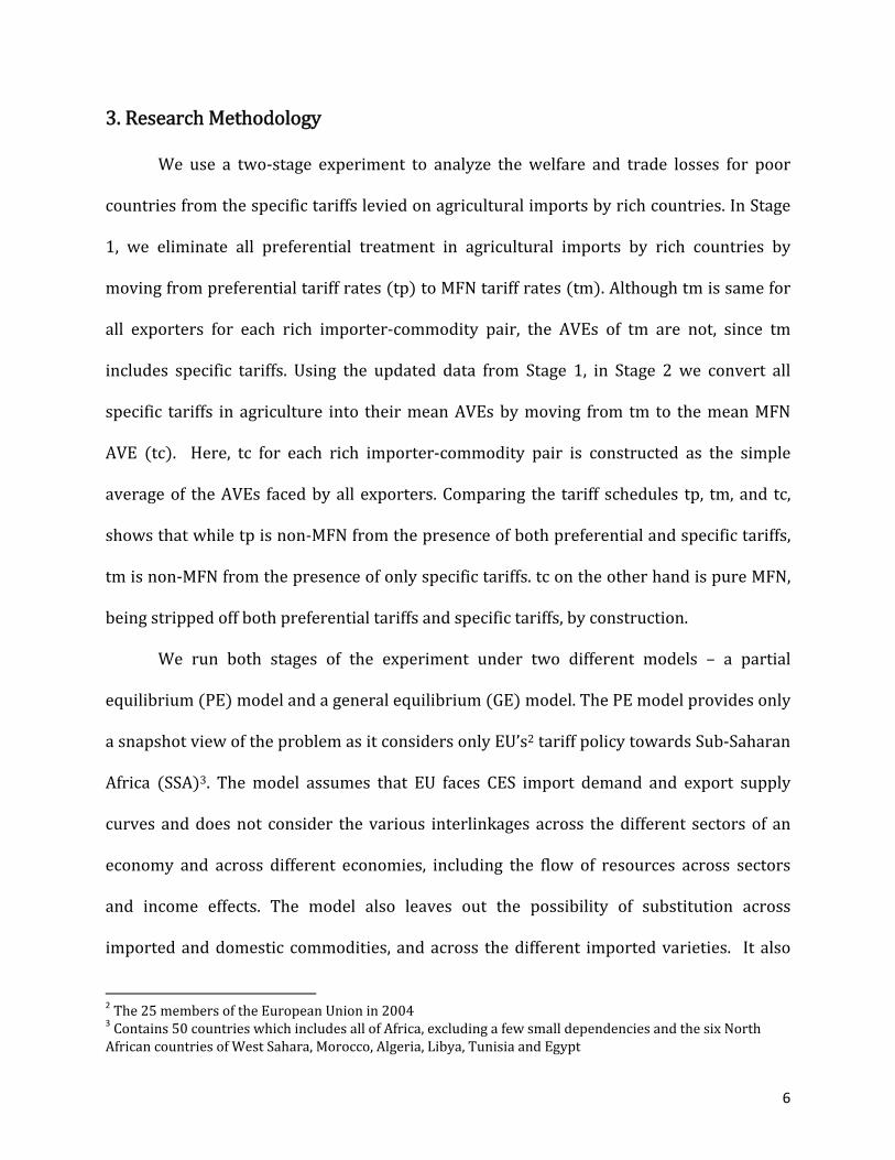
3. Research Methodology We use a two-stage experiment to analyze the welfare and trade losses for poor countries from the specific tariffs levied on agricultural imports by rich countries. In Stage 1, we eliminate all preferential treatment in agricultural imports by rich countries by moving from preferential tariff rates (tp) to MFN tariff rates (tm). Although tm is same for all exporters for each rich importer-commodity pair, the AVEs of tm are not, since tm includes specific tariffs. Using the updated data from Stage 1, in Stage 2 we convert all specific tariffs in agriculture into their mean AVEs by moving from tm to the mean MFN AVE (tc). Here, tc for each rich importer-commodity pair is constructed as the simple average of the AVEs faced by all exporters. Comparing the tariff schedules tp, tm, and tc, shows that while tp is non-MFN from the presence of both preferential and specific tariffs, tm is non-MFN from the presence of only specific tariffs. tc on the other hand is pure MFN, being stripped off both preferential tariffs and specific tariffs, by construction. We run both stages of the experiment under two different models – a partial equilibrium (PE) model and a general equilibrium (GE) model. The PE model provides only a snapshot view of the problem as it considers only EU’s2 tariff policy towards Sub-Saharan Africa (SSA)3. The model assumes that EU faces CES import demand and export supply curves and does not consider the various interlinkages across the different sectors of an economy and across different economies, including the flow of resources across sectors and income effects. The model also leaves out the possibility of substitution across imported and domestic commodities, and across the different imported varieties. It also 2 The 25 members of the European Union in 2004 3 Contains 50 countries which includes all of Africa, excluding a few small dependencies and the six North African countries of West Sahara, Morocco, Algeria, Libya, Tunisia and Egypt

7

leaves out interactions between the import tariffs and preexisting taxes on output, endowment, consumption and exports. The elements that the PE model leaves out are captured in the computable general equilibrium Global Trade Analysis Project (GTAP) model (Hertel, 1997), which analyzes simultaneously the trade policy of multiple importers and exporters. But these merits of the general equilibrium (GE) model come at a cost – the high level of region and commodity aggregation underlying the model covers up some effects which are otherwise transparent in an analysis done at the tariff line with individual countries. These effects include compositional effects, where the average tariff faced by an exporter is determined by the composition of its exports due to the multiple tariff lines existing within each aggregate commodity group. In this sense, the PE and GE models are complementary. We discuss the PE model in the following section and the GE model in Section 5. 4. PE Model In this model we compute the percentage of benefits enjoyed by SSA from EU preferential tariffs on agriculture that are taken away by EU specific tariffs on agriculture. We consider EU to be the only importing country, exporting to all other countries. In Stage 1, we eliminate preferential tariffs by EU on its agricultural imports from SSA by moving from tp to tm. The resulting welfare change in each region is given by differences in the DWLs corresponding to tp and tm. In Stage 2 we eliminate all specific tariffs on agricultural imports by EU by moving from tm to tc and the resulting welfare change in each region is given by differences in the DWLs between tc and tm. The importer’s and exporter’s DWLs from tariff rate t are computed as discussed below.

8

The model assumes that EU faces CES import demand and export supply curves. This import demand curves for EU imports are given by q = adjkp−σk (2) The export supply curves faced by EU are given by q = asjkpSk (3) Where, j is an exporter index, k is a good index, σk is the import demand elasticity of substitution between the various Armington import varieties of good k, and S is the price elasticity of supply of exports of good k from the rest of the world as faced by EU. a and a are shift parameters corresponding to the import demand and export supply curves respectively. From the Comtrade dataset, we obtain data on the bilateral c.i.f prices (p ) and import quantitities (q ) for the EU. All other prices and quantities are expressed in terms of these values and elasticities. The import tariff introduces a wedge between prices paid by domestic consumers and prices received by foreign suppliers as p = p 1 + t (4) The distribution of tariff incidence between EU and SSA is determined by the import demand and export supply elasticities σ and S . The values of a and a are computed from 2) and 3) respectively using the available data as a = q p (5) a = q p S (6) We obtain the welfare and trade changes corresponding to the exporter and importer from a tariff rate t, from the areas of the harberger’s triangle as shown in the Appendix. To obtain the welfare changes accruing to EU and SSA from Stages 1 and 2 of our

9

experiment, we compare the DWLs corresponding to the three tariff schedules tp, tm, and tc. For the PE model, we use hs6-commodity-level disaggregated EU bilateral import and tariff data sourced from the Comtrade and MAcMap-HS6v2.02 database respectively. Both data sets correspond to the year 2004. While the Comtrade dataset provides information on import values and quantities, the MAcMap-HS6 database provides information on the advalorem and specific components of MFN (tm) and preferential (tp) tariff rates, for a set of 163 importers, 208 exporters and 5113 hs6 commodities. The dataset also contains data on different unit values – bilateral, importer, exporter and exporter reference group (ERGUV). We construct the AVEs of specific tariffs by dividing specific tariffs by ERGUVs. We discuss the sensitivity of our results to the choice of unit values used in computing AVEs in Section 7. The mean advalorem tariff equivalent (tc) for each importer-commodity pair is constructed as the trade weighted average of all AVEs, averaged over all exporters. We obtain values for the hs6-commodity-specific import demand elasticity of substitution for EU from Broda and Weinstein (2006). Further, we assume that the commodity-specific price elasticity of export supply faced by EU are the same as those faced by the US, and obtain these elasticities from Broda, Limao and Weinstein (2008). Table 8 shows the welfare changes from Stages 1 and 2. In Stage 1, when EU removes all preferential tariffs on its agricultural imports from SSA, both EU and SSA face allocative efficiency (AE) losses. This is because the removal of preferences is equivalent to a move to higher MFN tariffs. These higher tariffs generate a TOT gain for EU and a corresponding TOT loss for SSA. The numerical values of these losses show that the TOT

10

effects pale in comparison to the AE effects suggesting that the supply curve faced by EU on agriculture exports from SSA is relatively flat. In other words, EU does not wield significant market power. In Stage 2 we eliminate specific tariffs on EU imports of agriculture from SSA. Our results indicate that SSA gains in terms of both AE and TOT since it now faces lower tariff rates. The EU on the other hand faces a loss in terms of both AE and TOT. This is because levying mean advalorem AVE tariffs on all exporters increases the average tariffs levied by the EU, since AVEs on SSA are much higher that than AVEs on other rich exporters. These rich exporters now also face higher tariffs, and higher AE and TOT loss. The combined results from Stages 1 and 2 suggest that 65% of the welfare gains and 56% of the trade gains enjoyed by SSA from preferential tariffs on its agricultural exports to EU are taken away by specific tariffs imposed by EU. These welfare and trade losses to SSA from EU specific tariffs are equivalent to 7.4% and 39% respectively, of SSA agriculture exports to the EU as seen in Table 3. This simple model provides only a snapshot view of the problem for reasons discussed in Section 3. The GTAP GE model discussed in the next section provides a more holistic view, but at the cost of higher aggregation. 5. GE Model 5.1 GTAP Model and Experiment The GTAP model is a comparative static, global computable general equilibrium model based on neoclassical theories. The model assumes perfect competition in all markets, constant returns to scale in all production and trade activities, and profit and utility maximizing behavior of firms and households respectively. The model includes:

11

demand for goods for final consumption, intermediate use and government consumption, demands for factor inputs, supplies of factor and goods, and the international trade of goods and services. Bilateral international trade flows are handled using the Armington assumption in which products are exogenously differentiated by origin (Armington, 1969). In the standard closure, global investment adjusts to global savings so that the national balances of payments are endogenous. The model is solved using the GEMPACK software (Harrison and Pearson, 1996). Full documentation of the GTAP model and database can be found in Hertel (1997) and also in Narayanan and Walmsley (2008). The GTAP model is complemented by the GTAP version 7 database which contains the same data as in our PE model, but aggregated to 113 regions and 57 commodities. In addition to trade and tariff data, the GTAP database also contains data on domestic taxes, production, Armington substitution elasticities, and substitution elasticities between domestic goods and imports. For ease of application, we further aggregate the GTAP database into our user level of aggregation (shown in Table 5) of 11 commodities – 9 agricultural commodities (cereal, vegetable, cattle, animal products, dairy, vegetable oil, tobacco and beverages, sugar, other agriculture), manufacturing and service, and 7 regions – USA, EU (the 25 EU members in 2004), JPNSEA (Japan, Hong Kong, Malaysia, Singapore, Taiwan, Korea), XOD (other developed countries), India, China, SSA (Sub-Saharan Africa), XLC (other low income countries) and XDC (other developing countries). Regarding tariffs, the GTAP database contains data only on preferential applied tariff rates (tp) obtained from MAcMap, aggregated to the GTAP level. But we also require data on MFN applied tariff rates (tm) for our analysis. We obtain this from MAcMap at the hs6 level of commodity aggregation and aggregate it to our user level of aggregation using trade weighted means.

12

The mean advalorem tariff rates (tc) are obtained at the hs6 level of commodity aggregation and aggregated to our user level of aggregation using trade weighted means. A closure in a general equilibrium model specifies the variables in the model as either exogenous or endogenous. In our model, we modify the standard GTAP GE closure to account for the possibility of unemployment of unskilled labor in poor regions (CHN+IND+SSA+XLC+XDC). We make this alteration to reflect more accurately the labor markets in these poor regions which are typically characterized by an excess supply of unskilled labor. Since this excess labor can be drawn on by industries in the event of increased production, an assumption of full employment is inappropriate for these countries. We achieve this modification by fixing the real wage rate of unskilled labor and endogenizing the supply of labor in these poor regions of the world. This allows us to take into account the effect of unemployment within poor regions following a tariff change. In this context, there is also a section of the literature on CGE modeling which debates on the pros and cons of running a liberalization scenario while holding fixed the ratio of trade balance to regional income through endogenizing the ratio of saving to regional income (McDonald and Walmsely, 2003). The idea behind this debate is that since an endogenous trade balance (like in the standard closure) generates current account changes following tariff changes, tariff change scenarios are accompanied by compensating capital inflows/outflows which over/under estimate the gains from tariff changes (McDonald and Van Tongeren). So some modelers prefer to fix the ratio of trade balance to income to avoid these over/under estimations. But in our model we work with the standard endogenous trade balance assumption.

13

5.2 Results: Welfare Changes The GTAP model uses the Equivalent Variation (EV) as the money metric measure of welfare changes. Following Huff and Hertel (2000) and Hertel et al (2006),

EV(s) = (Ψ )

⎩⎪⎪⎪⎪⎪⎪⎪⎪⎪⎪⎪⎨⎪⎪⎪⎪⎪⎪⎪⎪⎪⎪⎪⎧ tM PCIF dQMSRN + tX PFOB dQXSRN

+ t PO dQON + t CD PPCD dQPCDN

+ t CM PPCM dQPCMN + tGCD PGCD dQGCDN

+ tGCM PGCM dQGCMN + tE PE dQERN

+ tIM PIM dQIMRN + tID PID dQIDRN

+ QMS dPFOBRN − QMS dPCIFRNTOT EffectVOA dQOM + (NETINV PCGDS − SAVE PSAVE )

EE Effect I − S Effect ⎭⎪⎪⎪⎪⎪⎪⎪⎪⎪⎪⎪⎬⎪⎪⎪⎪⎪⎪⎪⎪⎪⎪⎪⎫

(7) where, s indexes regions and Ψ is a scaling factor specific to region s which is initially normalized to one, but changes as a function of the marginal cost of utility in the presence of non-homothetic preferences (McDougall, 2002). Changes in initial capital stock, population and technology are assumed to be zero. Equation 7 shows that the regional welfare changes can be decomposed into the Allocative Efficiency Effect (AE), the TOT Effect (TOT), the Endowment Effect (EE) and the Investment-Savings (IS) Effect. The AE effect on regional EV is attributed to interactions between taxes (both pre-existing and

AE Effect

14

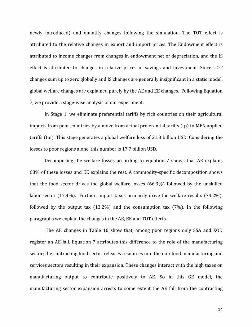
newly introduced) and quantity changes following the simulation. The TOT effect is attributed to the relative changes in export and import prices. The Endowment effect is attributed to income changes from changes in endowment net of depreciation, and the IS effect is attributed to changes in relative prices of savings and investment. Since TOT changes sum up to zero globally and IS changes are generally insignificant in a static model, global welfare changes are explained purely by the AE and EE changes. Following Equation 7, we provide a stage-wise analysis of our experiment. In Stage 1, we eliminate preferential tariffs by rich countries on their agricultural imports from poor countries by a move from actual preferential tariffs (tp) to MFN applied tariffs (tm). This stage generates a global welfare loss of 21.3 billion USD. Considering the losses to poor regions alone, this number is 17.7 billion USD. Decomposing the welfare losses according to equation 7 shows that AE explains 68% of these losses and EE explains the rest. A commodity-specific decomposition shows that the food sector drives the global welfare losses (66.3%) followed by the unskilled labor sector (17.4%). Further, import taxes primarily drive the welfare results (74.2%), followed by the output tax (13.2%) and the consumption tax (7%). In the following paragraphs we explain the changes in the AE, EE and TOT effects. The AE changes in Table 10 show that, among poor regions only SSA and XOD register an AE fall. Equation 7 attributes this difference to the role of the manufacturing sector; the contracting food sector releases resources into the non-food manufacturing and services sectors resulting in their expansion. These changes interact with the high taxes on manufacturing output to contribute positively to AE. So in this GE model, the manufacturing sector expansion arrests to some extent the AE fall from the contracting

15

food sector. The AE losses in poor regions are driven primarily by the falling exports of food interacting with the lack of export subsidies on food in these regions, and the contraction of the domestic food sector. Although resources released from the food sector get absorbed in the non-food sectors, output of the non-food sectors is not allowed to increase by the PE closure. This is possible through a reduction in the productivity of all resources employed in the non-food sector. In rich regions, AE losses are attributed to the high subsidies on food exports interacting with the slight increase in food exports. The EE effects in Table 10 show that poor regions face welfare losses in Stage 1 from the falling employment of unskilled labor. On the other hand, there is no change in endowment income in rich regions since the aggregate output of all endowments, including unskilled labor, are held fixed in these regions. In poor regions, the removal of preferential tariffs generates a drop in the employment of unskilled labor. This is because for these net exporters of food, removal of preferential tariffs lowers their food exports, contracting their domestic food sector. The contracting food sector releases unskilled labor, some of which gets absorbed in manufacturing and services. Table 10 shows that the drop in employment of unskilled labor in poor regions contributes 6.8 billion USD to the EV loss in these regions. The food sector contraction when multiplied by the initial income from unskilled labor generates an income loss from the falling employment of unskilled labor. Tracing this income fall to the sectors of economy shows that most of this income fall is from the unskilled labor displaced from the contracting food sector. The TOT effect contributes negatively to the welfare of poor regions since every poor region witnesses a fall in export prices and a rise in import prices as seen in Table 13. The situation is reversed in rich regions excepting in JPNSEA and US where import prices

16

rise, but relatively less than export prices. The export price changes are driven primarily by the manufacturing sector which explains 64% of the changes. The food and services sector account for 17.8% and 18% respectively. The manufacturing sector contributes even more to import price changes, explaining 70.2% of the changes, with the food sector accounting for 31.4%. In Stage 2 we eliminate all specific tariffs by rich countries on their agricultural imports by a move from MFN applied tariffs (tm) to mean AVE tariffs (tc). This stage generates a global welfare loss of 4.47 billion USD. Considering the losses accruing to poor regions alone, this number is 14.18 billion USD. AE rises in all poor regions, excepting in China where it falls slightly. This fall in AE is on account of the contracting manufacturing sector. The contracting manufacturing sector creates a fall in demand for resources used in manufacturing which interacts with the high taxes on these resources and the high tax on manufacturing output to contribute negatively to the AE. Like in Stage 1, import taxes drive the AE changes in poor regions. As discussed earlier, the positive endowment effect arises from the unemployed unskilled labor getting drawn into the expanding agricultural sector in poor regions. The cumulative results from Stages 1 and 2 of the GE model show that 80% of the welfare benefits enjoyed by poor countries from the preferences granted on their agriculture exports to rich countries, are taken away by the specific tariffs levied by rich countries (Table 12). The lack of data makes it impossible to differentiate between preferential tariffs resulting from unilateral and bilateral trade agreements. But following our experiment methodology, it is safe to say that our experiment results will be stronger if considering unilateral tariffs alone. This is because in Stage 1, we remove all preferential

17

tariffs on rich country imports of agricultural commodities from poor countries. But in a bilateral trade agreement, there are also preferential tariffs on poor country imports of rich country exports which are we keep unchanged in our experiment. So our Stage 1 results are higher, in a bilateral agreement where the preference flowing from poor to rich countries are not simultaneously removed. But in a unilateral trade agreement, there are no preferences flowing from poor to rich countries. So considering the removal of only unilateral preferences would generate lower Stage 1 results. Since the Stage 2 results are the same in both cases, the percentage of benefits lost by poor countries (column 3 of Table 12) would be higher if we consider only unilateral preferences. 5.3 Results: Trade Balance Changes Our results show that specific tariffs wash away 73% of the market access poor countries gain in agriculture from preferential tariffs. The change in trade balance (in million USD) corresponding to region s from trade in food is given by the difference between the change in the value of the regional merchandise exports and imports, weighted by the value of these exports and imports. The results from our experiment (Figure 6) show that in the trade of agriculture, Stage 1 generates a trade balance loss for poor countries who are net agriculture exporters, and a trade balance gain for rich countries who are net agricultural importers. The situation is reversed in Stage 2. DTBAL , = VXW , ∗ vxwfob , − VIW , ∗ viwcif , (8)

18

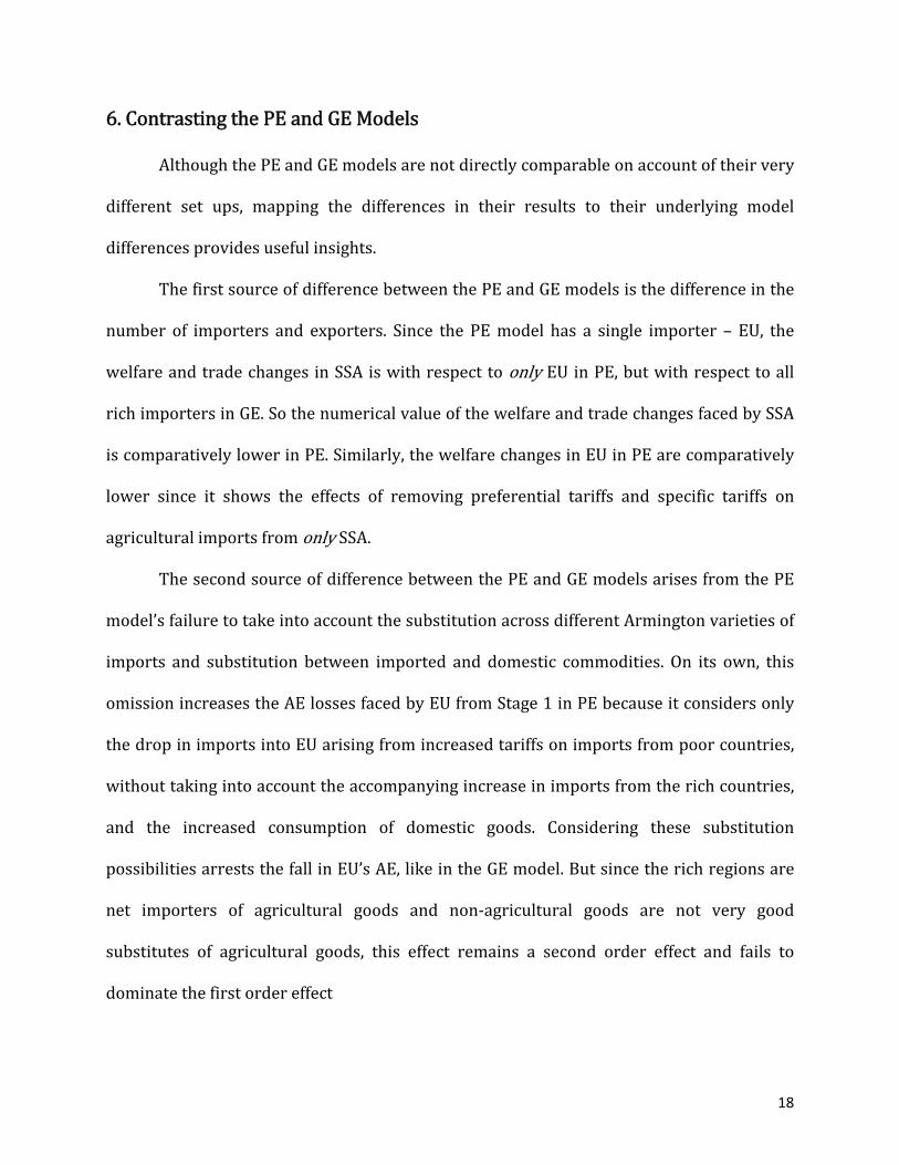
6. Contrasting the PE and GE Models Although the PE and GE models are not directly comparable on account of their very different set ups, mapping the differences in their results to their underlying model differences provides useful insights. The first source of difference between the PE and GE models is the difference in the number of importers and exporters. Since the PE model has a single importer – EU, the welfare and trade changes in SSA is with respect to only EU in PE, but with respect to all rich importers in GE. So the numerical value of the welfare and trade changes faced by SSA is comparatively lower in PE. Similarly, the welfare changes in EU in PE are comparatively lower since it shows the effects of removing preferential tariffs and specific tariffs on agricultural imports from only SSA. The second source of difference between the PE and GE models arises from the PE model’s failure to take into account the substitution across different Armington varieties of imports and substitution between imported and domestic commodities. On its own, this omission increases the AE losses faced by EU from Stage 1 in PE because it considers only the drop in imports into EU arising from increased tariffs on imports from poor countries, without taking into account the accompanying increase in imports from the rich countries, and the increased consumption of domestic goods. Considering these substitution possibilities arrests the fall in EU’s AE, like in the GE model. But since the rich regions are net importers of agricultural goods and non-agricultural goods are not very good substitutes of agricultural goods, this effect remains a second order effect and fails to dominate the first order effect

19

The third source of difference between the PE and GE models arises from the PE model’s failure to take into account the input markets and the interaction of import tariffs with other preexisting taxes like export subsidies, output taxes, consumption taxes and input taxes. The role of these interactions in determining the welfare losses in the GE model is shown by all the terms following the first term in Equation 7. 7. Sensitivity of Results Our experiment results are sensitive to our choice of unit values used in computing the AVEs of specific tariffs. This is because the greater the dispersion in the within-commodity cross-exporter unit values, the greater will be the distortionary effects of specific tariffs, particularly the bias against poor countries in the form of higher AVEs. We use the exporter’s reference group unit values (ERGUVs) to compute AVEs. Since the ERGUVs are computed as the median unit value of worldwide exports from an exporter’s reference group (Bouet et al, 2001), they have a lower dispersion than the bilateral unit values (UVbs), as seen from Figure 5. This suggests that using UVbs instead of ERGUVs would generate higher specific tariffs-induced welfare and trade surplus losses for poor regions. In other words, the losses from specific tariffs obtained from the PE and GE models are the lower bounds of a possible range of losses from using different unit values. This makes our result stronger. The sensitivity of our results from the PE and GE models is also checked with respect to the value of two crucial parameters – the elasticity of substitution between imported Armington varieties (ESUBM) in agriculture, and the elasticity of substitution between domestic and composite imported varieties (ESUBD) in agriculture. But since in

20

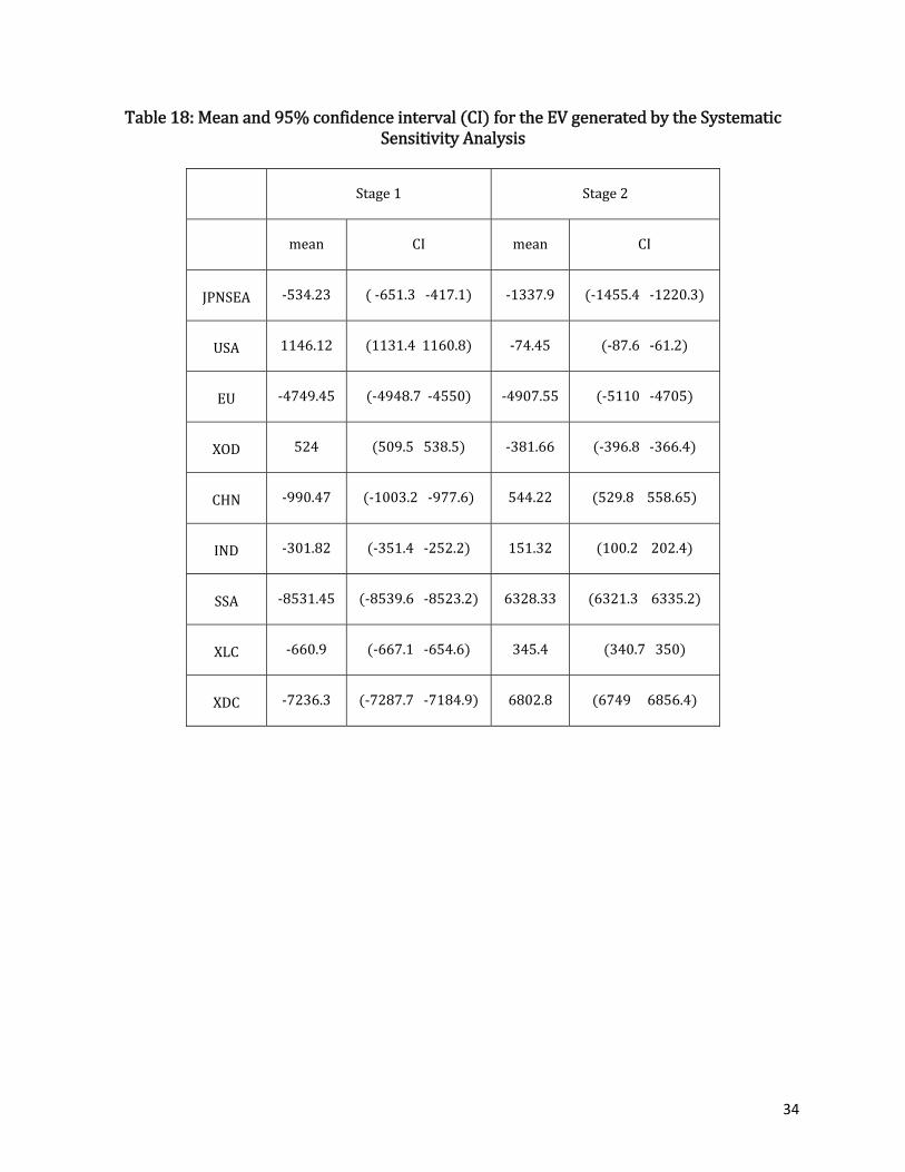
the GTAP model ESUBM is derived as twice the value of ESUBD, a x% change in ESUBD is equivalent to a x% change in ESUBM. Table 18 shows the confidence intervals within which the EV changes vary when the values of ESUBD (and therefore ESUBM) for all traded commodities are varied independently by 50% in either direction from their base values. Table 17 shows the limits within which the ESUBD and ESUBM values are varied. The sensitivity analysis results suggest that for the GE model, the variation in EV resulting from varying the elasticity parameters are not high enough to change the results of our experiment qualitatively. This is true for both stages of the experiment, indicating that our results are robust to the choice of elasticity parameters. 8. Conclusions Our paper contributes to the literature on the distortions associated with specific tariffs. This is the first attempt at quantifying the costs of these distortions borne by poor countries. Specific tariffs discriminate against exports from poor countries through two channels. First, poor countries export lower priced goods which translate into higher advalorem equivalents (AVEs) for the same specific tariff. Second, specific tariffs are concentrated in agricultural goods, the bulk of which are supplied by poor countries. So, the MFN specific tariffs levied by rich WTO member countries essentially translate into higher tariff barriers for the exporters of low price goods, suggesting that the preferential tariff benefits enjoyed by poor countries might be offset by the specific tariff losses. We investigate this issue using both a partial equilibrium (PE) model and a computable general equilibrium (GE) GTAP model. The PE model provides a snapshot view of the problem by ignoring the cross-sector and cross-economy linkages, the input markets, the services

21

sectors and the interaction between taxes. These linkages are addressed in the GE model, providing a more holistic view of the problem. But the merits of the GE model come at a cost – the high level of commodity and region aggregation underlying the GE model covers up effects which are otherwise transparent in an analysis performed at the tariff line level for each individual country. The results of my analysis suggest that the WTO should intensify efforts to eliminate specific tariffs in agriculture. This is because the distortions from specific tariffs on rich country agricultural imports wash away 80% of the welfare and 73% of the market access benefits poor countries enjoy from preferential tariffs. 9. References Alchian, A., Allen, William R. University Economics. Belmont, CA: Wadsworth Publishing Company, 1964 Armington, P.S., 1969. “A theory of demand for products distinguished by place of production”, IMF Staff Papers 16 (2), 179–201. Badri Narayanan G., Terrie L. Walmsley, (Editors), “Global Trade, Assistance, and Production: The GTAP 7 Data Base”, Center for Global Trade Analysis, Purdue University, 2008 Boorstein R., Feenstra R. “Quality upgrading and its welfare costs in US steel imports 1969-74”, NBER working paper no. W2452 Bouet, A et al “A Consistent, Advalorem Equivalent measure of Applied Protection across the world: The MAcMap-HS6 database”, CEPII, working Paper no. 2004-22(2004) Boumellassa H., Laborde, D., Mitaritonna, C. “A consistent picture of the protection across the world in 2004: MAcMapHS6 version 2”, IFPRI Discussion paper. 2009 Broda, C., Weinstein, D.E. “Globalization and the Gains from Variety”, QJE, 121(2) 2006 Broda, C., Limao, N., Weinstein, D.E. “Optimal Tariffs and Market Power: The Evidence”, AER 98(5) 2008 Bureau, J. & Salvatici, L. “Agricultural Trade Restrictiveness in the EU and US”, IIIS Discussion Paper No. 59, Jan 2005

22

Gibson et al “Profiles of Tariffs in Global Agricultural markets “USDA, Agricultural Economic Report 796 (2001) Harrison, J.W., Pearson, K.R. “Computing Solutions for large General Equilibrium Models using GEMPACK”, Computational Economics, 1996 Hertel, T.W., Hummels, D., Ivanic, M., Keeney, R. “How Confident can we be of CGE-based assessments of Free Trade Analysis?”, Economic Modeling 24(2007) Hertel, T.W. “Global Trade Analysis: Modeling and Applications”, Cambridge University Press, 1997 Huff, K., Hertel, T., 1996., “Decomposing Welfare Changes in GTAP,” GTAP Technical Paper No. 5, Center for Global Trade Analysis, Purdue University, West Lafayette, IN. (revised 2001). Horridge, J.M. and Laborde, D., “TASTE: a program to adapt detailed trade and tariff data to GTAP-related purposes”, GTAP Technical Paper, Centre for Global Trade Analysis, Purdue University, 2008 Laborde, D., ‘Mesures et détermination endogène des droits de douane’ Ph.D. thesis, Université de Pau et des Pays de l'Adou,. 2008 McDonald, S., Van Tongeren, F., “Alternative Closures in GTAP” GTAP Short Course Lecture McDonald, S., Walmsely, T. "Bilateral Free Trade Agreements and Customs Unions: The Impact of the EU Republic of South Africa Free Trade Agreement on Botswana", GTAP Working Paper no. 29, Center for Global Trade Analysis (2003) McDougall, R.A., 2002., “A New Regional Household Demand System for GTAP”, GTAP Technical Paper, vol. 20. Global Trade Analysis Project, Purdue University Narayanan, B., Walmsely, T., “GTAP 7 Base Data Documentation”, Center for Global Trade Analysis, 2008 Schott, P. “Across-Product versus Within-Product Specialization in International Trade”, QJE, 119(2), 2004 Von Kirchbach, F., Mondher, M. “Market Access Barriers: A Growing Issue for Developing Country Exporters”, International Trade Forum, Issue 2/2003 (2003)

23

10. Figures and Tables Figure 1: Distribution of the AVEs of specific tariffs across hs2 commodity categories, for all importers

hs2=6 live trees and plants hs2 =24 tobacco Figure 2: Distribution of MFN Specific tariff rates in Agriculture across Importers

Note: (ISL, 19%) says that 19% of the global specific tariff rates (in USD per ton) in agriculture is levied by Iceland on its imports VUT: Vanatau BRN: Brunei MYS: Malaysia UKR: Ukraine BMU: Bermuda CHE: Switzerland NOR: Norway JPN: Japan

24

Figure 3: Preferential Specific tariffs vs MFN Specific tariffs in Agriculture by Importers

Figure 4: AVE of MFN Specific Tariffs vs AVE of Preferential Specific Tariffs in Agriculture by Exporter

KEN: Kenya KGZ: Kazakhstan UZB: Uzbekistan VNM: Vietnam PNG: Papua New Guinea MNG: Mongolia

25

Figure 5: Plot comparing the dispersion of ERGUVs and UVbs for each agricultural hs6 tariff line

Figure 6: Trade Surplus changes (in USD million) in agriculture in GE

Table 1: Distribution of bilateral tariff lines with positive specific tariffs, across agricultural and non-agricultural commodities bilateral tariff lines(1) bilateral tariff lines with positive specific tariffs (2) (1) as a % of (2)agricultural commodities 4,112,329 455,888 11%non-agricultural commodities 48,853,870 825,358 1.6%Total 52,966,199 1,281,246 2.4%

-40000

-30000

-20000

-10000

0

10000

20000

30000

JPN

SEA

USA EU

XOD

CHN

IND

SSA

XLC

XDC

Stage 1

Stage 2

26

Table 2: Results from the fixed effects regression of ln(ERGUV) and ln(UVb) separately, on ln(percapita GDP), pooling across all importers and exporters with importer fixed effects, for all agricultural commodities statistic dependent variable =ln(AVE_ERGUV) dependent variable = ln(AVE_UVb) no. of observations 229640 229640 𝛽 0.0772 0.12 standard errors, pvalue 0.002, 0.00 0.061, 0.00 Table 3: Agriculture imports (in USD billion) from SSA and the specific tariffs on these imports importer imports MFN specific tariffs(%) preferential specific tariffs (%)EU 9.67 31.3 23.8USA 1.2 14.7 12.2Japan .79 28.2 27.7World 18.6 10 6.2 Table 4: Tariff rates (in %) in the PE Model tp tm tc

Importer EU 15 25.8 23.9

Exporters SSA 23.8 31.3 27.7

Non-SSA 19.5 25 23.4

27

Table 5: Model Resources, Sectors and Regions Resources Sectors Regions Land Skilled Labor Unskilled Labor Capital cerealvegetablecattle animal products vegetable oils dairy sugar tobacco&beverages other agri manufacturingservices

JPNSEA USA EU XOD CHN IND SSA XLC XDC

rich countries

Table 6: The importer’s and exporter’s welfare and trade surplus losses in the PE model DWL faced by EU from all commodities and all exporters DWLEU(t) =

a p 1σ − 1 + 1 + t S S − σσ − 1 1 + t S ( )S Allocative Efficiency Loss − a p 1 + t S S 1 − 1 + t S TOT LossDWL faced by exporter j from all commodities DWL (t) =

a p S(S + 1) 1 + t (S )S + 1(S + 1) − 1 + t S SAllocative Efficiency Loss + a p 1 + t S S 1 − 1 + t S TOT LossImport value losses faced by EU from all commodities and all exporters ΔXEU(t) =

a p 1 + t SS − 1𝒌 Export value losses faced by exporter j from all commodities ΔX (t) =

a p 1 + t SS − 1

poor countries

agriculture

28

Table 7: DWLs corresponding to some special scenarios, based on the formulae in Table 6 Scenario Result

When t = 0, for all j, k TOT loss and allocative efficiency loss for the EU is 0 TOT loss and allocative efficiency loss for each exporter is 0 DWL for both importer and exporters is 0 Although DWL = 0, welfare is not optimum for the EU since DWL can be positive from positive TOT gains Export value losses for each exporter is 0

When S = ∞ for all k, indicating a flat export supply curve faced by the EU, The TOT gains for the EU and TOT losses for each exporter is 0 When σ = ∞, for all k, indicating a flat import demand curve faced by the EU Allocative Efficiency loss for EU is 0 Table 8: The decomposition of the DWL changes (in USD million) accruing to EU and SSA under the PE model AE change TOT change DWL change

Stage 1 Stage 2 Stage 1 Stage 2 Stage 1 Stage 2 EU -2850 569.90 140 -83 -2710 486 SSA -992 509 -140 189 -1132 698

29

Table 9: Export value losses (in USD million) in agriculture in EU and SSA in PE trade surplus losses

Stage 1 Stage 2EU 6802 -3067SSA -6802 2336 Table 10: AE changes in GE (in USD million)

Region AE EE TOT Stage 1 Stage 2 Stage 1 Stage 2 Stage 1 Stage 2 JPNSEA -1820.5 -838.23 0 0 1302.03 -510.91

USA -70.3 -109.6 0 0 1213.2 -212.84 EU -7950.2 -250.8 0 0 3200.44 -5032.38

XOD -160.36 -655.1 0 0 677.87 -273.34 CHN 278.76 -245.6 -406.43 269.43 -865.54 523.28 IND 97.5 83.78 -126.67 64.69 -266.33 167.23 SSA -3775.56 2407.76 -3004.65 2766.1 -1745.20 1003.57 XLC 14.32 152.6 -160.2 67.62633 -512.32 132.2 XDC -1103 376.45 -3117.4 2987.74 -3004.12 4203.23 Total -14489.52 921.45 -6815.35 6155.15 0.03 -0.04

30

Table 11: Total EV changes (in USD million) in GE Stage 1 Stage 2JPNSEA -534.44 -1338.85

USA 1146.34 -73.85EU -4750 -4906.55

XOD 523.84 -381.574CHN -989.87 544.75IND -302.72 152.718SSA -8532.66 6328.43XLC -661.45 345.604XDC -7236.9 6803.00Total -21337.86 4473.67 Table 12: EV changes (in USD billion) accruing to poor regions in GE

EV loss from Stage 1 EV gain from Stage 2 EV gain from Stage 2 as a % of EV loss from Stage 1 17.72 14.18 80

31

Table 13: Export and import price changes (in %) for agriculture in GE

Table 14: Output changes (in %) in agriculture in GE, Stage 1 Stage 2JPNSEA 1.72 0.12

USA 0.88 -0.07EU 2.05 -3.77XOD 2.83 -1.32CHN -1.25 0.90IND -0.46 0.33SSA -6.51 4.76XLC -2.76 2.00XDC -1.71 3.08Total -5.14 6.03

export price change import price changeStage 1 Stage 2 Stage 1 Stage 2JPNSEA 0.0065 -0.0004 0.0002 0.0071

USA 0.01447 -0.02148 0.00371 0.00041EU 0.0195 -0.00016 -0.00809 -0.00201

XOD 0.04364 -0.04461 -0.00525 0.00844CHN -0.01345 0.00348 0.00246 -0.00161IND -0.07084 0.00863 0.01447 -0.00528SSA -0.03789 0.01083 0.02531 -0.00737XLC -0.13419 0.05325 0.02236 -0.00558XDC -0.05912 0.0251 0.01147 -0.0011Total -0.23031 0.02768 0.06621 -0.00404

32

Table 15: Output changes (in %) in manufacturing and services in GE Stage 1 Stage 2manufacturing services manufacturing services JPNSEA -.33 -0.017 -0.31 0.002 USA -0.12 0.004 -0.29 0.008 EU -0.381 -0.032 0.691 0.064 XOD -0.655 -0.008 0.278 0.017 CHN 0.348 0.038 -0.251 -0.038 IND 0.799 0.128 -0.487 -0.084 SSA 1.219 -0.312 -0.980 0.241 XLC 2.129 0.051 -1.481 -0.063 XDC 0.817 -0.026 -0.938 0.021 Total 3.827 -0.175 -3.228 0.167 Table 16: Change (in %) in the employment of unskilled labor in GE Stage 1 Stage 2

JPNSEA 0 0USA 0 0EU 0 0XOD 0 0CHN -0.045 0.012IND -0.014 0.012SSA -1.76 1.66XLC -0.212 0.08XDC -0.38 0.44Total -2.41 2.20

33

Table 17: The limits within which the ESUBD values are varied for all traded commodity simultaneously traded commodities variation in ESUBDcereal 1.58 to 4.74vegetable 0.92 to 2.77cattle 1 to 3animal product 1.53 to 4.6vegetable oil 1.65 to 4.95dairy 1.8 to 5.4sugar 1.35 to 4.05tobacco & beverages 0.57 to 1.72other agri 1.14 to 3.42manufacturing 1.78 to 5.35services 0.95 to 2.85

34

Table 18: Mean and 95% confidence interval (CI) for the EV generated by the Systematic Sensitivity Analysis Stage 1 Stage 2

mean CI mean CI JPNSEA -534.23 ( -651.3 -417.1) -1337.9 (-1455.4 -1220.3)

USA 1146.12 (1131.4 1160.8) -74.45 (-87.6 -61.2) EU -4749.45 (-4948.7 -4550) -4907.55 (-5110 -4705)

XOD 524 (509.5 538.5) -381.66 (-396.8 -366.4) CHN -990.47 (-1003.2 -977.6) 544.22 (529.8 558.65) IND -301.82 (-351.4 -252.2) 151.32 (100.2 202.4) SSA -8531.45 (-8539.6 -8523.2) 6328.33 (6321.3 6335.2) XLC -660.9 (-667.1 -654.6) 345.4 (340.7 350) XDC -7236.3 (-7287.7 -7184.9) 6802.8 (6749 6856.4)

35

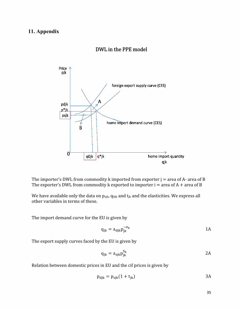
11. Appendix

DWL in the PPE model

The importer’s DWL from commodity k imported from exporter j = area of A- area of B The exporter’s DWL from commodity k exported to importer i = area of A + area of B We have available only the data on psjk, q0jk and tjk and the elasticities. We express all other variables in terms of these. The import demand curve for the EU is given by q = a p 1A The export supply curves faced by the EU is given by q = a pS 2A Relation between domestic prices in EU and the cif prices is given by p = p (1 + t ) 3A

36

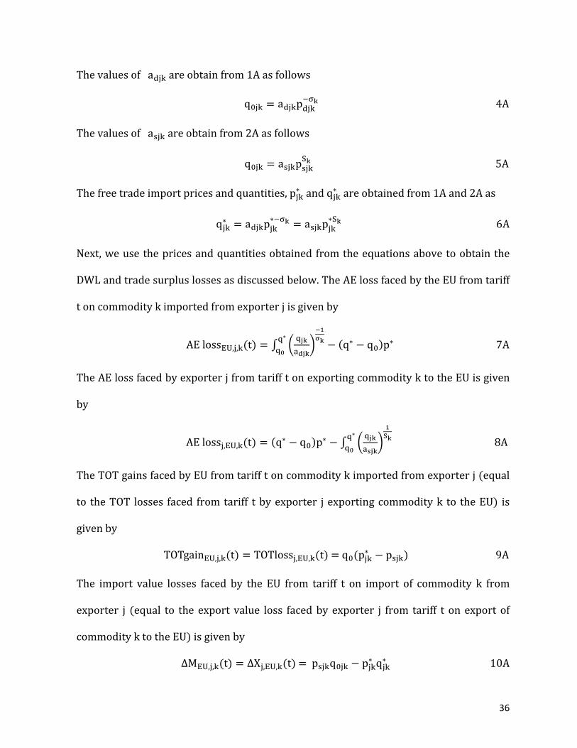
The values of a are obtain from 1A as follows q = a p 4A The values of a are obtain from 2A as follows q = a pS 5A The free trade import prices and quantities, p∗ and q∗ are obtained from 1A and 2A as q∗ = a p∗ = a p∗S 6A Next, we use the prices and quantities obtained from the equations above to obtain the DWL and trade surplus losses as discussed below. The AE loss faced by the EU from tariff t on commodity k imported from exporter j is given by AE lossEU, , (t) = ∫ ∗ − (q∗ − q )p∗ 7A The AE loss faced by exporter j from tariff t on exporting commodity k to the EU is given by AE loss ,EU, (t) = (q∗ − q )p∗ − ∫ S∗ 8A The TOT gains faced by EU from tariff t on commodity k imported from exporter j (equal to the TOT losses faced from tariff t by exporter j exporting commodity k to the EU) is given by TOTgainEU, , (t) = TOTloss ,EU, (t) = q (p∗ − p ) 9A The import value losses faced by the EU from tariff t on import of commodity k from exporter j (equal to the export value loss faced by exporter j from tariff t on export of commodity k to the EU) is given by ΔMEU, , (t) = ΔX ,EU, (t) = p q − p∗ q∗ 10A