the discontinuous enrichment method for a …ikalash/kalash_dissertation_june2011.pdf ·...
TRANSCRIPT

THE DISCONTINUOUS ENRICHMENT METHOD FOR
MULTI-SCALE TRANSPORT PROBLEMS
A DISSERTATION
SUBMITTED TO THE INSTITUTE FOR COMPUTATIONAL
AND MATHEMATICAL ENGINEERING
AND THE COMMITTEE ON GRADUATE STUDIES
OF STANFORD UNIVERSITY
IN PARTIAL FULFILLMENT OF THE REQUIREMENTS
FOR THE DEGREE OF
DOCTOR OF PHILOSOPHY
Irina Kalashnikova
June 2011

c© Copyright by Irina Kalashnikova 2011
All Rights Reserved
ii

Irina Kalashnikova
I certify that I have read this dissertation and that, in my opinion, it
is fully adequate in scope and quality as a dissertation for the degree
of Doctor of Philosophy.
(Charbel Farhat) Principal Adviser
I certify that I have read this dissertation and that, in my opinion, it
is fully adequate in scope and quality as a dissertation for the degree
of Doctor of Philosophy.
(Matthew F. Barone)
I certify that I have read this dissertation and that, in my opinion, it
is fully adequate in scope and quality as a dissertation for the degree
of Doctor of Philosophy.
(George C. Papanicolaou)
Approved for the University Committee on Graduate Studies.
iii

Abstract
A discontinuous enrichment method (DEM) for the efficient finite element solution
of advection-dominated transport problems in fluid mechanics whose solutions are
known to possess multi-scale features is developed. Attention is focused specifically on
the two-dimensional (2D) advection-diffusion equation −κ∆c(x)+a(x)·∇c(x) = f(x),
the usual scalar model for the Navier-Stokes equations. Following the basic DEM
methodology [1], the usual Galerkin polynomial approximation is locally enriched by
the free-space solutions to the governing homogeneous partial differential equation
(PDE). For the constant-coefficient advection-diffusion equation, several families of
free-space solutions are derived. These include a family of exponential functions that
exhibit a steep gradient in some flow direction, and a family of discontinuous poly-
nomials. A parametrization of the former class of functions with respect to an angle
parameter θi is developed, so as to enable the systematic design and implementation
of DEM elements of arbitrary orders. It is shown that the original constant-coefficient
methodology has a natural extension to variable-coefficient advection-diffusion prob-
lems. For variable-coefficient transport problems, the approximation properties of
DEM can be improved by augmenting locally the enrichment space with a “higher-
order” enrichment function that solves the governing PDE with a(x) linearized to
second order. A space of Lagrange multipliers, introduced at the element interfaces
to enforce a weak continuity of the solution and related to the normal derivatives of the
enrichment functions, is developed. The construction of several low and higher-order
DEM elements fitting this paradigm is discussed in detail. Numerical results for sev-
eral constant as well as variable-coefficient advection-diffusion benchmark problems
reveal that these DEM elements outperform their standard Galerkin and stabilized
iv

Galerkin counterparts of comparable computational complexity by a large margin,
especially when the flow is advection-dominated.
v

Acknowledgements
First and foremost, I would like to acknowledge my advisor, Professor Charbel Farhat.
Your keen insight and fundamental questions helped me greatly to improve my work,
as well as to grow as a researcher. Thank you for all your guidance, for your support,
and for encouraging me to aim high.
I have been fortunate enough to have had several mentors during my graduate
studies at Stanford, in addition to Professor Farhat:
• Dr. Radek Tezaur, my mentor in the Farhat Research Group (FRG). Radek,
thank you for your continued mentorship during the past four years, for the
regular brain-storming sessions on DEM, and for sharing with me your ideas,
knowledge and experience. Thank you also for inspiring me to embark on some
once-in-a-lifetime adventures in the southwest.
• Dr. Matthew Barone, my mentor at Sandia National Lab. Thank you for provid-
ing me with a unique opportunity to gain a wider breadth of research experience
while still a graduate student, for introducing me to a number of interesting re-
search areas, and for putting the national labs on my radar.
• Professor James Lambers, an additional research collaborator and former pro-
fessor at Stanford. I found our collaboration, and our discussions on the math-
ematics of KSS and the FEM interesting and refreshing, Jim. Thank you for
all the advice. I truly admire your enthusiasm for research and education.
I would like to acknowledge also:
vi

• Stanford’s Institute for Computational & Mathematical Engineering (ICME).
I knew ICME was the program for me when I visited as a prospective student
during the process of choosing graduate schools. What impressed me the most –
and what continues to impress me today – was the wide range of interdisciplinary
research taking place here, and the genuine enthusiasm ICME students and
faculty have for their work, the program, and the University. Thank you in
particular:
– Former directors, Professor Peter Glynn and Professor Walter Murray,
and current director, Professor Margot Gerritsen, for your leadership and
guidance.
– ICME Student Services Coordinator, Indira Choudhury, for taking the
time to answer my numerous questions about various University policies
and procedures, starting before I was even a student in ICME.
• My lab mates at Stanford in the Farhat Research Group (FRG), for many valu-
able discussions and suggestions, and for some good times down in the basement
of Durand: Radek Tezaur, Paolo Massimi, David Powell, Kevin Carlberg, David
Amsallem, Jon Tomas Gretarsson, Sebastien Brogniez, Jari Toivanen, Julien
Cortial, Kevin Wang, Meir Lang, Phil Avery, Edmond Chiu, Xianyi Zeng, Alex
Main, Harsh Menon, Arthur Rallu, and Dalei Wang.
• My colleagues at Sandia National Lab: Jeff Payne, Basil Hassan, Matt Barone,
Dan Segalman, Matt Brake, Heidi Thornquist, Larry DeChant, Steve Beresh,
Katya Casper, Justin Smith, Ryan Bond, Jerry Rouse, and Rich Field. It was a
pleasure to work with you, and I hope that we may continue our collaborations
in the future.
• The members of my thesis oral exam committee: Dr. Matthew Barone, Professor
Charbel Farhat, Professor Adrian Lew, Professor George Papanicolaou, and
Professor Michael Saunders.
• The funding sources that made my Ph.D. work possible: the U.S. Department
of Defense NDSEG fellowship, and the National Physical Science Consortium
vii

(NPSC) Graduate Fellowship, funded by the Engineering Sciences Center at
Sandia National Laboratories.
The friends and acquaintances who have helped me get through the various chal-
lenges in my life are too numerous to name here. Thank you for keeping me sane, and
for at least pretending to understand why I chose to remain a student for twenty-two
consecutive years.
Last but not least, I would like to thank my parents: Olga Firsova and Sergei
Kalashnikov. Words cannot express how much I appreciate the sacrifices you have
made for me. You are largely responsible for making me the person I am today.
viii

Contents
Abstract iv
Acknowledgements vi
1 Introduction 1
1.1 The finite element method (FEM) in fluid mechanics . . . . . . . . . 2
1.2 Alternatives to the classical Galerkin FEM for advection-dominated
flow problems . . . . . . . . . . . . . . . . . . . . . . . . . . . . . . . 3
1.3 The discontinuous enrichment method (DEM) . . . . . . . . . . . . . 5
1.3.1 Comparison of DEM to other methods . . . . . . . . . . . . . 6
1.3.2 History of DEM and its success . . . . . . . . . . . . . . . . . 7
1.3.3 DEM for problems in fluid mechanics . . . . . . . . . . . . . . 8
2 Theoretical Framework of DEM 10
2.1 Functional settings and notation for a canonical advection-diffusion
boundary value problem . . . . . . . . . . . . . . . . . . . . . . . . . 11
2.2 Hybrid variational formulation of DEM . . . . . . . . . . . . . . . . . 15
2.3 Approximation spaces in DEM . . . . . . . . . . . . . . . . . . . . . . 19
2.3.1 The primal approximation space Vh . . . . . . . . . . . . . . . 19
2.3.2 Babuska-Brezzi inf-sup condition . . . . . . . . . . . . . . . . 21
2.3.3 The dual space of Lagrange multiplier approximations Wh . . 24
2.4 Galerkin formulation and implementation of DEM . . . . . . . . . . . 25
2.4.1 Integration of a(·, cE) . . . . . . . . . . . . . . . . . . . . . . . 26
2.4.2 Static condensation at the element level . . . . . . . . . . . . 27
ix

2.4.3 Computational complexity . . . . . . . . . . . . . . . . . . . . 29
2.5 Linear least squares “qualifying test” for enrichment functions . . . . 30
3 Free-Space Solutions to 2D Advection-Diffusion 33
3.1 Free-space solutions to the 2D advection-diffusion equation with con-
stant a ∈ R2 . . . . . . . . . . . . . . . . . . . . . . . . . . . . . . . . 33
3.1.1 Separation of variables solutions . . . . . . . . . . . . . . . . . 34
3.1.2 Polynomial solutions . . . . . . . . . . . . . . . . . . . . . . . 40
3.2 Free-space solutions to the 2D advection-diffusion equation with a(x) =
Ax + b . . . . . . . . . . . . . . . . . . . . . . . . . . . . . . . . . . 44
4 Constant-Coefficient Advection-Diffusion 48
4.1 The enrichment space VE . . . . . . . . . . . . . . . . . . . . . . . . 48
4.2 The Lagrange multiplier approximation space Wh . . . . . . . . . . . 52
4.2.1 Derivation of the Lagrange multiplier approximations on an
element edge . . . . . . . . . . . . . . . . . . . . . . . . . . . 53
4.2.2 Lagrange multiplier selection and truncation . . . . . . . . . . 55
4.3 DGM and DEM element design . . . . . . . . . . . . . . . . . . . . . 57
4.3.1 General and mesh independent element design procedure . . . 57
4.3.2 Some 2D DGM and DEM elements for constant-coefficient adve-
ction-diffusion . . . . . . . . . . . . . . . . . . . . . . . . . . . 58
4.3.3 Element design for Pe ≤ 103 . . . . . . . . . . . . . . . . . . . 59
4.3.4 Element design for Pe > 103 . . . . . . . . . . . . . . . . . . . 60
4.4 Implementation and computational properties . . . . . . . . . . . . . 62
4.4.1 Computational complexity . . . . . . . . . . . . . . . . . . . . 62
4.4.2 Analytical evaluation of element-level arrays . . . . . . . . . . 62
4.4.3 Selection of reference points . . . . . . . . . . . . . . . . . . . 63
4.5 Numerical results . . . . . . . . . . . . . . . . . . . . . . . . . . . . . 64
4.5.1 Homogeneous boundary layer problem with a flow aligned with
the advection direction . . . . . . . . . . . . . . . . . . . . . . 66
4.5.2 Homogeneous boundary layer problem with a flow not aligned
with the advection direction . . . . . . . . . . . . . . . . . . . 71
x

4.5.3 Two-scale inhomogeneous problem . . . . . . . . . . . . . . . 74
4.5.4 Double ramp problem on an L–shaped domain . . . . . . . . . 78
5 Variable-Coefficient Advection-Diffusion 84
5.1 The enrichment space VE . . . . . . . . . . . . . . . . . . . . . . . . 84
5.2 The Lagrange multiplier approximation space Wh . . . . . . . . . . . 87
5.2.1 Exponential Lagrange multiplier approximations . . . . . . . . 88
5.2.2 Lagrange multiplier selection . . . . . . . . . . . . . . . . . . . 90
5.3 Augmentation of VE . . . . . . . . . . . . . . . . . . . . . . . . . . . 94
5.3.1 Augmentation of VE by polynomial free-space solutions to the
2D advection-diffusion equation . . . . . . . . . . . . . . . . . 94
5.3.2 Augmentation of VE by a “higher order” enrichment function 96
5.4 DGM and DEM element design . . . . . . . . . . . . . . . . . . . . . 98
5.4.1 Nomenclature and computational complexity . . . . . . . . . . 98
5.4.2 Lagrange multiplier selection . . . . . . . . . . . . . . . . . . . 101
5.5 Implementation and computational properties . . . . . . . . . . . . . 102
5.5.1 Analytical evaluation of element-level arrays . . . . . . . . . . 102
5.5.2 Scaling of enrichment functions . . . . . . . . . . . . . . . . . 104
5.5.3 Interpolation of advection field . . . . . . . . . . . . . . . . . 104
5.6 Numerical results . . . . . . . . . . . . . . . . . . . . . . . . . . . . . 105
5.6.1 Inhomogeneous problem with a rotating advection field and an
L–shaped domain . . . . . . . . . . . . . . . . . . . . . . . . . 106
5.6.2 Thermal boundary layer problem . . . . . . . . . . . . . . . . 110
5.6.3 Lid-driven cavity flow problem . . . . . . . . . . . . . . . . . . 112
5.6.4 Differentially-heated cavity problem . . . . . . . . . . . . . . . 119
6 Conclusions and future work 128
6.1 Summary of dissertation contributions . . . . . . . . . . . . . . . . . 128
6.2 Future work . . . . . . . . . . . . . . . . . . . . . . . . . . . . . . . . 129
7 Appendix 131
7.1 Review of the classical Galerkin FEM and stabilized FEMs . . . . . . 131
xi

7.1.1 The classical Galerkin finite element method (FEM) . . . . . . 131
7.1.2 Stabilized finite element methods . . . . . . . . . . . . . . . . 138
7.2 Free-space solutions to the constant-coefficient advection-diffusion equa-
tion in 3D . . . . . . . . . . . . . . . . . . . . . . . . . . . . . . . . . 141
7.3 Free-space solutions to the 2D advection-diffusion equation with a(x) =
Ax + b and orthogonally diagonalizable A . . . . . . . . . . . . . . 142
7.4 Free-space solutions to the unsteady 2D constant-coefficient advection-
diffusion equation . . . . . . . . . . . . . . . . . . . . . . . . . . . . . 146
xii

List of Tables
2.1 Correspondence between the local matrices in (2.56) and the bilin-
ear/linear forms in (2.55) . . . . . . . . . . . . . . . . . . . . . . . . . 27
2.2 Computational complexity of some DGM, DEM and standard Galerkin
elements (assuming a discretization into nel quadrilateral elements) . 31
3.1 Forms of the free-space solution cE to a · ∇cE − κ∆cE = 0 . . . . . . 35
4.1 DGM and DEM Element Nomenclature . . . . . . . . . . . . . . . . . 58
4.2 Higher-order DGM and DEM elements . . . . . . . . . . . . . . . . . 60
4.3 Advection directions φ/π ∈ 0, 1/6, 1/4 for which ∇cex · n ∈ Wh
for uniform discretizations of Ω for the homogeneous boundary layer
problem of Section 4.5.1 . . . . . . . . . . . . . . . . . . . . . . . . . 67
4.4 Homogeneous boundary layer problem of Section 4.5.1 with Pe ≤ 103:
relative errors in the L2(Ω) broken norm for uniform discretizations
with approximately 400 dofs (non-stabilized and stabilized Galerkin
Q1 elements vs. DGM Q-4-1 element) . . . . . . . . . . . . . . . . . . 68
4.5 Homogeneous boundary layer problem of Section 4.5.1 with Pe = 106:
relative errors in the L2(Ω) broken norm for uniform discretizations
with approximately 400 dofs (non-stabilized and stabilized Galerkin
Q1 elements vs. advection-limited DGM Q-4-1 element) . . . . . . . . 68
4.6 Homogeneous boundary layer problem of Section 4.5.1 with Pe ≤ 103:
relative errors in the L2(Ω) broken norm for uniform discretizations
with approximately 400 dofs (non-stabilized Galerkin vs. DGM eleme-
nts) . . . . . . . . . . . . . . . . . . . . . . . . . . . . . . . . . . . . . 70
xiii

4.7 Homogeneous boundary layer problem of Section 4.5.1 with Pe ≤ 103:
relative errors in the L2(Ω) broken norm for unstructured discretiza-
tions with approximately 400 dofs (non-stabilized Galerkin vs. DGM
elements) . . . . . . . . . . . . . . . . . . . . . . . . . . . . . . . . . 71
4.8 Homogeneous boundary layer problem of Section 4.5.1 with Pe = 106:
relative errors in the L2(Ω) broken norm for unstructured discretiza-
tions with approximately 400 dofs (non-stabilized Galerkin vs. advect-
ion-limited DGM elements) . . . . . . . . . . . . . . . . . . . . . . . 71
4.9 Homogeneous boundary layer problem of Section 4.5.2 with φ = π/7
and Pe ≤ 103: relative errors in the L2(Ω) broken norm for unstruc-
tured discretizations with approximately 1,600 dofs (non-stabilized Gal-
erkin vs. DGM elements) . . . . . . . . . . . . . . . . . . . . . . . . . 73
4.10 Homogeneous boundary layer problem of Section 4.5.2 with φ = π/7
and Pe = 106: relative errors in the L2(Ω) broken norm for unstruc-
tured discretizations with approximately 1,600 dofs (non-stabilized Gal-
erkin vs. advection-limited DGM elements) . . . . . . . . . . . . . . . 74
4.11 Convergence rates on unstructured meshes for the homogeneous bound-
ary layer problem of Section 4.5.2 with φ = π/7, and ψ = 0 . . . . . . 75
4.12 Inhomogeneous boundary layer problem of Section 4.5.3 with Pe ≤ 103:
relative errors in the L2(Ω) broken norm for uniform discretizations
with approximately 1,600 dofs (non-stabilized Galerkin vs. DEM ele-
ments) . . . . . . . . . . . . . . . . . . . . . . . . . . . . . . . . . . . 76
4.13 Inhomogeneous boundary layer problem of Section 4.5.3 with Pe = 106:
relative errors in the L2(Ω) broken norm for uniform discretizations
with approximately 1,600 dofs (non-stabilized Galerkin vs. advection-
limited DEM elements) . . . . . . . . . . . . . . . . . . . . . . . . . . 77
4.14 Convergence rates for the inhomogeneous boundary layer problem of
Section 4.5.3 with φ = π/4 . . . . . . . . . . . . . . . . . . . . . . . . 78
4.15 Double ramp problem of Section 4.5.4: relative errors in the L2(Ω) bro-
ken norm (Pe = 103, uniform discretizations, non-stabilized Galerkin
vs. DGM and DEM elements) . . . . . . . . . . . . . . . . . . . . . . 81
xiv
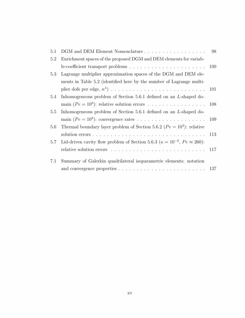
5.1 DGM and DEM Element Nomenclature . . . . . . . . . . . . . . . . . 98
5.2 Enrichment spaces of the proposed DGM and DEM elements for variab-
le-coefficient transport problems . . . . . . . . . . . . . . . . . . . . . 100
5.3 Lagrange multiplier approximation spaces of the DGM and DEM ele-
ments in Table 5.2 (identified here by the number of Lagrange multi-
plier dofs per edge, nλ) . . . . . . . . . . . . . . . . . . . . . . . . . . 101
5.4 Inhomogeneous problem of Section 5.6.1 defined on an L-shaped do-
main (Pe = 103): relative solution errors . . . . . . . . . . . . . . . . 108
5.5 Inhomogeneous problem of Section 5.6.1 defined on an L-shaped do-
main (Pe = 103): convergence rates . . . . . . . . . . . . . . . . . . . 109
5.6 Thermal boundary layer problem of Section 5.6.2 (Pe = 103): relative
solution errors . . . . . . . . . . . . . . . . . . . . . . . . . . . . . . . 113
5.7 Lid-driven cavity flow problem of Section 5.6.3 (κ = 10−2, Pe ≈ 260):
relative solution errors . . . . . . . . . . . . . . . . . . . . . . . . . . 117
7.1 Summary of Galerkin quadrilateral isoparametric elements: notation
and convergence properties . . . . . . . . . . . . . . . . . . . . . . . . 137
xv

List of Figures
2.1 Decomposition of domain Ω into elements Ωe . . . . . . . . . . . . . . 13
2.2 Illustration of stencils for first order Galerkin and DGM elements . . 30
3.1 Plots of free-space solutions cE(x; θk) to the constant-coefficient advect-
ion-diffusion equation for Case 1 (a1/κ = 20, a2/κ = 0) . . . . . . . . 37
3.2 Plots of free-space solutions cE(x; θi) to the constant-coefficient advect-
ion-diffusion equation for Case 2 (a1/κ = 20, a2/κ = 0) . . . . . . . . 39
3.3 Plots of free-space solutions cE(x; θi) to the constant-coefficient advect-
ion-diffusion equation for Case 3 (a1/κ = 20, a2/κ = 0) . . . . . . . . 41
3.4 Plots of polynomial free-space solutions to the constant-coefficient adve-
ction-diffusion equation (a1/κ = 10, a2/κ = 5) . . . . . . . . . . . . . 43
3.5 Free-space solution (3.51) for σi ∈ R . . . . . . . . . . . . . . . . . . . 47
3.6 Free-space solution (3.51) for σi ∈ C . . . . . . . . . . . . . . . . . . . 47
4.1 Graphical representation of enrichment arguments (4.3) as a circle of
radius |a| centered at a ∈ R2 . . . . . . . . . . . . . . . . . . . . . . . 50
xvi

4.2 Flow at an angle φ over Ωe = (xj, xj+1) × (yj, yj+1) . . . . . . . . . . 51
4.3 Sample unstructured mesh of 100 quadrilateral elements . . . . . . . 52
4.4 Straight edge of element Ωei oriented at angle αij . . . . . . . . . . . 53
4.5 Illustration of the sets Θc and Θλ that define the Q-8-2 element . . . 61
4.6 Plots of approximated and exact solutions of the homogeneous bound-
ary layer problem of Section 4.5.1 with φ = 0, 1,600 dofs and Pe = 103
. . . . . . . . . . . . . . . . . . . . . . . . . . . . . . . . . . . . . . . 72
4.7 Plots of approximated and exact solutions of the homogeneous bound-
ary layer problem of Section 4.5.2 with φ = π/7, ψ = 0, 1,600 dofs and
Pe = 103 . . . . . . . . . . . . . . . . . . . . . . . . . . . . . . . . . 74
4.8 Convergence rates on unstructured meshes for the homogeneous bound-
ary layer problem of Section 4.5.2 with φ = π/7, ψ = 0 and Pe = 102 75
4.9 Convergence rates for the inhomogeneous boundary layer problem of
Section 4.5.3 with φ = π/4 and Pe = 102 . . . . . . . . . . . . . . . 78
4.10 Plots of approximated and exact solutions of the inhomogeneous bound-
ary layer problem of Section 4.5.3 with φ = 0, 1,600 dofs and Pe = 103
. . . . . . . . . . . . . . . . . . . . . . . . . . . . . . . . . . . . . . . 79
4.11 L-shaped domain for the double ramp problem of Section 4.5.4 . . . . 80
4.12 Plots of approximated solutions of the double ramp problem of Section
4.5.4 with Pe = 103 and 1,200 elements . . . . . . . . . . . . . . . . 80
xvii

4.13 Nodal values of approximated solutions of the double ramp problem of
Section 4.5.4 along the line y = 0.25 with 1,200 elements . . . . . . . 82
4.14 Nodal values of approximated solutions of the double ramp problem of
Section 4.5.4 along the line y = 0.5 with 1,200 elements . . . . . . . 82
4.15 Nodal values of approximated solutions of the double ramp problem of
Section 4.5.4 along the line x = 0.5 using 1,200 elements . . . . . . . 82
4.16 Plots of approximated solutions of the double ramp problem of Section
4.5.4 along the line x = 0.95 using 1,200 elements . . . . . . . . . . . 83
5.1 Locally frozen advection fields to enable the construction of enrichment
functions as free-space solutions inside the two adjacent elements Ωe =
(xj, xj + h) × (yj, yj + h) and Ωe′ = (xj + h, xj + 2h) × (yj, yj + h) for
an example advection field a(x) = (−y, x)T . . . . . . . . . . . . . . 87
5.2 Λe,e′(θ) for the case of a quadrilateral element — extrema are marked
by circles (a1 = a2 = κ = 1) . . . . . . . . . . . . . . . . . . . . . . . 92
5.3 Illustration of the Lagrange multiplier selection procedure (Algorithm
4) for nλ = 4 . . . . . . . . . . . . . . . . . . . . . . . . . . . . . . . . 93
5.4 L-shaped domain and rotating velocity field, with curved lines indicat-
ing streamlines (Section 5.6.1) . . . . . . . . . . . . . . . . . . . . . 107
5.5 Inhomogeneous problem of Section 5.6.1 defined on an L-shaped do-
main (Pe = 103): decrease of the relative solution error with the mesh
size . . . . . . . . . . . . . . . . . . . . . . . . . . . . . . . . . . . . . 110
5.6 Thermal boundary layer problem of Section 5.6.2: domain and bound-
ary conditions . . . . . . . . . . . . . . . . . . . . . . . . . . . . . . . 111
5.7 Thermal boundary layer problem of Section 5.6.2
(
Pe = 103, h =1
30
)
:
front views of the computed solutions . . . . . . . . . . . . . . . . . . 114
5.8 Thermal boundary layer problem of Section 5.6.2
(
Pe = 103, h =1
30
)
:
rear views of the computed solutions . . . . . . . . . . . . . . . . . . 115
5.9 Domain, boundary conditions and a(x) for the lid-driven cavity flow
problem of Section 5.6.3 . . . . . . . . . . . . . . . . . . . . . . . . . 116
xviii

5.10 Components a1 and a2 of the advection field for the lid-driven cavity
flow problem of Section 5.6.3 . . . . . . . . . . . . . . . . . . . . . . . 116
5.11 Solution plots c(x) to the advection-diffusion equation for the lid-driven
cavity flow problem of Section 5.6.3 (κ = 0.005 and 40 × 40 uniform
mesh) . . . . . . . . . . . . . . . . . . . . . . . . . . . . . . . . . . . 119
5.12 Lid-driven cavity flow problem of Section 5.6.3: decrease of the relative
solution error with the mesh size (κ = 0.01, Pe ≈ 260) for the pure
DGM elements . . . . . . . . . . . . . . . . . . . . . . . . . . . . . . 120
5.13 Lid-driven cavity flow problem of Section 5.6.3: decrease of the relative
solution error with the mesh size (κ = 0.01, Pe ≈ 260) for the pure
DGM elements with higher order enrichment function . . . . . . . . . 121
5.14 Lid-driven cavity flow problem of Section 5.6.3: decrease of the relative
solution error with the mesh size (κ = 0.01, Pe ≈ 260) for the true
DEM elements . . . . . . . . . . . . . . . . . . . . . . . . . . . . . . . 122
5.15 Domain, boundary conditions and a(x) for the differentially-heated
cavity problem of Section 5.6.4 . . . . . . . . . . . . . . . . . . . . . . 122
5.16 Components a1 and a2 of the advection field for the differentially-
heated cavity problem of Section 5.6.4 . . . . . . . . . . . . . . . . . 123
5.17 Differentially-heated cavity problem of Section 5.6.4: decrease of the
relative solution error with the mesh size (κ = 2.22×10⁻⁵, Pe ≈ 1530)
for the true DEM elements . . . . . . . . . . . . . . . . . . . . . . . . 123
5.18 Differentially-heated cavity problem of Section 5.6.4: decrease of the
relative solution error with the mesh size (κ = 2.22×10⁻⁵, Pe ≈ 1530)
for the pure DGM elements . . . . . . . . . . . . . . . . . . . . . . . 124
5.19 Contours of advection-diffusion solution c(x) for the differentially-heat-
ed cavity problem of Section 5.6.4 (κ = 2.22×10⁻⁵, Pe ≈ 1530, 16×16
uniform mesh) . . . . . . . . . . . . . . . . . . . . . . . . . . . . . . . 125
5.20 Differentially-heated cavity problem of Section 5.6.4: decrease of the
relative solution error with the mesh size (κ = 2.22×10⁻⁵, Pe ≈ 1530)
for the pure DGM elements with higher order enrichment function . . 126
xix

7.1 Bilinear quadrilateral element Q1 domain and local node ordering in
the parent domain (left) and in the physical domain (right) . . . . . . 137
7.2 Shape functions of the bilinear quadrilateral Q1 element . . . . . . . 139
7.3 Azimuth and inclination angles specifying a 3D advection direction
field a ∈ R3 . . . . . . . . . . . . . . . . . . . . . . . . . . . . . . . . 142
7.4 Plots of free-space solutions to (7.40) of the form (7.66) for different
values of θi . . . . . . . . . . . . . . . . . . . . . . . . . . . . . . . . . 146
xx

Chapter 1
Introduction
The Navier-Stokes equations are the fundamental partial differential equa-
tions (PDEs) in fluid mechanics. These celebrated equations are useful in modeling
many physical phenomena of interest in modern day science and engineering appli-
cations. For example, they can help with the design of aircraft and cars, as they are
often used to model air flow around such vehicles. They can also be used to model
the weather, ocean currents, flow in a pipe or cavity, among many other things. Ob-
tained by considering the mass, momentum, and energy balances for an infinitesimal
control volume over which these principles apply, the equations describe the velocity,
pressure, temperature and density of a moving fluid. In dimensionless form, assum-
ing an incompressible Newtonian fluid, they state that the fluid velocity u ∈ Rd, for
d = 1, 2, 3 spatial dimensions, and the fluid pressure p satisfy
∂u∂t
+ u · ∇u + ∇p− 1Re
∆u = f ,
∇ · u = 0,(1.1)
where Re is a dimensionless parameter known as the Reynolds number , and f ∈ Rd
is a vector of body forces.
Because the Navier-Stokes equations are, in practice, too difficult to solve using
analytic techniques, engineers and applied mathematicians have devoted a tremen-
dous effort to developing numerical methods to solve these equations approximately
1

CHAPTER 1. INTRODUCTION 2
on a computer. The branch of fluid mechanics that uses numerical methods and al-
gorithms to solve and analyze fluid problems is known as Computational Fluid
Dynamics (CFD). Examples of some common numerical techniques in CFD, each
with its own strengths depending on the application, include spectral methods [2, 3],
finite difference methods [4], finite volume methods [5], and finite element
methods [6, 7, 8, 9, 10, 11, 12].
1.1 The finite element method (FEM) in fluid me-
chanics
The method developed in this dissertation falls in the family of numerical methods
known as finite element methods. The standard Galerkin finite element method is
based on a variational framework (or weak formulation), and a continuous, piece-
wise polynomial, Galerkin approximation. Since it was first developed in the field of
structural engineering during the 1940s, the Galerkin finite element method has been
applied to solve complicated engineering problems in a plethora of structural (e.g.,
stress analysis, buckling, vibrational analysis) as well as non-structural (e.g., heat
transfer, fluid flow, distribution of magnetic potential) applications [9]. One of the
main advantages of the FEM over other methods is its ability to handle very complex
geometries and varied boundary conditions. In addition, the theoretical framework
and approximation properties of the standard Galerkin FEM is at the present time
well established. It can be shown that the approach is optimal for the Laplace opera-
tor in the sense that it minimizes the error in the energy norm. This property assures
good performance of the computation for elliptic problems at any mesh resolution; in
other words, the method gives high coarse-mesh accuracy.
In deciding how to begin the task of building an accurate and efficient finite
element method for the Navier-Stokes equations, it is useful to write down a dis-
cretization of these equations, and remark that the advection-diffusion equation
−κ∆c(x)︸ ︷︷ ︸
diffusion
+ a · ∇c(x)︸ ︷︷ ︸
advection
= f(x), x ∈ Ω ⊂ Rd, d = 1, 2, 3, (1.2)

CHAPTER 1. INTRODUCTION 3
arises in its vector form in the linearization steps of the discretization. This ob-
servation suggests that having a method that can solve the much simpler transport
problem (1.2) accurately and efficiently is essential to fluid mechanics applications.
It is well known that the standard FEM can be inadequate when applied to (1.2)
in certain regimes. The character of the solutions of (1.2) depends on the magnitude
of a dimensionless parameter known as the the Peclet number (Pe). The Peclet
number is defined by
Pe ≡ rate of advection
rate of diffusion=lΩ maxx∈Ω ||a(x)||
κ= Re ·
Pr (thermal diffusion)
Sc (mass diffusion),
(1.3)
where Re, Pr and Sc are the Reynolds, Prandtl and Schmidt numbers respectively,
lΩ is a characteristic length scale of the domain Ω on which the problem is posed and
|| · || is some vector norm. At low values of Pe, diffusion dominates and the equation
is close to the elliptic Laplace equation. As κ → 0 (Pe → ∞), however, the exact
solutions of boundary value problems (BVPs) based on (1.2) exhibit boundary
layers, much like solutions to the Navier-Stokes equations in the high Reynolds num-
ber regime. A boundary layer is a very narrow region, typically near a physical
boundary or corner and having a width of O(Pe−1/2) [13], where the solution and its
derivatives change abruptly. In order to resolve the boundary layers that can form
using standard Galerkin piecewise polynomial finite elements, the mesh size would
have to be the same size as the ratio between the diffusion and convection [14]. In
many applications, this requirement leads to a huge number of degrees of freedom
(dofs), making the FEM not only inefficient, but sometimes simply unfeasible.
1.2 Alternatives to the classical Galerkin FEM for
advection-dominated flow problems
A number of different finite element approaches have been proposed for addressing
the challenge of solving (1.2) accurately and efficiently in the high Pe regime. These
alternatives to the standard FEM fall roughly into two categories: those based on a

CHAPTER 1. INTRODUCTION 4
modified variational formulation, and those based on a modified finite element basis.
These methods are described briefly below.
One popular class of alternatives that falls into the first category of the methods
described above is the class of so-called stabilized finite element methods . Some
examples of stabilized finite elements methods are:
• The Streamline Upwind Petrov-Galerkin (SUPG, or Streamline Dif-
fusion) method [15, 16, 6].
• The Spotted Petrov-Galerkin (SPG) [17].
• The Galerkin Least-Squares (GLS) Method [18, 19].
• The Unusual Stabilized Finite Element Method (USFEM ) [20, 21].
• The Conformal Petrov-Galerkin (CPG) method [22, 23].
The basic idea of stabilized methods is to add weighted residual terms, representing
numerical (or artificial) diffusion, to the standard weak formulation of the problem
in order to enhance stability without losing consistency. The modification to the
standard Galerkin FEM is in the variational formulation only, as stabilized methods
rely on the same polynomial basis functions as those employed in the standard FEM.
In contrast with the first category of alternatives to the standard FEM, the sec-
ond category is essentially based on non-standard finite element bases. Examples of
methods that fall into this second category of methods are:
• The method of Residual-Free Bubbles (RFB) [24, 14].
• The Partition of Unity Method (PUM ) [25, 26].
• Variational Multi-Scale Methods (VMS) [27].
• Discontinuous Galerkin Methods (DGMs) [28, 29, 30, 31, 32, 33, 34].
The former three methods are conforming methods: the finite element spaces em-
ployed in these methods are constructed so that the solution produced by the methods
is automatically continuous. In contrast, DGMs constitute a class of finite element

CHAPTER 1. INTRODUCTION 5
methods that use discontinuous functions to approximate the solution. The continu-
ity of the solution in these methods is often enforced weakly using a framework in
which appropriate numerical fluxes are defined and computed on the element bound-
aries [30, 31, 32]. DG methods can provide great advantages in solving problems with
solutions that exhibit shocks or discontinuities.
Remark 1.2.1. Although the two “classes” of methods described above are presented
as fundamentally different, there is a deep connection between some of the methods
in the former and the latter categories; cf. [35] for connections between multi-scale
formulations and stabilized FEMs, and between RFB and stabilized FEMs.
Remark 1.2.2. Note also that methods that cannot easily be placed into either one
of the two “classes” described above have been proposed. For instance:
• The Scharfetter-Gummel , or exponential-fitting, method, based on a change
of variables that transforms the advection-diffusion equation (1.2) into a ariable-
coefficient Poisson equation [36].
• Methods which use asymptotic analysis to construct approximate problems for
(1.2) in the streamline coordinates [13].
• The recently-proposed DG Petrov-Galerkin method, based on “optimal” discon-
tinuous test functions that are computed for each given BVP and guarantee
stability by effectively incorporating an upwind effect into the design of the test
function space [37].
1.3 The discontinuous enrichment method (DEM)
The method developed in this dissertation, referred to as the discontinuous en-
richment method (DEM ), falls into the second class of alternatives for the finite
element solution of (1.2) in an advection-dominated regime described above, namely
those in which non-standard finite element bases are constructed for approximating
the solution. DEM was motivated by PUM, RFB, the Finite Element Tearing and In-
terconnect (FETI) method for non-conforming domain decomposition with Lagrange

CHAPTER 1. INTRODUCTION 6
multipliers [38, 39, 40, 41], as well as the work on discontinuous Galerkin methods
(DGMs) for second-order equations [28, 29, 42, 43]. The main idea of DEM is to
enrich the standard piecewise polynomial approximations by the non-conforming and
in general non-polynomial space of free-space solutions of the homogeneous form of
the governing PDE, obtained in analytical form using standard techniques such as
separation of variables. Since these functions are related to the problem being solved,
they have a natural potential for effectively resolving sharp gradients and rapid os-
cillations when these are present in the computational domain. However, since the
functions are not required to satisfy any local boundary conditions that would ensure
inter-element continuity, the method is by construction discontinuous; inter-element
continuity in DEM is enforced weakly using Lagrange multipliers. Due to this formu-
lation, DEM can be characterized as a hybrid finite element method : an FEM
with two unknown fields, a primal field and a secondary field, with the secondary
field defined on the element interfaces [12].
1.3.1 Comparison of DEM to other methods
The discontinuous enrichment method distinguishes itself from the methods that mo-
tivated it in several ways. Whereas RFB and PUM are continuous methods, DEM
is, by construction, discontinuous. Unlike in PUM, the enrichment in DEM is per-
formed in an additive rather than multiplicative manner. Unlike in RFB, it is not
constrained to vanish at the element boundaries and therefore can propagate its
beneficial effect to the neighboring elements. Unlike in both PUM and RFB, the en-
richment in DEM leads to a discontinuous, rather than a continuous, approximation
in which the enrichment dofs can be eliminated at the element level by a static con-
densation. This reduces the computational complexity of the method, and alleviates
some of the ill-conditioning that is inherent to most enriched methods – for example,
PUM, known to suffer from severe ill-conditioning that can make the method inef-
fective in practice [44, 1, 45]. The definition of the enrichment in DEM also allows
the method to circumvent both the difficulty in approximating the global fine-scale
Green’s function of VMS [27], and the loss of global effects suffered by RFB methods

CHAPTER 1. INTRODUCTION 7
because of the requirement that the bubble functions have a vanishing trace on the
element boundaries. Although DEM can be classified as a discontinuous Galerkin
method (DGM), DEM distinguishes itself from earlier [28, 29] as well as recently
proposed [33, 34, 30, 31, 32, 37] DG methods either by its special shape functions,
which are typically non-polynomial, and/or by the Lagrange multiplier degrees of
freedom (dofs) it introduces at the element interfaces to enforce a weak inter-element
continuity of the numerical solution.
1.3.2 History of DEM and its success
DEM was first proposed approximately ten years ago by Farhat et al. [1]. Initially,
the method was developed for the Helmholz equation, Lu = −∆u − k2u = f , which
describes acoustic vibrations in a fluid medium. Since the Helmholtz operator tends to
lose ellipticity with an increasing wave number k, the Galerkin solution of Helmholtz
problems is tainted by spurious dispersion in the upper end of the low-frequency
regime, and is intractable in the medium and high frequency regimes.
Since it was first proposed, the discontinuous enrichment method has matured in
the following areas.
• Acoustic scattering (the Helmholtz equation) [46, 47].
• Wave propagation in elastic media (Navier’s equation) [48, 49].
• Fluid-structure interaction problems (coupling of Navier’s equation and the
Helmholtz equation) [50].
For these applications, the enrichment spaces consist of a superposition of plane
and/or evanescent waves. In general, it was found that DEM can achieve the same
accuracy as the p-finite element method [51] using a similar computational complexity
but with much fewer dofs. In [46], a family of three-dimensional (3D) hexahedral DEM
elements of increasing order of convergence was proposed for the solution of acoustic
scattering problems in the medium frequency regime. When compared with standard
high-order polynomial Galerkin elements of comparable convergence order, the DEM
elements achieved the same solution accuracy using, however, four to eight times

CHAPTER 1. INTRODUCTION 8
fewer dofs, and most importantly, up to 60 times less CPU time [46]. More recently,
a domain decomposition-based iterative solver for 2D and 3D acoustic scattering
problems in medium/high frequency regimes has been developed, and shown to be
superior to the classical high-order finite element method [47]. This solver was shown
to be numerically scalable with respect to the mesh size as well as the number of
enrichment functions.
An attempt to bridge the gap between numerical experimentation and mathemat-
ical analysis was made by Amara et al. [52] in the specific context of the 2D low-order
DGM element with four plane waves first proposed in [1] for solving 2D Helmholtz
problems at relatively high wave numbers. This analysis resulted in a formal proof of
the convergence of this element and revealed its theoretical order of accuracy.
1.3.3 DEM for problems in fluid mechanics
The excellent performance of DEM for acoustic scattering and wave propagation
problems is the main motivation behind the present work, in which DEM is developed
for constant and variable-coefficient advection-diffusion transport problems (1.2) in
two-dimensions (2D). The development of this method for this equation can be viewed
as a first step towards the more challenging task of building a DEM for the key
equations in fluid mechanics, namely the Navier-Stokes equations (1.1). To this effect,
the body of this dissertation is organized as follows:
• In Chapter 2, the hybrid variational formulation of a canonical 2D advection-
diffusion boundary value problem discretized by DEM is presented. The ap-
proximation spaces for the primal unknown as well as the Lagrange multiplier
approximations are defined, and an efficient implementation procedure is out-
lined.
• Chapter 3 focuses on the derivation of the enrichment field. Several families
of enrichment functions for constant- as well as variable-coefficient transport
problems are derived.
• In Chapter 4, the method is developed specifically for the equation (1.2) with

CHAPTER 1. INTRODUCTION 9
constant coefficients. Appropriate enrichment and Lagrange multiplier approx-
imation spaces are developed, and an algorithm that makes possible the sys-
tematic design and implementation of DEM elements of arbitrary orders is de-
scribed. The proposed DEM elements are evaluated on a number of challenging
constant-coefficient problems.
• In Chapter 5, attention is turned to the variable-coefficient advection-diffusion
equation (1.2). It is shown that the methodology developed specifically for
the constant-coefficient case (Chapter 4) has a natural extension to variable-
coefficient problems. It is also shown that, in the variable-coefficient scenario,
the approximation can be improved by augmenting the enrichment space with
additional families of free-space solutions to variants of the governing PDE, de-
rived in Chapter 3. The DEM elements developed in Chapter 5 are evaluated on
several challenging variable-coefficient problems possessing boundary, internal,
and crosswind layers, and compared to their Galerkin and stabilized Galerkin
counterparts.
• A summary of the method, the contributions of this dissertation, and some
discussion of possible future research directions is given in Chapter 6. The
development and numerical study of higher-order DEM elements is one of the
novel accomplishments presented in this dissertation, which distinguishes it from
prior works, namely [1, 53].
• A review of some fundamental concepts pertaining to the finite element method
can be found in the Appendix (Chapter 7).

Chapter 2
Theoretical framework of the
discontinuous enrichment method
(DEM)
In this chapter, the theoretical framework of the discontinuous enrichment meth-
od (DEM) is developed. This framework is presented in the context of a specific
boundary value problem (BVP) for the advection-diffusion equation (1.2). A brief re-
view of the classical Galerkin finite element method (FEM) and some of its stabilized
variants, based on the classical texts [6, 7, 8, 10, 54, 55], can be found in the Appendix
(Section 7.1). For additional reading on the theoretical framework of DEM, including
its formulation for other partial differential equations (PDEs) (e.g., the Helmholtz
equation), the reader is referred to the journal articles [1, 56, 57, 58, 46, 48, 50] and
the Ph.D. thesis of Oliveira [53].
10

CHAPTER 2. THEORETICAL FRAMEWORK OF DEM 11
2.1 Functional settings and notation for a canon-
ical advection-diffusion boundary value prob-
lem
Let Ω ⊂ Rd, for d = 1, 2 or 3, be an open bounded domain with a Lipschitz con-
tinuous, smooth boundary Γ ≡ ∂Ω. As a canonical example, consider the following
all-Dirichlet boundary value problem (BVP) for the advection-diffusion equation in
its strong form (S).
(S) :
Find c : Ω → R such that c ∈ H1(Ω) and
Lc ≡ −κ∆c+ a · ∇c = f in Ω,
c = g on Γ,
(2.1)
where Ω denotes the closure of Ω. The diffusivity κ is assumed to be constant and
positive, and the advection field a(x) ∈ Rd in d = 1, 2, 3 spatial directions is assumed
to be continuous over the entire domain Ω, with its ith component denoted by ai(x),
for i = 1, ..., d. In (2.1), f : Ω → R and g : Γ → R are given functions specifying
a source and Dirichlet data respectively, and H1(Ω) denotes the Sobolev space of
order one. Recall that a Sobolev space of order m is the (vector) space of functions
Hm(Ω) ≡
v ∈ L2(Ω) :∂(i+1)v
∂xi∂yj∈ L2(Ω), 0 ≤ i+ j ≤ m
, (2.2)
equipped with the inner product
(u, v)m,Ω ≡ (u, v) ≡∑
i,j
(∂(i+j)u
∂xi∂yj,∂(i+j)v
∂xi∂yj
)
0,Ω
, (2.3)
and corresponding norm
||u||m,Ω ≡ (u, u)1/2m,Ω, (2.4)

CHAPTER 2. THEORETICAL FRAMEWORK OF DEM 12
where L2(Ω) is the space of measureable, square integrable functions in Ω, equipped
with the inner product
(u, v)0,Ω ≡∫
Ω
uvdΩ. (2.5)
From this point onwards, the subscript Ω will be dropped unless the domain of inte-
gration is a subset of Ω, e.g., ||u||m,Ω ≡ ||u||m.
The process of discretizing a linear BVP in its strong form (S), e.g. (2.1), by a
finite element method (FEM) consists of the following four steps [6].
Step 1: Constructing a triangulation Th of the domain, that is, partitioning
Ω into nel disjoint element domains Ωe, each with a boundary Γe ≡ ∂Ωe
(Figure 2.1), so that
Ω = ∪nele=1Ω
e with ∩nel
e=1 Ωe = ∅. (2.6)
Step 2: Obtaining the equivalent weak (or variational) form (W ) of (2.1).
Step 3: Projecting the continuous variational problem into a finite dimensional
space through finite element shape functions used to approximate the
solution, to yield a linear system of the form
Kd = F. (2.7)
Step 4: Solving the system (2.7) for the unknown degrees of freedom (dofs)
d.
The matrix K and vector F in (2.7) are commonly referred to as the stiffness matrix
and load vector respectively.
To define the weak or variational counterpart of (S) (2.1) (Step 2 above), two
classes of functions must be characterized: the space of trial (or candidate) func-
tions and the space of test (or weighting) functions , denoted commonly by Sand V respectively. In the classical Galerkin FEM (Section 7.1.1), given a partial

CHAPTER 2. THEORETICAL FRAMEWORK OF DEM 13
Ω
Ωe
Γe
Figure 2.1: Decomposition of domain Ω into elements Ωe
differential equation (PDE) or order 2m, the spaces S and V are defined by:
S = u : u ∈ Hm(Ω), u satisfies all essential (Dirichlet) BCs of the problem, (2.8)
and
V = u : u ∈ Hm(Ω), u satisfies all homogeneous essential (Dirichlet) BCs
of the problem ,(2.9)
where Hm(Ω) is the Sobolev space defined in (2.2). In the classical Galerkin FEM,
the basic requirements on the shape functions chosen to represent the solution to
ensure convergence are:
1. [Smoothness] The shape functions must be smooth (at least C1) on each
element interior, Ωe.
2. [Continuity] The shape functions must be continuous across each element
boundary Γe.
3. [Completeness] The space of shape functions must be complete (that is,
capable of exactly representing an arbitrary linear polynomial when the nodal

CHAPTER 2. THEORETICAL FRAMEWORK OF DEM 14
degrees of freedom are assigned values in accordance with it).
A finite element method is known as a Galerkin finite element method when
S = V (modulo boundary conditions), that is, when the space of trial functions and
the space of test functions are the same. Otherwise, that is when S 6= V , the resulting
method is known as a Petrov-Galerkin finite element method .
As will become apparent in Section 2.2, the discontinuous enrichment method
(DEM) can be characterized as a hybrid finite element method , that is, a two
field mixed finite element method with the secondary unknown field defined at
the element interfaces [12]. The variational formulation of DEM will require the
introduction of some additional functional spaces, denoted by H−1/2(Γ) and H1/2(Γ).
The latter space is defined as
H1/2(Γ) = g ∈ L2(Γ) : v|Γ = g, v ∈ H1(Ω),||g||1/2 = infv∈Vg |v|1, Vg = v ∈ H1(Ω) : v|Γ = g,
(2.10)
where | · |1 denotes the following semi-norm in H1(Ω):
|v|21 ≡∫
Ω
|∇v|2dΩ. (2.11)
The space H−1/2(Γ) is the dual space of H1/2(Γ), with its norm given by
||g′||−1/2 = supg∈H1/2(Γ)
〈g′, g〉||g||1/2
= supv∈H1(Ω)
〈g′, v〉|v|1
. (2.12)
Here, 〈·, ·〉 denotes the L2(Γ) inner product over the space of measurable, square
integrable functions on the domain Γ:
〈c, v〉 =
∫
Γ
cvdΓ. (2.13)

CHAPTER 2. THEORETICAL FRAMEWORK OF DEM 15
2.2 Hybrid variational formulation of DEM
To facilitate the presentation in this section, the following notation is introduced.
The union of element interiors and element boundaries will be denoted Ω and Γ,
respectively,
Ω = ∪nel
e=1Ωe, Γ = ∪nel
e=1Γe. (2.14)
The set of element interfaces (or interior element boundaries) will be denoted by
Γint = Γ\Γ, (2.15)
and the intersection between two adjacent boundaries Γe and Γe′ will be denoted by
Γe,e′ = Γe ∪ Γe′ . (2.16)
The formulation of DEM is obtained by rewriting the strong form (S) of the
BVP (2.1) in its weak variational form . To this effect, two functional spaces are
introduced
V ≡
v ∈ L2(Ω) : v|Ωe ∈ H1(Ωe)
, (2.17)
W = ΠeΠe′<eH−1/2(Γe,e′) ×H−1/2(Γ). (2.18)
V is a space of element approximations of the solution and W is a space of Lagrange
multipliers . DEM is a Galerkin method, so that S = V ; that is, the space of test
and trial functions do not differ. Hence, from this point forward, both spaces will be
denoted by V (2.17).
A key feature of DEM is that the space of element approximations — that is, the
discrete analog of V (2.17) — is allowed to be discontinuous across element interfaces.
That is, the second property of the three shape function criteria enumerated in Section
2.1 (Smoothness, Continuity and Completeness) can be violated. Since it is typically
desired that the numerical solution remain continuous across the element interfaces
in some sense, the following inter-element continuity constraint is added to the BVP

CHAPTER 2. THEORETICAL FRAMEWORK OF DEM 16
(2.1):
[[c(x)]] ≡∣∣∣∣
lim[x∈Ωe]→Γe,e
′c(x) − lim
[x∈Ωe′]→Γe,e
′c(x)
∣∣∣∣= 0, x ∈ Γint. (2.19)
The constraint (2.19) may be enforced weakly using Lagrange multipliers or by the
penalty method. In DEM, the former weak enforcement is adopted – that is, (2.19)
is enforced weakly using Lagrange multipliers belonging to the space W (2.18).
The weak form of the BVP (2.1) is obtained first by multiplying the first equation
in (2.1) by a test function v ∈ V and integrating the diffusion term by parts:
∫
Ω
(−κ∆c+ a · ∇c)vdΩ = −κ∫
Γ
(∇c · n︸ ︷︷ ︸
≡Lbc)vdΓ +
∫
Ω
(κ∇c · ∇v + a · ∇cv)dΩ. (2.20)
Here, Lb is the boundary operator corresponding to L. Constraining the solution to
remain continuous across the element interfaces, that is, the addition of the constraint
(2.19), leads to the following weak hybrid variational formulation
(W ) :
Find (c, λ) ∈ V ×W such that
a(v, c) + b(λ, v) = r(v) ∀v ∈ V ,b(µ, c) = −rd(µ) ∀µ ∈ W ,
(2.21)
where a(·, ·) and b(·, ·) are bilinear forms on V × V and W ×V respectively. They
are given by
a(v, c) ≡ (κ∇v + va,∇c)Ω =
∫
Ω
(κ∇v · ∇c+ va · ∇c)dΩ, (2.22)
b(λ, v) ≡∑
e
∑
e′<e
∫
Γe,e′λ(ve′ − ve)dΓ +
∫
Γ
λv dΓ, (2.23)
In (2.21), r(v) and rd(µ) (d for “Dirichlet”) are the following linear forms
r(v) ≡ (f, v) =
∫
Ω
fvdΩ, (2.24)
rd(µ) ≡ 〈µ, g〉 =
∫
Γ
µgdΓ. (2.25)

CHAPTER 2. THEORETICAL FRAMEWORK OF DEM 17
In (2.22) and (2.24), (·, ·) denotes the usual L2 inner product over Ω (2.5) and 〈·, ·〉denotes the usual L2 inner product over Γ (2.13); in (2.23), ve ≡ v|Ωe . Note that the
bilinear form a(·, ·) in (2.22) is not symmetric(a(v, c) 6= a(c, v)
)for the advection-
diffusion operator due to the presence of the first order advection term.
Remark 2.2.1. The variational form (2.21) is not unique. Assuming a is divergence-
free (or incompressible), that is ∇ · a = 0, the following identity holds:
a · ∇c = ∇ · (ac), (2.26)
so that
a · ∇c = αa · ∇c+ (1 − α)∇ · (ac), (2.27)
for α ∈ [0, 1]. Substituting (2.27) into the first equation in (2.1), multiplying this
equation by a test function v ∈ V, and performing an integration by parts not only on
the diffusion term but also the advection term (1 − α)∇ · (ac) gives:
∫
Ω(−κ∆c+ a · ∇c)vdΩ =
∫
Γ[(1 − α)a · nc− κ∇c · n] vdΓ
+
∫
Ω
[α(a · ∇c)v − (1 − α)(a · ∇v)c+ κ∇c · ∇v] dΩ︸ ︷︷ ︸
aα(v,c)
.
(2.28)
Comparing (2.28) with (2.20), the reader may observe that the procedure just outlined
has resulted in a modified bilinear form aα(·, ·), defined in (2.28). The form (2.22) can
be recovered from (2.28) by setting α = 1, and is commonly referred to as the con-
vective form . When α = 12, the form (2.28) is referred to as the skew-symmetric
form [59], due to the property that
a(v, c) ≡ 1
2
∫
Ω
[(a · ∇c)v − (a · ∇v)c] dΩ (2.29)
is skew-symmetric, that is a(c, v) = −a(v, c).

CHAPTER 2. THEORETICAL FRAMEWORK OF DEM 18
Remark 2.2.2. The weak form (W ) (2.21) is equivalent to a constrained minimiza-
tion problem, namely
minimize
s.t.
8
>
<
>
:
v ∈ V,
[[v]] = 0, on Γint,
v = g on Γ
J(v), (2.30)
where
J(v) ≡ 1
2a1/2(v, v) − r(v) =
κ
2(∇v,∇v) − r(v). (2.31)
(2.30) can be transformed into an unconstrained minimization problem [53, 1] through
the definition of the Lagrangian :
L(v, µ) ≡ J(v) + b(µ, v) + rd(µ), (2.32)
so that (2.30) is equivalent to
minv∈V
maxµ∈W
L(v, µ). (2.33)
The saddle point equations for (2.33) give rise to the weak formulation (2.21) as well
as the Euler-Lagrange equations (2.34).
Denoting the jump at an element boundary by [[·]], the Euler-Lagrange equa-
tions corresponding to (W ) are
Lc ≡ −κ∆c+ a · ∇c = f in Ω,
[[c]] = 0 on Γint,
c = g on Γ,
λ = Lbc = ∇c · n on Γ.
(2.34)
The last equation in (2.34) provides an interpretation of the Lagrange multiplier field:
since for this problem the boundary operator Lb corresponding to L is the normal
derivative of the solution(see (2.20)
), the Lagrange multiplier field is the normal
derivative of the solution to the BVP (2.1) on the element interfaces.

CHAPTER 2. THEORETICAL FRAMEWORK OF DEM 19
2.3 Approximation spaces in DEM
The finite-dimensional analog of the hybrid DEM formulation (2.21) is obtained by
selecting finite dimensional solution spaces for the primal unknown and dual Lagrange
multiplier fields, denoted respectively by
Vh ⊂ V , Wh ⊂ W , (2.35)
where h denotes the generic size of a typical element Ωe. Once the approximation
spaces Vh and Wh are constructed, an approximate solution (ch, λh) ∈ (Vh,Wh) of
the Galerkin problem corresponding to (2.21) is sought.
2.3.1 The primal approximation space Vh
In the classical Galerkin finite element method, the trial functions are continuous
piecewise polynomials within each element Ωe — that is, ch = cP with
cP ∈ VP ⊂ Pn(x, y) ⊂ H1(Ω), (2.36)
where
Pn(x, y) ≡
p ∈ H1(Ωe) : p(x, y) =n∑
i=0
aixiyi, (x, y) ∈ Ωe, ai ∈ R, n ∈ N
, (2.37)
is a polynomial interpolation space satisfying the three properties enumerated in
Section 2.1 (Smoothness, Continuity and Completeness). A popular class of shape
functions that satisfies these properties is the set of isoparametric shape func-
tions (Chapter 3 of [6]). These shape functions are reviewed briefly in Section 7.1.1
of the Appendix.
In DEM [1, 56, 57, 58, 46, 48, 50], the primal unknown ch which defines the
approximation space Vh has one of the following two forms
ch =
cP + cE, if f 6= 0 in (2.1) (true DEM element),
cE, if f ≡ 0 in (2.1) (pure DGM element).(2.38)

CHAPTER 2. THEORETICAL FRAMEWORK OF DEM 20
cP ∈ VP ⊂ H1(Ω) are standard, continuous, piecewise polynomial finite element
shape functions (2.36), and cE ∈ VE are the so-called enrichment functions .
The weak enforcement of continuity through the constraint (2.19) leaves much
flexibility as to the design of the space VE. At the heart of DEM is the idea that VE
should be designed in a way that incorporates some information about the particular
BVP being solved. To this effect, VE is defined in DEM as the set of free-space solu-
tions of the homogeneous PDE to be solved which are not represented in VP (so as to
avoid linear dependencies with functions already represented in VP ). Mathematically,
VE ⊂LcE = 0 in R
d, (2.39)
for a generic linear PDE Lc = f in d = 1, 2, 3 spatial dimensions.
As (2.38) suggests, two varieties of DEM can be defined: a true or “full” DEM,
and an enrichment-only DEM referred to in the remainder of this dissertation as
“DGM” (for discontinuous Galerkin method). In variational multiscale (VMS)
[27] terminology, the splitting of the approximation into polynomials and enrichment
functions, as done in the first line of (2.38), can be viewed as a decomposition of the
numerical solution into coarse (polynomial) and fine (enrichment) scales. Elements
for which the solution space Vh is constructed as a direct sum of VP and VE are
termed “full” or true DEM elements. The general rule of thumb is to employ these
elements when solving inhomogeneous problems, as the enrichment field defined by
(2.39) is not guaranteed to span the particular solutions to these PDEs. If the PDE
to be solved is homogeneous to begin with, however, the enrichment field (2.39)
may entirely capture the solution to the problem, rather than merely enhance the
polynomial field. This motivates the construction of so-called pure DGM elements(second line of (2.38)
), for which the contribution of the standard polynomial field
VP is dropped from Vh, resulting in improved computational efficiency without a loss
of accuracy (Section 2.4.3).
The careful reader may observe that in defining the enrichment space VE as in
(2.39), it has been assumed that the homogeneous free-space solutions to Lc = 0
are available in closed analytical form for the given operator L. In general, it is

CHAPTER 2. THEORETICAL FRAMEWORK OF DEM 21
possible to obtain these solutions analytically primarily for linear PDEs with constant
coefficients. As discussed in detail in Chapter 5, since the enrichment functions in
DEM are to be employed at the element level, it is natural to use the solutions of the
constant-coefficient version of the PDE of interest — that is, use a fixed value of the
advection field a(x) ≡ a in (1.2) inside each element — to define the enrichment field
VE in the more general variable-coefficient context.
2.3.2 Babuska-Brezzi inf-sup condition
As DEM is a hybrid method, care must be taken to design the space Wh such that the
well known Babuska-Brezzi inf-sup condition [12, 55, 60], a necessary condition
for ensuring a non-singular global interface problem from the discrete form of (2.21),
is upheld. This condition is reviewed briefly in this section.
Recall the bilinear forms a : V × V and b : V × W defined in (2.22) and (2.23)
respectively. Let A : V → V and B : W → V denote linear bounded operators
associated with these forms, that is
a(v, c) = (v, Ac)V×V ,
b(λ, v) = (λ,Bv)W×W = (BTλ, v)V×V ,(2.40)
where (·, ·)V×V and (·, ·)W×W denote the inner products on V ×V and W×W respec-
tively. It is well known [54] that
Ac+BTλ = f
Bc = 0,(2.41)
has a unique solution, that is, is a well-posed problem, if
(i) The bilinear form a(·, ·) is coercive on kerB = v ∈ V : b(µ, v) = 0,∀µ ∈ W.
(ii) The map B is surjective.
If B has a closed range, typically (ii) can be replaced with the condition that BT is
injective. The condition (ii) is commonly referred to as the Babuska-Brezzi, or inf-sup
condition.

CHAPTER 2. THEORETICAL FRAMEWORK OF DEM 22
To extend this condition to the discrete problem, let Ah : Vh → Vh and Bh :
Wh → Vh denote the discrete versions of the operators defined in (2.40). Then, the
following theorem describes the existence and uniqueness of solutions of the discrete
version of the variational problem (2.21) (Prop. II.2.1 in [12]).
Theorem 2.3.1. If there exists vh ∈ Vh such that b(µh, vh) = −rd(µh) for any
µh ∈ Wh and there exist positive constants α and γ independent of h such that
infch∈KerBh
supvh∈KerBh
a(vh, ch)
||ch||V ||vh||V≥ α, (2.42)
and
infµh∈Wh
supvh∈Vh
b(µh, vh)
||vh||V ||µh||W\KerBT
≥ γ, (2.43)
then the discrete analog of (2.21) has a unique solution (ch, λh) ∈ Vh ×Wh\KerBTh ,
whereKerBh ≡ vh ∈ Vh : b(µh, vh) = 0,∀µh ∈ Wh,KerBT
h ≡ µh ∈ Wh : b(µh, vh) = 0,∀vh ∈ Vh.(2.44)
Moreover,
||c− ch||V + ||λ− λh||Wh\KerBTh≤ C
(
infvh∈Vh
||c− vh||V + infµh∈Wh
||λ− µh||W)
, (2.45)
for some constant C ∈ R.
Condition (2.43) is the discrete version of the as the Babuska-Brezzi or inf-sup
condition. Care must be taken to design the spaces Vh and Wh such that this con-
dition is upheld, as the failure of the condition can put into jeopardy the solvability
of the system arising from the discrete form of (2.21). An extensive survey for dis-
cretizing a Lagrange multiplier field of a form similar to that considered herein can
be found in Section 3.3 of [12]. Most, if not all, of these established techniques and
theoretical results are for standard polynomial approximations of the solution ch. Ex-
tending these ideas, namely designing the approximation spaces such that it can be
proven a priori that the bilinear form b(·, ·) satisfies the condition (2.43), to the typ-
ically non-polynomial approximations cE employed in DEM is not a straightfoward

CHAPTER 2. THEORETICAL FRAMEWORK OF DEM 23
task. Some progress has been made by Amara et al. in the context of low-order
DEM elements for the Helmholz equation and plane wave enrichment functions [52],
but the task of showing that (2.42) holds for the advection-diffusion DEM elements
developed in this dissertation remains an open problem at the present time.
The elements proposed in this dissertation are developed to satisfy an inf-sup
condition for the discrete, finite dimensional problem of (2.21). This algebraic inf-
sup condition is a necessary condition for (2.43) to hold. By inspection, assuming
without loss of generality that g = 0, it is straightforward to see that this (global)
system will have the form:
(
A BT
B 0
)(
ch
λh
)
=
(
f
0
)
, (2.46)
where ch ∈ Rn and λh ∈ R
p are vectors containing the primal unknown and Lagrange
multiplier unknown dofs respectively, so that the matrices A and B are n × n and
p× n respectively, and f ∈ Rn, for n, p ∈ N are the number of enrichment equations
and the number of Lagrange multiplier equations, respectively. It is possible to derive
conditions on Vh and Wh for this discrete condition to hold by examining the matrix
form of the problem arising from the discretization of (2.21). The system (2.46) has
no solution if is it over-determined (and inconsistent). The matrix A represents the
global stiffness matrix and must be non-singular by construction. It is straightforward
to see, from basic linear algebra, that, assuming A is non-singular, (2.46) is overde-
termined if p > n. The outcome of this condition puts the following bound on the
dimension of the Lagrange multiplier approximation space Wh given an enrichment
space VE of nE linearly independent basis functions:
# of enrichment
equations
≥
# Lagrange multiplier
constraint equations
. (2.47)
Assuming a mesh of nel = n2 quadrilateral elements, with nE enrichment functions
in each element, and nλ Lagrange multiplier approximations per edge, the left hand
side of (2.47) is nEn2 and the right hand side is 2n(n + 1)nλ, so that (2.47) implies

CHAPTER 2. THEORETICAL FRAMEWORK OF DEM 24
that
nEn2 ≥ 2n(n+ 1)nλ ≈ 2n2nλ. (2.48)
It follows from (2.48) that the asymptotic bound on the number of Lagrange multi-
pliers per edge (nλ) is given by
nλ ≤ nE
2, (2.49)
almost everywhere in the mesh.
In Section 2.3.3, a space of Lagrange multiplier approximations for the 2D advection-
diffusion equation that is related to the normal derivatives of the enrichment functions
cE on the element edges in a well-defined way is constructed, taking care to limit its
cardinality to avoid violating the bound (2.49).
Remark 2.3.2. The condition (2.49) is a necessary, but in general not a sufficient,
condition for ensuring that a non-singular global interface problem arises in the ap-
plication of the DEM on a mesh of quadrilateral elements. In practice, fewer than
nλ = nE
2Lagrange multipliers per edge will be used. Numerical tests (Sections 4.5 and
5.6) show that the general rule of thumb is to limit
nλ =
⌊nE
4
⌋
, (2.50)
where bxc ≡ maxn ∈ Z|n ≤ x for any x ∈ R.
Remark 2.3.3. Another algebraic version of the inf-sup condition (2.43) is kerBT =
0. If this holds, (2.46) will be an under-determined system with an infinite number
of solutions. This can result in the presence of spurious modes in the computation
(Chapter 4 of [54]).
2.3.3 The dual space of Lagrange multiplier approximations
Wh
An expression for the Lagrange multiplier approximations constituting the space Wh
given an approximation space Vh can be derived from the weak form (2.21) using some

CHAPTER 2. THEORETICAL FRAMEWORK OF DEM 25
variational calculus. Applying the bilinear form a(·, ·) defined in (2.22) to c, v,∈ Vand integrating by parts the
∫
Ω∇v · ∇cdΩ term gives
a(c, v) =
∫
Ω
(−κ∆c+a·∇c)vdΩ+
∫
Γ
κ∇c·nvdΓ+∑
e
∑
e′
∫
Γe,e′κ(∇ce·neve+∇ce′ ·ne′ve′)dΓ,
(2.51)
where ne is the outward unit normal to Γe (and similarly for ne′ and Γe′). Substituting
(2.51) into the first equation in the weak form (2.21) leads to
λ = ∇ce · ne = −∇ce′ · ne′ on Γe,e′ , (2.52)
and
λ = −∇c · n on Γ, (2.53)
if a Dirichlet boundary condition is to be enforced on Γ. (2.52) suggests choosing
λh ≈ ∇cEe · ne = −∇cEe′ · ne′ on Γe,e′ , (2.54)
as a good approximation of the Lagrange multiplier on an edge Γe,e′ ; that is, defining
the space Wh to consist of the approximate normal derivatives of cE on the element
edges – but being careful not to violate the bound (2.49) arising from the discrete form
of the Babuska-Brezzi inf-sup condition (2.43). In practice, the number of Lagrange
multiplier approximations allowed per edge given nE enrichment functions will be set
according to the rule of thumb (2.50) (Remark 2.3.2).
2.4 Galerkin formulation and implementation of
DEM
Assuming the more general case of the full DEM and substituting the approximation
ch (the first row of (2.38)) into the weak form (2.21) results in the following discrete

CHAPTER 2. THEORETICAL FRAMEWORK OF DEM 26
Galerkin problem
(G) :
Find (ch, λh) ∈ Vh ×Wh such that
a(vP , cP ) + a(vP , cE) + b(λh, vP ) = r(vP ),
a(vE, cP ) + a(vE, cE) + b(λh, vE) = r(vE),
b(µh, cP ) + b(µh, cE) = −rd(µh),
holds ∀(vh, µh) ∈ Vh ×Wh.
(2.55)
The above system of Galerkin equations (G) gives rise to the element matrix equation
kPP kPE kPC
kEP kEE kEC
kCP kCE 0
︸ ︷︷ ︸
≡ke
cP
cE
λh
=
rP
rE
rC
︸ ︷︷ ︸
≡re
, (2.56)
where cP , cE and λh are vectors containing the local dofs cP , cE and λh, respectively.
The superscript e designates the element domain and the superscript C designates
the continuity constraints enforced by the Lagrange multipliers. The correspondence
between the matrices and the Galerkin equations is obtained by comparing (2.55) and
(2.56), and is summarized in Table 2.1.
Note that kEP 6= kPET as a result of the asymmetry of the bilinear form a(·, ·)for the advection-diffusion operator. In the case of a pure DGM implementation,
kPP, kPE, kPC, kEP, kCP, rP = ∅ (that is, they are empty and can be omitted)
and therefore the three-by-three block system (2.56) reduces to a two-by-two block
system, namely(
kEE kEC
kCE 0
)(
cE
λh
)
=
(
rE
rC
)
. (2.57)
2.4.1 Integration of a(·, cE)
If the enrichment field VE is comprised of free-space solutions to (2.1), the volume
integrals appearing in the bilinear forms a(·, cE) (2.22) can be converted to integrals

CHAPTER 2. THEORETICAL FRAMEWORK OF DEM 27
Table 2.1: Correspondence between the local matrices in (2.56) and the bilinear/linearforms in (2.55)
Matrix Galerkin TermkPP a(vP , cP )kPE a(vP , cE)kPC 〈vP , λh〉Γint
kEP a(vE, cP )kEE a(vE, cE)kEC 〈cE, λh〉Γint
kCP 〈µh, cP 〉Γint
kCE 〈µh, cE〉Γint
rP r(cP )rE r(cE)rC −rd(λ
h)
over the edges of each element. That is, if LcE = 0, then, for vh ∈ Vh:
0 =
∫
Ωe[a · ∇cE − κ∆cE]vhdΩ =
∫
Ωe[a · ∇cEvh + κ∇cE∇vh]dΩ
︸ ︷︷ ︸
a(vh,cE)Ωe
−κ∫
Γe∇cE · nvhdΓ.
(2.58)
Rearranging (2.58) gives
a(vh, cE)Ωe = κ
∫
Γe∇cE · nvhdΓ. (2.59)
Thus, integration in element domains can be replaced by integration along element
boundaries. It follows that, from Table 2.1, in the case of a homogeneous constant-
coefficient BVP and a pure DGM element, no volume integrals need to be computed
at all.
2.4.2 Static condensation at the element level
Due to the discontinuous nature of VE, cE can be eliminated at the element level by
a static condensation . For a full DEM element, taking the Schur complement of
the second equation in (2.56) and substituting this expression into the first and third

CHAPTER 2. THEORETICAL FRAMEWORK OF DEM 28
equations leads to the following (local) statically-condensed system
(
kPP kPC
kCP kCC
)
︸ ︷︷ ︸
≡ke
(
cP
λh
)
=
(
rP
rC
)
︸ ︷︷ ︸
≡re
, (2.60)
where
kPP = kPP − kPE(kEE)−1kEP, (2.61)
kPC = kPC − kPE(kEE)−1kEC, (2.62)
kCP = kCP − kCE(kEE)−1kEP, (2.63)
kCC = −kCE(kEE)−1kEC, (2.64)
and
rP = rP − kPE(kEE)−1rE, (2.65)
rC = rC − kCE(kEE)−1rE. (2.66)
In the case of a DGM element, there is no polynomial field and therefore kPP,
kPC, kCP, rP = ∅. Since kCC reduces to kCC = −kCE(kEE)−1kEC, the statically-
condensed system for a DGM element is therefore simply
−kCE(kEE)−1kEC
︸ ︷︷ ︸
=ke=kCC
λh = rC − kCE(kEE)−1rE
︸ ︷︷ ︸
=re=rC
. (2.67)
Equations (2.60) and (2.67) give rise either to a cP -λh formulation for the full
DEM approximation, or simply to a λh-formulation for its DGM variant. The global
condensed system is obtained from an assembly of the statically-condensed element
arrays ke and re. From this system, the Lagrange multiplier dofs, and, when ap-
plicable, the polynomial dofs, are solved for, after which the enrichment dofs are
computed by means of a post-processing step local to each element. The key steps of
this implementation are summarized in Algorithm 1.

CHAPTER 2. THEORETICAL FRAMEWORK OF DEM 29
Algorithm 1 Element-level static condensation algorithm
Compute the entries of the element matrices in (2.56) (Table 2.1).Compute the local Schur complements in (2.61)-(2.66).Assemble the global interface problem (2.60).Solve for the vector λh (and the vector cP, if applicable, i.e., in the case of the fullDEM).for each element Ωe, e = 1, . . . , nel do
Compute cE as a post-processing step within Ωe as follows
kEEcE = rE − kEPcP − kECλh, (2.68)
(with kEP = ∅ in the case of a DGM element.)end for
2.4.3 Computational complexity
An important remark at this point in the discussion is that the cost of solving the
global interface problem (2.60) is not directly determined by the dimension of VE.
Instead, it depends on the total number of Lagrange multiplier dofs — that is, on
dimWh. This property is a result of the element-level static condensation which is
enabled by the discontinuous nature of the approximation of the solution (Section
2.4.2). As discussed in Section 2.3.2, the Babuska-Brezzi inf-sup condition must be
satisfied to ensure that the global interface problem is non-singular. In particular, by
(2.49), the dimension of the space Wh will necessarily be less than the dimension of
the primal unknown space VE. Note that this property brings a major computational
advantage over PUM [25, 26].
Table 2.2 summarizes the computational complexities of some DGM and DEM el-
ements having nλ Lagrange multipliers per edge, compared to their standard quadri-
lateral Galerkin FEM counterparts, denoted by Qn (described in Section 7.1.1 of the
Appendix), for n = 1, 2, 3, 4. The table reports also the elements’ stencil widths
assuming an n × n uniform mesh of quadrilateral elements. The stencil width is
essentially the maximum number of non-zero entries in the rows of the global system
matrix that comes from assembling the local matrices (2.60). Figure 2.2 illustrates the
stencils of a first order Galerkin quadrilateral element, referred to as Q1, and a pure
DGM element having nλ = 1 Lagrange multiplier approximations per element edge.

CHAPTER 2. THEORETICAL FRAMEWORK OF DEM 30
The reader may observe by examining Table 2.2 that the stencil width of a DGM
element with nλ Lagrange multipliers per edge is smaller than that of a Galerkin
element Qnλ element; however the pure DGM element contains nel more total dofs.
As computational complexity depends on the total number of dofs and the sparsity
pattern of the system matrices (measured by the finite element stencil width), it can
be reasonably assumed that the computational complexities of a pure DGM element
with nλ Lagrange multipliers is roughly comparable to the computational complexity
of a Galerkin Qnλ element.
(a) Q1 (b) DGM element with nλ = 1
Figure 2.2: Illustration of stencils for first order Galerkin and DGM elements
2.5 Linear least squares “qualifying test” for en-
richment functions
The enrichment in DEM, defined as the set of free-space solutions to the governing
constant-coefficient homogeneous PDE, is intuitively appealing, as these solutions are
related to the operator governing the problem to be solved. Unlike the standard finite
element polynomial interpolants, however, it is unclear what can be said about the
completeness property of a proposed enrichment space (Property 3 in Section 2.1).
The following question arises: how capable are the enrichment functions comprising
VE of representing the exact (or reference) solution to a particular BVP?
Given an exact (or reference) solution to a BVP, the answer to this question can be
studied a posteriori by formulating and solving the following linear least squares

CHAPTER 2. THEORETICAL FRAMEWORK OF DEM 31
Table 2.2: Computational complexity of some DGM, DEM and standard Galerkinelements (assuming a discretization into nel quadrilateral elements)
Element Asymptotic # of dofsStencil width for
uniform n× n mesh
Galerkin
Q1 nel 9Q2 3nel 21Q3 5nel 33Q4 7nel 45
DGM with
nλ = 1 2nel 7nλ = 2 4nel 14nλ = 3 6nel 21nλ = 4 8nel 28
DEM with
nλ = 1 3nel 21nλ = 2 5nel 33nλ = 3 7nel 45nλ = 4 9nel 57
(LLS) optimization problem in each element Ωe
minaei∈R
∣∣∣∣∣∣∣∣∣∣
∣∣∣∣∣∣∣∣∣∣
nE∑
i=1
aei c
E,ei (x) − ceref(x)
︸ ︷︷ ︸
r≡Ay−b
∣∣∣∣∣∣∣∣∣∣
∣∣∣∣∣∣∣∣∣∣2
, x ∈ R2. (2.69)
Here, ceref is a reference (or exact) solution to a particular BVP in element Ωe, the
aei are the computed enrichment degrees of freedom, and cE,e
i (x) are the enrichment
functions inside that element. If the norm in (2.69) is taken to be the discrete vector
two-norm, the (2.69) can be solved using the singular value decomposition (SVD). In
particular, if A = UΣVT is the SVD of the matrix A defined in (2.69), then this

CHAPTER 2. THEORETICAL FRAMEWORK OF DEM 32
argument can be written as:
||Ay − b||2 = ||UΣVTy − b||2= ||U[ΣVTy − UTb]||2= ||ΣVTy
︸︷︷︸
≡z
−UTb︸︷︷︸
≡b′
||2.(2.70)
From (2.70), it is straightforward to see that that the solution to (2.69) is y = Vz
where, letting zi and b′i denote the ith entry of the vectors z and b respectively, and
letting σi denote the ith singular value of A,
zi =b′iσi
, i = 1, ..., r ≡ rank(Σ). (2.71)
The minimum value of the residual in (2.69) is
||r||2 =n∑
i=r+1
b′i, (2.72)
where n is the number of points at which x is sampled in element Ωe.
The solution to (2.69) gives some insight into how well the enrichment functions
employed in element Ωe are capable of representing the reference solution in that
element. Provided a reference solution (or some solution believed to be similar in
character to the exact solution to a BVP) is available, it can be worthwhile, especially
for variable-coefficient problems, to perform the test (2.69) for a proposed enrichment
basis of functions cEi (x) prior to implementing DEM in order to determine if the
proposed enrichment functions are capable of representing the reference solution to
the problem better than the standard Galerkin polynomial shape functions.
Remark 2.5.1. The LLS test described here is used to provide justification for omit-
ting certain classes of free-space solutions (derived in Chapter 3) – namely functions
with behavior deemed uncharacteristic of the solution to the boundary value problems
considered herein – from the design of the space VE.

Chapter 3
Free-space solutions to the 2D
advection-diffusion equation
In this chapter, several families of free-space solutions to the advection-diffusion equa-
tion (1.2) in two-dimensions (2D) are derived. These functions will be used to define
the enrichment spaces VE of various DGM and DEM elements in subsequent chapters.
3.1 Free-space solutions to the 2D advection-diff-
usion equation with constant a ∈ R2
First, some free-space solutions to the constant-coefficient version of (1.2) are derived.
These solutions fall into three families:
1. Functions that are exponential in both the x- and y-coordinate directions.
2. Functions that are exponential in one variable and trigonometric in the other.
3. Polynomial functions.
The first two families are derived by the standard PDE solution technique known as
separation of variables (Section 3.1.1); the third is derived by assuming a finite
power series solution and solving a system of equations for the unknown coefficients
in this series (Section 3.1.2).
33

CHAPTER 3. FREE-SPACE SOLUTIONS TO 2D ADVECTION-DIFFUSION 34
3.1.1 Separation of variables solutions
Suppose aT = (a1, a2) ∈ R2, and assume the following functional form for the
solution to LcE = −κ∆cE + a · ∇cE = 0:
cE(x, y) = F (x)G(y). (3.1)
Here, F,G : R → R are some C2(R) functions that will be determined such that
LcE = 0 is satisfied. Substituting (3.1) into (1.2) implies
a1
κF ′(x) − F ′′(x)
F (x)=G′′(y) − a2
κG′(y)
G(y)≡ k ∈ R. (3.2)
(3.2) can be decomposed into the following two ordinary differential equations (ODEs)
for the functions unknown F (x) and G(y), to be determined
F ′′(x) − a1
κF ′(x) + kF (x) = 0,
G′′(y) − a2
κG′(y) − kG(y) = 0.
(3.3)
The solutions to (3.3) are spanFk(x) and spanGk(y), where
Fk(x) =
exp
a1x2κ
±√
a21−4kκ2
2κx
if k ≤ a21
4κ2 ,
exp
a1x2κ
± i√
−a21+4kκ2
2κx
if k >a21
4κ2 ,(3.4)
Gk(y) =
exp
a2y2κ
±√
a22+4kκ2
2κy
if k ≥ − a22
4κ2 ,
exp
a2y2κ
± i√
−a22−4kκ2
2κy
if k < − a22
4κ2 ,(3.5)
and i ≡√−1. The form of the solution (3.1) thus depends on the value of the
separation of variables constant k relative to the given advection velocities a1 and
a2. The expressions (3.4) and (3.5) imply that the solution can take on one of three
forms, summarized in Table 3.1. In the first case, the enrichment function cE is a
rapidly rising or falling exponential in both the x- and y-coordinate directions. In the

CHAPTER 3. FREE-SPACE SOLUTIONS TO 2D ADVECTION-DIFFUSION 35
second and third cases, the enrichment is oscillatory in one direction.
Table 3.1: Forms of the free-space solution cE to a · ∇cE − κ∆cE = 0
k Fk(x) Gk(y)
∈[
− a22
4κ2 ,a21
4κ2
]
Exponential Exponential
∈(
−∞,− a22
4κ2
)
Exponential Trigonometric
∈(
a21
4κ2 ,∞)
Trigonometric Exponential
While the expressions in (3.4)–(3.5) are correct mathematically and cEk (x, y) =
Fk(x)Gk(y) solves LcEk = 0 for any choice of k ∈ R, there is a practical issue that is
worth addressing: it is unclear how the parameter k should be selected to generate
a particular enrichment basis, since this parameter can take on any real value from
−∞ to ∞. To this effect, it is recalled here that when DEM was tailored to the 2D
Helmholtz equation −∆c − k2c = 0 in [56], the enrichment space VE consisted of a
superposition of two-dimensional plane waves cE|Ωe = eikx cos θpeiky sin θp (where, again,
i ≡√−1), propagating in directions θp ∈ [0, 2π). The fact that the basis functions
for the Helmholtz equation were specified by an angle proved to be very convenient
as it made possible the systematic design of DEM elements of arbitrary orders: to
design an element of order nE, one simply selected nE plane waves propagating in nE
different directions. Guided by DEM for the Helmholtz equation, an expression for
cE is sought after here in which the constant k is replaced by some angle parameter.
The derivation of a parametrization of this sort is detailed below.
Case 1: Free-space solutions that are exponential in x and y
Suppose k ∈[
− a22
4κ2 ,a21
4κ2
]
. Defining µ1, µ2 ∈ R by
µ21 ≡ a2
2 + 4kκ2, µ22 ≡ a2
1 − 4kκ2, (3.6)

CHAPTER 3. FREE-SPACE SOLUTIONS TO 2D ADVECTION-DIFFUSION 36
the following identity holds
µ21 + µ2
2 = a21 + a2
2 ≡ |a|2. (3.7)
Relation (3.7) motivates the following definition
µ1 ≡ |a| cos θk, µ2 ≡ |a| sin θk, (3.8)
for some angle parameter θk ∈ [0, 2π). Given this parameterization, equations (3.4)
and (3.5) can be rewritten in terms of µ1 and µ2 as
Fk(x) = expa1x
2κ± µ1
2κx
, Gk(y) = expa2y
2κ± µ2
2κy
, (3.9)
so that
cE(x; θk) = span
e
“
a1±|a| cos θk2κ
”
xe
“
a2±|a| sin θk2κ
”
y
. (3.10)
The natural interpretation of the angles θk is that they are flow directions. Each
angle θk that appears in (3.10) specifies a function that “slopes” — that is, exhibits
a sharp gradient — in some direction in R2. Figure 3.1 shows plots of the enrichment
basis functions for several angles θk.
Remark 3.1.1. The parametrization of the exponential free-space solutions (3.10)
has a natural extension to the constant-coefficient advection-diffusion equation (1.2)
in three dimensions (3D) (Section 7.2 of the Appendix).
Case 2: Free-space solutions that are exponential in x and trigonometric
in y
Suppose k < − a22
4κ2 . It follows that a21 − 4kκ2 > 0 and a2
2 + 4kκ2 < 0. Defining µ3 and
µ4 as follows
µ23 ≡ a2
1 − 4kκ2 > 0, µ24 ≡ −a2
2 − 4kκ2 > 0, (3.11)
the following identity holds
µ23 − µ2
4 = a21 + a2
2 = |a|2. (3.12)

CHAPTER 3. FREE-SPACE SOLUTIONS TO 2D ADVECTION-DIFFUSION 37
(a) θk = 0 (b) θk = π2
(c) θk = π (d) θk = 3π2
Figure 3.1: Plots of free-space solutions cE(x; θk) to the constant-coefficient advect-ion-diffusion equation for Case 1 (a1/κ = 20, a2/κ = 0)

CHAPTER 3. FREE-SPACE SOLUTIONS TO 2D ADVECTION-DIFFUSION 38
(3.12) motivates the definition of the following parametrization for Case 2:
µ3 ≡ |a| sec θk, θk 6= nπ2, n ∈ Z, (3.13)
µ4 ≡ |a| tan θk, θk 6= nπ2, n ∈ Z. (3.14)
Now, (3.4) and (3.5) can be rewritten in terms of µ3 and µ4 using (3.11):
Fk(x) = expa1x
2κ± µ3
2κx
, Gk(y) = expa2y
2κ± i
µ4
2κy
, (3.15)
so that
cE(x; θk) = span
e
“
a1+|a| sec θk2κ
”
xe
“
a2+i|a| tan θk2κ
”
y
. (3.16)
Using Euler’s identity, (3.16) is equivalent to
cE(x; θk) = span
e
“
a1+|a| sec θk2κ
”
xea22κ
y sin
( |a| tan θk
2κy
)
. (3.17)
Several representative functions (3.17) are plotted in Figure 3.2.
Case 3: Free-space solutions that are trigonometric in x and exponential
in y
Suppose k >a21
4κ2 . Now a21 − 4kκ2 < 0, so that −a2
1 + 4kκ2 > 0, and a22 + 4kκ2 > 0.
Defining µ5 and µ6 by
µ25 ≡ −a2
1 + 4kκ2 > 0, µ26 ≡ a2
2 + 4kκ2 > 0. (3.18)
the following identity holds
µ26 − µ2
5 = a21 + a2
2 = |a|2. (3.19)
Letting θk be an angle between 0 and 2π, define
µ5 ≡ |a| tan θk, θk 6= nπ2, n ∈ Z, (3.20)

CHAPTER 3. FREE-SPACE SOLUTIONS TO 2D ADVECTION-DIFFUSION 39
(a) θi = π4
(b) θi = 3π4
(c) θi = 5π4
(d) θi = 7π4
Figure 3.2: Plots of free-space solutions cE(x; θi) to the constant-coefficient advect-ion-diffusion equation for Case 2 (a1/κ = 20, a2/κ = 0)

CHAPTER 3. FREE-SPACE SOLUTIONS TO 2D ADVECTION-DIFFUSION 40
µ6 ≡ |a| sec θk, θk 6= nπ2, n ∈ Z. (3.21)
In this case, (3.4) and (3.5) can be written in terms of µ5 and µ6 as
Fk(x) = exp
a1x
2κ± iµ5
2κx
, (3.22)
Gk(y) = expa2y
2κ± µ6
2κy
, (3.23)
so that
cE(x; θk) = span
e
“
a1+i|a| tan θk2κ
”
xe
“
a2+|a| sec θk2κ
”
y
, (3.24)
or, employing Euler’s identity,
cE(x; θk) = span
ea12κ
x sin
( |a| tan θk
2κx
)
e
“
a2+|a| sec θk2κ
”
y
. (3.25)
The functions (3.25) are shown in Figure 3.3 for several angles θk.
3.1.2 Polynomial solutions
There exists also a family of polynomial free-space solutions to (1.2) with spatially-
constant a. The two lowest degree polynomials that solve this PDE can be found by
inspection:
cE1 = 1, (3.26)
cE2 = |a × x| = |a2x− a1y|, (3.27)
in 2D (up to an additive and multiplicative constant), where
a ≡ a
κ. (3.28)
Higher degree polynomial free-space solutions to (1.2) can be derived as well. In
general, an nth degree polynomial of the form
cEn (x, y) = |a × x|n + fn(x, y), (3.29)

CHAPTER 3. FREE-SPACE SOLUTIONS TO 2D ADVECTION-DIFFUSION 41
(a) θi = π4
(b) θi = 3π4
(c) θi = 5π4
(d) θi = 7π4
Figure 3.3: Plots of free-space solutions cE(x; θi) to the constant-coefficient advect-ion-diffusion equation for Case 3 (a1/κ = 20, a2/κ = 0)

CHAPTER 3. FREE-SPACE SOLUTIONS TO 2D ADVECTION-DIFFUSION 42
solves (1.2) where fn is an (n− 1) order polynomial that satisfies
Lfn = n(n− 1)(a2x− a1y)n−2|a|2. (3.30)
Solutions to (3.30) can be obtained by assuming the following functional form for fn
fn(x, y) =n−1∑
m=0
m∑
k=0
ckmxm−kyk, (3.31)
substituting (3.31) into (3.30), matching coefficients and solving a linear system for
the coefficients ckm. Although this algebra is admittedly cumbersome, it is possible to
semi-automate the derivation process using a symbolic software, such as Maple [61]
or MATLAB’s [62] symbolic toolbox. The second through fifth degree polynomial
solutions to (1.2) derived in this way are given below.
cE2 = (a2x− a1y)2 + 2(a · x), (3.32)
cE3 = (a2x− a1y)3 + 6(a2x− a1y)(a · x), (3.33)
cE4 =
(a2x− a1y)4 + 8 a1 a
22x
3 + (−12 a21 − 12 a2
2)x2+
(12 a32 − 12 a2
1a2) yx2 +
(
24a31
a2+ 24 a1 a2
)
yx−24 a1 a
22xy
2 +(
4a41
a2+ 12 a2
1a2
)
y3 + (12 a21 + 12 a2
2) y2, if a2 6= 0
a41y
4 + 12 a31xy
2 + 16a3
1y3 + 12 a2
1x2 + a2
1xy − 12 a21y
2, if a2 = 0
, (3.34)
cE5 = (a2x− a1y)5 + 20a1a
32x
4 + (−60a21a
22 + 20a4
2)x3y + (60a3
1a2 − 60a1a32)x
2y2−20a2
1(−3a22 + a2
1)xy3 − 20a3
1a2y4 + 20a2(3a
21 − a2
2)x3 + (−60a3
1 + 180a22a1)x
2y−60a2(3a
21 − a2
2)xy2 + (20a3
1 − 60a22a1)y
3.
(3.35)
The functions (3.27) and (3.32)–(3.35) are shown in Figure 3.4 for some specified
values of a1, a2 and κ.
Remark 3.1.2. A careful inspection of polynomial free-space solutions to (1.2) up to
degree nine suggests that there is only one linearly independent polynomial that solves

CHAPTER 3. FREE-SPACE SOLUTIONS TO 2D ADVECTION-DIFFUSION 43
(a) Degree 1 (b) Degree 2
(c) Degree 3 (d) Degree 4
(e) Degree 5
Figure 3.4: Plots of polynomial free-space solutions to the constant-coefficient adve-ction-diffusion equation (a1/κ = 10, a2/κ = 5)

CHAPTER 3. FREE-SPACE SOLUTIONS TO 2D ADVECTION-DIFFUSION 44
(1.2) of each order. In particular, assuming a polynomial of the form
cEn (x, y) =n∑
m=0
m∑
k=0
ckmxm−kyk (3.36)
instead of the more specific functional form (3.29) yields the same polynomial, up to
an additive and/or multiplicative constant.
3.2 Free-space solutions to the 2D advection-diff-
usion equation with a(x) = Ax + b
Consider now an advection-diffusion equation in which the advection field is linear in
x, that is:
[Ax + b] · ∇cE − ∆cE = 0, (3.37)
where A is a constant 2× 2 matrix, and b ∈ R2 is a vector of constants1. Assume A
is diagonalizable, and let vi for i = 1, 2 be the eigenvectors of AT , with corresponding
eigenvalues2, denoted by σi:
ATvi = σivi. (3.38)
It is possible to derive analytically free-space solutions to the variable-coefficient
advection-diffusion equation (3.37).
Define first the change of variables, for i = 1, 2:
zi ≡ vi · x = vi(1)x+ vi(2)y, (3.39)
where vi(j) denotes the jth component of the eigenvector vi for j = 1, 2, so that, by
the chain rule: (∂∂x∂∂y
)
=
(∂zi∂x
∂∂zi
∂zi∂y
∂∂zi
)
=
(
vi(1)∂
∂zi
vi(2)∂
∂zi
)
, (3.40)
1Note that the diffusivity κ in (3.37) has been absorbed into the matrix A and vector b.2Note that there is no implied summation on repeated indices i in (3.38) and the subsequent
expressions in Section 3.2.

CHAPTER 3. FREE-SPACE SOLUTIONS TO 2D ADVECTION-DIFFUSION 45
or
∇x = vi∂
∂zi
, (3.41)
for i = 1, 2. Also by the chain rule,
∂2
∂x2=
∂
∂x
(∂
∂x
)
=∂zi
∂x
∂
∂zi
(∂
∂x
)
= vi(1)∂
∂zi
(
vi(1)∂
∂zi
)
= v2i (1)
∂2
∂z2i
, (3.42)
and similarly∂2
∂y2= v2
i (2)∂2
∂z2i
, (3.43)
so that∂2
∂x2+
∂2
∂y2= |vi|2︸︷︷︸
=1
∂2
∂z2i
=∂2
∂z2i
, (3.44)
assuming the eigenvectors of A have been normalized.
Now, substituting (3.44), (3.41) and (3.38) into (3.37) gives
[xTAT + bT ]vi∂c
∂zi
− ∂2c
∂z2i
= [xT ATvi︸ ︷︷ ︸
σivi
+bTvi]∂c
∂zi
− ∂2c
∂z2i
= 0, (3.45)
for i = 1, 2. By (3.39), xTσivi = σixTvi = σizi, so that (3.45) can be written in terms
of zi only:∂2c
∂z2i
− [σizi + vi · b]∂c
∂zi
= 0, (3.46)
for i = 1, 2.
To solve (3.46), let ci ≡ ∂c∂zi
. Then (3.46) becomes
∂ci∂zi
− [σizi + vi · b]ci = 0. (3.47)
(3.47) is a separable ODE, that can be integrated:
∫∂cici
=
∫
[σizi + vi · b]dzi ⇒ ln ci =σiz
2i
2+ (vi · b)zi + const1, (3.48)

CHAPTER 3. FREE-SPACE SOLUTIONS TO 2D ADVECTION-DIFFUSION 46
or∂c
∂zi
≡ ci = K1 exp
σiz
2i
2+ (vi · b)zi
, (3.49)
for some constant K1. Integrating (3.49), the solution
c(zi) = K1
∫ zi
0
exp
σiw
2
2+ (vi · b)w
dw +K2, (3.50)
is obtained, for some other constant K2. Finally, substituting the transformation
(3.39) into (3.50), the solution to (3.37) is obtained, namely
cE(x) = K1
∫ vi·x
0
exp
σiw
2
2+ (vi · b)w
dw +K2. (3.51)
By definition, the eigenvalues σi of A are roots of the characteristic polynomial
of A, that is, they are solutions to the following quadratic equation
σ2i − tr(A)
︸ ︷︷ ︸
≡τ
σi + det(A)︸ ︷︷ ︸
≡∆
= 0, (3.52)
where tr(·) and det(·) denote the trace and determinant of a matrix, respectively. By
the quadratic formula:
σi =τ ±
√τ 2 − 4∆
2. (3.53)
For σi 6= 0, (3.51) can be simplified nicely using the error function erf(·):
∫ vi·x0
exp
σiw2
2+ (vi · b)w
dw = 12
√2π−σi
e− (vi·b)
2σi
[
erf√
−2σi2
(
(vi · x) + vi·bσi
)
−erf√
−2σi2
(vi·bσi
)]
,
(3.54)
where
erf(x) ≡ 2√π
∫ x
0
e−t2dt. (3.55)
The character of the solutions (3.51) depends on the eigenvalues of A. Figure 3.5
illustrates a typical function (3.51) for σi ∈ R; Figure 3.6 illustrates this function for
σi ∈ C with I(σi) 6= 0, where I(z) denotes the imaginary part of a complex number

CHAPTER 3. FREE-SPACE SOLUTIONS TO 2D ADVECTION-DIFFUSION 47
z ∈ C. Note that, in this latter case, the function cE(x) (3.54) is complex-valued.
(a) σi < 0 (b) σi > 0
Figure 3.5: Free-space solution (3.51) for σi ∈ R
(a) Real part of (3.51) (b) Imaginary part of (3.51)
Figure 3.6: Free-space solution (3.51) for σi ∈ C
In the case when σi = 0 but vi ·b 6= 0, the free-space solutions (3.51) evaluate to:
cE(x) = K1
∫ vi·x
0
evi·bwdw +K2 =K1
vi · b[e(vi·b)(vi·x) − 1
]+K2. (3.56)
Remark 3.2.1. Another family of free-space solutions to (3.37) is given in Section
7.3 of the Appendix for the specific case when A is orthogonally diagonalizable, that
is, A is diagonalizable by an orthogonal matrix. This is the case if A is, for example,
symmetric.

Chapter 4
DEM for the 2D
constant-coefficient
advection-diffusion equation
This chapter is devoted specifically to the development of DEM for constant-coefficient
transport problems. The methodology described in this chapter has a natural exten-
sion to variable-coefficient problems, discussed specifically in Chapter 5.
4.1 The enrichment space VE
In Section 3.1, several families of free-space solutions to (1.2) when a ∈ R2 is spatially
constant were derived. In DEM, these free-space solutions are used to define the
enrichment space VE ⊂ Vh (Section 2.3). In this chapter, only the exponential free-
space solutions derived in Section 3.1.1 (Case 1) will be employed in the design of
the enrichment space VE. In particular, the oscillatory functions derived in Section
3.1.1 (Cases 2 and 3) will be omitted from the enrichment space VE on grounds that,
unless there is a trigonometric source in equation (2.1), the solutions of these BVPs do
not exhibit an oscillatory behavior. Rather, they exhibit however sharp exponential
boundary layers (cf. Section 4.5.1–4.5.3) in which the velocity profile rises or falls
sharply, much like the functions in the first case of Table 3.1. Since the objective here
48

CHAPTER 4. CONSTANT-COEFFICIENT ADVECTION-DIFFUSION 49
is to capture exponential layers, the polynomial free-space solutions to (2.1) with
a ∈ R2 derived in Section 3.1.2 will not be employed in the design of VE either.
To this effect, let
VE ≡
cE ∈ L2(Ω) : c|EΩe(x, y) =nE∑
i=1
cie
“
a1+|a| cos θi2κ
”
(x−xer,i)e
“
a2+|a| sin θi2κ
”
(y−yer,i),
ci ∈ R, 0 ≤ θi ≤ 2π .(4.1)
The constants ci that appear in (4.1) are the unknown degrees of freedom (dofs) to
be solved for in computing the solution by DEM. The integer nE is the number of
enrichment functions (the dimension of the space VE), selected a priori in designing
an enriched element. In (4.1), xer = (xe
r,i yer,i)
T ∈ R2 is an arbitrary reference point
assigned to element Ωe for the ith enrichment. This reference point has the practical
purpose of scaling the enrichment functions to prevent them from evaluating to a
very large number on a finite precision arithmetic machine. Further discussion of the
reference point is deferred until Section 4.4.3. The Greek letter φ will be used to
denote the given advection direction, implied by the advection coefficients a1 and a2,
and defined by
a1 = |a| cosφ, a2 = |a| sinφ, (4.2)
(Figure 4.2).
The natural interpretation of the angles θi that appear in (4.1) is that they are
flow directions. Figure 4.1 displays a graphical representation of the argument of the
exponential in (4.1), namely
aφ + aθi ≡(
a1 + |a| cos θi
a2 + |a| sin θi
)
∈ R2, (4.3)
where
aTθi≡ |a|
(
cos θi, sin θi
)
. (4.4)
In particular, for θi ∈ [0, 2π), the vectors (4.3) can be represented by a circle of
radius |a| centered at (a1, a2) in the Euclidian plane. Each exponential enrichment

CHAPTER 4. CONSTANT-COEFFICIENT ADVECTION-DIFFUSION 50
s(θi)
c(θi)
aφ
aθi
aφ + aθi
a1
a2
c(θi) = a1 + |a| cos θi
s(θi) = a2 + |a| sin θi
Figure 4.1: Graphical representation of enrichment arguments (4.3) as a circle ofradius |a| centered at a ∈ R
2
function (3.10) specified by an angle θi ∈ [0, 2π) exhibits a boundary layer in the
direction of the vector (4.3) (Figure 3.1). Not only does the parameterization of
the exponential enrichment functions (4.1) with respect to an angle parameter fit in
nicely with the problem at hand, it also facilitates the design and implementation
of DGM/DEM elements of arbitrary orders: to design an element of order nE, one
simply selects nE angles θi ∈ [0, 2π). Each of these angles defines a basis function of
the form (3.10). The set of angles θi specifying an enrichment basis is denoted by
Θc ≡
set of angles θi ∈ [0, 2π)nE
i=1 defining VE
. (4.5)
One strategy for constructing a space VE of dimension nE is to select the angles
θi ∈ Θc such that the enrichment functions specify “slope” — that is, exhibit a
sharp gradient — in nE different directions (Section 4.3).
Remark 4.1.1. Of particular interest is the relationship between θi and the advection
direction φ implied by the advection coefficients a1 and a2. Setting θi = φ, where φ
(4.2) is the advection direction defined by (4.2), in (3.10), one finds that cE(x;φ)
simplifies to
cE(x;φ) = ea1(x−xer)ea2(y−yer). (4.6)

CHAPTER 4. CONSTANT-COEFFICIENT ADVECTION-DIFFUSION 51
©©©©
©©©©
©©©©
©©*
©©©©
©©©©
©©©©
©©*
©©©©
©©©©
©©©©*
©©©©
©©©©
©©*
φ ©©©©
©©©©*
xj xj+1
yj+1
yj
Ωeλlr λlr
λtb
λtb
Figure 4.2: Flow at an angle φ over Ωe = (xj, xj+1) × (yj, yj+1)
The function (4.6) has the property that
∇cE(x;φ) = acE(x;φ). (4.7)
The gradient of a function points in the direction in which that function changes
most rapidly; therefore (4.7) implies that the enrichment function specified by θi = φ
rises most rapidly precisely in the direction of the advection φ. There is therefore the
motivation to always include θi = φ in the set Θc specifying the enrichment basis of
a DGM or DEM element designed to solve a problem with advection velocities a1 and
a2. This idea is explored further in Section 4.3.
Remark 4.1.2. Note that a constant is a free-space solution of the advection-diffusion
equation (1.2) and
cE(x;φ+ π) = 1. (4.8)
This property will be exploited in designing certain kinds of DGM elements (Section
4.3).

CHAPTER 4. CONSTANT-COEFFICIENT ADVECTION-DIFFUSION 52
4.2 The Lagrange multiplier approximation space
Wh
As outlined in Section 2.3.3, the variational form of the problem suggests appropri-
ate Lagrange multiplier approximations are the normal derivatives of the enrichment
functions on the element interfaces. In the case of a spatially-constant coefficient
transport problem, the Lagrange multiplier approximations (2.54) are well defined
given the enrichment space VE (4.1) – in fact they can be computed from (4.1) sim-
ply by taking the normal derivatives of these functions on each element edge. In
the following subsection, an appropriate functional form for the Lagrange multiplier
approximations on unstructured meshes of quadrilateral straight-edged elements (Fig-
ure 4.3) is inferred by computing these normal derivatives analytically per the formula
suggested by (2.54).
0 0.2 0.4 0.6 0.8 10
0.1
0.2
0.3
0.4
0.5
0.6
0.7
0.8
0.9
1
Figure 4.3: Sample unstructured mesh of 100 quadrilateral elements

CHAPTER 4. CONSTANT-COEFFICIENT ADVECTION-DIFFUSION 53
4.2.1 Derivation of the Lagrange multiplier approximations
on an element edge
Let Γij be a straight edge separating two adjacent elements Ωei and Ωej , but viewed
as an edge belonging to Ωei . Let xij0 = (xij
0 , yij0 ) and xij
1 = (xij1 , y
ij1 ) be the coordinates
of this edge, labeled with respect to a right-handed coordinate system so that the
outward normal nij to Ωei points to the right of Ωei (Figure 4.4). Parameterize this
edge with respect to an arc-length coordinate 0 ≤ s ≤ lij, where lij is the length of
this edge. Let αij ∈[0, π
2
]denote the angle Γij makes with the x-axis, defined by
¡¡¡¡¡¡¡¡
@@Rne,e′s
r
r
s = 0
s = lijΩei
ΩejΓij
αij¡¡¡¡¡¡
¡¢Figure 4.4: Straight edge of element Ωei oriented at angle αij
∆xij = lij cosαij,
∆yij = lij sinαij,(4.9)
where
∆xij ≡ xij1 − xij
0 , ∆yij ≡ yij1 − yij
0 . (4.10)
Then the unit tangent vector to Γij, tij, is given by
tij =1
lij
(
∆xij ∆yij)T
=(
cosαij sinαij)T
≡(
tij1 tij2
)T
, (4.11)
so that
nij =(
tij2 −tij1)T
. (4.12)

CHAPTER 4. CONSTANT-COEFFICIENT ADVECTION-DIFFUSION 54
Now, Γij can be parameterized with respect to the arc length coordinate s as follows
Γij :
x = xij0 + tij1 s
y = yij0 + tij2 s
, 0 ≤ s ≤ lij. (4.13)
As outlined in Section 4.1, the first step in defining the space VE of a DGM or
DEM element is to select the set Θc that defines the element’s enrichment basis. Given
the parametrization of Γij (4.13) and the set Θc (4.5), one can begin by computing
the corresponding Lagrange multiplier approximations according to (2.54)
λh(s)|Γij =nE∑
k=1
λk exp
1
2
[(aφ + aθk) · tij
](s− sij
r,k)
︸ ︷︷ ︸
≡λh(s;θk)
, 0 ≤ s ≤ lij, (4.14)
where tij is the unit tangent vector to Γij defined in (4.11), sijr,k is an arbitrary reference
point and the λk are the unknown multiplier dofs. Substituting the expression of tij
(4.11) into the above result and applying some trigonometric identities transforms
(4.14) into
λh(s)|Γij =nE∑
k=1
λk exp
|a|2
[cos(φ− αij) + cos(θk − αij)
](s− sij
r,k)
︸ ︷︷ ︸
≡λh(s;θk)
, 0 ≤ s ≤ lij.
(4.15)
Example 4.2.1. In a uniform mesh aligned with the x- and y-coordinate axes, αij =
0, π for the top/bottom edges of each element and αij = π2, 3π
2for the left/right edges
of each element. For these values, (4.15) reduces to the formulas
λtb =nE∑
i=1
λtbi exp
|a|2
(cosφ+ cos θi)(x− xr,i)
, xj ≤ x ≤ xj+1,
λlr =nE∑
i=1
λlri exp
|a|2
(sinφ+ sin θi)(y − yr,i)
, yj ≤ y ≤ yj+1,
(4.16)
for an element Ωe = (xj, xj+1) × (yj, yj+1) ⊂ R2. Here, λtb and λlr denote the La-
grange multiplier approximations on the top/bottom and left/right edges in the mesh,

CHAPTER 4. CONSTANT-COEFFICIENT ADVECTION-DIFFUSION 55
respectively (Figure 4.2).
4.2.2 Lagrange multiplier selection and truncation
Before presenting a general algorithm for designing a DGM or DEM element of an
arbitrary order (Algorithm 2 in Section 4.3.1), two problems that can be encountered
in element design are illustrated.
Problem 1: Too many Lagrange multipliers
As it turns out, The set Θc (4.5) typically leads to too many Lagrange multiplier
dofs (4.14) in the sense that condition (2.49) fails. For this reason, the space of
approximation of the Lagrange multiplier field is constructed as Wh = ∪e ∪ej<ei Whij
where
Whij =
λh ∈ L2(Γij) : λh(s)|Γij =nλ∑
k=1
λk exp(
12
[
(aφ + aθλk) · tij
] (s− sij
r,k
))
,
0 ≤ s ≤ lij, 0 ≤ θλk < 2π, λk ∈ R
.
(4.17)
Here, θλknλ
k=1 = Θλ is another set of angles that is defined a priori and independently
from Θc, and nλ is the number of Lagrange multiplier dofs per edge. This is discussed
in more detail in Section 4.3, and illustrated in Figure 4.5 (b).
Problem 2: Lagrange multiplier redundancy (when nλ > 1)
It is often the case that a “naıve” selection of the set Θλ to define Wh causes a
Lagrange multiplier redundancy on some edge in the mesh. For example, suppose
Θλ = θλ1 = 0, θλ
2 = π and αij = π2
for a particular edge Γij. Suppose the flow is
being advected from left to right, so φ = 0. Then, from (4.15),
λh|Γij(s; θλ1 = 0) = λh|Γij(s; θλ
2 = π) = 1 (4.18)
Both angles θλ1 = 0 and θλ
2 = π define the same, constant Lagrange multiplier; that

CHAPTER 4. CONSTANT-COEFFICIENT ADVECTION-DIFFUSION 56
is, they define Lagrange multipliers that are redundant. Including the Lagrange mul-
tipliers corresponding to these two angles will result in a singular global interface
problem. This situation must therefore be avoided.
The following lemma defines a set of necessary conditions for the set Θλ to gen-
erate redundant Lagrange multiplier approximations. When nλ > 2, one must check
that each pair of angles in the proposed set Θλ does not verify any of these conditions
before finalizing the design of a DGM or DEM element.
Lemma 4.2.2. Two Lagrange multipliers λh(s; θλ1 ) and λh(s; θλ
2 ) given by (4.14)(or
equivalently (4.15))
on a straight edge Γij parameterized by (4.13) are redundant (that
is, λh(s; θλ1 ) = Cλh(s; θλ
2 ) for some real constant C) if
θλ1 − θλ
2
2= nπ, (4.19)
orθλ1 + θλ
2
2= αij + nπ, (4.20)
for any n ∈ Z, where αij is the angle at which Γij is oriented (Figure 4.4).
Proof. From (4.15), λh(s; θλ1 ) = λh(s; θλ
2 ) if
cos(θλ1 − αij) = cos(θλ
2 − αij). (4.21)
Clearly (4.21) holds if θλ1 = θλ
2 + 2nπ for any n ∈ Z, which proves (4.19). Since cos(·)is even, (4.21) is equivalent to
cos(θλ1 − αij) = cos(αij − θλ
2 ), (4.22)
which holds if θλ1 − αij = αij − θλ
2 + 2nπ orθλ1 +θλ2
2= αij + nπ for n ∈ Z.

CHAPTER 4. CONSTANT-COEFFICIENT ADVECTION-DIFFUSION 57
4.3 DGM and DEM element design
4.3.1 General and mesh independent element design proce-
dure
A general procedure for designing a DGM or DEM element with an enrichment space
containing nE exponential basis functions (4.1) is summarized in Algorithm 2. Con-
dition (4.20) of Lemma 4.1 motivates choosing Θλ as a set of angles that are clustered
around αij — that is,
Θλ = αij + βλknλ
k=1, βλknλ
k=1 ∈ [0, 2π), (4.23)
in which case (4.15) simplifies to
λh(s)|Γij =nλ∑
k=1
λk exp
( |a|2
[cos(φ− αij) + cos βλ
k
](s− sr,k)
)
, (4.24)
for 0 ≤ s ≤ lij. For the choice of angles (4.23), the necessary condition for redundancy
(4.20) becomesθλ
k + θλl
2= αij + nπ ⇔ βλ
k + βλl
2= nπ, (4.25)
for any two distinct k, l ∈ 1, 2, ..., nλ. Since condition (4.25) is independent of αij,
condition (4.20) is in this case (quadrilateral) mesh independent.
Remark 4.3.1. A consequence of the element design approach outlined in Algorithm
1 is that, in general,
Θλ 6⊂ Θc. (4.26)
Selecting Θλ independently of Θc is actually rather intuitive: since there are almost
always more normal derivatives of the enrichment functions in VE than allowed by
(2.49) and one does not know a priori which of these Lagrange multipliers are more
important and should be kept in Θλ, and which are less important and can be omitted,
a reasonable compromise is to define Θλ as some average of the angles in Θc. Indeed,
in practice, the angles βλknλ
k=1 that define the set Θλ (4.23) are selected uniformly

CHAPTER 4. CONSTANT-COEFFICIENT ADVECTION-DIFFUSION 58
Algorithm 2 DGM/DEM element design
Fix nE ∈ N, the desired number of angles defining the enrichment space VE (4.1).Select a set Θc = θinE
i=1 of nE distinct angles between [0, 2π) which:if designing a pure DGM element then
Includes θi = φ+ π in Θc
elseOmits θi = φ+ π from Θc.
end ifLet nλ = bnE
4c.
Choose a set of nλ distinct angles βλknλ
k=1 between [0, π).for each edge Γij ∈ Γint having slope αij do
Let Θλ = αij + βλknλ
k=1 be the set of angles defining the Lagrange multiplierapproximations (4.17) on Γij.
end for
between the angles [0, π) so as to “cover” the R2 space in some way (Table 4.2).
4.3.2 Some 2D DGM and DEM elements for constant-coeffici-
ent advection-diffusion
Here, several low and higher-order quadrilateral DGM and DEM elements are pro-
posed for the finite element solution of 2D constant-coefficient advection-diffusion
problems on unstructured meshes. The notation used for describing these elements
is summarized in Table 4.1. The letter ‘Q’ stands for ‘quadrilateral’. As before, nE
Table 4.1: DGM and DEM Element Nomenclature
Element Pe ≤ 103 Pe > 103
DGM Q-nE-nλ Q-nE-nλ
DEM Q-nE-nλ+ Q-nE-nλ+
denotes the number of enrichment functions (number of angles in the set Θc) and nλ
the number of Lagrange multiplier dofs per edge (number of angles in the set Θλ).
Two cases are distinguished: Pe ≤ 103 (small to moderate Peclet number regime),

CHAPTER 4. CONSTANT-COEFFICIENT ADVECTION-DIFFUSION 59
and Pe > 103 (high Peclet number regime). In the latter case, the DGM and DEM
elements are designed slightly differently to address some numerical issues and dis-
tinguished by the presence of a horizontal bar over their names(·- · -·
). The “+”
superscript designates a true DEM element (ch = cP + cE) and distinguishes it from
a pure DGM element (ch = cE).
Since the approximation space VE is constructed independently from VP , the
polynomial component of a DEM element can be set to that of any higher-order
standard Galerkin element Qn (see Section 7.1.1 of the Appendix), independently
from the value of nE. From a practical perspective, it is however unnecessary to do so
because for most advection-diffusion problems, the benefit of including a higher-order
polynomial approximation in a DEM element is already provided by the presence
of the enrichment field in this element. For this reason and in order to maximize
computational efficiency, all DEM elements described in this section share the same
low-order polynomial component which is identical to that of the standard bilinear
element Q1, that is,
Q-nE-nλ+ ≡ [Q-nE-nλ] ∪ [Q1], Q-nE-nλ+ ≡ [Q-nE-nλ] ∪ [Q1]. (4.27)
4.3.3 Element design for Pe ≤ 103
Table 4.2 describes four DGM elements and four DEM elements designed according to
the general procedure outlined in Section 4.3.1. For all these elements, the enrichment
bases are defined by
Θc = θmnE
m=1 ≡ φ+ βmnE
m=1, βm =2(m− 1)π
nE. (4.28)
where φ is the advection direction given in the problem (4.2).
Remark 4.3.2. For all DEM elements in Table 4.2, nE is chosen as an odd integer.
This ensures that θi = φ+π, n ∈ Z, is not included in Θc, and therefore the constant
approximation is not included in this case in the enrichment field (see Remark 4.1.2).
Note also that all values of nλ are specified according to (2.50), all sets Θλ defining

CHAPTER 4. CONSTANT-COEFFICIENT ADVECTION-DIFFUSION 60
Table 4.2: Higher-order DGM and DEM elements
Name nE Θc nλ Θλ
DGM
Q-4-1 4 φ+
mπ2
: m = 0, ..., 3
1 φQ-8-2 8 φ+
mπ4
: m = 0, ..., 7
2 αij + 0, π2
Q-12-3 12 φ+
mπ6
: m = 0, ..., 11
3 αij + π4, π
2, 3π
4
Q-16-4 16 φ+
mπ8
: m = 0, ..., 15
4 αij + 0, π4, π
2, 3π
4
DEM
Q-5-1+ 5 φ+
2mπ5
: m = 0, ..., 4
1 φ+ πQ-9-2+ 9 φ+
2mπ
9: m = 0, ..., 8
2 αij + 0, π
2
Q-13-3+ 13 φ+
2mπ13
: m = 0, ..., 12
3 αij + π4, π
2, 3π
4
Q-17-4+ 17 φ+
2mπ17
: m = 0, ..., 16
4 αij + 0, π4, π
2, 3π
4
the Lagrange multiplier approximations have the form (4.23), and all sets βλknλ
k=1
are such that condition (4.25) is avoided by all pairs of angles in these sets.
Remark 4.3.3. Although the approximation spaces of the true DEM elements contain
one more enrichment function than their pure DGM counterparts, including these ad-
ditional enrichment functions does not increase the cost of the true DEM elements.
This is because the computational complexity of these elements (Table 2.2) is not
determined by the number of enrichment functions nE but rather the number of La-
grange multiplier approximation dofs, as the enrichment dofs are eliminated locally at
the element level by static condensation (Section 2.4.3).
Example 4.3.4. As an example, the DGM element Q-8-2 described in Table 4.2 is
graphically depicted in Figure 4.5.
4.3.4 Element design for Pe > 103
A difficulty arises in the implementation of the elements described in Section 4.3.3
when the Peclet number is very large (in practice, Pe > 103). Such a Peclet number
can be encountered in high Reynolds number flows. In this case, it is found that
even with the use of a reference point xer,i inside each element Ωe (see Section 4.4.3),
the local and global matrices arising from the DGM or DEM discretizations become

CHAPTER 4. CONSTANT-COEFFICIENT ADVECTION-DIFFUSION 61
φ³³³³
³³³1
¢¢¢¢¢¢¢
BBBBBBBM
HHHH
HHHY
³³³³³³³)¢¢¢¢¢¢¢®
BBBBBBBN
HHHHHHHj&%'$
BB
³³³³
³³³³
³³³³³
BB αij¡¢ ³³³³1B
BBBM
λβ1=0
λβ2=π2 Γij
(b) Lagrange multiplier dofs(a) Enrichment basis
Figure 4.5: Illustration of the sets Θc and Θλ that define the Q-8-2 element
ill-conditioned. To address this issue, advection-limited variants of the DGM and
DEM elements described so far are designed to operate in the high Peclet number
regime, defined here as Pe > 103. In these variant elements, the advection coefficients
appearing in the arguments of the exponential functions of the enrichment basis are
limited to an experimentally-determined “safe” value of 103 so that the enrichment
functions of these elements are made up of the functions
cE(x; θi)|Ωe =nE∑
i=1
exp
1
2
(aφ
κ+ aθi
)
· (x − xer,i)
, (4.29)
with
aTθi≡ min
103,|a|κ
(
cos θi sin θi
)
, (4.30)
where the bar notation is used to designate advection limitation. The resulting DGM
and DEM elements are denoted by Q-nE-nλ (DGM) and Q-nE-nλ+ (DEM).
Remark 4.3.5. For Pe > 103, functions of the form (4.29) are not free-space solu-
tions of the homogeneous advection-diffusion equation for the original Peclet number.

CHAPTER 4. CONSTANT-COEFFICIENT ADVECTION-DIFFUSION 62
Instead, they are free-space solutions of the homogeneous advection-diffusion equa-
tions for different and lower Peclet numbers. Nevertheless, these functions are more
pertinent to the problem of interest than mere polynomials.
4.4 Implementation and computational properties
4.4.1 Computational complexity
The computational complexity of the DGM and DEM elements developed in Section
4.3.2 can be inferred from Table 2.2 for the case of a uniform mesh with nel = n× n
quadrilateral elements, assuming that static condensation of the enrichment dofs is
implemented at the element-level (see Section 2.4.2). For more discussion of the com-
putational complexity and implementation of DEM, the reader is referred to Section
2.4.3. The reader can observe that the elements in the following pairs of DGM and
Galerkin elements have comparable computational complexity: (Q-4-1, Q1), (Q-8-
2, Q2), (Q-12-3, Q3) and (Q-16-4, Q4). The true DEM elements are slightly more
expensive: each constructed DEM element Q-nE-nλ+ has the same computational
complexity as the standard Galerkin element Qnλ+1. In Section 4.5, it is shown
numerically that any two elements of the following triplets exhibit comparable con-
vergence rates: (Q-4-1, Q-5-1+, Q1), (Q-8-2, Q-9-2+, Q2), (Q-12-3, Q-13-3+, Q3) and
(Q-16-4, Q-17-4+, Q4). For this reason, all pairs of elements within these triples are
referred to here as comparables and the performance of a proposed DGM or DEM
element is assessed (Section 4.5) by comparing it to that of its Galerkin comparable.
4.4.2 Analytical evaluation of element-level arrays
As κ → 0 (Pe → ∞), the numerical integration by a Gaussian quadrature of the
integrals (2.22)–(2.25) becomes highly inaccurate because of the large magnitudes of
the arguments of the exponential enrichment functions (4.1). However, these integrals
can be evaluated analytically with ease on any mesh with straight-edged elements
aligned with the coordinate axes. For example, on a uniform mesh of square elements
Ωe ≡ (xj, xj+1) × (yj, yj+1), the entries of the kEE matrices, for 1 ≤ l,m ≤ nE, take

CHAPTER 4. CONSTANT-COEFFICIENT ADVECTION-DIFFUSION 63
the form
kEElm ≡
∫
Ωe[(a · ∇cEl )cEm + κ∇cEl · ∇cEm]dΩe
=(
|a|2κ
(cosφ+ cos θl) + |a|2κ
(sinφ+ sin θl) + 14κ
[(aφ + aθl) · (aφ + aθm)])
Ilm,
(4.31)
where
Ilm ≡[∫ xj+1
xje
|ae|2κ
(2 cos φ+cos θl+cos θem)(x−xer,l−xer,m)dx]
×[∫ yj+1
yje
|a|2κ
(2 sin φ+sin θl+sin θ)(y−yer,l−yer,m)dy]
.(4.32)
The integral (4.32) can be evaluated analytically.
Another convenient property of the functions (4.1), one that was mentioned earlier
in Section 2.4.1, is that they satisfy LcE = 0. As a result, integration by parts of
(2.22) gives
a(vE, cE) =
∫
Ω
(κ∇vE · ∇cE + a · ∇cEvE) dΩ = κ
∫
Γ
∇cE · nvEdΓ. (4.33)
Thus, for pure DGM elements and homogeneous problems, no volume integral needs
be computed at all, which further simplifies the implementation of a DGM element.
4.4.3 Selection of reference points
As mentioned earlier, the enrichment functions (4.1) are scaled by the effect of an
arbitrary reference point xer,i within each element Ωe to avoid evaluating a very
large floating point number on a finite precision arithmetic processor. Numerical
experiments demonstrate that overflow is inevitable if the same reference point is
used for each of the enrichment functions. A procedure for setting the reference
points that produces good performance for the DGM and DEM elements proposed
herein is summarized in Algorithm 3.
In Algorithm 3, aφ and aθi are defined in (4.4), aφ(j)(aθ(j)
), j = 1, 2, is the jth
component of aφ (aθ), and (xek, y
ek)4
k=1 are the coordinates of the nodes of element
Ωe. An analogous algorithm is used to determine the Lagrange multiplier reference
points sijr,k which are set either to 0 or to lij depending on the sign of the argument

CHAPTER 4. CONSTANT-COEFFICIENT ADVECTION-DIFFUSION 64
of the exponential in (4.17) (Figure 4.4).
Algorithm 3 Selection of exponential enrichment function reference point
for j = 1 to nel dofor i = 1 to nE do
if aφ(1) + aθi(1) ≥ 0 thenxe
r,i = maxxek4
k=1
elsexe
r,i = minxek4
k=1
end ifif aφ(2) + aθi(2) ≥ 0 thenye
r,i = maxyek4
k=1
elseye
r,i = minyek4
k=1
end ifend for
end for
4.5 Numerical results
In this section, the DGM and DEM advection-diffusion elements described in Sec-
tion 4.3.2 are tested on four benchmark problems:
(i) A homogeneous boundary layer problem on the unit square whose exact solution
is spanned by the DGM basis (4.1) [Section 4.5.1].
(ii) A homogeneous boundary layer problem on the unit square whose exact solution
is not spanned by the DGM basis (4.1) [Section 4.5.2].
(iii) A two-scale inhomogeneous BVP on the unit square [Section 4.5.3].
(iv) A “double ramp” problem on an L-shaped domain [Section 4.5.4].
For all four problems, the diffusivity κ = 1, so that, since the length of the domain
is equal to one, the global Peclet number on Ω is simply Pe = |a|. In each case, the
performance of the DGM and/or DEM elements of Section 4.3.2 is contrasted with

CHAPTER 4. CONSTANT-COEFFICIENT ADVECTION-DIFFUSION 65
that of standard Galerkin elements. For the first benchmark problem (Section 4.5.1),
it is also compared to that of several stabilized finite elements (Section 7.1.2 of the
Appendix) developed in [16], as these elements were also tested by their developers
on this problem. It is emphasized that all elements denoted by Qn, n = 1, 2, 3, 4, are
non-stabilized isoparametric Galerkin elements (Section 7.1.1 of the Appendix). All
reported errors are relative errors measured in the L2(Ω) broken norm . For a DGM
element with nE enrichment functions, the absolute counterpart of this error E is
computed as follows
E2 =nel∑
e=1
∣∣∣
∣∣∣
nE∑
i=1
dicE(x; θi)|Ωe − cref(x)|Ωe
∣∣∣
∣∣∣
2
L2(Ωe)
=nel∑
e=1
∫
Ωe
(nE∑
i=1
dicE(x; θi) − cref(x)
)2
dΩ
,
(4.34)
where cref(x) is a reference (or the exact) solution, cE(x; θi) are the enrichment func-
tions given by (4.1), and di are the computed enrichment dofs. The errors were
measured either with respect to the exact solution(when available, as in the case
of problems (i) – (iii)), or a reference solution computed using a sufficiently refined
mesh(problem (iv)
). For uniform meshes, all comparisons were performed between
elements of similar computational complexity a priori, either for a specified level of
accuracy or for a fixed total number of degrees of freedom. It turns out that all com-
pared elements have also a similar convergence rate a posteriori. All unstructured
meshes were generated by perturbing the nodes of an n × n uniform mesh (see e.g.,
Figure 4.3). On the structured meshes, all integrals (2.22)–(2.25) and therefore all
matrices and right hand sides (2.56) were computed exactly (Section 4.4.2).

CHAPTER 4. CONSTANT-COEFFICIENT ADVECTION-DIFFUSION 66
4.5.1 Homogeneous boundary layer problem with a flow aligned
with the advection direction
Let Ω = (0, 1) × (0, 1). Consider the BVP (2.1) with f = 0 and Dirichlet boundary
conditions on Γ designed so that the exact solution of this problem (Figure 4.6 (c)) is
cex(x;φ) =eaφ·(x−1) − 1
e−aφ·1 − 1, (4.35)
where 1T ≡(
1, 1)
and aφ is defined in (4.4). For a specified advection direction
φ and Peclet number Pe, the solution of this BVP exhibits a boundary layer in the
direction φ whose gradient is a function of Pe. The higher is Pe, the steeper is the
solution.
Among all elements developed in Section 4.3.2, only the pure DGM elements
Q-4-1, Q-8-2, Q-12-3 and Q-16-4 are considered for the solution of this benchmark
problem, because it is a homogeneous one, per the rule of thumb described in Section
2.3. The performance results obtained for these DGM elements are compared to
those of several standard Galerkin and stabilized finite elements when the size of the
problem is kept fixed at approximately 400 dofs. Before commenting on these results,
it is noted that:
• For this BVP, cex ∈ VE for all DGM elements considered herein and all advection
directions φ. However, each of these DGM elements should be expected to
recover the exact solution (4.35) (to machine precision), only if ∇cex · n ∈ Wh
of this element.
• For a uniform discretization, αij (Figure 4.4) takes the values of 0, π2, π, or 3π
2
for all edges Γij ∈ Γint of the mesh. From Table 4.2, it follows that in this case,
for each considered DGM element, ∇cex · n ∈ Wh for the advection directions
given in Table 4.3.
• It follows that for φ = 0, all four DGM elements considered herein should
capture the solution of the BVP defined above to machine precision. For φ = π6,
only the Q-4-1 element should do so. For φ = π4, all four DGM elements

CHAPTER 4. CONSTANT-COEFFICIENT ADVECTION-DIFFUSION 67
considered herein except Q-8-2 should capture the exact solution to machine
precision.
Table 4.3: Advection directions φ/π ∈ 0, 1/6, 1/4 for which ∇cex · n ∈ Wh foruniform discretizations of Ω for the homogeneous boundary layer problem of Section4.5.1
∇cex · n ∈ Wh?``````````````DGM element
φ/π 0 1/6 1/4
Q-4-1 X X X
Q-8-2 X
Q-12-3 X X
Q-16-4 X X
Table 4.4 reports for Pe = 102 and Pe = 103 and three different advection direc-
tions the relative errors associated with the solutions computed on uniform meshes
using the standard Galerkin element Q1, three different stabilized versions of this
bilinear element developed in [16] under the labels STR1, EST2 and FFH3, and the
lower-order DGM element Q-4-1, which has a comparable complexity. In all cases,
the number of dofs is kept fixed at about 400. The reader can observe that, consis-
tently with the remarks formulated above, the DGM element Q-4-1 reproduces the
exact solution to almost machine precision for all three advection directions φ = 0,
φ = π6, and φ = π
4. As such, it outperforms in these cases — by a large margin — the
standard Galerkin element Q1 and all of its considered stabilized counterparts.
Similarly, Table 4.5 reports the relative errors associated with the numerical solu-
tions provided by the elements Q1, the STR, EST, FFH elements, and the advection-
limited DGM element Q-4-1, for the case of the very large Peclet number of 106. The
solutions provided by the considered stabilized finite elements are shown to be on
average about four orders of magnitude more accurate for φ = 0 and three orders
1A stabilized finite element with a STReamline stabilization parameter [16].2A stabilized finite element with an ESTimated streamline stabilization parameter [16].3A stabilized finite element with the Franca-Frey-Hughes parameter [16, 20].

CHAPTER 4. CONSTANT-COEFFICIENT ADVECTION-DIFFUSION 68
of magnitude more accurate for φ 6= 0 than that generated by the standard element
Q1. Since by construction, the basis functions of advection-limited DGM elements
are not free-space solutions of the homogeneous advection-diffusion equation for the
original Peclet number, the DGM element Q-4-1 cannot capture the exact solution to
almost machine precision. However, at least for this benchmark problem, this element
is found to deliver a numerical solution that is about one order of magnitude more
accurate than that delivered by any of the considered stabilized finite elements.
Table 4.4: Homogeneous boundary layer problem of Section 4.5.1 with Pe ≤ 103: rel-ative errors in the L2(Ω) broken norm for uniform discretizations with approximately400 dofs (non-stabilized and stabilized Galerkin Q1 elements vs. DGM Q-4-1 element)
Pe φ/π Q1 STR EST FFH Q-4-1
102
0 8.97 × 10⁻² 7.62 × 10⁻² 7.62 × 10⁻² 8.59 × 10⁻² 3.06 × 10⁻¹⁵
1/6 1.31 × 10⁻² 1.14 × 10⁻² 1.15 × 10⁻² 1.25 × 10⁻² 1.18 × 10⁻¹⁶
1/4 1.31 × 10⁻² 1.14 × 10⁻² 1.15 × 10⁻² 1.26 × 10⁻² 2.66 × 10⁻¹⁵
103
0 5.77 × 10⁻¹ 1.28 × 10⁻¹ 1.28 × 10⁻¹ 1.29 × 10⁻² 3.43 × 10⁻¹⁴
1/6 2.53 × 10⁻² 1.67 × 10⁻² 1.67 × 10⁻² 1.75 × 10⁻² 1.24 × 10⁻¹⁵
1/4 2.62 × 10⁻² 1.67 × 10⁻² 1.67 × 10⁻² 1.77 × 10⁻² 3.19 × 10⁻¹⁴
Table 4.5: Homogeneous boundary layer problem of Section 4.5.1 with Pe = 106: rel-ative errors in the L2(Ω) broken norm for uniform discretizations with approximately400 dofs (non-stabilized and stabilized Galerkin Q1 elements vs. advection-limitedDGM Q-4-1 element)
Pe φ/π Q1 STR EST FFH Q-4-1
106
0 8.44 × 10² 1.29 × 10⁻¹ 1.29 × 10⁻¹ 1.29 × 10⁻¹ 2.24 × 10⁻²
1/6 9.75 1.67 × 10⁻² 1.67 × 10⁻² 1.75 × 10⁻² 1.11 × 10⁻³
1/4 9.97 1.67 × 10⁻² 1.67 × 10⁻² 1.67 × 10⁻² 1.29 × 10⁻³
Table 4.6 reports for Pe = 102 and Pe = 103 and the same three different advec-
tion directions as before the relative errors associated with the solutions computed
on uniform meshes using the standard Galerkin elements Q2, Q3 and Q4, and the

CHAPTER 4. CONSTANT-COEFFICIENT ADVECTION-DIFFUSION 69
higher-order DGM elements Q-8-2, Q-12-3 and Q-16-4. In all cases, the number of
dofs is kept fixed at 400. For φ = 0, the DGM element Q-8-2 performs as expected
and captures the exact solution of the BVP considered herein to almost machine pre-
cision. In the other two cases, this element whose computational complexity is similar
to that of the standard Galerkin element Q2 produces numerical solutions that are
one order of magnitude more accurate than those delivered by the Q2 element when
Pe = 102, and one to four orders of magnitude more accurate when Pe = 103. Sim-
ilarly, the DGM element Q-12-3 captures as expected the exact solution to almost
machine precision for φ = 0 and φ = π4. For φ = π
6, this element whose computational
complexity is comparable to that of element Q3 produces a numerical solution that is
two orders of magnitude more accurate than that delivered by the element Q3 when
Pe = 102, and almost four orders of magnitude more accurate when Pe = 103. Sim-
ilar conclusions can be drawn from the comparison of the performance of the DGM
element Q-16-4 with the standard Galerkin element Q4 for the solution of this BVP
problem on structured meshes using 400 dofs.
On unstructured meshes, a DGM element whose enrichment field happens to
include the exact solution of the problem of interest cannot be expected to capture
that exact solution to machine precision at low mesh resolution because even in this
case, ∇cex · n /∈ Wh in general. However, the performance results reported in Table
4.7 show that in this case, the DGM methodology outperforms the standard Galerkin
methodology by a large margin. More specifically, for the solution on unstructured
meshes using a fixed number of 400 dofs of the BVP considered herein with Pe = 102
and Pe = 103, the DGM element Q-8-2 is found to deliver numerical results that are
one to three orders of magnitude more accurate than those delivered by the element
Q2. The relative errors associated with the solutions produced by the Q-12-3 element
are shown to be two to five orders of magnitude smaller than those associated with
the numerical solutions computed with the element Q3, and those associated with
the solutions computed using the element Q-16-4 are two to almost six orders of
magnitude smaller than the relative errors associated with the numerical solutions
computed with the element Q4. The results summarized in Tables 4.6 and 4.7 suggest
also that DEM can be used with an h as well as a p mesh refinement computational

CHAPTER 4. CONSTANT-COEFFICIENT ADVECTION-DIFFUSION 70
Table 4.6: Homogeneous boundary layer problem of Section 4.5.1 with Pe ≤ 103: rel-ative errors in the L2(Ω) broken norm for uniform discretizations with approximately400 dofs (non-stabilized Galerkin vs. DGM elements)
Pe φ/π Q2 Q-8-2 Q3 Q-12-3
102
0 5.77 × 10⁻² 4.77 × 10⁻¹⁵ 4.06 × 10⁻² 8.03 × 10⁻¹⁴
1/6 6.52 × 10⁻³ 2.40 × 10⁻⁴ 3.95 × 10⁻³ 6.61 × 10⁻⁵
1/4 6.51 × 10⁻³ 2.67 × 10⁻⁴ 3.83 × 10⁻³ 1.22 × 10⁻¹⁴
103
0 4.33 × 10⁻¹ 2.22 × 10⁻¹⁰ 3.68 × 10⁻¹ 5.78 × 10⁻¹³
1/6 1.49 × 10⁻² 8.38 × 10⁻⁴ 1.21 × 10⁻² 5.50 × 10⁻⁶
1/4 1.53 × 10⁻² 5.62 × 10⁻⁶ 1.24 × 10⁻² 4.36 × 10⁻¹⁴
Pe φ/π Q4 Q-16-4
102
0 2.39 × 10⁻² 9.22 × 10⁻¹³
1/6 2.02 × 10⁻³ 1.03 × 10⁻⁵
1/4 1.87 × 10⁻³ 4.56 × 10⁻¹³
103
0 2.44 × 10⁻¹ 9.75 × 10⁻¹⁰
1/6 9.47 × 10⁻³ 3.31 × 10⁻⁶
1/4 9.81 × 10⁻³ 1.27 × 10⁻¹²
strategy: not only is a more accurate solution obtained by reducing the mesh size h,
but also by increasing the number of enrichment functions nE. For the case of the
very high Peclet number of 106, Table 4.8 shows that all of the standard Galerkin
elements Q2, Q3 and Q4 fail to deliver acceptable solutions, particularly for φ = 0. On
the other hand, the proposed higher-order advection-limited DGM elements deliver
solutions with relative errors ranging between 10−4 and 10−2.
Finally, Figure 4.6 compares graphically the solutions computed with the Q-12-3
and Q3 elements when the advection direction is set to φ = 0 and the Peclet number
to Pe = 103. The reader can observe that the DGM solution does not exhibit the
spurious oscillations that pollute the Galerkin solution.

CHAPTER 4. CONSTANT-COEFFICIENT ADVECTION-DIFFUSION 71
Table 4.7: Homogeneous boundary layer problem of Section 4.5.1 with Pe ≤ 103:relative errors in the L2(Ω) broken norm for unstructured discretizations with ap-proximately 400 dofs (non-stabilized Galerkin vs. DGM elements)
Pe φ/π Q2 Q-8-2 Q3 Q-12-3
102
0 5.66 × 10⁻² 9.11 × 10⁻⁵ 3.90 × 10⁻² 1.35 × 10⁻⁵
1/6 6.45 × 10⁻³ 2.30 × 10⁻⁴ 3.90 × 10⁻³ 6.32 × 10⁻⁵
1/4 6.44 × 10⁻³ 1.78 × 10⁻⁴ 3.79 × 10⁻³ 2.47 × 10⁻⁶
103
0 4.32 × 10⁻¹ 1.69 × 10⁻⁴ 3.64 × 10⁻¹ 2.58 × 10⁻⁶
1/6 1.49 × 10⁻² 3.71 × 10⁻⁴ 1.21 × 10⁻² 5.51 × 10⁻⁵
1/4 1.49 × 10⁻² 9.62 × 10⁻⁵ 1.23 × 10⁻² 3.21 × 10⁻⁶
Pe φ/π Q4 Q-16-4
102
0 2.36 × 10⁻² 2.23 × 10⁻⁶
1/6 2.05 × 10⁻³ 1.04 × 10⁻⁵
1/4 1.89 × 10⁻³ 2.42 × 10⁻⁸
103
0 2.43 × 10⁻¹ 7.84 × 10⁻⁷
1/6 9.48 × 10⁻³ 3.24 × 10⁻⁶
1/4 9.83 × 10⁻³ 3.22 × 10⁻⁷
Table 4.8: Homogeneous boundary layer problem of Section 4.5.1 with Pe = 106:relative errors in the L2(Ω) broken norm for unstructured discretizations with ap-proximately 400 dofs (non-stabilized Galerkin vs. advection-limited DGM elements)
Pe φ/π Q2 Q-8-2 Q3 Q-12-3
106
0 7.07 × 10² 2.23 × 10⁻² 6.64 × 10² 2.23 × 10⁻²
1/6 3.20 8.47 × 10⁻⁴ 5.15 7.58 × 10⁻⁴
1/4 5.23 7.07 × 10⁻⁴ 7.47 7.06 × 10⁻⁴
Pe φ/π Q4 Q-16-4
106
0 5.14 × 10² 2.22 × 10⁻²
1/6 3.45 7.57 × 10⁻⁴
1/4 6.89 7.05 × 10⁻⁴
4.5.2 Homogeneous boundary layer problem with a flow not
aligned with the advection direction
Here, attention is focused on the solution of a homogeneous boundary layer problem
whose solution exhibits a boundary layer in a flow direction that is not aligned with

CHAPTER 4. CONSTANT-COEFFICIENT ADVECTION-DIFFUSION 72
00.2
0.40.6
0.81
0
0.5
10
0.5
1
1.5
2
x
Galerkin Element: Q3, κ = 0.001
y
(a) Q3
00.2
0.40.6
0.81
0
0.5
10
0.5
1
1.5
2
x
Pure DGM Element: Q−12−3, κ = 0.001
y
(b) Q-12-3 (c) Exact
Figure 4.6: Plots of approximated and exact solutions of the homogeneous boundarylayer problem of Section 4.5.1 with φ = 0, 1,600 dofs and Pe = 103
the advection direction. To this effect, the BVP (2.1) is considered with Dirichlet
boundary conditions designed so that the exact solution is
cex(x;φ, ψ) =e
12(aφ+aψ)·(x−1) − 1
e−12(aφ+aψ)·1 − 1
, (4.36)
where 1T ≡(
1, 1)
, φ ∈ [0, 2π) is the advection-direction and ψ ∈ [0, 2π) is an
arbitrary flow direction. The function (4.36) is plotted in Figure 4.7 (c) for Pe = 103,
φ = π7
and ψ = 0. In general, solutions of the form given in (4.36) are not in the
span of the enrichment space VE described in (4.1), except for certain values of φ
and ψ. Here, the advection direction is fixed to φ = π/7 and the direction ψ is
varied by angles of π/4 so that the exact solution (4.36) is not contained in the space
of approximation of any of the DGM elements considered herein. The domain is
discretized by unstructured meshes. In all cases, the number of dofs is kept fixed at
1,600.
Table 4.9 reports for Pe = 102 and Pe = 103 the relative errors associated with
the solutions computed on unstructured meshes using the standard Galerkin elements
Q1, Q2, Q3 and Q4, and the DGM elements Q-4-1, Q-8-2, Q-12-3 and Q-16-4. In
all cases, the DGM elements are reported to outperform their standard Galerkin
counterparts (from the computational complexity viewpoint) by a very large margin.

CHAPTER 4. CONSTANT-COEFFICIENT ADVECTION-DIFFUSION 73
The performance results reported in Table 4.10 for Pe = 106 show that the advection-
limited DGM elements outperform their standard Galerkin counterparts by even a
larger margin of three orders of magnitude in accuracy. The convergence of the
elements tested is depicted graphically in Figure 4.8. The Q3 and Q-12-3 solutions
are plotted in Figure 4.7 (a) and (b), respectively. The reader can observe that the
DGM solution is oscillation free, in contrast with the Galerkin solution.
Table 4.9: Homogeneous boundary layer problem of Section 4.5.2 with φ = π/7 andPe ≤ 103: relative errors in the L2(Ω) broken norm for unstructured discretizationswith approximately 1,600 dofs (non-stabilized Galerkin vs. DGM elements)
Pe ψ/π Q1 Q-4-1 Q2 Q-8-2
102
0 8.18 × 10⁻³ 1.18 × 10⁻³ 2.32 × 10⁻³ 5.79 × 10⁻⁵
1/4 5.42 × 10⁻³ 1.31 × 10⁻³ 1.40 × 10⁻³ 8.10 × 10⁻⁵
1/2 4.92 × 10⁻³ 3.07 × 10⁻³ 1.18 × 10⁻³ 4.18 × 10⁻⁵
103
0 3.29 × 10⁻² 7.65 × 10⁻³ 5.92 × 10⁻³ 1.79 × 10⁻³
1/4 3.31 × 10⁻² 8.62 × 10⁻⁴ 6.06 × 10⁻³ 2.54 × 10⁻⁴
1/2 3.25 × 10⁻² 9.26 × 10⁻⁴ 5.97 × 10⁻³ 2.12 × 10⁻⁴
Pe ψ/π Q3 Q-12-3 Q4 Q-16-4
102
0 9.55 × 10⁻⁴ 4.26 × 10⁻⁶ 3.79 × 10⁻⁴ 4.94 × 10⁻⁷
1/4 4.93 × 10⁻⁴ 9.53 × 10⁻⁷ 1.64 × 10⁻⁴ 1.30 × 10⁻⁸
1/2 3.77 × 10⁻⁴ 1.01 × 10⁻⁵ 1.19 × 10⁻⁴ 2.24 × 10⁻⁸
103
0 4.34 × 10⁻³ 1.10 × 10⁻⁴ 3.23 × 10⁻³ 2.30 × 10⁻⁵
1/4 4.46 × 10⁻³ 1.23 × 10⁻⁵ 3.29 × 10⁻³ 8.82 × 10⁻⁷
1/2 4.36 × 10⁻³ 1.11 × 10⁻⁵ 3.18 × 10⁻³ 1.59 × 10⁻⁶
Table 4.11 reports for the BVP considered in this section the convergence rates
measured on unstructured meshes for the standard Galerkin and DGM elements at
Pe = 102. The DGM elements Q-4-1, Q-8-2, Q-12-3 and Q-16-4 deliver roughly
quadratic, cubic, quartic, and quintic convergence rates, respectively. Hence from this
viewpoint too, these elements are “comparable” to the standard Galerkin elements
Q1, Q2, Q3, and Q4, respectively. The performance results reported in Table 4.11
also show that to achieve a relative error of 0.1% for Pe = 103, the DGM elements
Q-4-1, Q-8-2, Q-12-3 and Q-16-4 require 4.4, 4.5, 14.7, and 15.1 times fewer dofs than

CHAPTER 4. CONSTANT-COEFFICIENT ADVECTION-DIFFUSION 74
Table 4.10: Homogeneous boundary layer problem of Section 4.5.2 with φ = π/7 andPe = 106: relative errors in the L2(Ω) broken norm for unstructured discretizationswith approximately 1,600 dofs (non-stabilized Galerkin vs. advection-limited DGMelements)
Pe ψ/π Q1 Q-4-1 Q2 Q-8-2
106
0 8.67 × 10⁻¹ 7.65 × 10⁻² 2.87 × 10⁻¹ 2.07 × 10⁻³
1/4 8.67 × 10⁻¹ 5.67 × 10⁻² 2.87 × 10⁻¹ 7.87 × 10⁻⁴
1/2 8.67 × 10⁻¹ 6.05 × 10⁻² 2.87 × 10⁻¹ 9.01 × 10⁻⁴
Pe ψ/π Q3 Q-12-3 Q4 Q-16-4
106
0 1.85 × 10⁻¹ 8.56 × 10⁻⁴ 9.84 × 10⁻² 6.88 × 10⁻⁴
1/4 1.85 × 10⁻¹ 5.68 × 10⁻⁴ 9.84 × 10⁻² 4.61 × 10⁻⁴
1/2 1.85 × 10⁻¹ 6.77 × 10⁻⁴ 9.84 × 10⁻² 5.50 × 10⁻⁴
the standard Galerkin elements Q1, Q2, Q3, and Q4, respectively. This demonstrates
further the computational superiority of the DGM methodology.
(a) Q3
0
0.5
1 00.2
0.40.6
0.81
0
0.2
0.4
0.6
0.8
1
1.2
y
Pure DGM Element: Q−12−3, κ = 0.001
x
(b) Q-12-3
0
0.5
1 00.2
0.40.6
0.81
0
0.2
0.4
0.6
0.8
1
1.2
(c) Exact
Figure 4.7: Plots of approximated and exact solutions of the homogeneous boundarylayer problem of Section 4.5.2 with φ = π/7, ψ = 0, 1,600 dofs and Pe = 103
4.5.3 Two-scale inhomogeneous problem
To highlight the role of the polynomial field cP in DEM, a non-homogeneous variant
of the boundary layer problem defined in Section 4.5.2 is considered here. More

CHAPTER 4. CONSTANT-COEFFICIENT ADVECTION-DIFFUSION 75
10−1
10−9
10−8
10−7
10−6
10−5
10−4
10−3
10−2
10−1
Mesh size h
Rel
ativ
e E
rror
Q
1
Q−4−1Q
2
Q−8−2Q
3
Q−12−3Q
4
Q−16−4
Figure 4.8: Convergence rates on unstructured meshes for the homogeneous boundarylayer problem of Section 4.5.2 with φ = π/7, ψ = 0 and Pe = 102
Table 4.11: Convergence rates on unstructured meshes for the homogeneous boundarylayer problem of Section 4.5.2 with φ = π/7, and ψ = 0
ElementConvergence rate Required # dofs to achieve
(Pe = 102) a relative error of 10−3 (Pe = 103)
Q1 1.90 63,266Q-4-1 1.99 14,322Q2 2.38 24,300Q-8-2 3.27 5,400Q3 3.48 12,500
Q-12-3 3.88 850Q4 4.41 8,600
Q-16-4 5.19 570
specifically, the source term
f(x;φ) = aφ · 1 + |a|(y cosφ+ x sinφ), (4.37)

CHAPTER 4. CONSTANT-COEFFICIENT ADVECTION-DIFFUSION 76
is added and the Dirichlet boundary conditions are designed so that the exact solution
to problem (2.1) is
cex(x;φ) = x · 1 + xy︸ ︷︷ ︸
slowly varying
+
(eaφ·(x−1) − e−aφ·1
e−aφ·1 − 1
)
︸ ︷︷ ︸
rapidly varying
. (4.38)
This exact solution contains two scales: a rapidly-varying exponential and a slowly-
varying polynomial. Because of this multi-scale behavior, a true DEM element whose
approximation basis includes the enrichment as well as the polynomial fields (ch =
cP + cE) is used to solve this problem.
The performance results obtained for this problem and summarized in Tables 4.12–
4.13 demonstrate once again the superior accuracy and computational efficiency of the
DEM methodology, this time for the solution of inhomogeneous advection-diffusion
problems.
Table 4.12: Inhomogeneous boundary layer problem of Section 4.5.3 with Pe ≤ 103:relative errors in the L2(Ω) broken norm for uniform discretizations with approxi-mately 1,600 dofs (non-stabilized Galerkin vs. DEM elements)
Pe φ/π Q1 Q-5-1+ Q2 Q-9-2+
102
0 6.23 × 10⁻² 4.34 × 10⁻⁵ 1.14 × 10⁻² 2.52 × 10⁻⁵
1/4 6.23 × 10⁻² 4.14 × 10⁻⁴ 9.23 × 10⁻⁴ 1.26 × 10⁻⁴
1/2 6.21 × 10⁻¹ 4.34 × 10⁻⁵ 1.14 × 10⁻² 2.40 × 10⁻⁵
103
0 11.6 × 10⁻¹ 2.07 × 10⁻⁴ 8.72 × 10⁻² 1.39 × 10⁻⁴
1/4 6.76 × 10⁻² 3.06 × 10⁻³ 4.38 × 10⁻³ 5.87 × 10⁻⁵
1/2 6.57 × 10⁻¹ 2.07 × 10⁻⁴ 8.72 × 10⁻² 1.07 × 10⁻⁴
Pe φ/π Q3 Q-13-3+ Q4 Q-17-4+
102
0 6.02 × 10⁻³ 1.11 × 10⁻⁶ 2.36 × 10⁻³ 1.09 × 10⁻⁷
1/4 3.75 × 10⁻⁴ 1.51 × 10⁻⁵ 1.11 × 10⁻⁴ 4.50 × 10⁻⁸
1/2 6.02 × 10⁻³ 1.11 × 10⁻⁶ 2.36 × 10⁻³ 4.33 × 10⁻⁷
103
0 6.92 × 10⁻² 1.01 × 10⁻⁵ 5.22 × 10⁻² 3.79 × 10⁻⁶
1/4 3.36 × 10⁻³ 1.90 × 10⁻⁵ 2.47 × 10⁻³ 2.00 × 10⁻⁶
1/2 6.92 × 10⁻² 1.01 × 10⁻⁵ 5.22 × 10⁻² 7.95 × 10⁻⁶

CHAPTER 4. CONSTANT-COEFFICIENT ADVECTION-DIFFUSION 77
Table 4.13: Inhomogeneous boundary layer problem of Section 4.5.3 with Pe = 106:relative errors in the L2(Ω) broken norm for uniform discretizations with approxi-mately 1,600 dofs (non-stabilized Galerkin vs. advection-limited DEM elements)
Pe φ/π Q1 Q-5-1+ Q2 Q-9-2+
106
0 1.26 × 10² 2.16 × 10⁻² 1.20 3.12 × 10⁻⁴
1/4 1.26 × 10² 3.24 × 10⁻² 1.52 4.62 × 10⁻⁵
1/2 1.26 × 10² 2.87 × 10⁻² 1.20 1.87 × 10⁻⁵
Pe φ/π Q3 Q-13-3+ Q4 Q-17-4+
106
0 3.81 × 10⁻¹ 8.12 × 10⁻⁵ 3.72 × 10⁻¹ 5.12 × 10⁻⁴
1/4 1.49 1.05 × 10⁻⁵ 7.05 × 10⁻¹ 1.36 × 10⁻⁶
1/2 3.81 × 10⁻¹ 1.45 × 10⁻⁵ 3.72 × 10⁻¹ 1.03 × 10⁻⁴
Table 4.14 shows that for this two-scale problem, the DEM elements Q-5-1+, Q-
9-2+, Q-13-3+, and Q-17-4+ exhibit convergence rates of approximately 2, 3, 4 and
5, respectively (Figure 4.9). Therefore, they are comparable from this viewpoint
to the standard Galerkin Q1, Q2, Q3, and Q4 elements except that they possess
dramatically smaller error constants. For Pe = 103, the DEM element Q-17-4+
delivers the same accuracy as Q-13-3+ and Q-9-2+ but using 2.5 and 13.8 times
fewer dofs, respectively (Table 4.14). This illustrates the higher-order behavior of a
DEM element with an increasing value of nE. Also for Pe = 103, a relative error
equal to 0.1% can be achieved by the DEM elements Q-5-1+, Q-9-2+, Q-13-3+, and
Q-17-4+ using approximately 23.2, 4.75, 14, and 15.1 times fewer dofs than by the
Galerkin Q1, Q2, Q3, and Q4 elements, respectively. Perhaps more illustrative than
the relative errors reported in Tables 4.12 and 4.13 are the plots of the computed
solutions displayed in Figure 4.10. Whereas even the relatively high-order Q3 solution
is shown to exhibit spurious oscillations, the DEM Q-13-3+ solution is shown to
be virtually indistinguishable from the exact solution in the entire computational
domain.

CHAPTER 4. CONSTANT-COEFFICIENT ADVECTION-DIFFUSION 78
10−1
10−9
10−8
10−7
10−6
10−5
10−4
10−3
10−2
10−1
Mesh size h
Rel
ativ
e E
rror
Q
1
Q−5−1+
Q2
Q−9−2+
Q3
Q−13−3+
Q4
Q−17−4+
Figure 4.9: Convergence rates for the inhomogeneous boundary layer problem ofSection 4.5.3 with φ = π/4 and Pe = 102
Table 4.14: Convergence rates for the inhomogeneous boundary layer problem ofSection 4.5.3 with φ = π/4
ElementConvergence rate Required # dofs to achieve
(Pe = 102) a relative error of 10−3 (Pe = 103)
Q1 1.74 203,005Q-5-1+ 2.08 8,742Q2 2.79 14,700
Q-9-2+ 2.91 3,100Q3 3.66 8,000
Q-13-3+ 3.97 570Q4 4.65 3,400
Q-17-4+ 4.95 225
4.5.4 Double ramp problem on an L–shaped domain
The final benchmark problem is a variant of the double ramp problem used in [63] for
testing stabilized finite elements with mesh refinement. The domain is an L-shaped

CHAPTER 4. CONSTANT-COEFFICIENT ADVECTION-DIFFUSION 79
00.2
0.40.6
0.81
0
0.5
10
1
2
3
4
x
Galerkin Element: Q3, κ = 0.001
y
(a) Q3
00.2
0.40.6
0.81
0
0.5
10
1
2
3
4
x
True DEM Element: Q−13−3+, κ = 0.001
y
(b) Q-13-3+ (c) Exact
Figure 4.10: Plots of approximated and exact solutions of the inhomogeneous bound-ary layer problem of Section 4.5.3 with φ = 0, 1,600 dofs and Pe = 103
region Ω = [(0, 1) × (0, 1)]\[(0, 0.5) × (0.5, 1)] (Figure 4.11). The Peclet number is
set to Pe ≡ |a| = 103 and the source term of the BVP (2.1) is set to f = Pe.
Homogeneous Dirichlet boundary conditions are prescribed on all six sides of Ω. The
advection direction is set to φ = 0 and therefore the flow moves from left to right. The
solution of this problem is not available analytically; however, it is known to exhibit
a strong outflow boundary layer along the line x = 1, two crosswind boundary layers
along y = 0 and y = 1, and a crosswind internal layer along y = 0.5 (Figure 4.12).
The nature of this solution is therefore different from that of the BVPs considered
in the three previous sections. Indeed, this problem is one of the most stringent
benchmark problems for advection-diffusion.
A reference solution for this problem that is free from any spurious oscillation
is computed on a uniform mesh with 43,200 elements. The performance results of
computations on unstructured meshes are reported in Table 4.15. They reveal that for
this problem, the lower-order DGM elements provide only a moderate improvement
over the Galerkin elements. The DEM elements provide a dramatic improvement of
orders of magnitude in both accuracy and computational efficiency.
Figures 4.13–4.16 show four cross-sections of the nodal values of the numerical
solutions computed using the DGM and DEM elements and their standard Galerkin
counterparts. The Galerkin solutions exhibit noticeable oscillations in the y = const
plane near the outflow boundary. These are even present in the higher-order Q4

CHAPTER 4. CONSTANT-COEFFICIENT ADVECTION-DIFFUSION 80
-
6
Ωc = 0
0.5
1
0 x
y
c = 0
c = 0
c = 0
c = 0
c = 0
1
Figure 4.11: L-shaped domain for the double ramp problem of Section 4.5.4
(a) Q3
00.2
0.40.6
0.81
0
0.5
10
0.5
1
1.5
x 10−3
x
Pure DGM Element: Q−12−3, kappa = 0.001
y
(b) Q-12-3
00.2
0.40.6
0.81
0
0.5
10
0.5
1
1.5
x 10−3
x
Pure DGM Element: Q−(4,9)−(1,2), κ = 0.001
y
(c) Q-13-3+
Figure 4.12: Plots of approximated solutions of the double ramp problem of Section4.5.4 with Pe = 103 and 1,200 elements
solution. On the other hand, no oscillation is seen in the computed DGM and DEM
solutions. The DGM elements appear to experience a small numerical difficulty but
only along the location of the crosswind internal layer (line y = 0.5)(Figure 4.14
(b)). The polynomial component of the DEM elements appear to resolve this issue
completely(Figure 4.14 (c)
).
The computed Q3, Q-12-3 and Q-13-3+ solutions are plotted on the entire domain
in Figure 4.12. Again, oscillations are evident in the Galerkin solutions. On the other
hand, the DGM and DEM solutions are free from any spurious oscillation. Figure

CHAPTER 4. CONSTANT-COEFFICIENT ADVECTION-DIFFUSION 81
Table 4.15: Double ramp problem of Section 4.5.4: relative errors in the L2(Ω) brokennorm (Pe = 103, uniform discretizations, non-stabilized Galerkin vs. DGM and DEMelements)
Number of elements Q2 Q-8-2 Q-9-2+
300 2.72 × 10⁻¹ 1.19 × 10⁻¹ 4.11 × 10⁻²
1, 200 1.23 × 10⁻¹ 6.07 × 10⁻² 8.47 × 10⁻³
4, 800 5.26 × 10⁻² 2.81 × 10⁻² 1.65 × 10⁻³
10, 800 2.92 × 10⁻² 1.54 × 10⁻² 7.43 × 10⁻⁴
Number of elements Q3 Q-12-3 Q-13-3+
300 1.49 × 10⁻¹ 1.11 × 10⁻¹ 2.80 × 10⁻²
1, 200 6.57 × 10⁻² 5.00 × 10⁻² 4.71 × 10⁻³
4, 800 2.36 × 10⁻² 1.02 × 10⁻² 8.24 × 10⁻⁴
10, 800 1.08 × 10⁻² 4.54 × 10⁻³ 9.75 × 10⁻⁵
Number of elements Q4 Q-16-4 Q-17-4+
300 9.58 × 10⁻² 8.32 × 10⁻² 2.16 × 10⁻²
1, 200 3.78 × 10⁻² 1.33 × 10⁻² 2.94 × 10⁻³
4, 800 1.03 × 10⁻² 9.17 × 10⁻³ 1.26 × 10⁻⁴
10, 800 3.70 × 10⁻³ 4.92 × 10⁻⁴ 2.12 × 10⁻⁵
4.12 (b) suggests that the error in the DGM solutions can be partially attributed
to small but noticeable discontinuities in these solutions in certain regions of the
domain. The DGM solutions are nonetheless far more physically correct than the
Galerkin solutions.

CHAPTER 4. CONSTANT-COEFFICIENT ADVECTION-DIFFUSION 82
0 0.2 0.4 0.6 0.8 10
0.2
0.4
0.6
0.8
1
1.2
1.4x 10
−3
Q2
Q3
Q4
(a) Galerkin
0 0.2 0.4 0.6 0.8 10
0.2
0.4
0.6
0.8
1
1.2
1.4x 10
−3
Q−8−2Q−12−3Q−16−4
(b) DGM
0 0.2 0.4 0.6 0.8 10
0.2
0.4
0.6
0.8
1
1.2
1.4x 10
−3
Q−9−2+Q−13−3+Q−17−4+
(c) DEM
Figure 4.13: Nodal values of approximated solutions of the double ramp problem ofSection 4.5.4 along the line y = 0.25 with 1,200 elements
0 0.2 0.4 0.6 0.8 10
0.1
0.2
0.3
0.4
0.5
0.6
0.7
0.8
0.9
1x 10
−3
Q2
Q3
Q4
(a) Galerkin
0 0.2 0.4 0.6 0.8 10
0.1
0.2
0.3
0.4
0.5
0.6
0.7
0.8
0.9
1x 10
−3
Q−8−2Q−12−3Q−16−4
(b) DGM
0 0.2 0.4 0.6 0.8 10
0.1
0.2
0.3
0.4
0.5
0.6
0.7
0.8
0.9
1x 10
−3
Q−9−2+Q−13−3+Q−17−4+
(c) DEM
Figure 4.14: Nodal values of approximated solutions of the double ramp problem ofSection 4.5.4 along the line y = 0.5 with 1,200 elements
0 0.2 0.4 0.6 0.8 10
1
2
3
4
5
x 10−4
Q2
Q3
Q4
(a) Galerkin
0 0.2 0.4 0.6 0.8 10
1
2
3
4
5
x 10−4
Q−8−2Q−12−3Q−16−4
(b) DGM
0 0.2 0.4 0.6 0.8 10
1
2
3
4
5
x 10−4
Q−9−2+Q−13−3+Q−17−4+
(c) DEM
Figure 4.15: Nodal values of approximated solutions of the double ramp problem ofSection 4.5.4 along the line x = 0.5 using 1,200 elements

CHAPTER 4. CONSTANT-COEFFICIENT ADVECTION-DIFFUSION 83
0 0.2 0.4 0.6 0.8 10
0.1
0.2
0.3
0.4
0.5
0.6
0.7
0.8
0.9
1x 10
−3
Q
2
Q3
Q4
(a) Galerkin
0 0.2 0.4 0.6 0.8 10
0.1
0.2
0.3
0.4
0.5
0.6
0.7
0.8
0.9
1x 10
−3
Q−8−2Q−12−3Q−16−4
(b) DGM
0 0.2 0.4 0.6 0.8 10
0.1
0.2
0.3
0.4
0.5
0.6
0.7
0.8
0.9
1x 10
−3
Q−9−2+Q−13−3+Q−17−4+
(c) DEM
Figure 4.16: Plots of approximated solutions of the double ramp problem of Section4.5.4 along the line x = 0.95 using 1,200 elements

Chapter 5
DEM for the 2D
variable-coefficient
advection-diffusion equation
In Chapter 4, DEM was developed and demonstrated for constant-coefficient advection-
diffusion problems. In this chapter, attention is turned to the 2D variable-coefficient
advection-diffusion equation – that is, (1.2) with an advection field a(x) that is al-
lowed to vary spatially, unlike in Chapter 4. The diffusivity κ is assumed to be
spatially constant, but there is no loss of generality in the formulation of the method
by making this assumption (Remark 5.1.1).
5.1 The enrichment space VE
Suppose that a = a(x) in Ω — that is, the advection direction varies in the spatial
domain. The extension of the DEM methodology developed in Chapter 4 to variable
coefficient transport problems is motivated by the observation that, even when a =
a(x), a ≡ ae ≈ constant within each element Ωe ⊂ Ω when the mesh is refined. In
other words, the variable-coefficient PDE (1.2) over Ω can be approximated by the
84
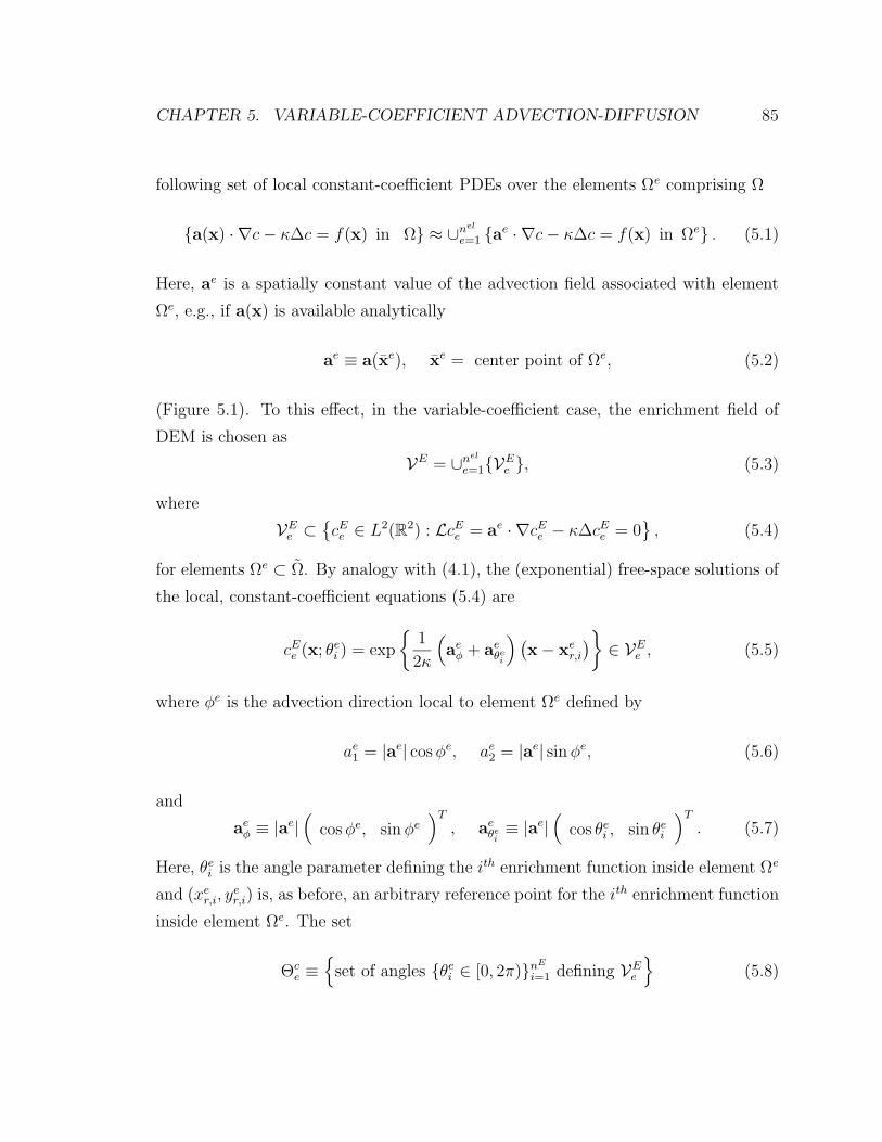
CHAPTER 5. VARIABLE-COEFFICIENT ADVECTION-DIFFUSION 85
following set of local constant-coefficient PDEs over the elements Ωe comprising Ω
a(x) · ∇c− κ∆c = f(x) in Ω ≈ ∪nel
e=1 ae · ∇c− κ∆c = f(x) in Ωe . (5.1)
Here, ae is a spatially constant value of the advection field associated with element
Ωe, e.g., if a(x) is available analytically
ae ≡ a(xe), xe = center point of Ωe, (5.2)
(Figure 5.1). To this effect, in the variable-coefficient case, the enrichment field of
DEM is chosen as
VE = ∪nel
e=1VEe , (5.3)
where
VEe ⊂
cEe ∈ L2(R2) : LcEe = ae · ∇cEe − κ∆cEe = 0
, (5.4)
for elements Ωe ⊂ Ω. By analogy with (4.1), the (exponential) free-space solutions of
the local, constant-coefficient equations (5.4) are
cEe (x; θei ) = exp
1
2κ
(
aeφ + ae
θei
) (x − xe
r,i
)
∈ VEe , (5.5)
where φe is the advection direction local to element Ωe defined by
ae1 = |ae| cosφe, ae
2 = |ae| sinφe, (5.6)
and
aeφ ≡ |ae|
(
cosφe, sinφe)T
, aeθei
≡ |ae|(
cos θei , sin θe
i
)T
. (5.7)
Here, θei is the angle parameter defining the ith enrichment function inside element Ωe
and (xer,i, y
er,i) is, as before, an arbitrary reference point for the ith enrichment function
inside element Ωe. The set
Θce ≡
set of angles θei ∈ [0, 2π)nE
i=1 defining VEe
(5.8)

CHAPTER 5. VARIABLE-COEFFICIENT ADVECTION-DIFFUSION 86
specifying the enrichment space inside element Ωe is defined by analogy with (4.5).
In this case however, the enrichment functions defining VE (4.1) will differ in general
from one element Ωe of the domain to another.
Remark 5.1.1. Although the discussion above has assumed that the diffusivity κ
is spatially constant, so that only a(x), the advection velocity, is allowed to vary,
the approach outlined herein is not limited to the constant diffusivity case. When
κ = κ(x), the enrichment functions for the advection-diffusion equation would be
defined by analogy to (5.5) but with κ(x) frozen locally inside each element.
It is worthwhile to investigate the relation between the local variable-coefficient
enrichment functions comprising (5.4) and the governing variable-coefficient PDE
being solved. Assume that a(x) ∈ C1(Ωe) so that the following Taylor expansion
around the element’s center point xe can be justified:
a(x) = a(xe) + ∇a|x=xe · (x − xe) + O(x − xe)2 in Ωe. (5.9)
The operator governing the PDE (1.2) inside the element Ωe now takes the form
Lc = Lec+ f(c) = 0 in Ωe, (5.10)
where
Lec ≡ a(xe) · ∇c− κ∆c, (5.11)
and
f(c) ≡[∇a|x=xe · (x − xe) + O(x − xe)2
]· ∇c. (5.12)
Equation (5.10) is a perturbed constant-coefficient advection-diffusion equation.
The linearization of a(x) (5.9) is essentially a first order approximation of the ad-
vection field. The free-space solutions to the constant-coefficient problems (5.11) can
therefore be viewed as first order approximations of the free-space solutions of the
variable-coefficient transport equation to be solved. The “residual” advection equa-
tion (5.12) acts as a source-like term. From the discussion of Section 2.3.1, more
specifically, the rule of thumb regarding the inclusion of the polynomial field VP in

CHAPTER 5. VARIABLE-COEFFICIENT ADVECTION-DIFFUSION 87
the approximation space of an enriched element, it follows that the true DEM dis-
cretization is more appropriate for the solution of variable-coefficient problems than
its DGM counterpart, even when such problems are homogeneous. Nevertheless, it
will be shown in Section 5.6 that for some variable-coefficient homogeneous problems,
pure DGM elements with Vh ≡ VE = ∪eVEe defined by (5.4) can perform quite well.
ae ≡(
−yj − h2
xj + h2
)
Ωe
¡¡µ ¢¢
ae′ ≡(
−yj − h2
xj + 3h2
)
Ωe′
xj xj + h xj + 2h
yj
yj + h
¼6a(x) =(−y, x
)T
Figure 5.1: Locally frozen advection fields to enable the construction of enrichmentfunctions as free-space solutions inside the two adjacent elements Ωe = (xj, xj + h)×(yj, yj + h) and Ωe′ = (xj + h, xj + 2h) × (yj, yj + h) for an example advection field
a(x) = (−y, x)T
5.2 The Lagrange multiplier approximation space
Wh
It was shown in Section 2.3.3 that the variational formulation of the problem of
interest implies that the space of approximations of the Lagrange multiplier field
should be related to the normal derivatives of the enrichment functions at the element
edges. The expression for the Lagrange multiplier λ in (2.52) was deduced from
(2.51) for the continuous formulation. A problem arises when one attempts to use
(2.52) to compute appropriate discrete Lagrange multiplier approximations λh in the

CHAPTER 5. VARIABLE-COEFFICIENT ADVECTION-DIFFUSION 88
variable-coefficient context, however. As will be illustrated shortly, this is because
the enrichment field for a generic variable-coefficient problem is element dependent.
5.2.1 Exponential Lagrange multiplier approximations
Suppose that the discrete Lagrange multiplier approximation λh is defined on Γe,e′
analogously to (2.52) — that is, as
λh|Γe,e′ = span
∇cEe (x; θei )|Γe,e′ · ne,e′
, (5.13)
where spancEe (x; θe
i )
is the enrichment field (5.5) inside element Ωe and ne,e′ denotes
the outward unit normal to Γe,e′ . Implicit in the expression (5.13) is the assumption
that ∇cEe ·ne,e′ is defined on Γe,e′ . However, for a non-constant a(x) and the enrichment
space given by (5.3) and (5.4), the normal derivative ∇cEe ·ne,e′ is typically undefined.
For concreteness, consider a discretization of the domain Ω by a (structured or
unstructured) mesh of quadrilateral elements Ωe (Figure 2.1). Let Γe,e′ be a straight
edge separating two adjacent elements Ωe and Ωe′ , but viewed as an edge belonging to
Ωe (Figure 4.4 with h = lij, e = ei and e′ = ej). It is straightforward to parameterize
this edge with respect to an arc-length coordinate 0 ≤ s ≤ h, where h is the length
of this edge (see Section 4.2.1). Denoting by αe,e′ ∈[0, π
2
]the angle Γe,e′ makes with
the x-axis, the normal derivatives of the enrichment functions in elements Ωe and Ωe′
are given by
∇cEe (x; θei )|Γe,e′ · ne,e′ = C1 exp
1
2κ
[(
aeφ + ae
θei
)
· te,e′]
(s− se,e′
r,i )
, (5.14)
and
∇cEe′(x; θe′
i )|Γe′,e · ne′,e = C2 exp
1
2κ
[(
ae′
φ + ae′
θe′i
)
· te,e′]
(s− se,e′
r,i )
, (5.15)
respectively, where C1 ≡ 12κ
(
aeφ + ae
θei
)
· ne,e′ and C2 ≡ 12κ
(
ae′
φ + ae′
θe′i
)
· ne′,e are two
constants, te,e′ is the unit tangent vector to Γe,e′ and 0 ≤ se,e′
r,i ≤ h is an arbitrary
reference point introduced for the stable evaluation of exponentials on Γe,e′ . The

CHAPTER 5. VARIABLE-COEFFICIENT ADVECTION-DIFFUSION 89
argument of the exponential in (5.14) is denoted from this point forward by
Λe(θei ) ≡ Λe
i ≡1
2κ
[(
aeφ + ae
θei
)
· te,e′]
=|ae|2κ
[
cos(φe − αe,e′) + cos(θei − αe,e′)
]
.
(5.16)
From the comparison of (5.14) and (5.15), it follows that if ae 6= ae′ ,
∇cEe (x; θei )|Γe,e′ · ne,e′ 6= −∇cEe′(x; θe′
i )|Γe′,e · ne′,e (5.17)
even for θei = θe′
i . This implies that, in this case, a normal derivative of an enrichment
function along the edge Γe,e′ (5.13) is not well defined.
One approach for remedying the problem exhibited above is to extend the enrich-
ment space V = ∪eVEe (5.3) to the element edges. This extension is denoted here by
VEe,e′ and constructed only for the sake of enabling the approximation of the Lagrange
multiplier field using an approach similar to that of (5.13). For this purpose, let ae,e′
denote a constant advection velocity associated with the edge Γe,e′ , for example,
ae,e′ ≡ a(xe,e′), where xe,e′ = midpoint of Γe,e′ . (5.18)
Then, for a specified angle θe,e′
i ∈ [0, 2π),
cEe,e′(x; θe,e′
i ) ≡ exp
1
2κ
(
ae,e′
φ + ae,e′
θe,e′
i
)(
x − xe,e′
r,i
)∣∣∣∣Γe,e
′
∈ VEe,e′ , (5.19)
is an ith auxiliary enrichment function defined on the edge Γe,e′ . Replacing cEe (x; θi)|Γe,e′by cEe,e′(x; θe,e′
i ) (5.19) in (5.13) leads to the discrete Lagrange multiplier approxima-
tion
λh|Γe,e′ = span
∇cEe,e′(x; θe,e′
i ) · ne,e′
= span
eΛe,e′
i (s−se,e′
r,i ), 0 ≤ s ≤ h
, (5.20)
where
Λe,e′(θe,e′
i ) ≡ Λe,e′
i ≡ 12κ
[(
ae,e′
φ + ae,e′
θe,e′
i
)
· te,e′]
= |ae,e′ |2κ
[
cos(φe,e′ − αe,e′) + cos(θe,e′
i − αe,e′)]
.(5.21)

CHAPTER 5. VARIABLE-COEFFICIENT ADVECTION-DIFFUSION 90
From (5.21) and (5.20), it follows that λh|Γe,e′ = −λh|Γe′,e which implies that λh|Γe,e′is well defined on Γe,e′ .
The approximation (5.20) can be justified by a Taylor analysis. Expanding (5.14)
and the generic function defining the span in (5.20) in a Taylor series leads to
∇cEe (x; θei )|Γe,e′ · ne,e′ = C1
[
1 + Λei (s− se,e′
r,i ) +1
2[Λe
i ]2(s− se,e′
r,i )2 + O(s− se,e′
r,i )3
]
,
(5.22)
so that
λh(s)|Γe,e′ = 1 + Λe,ei (s− se,e′
r,i ) +1
2[Λe,e′ ]2(s− se,e′
r,i )2 + O(s− se,e′
r,i )3, (5.23)
respectively. Since |s− se,e′
r,i | ≤ h, it follows that
∣∣∣∇cE
e (x; θei )|Γe,e′ · ne,e′ − C1λ
h(s)|Γe,e′∣∣∣ = C1
∣∣∣(Λe
i − Λe,e′
i )(s − se,e′
r,i )
+12
(
[Λei ]
2 − [Λe,e′
i ]2)
(s − se,e′
r,i )2 + O(s − se,e′
r,i )3∣∣∣
≤ C1
∣∣∣(Λe
i − Λe,e′
i )h∣∣∣+ O(h2),
(5.24)
which → 0 when h→ 0. A similar result can be established for the difference
∣∣∣∇cEe′(x; θe′
i )|Γe′,e · ne′,e − C2λh(s)|Γe′,e
∣∣∣. (5.25)
The implication of this analysis is that, as the mesh is refined, the normal derivatives
of the enrichment functions cEe and cEe′ inside the adjacent elements Ωe and Ωe′ ap-
proach the normal derivative of the auxiliary enrichment function cEe,e′ (5.19) which is
equally defined on the edges Γe,e′ and Γe′,e. This in turn justifies the choice (5.20) for
approximating the Lagrange multipliers in the case of a variable advection coefficient.
5.2.2 Lagrange multiplier selection
As in the case of the constant-coefficient advection-diffusion equation (Chapter 4),
the set Θce (5.8) typically leads to too many Lagrange multiplier dofs (5.13) in the
sense that condition (2.49) fails. For this reason, the space of Lagrange multiplier

CHAPTER 5. VARIABLE-COEFFICIENT ADVECTION-DIFFUSION 91
approximations is constructed as Wh = ∪e ∪e′<e Whe,e′ where
Whe,e′ ≡ span
∇cEe,e′(x; θλe,e′
i )|Γe,e′ · ne,e′ : θλe,e′
i ∈ Θλe,e′ , n
λ ≡ cardΘλe,e′ =
⌊nE
4
⌋
,
(5.26)
and nλ is the number of Lagrange multiplier dofs per edge.
Recall that, in Section 4.2.2, in the context of a constant-coefficient advection-
diffusion problem, a set of angles, denoted there by Θλ and used for constructing
Lagrange multiplier approximations was chosen independently from the set of angles
Θc used for selecting enrichment functions for the approximation of the primal solu-
tion. In the present chapter, this approach is modified slightly to take into account
an important effect of a varying advection coefficient. Underlying this modification
is the assumption that, to span as well as possible the space of all exponentials of the
form eA : Amin ≤ A ≤ Amax, A should be uniformly distributed between Amin and
Amax. Hence, if
Λe,e′
min ≡ minθλe,e′
i ∈[0,2π)
Λe,e′(θλe,e′
i ) and Λe,e′
max ≡ maxθλe,e′
i ∈[0,2π)
Λe,e′(θλe,e′
i ), (5.27)
where Λe,e′(θλe,e′
i ) is defined as in (5.21), the angles θλe,e′
i are implicitly chosen here
so that the corresponding values of Λe,e′(θλe,e′
i ) are uniformly sampled in the interval
[Λe,e′
min,Λe,e′
max].
The extrema of (5.21) can be computed analytically by taking the derivative of
the function Λe,e′(θ) – which is plotted in Figure 5.2 for straight edges that are aligned
with the x- and y-axes – with respect to θ, setting it to zero, and solving
dΛe,e′
dθ=
|ae,e′ |2κ
sin(αe,e′ − θ∗) = 0
⇒ θ∗ = αe,e′ − nπ, n ∈ Z.(5.28)
Substituting θ∗ = αe,e′ − nπ into (5.21) gives
Λe,e′
min =1
2κ(ae,e′
φ · te,e′ − |ae,e′ |), for θλe,e′
min = αe,e′ + π, (5.29)

CHAPTER 5. VARIABLE-COEFFICIENT ADVECTION-DIFFUSION 92
0 1 2 3 4 5 6 7−0.4
−0.2
0
0.2
0.4
0.6
0.8
1
1.2
1.4
Λe, e′min
Λe, e′max
θλ
Λe,
e′
(a) On edges aligned with the x–axis (α = 0)
0 1 2 3 4 5 6 7−0.4
−0.2
0
0.2
0.4
0.6
0.8
1
1.2
1.4
Λe, e′min
Λe, e′max
θλ
Λe,
e′
(b) On edges aligned with the y–axis(
α =π
2
)
Figure 5.2: Λe,e′(θ) for the case of a quadrilateral element — extrema are marked bycircles (a1 = a2 = κ = 1)
and
Λe,e′
max =1
2κ(ae,e′
φ · te,e′ + |ae,e′ |), for θλe,e′
max = αe,e′ . (5.30)
From (5.29) and (5.30), it follows that the size of the interval [Λe,e′
min,Λe,e′
max] is
∆Λe,e′ ≡ Λe,e′
max − Λe,e′
min =|ae,e′ |κ
. (5.31)
The general procedure for selecting the arguments Λe,e′
i = Λe,e′(θλi ) defining the
approximations of the Lagrange multiplier field is summarized in Algorithm 4 and
illustrated in Figure 5.3. The interval [Λe,e′
min,Λe,e′
max] is partitioned into (nλ − 1) sub-
intervals of equal size, and the union of zero and the (nλ − 1) endpoints of the
subintervals furthest away from zero51 are taken as the set of Λe,e′
i that appears in
the argument of the exponential in (5.20). The approach adopted here is to include
the constant Lagrange multiplier approximation in Whe,e′ , generated by Λe,e′
i = 0.
The constant Lagrange multiplier can be viewed as a coarse scale approximation,
15It is straightforward to show that the function Λe,e′
i (5.16) has necessarily a zero in the interval
(Λe,e′
min,Λe,e′
max), or at one of its endpoints.

CHAPTER 5. VARIABLE-COEFFICIENT ADVECTION-DIFFUSION 93
included in the definition of Whe,e′ in order to balance the fine scales represented by
the remaining (nλ − 1) exponential Lagrange multiplier approximations.
Remark 5.2.1. When ae,e′ ≡ 0 on an edge Γe,e′ — which is the case, for example,
when the advection velocity satisfies a no-slip boundary condition — and nλ > 1, all
of the Lagrange multiplier approximations (5.20) evaluate to constants. To avoid such
a redundancy, polynomial Lagrange multiplier approximations are adopted instead of
exponential ones on edges where |ae,e′ | ≈ 0.
r r r r×Λe,e′
min Λe,e′
maxΛe,e′
i∗0
²¯? r r r r×
Λe,e′
min Λe,e′
max
Λe,e′
1 Λe,e′
4Λe,e′
2 Λe,e′
3
Λe,e′
i∗ ≡ 0
(a) Case 1: |Λe,e′
i∗ | > 12Le,e′ (i∗ = 3)
r r r r×Λe,e′
min Λe,e′
maxΛe,e′
i∗ 0
²? r rr r×
Λe,e′
min Λe,e′
maxΛe,e′
i∗ ≡ 0
Λe,e′
1 Λe,e′
4Λe,e′
2 Λe,e′
3
(b) Case 2: |Λe,e′
i∗ | < 12Le,e′ (i∗ = 2)
r r r r×Λe,e′
min Λe,e′
maxΛe,e′
i∗ 0
²? r rr r×
Λe,e′
min Λe,e′
maxΛe,e′
i∗ ≡ 0
Λe,e′
1 Λe,e′
4Λe,e′
2 Λe,e′
3
(c) Case 3: |Λe,e′
i∗ | = 12Le,e′ (i∗ = 2)
Figure 5.3: Illustration of the Lagrange multiplier selection procedure (Algorithm 4)for nλ = 4

CHAPTER 5. VARIABLE-COEFFICIENT ADVECTION-DIFFUSION 94
Algorithm 4 Construction of the Lagrange multiplier approximation field
Given nE exponential enrichment functions (5.5), set nλ =⌊
nE
4
⌋
per (2.50).
Select a tolerance δ > 0, δ << 1.for all edges Γe,e′ in the mesh do
if |ae,e′ | < δ thenEmploy polynomial Lagrange multipliers on Γe,e′ .
elseCompute Λe,e′
min and Λe,e′
max using (5.29) and (5.30) respectively.Set
Le,e′ ≡ ∆Λe,e′
(nλ − 1)=
|ae,e′ |κ(nλ − 1)
. (5.32)
for i = 1 to nλ doSet
Λe,e′
i = Λe,e′
min + (i− 1)Le,e′ . (5.33)
end forFind the index
i∗ = min
argmin1≤i≤nλ |Λe,e′
i |
. (5.34)
Set Λe,e′
i∗ = 0.
Return the set Λe,e′
i nλ
i=1 and define the Lagrange multipliers as in (5.20).end if
end for
5.3 Augmentation of VE
Numerical tests (Section 5.6) suggest that the performance of DEM when applied to
some variable-coefficient transport problems can be improved by adding to the space
of exponential enrichment functions (5.5) some of the other free-space solutions to
(1.2) derived in Chapter 3.
5.3.1 Augmentation of VE by polynomial free-space solutions
to the 2D advection-diffusion equation
In Chapter 3, a family of polynomial free-space solutions to the advection-diffusion
equation with constant coefficients (1.2) was derived (Section 3.1.2). Up to this

CHAPTER 5. VARIABLE-COEFFICIENT ADVECTION-DIFFUSION 95
point, these polynomial free-space solutions were not included in the design of the
enrichment space VE. It was found numerically (Section 4.5) that DEM performed
quite well without these polynomial enrichment functions, and indeed our objective
was to capture exponential boundary layers.
In an attempt to make VEe as rich as possible given the information available, the
following definition of VEe (5.4) is proposed
VEe ≡ Vexp
e ⊕ Vpole , (5.35)
where
Vexpe ≡
cEe ∈ L2(Ω) : c|EΩe(x, y) =nexp∑
i=1
cicexpe,i (x; θe
i ), ci ∈ R
, (5.36)
cexpe,i (x; θe
i ) = e
„
ae1+|ae| cos θei2κ
«
(x−xer,i)e
„
ae2+|ae| sin θei2κ
«
(y−yer,i), 0 ≤ θe
i < 2π, (5.37)
and
Vpole ≡
cE ∈ L2(Ω) : c|EΩe(x, y) =
npol−1∑
i=0
cicpole,i (x), ci ∈ R
. (5.38)
From Section 3.1.2,
cpole,0 (x) = 1, (5.39)
cpole,1 (x) = |ae
2x− ae1y|, (5.40)
cpole,2 (x) = (ae
2x− ae1y)
2 + 2(ae · x), (5.41)
cpole,3 (x) = (ae
2x− ae1y)
3 + 6(ae2x− ae
1y)(ae · x), (5.42)
in (5.38), and so on, where it is recalled that ae ≡ ae/κ. Note that Vexp (5.36) is
exactly the exponential enrichment space spanned by the functions (5.5).
Remark 5.3.1. For constant-coefficient problems (Chapter 4), the enrichment space
VE can be defined by the direct sum (5.35) as well, if desired.
Remark 5.3.2. To avoid possible linear dependence of the functions cpole,n(x) (5.38)
with the standard Galerkin polynomial shape functions comprising VP , the rule of

CHAPTER 5. VARIABLE-COEFFICIENT ADVECTION-DIFFUSION 96
thumb of excluding VP from Vh when designing elements for which VEe is given by
(5.35) will be adopted. That is, elements for which VEe is given by (5.35) will be, by
construction, pure DGM elements (second line of (2.38)) – Section 5.4.
5.3.2 Augmentation of VE by a “higher order” enrichment
function
The enrichment functions comprising the space (5.35) can be viewed as first order
enrichment functions for a variable-coefficient advection-diffusion BVP, in the sense
that these functions solve (1.2) with a(x) linearized to first order:
a(x) ≈ a(xe) in Ωe. (5.43)
Defining the enrichment spaces in this way may limit the performance of DEM when
the method is used to solve variable-coefficient problems. To address this possible
limitation, suppose a(x) is linearized to second order instead of to first order (5.43),
that is:
a(x) ≈ a(xe) + ∇a|x=xe · (x − xe) in Ωe, (5.44)
where ∇a|x=xe denotes the advection gradient tensor evaluated at the element mid-
point xe:
∇a|x=xe =
(∂a1
∂x(xe) ∂a1
∂y(xe)
∂a2
∂x(xe) ∂a2
∂y(xe)
)
. (5.45)
With the approximation (5.44), (1.2) is of the form
[Aex + be] · ∇c− ∆c = 0, (5.46)
where
Ae ≡ ∇a|x=xe
κ, be ≡
(ae
κ− ∇a|x=xe
κxe
)
. (5.47)
The free-space solutions to the variable-coefficient advection-diffusion equation
(5.46) were derived in Section 3.2. Hence, the approximation space VEe described

CHAPTER 5. VARIABLE-COEFFICIENT ADVECTION-DIFFUSION 97
earlier can be augmented as follows:
VEe ≡ Vexp
e ⊕ Vpole ⊕ Verf
e , (5.48)
where
Verfe ≡ span
erf
(√−2σe
−2
(
ve− · x +
ve− · be
σe−
))
, (5.49)
with
(σe−,v
e−) ≡ (σ,v) : Aev = σv, σ ∈ R, σ < 0 . (5.50)
That is, σe− in (5.49) is the negative real eigenvalue, if there is such an eigenvalue, of
Ae (5.47) and ve− is its corresponding eigenvector2. The enrichment comprising Verf
e
(5.49) can be viewed as a “higher order” enrichment. It is “higher order” in the sense
that a linear combination of this function and a constant, namely
cE(x) =∫ vi·x0
exp
σi2w2 + [vi · b]w
dw
=√
2π2√−σi
exp
−(vi·b)2
2σi
[
erf(√
−2σi2
[
(vi · x) + vi·bσi
])
+ erf(√
2(vi·b)
2√−σi
)]
,
(5.51)
as shown in Section 3.2, solves
[ae + ∇a|x=xe(x − xe)] · ∇c− κ∆c = 0. (5.52)
Remark 5.3.1. The following are some connections between the character of the
functions (5.49) and the physics of the flow field a(x):
• In the case when a(x) represents the velocity field, ∇a is the velocity gradient
tensor.
• In the case of an incompressible flow (∇ · a = 0), tr(A) = 0, so that the
eigenvalues (5.50) simplify to:
σ± = ±√
∆, (5.53)
2It can be shown that if a(x) is incompressible and has real eigenvalues, one of these eigenvaluesis necessarily negative; Remark 5.3.1.

CHAPTER 5. VARIABLE-COEFFICIENT ADVECTION-DIFFUSION 98
which are either purely real or purely imaginary, where ∆ was defined earlier in
(3.52).
• In an irrotational (2D) flow, ∇a is symmetric. A consequence of this fact is
that all its eigenvalues are real.
• In a fluid mechanics context, when I(∇a) 6= 0, we are in a region known as the
vortex core of the flow [64].
Remark 5.3.2. The higher order function (5.49) is employed only inside elements
for which ∇a|x=xe has a negative, real eigenvalue. When σ > 0 or I(σ) 6= 0 (where
I(z) denotes the imaginary part of a complex number z ∈ C), the functions specified
by (5.49) are not good representations of the solutions to the sorts of boundary value
problems considered here, as suggested by the LLS qualifying test described in Section
2.5.
5.4 DGM and DEM element design
5.4.1 Nomenclature and computational complexity
In this section, several low and higher-order quadrilateral DGM and DEM elements
are proposed for the solution to variable-coefficient transport problems. The nota-
tion used for describing these elements is summarized in Table 5.1. As before, ‘Q’
Table 5.1: DGM and DEM Element Nomenclature
Element Type VE Notation
DGM(Vh = VE)
Vexp Q-nexp-nλ
Vpol ⊕ Vexp Q-(npol, nexp)-nλ
Vpol ⊕ Vexp ⊕ Verf Q-(npol, nexp)∗-nλ
DEM(Vh = VP ⊕ VE)
Vexp Q-nexp-nλ+
Vexp ⊕ Verf Q-nexp∗-nλ+

CHAPTER 5. VARIABLE-COEFFICIENT ADVECTION-DIFFUSION 99
stands for quadrilateral. The integers nexp and npol denote the number of exponen-
tial enrichment functions (cardinality of the set Θce) and the number of polynomial
enrichment functions (deg(Vpol) + 1), respectively. The integer nλ is the number of
Lagrange multiplier dofs per edge (cardinality of the set Λe,e′
i ). The + superscript
designates a true DEM element (Vh = VP ⊕ VE) and distinguishes it from a pure
DGM element (Vh = VE). The polynomial approximation VP of all four considered
DEM elements is chosen to be that of the standard bilinear element Q1. The ∗ super-
script indicates that the enrichment space of the element has been augmented by the
“higher order” error function enrichment (5.49). For the Q-(npol, nexp)∗-nλ elements,
nE = nexp + npol + 1. Otherwise, for the Q-(npol, nexp)-nλ and Q-(npol, nexp)-nλ+
elements, nE = nexp + npol; for the Q-nexp-nλ and Q-nexp-nλ+ elements, nE = nexp.
In this section, proposed first are four DGM elements Q-4-1, Q-8-2, Q-12-3 and
Q-16-4 and four DEM elements Q-5-1+, Q-9-2+, Q-13-3+ and Q-17-4+ for which
VE = Vexp. For all of these elements, Θce is chosen as
Θce = θe
mnE
m=1 ≡ φe + βmnE
m=1 with βm =2(m− 1)π
nE∈ [0, 2π), (5.54)
where nE = nexp. (5.54) leads to the specifications of Table 5.2.
Proposed also are four additional DGM elements Q-(4, 0)-1, Q-(4, 5)-2, Q-(4, 9)-3
and Q-(4, 13)-4 for which VE = Vpol ⊕ Vexp. The specifications of these elements
are summarized in Table 5.2 as well. For each of these elements npol = 4, so that
Vpol consists of polynomial free-space solutions to the constant-coefficient advection-
diffusion equation up to degree three (5.39)–(5.42). For the first element, denoted by
Q-(4, 0)-1, nexp = 0, so that VE = Vpol.
The computational complexities and stencil widths of the DGM and DEM ele-
ments just described can be inferred from Table 2.2 for the case of a uniform mesh
with nel = n × n quadrilateral elements, assuming that static condensation of the
enrichment dofs is implemented at the element-level (see Section 2.4.2). Some of the
elements’ key computational properties are summarized below.
• The stencil of a DGM discretization is in general smaller than that of its
Galerkin comparable.

CHAPTER 5. VARIABLE-COEFFICIENT ADVECTION-DIFFUSION 100
Table 5.2: Enrichment spaces of the proposed DGM and DEM elements for variable-coefficient transport problems
Element nE Θce degVpol
DGM element
Q-4-1 4 φe +π
2(m− 1) : m = 1, ..., 4
−Q-(4, 0)-1 4 − 3Q-(4, 0)∗-1 5 − 3
Q-8-2 8 φe +π
4(m− 1) : m = 1, ..., 8
−
Q-(4, 5)-2 9 φe +
2π
5(m− 1) : m = 1, ..., 5
3
Q-(4, 5)∗-2 10 φe +
2π
5(m− 1) : m = 1, ..., 5
3
Q-12-3 12 φe +π
6(m− 1) : m = 1, ..., 12
−
Q-(4, 9)-3 13 φe +
2π
9(m− 1) : m = 1, ..., 9
3
Q-(4, 9)∗-3 14 φe +
2π
9(m− 1) : m = 1, ..., 9
3
Q-16-4 16 φe +π
8(m− 1) : m = 1, ..., 16
−
Q-(4, 13)-4 17 φe +
2π
13(m− 1) : m = 1, ..., 13
3
Q-(4, 13)∗-4 18 φe +
2π
13(m− 1) : m = 1, ..., 13
3
DEM element
Q-5-1+ 5 φe +
2π
5(m− 1) : m = 1, ..., 5
−
Q-9-2+ 9 φe +
2π
9(m− 1) : m = 1, ..., 9
−
Q-13-3+ 13 φe +
2π
13(m− 1) : m = 1, ..., 13
−
Q-17-4+ 17 φe +
2π
17(m− 1) : m = 1, ..., 17
−
• Any two elements of the following quadruples of DGM and Galerkin elements
have comparable computational complexity: (Q-4-1,Q-(4, 0)-1, Q-(4, 0)∗-1, Q1),
(Q-8-2, Q-(4, 5)-2, Q-(4, 5)∗-2, Q2), (Q-12-3, Q-(4, 9)-3, Q-(4, 9)∗-3, Q3) and (Q-
16-4, Q-(4, 13)-4, Q-(4, 13)∗-4, Q4).

CHAPTER 5. VARIABLE-COEFFICIENT ADVECTION-DIFFUSION 101
• Each constructed DEM element Q-nE-nλ+ and Q-nE∗-nλ+ has the same com-
putational complexity as the standard Galerkin element Qnλ+1.
5.4.2 Lagrange multiplier selection
For all DGM and DEM elements summarized in Table 5.2, the Lagrange multiplier
approximations are constructed via the Lagrange multiplier approximation procedure
developed in Section 5.2. The sets of exponential arguments Λe,e′
i associated with these
elements are specified in Table 5.3.
Table 5.3: Lagrange multiplier approximation spaces of the DGM and DEM elementsin Table 5.2 (identified here by the number of Lagrange multiplier dofs per edge, nλ)
nλ Λe,e′
i ⊆ Θλe,e′ ⊆ λe,e′
h ⊆1 0 φe,e′ + π 12 0,Λe,e′
min,Λe,e′
max φe,e′ + π, αe,e′ + π, αe,e′
1, exp(
12κ
ae,e′
φ · te,e′ ∓ 12κ|ae,e′ |
)
3
0,Λe,e′
mp ,φe,e′ + π, αe,e′ + π
2,
1, exp(
12κ
ae,e′
φ · te,e′)
,
Λe,e′
min,Λe,e′
max
αe,e′ + π, αe,e′
exp(
12κ
ae,e′
φ · te,e′ ∓ 12κ|ae,e′ |
)
4
0,Λe,e′
min,Λe,e′
max ,φe,e′ + π, αe,e′ + π, αe,e′
1, exp(
12κ
ae,e′
φ · te,e′ ∓ 12κ|ae,e′ |
)
,
Λe,e′
mp ± 16∆Λe,e′
αe,e′ + cos−1
(∓1
3
)exp
(12κ
ae,e′
φ · te,e′ ∓ 16κ|ae,e′ |
)
The following analysis suggests that the Lagrange multiplier selection procedure
detailed in Section 5.2.2 is appropriate for the Q-(npol, nexp)-nλ elements in Table 5.2.
From Section 3.1.2, an nth degree polynomial free-space solution cpoln (x) to (1.2)
has the form
cpoln (x) = |a × x|n + fn(x, y), (5.55)
where fn(x, y) is an n− 1 degree polynomial. Now, on an edge Γij (4.13),
|a × x|n|Γij = |(a × xij0 ) + (a × tij)s|n. (5.56)

CHAPTER 5. VARIABLE-COEFFICIENT ADVECTION-DIFFUSION 102
Taking the normal derivative of the expression in (5.56) along an edge Γij, it fol-
lows that the polynomial enrichment functions (5.55) give rise to Lagrange multiplier
approximations of the form
λh(s)|Γij =npol−2∑
k=0
λksk, 0 ≤ s ≤ lij. (5.57)
That is, if Vpol consists of polynomials up to degree npol − 1, then the Lagrange
multiplier approximations should be polynomials up to degree npol−2. By the rule of
thumb (2.50) (Remark 2.3.2), only bnpol/4c Lagrange multiplier approximations per
edge are to be retained. Now, observe that, for k >> 1 and h → 0, sk → 0. Hence,
it is reasonable to approximate the Lagrange multiplier approximations (5.57) by
λh(s)|Γij =
nλpol∑
k=0
λksk, 0 ≤ s ≤ lij, (5.58)
where
nλpol =
⌊npol
4
⌋
. (5.59)
For the elements in Table 5.2, npol = 4 so that (5.59) evaluates to nλpol = 1. For
nλpol = 1, (5.58) is simply the constant approximation. But the constant λh = 1
approximation is, by construction, already contained in the space Whij (Section 5.2).
This suggests that the Lagrange multiplier selection algorithm developed in Section
5.2 need not be modified for the elements Q-(4, 0)-1, Q-(4, 5)-2, Q-(4, 9)-3 and Q-
(4, 13)-4.
5.5 Implementation and computational properties
5.5.1 Analytical evaluation of element-level arrays
As in the constant-coefficient DEM, when κ→ 0 (Pe→ ∞), the numerical integration
by a Gaussian quadrature of the integrals (2.22)–(2.25) becomes highly inaccurate
because of the large magnitudes of the arguments of the exponential enrichment

CHAPTER 5. VARIABLE-COEFFICIENT ADVECTION-DIFFUSION 103
functions (5.36). It was shown in Section 4.4.2 that these integrals can be computed
analytically on a mesh with straight-edged elements whose edges are aligned with
the coordinate axes if a is spatially constant. In general, these integrals can still
be evaluated analytically on any mesh with straight-edged elements aligned with the
coordinate axes, provided that the advection field a(x) is a sufficiently simple function.
For example, on a uniform mesh of square elements Ωe ≡ (xj, xj+1) × (yj, yj+1), the
entries of the kEE matrices (2.56), for 1 ≤ l,m ≤ nE, take the form
kEElm ≡
∫
Ωe[(a(x) · ∇cl)cm + κ∇cl · ∇cm]dΩe
=|ae|2κ
(cosφe + cos θel )I
a1(x)lm +
|ae|2κ
(sinφe + sin θel )I
a2(x)lm
+1
4κ[(aφ + aθl) · (aφ + aθm)] Idiff
lm ,
(5.60)
where
Iai(x)lm ≡
∫ xj+1
xj
∫ yj+1
yjai(x)e
|ae|2κ
(2 cos φe+cos θel+cos θem)(x−xer,l−xer,m)×e
|ae|2κ
(2 sin φe+sin θel+sin θem)(y−yer,l−yer,m)dydx,(5.61)
for i = 1, 2, and
Idifflm ≡
[∫ xj+1
xje
|ae|2κ
(2 cos φe+cos θel+cos θem)(x−xer,l−xer,m)dx]
×[∫ yj+1
yje
|ae|2κ
(2 sin φe+sin θel+sin θem)(y−yer,l−yer,m)dy]
.(5.62)
The diffusion integral Idifflm (5.62) can be evaluated analytically as it is simply the prod-
uct of two one-dimensional integrals of exponential functions. Analytic computation
of the advection integrals Iai(x) (5.61) depends on the form of a(x). For a polynomial
ai(x), e.g., ai(x) = xmiyni for some integers mi and ni, a recursive relation can be
derived to compute (5.61) exactly with ease.
In practice, a(x) is likely to be available numerically — that is, at a discrete set of
N points xe1, ...,x
eN ∈ Ωe. In this case, a(x) can be reconstructed by interpolating
its discrete values at these points using standard Lagrange polynomial interpolation
within each element (Section 5.5.3), making possible the analytic computation of

CHAPTER 5. VARIABLE-COEFFICIENT ADVECTION-DIFFUSION 104
(5.61).
5.5.2 Scaling of enrichment functions
To avoid evaluating a very large floating point number on a finite precision arithmetic
machine, the exponential enrichment functions (5.36) are scaled by the effect of an
arbitrary reference point xer,i within each element Ωe per the procedure outlined in
Section 4.4.3 (Algorithm 3). The polynomial enrichment functions (5.38) are scaled
as well to prevent numerical overflow and improve matrix conditioning. They are
normalized as follows:
cpole,n(x) =
cpole,n(x)
maxx∈Ωe |cpole,n(x)|
, (5.63)
within each element Ωe.
5.5.3 Interpolation of advection field
In practical applications, the advection field a(x) may not be available in closed
analytic form. Suppose the advection field a(x) is available at a discrete set of N
points, x1, ...,xN : ai : i = 1, ..., N, where ai ≡ a(xi). In this case (Sections 5.6.3–
5.6.4), the a(x) that appears in the bilinear form (2.22) will be interpolated from these
discrete values using some appropriate set of interpolation functions. For example,
if the interpolation functions are isoparametric shape functions based on Lagrange
polynomials, a(x) is interpolated inside element Ωe as
ae(ξ) =
# nodes of Ωe∑
i=1
aeiφ
ei (ξ), (5.64)
where ξ ∈ [−1, 1]2 is the usual parent coordinate system (Section 7.1.1), φei (ξ) are
the interpolation functions and aei are the values of the advection field at the nodes
of an element Ωe.

CHAPTER 5. VARIABLE-COEFFICIENT ADVECTION-DIFFUSION 105
5.6 Numerical results
The performances of the DGM and DEM elements described in the previous section
are assessed on four different two-dimensional linear variable-coefficient transport
problems. In each of these problems, the boundary conditions for (1.2) are prescribed
so that boundary layers form as κ → 0 (Pe → ∞), making the solution of these
problems by a standard FEM inefficient. The first two problems are:
• An inhomogeneous BVP with a rotating advection field posed on an L–shaped
domain [Section 5.6.1].
• A homogeneous BVP with a linear advection field, referred to as the “thermal
boundary value problem” [Section 5.6.2].
In these problems, a(x) is given in closed analytical form. It is shown that DEM
can outperform the standard and stabilized Galerkin FEM by a large margin with-
out augmenting the exponential enrichment space (5.36) with additional enrichment
functions, as proposed in Section 5.3.
The last two problems considered in this section are:
• A homogeneous BVP modeling a lid-driven cavity flow [Section 5.6.3].
• A homogeneous BVP posed inside a differentially-heated square cavity [Section
5.6.4].
The advection field a(x) for these problems is obtained by solving an initial boundary
value problem (IBVP) for the time-dependent, incompressible (or near-incompressible)
2D Navier-Stokes equations, and converging this solution to a steady state. Since a(x)
is computed numerically, it is available at a discrete set of points in the domain, rather
than in closed analytical form as in the case of the former two problems. The a(x)
that appears in the bilinear form defining the stiffness matrices is interpolated in-
side each element from these discrete points using Lagrange polynomial interpolation
functions, following the procedure outlined in Section 5.5.3. For the latter two test

CHAPTER 5. VARIABLE-COEFFICIENT ADVECTION-DIFFUSION 106
cases, it is shown that the accuracy of the DEM solution can be improved by aug-
menting the exponential enrichment space V expe by additional free-space solutions to
variants of the governing equation, as described in Section 5.3.
In all problems, the given domain Ω is discretized by uniform meshes of square
elements. For the problems of Sections 5.6.1 and 5.6.2, the performances of the
considered DGM and DEM elements are contrasted with those of their standard
Galerkin comparables. The performances of the DGM elements Q-4-1 and Q-(4, 0)-
1 and DEM elements Q-5-1+ are also compared to that of the streamline upwind
stabilized bilinear finite element proposed in [16]. All reported solution errors are
relative solution errors measured in the L2(Ω) broken norm (4.34), where cref(x) is
a converged “reference” solution computed using a sufficiently refined mesh. The
adoption here of a reference solution in lieu of an exact one is due to the fact that the
exact solutions of the BVPs considered in the subsequent subsections are unavailable.
It is verified that the reference solutions employed in the error analysis are free from
any spurious oscillations.
5.6.1 Inhomogeneous problem with a rotating advection field
and an L–shaped domain
Here, the following inhomogeneous BVP defined on an L-shaped domain Ω = [(0, 1)×(0, 1)]\[(0, 0.5) × (0.5, 1)] (Figure 5.4) is considered
(
1 − y, x)T
· ∇c(x) − κ∆c(x) = 1, in Ω = [(0, 1) × (0, 1)]\[(0, 0.5) × (0.5, 1)],
c = 0, on ∂Ω.
(5.65)
The diffusivity constant is set to κ = 10−3, so that the Peclet number for this problem
is Pe = 103. This problem is a variable-coefficient variant of an advection-diffusion
problem that was studied in [63] and Section 4.5.4. It is also similar to a benchmark
problem that was used to evaluate the performances of the residual-free bubbles and
Petrov-Galerkin stabilized methods in [14] and [23], respectively. The advection field
represents a rigid body rotation about the point (x, y) = (0, 1).

CHAPTER 5. VARIABLE-COEFFICIENT ADVECTION-DIFFUSION 107
-
6
Ω
c = 0
c = 0
c = 0
c = 0
c = 0
c = 0c = 0
aT =(
1 − y, x)
1 x
1
y
0.5
0
Figure 5.4: L-shaped domain and rotating velocity field, with curved lines indicatingstreamlines (Section 5.6.1)
The above problem is a stringent test for the advection-diffusion equation because
its solution presents an outflow boundary layer as well as a second boundary layer
which terminates in the vicinity of the reentrant corner(the point (x, y) = (0.5, 0.5)
in Figure 5.4). Because it is an inhomogeneous problem, the DEM elements Q-5-
1+, Q-9-2+, Q-13-3+ and Q-17-4+ are more suitable for its discretization than their
DGM counterparts. The performances of these elements obtained for this problem
are reported in Table 5.4 for four different mesh resolutions. In each case, these
performances are contrasted with those of the standard Galerkin elements Q1, Q2,
Q3 and Q4, and that of the stabilized version of the finite element Q1. The results
are tabulated by groups of elements of comparable convergence rates. The reference
solution employed in the error analysis is computed using the higher-order Galerkin
element Q6 and a uniform mesh with an element size h = 1/120.
The reader can observe that in general, each considered DEM element delivers
for a given mesh an accuracy that is an order of magnitude better than that of its
standard Galerkin comparable. The DEM element Q-5-1+ is also found to outperform
the stabilized finite element Q1 [16] by a large margin.
Table 5.5 reports the convergence rates numerically deduced from the performance
results reported in Table 5.4. Each pair of elements (Q1, Q-5-1+), (Q2, Q-9-2+),

CHAPTER 5. VARIABLE-COEFFICIENT ADVECTION-DIFFUSION 108
Table 5.4: Inhomogeneous problem of Section 5.6.1 defined on an L-shaped domain(Pe = 103): relative solution errors
Element 300 elements 1, 200 elements 2, 700 elements 10, 800 elements
Q1 4.91 × 101 2.28 × 10⁻¹ 1.46 × 10⁻¹ 6.33 × 10⁻²
Stabilized Q1 2.26 × 10⁻¹ 1.39 × 10⁻¹ 1.02 × 10⁻¹ 5.54 × 10⁻²
Q-5-1+ 1.29 × 10⁻¹ 3.87 × 10⁻² 2.16 × 10⁻² 7.36 × 10⁻³
Q2 2.02 × 10⁻¹ 9.13 × 10⁻² 5.44 × 10⁻² 1.90 × 10⁻²
Q-9-2+ 4.40 × 10⁻² 1.24 × 10⁻² 5.85 × 10⁻³ 1.13 × 10⁻³
Q3 1.12 × 10⁻¹ 4.58 × 10⁻² 2.46 × 10⁻² 6.29 × 10⁻³
Q-13-3+ 3.10 × 10⁻² 6.85 × 10⁻³ 2.10 × 10⁻³ 2.24 × 10⁻⁴
Q4 6.89 × 10⁻² 2.45 × 10⁻² 1.13 × 10⁻² 1.92 × 10⁻³
Q-17-4+ 2.74 × 10⁻² 2.42 × 10⁻³ 4.92 × 10⁻⁴ 1.24 × 10⁻⁴
(Q3, Q-13-3+) and (Q4, Q-17-4+) is found to have a comparable convergence rate.
However, Figure 5.5 shows that in each case, the DEM element has the smallest
constant: for a given mesh size, it delivers a numerical solution that is typically one
order of magnitude more accurate than those produced by its standard and stabilized
Galerkin comparables. More specifically, the reader can observe that to achieve for
this problem the relative error of 0.1%:
• The DEM element Q-5-1+ requires 6.4 times fewer dofs than the Galerkin ele-
ment Q1.
• The DEM element Q-9-2+ requires 8.3 times fewer dofs than the Galerkin ele-
ment Q2.
• The DEM element Q-13-3+ requires 5.7 times fewer dofs than the Galerkin
element Q3.
• The DEM element Q-17-4+ requires 4.3 times fewer dofs than the Galerkin
element Q4.
These results demonstrate the computational superiority of the DEM methodology.

CHAPTER 5. VARIABLE-COEFFICIENT ADVECTION-DIFFUSION 109
The performance results reported in Table 5.5 also reveal that increasing the
number of enrichment functions of a DEM element reduces the number of dofs needed
for achieving a specified accuracy, thereby illustrating the higher-order behavior of a
DEM element with an increasing value of nE.
Table 5.5: Inhomogeneous problem of Section 5.6.1 defined on an L-shaped domain(Pe = 103): convergence rates
Element Convergence rate∗Required # dofs to achievethe relative error of 10−2
Q1 1.44 139, 649Stabilized Q1 1.16 198, 020
Q-5-1+ 1.55 21, 834Q2 1.94 62, 721
Q-9-2+ 2.37 7, 568Q3 2.67 33, 707
Q-13-3+ 3.23 5, 935Q4 3.50 20, 796
Q-17-4+ 3.26 4, 802
* The convergence rates reported in Table 5.5 for the standard Galerkin elements are slightly below the the-oretical rates associated with the L2 norm, because they are derived from numerical experiments and meshresolutions for which these elements have not reached asymptotic convergence.

CHAPTER 5. VARIABLE-COEFFICIENT ADVECTION-DIFFUSION 110
10−2
10−1
10−4
10−3
10−2
10−1
100
Mesh size h
rela
tive
erro
r
L−shaped rotating field, inhomogeneous problem, Pe = 1000
Q
1
Stabilized Q1
Q−5−1+
Q2
Q−9−2+
Q3
Q−13−3+
Q4
Q−17−4+
Figure 5.5: Inhomogeneous problem of Section 5.6.1 defined on an L-shaped domain(Pe = 103): decrease of the relative solution error with the mesh size
5.6.2 Thermal boundary layer problem
Next, the following variable-coefficient BVP, whose boundary conditions are illus-
trated in Figure 5.6, is considered
(
y, 0)T
· ∇c(x) − κ∆c(x) = 0, in Ω = (0, 1)2,
c(0, y) = 1, 0 ≤ y ≤ 1,
c(1, y) = y, 0 ≤ y ≤ 1,
c(x, 0) = 1 − x
ε, 0 ≤ x ≤ ε,
c(x, 0) = 0, ε ≤ x ≤ 1,
c(x, 1) = 1, 0 ≤ x ≤ 1.
(5.66)
The parameter 0 < ε << 1 ensures that the above BVP is well-posed. It is set here
to ε = 1/10. The diffusivity constant is set to κ = 10−3, which sets the Peclet number

CHAPTER 5. VARIABLE-COEFFICIENT ADVECTION-DIFFUSION 111
to Pe = 103. Variants of this problem have been used to assess the performance of
stabilized finite elements [20, 22, 23] and other finite elements with enriched approx-
imation spaces [53, 65]. This problem is referred to here as a thermal boundary layer
problem as it may be viewed as a model problem for the formation of a pair of thermal
boundary layers along the lower and outflow boundaries of a fully developed shear
flow between two parallel plates with the lower one fixed, and the upper one moving
to the right. In this context, c(x) represents the temperature at a point x ∈ Ω ⊂ R2.
This BVP involves a relatively simple variable advection field. However, its solution
features both an outflow boundary layer at x = 1, and a parabolic layer along y = 0.
As such, it is a challenging problem for standard Galerkin elements(see Figures 5.7
and 5.8 (a),(c), (e)).
-
6
¡¡¡¡¡¡¡¡¡¡¡¡
-
-
-
aT =(y, 0
)
-c = 1
1
c = y
c = 1
10
y
xε︸︷︷︸
c = 1 − xε
︸ ︷︷ ︸
c = 0
Figure 5.6: Thermal boundary layer problem of Section 5.6.2: domain and boundaryconditions
Table 5.6 reports the relative solution errors associated with the discretization of
the above problem by the variable-coefficient variants of the DGM and DEM elements
introduced Section 4.3, and standard and stabilized Galerkin using four different
uniform meshes. As for the problem of Section 5.6.1, the error analysis is performed
with respect to a reference solution computed using the higher-order Galerkin element
Q6 and a uniform mesh with an element size h = 1/120. In the first column of this

CHAPTER 5. VARIABLE-COEFFICIENT ADVECTION-DIFFUSION 112
table, n denotes the number of elements in one direction. Therefore, the total number
of elements is nel = n2 and the size of an element is h =1
n. Figure 5.7 and Figure
5.8 display the front and rear views of the standard Galerkin and DGM solutions,
respectively. The following observations are noteworthy:
• Although the first-order DGM element Q-4-1 is outperformed by the DEM
element Q-5-1+ which has a slightly higher computational complexity, the Q-4-
1 element outperforms both the standard and stabilized Galerkin elements Q1
which have a comparable computational complexity.
• Despite the fact that the homogeneous problem considered here is a variable-
coefficient BVP and therefore locally equivalent to an inhomogeneous constant-
coefficient problem(see (5.10)–(5.12)
), the DGM elements are found to become
as effective as the DEM elements at solving it when more enrichment functions
are added to VEe .
• In general, the DGM and DEM elements are found to deliver for a given mesh a
significantly better accuracy than their standard Galerkin comparables. When
the number of enrichment functions is increased, the higher-order DGM and
DEM elements are shown to produce numerical solutions that are an order of
magnitude more accurate than those computed by their standard higher-order
Galerkin comparables.
• Whereas the solutions computed using the DGM and DEM discretizations are
continuous and smooth, those computed using the Galerkin discretizations —
including the higher-order ones — are contaminated by spurious, non-physical
oscillations near the outflow boundary (x = 1).
5.6.3 Lid-driven cavity flow problem
The lid-driven cavity flow problem is a well known validation problem for codes
and numerical methods in the field of computational fluid mechanics. The problem is
posed on a simple two-dimensional (2D) square domain Ω ≡ (0, 1)2 ∈ R2, representing

CHAPTER 5. VARIABLE-COEFFICIENT ADVECTION-DIFFUSION 113
Table 5.6: Thermal boundary layer problem of Section 5.6.2 (Pe = 103): relativesolution errors
Element n = 10 n = 15 n = 20 n = 30
Q1 4.00e × 10−1 1.16 × 10⁻¹ 9.47 × 10⁻² 5.74 × 10⁻²
Stabilized Q1 8.42 × 10⁻² 6.55 × 10⁻² 5.49 × 10⁻² 4.20 × 10⁻²
Q-4-1 6.48 × 10⁻² 4.97 × 10⁻² 3.79 × 10⁻² 2.25 × 10⁻²
Q-5-1+ 1.22 × 10⁻² 7.07 × 10⁻³ 4.25 × 10⁻³ 2.12 × 10⁻³
Q2 9.54 × 10⁻² 5.10 × 10⁻² 3.62 × 10⁻² 2.20 × 10⁻²
Q-8-2 2.10 × 10⁻² 9.37 × 10⁻³ 4.43 × 10⁻³ 1.50 × 10⁻³
Q-9-2+ 4.62 × 10⁻³ 4.56 × 10⁻³ 9.71 × 10⁻⁴ 5.56 × 10⁻⁴
Q3 4.52 × 10⁻² 2.72 × 10⁻² 1.87 × 10⁻² 1.04 × 10⁻²
Q-12-3 5.55 × 10⁻³ 3.98 × 10⁻³ 8.38 × 10⁻⁴ 5.19 × 10⁻⁴
Q-13-3+ 2.98 × 10⁻³ 4.24 × 10⁻³ 7.94 × 10⁻⁴ 5.16 × 10⁻⁴
Q4 2.77 × 10⁻² 1.61 × 10⁻² 1.05 × 10⁻² 5.29 × 10⁻³
Q-16-4 3.73 × 10⁻³ 4.03 × 10⁻³ 7.56 × 10⁻⁴ 4.99 × 10⁻⁴
Q-17-4+ 2.79 × 10⁻³ 4.21 × 10⁻³ 7.22 × 10⁻⁴ 5.08 × 10⁻⁴
a cavity assumed to contain fluid. The velocity field solution a(x) to this problem is
obtained by solving the time-dependent, incompressible 2D Navier-Stokes equations
(1.1) on the domain Ω = (0, 1)2 with the boundary conditions illustrated in Figure
5.9 (a), and converging this solution to a steady state3. Three sides of the cavity (the
bottom, left and right sides) are stationary. No-slip and no-penetration boundary
conditions are applied along these walls. The top region is open, and has a purely
tangential, constant velocity a1 = const > 0. The movement of the fluid parallel
to the upper boundary causes a rotating, recirculation region to form in the cavity
(Figure 5.9 (b)).
Given the numerically-computed advection field shown in Figure 5.9 (a) and 5.10,
3This solution, computed on a 41 × 41 node uniform mesh of Ω = (0, 1)2, was downloaded fromthe dataset library [66].

CHAPTER 5. VARIABLE-COEFFICIENT ADVECTION-DIFFUSION 114
00.2
0.40.6
0.81
0
0.5
10
0.5
1
1.5
xy
(a) Galerkin element Q2
00.2
0.40.6
0.81
0
0.5
10
0.5
1
1.5
xy
(b) DGM element Q-8-2
(c) Galerkin element Q3
00.2
0.40.6
0.81
0
0.5
10
0.5
1
1.5
xy
(d) DGM element Q-12-3
(e) Galerkin element Q4
00.2
0.40.6
0.81
0
0.5
10
0.5
1
1.5
xy
(f) DGM element Q-16-4
Figure 5.7: Thermal boundary layer problem of Section 5.6.2
(
Pe = 103, h =1
30
)
:
front views of the computed solutions

CHAPTER 5. VARIABLE-COEFFICIENT ADVECTION-DIFFUSION 115
00.20.40.60.81
0
0.5
1
0
0.5
1
1.5
xy
(a) Galerkin element Q2
00.20.40.60.81
0
0.5
1
0
0.5
1
1.5
xy
(b) DGM element Q-8-2
(c) Galerkin element Q3
00.20.40.60.81
0
0.5
1
0
0.5
1
1.5
xy
(d) DGM element Q-12-3
(e) Galerkin element Q4
00.20.40.60.81
0
0.5
1
0
0.5
1
1.5
xy
(f) DGM element Q-16-4
Figure 5.8: Thermal boundary layer problem of Section 5.6.2
(
Pe = 103, h =1
30
)
:
rear views of the computed solutions

CHAPTER 5. VARIABLE-COEFFICIENT ADVECTION-DIFFUSION 116
-
6
a1 = 0a2 = 0
1
a1 = 0a2 = 0
a1 = consta2 = 0
10
y
x
a1 = 0a2 = 0
Ω
(a) Domain and boundary conditions for a(x)
0 0.2 0.4 0.6 0.8 10
0.1
0.2
0.3
0.4
0.5
0.6
0.7
0.8
0.9
1
x
y
Vector Plot of Advection Field for Lid−Driven Cavity Problem
(b) Advection field a(x)
Figure 5.9: Domain, boundary conditions and a(x) for the lid-driven cavity flowproblem of Section 5.6.3
00.2
0.40.6
0.81
0
0.5
1−100
0
100
200
300
x
a1
y
(a) a1(x)
00.2
0.40.6
0.81
0
0.5
1−150
−100
−50
0
50
100
x
a2
y
(b) a2(x)
Figure 5.10: Components a1 and a2 of the advection field for the lid-driven cavityflow problem of Section 5.6.3
DEM and the standard Galerkin FEM are evaluated on the following advection-
diffusion BVP for the concentration c(x):
a(x) · ∇c(x) − κ∆c(x) = 0, in Ω = (0, 1)2,
c(0, y) = 0, 0 ≤ y ≤ 1,
c(1, y) = 1, 0 ≤ y ≤ 1,∂c(x)dn
∣∣∣y=0
= ∂c(x)dn
∣∣∣y=1
= 0, 0 ≤ x ≤ 1.
(5.67)

CHAPTER 5. VARIABLE-COEFFICIENT ADVECTION-DIFFUSION 117
A convergence study is performed for κ = 0.01 (Pe ≈ 260), on uniform meshes with
mesh increment h = 110, 1
15and 1
20. The reference solution taken in place of the exact
solution is a solution computed on a uniform 40 × 40 mesh using a Galerkin Q6
element. The advection field a(x) is interpolated in all computations, including the
computation of the reference solution, using bilinear Lagrange interpolation functions
(Example 7.1.6 in the Appendix).
Table 5.7: Lid-driven cavity flow problem of Section 5.6.3 (κ = 10−2, Pe ≈ 260):relative solution errors
Element n = 10 n = 15 n = 20
Q1 2.68 × 10⁻¹ 1.88 × 10⁻¹ 3.27 × 10⁻²
Q-(4, 0)-1 4.67 × 10⁻¹ 3.19 × 10⁻¹ 7.85 × 10⁻²
Q-(4, 0)∗-1 2.18 × 10⁻¹ 1.74 × 10⁻¹ 2.22 × 10⁻²
Q-5-1+ 2.53 × 10⁻¹ 9.74 × 10⁻² 1.67 × 10⁻²
Q2 3.68 × 10⁻¹ 1.28 × 10⁻¹ 1.12 × 10⁻²
Q-(4, 5)-2 2.48 × 10⁻¹ 8.07 × 10⁻² 1.43 × 10⁻³
Q − (4, 5)∗ − 2 2.01 × 10⁻¹ 5.41 × 10⁻² 9.46 × 10⁻⁴
Q-9-2+ 2.24 × 10⁻¹ 7.32 × 10⁻² 3.64 × 10⁻³
Q3 2.34 × 10⁻¹ 7.91 × 10⁻² 3.30 × 10⁻³
Q-(4, 9)-3 2.01 × 10⁻¹ 7.41 × 10⁻² 6.31 × 10⁻⁴
Q-(4, 9)∗-3 1.87 × 10⁻¹ 4.28 × 10⁻² 4.44 × 10⁻⁴
Q-13-3+ 2.18 × 10⁻¹ 7.36 × 10⁻² 7.81 × 10⁻⁴
Q4 2.36 × 10⁻¹ 7.90 × 10⁻² 1.08 × 10⁻³
Q-(4, 13)-4 2.00 × 10⁻¹ 7.30 × 10⁻² 4.84 × 10⁻⁴
Q-(4, 13)∗-4 1.76 × 10⁻¹ 4.00 × 10⁻² 4.04 × 10⁻⁴
Q-17-4+ 2.21 × 10⁻¹ 7.63 × 10⁻² 4.65 × 10⁻⁴
Table 5.7 reports the relative errors in the solution to this problem computed by
the Galerkin Q1, Q2, Q3 and Q4, the pure DGM Q-(4, 0)-1, Q-(4, 5)-2, Q-(4, 9)-3, Q-
(4, 13)-4, Q-(4, 0)∗-1, Q-(4, 5)∗-2, Q-(4, 9)∗-3, Q-(4, 13)∗-4 elements, and the true DEM
Q-5-1+, Q-9-2+, Q-13-3+, Q-17-4+ elements. The decrease in the relative solution
errors with respect to the mesh size is plotted in Figure 5.12–5.14. Figure 5.11
compares the Q2 solution with the DGM Q-(4, 5)-2 solution when the diffusivity is
set to κ = 0.005 and the mesh size is h = 140
. The following are conclusions drawn
from these results:

CHAPTER 5. VARIABLE-COEFFICIENT ADVECTION-DIFFUSION 118
• The pure DGM elements Q-(4, 5)-2, Q-(4, 9)-3 and Q-(4, 13)-4 deliver a solution
that is in general at least as accurate as the solution delivered by their true DEM
element counterparts, namely the Q-9-2+, Q-13-3+ and Q-17-4+ respectively
(Figures 5.12 and 5.14). The former three elements are recommended, as they
have a smaller computational complexity.
• On the finest mesh considered, for which the mesh increment is h = 120
, the
Q-(4, 5)-2 pure DGM element outperforms its Galerkin counterpart, the Q2
element, by an order of magnitude. The Q-(4, 9)-3 pure DGM outperforms
its Galerkin comparable of similar computational complexity, namely the Q3
element, by almost an order of magnitude on this finest mesh (Figure 5.12).
• The similar performance of all elements evaluated on the coarsest mesh, for
which the mesh increment is h = 110
, can be attributed to the under-interpolation
of the advection field a(x) (relative to the a(x) used in computing the reference
solution) on this coarse mesh. Accuracy at the finer mesh resolutions would
improve if the a(x) used in all computation was defined on the same mesh as
the reference solution.
• The reader can infer the effect of augmenting the enrichment field VE of each
of the pure DGM elements with the “higher order” enrichment function (5.49)
by comparing Figure 5.13 with Figure 5.12. As expected, all augmented el-
ements Q-(npol, nexp)∗-nλ outperform their un-augmented analogs, denoted by
Q-(npol, nexp)-nλ.
• The Q-(4, 0)-1 DGM element is not performing well on this problem. Recall
that this element’s approximation space consists of only polynomial free-space
solutions to (1.2). Hence the local polynomial free-space solutions to (1.2)
comprising the field Vpole do not seem to be sufficient for this problem – the
exponential enrichment field Vexpe are needed as well.
• All pairs of elements in the following quadruples of elements (Q1,Q-(4, 0)-1,

CHAPTER 5. VARIABLE-COEFFICIENT ADVECTION-DIFFUSION 119
Q-(4, 0)∗-1, Q-5-1+), (Q2, Q-(4, 5)-2, Q-(4, 5)∗-2, Q-9-2+), (Q3, Q-(4, 9)-3, Q-
(4, 9)∗-3, Q-13-3+) and (Q4, Q-(4, 13)-4, Q-(4, 13)∗-4, Q-17-4+) have a compa-
rable convergence rate a posteriori.
• The reader may observe that the Q2 solution is contaminated by spurious oscil-
lations near the point (x, y) = (1, 1); in contrast, the DGM Q-(4, 5)-2 solution
is smooth and oscillation free everywhere in the computational domain (Figure
5.11).
(a) Q2
00.20.40.60.81
0
0.5
1
0
0.2
0.4
0.6
0.8
1
y
x
Pure DGM Element: Q−(4,5)−2, κ = 0.005
(b) Q-(4, 5)-2
Figure 5.11: Solution plots c(x) to the advection-diffusion equation for the lid-drivencavity flow problem of Section 5.6.3 (κ = 0.005 and 40 × 40 uniform mesh)
5.6.4 Differentially-heated cavity problem
The final benchmark problem is that of a differentially heated cavity, a variant of
the problem in Section 3.2 of [67]. The problem is posed in a square domain Ω =
(0, 1)2 representing a differentially heated cavity filled with air. In this context, the
scalar solution to (1.2) c(x) represents the temperature. The left and right walls
are isothermal with boundary conditions c = 302.5 and c = 313.5 respectively, and
the top and bottom walls are adiabatic(
∂c∂n
= 0). The boundary conditions on the
advection (velocity) field are no-slip conditions: a = 0 on ∂Ω. The physical scenario
being modeled is one in which the left wall is cooled and the right wall is heated

CHAPTER 5. VARIABLE-COEFFICIENT ADVECTION-DIFFUSION 120
10−1
10−4
10−3
10−2
10−1
100
Mesh size h
rela
tive
erro
r
Cavity Flow DGM Relative Errors, κ = 0.01
Q
1
Q−(4,0)−1Q
2
Q−(4,5)−2Q
3
Q−(4,9)−3Q
4
Q−(4,13)−4
Figure 5.12: Lid-driven cavity flow problem of Section 5.6.3: decrease of the relativesolution error with the mesh size (κ = 0.01, Pe ≈ 260) for the pure DGM elements
(Figure 5.15 (a)). The result is an induced velocity field that flows counterclockwise
within the domain (Figure 5.15 (b) and Figure 5.16). This velocity (advection) is
obtained numerically by solving the unsteady compressible Navier-Stokes equations
in the near-incompressible (low Mach number) regime, converging the solution to a
steady state4.
Given the advection field a(x), DEM and the standard Galerkin FEM are evalu-
ated on the following advection-diffusion BVP for the temperature c(x)
a(x) · ∇c(x) − κ∆c(x) = 0, in Ω = (0, 1)2,
c(0, y) = 302.5, 0 ≤ y ≤ 1,
c(1, y) = 313.5, 0 ≤ y ≤ 1,∂c(x)dn
∣∣∣y=0
= ∂c(x)dn
∣∣∣y=1
= 0, 0 ≤ x ≤ 1.
(5.68)
4This solution was computed numerically in AERO-F [68], a finite volume CFD code, using a512 × 512 uniform mesh of the domain Ω = (0, 1)2.

CHAPTER 5. VARIABLE-COEFFICIENT ADVECTION-DIFFUSION 121
10−1
10−4
10−3
10−2
10−1
100
Mesh size h
rela
tive
erro
r
Cavity Flow DGM Relative Errors, κ = 0.01
Q
1
Q−(4,0)*−1Q
2
Q−(4,5)*−2Q
3
Q−(4,9)*−3Q
4
Q−(4,13)*−4
Figure 5.13: Lid-driven cavity flow problem of Section 5.6.3: decrease of the relativesolution error with the mesh size (κ = 0.01, Pe ≈ 260) for the pure DGM elementswith higher order enrichment function
The value of κ was set to 2.22 × 10⁻⁵, which corresponds to a global Peclet number
of ≈ 1530.
All computed solutions are compared to a reference solution, obtained by solving
(5.68) numerically using a fine mesh and a high order polynomial interpolant. More
specifically, this reference solution was obtained by solving (5.68) using a Galerkin
Q4 element and a 256 × 256 uniform mesh. A convergence study of various DGM,
DEM and Galerkin elements was performed, relative to this reference solution, on
meshes of 8 × 8, 16 × 16 and 32 × 32 elements (Figure 5.18). The advection field
a(x) was interpolated, in all computations, using biquadratic Lagrange interpolation
functions.
The performance results for this problem are summarized in Figures 5.17–5.20.
The following observations are noteworthy:
• The first order true DEM element Q-5-1+ produces a more accurate solution
than its Galerkin counterpart of comparable convergence order, the Q1 element,

CHAPTER 5. VARIABLE-COEFFICIENT ADVECTION-DIFFUSION 122
10−1
10−4
10−3
10−2
10−1
100
Mesh size h
rela
tive
erro
r
Cavity Flow DEM Relative Errors, κ = 0.01
Q
1
Q−5−1+
Q2
Q−9−2+
Q3
Q−13−3+
Q4
Q−17−4+
Figure 5.14: Lid-driven cavity flow problem of Section 5.6.3: decrease of the relativesolution error with the mesh size (κ = 0.01, Pe ≈ 260) for the true DEM elements
-
6
c = 302.5
1
c = 313.5
∂c∂n
= 0
10
y
x∂c∂n
= 0
Ω
(a) Domain and boundary conditions for a(x)
0 0.2 0.4 0.6 0.8 10
0.1
0.2
0.3
0.4
0.5
0.6
0.7
0.8
0.9
1
x
y
Vector Plot of Advection Field for AERO−F Problem
(b) Advection field a(x)
Figure 5.15: Domain, boundary conditions and a(x) for the differentially-heated cav-ity problem of Section 5.6.4

CHAPTER 5. VARIABLE-COEFFICIENT ADVECTION-DIFFUSION 123
00.2
0.40.6
0.81
0
0.5
1−1000
−500
0
500
1000
x
a1
y
(a) a1(x)
00.2
0.40.6
0.81
0
0.5
1−1500
−1000
−500
0
500
1000
1500
x
a2
y
(b) a2(x)
Figure 5.16: Components a1 and a2 of the advection field for the differentially-heatedcavity problem of Section 5.6.4
10−1
10−5
10−4
10−3
10−2
Mesh size h
rela
tive
erro
r
Differentially−Heated Cavity Problem, κ = 2.22e−5
Q
1
Q−5−1+
Q2
Q−9−2+
Q3
Q−13−3+
Figure 5.17: Differentially-heated cavity problem of Section 5.6.4: decrease of therelative solution error with the mesh size (κ = 2.22 × 10⁻⁵, Pe ≈ 1530) for the trueDEM elements
at a given mesh resolution (Figure 5.17).

CHAPTER 5. VARIABLE-COEFFICIENT ADVECTION-DIFFUSION 124
10−1
10−5
10−4
10−3
10−2
Mesh size h
rela
tive
erro
r
Differentially−Heated Cavity Flow Problem, κ = 2.22e−5
Q
1
Q−(4,0)−1Q
2
Q−(4,5)−2Q
3
Q−(4,9)−3
Figure 5.18: Differentially-heated cavity problem of Section 5.6.4: decrease of therelative solution error with the mesh size (κ = 2.22 × 10⁻⁵, Pe ≈ 1530) for the pureDGM elements
• However, neither the second nor the third order true DEM elements, denoted Q-
9-2+ and Q-13-3+ respectively, outperform their Galerkin comparables, namely
the Q2 and Q3 elements (Figure 5.17).
• The situation is better for the pure DGM elements, Q-(4, 5)-2 and Q-(4, 13)-3,
each of which deliver a more accurate solution that their true DEM counterparts,
the Q-9-2+ and Q-13-3+ elements. The former two elements achieve a solution
that is comparable in accuracy to the Q2 solution as the mesh is refined (Figure
5.18).
• Figure 5.19 (a), (b) and (c) show contours of the solutions, computed with the
Galerkin Q2, the true DEM Q-9-2+ and the pure DGM Q-(4, 5)-2 elements re-
spectively, on a relatively coarse 16×16 mesh with κ = 2.22×10⁻⁵ (Pe ≈ 1530).
Oscillations near that (x, y) = (0, 1) corner are apparent in the Q2 solution (Fig-
ure 5.19 (a)). The Q-9-2+ solution (Figure 5.19 (b)) contains oscillations as well,

CHAPTER 5. VARIABLE-COEFFICIENT ADVECTION-DIFFUSION 125
0 0.2 0.4 0.6 0.8 10
0.1
0.2
0.3
0.4
0.5
0.6
0.7
0.8
0.9
1
Galerkin Element: Q2, κ = 2.22e−005
x
y
300
305
310
315
(a) Q2
0 0.2 0.4 0.6 0.8 10
0.1
0.2
0.3
0.4
0.5
0.6
0.7
0.8
0.9
1 True DEM Element: Q−9−2+, κ = 2.22e−005
x
y
300
305
310
315
(b) Q-9-2+
0 0.2 0.4 0.6 0.8 10
0.1
0.2
0.3
0.4
0.5
0.6
0.7
0.8
0.9
1 Pure DGM Element: Q−(4,5)−2, κ = 2.22e−005
x
y
300
305
310
315
(c) Q-(4, 5)-2
Figure 5.19: Contours of advection-diffusion solution c(x) for the differentially-heatedcavity problem of Section 5.6.4 (κ = 2.22 × 10⁻⁵, Pe ≈ 1530, 16 × 16 uniform mesh)
mostly along the lines x = 0.1 and x = 0.9. The Q-(4, 5)-2 solution (Figure
5.19 (c)), in contrast, appears to be oscillation free almost everywhere in the
computational domain.
• The pure DGM Q-(4, 5)-2 and Q-(4, 9)-3 elements are therefore recommended
over the Q-9-2+ and Q-13-3+ elements for this problem. Not only do the two
DGM elements produce a more accurate and more physically correct solution,
but they also have the added benefit of having a lower computational complexity
than the former two elements.
• As in the lid-driven cavity flow problem (Section 5.6.3), the Q-(4, 0)-1 element

CHAPTER 5. VARIABLE-COEFFICIENT ADVECTION-DIFFUSION 126
10−1
10−5
10−4
10−3
10−2
Mesh size h
rela
tive
erro
r
AERO−F Problem, κ = 2.22e−5
Q
1
Q−(4,0)*−1Q
2
Q−(4,5)*−2Q
3
Q−(4,9)*−3
Figure 5.20: Differentially-heated cavity problem of Section 5.6.4: decrease of therelative solution error with the mesh size (κ = 2.22 × 10⁻⁵, Pe ≈ 1530) for the pureDGM elements with higher order enrichment function
is not performing well, which suggests the polynomial enrichment field Vpole is
not sufficient on its own to capture well the solution to this problem.
• The reader may observe by comparing Figure 5.20 with Figure 5.18 that, in
contrast with the pure DGM elements Q-(4, 5)-2 and Q-(4, 13)-3, the augmented
pure DGM elements Q-(4, 5)∗-2 and Q-(4, 9)∗-3 outperform the Q2 element at
all mesh resolutions h considered.
• None of the pure DGM or true DEM elements evaluated here outperform the
Galerkin Q3 element, however. This suggests that the definition of the enrich-
ment field may put a limit on the accuracy a DGM or DEM element can deliver
when the element is used to solve certain variable-coefficient problems.
• To this effect, it is conjectured that, for a DGM element to outperform the Q3
element, its enrichment space would need to be augmented by a still higher
order enrichment function, namely the free-space solution to (2.1) with a(x)

CHAPTER 5. VARIABLE-COEFFICIENT ADVECTION-DIFFUSION 127
linearized within each element to third order:
a(x) = a(xe)+∇a|x=xe · (x− xe)+(x− xe)T∇2a|x=xe · (x− xe) in Ωe. (5.69)

Chapter 6
Conclusions and future work
This dissertation lays down the foundation required to apply the discontinuous enrich-
ment method (DEM) to multi-scale problems in fluid mechanics. Attention is focused
specifically on the advection-diffusion equation, a basic transport equation that arises
in fluid mechanics applications. This equation is significant both in its relevance in
describing physical phenomena of interest in science and engineering applications, as
well as as a precursor for studying more complex fluid equations, such as the Navier-
Stokes equations. The following is a summary of the primary contributions of this
dissertation, followed by some suggestions for avenues of future research.
6.1 Summary of dissertation contributions
The primary contribution of this dissertation is the development of a discontinuous
enrichment method that can be used with an h- and/or a p-mesh-refinement com-
putational strategy for the efficient finite element solution of high Peclet constant-
coefficient and variable-coefficient advection-diffusion equations (1.2) in two spatial
dimensions (2D). In this method, the usual Galerkin polynomial approximation is lo-
cally enriched (or, in some cases replaced) by the free-space solution to the governing
homogeneous PDE. To this effect, several families of enrichment functions are derived
for the advection-diffusion equation. These families include:
128

CHAPTER 6. CONCLUSIONS AND FUTURE WORK 129
• A set of exponential free-space solutions to the constant-coefficient advection-
diffusion equation, each exhibiting a sharp gradient in some direction θi ∈[0, 2π).
• A set of polynomial free-space solutions to the constant-coefficient advection-
diffusion equation that may be derived up to any desired degree n.
• A “higher-order” enrichment function that solves the advection-diffusion equa-
tion with a(x) linearized to first order in the case when the advection field is
spatially varying.
A corresponding dual space of Lagrange multiplier approximations that are related to
the normal traces of the aforementioned enrichment functions, introduced to enforce
a weak continuity of the approximation across the element interfaces, is constructed.
The issue of potential redundancy in these approximations in the context of higher-
order elements and variable-coefficient problems is illuminated and addressed. Several
low as well as higher-order DGM and DEM elements are proposed for the solution
of constant and variable-coefficient transport problems. The proposed elements are
tested on a number of benchmark problems whose solutions are known to exhibit sharp
gradients in the high Peclet regime, and therefore cannot be solved efficiently by the
standard Galerkin FEM. These numerical experiments demonstrate the superiority of
the proposed discretization method over the standard p-type Galerkin finite element
method: the proposed higher-order DGM and DEM elements are found in general to
achieve higher convergence rates as the p-type FEM, but with much smaller (in some
cases, orders of magnitude smaller) error constants.
6.2 Future work
The work presented in this dissertation has illuminated some possible avenues for
future research, which are described briefly here.
• The potential of DEM for multi-scale advection-diffusion problems in the high
Peclet regime was illustrated numerically in this dissertation. The higher-order

CHAPTER 6. CONCLUSIONS AND FUTURE WORK 130
behavior of DGM and DEM elements with increasing nE was also illustrated
numerically. A rigorous mathematical analysis of the stability (in the inf-sup
sense) and convergence of the DGM and DEM elements proposed in this dis-
sertation is lacking at the present time. Future work may attempt to address
the following lingering theoretical questions.
– Can it be proven that the bilinear form b(µh, ch) for the elements devel-
oped in this dissertation satisfies the continuous Babuska-Brezzi inf-sup
condition?
– Can the convergence and order of these elements be established a priori?
• In all the numerical experiments presented in this dissertation, the same number
of enrichment function nE was employed in each element of the mesh. Future
work may involve the development of a solution-adaptive DEM, that is, a version
of DEM in which enrichment is added only in elements where it is needed.
• In the version of DEM presented in this dissertation, the enrichment functions
were derived analytically. Future versions of DEM may employ enrichment
fields that are computed numerically. Numerically generated enrichments have
been explored in the context of other methods and other equations; cf. [69] for
an example of numerical enrichment in a PUM framework.
• The methodology developed in this dissertation for the specific case of the con-
stant and variable-coefficient advection-diffusion equation has a natural exten-
sion to more complex equations and problems in fluid mechanics, namely un-
steady and non-linear problems. To this effect, future work may involve com-
bining the methodology developed in this dissertation with the Chorin-Temam
projection method (or some variant of this method) [11, 70, 71] to build a dis-
continuous enrichment method for the incompressible, unsteady Navier-Stokes
equations.

Chapter 7
Appendix
7.1 Review of the classical Galerkin FEM and sta-
bilized FEMs
This section provides a brief review of the classical Galerkin finite element method
(Section 7.1.1) as well as some stabilized finite element methods (Section 7.1.2) in
the context of the advection-diffusion BVP (2.1). This material is based on the
established texts [6, 7, 8, 10, 54] and the journal article [16].
7.1.1 The classical Galerkin finite element method (FEM)
Functional settings and variational formulation
As outlined in Section 2.1, before defining the weak or variational counterpart of (S)
(2.1), the spaces of test and trial functions, denoted by V and S respectively, must
be characterized. In the standard Galerkin finite element method (FEM), per (2.8)
and (2.9), since m = 2 for the problem of interest (2.1), these spaces are
S = u : u ∈ H1(Ω), u = g on Γ, (7.1)
and
V = w : w ∈ H1(Ω), w = 0 on Γ. (7.2)
131

CHAPTER 7. APPENDIX 132
Having defined the trial and test spaces, the weak form of (2.1) is obtained by taking
the L2(Ω) inner product of (2.1) with a test function v ∈ V , and integrating the
diffusion term by parts, that is:
∫
Ω
(a · ∇c− κ∆c)vdΩ =
∫
Ω
(a · ∇c+ κ∇c · ∇v)dΩ︸ ︷︷ ︸
=a(c,v)
−κ∫
Γ
∇c · nvdΓ︸ ︷︷ ︸
=0 (since v = 0 on Γ)
. (7.3)
It follows that the weak (or variational) form of the problem (S) (2.1), assuming a
discretization by the standard Galerkin FEM, is
(W ) :
Given f, g as in (2.1), find c ∈ V such that ∀v ∈ Sa(c, v) = (v, f),
(7.4)
where a(·, ·) is the following bilinear form on V × S
a(c, v) ≡∫
Ω
(a · ∇cv + κ∇c · ∇v)dΩ, (7.5)
and (v, f) is the linear form
(v, f) ≡∫
Ω
vfdΩ. (7.6)
The weak forms (W ) (7.4) and (S) (2.1) are equivalent assuming all functions are
smooth. A proof of this equivalence can be found in Section 1.4 of [6]. Note that the
weak form (7.4) is non-unique (see Remark 2.2.1).
The existence and uniqueness of the solution to the variational problem (W ) (7.4)
is characterized by the celebrated Lax-Milgrim Theorem. The theorem relies on two
fundamental concepts, namely continuity and coercivity of the bilinear form a(·, ·)(7.5). Denoting a generic Hilbert space with norm || · ||X by X, and assuming a(·, ·)is a bilinear form on X ×X, these concepts are defined as follows.
Definition 7.1.1. The bilinear form a(·, ·) is continuous if and only if there exists
a constant M > 0 such that ∀u, v ∈ X,
|a(u, v)| ≤M ||u||X ||v||X . (7.7)

CHAPTER 7. APPENDIX 133
For a continuous bilinear form, ||a|| denotes the smallest constant M satisfying
(7.7):
||a|| = supu,v∈X
|a(u, v)|||u||X ||v||X
. (7.8)
Definition 7.1.2. The bilinear form a(·, ·) is coercive if there exists a constant
α > 0 such that ∀v ∈ X,
a(v, v) ≥ α||v||2X . (7.9)
The largest α satisfying this relation is called the coercivity constant . A coercive
bilinear form with a coercivity constant α is said to be α-coercive.
Given Definitions 7.1.1 and 7.1.2, one can state the Lax-Milgrim theorem .
Theorem (Lax-Milgrim) 7.1.3. Let X be a Hilbert space with norm || · ||X with
dual space X ′ having norm || · ||X′. Let f ∈ X ′ and let a(·, ·) be a bilinear form on
X × X that is continuous and coercive with a constant of coercivity α. Then there
exists a unique u ∈ X such that
a(u, v) = (f, v), ∀v ∈ X, (7.10)
and (7.10) is well-posed. Moreover, u satisfies
||u||X ≤ ||f ||X′
α. (7.11)
It is straightforward to show [54] that the bilinear form (7.5) is continuous and
coercive on V × V :
|a(u, v)| ≤ maxCΩ||a||∞, κ|u|1|v|1, (7.12)
for some constant CΩ, and
a(v, v) ≥ κ|v|21, (7.13)
where | · |1 denotes the semi-norm defined in (2.11).

CHAPTER 7. APPENDIX 134
Galerkin formulation
The next step in solving (2.1) by the Galerkin FEM is to construct finite-dimensional
approximations of the spaces V and S, denoted by Vh and Sh respectively. As the
continuous versions of the functions ch ∈ Sh by definition satisfy the essential bound-
ary conditions on Γ, and wh ∈ Vh vanishes on Γ, it is common to write ch ∈ Sh
as:
ch = vh + gh ∈ Sh, (7.14)
where vh ∈ Vh and gh results in satisfaction, or at least approximate satisfaction, of
the boundary condition c = g on Γ. One can now state the Galerkin form of the
problem (7.4):
(G) :
Given f, g as in (7.4), find ch = vh + gh ∈ Sh such that ∀wh ∈ Vh
a(vh, wh) = (wh, f) − a(gh, wh).(7.15)
At this point in the discussion, there is an additional theoretical result worth
reviewing, known as Cea’s Lemma [54]. For coercive problems, this result shows
that the approximation error of a Galerkin method is controlled by the error associ-
ated with the approximation of S by Sh, and a stability constant that involves the
continuity and coercivity constants.
Lemma (Cea) 7.1.4. Let a(·, ·) be a continuous, α-coercive bilinear form on X×X
where X is a Hilbert space with norm || · ||X . If c is the solution of (7.4) and ch is
the solution of (7.15), then
||c− ch||X ≤ ||a||α
infch∈Xh
||c− ch||X . (7.16)
Remark 7.1.5. Lemma 7.1.4 illustrates the fundamental difficulty in solving the
advection-diffusion equation (1.2) by a numerical method in the advection-dominated
(high Peclet) regime. One can infer the continuity and coercivity constants for this
equation from (7.12) and (7.13) respectively. It follows that, when ||a||∞ >> κ, the

CHAPTER 7. APPENDIX 135
constant appearing in the estimate (7.16) is of the form
||a||α
=CΩ||a||∞
κ>> 1. (7.17)
It is because the magnitude of this constant is so large in the high Peclet regime that
poor numerical results from the classical Galerkin FEM are observed. One way to
improve the accuracy of this method is through the addition to the variational equation
(7.4) a stabilization term (Section 7.1.2).
Discretization and matrix equation
Suppose the domain has been discretized into a finite set of elements domains Ωe, as
shown in Figure 2.1, for 1 ≤ e ≤ nel, each having nnodes nodes. Let nnp denote the
total number of nodes in the mesh, and let η = 1, 2, ..., nnp denote the set of global
node numbers. The value of the solution will be prescribed on some subset of these
nodes, namely the nodes on Γ, where ch = gh by the Dirichlet boundary condition.
Letting ηg ⊂ η denote the set of nodes at which the solution is prescribed (i.e., the
nodes on the Dirichlet boundary Γ), the complement of ηg in η, namely η− ηg, is the
set of nodes at which ch is to be determined. In this notation, a typical member of
Vh is assumed to have the form
wh(x) =∑
A∈η−ηg
NA(x)cA ∈ Vh, (7.18)
where NA(x) is the shape function associated with node number A and cA ∈ R. It is
assumed that the shape functions NA(x) are linearly independent, i.e.,
wh = 0 ⇔ cA = 0 ∀A ∈ η − ηg. (7.19)
Similarly to (7.18), one can write
vh(x) =∑
A∈η−ηg
NA(x)dA ∈ Sh, (7.20)

CHAPTER 7. APPENDIX 136
where dA ∈ R is an unknown dof for c(x) at node A, and
gh(x) =∑
A∈ηg
NA(x)gA, gA = g(xA). (7.21)
Substituting (7.18), (7.20) and (7.21) into (7.15), since (7.15) must hold for all cA ∈ R,
the following linear system is obtained:
∑
B∈η−ηg
a(NA, NB)dB = (NA, f) −∑
B∈ηg
a(NA, NB)gB, A ∈ η − ηg, (7.22)
for A ∈ η − ηg. (7.22) can be written in matrix form as
Kd = F. (7.23)
Isoparametric shape functions
It is desired that the shape functions NA(x) are defined such that, as the finite ele-
ment mesh is refined, the approximated Galerkin solution converges to the exact solu-
tion. The basic convergence requirements desired of the shape functions (Smoothness,
Continuity and Completeness) were itemized earlier in Section 2.1. As mentioned in
Section 2.1, one class of common shape functions that satisfy these properties are
the so-called isoparametric shape functions (Chapter 3 of [6]). An isoparametric
transformation from a (potentially curved) element in (x, y)-space, to a straight-edged
element in (ξ, η)-space (the parent domain) is defined by mappings of the form
x(ξ, η) =nnodes∑
a=1
Na(ξ, η)xea, (7.24)
y(ξ, η) =nnodes∑
a=1
Na(ξ, η)yea, (7.25)
where (xea, y
ea) are the coordinates of the nodes of the element in (x, y)–space (Figure
7.1). The finite element shape functionsNa(ξ, η) are in practice defined in the natural
coordinates (ξ, η) in the reference element (−1, 1) × (−1, 1), and the integrations

CHAPTER 7. APPENDIX 137
-
6r
r r
r
1 2
3 4
(−1,−1) (1,−1)
(−1, 1) (1, 1)
ξ
ηXXXXXXXXX
AAAAAA
ÃÃÃÃÃÃ
ÃÃÃÃÃÃ
ÃÃÃÃÃÃ
rr
r¢¢¢¢¢¢¢¢¢¢¢¢
r(xe
1, ye1)
(xe2, y
e2)
(xe3, y
e3)
(xe4, y
e4)
Ωe
½¼?ξ(x)
Figure 7.1: Bilinear quadrilateral element Q1 domain and local node ordering in theparent domain (left) and in the physical domain (right)
appearing in the bilinear and linear forms are evaluated in these coordinates.
Attention is restricted in the present work to meshes of quadrilateral elements.
An isoparametric quadrilateral finite element is denoted by Qn. The integer n is a
measure of the “order” of the element. Table 7.1 summarizes some properties of the
Q1, Q2, Q3 and Q4 isoparametric quadrilateral finite elements. The second-to-last and
last columns in this table give the standard error estimate of each of the elements, in
the H0(Ω) = L2(Ω) norm and the H1(Ω) norms respectively (Chapter 4, [6]). Here,
k is a constant independent of h and the solution c. The expected convergence rate
is the exponent of h in these estimates.
Table 7.1: Summary of Galerkin quadrilateral isoparametric elements: notation andconvergence properties
Notation Name nnodes ||c− ch||0 ||c− ch||1Q1 Bilinear Quadrilateral 4 ≤ kh2||c||2 ≤ kh||c||2Q2 Biquadratic Quadrilateral 9 ≤ kh3||c||3 ≤ kh2||c||3Q3 Bicubic Quadrilateral 16 ≤ kh4||c||4 ≤ kh3||c||4Q4 Biquartic Quadrilateral 25 ≤ kh5||c||5 ≤ kh4||c||5

CHAPTER 7. APPENDIX 138
Example 7.1.6. As an example, the four shape functions that define the bilinear
quadrilateral, or Q1, isoparametric element are given below, in the parent coordinate
system
N1(ξ, η) =1
4(1 − ξ)(1 − η), (7.26)
N2(ξ, η) =1
4(1 + ξ)(1 − η), (7.27)
N3(ξ, η) =1
4(1 − ξ)(1 + η), (7.28)
N4(ξ, η) =1
4(1 + ξ)(1 + η). (7.29)
These functions are plotted in Figure 7.2. Higher order shape functions can be con-
structed by taking products of one-dimensional Lagrange polynomials in the ξ and η
directions. A Lagrange polynomial of degree d, which, by construction, satisfies
la(ξa) = 1 if b 6= a and la(ξb) = 0 otherwise, is defined by:
lda(ξ) =Πd−1
b=1,b6=a(ξ − ξb)
Πd−1b=1,b6=a(ξa − ξb)
. (7.30)
7.1.2 Stabilized finite element methods
As discussed in the Introduction and Remark 7.1.5, the standard Galerkin FEM with
low order piecewise polynomials performs poorly if the mesh size h > κ [10]. More
specifically, the standard Galerkin FEM produces central difference-type approxima-
tions in advection-dominated regimes. This phenomenon can be attributed to the loss
of coercivity of the bilinear form a(·, ·) (7.5) when the Peclet number is high (Remark
7.1.5).
A common way to handle the difficulties encountered with the standard Galerkin
method in this regime is by modifying the variational formulation (W ) (7.4) by adding
to it some numerical or artificial viscosity terms in a way that retains the weighted
residual structure. This modification gives rise to the class of stabilized finite

CHAPTER 7. APPENDIX 139
−1−0.5
00.5
1
−1
−0.5
0
0.5
10
0.2
0.4
0.6
0.8
1
ξ
N1(ξ,η)
η
(a) N1(ξ, η)
−1−0.5
00.5
1
−1
−0.5
0
0.5
10
0.2
0.4
0.6
0.8
1
ξ
N2(ξ,η)
η
(b) N2(ξ, η)
−1−0.5
00.5
1
−1
−0.5
0
0.5
10
0.2
0.4
0.6
0.8
1
ξ
N3(ξ,η)
η
(c) N3(ξ, η)
−1−0.5
00.5
1
−1
−0.5
0
0.5
10
0.2
0.4
0.6
0.8
1
ξ
N4(ξ,η)
η
(d) N4(ξ, η)
Figure 7.2: Shape functions of the bilinear quadrilateral Q1 element
element methods . Stabilized finite element methods have been studied since the
1980s. Some popular variants are:
• The Streamline Upwind/Petrov-Galerkin (SUPG) method , introduced
by Hughes and Brooks [15, 72].
• The Galerkin/Least-Squares (GLS) method of Hughes, Franca and Hul-
bert [19].
• The Unusual Stabilized Finite Element Method (USFEM) of Franca
et al. [1, 20].
Let Vh be the discrete analog of (7.2) and let vh ∈ Vh. Now, rather than taking
the L2(Ω) inner product of (1.2) with vh ∈ Vh as done in (7.3), take instead the inner
product of (1.2) with vh + τhLvh, where τh ∈ R is some stability parameter, and Lis a differential operator (to be defined shortly) related to the operator governing the

CHAPTER 7. APPENDIX 140
problem (1.2)
∫
Ω(a · ∇ch − κ∆ch)(vh + τhLvh)dΩ =
∫
Ω(a · ∇chvh + κ∇ch · ∇vh)dΩ
−κ∫
Γ
∇ch · nvhdΓ
︸ ︷︷ ︸
=0 (since vh = 0 on Γ)
+τh∫
ΩLchLvhdΩ.
(7.31)
(7.31) is of the form
a(ch, vh) + τh(Lch, Lvh), (7.32)
so that the Galerkin equation for the new stabilized finite element method is
a(ch, vh) + τh(Lch, Lvh) = (f, vh) + τh(f, Lvh). (7.33)
The class of methods defined by (7.33) are known as residual methods , due to
the presence of the weighted residual term (Lch − f, Lvh) in (7.33). Remark that
if ch in (7.33) is replaced with c, namely the exact solution to (1.2), the expression
(7.33) reduces exactly to the Galerkin equation of the standard FEM (7.15), since
Lc− f = 0.
Different stabilized methods are obtained by changing the definition of the differ-
ential operator L. In particular, for the SUPG, GLS and USFEM, this operator is
defined respectively by [16]:
L ≡
a · ∇, SUPG [19],
L, GLS [15],
κ∆ + a · ∇, USFEM [20].
(7.34)
Remark 7.1.7. The definitions of L (7.34) differ in the treatment of the diffusive
term κ∆vh. Note that in the case of bilinear finite element shape functions, ∆vh = 0,
so that all three methods (7.34) are identical.
Remark 7.1.8. For (7.33) to be defined, the definition of the spaces Vh and Sh need
to be modified such that the term (∆ch, Lvh), which contains second order derivatives,
is defined.

CHAPTER 7. APPENDIX 141
Various approaches for selecting the value of the stability parameter τ h have been
proposed. For example, τh is typically chosen to be [19]
τh =
O(
h|a|
)
, if Peh >> 1,
O(
h2
κ
)
, if Peh << 1,(7.35)
where h is a characteristic length associated with a typical element Ωe, and Peh
denotes the local element Peclet number, defined by
Peh ≡ |a|h2κ
. (7.36)
7.2 Free-space solutions to the constant-coefficient
advection-diffusion equation in 3D
The angle-parameterized exponential enrichment functions (3.10) have three-dimensio-
nal (3D) analogs. In 3D, the advection-direction is specified by two angle parameters,
denoted by θa ∈ [0, 2π), the azimuth angle , and ϕa ∈ [0, π), the inclination an-
gle , (similar to the two angle parameters that come up in the spherical coordinate
system; Figure 7.3). Then, the advection coefficient vector is
aT =(
a1, a2, a3
)
= |a|(
sinϕa cos θa, sinϕa sin θa, cosϕa)
. (7.37)
The angles θa and ϕa are given, that is, they are inferred from the PDE being solved,
like the 2D advection direction, referred to earlier as φ (Figure 4.2). By analogy to
the 2D case, the enrichment basis for the 3D advection-diffusion equation is given by:
cE(x; θi, ϕi) = e[a12κ
+|a|2κ
sin ϕi cos θi](x−xr,i)e[a22κ
+|a|2κ
sin ϕi sin θi](y−yr,i)e[a32κ
+|a|2κ
cos ϕi](z−zr,i).
(7.38)

CHAPTER 7. APPENDIX 142
¡¡¡
©©©*
HHHθa
ϕa
z
x
y
a
Figure 7.3: Azimuth and inclination angles specifying a 3D advection direction fielda ∈ R
3
The angles θi ∈ [0, 2π) and ϕi ∈ [0, π) are selected to generate a particular enrichment
function, much like the angle θi in 2D:
Θc × Φc ≡
(θi, ϕi)nE
i=1 ∈ [0, 2π) × [0, π) = set of angles specifying VE in 3D
.
(7.39)
One may verify that LcE = a · ∇cE − κ∆cE = 0 for cE given by (7.38) with a ∈ R3
and for all angles θi and ϕi.
7.3 Free-space solutions to the 2D advection-diffus-
ion equation with a(x) = Ax + b and orthogo-
nally diagonalizable A
In this section, some additional free-space solutions to the 2D advection-diffusion
equation in which a(x) is a linear function, that is
[Ax + b] · ∇c− ∆c = 0, (7.40)
are derived for the specific case when A is orthogonally diagonalizable. In this case,
the spectral decomposition of A is
AT = SDST , SST = I. (7.41)

CHAPTER 7. APPENDIX 143
Substituting (7.41) into (7.40), gives
[SDSTx + b] · ∇c− ∆c = 0. (7.42)
where D is a diagonal matrix containing the eigenvalues of A, denoted by σ1 and σ2.
Define now the following transformation from R2 to R
2:
z ≡ STx. (7.43)
Then
∇x ≡ ∇ = S∇z, (7.44)
so that
∆x ≡ ∆ = ∇x · ∇x = ∇Tz (STS︸︷︷︸
I
)∇z = ∆z. (7.45)
Writing (7.42) in the new coordinates (7.43),
[zTDST + bT ]S∇zc− ∆zc = 0, (7.46)
or
[zTD + bTS]∇zc− ∆zc = 0. (7.47)
Letting s1 and s2 denote the two columns of S (the orthonormal eigenvectors of A)
S ≡(
s1 s2
)
, (7.48)
(7.47) can be written as
[σ1z1 + (s1 · b)]cz1 + [σ2z2 + (s2 · b)]cz2 − [cz1z1 + cz2z2 ] = 0. (7.49)
Performing an additional change of variables,
z1 ≡ σ1z1 + (s1 · b), z2 ≡ σ2z2 + (s1 · b), (7.50)

CHAPTER 7. APPENDIX 144
(7.49) can be written as
σ1z1cz1 + σ2z2cz2 − σ21cz1z1 − σ2
2cz2z2 = 0. (7.51)
(7.51) can be solved by separation of variables, that is by assuming a solution of the
form:
c(z1, z2) = H(z1)K(z2), (7.52)
for some C2(R) functions H,K : R → R. Substituting (7.52) into (7.51), the following
is obtained:σ1z1H
′ − σ21H
′′
H+σ2z2K
′ − σ22K
′′
K= 0, (7.53)
so that H and K satisfy the following ODEs, for some constant m ∈ R,
σ21H
′′ − σ1z1H′ +mH = 0, (7.54)
σ22K
′′ − σ2z2K′ −mK = 0. (7.55)
Assume σ1, σ2 6= 0. Then (7.54)–(7.55) are equivalent to:
H ′′ − 1
σ1
z1H′ +
m
σ21
H = 0, (7.56)
K ′′ − 1
σ2
z2K′ − m
σ22
K = 0. (7.57)
The general free-space solution to ODEs of the form
c′′ + axc′ + bc = 0, (7.58)
for constants a and b are
c = C1Φ
(b
2a,1
2,−1
2ax2
)
, (7.59)
where Φ(a, b;x) are degenerate hypergeometric functions (also known as Kum-
mer functions) (p. 216, case 20 of [73]). These functions are defined as the following

CHAPTER 7. APPENDIX 145
series:
Φ(a, b; z) ≡ 1 +a
bz +
a(a+ 1)
b(b+ 1)
z2
2!+ · · · =
∞∑
k=0
(a)k
(b)k
zk
k!, (7.60)
where (x)k denotes the Pochhammer symbol , given by the recursive relation
(x)0 ≡ 1,
(x)n ≡ (x)n−1(x+ n− 1), n = 1, 2, ....(7.61)
It follows that the solutions to (7.56) and (7.57) are
H(z1) = C1Φ
(
− m
2σ1
,1
2,
1
2σ1
(σ1z1 + s1 · b)2
)
, (7.62)
K(z2) = C2Φ
(m
2σ2
,1
2,
1
2σ2
(σ2z2 + s2 · b)2
)
, (7.63)
respectively, or, transforming back to the (x, y) coordinates,
H(x) = C1Φ
(
− m
2σ1
,1
2,
1
2σ1
(σ1s1 · x + s1 · b)2
)
, (7.64)
K(x) = C2Φ
(m
2σ2
,1
2,
1
2σ2
(σ2s2 · x + s2 · b)2
)
, (7.65)
so that
c(x) = Φ
(
− m
2σ1
,1
2,
1
2σ1
(σ1s1 · x + s1 · b)2
)
Φ
(m
2σ2
,1
2,
1
2σ2
(σ2s2 · x + s2 · b)2
)
.
(7.66)
The functions (7.66) can be parametrized with respect to an angle parameter by
selecting, for instance,
m ≡√
σ21 + σ2
2 cos θi, (7.67)
for some angle θi ∈ [0, 2π). These functions are shown in Figure 7.4 as the parameter
θi is varied for a sample BVP.

CHAPTER 7. APPENDIX 146
(a) θi = 0 (b) θi = π6
(c) θi = π4
(d) θi = π3
(e) θi = 2π3
(f) θi = 3π4
(g) θi = 5π6
(h) θi = π
Figure 7.4: Plots of free-space solutions to (7.40) of the form (7.66) for different valuesof θi
7.4 Free-space solutions to the unsteady 2D constant-
coefficient advection-diffusion equation
Consider the unsteady, constant coefficient advection-diffusion equation:
∂u
∂t+ a1
∂u
∂x+ a2
∂u
∂y− κ
[∂2u
∂x2+∂2u
∂y2
]
= 0, (7.68)

CHAPTER 7. APPENDIX 147
for a1, a2, κ ∈ R, and κ > 0. It is possible to derive exponential free-space solutions to
(7.68) that can be parameterized with respect to an angle parameter θi ∈ [0, 2π), sim-
ilar to the exponential free-space solutions to the steady advection-diffusion equation
(4.1).
Let u = U(ξ, η, t) where
ξ ≡ x− a1t, η ≡ y − a2t. (7.69)
Then, by the chain rule,
∂u∂t
= ∂U∂t
+ ∂U∂ξ
∂ξ∂t
+ ∂U∂η
∂η∂t
= ∂U∂t
− a1∂U∂ξ
− a2∂U∂η,
(7.70)
∂u
∂x=∂U
∂ξ,
∂u
∂y=∂U
∂η. (7.71)
Substituting (7.70) and (7.71) into (7.68), the following heat equation for U is ob-
tained:∂U
∂t= κ
[∂2U
∂ξ2+∂2U
∂η2
]
. (7.72)
(7.72) is now solved using separation of variables. Assume a solution of the form
U(ξ, η, t) = T (t)Z(ξ, η). (7.73)
Substituting (7.73) into (7.72), yields
1
κT ′(t)Z(ξ, η) = T (t) [Zξξ + Zηη] ≡ −λ2, (7.74)
for some λ ∈ R (separation of variables constant, to be parameterized shortly). Di-
viding (7.74) by T and Z we obtain the following ODE for T (t) and PDE for Z(ξ, η):
T ′(t) + λ2κT (t) = 0, (7.75)
Zξξ + Zηη = −λ2Z. (7.76)

CHAPTER 7. APPENDIX 148
It is straightforward to solve (7.75) for T (t) (up to a multiplicative constant):
T (t) = eλ2κt. (7.77)
To solve (7.76), again assume a separation of variables solution:
Z(ξ, η) = X(ξ)Y (η). (7.78)
Substituting (7.78) into (7.76), gives
X ′′Y +XY ′′ = −λ2XY, (7.79)
orX ′′
X= −
(
λ2 +Y ′′
Y
)
≡ µ2, (7.80)
for some µ ∈ R. Solving (7.80) for X(ξ) and Y (η) gives
X(ξ) = eµξ, (7.81)
and
Y (η) = e√
λ2−µ2η. (7.82)
Putting everything together, the solution to (7.72) is:
U(ξ, η, t) = exp
λ2κt+ µξ + η√
λ2 − µ2
. (7.83)
The constants µ and λ can now be specified. Note that the argument of (7.83) is
of the form:
Aξ +Bη + (A2 +B2)t (7.84)
with A = µ and B =√
λ2 − µ2. This motivates the introduction of an angle param-
eter θ, as for the steady advection-diffusion equation, and the definition
µ ≡ k cos θ,√
λ2 − µ2 ≡ k sin θ (7.85)

CHAPTER 7. APPENDIX 149
For some constant k ∈ R. Substituting (7.85) and then (7.69) into (7.83), the angle-
parametrized solutions to (7.68) are obtained:
u(x, y, t; θ) = expk2κt+ (k cos θ)(x− a1t) + (k sin θ)(y − a2t)
. (7.86)
The functions (7.86) are free-space solutions to (7.68) for any angle θ ∈ [0, 2π).
Given the availability of free-space solutions to the unsteady advection-diffusion
equation (7.68), one may formulate a space-time discontinuous Galerkin (DG) method
for this equation, in the same spirit of the method presented in [74] for the wave
equation. Some useful references for this are [75, 76]. An interesting future research
avenue would be to compare the performance of this space-time DEM for (7.68) with
the performance of a space-only DEM, in which a semi-discrete form of (7.68) is
obtained by discretizing (7.68) in space only and the resulting semi-discrete system
is advanced forward in time using a time-integration scheme.

Bibliography
[1] C. Farhat, I. Harari, and L.P. Franca. The discontinuous enrichment method.
Comput. Meth. Appl. Mech. Engng., 190:6455–2479, 2001.
[2] C. Canuto, M.Y. Hussaini, A. Quarteroni, and T.A. Zang. Spectral Methods:
Fundamentals in Single Domains. Springer-Verlag, Berlin, Germany, 2006.
[3] C. Canuto, M.Y. Hussaini, A. Quarteroni, and T.A. Zang. Spectral Methods:
Evolution to Complex Geometries and Applications to Fluid Dynamics. Springer-
Verlag, Berlin, Germany, 2007.
[4] J.C. Strikwerda. Finite Difference Schemes and Partial Differential Equations
(2nd Edition). SIAM, Philadelphia, PA, 2004.
[5] R.J. LeVeque. Finite Volume Methods for Hyperbolic Problems. Cambridge
University Press, Cambridge, UK, 2002.
[6] T.J.R. Hughes. The Finite Element Method: Linear Static and Dynamic Finite
Element Analysis. Dover Publications, Inc., Mineola, NY, 2000.
[7] J. Donea and A. Huerta. Finite Element Methods for Flow Problems. John Wiley
& Songs Ltd., West Sussex, England, 2003.
[8] O.C. Zienkiewicz, R.L. Taylor, and P. Nathiarasu. The Finite Element Method
for Fluid Dynamics (5th Edition). McGraw-Hill, Woburn, MA, 2000.
[9] D.L. Logan. A first course in the finite element method. Cengage Learning, 2007.
150

BIBLIOGRAPHY 151
[10] C. Johnson. Numerical Solution of Partial Differential Equations by the Finite
Element Method. Dover Publications, Inc., Mineola, New York, 2009.
[11] J.L. Guermond, P. Minev, and J. Shen. An overview of projection methods for
incompressible flow. Comput. Methods Appl. Mech. Engrg., 195:6011–6045, 2006.
[12] F. Brezzi and M. Fortin. Mixed and Hybrid Finite Element Methods. Springer-
Verlag New York, Inc., New York, NY, 1991.
[13] A. Novikov, G. Papanicolaou, and L. Ryzhik. Boundary layers for cellular flows
at high peclet numbers. Comm. Pure Appl. Math, 58(7):867–922, 2005.
[14] F. Brezzi, D. Marini, and A. Russo. Applications of the pseudo residual-free
bubbles to the stabilization of convection-diffusion problems. Comput. Meth.
Appl. Mech. Engrg., 166:51–63, 1998.
[15] A.N. Brooks and T.J.R. Hughes. Streamline upwind/Petrov-Galerkin formula-
tions for convection dominated flows with particular emphasis on the incompress-
ible navier-stokes equations. Comput. Meth. Appl. Mech. Engrg., 32:199–259,
1982.
[16] I. Harari, L.P. Franca, and S.P. Oliveira. Streamline design of stability parame-
ters for advection-diffusion problems. J. Comput. Phys., 171:115–131, 2001.
[17] A. Corsini, F. Rispoli, and A. Santoriello. A quadratic Petrov-Galerkin for-
mulation for advection-diffusion-reaction problems in turbulence modelling. J.
Comput. Appl. Mech., 5:237–249, 2004.
[18] I. Harari and T.J.R. Hughes. Galerkin/least squares finite element methods for
the reduced wave equation with non-reflecting boundary conditions in unbounded
domains. Comput. Methods Appl. Mech. Engng., 98:411–454, 1992.
[19] T.J.R. Hughes, L.P. Franca, and G.M. Hulbert. A new finite element formulation
for computational fluid dynamics: VIII. The Galerkin/least-squares method for
advective-diffusive equations. Comput. Meth. Appl. Mech. Engng., 73(2):173–
189, 1989.

BIBLIOGRAPHY 152
[20] L.P. Franca, S.L. Frey, and T.J.R. Hughes. Stabilized finite element methods,
I. Application to the advective-diffusive model. Comput. Meth. Appl. Mech.
Engng., 95:253–276, 1992.
[21] L.P. Franca and C. Farhat. Bubble functions prompt unusual stabilized finite
element methods. Comput. Meth. Appl. Mech. Engng., 123:299–308, 1995.
[22] B. Delsaute and F. Dupret. A conformal Petrov-Galerkin method for convection-
dominated problems. Int. J. Numer. Method. Fluids, 56:1077–1984, 2008.
[23] B. Delsaute and F. Dupret. A Petrov-Galerkin method for convection-dominated
problems. In IMACS 2005 World Congress.
[24] F. Brezzi and A. Russo. Choosing bubbles for advection-diffusion problems.
Math. Models Meth. Appl. Sci., 4(4):571–578, 1994.
[25] I. Babuska and J.M. Melenk. The partition of unity method. Int. J. Numer.
Meth. Engng., 40:727–758, 1997.
[26] J.M. Melenk and I. Babuska. The partition of unity method finite element
method: Basic theory and applications. Comput. Meth. Appl. Mech. Engng.,
139:289–314, 1996.
[27] T.J.R. Hughes. Multiscale phenomena: Green’s functions, the Dirichlet-to-
Neumann formulation, subgrid scale models, bubbles and the origins of stabilized
methods. Comput. Methods Appl. Mech. Engrg., 127:387–401, 1995.
[28] I. Babuska, C.E. Baumann, and J.T. Oden. A discontinuous hp finite element
method for diffusion problems: 1-d analysis. Comput. Math. Appl., 37:103–122,
1999.
[29] C.E. Baumann and J.T. Oden. A discontinuous hp finite element method for the
Euler and Navier-Stokes equations. Int. J. Numer. Meth. Fluids, 31(1):79–95,
1999.

BIBLIOGRAPHY 153
[30] B. Cockburn and C.W. Shu. The local discontinuous Galerkin method for time
dependent convection-diffusion systems. SIAM J. Numer. Anal., 35(6):2440–
2463, 1998.
[31] N.C. Nguyen, J. Peraire, and B. Cockburn. An implicit high-order hybridiz-
able discontinuous Galerkin method for linear convection-diffusion equations. J.
Comput. Phys., 228:3232–3254, 2009.
[32] N.C. Nguyen, J. Peraire, and B. Cockburn. An implicit high-order hybridizable
discontinuous Galerkin method for nonlinear convection-diffusion equations. J.
Comput. Phys., 228:8841–8855, 2009.
[33] A. El-Zein. Exponential finite elements for diffusion-advection problems. Int. J.
Numer. Meth. Engng., 62:2086–2103, 2005.
[34] E.H. Georgoulis, E. Hall, and P. Houston. Discontinuous Galerkin methods for
advection-diffusion-reaction problems on anisotropically refined meshes. SIAM
J. Scient. Comput., 30(1):246–271, 2007.
[35] T.J.R. Hughes, G. Scovazzi, and L.P. Franca. Multi-scale and stabilized methods,
in: E. Stein, R. De Borst, T.J.R. Hughes (Eds.), Encyclopedia of Computational
Mechanics, Vol. 3, Chapter 2, Wiley, 2004.
[36] F. Brezzi, L.D. Marini, and P. Pietra. Two-dimensional exponential fitting and
applications to drift-diffusion models. SIAM J. Numer. Anal., 26(6):1342–1355,
1989.
[37] L. Demkowicz and J. Gopalakrishnan. A class of discontinuous petrov-galerkin
methods. ii. optimal test functions. Numer. Methods Partial Diff. Equat.,
27(1):70–105, 2011.
[38] C. Farhat. A Lagrange multiplier based on divide and conquer finite element
algorithm. J. Comput. Syst. Engng., 2/3:149–256, 1991.
[39] C. Farhat. A saddle-point principle domain decomposition method for the solu-
tion of solid mechanics problems, in: D.E. Keyes, T.F. Chan, G. Meurant, J.S.

BIBLIOGRAPHY 154
Scroggs, R.G. Voigt (Eds.), Fifth International Symposium on Domain Decom-
position Methods for Partial Differential Equations, Norfolk, VA, 1991, Society
for Industrial and Applied Mathematics (SIAM), Philadelphia, PA, 1992, pp.
271–292.
[40] C. Farhat, J. Mandel, and F.-X. Roux. Optimal convergence properties of the
FETI domain decomposition method. Comput. Methods Appl. Mech. Engrg.,
115(3):367–388, 1994.
[41] C. Farhat and F.-X. Roux. A method of finite element tearing and intercon-
necting and its parallel solution algorithm. Int. J. Numer. Methods Engrg.,
32(6):1205–1227, 1991.
[42] C.E. Baumann and J.T. Oden. A discontinuous hp finite element method
for convection-diffusion problems. Comput. Methods Appl. Mech. Engrg., 175
(3/4):311–341, 1999.
[43] J.T. Oden, I. Babuska, and C.E. Baumann. A discontinuous hp finite element
method for diffusion problems. J. Comput. Phys, 146(2):491–519, 1998.
[44] P. Mayer and J. Mandel. The finite ray element method for the Helmholtz equa-
tion of scattering: first numerical experiments, UCD/CCM Report 111, http:
//www-math.cudenver.edu/jmandel/papers/index.html, October 1997, Up-
dated January 1998.
[45] D. Wang, R. Tezaur, J. Toivanen, and C. Farhat. Overview of the discontinuous
enrichment method, the ultra-weak variational formulation, and the partition
of unity method for acoustic scattering in the medium frequency regime and
performance comparisons (in press). Int. J. Numer. Meth. Engng., 2011.
[46] R. Tezaur and C. Farhat. Three-dimensional discontinuous Galerkin elements
with plane waves and Lagrange multipliers for the solution of mid-frequency
Helmholtz problems. Int. J. Numer. Meth. Engng., 66:796–815, 2006.

BIBLIOGRAPHY 155
[47] C. Farhat, R. Tezaur, and J. Toivanen. A domain decomposition method for
discontinuous Galerkin discretization of Helmholtz problems with plane waves
and Lagrange multipliers. Int. J. Numer. Methods Engng., 78:1513–1531, 2009.
[48] R. Tezaur, L. Zhang, and C. Farhat. A discontinuous enrichment method for
capturing evanescent waves in multi-scale fluid and fluid/solid problems. Comput.
Meth. Appl. Mech. Engng., 197:1680–1698, 2008.
[49] P. Massimi, R. Tezaur, and C. Farhat. A discontinuous enrichment method for
three-dimensional multiscale harmonic wave propagation problems in multi-fluid
and fluid-solid media. Int. J. Numer. Meth. Engng., 76:400–425, 2008.
[50] L. Zhang, R. Tezaur, and C. Farhat. The discontinuous enrichment method for
elastic wave propagation in the medium-frequency regime. Int. J. Numer. Meth.
Engng., 55:2086–2114, 2006.
[51] I. Babuska, B.A. Scabo, and I.N. Katz. The p-version of the fem. SIAM J.
Numer. Anal., 18(3):515–545, 1981.
[52] M. Amara, R. Djellouli, and C. Farhat. Convergence analysis of a discontinuous
Galerkin method with plane waves and Lagrange multipliers for the solution of
Helmholtz problems. SIAM J. Numer. Anal., 47(2):1038–1066, 2009.
[53] S.P. Oliveira. Discontinuous Enrichment Methods for Computational Fluid Dy-
namics. PhD thesis, University of Colorado, Denver, CO.
[54] A. Ern and J.-L. Guermond. Theory and Pratice of Finite Elements. Springer-
Verlag New York, Inc., New York, NY, 2004.
[55] I. Babuska. The finite element method with Lagrange multipliers. Numerical
Math., 20:179–192, 1973.
[56] C. Farhat, I. Harari, and U. Hetmaniuk. A discontinuous Galerkin method with
lagrange multipliers for the solution of Helmholtz problems in the mid-frequency
regime. Comput. Meth. Appl. Mech. Engng., 192:1389–1419, 2003.

BIBLIOGRAPHY 156
[57] C. Farhat, I. Kalashnikova, and R. Tezaur. A higher-order discontinuous en-
richment method for the solution of high Peclet advection-diffusion problems on
unstructured meshes. Int. J. Numer. Meth. Engng., 81:604–636, 2010.
[58] I. Kalashnikova, C. Farhat, and R. Tezaur. A discontinuous enrichment method
for the solution of advection-diffusion problems in high Peclet number regimes.
Fin. El. Anal. Des., 45:238–250, 2009.
[59] P. Knobloch and L. Tobiska. The pmod1 element: a new nonconforming finite
element for convection-diffusion problems. SIAM J. Numer. Anal., 41(2):436–
456, 2003.
[60] F. Brezzi. On the existence, uniqueness and approximation of saddle point prob-
lems arising from Lagrange multipliers. Revie Francaise d’Automatique Informa-
tique Recherche Operationnelle, 8-R2:129–151, 1978.
[61] E. Kreyszig. Advanced engineering mathematics, a self-contained introduction
(Maple Computer Guide), 9th edition. Whiley, Columbus, OH, 2006.
[62] MATLAB version R2008b, Natick, MA, The MathWorks Inc., 2008.
[63] L.P. Franca and F.N. Hwang. Refining the submesh strategy in the two-level
finite element method: application to the advection-diffusion equation. Int. J.
Numer. Meth. Engng., 39:161–187, 2002.
[64] M.S. Chong, A.E. Perry, and B.J. Cantwell. A general classification of three-
dimensional flow fields. Phys. Fluids, 2(5):765–777, 1990.
[65] L.P. Franca and S.P. Oliveira. Resolving boundary layers with the discontinuous
enrichment method. University of Colorado, Center for Computational Mathe-
matics (CCM) Report, May 2003.
[66] J. Burkardt. Cavity flow: Driven cavity flow datasets. http://people.sc.fsu.
edu/~jburkardt/datasets/datasets.html.

BIBLIOGRAPHY 157
[67] N. Spillane. Numerical Solving of Natural Convection Situations, Farhat Re-
search Group (FRG) Technical Report, May 21, 2009.
[68] C. Farhat, P. Geuzaine, and G. Brown. Application of a three-field nonlinear
fluid-structure formulation to the prediction of the aeroelastic parameters of an
F-16 fighter. Comput. Fluids, 32:3–29, 2003.
[69] W. Aquino, J.C. Brigham, C.J. Earls, and N. Sukumar. Generalized finite el-
ement method using proper orthogonal decomposition. Int. J. Numer. Meth.
Engng., 79:887–906, 2009.
[70] J.L. Guermond and L. Quartapelle. Calculation of incompressible viscous flows
by an unconditionally stable projection FEM. J. Comput. Phys., 132:12–33,
1997.
[71] J.L. Guermond and L. Quartapelle. On the approximation of the unsteady
Navier-Stokes equations by finite element projection methods. Numer. Math.,
80:207–238, 1998.
[72] T.J.R. Hughes and A.N. Brooks. A multi-dimensional upwind scheme with no
crosswind diffusion. Applied Mechanics Division (AMD) Am. Soc. of Mech. Engi-
neers, Finite Element Methods for Convection Dominated Flows, T.J.R. Hughes,
ed.,, 34:19–35, 1979.
[73] A.D. Polyanin and V.F. Zaitsev. Handbook of Exact Solutions for Ordinary
Differential Equations, 2nd Edition. Chapman & Hall, Boca Raton, FL, 2003.
[74] S. Petersen, C. Farhat, and R. Tezaur. A space-time discontinuous Galerkin
method for the solution of the wave equation in the time domain. Int. J. Numer.
Meth. Engng., 78:275–295, 2009.
[75] D. Meidner and B. Vexler. Adaptive space-time finite element methods for
parabolic optomization problems. SIAM J. Control Optim., 46(1):116–142, 2007.

BIBLIOGRAPHY 158
[76] K. Eriksson, C. Johnson, and S. Larsson. Adaptive finite element methods for
parabolic problems. VI. Analytic semigroups. SIAM J. Numer. Anal., 35:1315–
1325, 1998.