The Direct and Indirect Economic Effects ofTransportation Infrastructure

Marlon G. Boarnet

Department of Urban and Regional Planningand

Institute for Transportation StudiesUniversity of California, Irvine

Irvine, CA 92697

Working PaperMarch 1996

UCTC No. 340

The University of California Transportation CenterUniversity of California at Berkeley

The University of CaliforniaTransportation Center

The University of CaliforniaTransportation Center (UCTC)is one of ten regional unitsmandated by Congress andestablished in Fall 1988 tosupport research, education,and training in surface trans-portation. The UC Centerserves federal Region IX andis supported by matchinggrants from the U.S. Depart-ment of Transportation, theCalifornia Department ofTransportation (Caltrans), andthe University.

Based on the BerkeleyCampus, UCTC draws uponexisting capabilities andresources of the Institutes ofTransportation Studies atBerkeley, Davis, Irvine, andLos Angeles; the Institute ofUrban and Regional Develop-ment at Berkeley; and severalacademic departments at theBerkeley, Davis, Irvine, andLos Angeles campuses.Faculty and students on otherUniversity of Californiacampuses may participate in

Center activities. Researchersat other universities within theregion also have opportunitiesto collaborate with UC facultyon selected studies.

UCTCÕs educational andresearch programs are focusedon strategic planning forimproving metropolitanaccessibility, with emphasison the special conditions inRegion IX. Particular attentionis directed to strategies forusing transportation as aninstrument of economicdevelopment, while also ac-commodating to the regionÕspersistent expansion andwhile maintaining and enhanc-ing the quality of life there.

The Center distributes reportson its research in workingpapers, monographs, and inreprints of published articles.It also publishes Access, amagazine presenting sum-maries of selected studies. Fora list of publications in print,write to the address below.

University of CaliforniaTransportation Center

108 Naval Architecture BuildingBerkeley, California 94720Tel: 510/643-7378FAX: 510/643-5456

The contents of this report reflect the views of the author who is responsiblefor the facts and accuracy of the data presented herein. The contents do notnecessarily reflect the official views or policies of the State of California or theU.S. Department of Transportation. This report does not constitute a standard,specification, or regulation.

1

I. Introduction

The notion that highways boost economic activity is a popular one. States such as Iowa

and Wisconsin have promoted highway policy as an economic development tool (Dalton 1991;

Forkenbrock and Plazah 1986). Benefit-cost analyses of particular highway corridors have, at

times, claimed large long-term economic gains (e.g. Seskin 1990; Weisbrod and Beckwith 1992).

Yet for years, economists have argued that the common perception of a link between highways

and economic development is, at best, incomplete.

In their classic study of highway impacts, Mohring and Harwitz (1962) contended that

the offices, shops, and residences in a particular highway corridor might easily have located

elsewhere had the highway never been built. More recently, Forkenbrock (1990) and

Forkenbrock and Foster (1990) have argued that, in the case of particular highway corridors,

much of the purported economic benefit from the highway is simply a redistribution of activity

from nearby areas.

This paper examines how road and highway investments redistribute economic activity

by dividing the economic impacts of transportation infrastructure into a direct and an indirect

effect. The direct effect is the impact near a street or highway. The indirect effect is any impact

that occurs at locations more distant from the corridor.

To be more specific, for purposes of this paper, the direct effect is the economic impact

within the same jurisdiction that contains the street or highway. The indirect effect is the

economic impact outside of the jurisdiction that contains the street or highway. Since this paper

2

uses data on California counties, the direct economic effect of a county's transportation

infrastructure includes economic impacts within the same county. The indirect effect is any

impact that street or highway capital in one county has on economic conditions in other counties.

Those studies that examine economic impacts near particular corridors (e.g. Seskin 1990;

Weisbrod and Beckwith 1992) measure only a direct effect.1 Yet, as Forkenbrock and Foster

(1990) persuasively argue, nearby economic impacts are only part of the story. This paper uses

data on street and highway infrastructure in California counties from 1969 through 1988 to verify

the existence of both a direct and an indirect effect of road and highway capital. The results show

that ground transportation infrastructure has partially opposing direct and indirect effects. This

suggests that, as both Forkenbrock and Foster (1990) and Mohring and Harwitz (1962)

hypothesized, some of the economic activity associated with transportation infrastructure

investments would have occurred elsewhere had the road or highway not been built.

II. Background

The empirical test in this paper follows in the tradition of recent production function

studies of public infrastructure. Such studies typically test the hypothesis that output or

productivity within a metropolitan area, state, or nation depends in part on public capital stocks

within the same jurisdiction. Since those studies rarely examine how infrastructure stocks in one

jurisdiction affect economic activity in other jurisdictions, they are not able to separate direct and

1 Both Seskin (1990) and Weisbrod and Beckwith (1992) are corridor studies, and both focus on economic impactswithin the region surrounding proposed highway improvements. Yet Seskin does report that during construction ofproposed freeway improvements in Boston, some retailing activity was forecast to shift away from the downtownarea. Still, the primary focus of both studies is on nearby, or direct, economic impacts.

3

indirect effects.2 The innovation here is to examine not only how output in a jurisdiction

depends on its own street and highway capital stock (a direct effect), but also how output is

influence by other jurisdictions' street and highway stocks (an indirect effect). Before we

continue further, some discussion of production function studies of public capital is necessary.

A. Production Function Studies of Public Capital

Highway infrastructure accounts for almost one-third of the United States' non-military

public capital stock (Gramlich 1994), and thus the large literature on the economic effects of

public capital can be (and has been) applied to the particular case of highways.3 The

metropolitan area studies of Eberts (1986), Eberts and Fogarty (1987), and Duffy-Deno and

Eberts (1991) suggested a positive link between a metropolitan area's infrastructure stock and its

output, personal income, and private investment. Yet it was Aschauer's (1989) finding of large

positive elasticities of private sector productivity with respect to public infrastructure which

sparked public attention. His results implied that a marginal dollar invested in public capital

would produce greater economic benefits than a marginal dollar invested in private capital.

Authors such as Lemer (1992) and Nathan (1992) cited this as evidence of the importance of

infrastructure investment as an economic development tool.

Yet some analysts suggested that the magnitude of Aschauer's public capital elasticities

were implausibly large, and that difficulties in the econometric use of time series data might

2 A notable exception is the study by Holtz-Eakin and Schwartz (1995), which is discussed below.

3 The U.S. Department of Transportation (1992) reviewed the literature on production function studies of publicinfrastructure, with particular attention to the special case of highway infrastructure. See also McGuire (1992) for adiscussion of how production function studies of public capital can be applied to the particular case of highways.

4

undermine the reliability of his findings. (See, e.g., Aaron 1990, Jorgenson 1991, and Tatom

1991.) To overcome some of the difficulties inherent in time series estimation of aggregate

production functions, researchers turned to panels of state data.

Holtz-Eakin (1994), using a panel of data on U.S. states, estimated regressions of the

form shown below.

log(Qs,t) = b1log(Ls,t) + b2log(Ks,t) (1)

+ b3log(Gs,t) + fs + yt + es,t

where Q = outputL = employmentK = private sector capital stockG = public sector capital stockfs = a state-specific variableyt = year-specific dummy variableses,t = an independent and identically distributed (i.i.d.) error term

"s" indexes states; "t" indexes years

The regression in (1) includes a unique variable for each state. These state effects (the fs

shown above) can help capture time invariant factors that influence state output, such as

geography, climate, and natural resource endowments. If those time invariant effects are

correlated with public infrastructure stocks, omitting the state effects risks biasing the

econometric estimates.

Holtz-Eakin (1994) found that, when controlling for unique state effects, the elasticity of

public capital was not significantly different from zero in a linear production function framework

of the sort shown in equation (1). Similar results have been obtained by Evans and Karras

5

(1994), Garcia-Mila, McGuire, and Porter (1996), and Kelejian and Robinson (1994). The result,

which appears somewhat robust, is that specifications that correct for time series difficulties and

unique state effects show no marginal effect from infrastructure on national or state output or

productivity.4 The same result has been obtained in studies that examined only highway

infrastructure (Holtz-Eakin and Schwartz 1995).

B. Two Views of Indirect Highway Effects

As mentioned earlier, the idea of indirect highway effects is simply an adaptation of the

classic argument that economic activity near a highway is, in part, activity that would have

occurred elsewhere (Forkenbrock and Foster 1990; Mohring and Harwitz 1962). In this view, if

direct (or nearby) economic impacts are positive, that is due, in part, to negative indirect effects

at other locations. Yet there is a second view of indirect road and highway effects which was

most recently articulated in the context of production function studies of public capital.

Munnell (1992) hypothesized that public capital (highways included) creates positive

cross-state spillovers. This could occur when infrastructure investments in one state benefit

persons in other states.5 In this view, indirect highway effects are positive, not negative, as areas

outside the immediate jurisdiction share in the economic benefits of street and highway projects.

4 In particular, the two most important econometric corrections are differencing when using time series data (e.g.Tatom 1991) and controlling for unique unobservable effects when using panel data (e.g. Holtz-Eakin 1994). Garcia-Mila, McGuire, and Porter (1996) conducted a thorough specification search in their state panel data study. Theyfound that the preferred specification uses differences in the variables and controls for unique state effects.

5 Note that this is consistent with a large amount of work in the public goods literature which assumes suchspillovers. See, e.g., Case, Hines, and Rosen (1993, p. 288) for a discussion.

6

In fact, such positive spillovers are one justification for the large federal subsidies which have

characterized highway finance since even before the 1956 Interstate Highway Act.

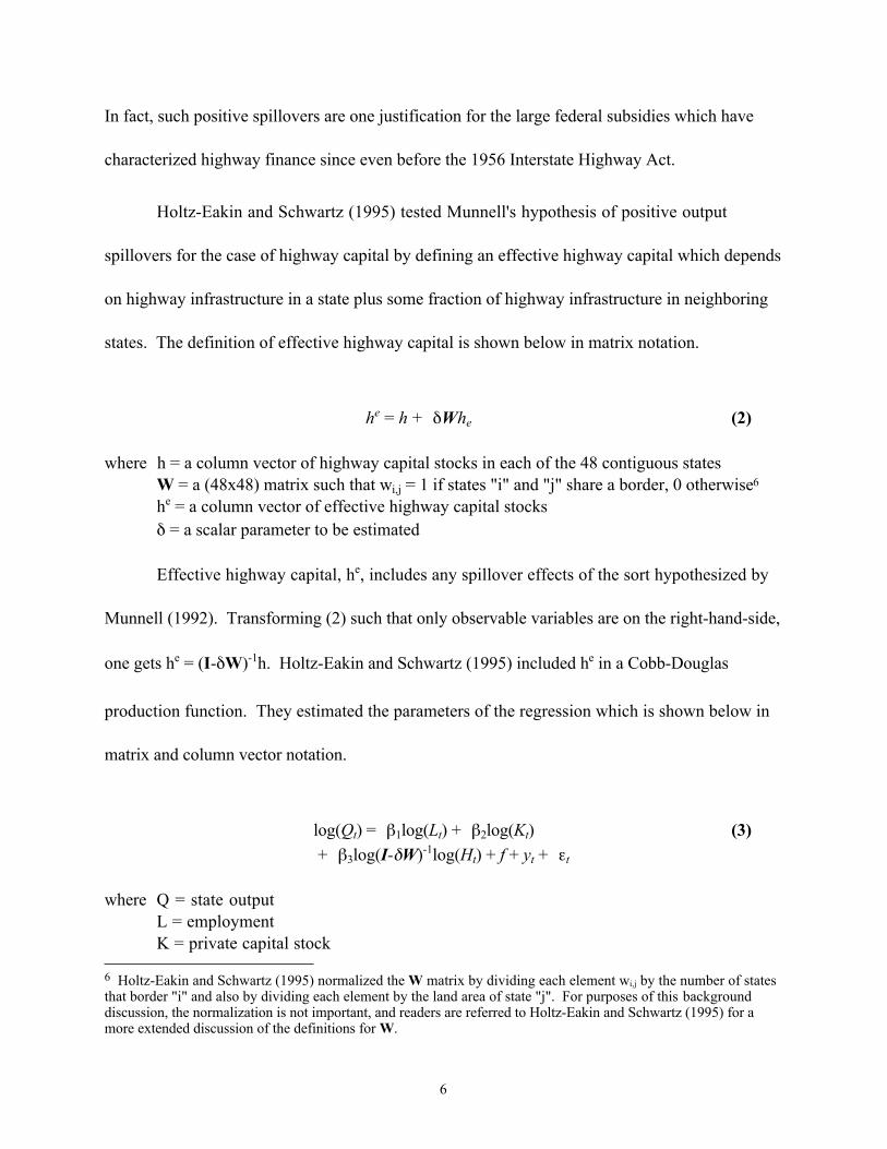
Holtz-Eakin and Schwartz (1995) tested Munnell's hypothesis of positive output

spillovers for the case of highway capital by defining an effective highway capital which depends

on highway infrastructure in a state plus some fraction of highway infrastructure in neighboring

states. The definition of effective highway capital is shown below in matrix notation.

he = h + dWhe (2)

where h = a column vector of highway capital stocks in each of the 48 contiguous statesW = a (48x48) matrix such that wi,j = 1 if states "i" and "j" share a border, 0 otherwise6

he = a column vector of effective highway capital stocksd = a scalar parameter to be estimated

Effective highway capital, he, includes any spillover effects of the sort hypothesized by

Munnell (1992). Transforming (2) such that only observable variables are on the right-hand-side,

one gets he = (I-dW)-1h. Holtz-Eakin and Schwartz (1995) included he in a Cobb-Douglas

production function. They estimated the parameters of the regression which is shown below in

matrix and column vector notation.

log(Qt) = b1log(Lt) + b2log(Kt) (3)+ b3log(I-dW)-1log(Ht) + f + yt + et

where Q = state outputL = employmentK = private capital stock

6 Holtz-Eakin and Schwartz (1995) normalized the W matrix by dividing each element wi,j by the number of statesthat border "i" and also by dividing each element by the land area of state "j". For purposes of this backgrounddiscussion, the normalization is not important, and readers are referred to Holtz-Eakin and Schwartz (1995) for amore extended discussion of the definitions for W.

7

H = state highway capital stockyt = year-specific interceptsf = a vector of time invariant state-specific variablese = an i.i.d. disturbance"t" indexes years

The coefficient d is a spillover parameter and thus measures the indirect effect of highway

capital in neighboring states. Holtz-Eakin and Schwartz (1995) rejected the hypothesis that

highway capital has positive output spillovers, and in some of their specifications the spillover

parameter was significantly negative.

Yet despite the fact that Holtz-Eakin and Schwartz (1995) rejected Munnell's (1992)

hypothesis, theoretically any indirect effect from highway capital is the net of two offsetting

effects -- the shift of economic activity discussed in, e.g., Forkenbrock and Foster (1990) and the

spillover economic benefits hypothesized by Munnell (1992). Given that, the sign of an indirect

effect depends on both the magnitude of the two offsetting effects and the geographic scale of the

data. This paper uses county data for California, providing considerably more geographic detail

than most previous production function research. The empirical work that follows tests both the

for the existence of direct and indirect economic effects from street and highway capital and for

the signs of those effects.

8

III. An Empirical Test

A. Background

For comparison with recent production function research, the empirical test is conducted

in the context of an aggregate production function. A county production function is modified to

include both the street and highway capital stock within each county, and the street and highway

capital stock in other counties, as shown below.

Q = f(L,K,H,Ho) (4)

where Q = county outputL = county employmentK = private capital stock in the countyH = street and highway capital stock in the countyHo = street and highway capital stock in other counties

As an example, if highways contribute to output partially by drawing output away from

other areas, the coefficient on H should be positive in a specification based on (4), while the

coefficient on Ho would be negative. The key is defining other counties (i.e. Ho) in a sensible

way. I follow Holtz-Eakin and Schwartz and define Ho as the sum of the street and highway

capital in neighboring counties. This assumes that street and highway capital redistributes

economic activity across county borders. While that is not the only possibility, it is intuitive,

allows some comparison to prior research, and is in the spirit of the discussion in Forkenbrock

and Foster (1990). Since the goal here is primarily to test the hypothesis that direct and indirect

9

economic effects exist, rather than to give an exhaustive examination of possible definitions of Ho,

the empirical test will examine indirect effects between neighbor counties.

B. Data

Data for California counties from 1969 through 1988 are used to estimate the parameters

of a log-linear form of (4). Specifically, data are available on gross county product, employment,

private sector capital stock, and street plus highway capital stocks. Gross county product is

derived by apportioning state product to counties based on total county personal income, which

is consistent with the methodology used by the Southern California Association of Governments

to estimate county product within their region. Private capital stock is constructed by

apportioning Munnell's estimates of California private capital to counties.7 The apportioning

methodology is the same as that used in Munnell (1990), which in turn follows Da Silva Costa,

Elson, and Martin (1987). Highway and street capital stock is constructed using a perpetual

inventory method based on annual highway and street expenditures, in each county, starting in

1957. Employment in each county is available from the Census Bureau's County Business

Patterns for each year. See Boarnet (1995, Appendix A) for a detailed description of the data

sources and the methods used to construct the county product, private capital, and highway and

street capital variables.

The transportation capital stock variables, H and Ho, include both state highway and local

street capital. This differs from Holtz-Eakin and Schwartz (1995), who included only state

7 I thank Douglas Holtz-Eakin and Alicia Munnell for providing the state private capital data.

10

highway capital, and it also differs from studies of highway corridors such as the work of

Forkenbrock and Foster (1990). The reasons for including all ground transportation

infrastructure are several. First, since the geographic scale of this study is considerably smaller

than that of Holtz-Eakin and Schwartz (1995), one cannot as easily assume that indirect effects

are due mostly to the provision of highway infrastructure. The possibility that cross-county

travel can be facilitated by local streets should also be allowed in the empirical specification.

Second, indirect effects need not be due strictly to cross-county travel. The productive benefits

of transportation capital could be due to facilitating within-county travel. Again, that suggests

that street capital should be included in the test. Third, the purpose here is to simply test the

hypothesis that indirect effects exist. Given empirical support for that hypothesis, it is an

appropriate topic for future work to examine how much of any direct and indirect effect can be

attributed to state highway stocks versus the amount due to local street and road infrastructure.

A preliminary analysis of the data revealed that in all but three counties output was larger

than the value of the stock of street and highway capital in 1988. The three counties where the

value of street and highway stocks exceeded output were all sparsely populated rural counties

which, due to their geographic size, had large transportation capital stocks but very little

economic activity.8 Since these counties are outliers when compared with the rest of the sample,

they were dropped from the analysis that follows.9 The empirical work that follows is based on

8 Those counties were Alpine, Mono, and Sierra. Mono spans a large portion of the Mohave Desert near theNevada border, while Alpine and Sierra are in sparsely populated areas of the Sierra mountains. In 1988, AlpineCounty had a population of 1,100, Mono County had 9,100 persons, and Sierra County had a population of 3,300.

9 The idea that Alpine, Mono, and Sierra counties are outliers is supported both by examining a plot of output peremployee versus street and highway capital per employee, and by a Chow test which suggests a structural break inthe parameters for the outliers when compared with the rest of the sample. The regression in equation (6), below,was fit on the 3 outlier counties and the other 55 counties. The Chow test statistic for parameter stability across the

11

panel data for the remaining 55 counties from 1969 through 1988. Descriptive statistics for the

data are shown in Table 1.

C. Estimation and Results

As mentioned earlier, past production function studies of states has established the

importance of controlling for unique state effects (Evans and Karras 1994; Garcia-Mila,

McGuire, and Porter 1996; Holtz-Eakin 1994; Kelejian and Robinson 1994). Assuming a log-

linear Cobb-Douglas specification for equation (4) gives the regression shown below.

log(Qc,t) = b1log(Lc,t) + b2log(Kc,t) + b3log(Hc,t) (5)+ b4log(Hoc,t

) + fc + yt + ec,t

where Q, L, K, H, and Ho are as defined in equation (4)f = a vector of county-specific variablesy = a vector of year-specific interceptse = an i.i.d. error term10

"c" indexes counties; "t" indexes years

two sub-samples is 19.36, which is distributed as F23,1114. The hypothesis of coefficient stability across the twogroups of counties is rejected at better than the 1% level. Given that, it is appropriate either to drop the three outliercounties or to parameterize or otherwise control for how those counties differ from the rest of the sample. In otherwork (Boarnet 1996), the outliers are included in the analysis by controlling for how those counties differ from therest of the sample. That is done by examining indirect effects across counties of similar population density and percapita income. The result from that research is consistent with the work presented here. Both techniques supportthe hypothesis of negative indirect street and highway effects.

10 One could also model a first order spatially correlated error. In matrix notation, this would assume that, for anyyear, e = rWe + u, with u being a classical spherical error term. Regressions were tested with W defined such thatwi,j = 1 if counties "i" and "j" border, 0 otherwise, which is the same W matrix that is used in the empirical workbelow. Specifying such a spatially autocorrelated error structure does not substantively change any of the regressionresults reported in this paper. Maximum likelihood estimates for the model with a first order spatially correlatederror are available upon request from the author.

12

Note that the variables fc control for any unique, time-invariant county characteristics

which affect output but which are not otherwise measured with the data. The dummy variables

yt allow for common time effects, and thus control for the macroeconomy.

For any county, "i", the variable Ho is implemented as Sjwi,jHj, where wi,j are weights.

The weights are defined such that wi,j equals one if counties "i" and "j" share a border; otherwise

wi,j equals zero. Thus for any county "i", the street plus highway capital in other counties (Ho)

is the sum of street plus highway capital in all counties that border "i".11 Given this definition

for Ho, the regression in equation (5) can be written in matrix notation as

log(Qt) = b1log(Lt) + b2log(Kt) + b3log(Ht) (6)+ b4log(WHt) + f + yt + et

where W = a (55x55) matrix with elements wi,j = 1 if counties "i" and "j" share a border,otherwise wi,j = 0t subscripts indicate yearsall variables are column vectors of observations for the 55 counties for a given year

The definition of Ho in equation (6) differs slightly from the one used by Holtz-Eakin and

Schwartz (1995). As mentioned earlier, they defined an effective highway capital equal to

(I-dW)-1H, where I is an identity matrix and W is a matrix that defines how states (in the case of

their study) neighbor each other. The Holtz-Eakin and Schwartz (1995) formulation allows

highway capital in one state to effect immediate neighbors in a "first-round effect", and then

effect the neighbors of those immediate neighbors in a "second-round" effect, and so on. The

11 While the idea of summing neighbors' street and highway capital is intuitive, one might also wish to take aweighted sum. One possibility is to weight the wi,j by the inverse of the number of neighbors, such that thevariable Ho is the average of street and highway capital in adjacent counties. Using that definition for Ho does notchange the results of any regressions reported in this paper.

13

parameter d measures how the neighbor relationship decays from the "first round" or immediate

neighbors, to neighbors of immediate neighbors, and so on. The use of the variable WH in

equation (6) restricts attention to only immediate (or "first round") neighbors.

Either definition can test for indirect effects from street and highway capital. Attention

here is restricted to first-round neighbor effects both because that allows a specification that is

linear in the parameters and because focusing only on immediate neighbors is a more conservative

test of indirect effects, since any higher order neighbor effects are not measured.

The unique county variables, fc, can either be treated as part of the intercept (fixed effects

estimation) or part of the error term (random effects estimation). Since random effects assumes

that the fc are part of the error term, that requires that the fc be orthogonal to the other

independent variables. The Hausman test statistic for fixed versus random effects for the

specification in equation (6) is 18.82, which follows a chi-squared distribution with four degrees

of freedom. At better than the 1% level, this rejects the hypothesis that the county effects are

orthogonal to the other independent variables, suggesting that fixed effects estimation should be

used.

Fixed effects coefficient estimates for (6) are shown in Table 2. The coefficients on all

four inputs are statistically significant at the 1% level. The coefficients on labor and private

capital are 0.62 and 0.20 respectively, which is consistent with the range of magnitudes obtained

in other production function studies (e.g. Aaron 1990; Garcia-Mila, McGuire, and Porter 1996;

Holtz-Eakin 1994). The coefficient on own street and highway capital (H) is significantly

positive, and the coefficient on neighbor counties' street and highway capital (WH) is

14

significantly negative. This supports the hypothesis of opposing direct and indirect economic

effects from transportation infrastructure, and suggests that some of the output increases

associated with street and highway capital are a redistribution of activity from neighboring

counties.

Garcia-Mila and McGuire (1992) and Munnell (1992) have both noted that fixed effects

estimation identifies parameters based on short-run year-to-year fluctuations in the data. As

such, the technique does not capture any long-run relationship between public capital and

output. To avoid this problem, Holtz-Eakin and Schwartz (1995) suggest transforming the

specification in (6) into what they call long differences.

Standard first differences specifications can be obtained by subtracting from the equation

for year "t" the equation for the previous year, "t-1". While that eliminates the time invariant

fixed effect (the fc), it still identifies parameters based only on short-term year-to-year

fluctuations. To overcome that problem, Holtz-Eakin and Schwartz suggest transforming the

data by differencing over several years. Adapting that approach, consider subtracting from the

equation for year "t" the equation for ten years earlier, "t-10". For example, subtract the equation

for 1969 from the equation for 1979. The differences are now ten year changes, which should be

sufficient to capture long-run relationships between county output, own county street and

highway capital, and neighbor counties' street and highway capital.12 Similarly, one could express

12 Research on lagged adjustment models of urban economies gives justification for using ten year differences.Carlino and Mills (1987) estimated a lagged adjustment model of population and employment growth in counties.They found that, for both county population and county employment, approximately 15% of the gap between actualand equilibrium values was closed in ten years. Grubb (1982) and Luce (1994) estimated similar models for cities.They found adjustment speeds which implied that the cities in their samples closed between 30% and 100% of thegap between actual and equilibrium values in ten years. These results suggest that ten years is a sufficient timeperiod to capture a reasonable amount of long run change.

15

equation (6) as the difference between 1980 and 1970 values. Given the available data, ten such

differenced specifications can be obtained -- the difference between 1969 and 1979, between 1970

and 1980, and so on up to and including the difference between 1978 and 1988 values.

Furthermore, given that the regression coefficients in (6) are assumed to be time invariant, one can

pool each of the ten equations. This gives an equation with 550 observations, with each

observation based on ten year differences in the levels of the variables.13

Expressing the data in differences rather than levels has the added advantage of

ameliorating any spurious correlations due to unit roots in the series. Previous analysis of

national time series data has suggested that the relationship between output and public capital

might be a spurious one due to common trends in the levels of the variables (Tatom 1991).

Statistical tests for such problems usually require longer time series than are available here.14

Given that, the most cautious approach is to estimate a differenced specification. Taking ten-

year differences transforms the specification into differences while preserving the long-run

relationship between the variables.

The results of estimating equation (6) in ten year differences, while pooling all

observations, are shown in Table 3. The results are essentially the same as in Table 2. The

coefficients on labor and private capital are significantly positive. The coefficient on own street

13 Note that pooling differences across ten different ten-year time periods avoids the serial correlation problemdiscussed in Holtz-Eakin and Schwartz (1995, p. 463).

14 Davidson and MacKinnon (1993, chapter 20) note that the small sample properties of tests for non-stationarityand spurious correlation rely on restrictive assumptions, including the assumption of serially uncorrelated errors inthe test regressions, which are not likely to hold in practice. Thus the tests are most reliable when the asymptoticproperties, which depend on the length of the time series, can be used.

16

and highway capital is significantly positive and the coefficient on neighbors' street and highway

capital is significantly negative, again suggesting opposing direct and indirect output effects.

Absent a full structural model, there are three reasons why the associations in Tables 2

and 3 more likely show the effect of street and highway infrastructure on output rather than the

reverse causal link. First, the fixed county effects control for any time invariant characteristics

which might cause more wealthy counties to either obtain more highway funding or spend more

local money on roads. Second, using the vector autoregression techniques described in Holtz-

Eakin, Newey, and Rosen (1986), changes in highway plus street capital stocks were regressed

on lagged changes of both highway plus street capital stocks and county output. The null

hypothesis that the coefficients on output equaled zero could not be rejected in regressions with

two, three, four, or five lags, suggesting that the primary channel of causality does not flow from

county output to highway capital stocks.15 Third, the indirect effect (the negative coefficient on

neighbor counties' street and highway capital) argues that causality is from transportation

infrastructure to output. That is consistent with transportation infrastructure investments which

shift economic activity from place to place. The reverse causal link, namely that higher county

output reduces street and highway infrastructure stocks in neighboring counties, does not have an

equally compelling explanation.

15 Only regressions with two, three, four, and five lags were tested. The test statistic follows a chi-squareddistribution. For five lags, the statistic is 0.0032 with 5 degrees of freedom. For four lags, the statistic is 0.0026with 4 degrees of freedom. For three lags, the statistic is 0.0039 with 3 degrees of freedom. For two lags, thestatistic is 0.0011 with 2 degrees of freedom.

17

Section IV: Interpretation

Given the magnitudes on own and neighbor county street and highway capital in Tables 2

and 3, one might be tempted to conclude that the direct and indirect effects are of equal and

opposing magnitude. Yet there are two reasons why one should be skeptical of such a

conclusion. First, note that there are several possible ways to define the wi,j. If the concern is to

measure correlation between particular neighbors, the magnitude of the non-zero elements of W is

not of vital importance. An argument based on coefficient magnitudes, on the other hand,

requires that the magnitudes of the weights be correct. Since it is difficult to determine a priori

the proper magnitudes for the wi,j, the cautious approach is not to read too much into the

magnitudes of the coefficients on own county and neighbor counties' street and highway capital.

Second, if transportation infrastructure is productive for counties (as the positive

coefficient on own county street and highway capital suggests), then theoretically the direct and

indirect effects ought not perfectly cancel. A contrived example can help clarify this point.

Suppose that a county, call it "A", gets an increase in transportation infrastructure. Further

suppose that the new infrastructure enhances the returns to private factors of production in

County A. Some firms might then move to County A from other counties in order to benefit

from the more productive environment in County A. Even if all increased output in A is due to

the production of firms which moved into the county, the direct effect of increased output in A

must be larger than the indirect effect of decreased output in the other counties where the migrant

firms were previously located. That's because each firm that moved into County A is more

productive, and thus can produce more output (given the same private inputs) than they could

18

have outside of A. After all, the increased productivity in County A is what caused the firms to

move in the first place.16

Overall, theory suggests that if street and highway capital is productive for counties, the

net of the direct and indirect effects ought to be greater than zero sum. Thus the results in this

work are in conflict with the recent state-level studies which found that public infrastructure,

transportation infrastructure included, is not productive (e.g. Evans and Karras 1994; Garcia-

Mila, McGuire, and Porter 1996; Holtz-Eakin 1994; Kelejian and Robinson 1994). It is not

likely that the difference in findings is due to econometric specification, since the specifications

used here adopt the same techniques used in the recent state-level studies.

While a full reconciliation of this work with the results from state studies is a topic for

future research, one possibility will be mentioned here. If the coefficient on public capital is

biased downward due to noisy data, it is possible that state studies give elasticities that are

insignificantly different from zero when public capital actually has a small marginal effect on

output or productivity. At the state level, the direct and indirect county effects partially cancel.

Thus the coefficient on state infrastructure is the net of any within-state direct and indirect

effects, and ought to be smaller that the direct (county) effect measured in this study.

Equivalently, with county data, the coefficient on own county transportation infrastructure

ought to be larger than comparable estimates from state studies. Given that, even with noisy

data, it might be possible to estimate statistically significant transportation infrastructure

16 For a more formal discussion of this, see Boarnet (1996).

19

elasticities with county data using techniques that do not yield significantly positive elasticities

with state data.

Section V: Policy Recommendations

Despite the fact that the evidence here is consistent with productive street and highway

capital, the recent skepticism about using public infrastructure as an engine of economic growth

(e.g. Holtz-Eakin 1993; Krol 1995) is well founded. Even if transportation infrastructure is

productive for counties (and a full reconciliation of this research with previous studies awaits

future work), policy-makers ought to be cognizant of the possibility of economic losses outside

the immediate project area. If studies of particular corridors measure only direct economic

effects, those studies might overestimate the total economic gains from a project, as Forkenbrock

and Foster (1990) suggested.

This raises the question of how to consider economic impacts in highway project

analysis. Determining the magnitude of even the direct (or nearby) economic impact has always

been difficult, since it is hard to control for the ceteris paribus condition of what would have

happened had the highway not been built. The lesson here is that determining economic impacts

is even more difficult than corridor studies or project analysis would suggest. Even if the ceteris

paribus condition can be enforced, one must account for both direct and indirect economic

effects.

This places a considerable burden on project analysis, both since it requires that the study

consider impacts in places remote from the project and because it might not be a priori obvious

20

where to look for indirect effects. While this paper gives evidence of indirect economic effects

across neighboring counties, other locational patterns are also possible. Overall, economic

impacts generated from project analyses that do not attempt to measure indirect effects must be

viewed with caution. Future research and practice should consider more carefully how to

measure both the direct and indirect economic effects of transportation infrastructure.

Until that is done, some caution is required when interpreting evidence of street or

highway economic benefits. Since most studies of transportation projects are only designed to

illuminate the direct, or nearby, effects, policy-makers should be aware that investments that

appear to bring economic gains might also generate economic losses in areas remote from the

project.

21

Bibliography

Aaron, Henry J. 1990. Discussion of "Why is Infrastructure Important?" In Is There aShortfall in Public Capital Investment?, Alicia H. Munnell, ed. Proceedings of FederalReserve Bank of Boston conference, June 1990.

Aschauer, David Alan. 1989. Is Public Expenditure Productive? Journal of MonetaryEconomics 23: 177-200.

Boarnet, Marlon G. 1995. Transportation Infrastructure, Economic Productivity, andGeographic Scale: Aggregate Growth versus Spatial Redistribution. University ofCalifornia Transportation Center working paper number 255. Berkeley, California:University of California Transportation Center.

Boarnet, Marlon G. 1996. Geography and Public Infrastructure. Department of Urban andRegional Planning working paper number 1996-38. Irvine, California: Department ofUrban and Regional Planning, University of California at Irvine.

Carlino, Gerald A and Edwin S. Mills. 1987. The Determinants of County Growth. Journal ofRegional Science 27: 39-54.

Case, Anne C., James R. Hines, Jr., and Harvey S. Rosen. 1993. Budget Spillovers and FiscalPolicy Interdependence: Evidence from the States. Journal of Public Economics 52: 285-307.

Dalton, Douglas F. 1991. Wisconsin's Corridors 2020: Highway Planning for EconomicVitality. ITE Journal, October, 1991, pp. 21-24.

Da Silva Costa, Jose, Richard W. Elson, and Randolph C. Martin. 1987. Public Capital,Regional Output, and Development: Some Empirical Evidence. Journal of RegionalScience 27: 419-437.

Davidson, Russell and James G. MacKinnon. 1993. Estimation and Inference in Econometrics.Oxford: Oxford University Press.

Duffy-Deno, Kevin T and Eberts, Randall W. 1991. Public Infrastructure and RegionalEconomic Development: A Simultaneous Equations Approach. Journal of UrbanEconomics 30: 329-343.

Eberts, Randall W. 1986. Estimating the Contribution of Urban Public Infrastructure to RegionalGrowth. Working Paper number 8610. Cleveland, Ohio: Federal Reserve Bank ofCleveland.

Eberts, Randall W. and Michael S. Fogarty. 1987. Estimating the Relationship Between LocalPublic and Private Investment. Working Paper number 8703. Cleveland, Ohio: FederalReserve Bank of Cleveland.

Evans and Karras. 1994. Are Government Activities Productive? Evidence from a Panel of U.S.States. Review of Economics and Statistics 76,1: 1-11.

22

Forkenbrock, David J. 1990. Putting Transportation and Economic Development intoPerspective. Transportation Research Record number 1274.

Forkenbrock, David J. and Norman S. J. Foster. 1990. Economic Benefits of a CorridorHighway Investment. Transportation Research A 24A,4: 303-312.

Forkenbrock, David J. and D. J. Plazah. 1986. Economic Development and State-LevelTransportation Policy. Transportation Quarterly 40,2: 143-157.

Garcia-Mila, Teresa and Therese J. McGuire. 1992. The Contribution of Publicly ProvidedInputs to States' Economies. Regional Science and Urban Economics 22: 229-241.

Garcia-Mila, Teresa, Therese J. McGuire, and Robert H. Porter. 1996. The Effect of PublicCapital in State-Level Production Functions Reconsidered. Review of Economics andStatistics forthcoming.

Gramlich, Edward M. 1994. Infrastructure Investment: A Review Essay. Journal of EconomicLiterature 32:1176-1196.

Grubb, W. Norton. 1982. The Dynamic Implications of the Tiebout Model: The ChangingComposition of Boston Communities, 1960-1970. Public Finance Quarterly 10: 17-38.

Holtz-Eakin, Douglas. 1993. Why a Federal Plan Isn't Needed. Spectrum -- The Journal of StateGovernment 66,4: 35-44.

Holtz-Eakin, Douglas. 1994. Public-Sector Capital and the Productivity Puzzle. Review ofEconomics and Statistics 76,1: 12-21.

Holtz-Eakin, Douglas, Whitney Newey, and Harvey S. Rosen. 1988. Estimating VectorAutoregressions with Panel Data. Econometrica 56: 1371-1395.

Holtz-Eakin, Douglas and Amy Ellen Schwartz. 1995. Spatial Productivity Spillovers fromPublic Infrastructure: Evidence from State Highways. International Tax and PublicFinance, forthcoming.

Jorgenson, Dale W. 1991. Fragile Statistical Foundations: The Macroeconomics of PublicInfrastructure Investment. Conference Paper, American Enterprise Institute, February,1991.

Kelejian, Harry H. and Dennis P. Robinson. 1994. Infrastructure Productivity: A Razor's Edge.Working Paper, University of Maryland.

Krol, Robert. 1995. Public Infrastructure and State Economic Development. EconomicDevelopment Quarterly 9: 331-338.

Lemer, Andrew C. 1992. We Cannot Afford Not to Have a National Infrastructure Policy.Journal of the American Planning Association 58,3: 362-367.

Luce, Thomas F., Jr. 1994. Local Taxes, Public Services, and the Intrametropolitan Location ofFirms and Households. Public Finance Quarterly 22,2: 139-167.

23

McGuire, Therese J. 1992. Highways and Macroeconomic Productivity, Phase Two. Report toU.S. Department of Transportation. Chicago, Illinois: School of Urban Planning andPolicy, University of Illinois at Chicago.

Mohring, Herbert and Mitchell Harwitz. 1962. Highway Benefits: An Analytical Framework.Evanston, Illinois: Northwestern University Press.

Munnell, Alicia H. 1990. How Does Infrastructure Affect Regional Economic Performance? InIs There a Shortfall in Public Capital Investment?, Alicia H. Munnell, ed. Proceedings ofFederal Reserve Bank of Boston conference, June 1990.

Munnell, Alicia H. 1992. Policy Watch: Infrastructure Investment and Economic Growth.Journal of Economic Perspectives 6,4: 189-198.

Nathan, Richard P. 1992. Needed: A Marshall Plan for Ourselves. In Exploring UrbanAmerica: An Introductory Reader, Roger W. Caves, ed. Thousand Oaks, California: SagePublications.

Seskin, Samuel N. 1990. Comprehensive Framework for Highway Economic ImpactAssessment: Methods and Results. Transportation Research Record number 1274.

Tatom, John A. 1991. Public Capital and Private Sector Performance. St. Louis Federal ReserveBank Review 73,3: 3-15.

U.S. Department of Transportation. 1992. Assessing the Relationship Between TransportationInfrastructure and Productivity. Policy Discussion Series number 4. Washington, D.C.:U.S. Department of Transportation.

24

Table 1: Descriptive Statistics

Variable Mean StandardDeviation

Minimum Maximum

LevelsQ: County Output 7.38 1.68 4.16 11.98L: Employment 10.09 1.83 6.68 15.10K: Private Capital 7.07 1.59 3.86 11.63H: Own County Street andHighway Capital

5.87 1.13 4.02 9.54

WH: Neighbor Counties' Street andHighway Capital

7.68 0.90 5.84 9.94

Ten Year DifferencesQ: County Output 0.40 0.22 -0.66 1.16L: Employment 0.47 0.20 -0.13 1.10K: Private Capital 0.43 0.24 -0.63 1.29H: Own County Street andHighway Capital

0.13 0.12 -0.15 0.51

WH: Neighbor Counties' Street andHighway Capital

0.13 0.08 -0.04 0.40

Note: Output, private capital, and street and highway capital are in logs of millions of dollars.Employment is in logs.

25

Table 2: Fixed Effects Regression ResultsDependent Variable = log(county output)

independent variableLabor (L) 0.62

(0.025)Private Capital (K) 0.20

(0.020)Own County Street and HighwayCapital (H)

0.16(0.040)

Neighbor Counties' Street andHighway Capital (WH)

-0.21(0.059)

Note: All variables are in logs. Standard errors are in parentheses below coefficients.Coefficients on year dummy variables not shown. Number of observations = 1100.

26

Table 3: Regression Results, Ten Year DifferencesDependent Variable = log(county output)

independent variableLabor (L) 0.69

(0.036)Private Capital (K) 0.18

(0.030)Own County Street and HighwayCapital (H)

0.22(0.056)

Neighbor Counties' Street andHighway Capital (WH)

-0.23(0.08)

Note: All variables are ten-year differences of logs. Standard errors are in parentheses belowcoefficients. Coefficients on year dummy variables not shown. Number of observations = 550.