the development of an accuracy of a doppler …

THE DEVELOPMENT OF AN ACCURACY OF A DOPPLER GLOBAL

SYSTEM FOR ONE DIMENSIONAL VELOCITY MEASUREMENT

A Thesis

by

MUSTAFA KARABACAK

Submitted to the Office of Graduate and Professional Studies of

Texas A&M University

in partial fulfillment of the requirements for the degree of

MASTER OF SCIENCE

Chair of Committee, Gerald Morrison

Committee Members, Devesh Ranjan

Yassin A. Hassan

Head of Department, Andreas Polycarpou

August 2014

Major Subject: Mechanical Engineering

Copyright 2014 Mustafa Karabacak

ii

ABSTRACT

The development of a Doppler Global System for one dimensional velocity

measurement including both hardware and software development is described. The

Doppler Global Velocimetry (DGV) system is a whole field measurement system based

on Doppler shifting of the light frequency reflected by seeded particles or rotating disc

surface speed. The relationship between the Doppler shift and the transmission ratio is a

key part of the DGV system to calculate measured velocity. The absorption line filter is

a device to determine the Doppler shift by converting a frequency to an intensity.

This study describes the optical system and software developments to increase

the accuracy of the DGV system. The new light source and two charged coupled device

cameras are the main hardware developments. A LabView code was created to calibrate

the ALF cell automatically as a software development.

The DGV system spatial and intensity calibration was completed for accurate

measurement, and the ALF cell was calibrated to maintain the relationship between the

transmission ratio and frequency shift of the laser. The system was tested by measuring

the surface speed across a 99.06 mm white painted disc at 18000 and 10020 rpm when

the transmission ratios of the ALF cell are 1.1, 0.5 and 0.085.

As a result, the error of the system was -8 to 12 m/s when the transmission ratio

was 1.1. The measured velocity had ±5 m/s when the transmission ratio was 0.5.

However, the error was significantly high at the bottom right and top left part of the disc

because these regions did not receive enough light. Also, the measurement was not

iii

accurate when the transmission ratio was 0.08. The change of transmission ratio was

almost constant when the transmission ratio was 0.08, so Doppler shift calculation was

not calculated accurately because of that reason.

In conclusion, the rotating disc horizontal surface speed was measured at

different rotational speeds and transmission ratios. Results prove that new two Dalsa

Pantera TF 1M30 cameras and, Oxxius continuous wave diode pumped solid state laser

as a light source work properly to measure velocity in our DGV system.

iv

DEDICATION

This work is dedicated to my family and fiancé who supported me through my

time at Texas A&M University.

v

ACKNOWLEDGEMENTS

I would like to thank Dr. G. L. Morrison for his guidance and support throughout

my research. I would also like to thank to my committee members, Dr. Devesh Ranjan

and Dr. Yassin A. Hassan.

I would like to thank my friend at the Turbolab, especially Sahand Pirouzpanah,

Scott, Yusuf and Burak for giving me advice and helping me finish my research.

I would like to thank my roommates, Abdulkadir and Gokhan for their support.

I also would like to thank BOTAS for financial support throughout my master

education.

vi

TABLE OF CONTENTS

Page

ABSTRACT ....................................................................................................................... ii

DEDICATION .................................................................................................................. iv

ACKNOWLEDGEMENTS ............................................................................................... v

TABLE OF CONTENTS .................................................................................................. vi

LIST OF FIGURES......................................................................................................... viii

1. INTRODUCTION.......................................................................................................... 1

2. PRINCIPLE OF OPERATION ...................................................................................... 3

3. LITERATURE REVIEW ............................................................................................... 8

4. OBJECTIVES .............................................................................................................. 17

5. EXPERIMENTAL APPARATUS ............................................................................... 18

5.1 Light Source ........................................................................................................... 18

5.2 Temperature Controller .......................................................................................... 20

5.3 Power Meters.......................................................................................................... 21

5.4 Doppler Image Analyzer Unit ................................................................................ 22

5.5 Charged Coupled Device Camera .......................................................................... 26

5.6 Velocity Calibration Device ................................................................................... 28

5.7 Data Acquisition ..................................................................................................... 30

6. IMAGE PROCESSING TECHNIQUE ....................................................................... 33

6.1 Spatial Calibration .................................................................................................. 33

6.2 Centroid Estimation................................................................................................ 34

6.3 Intensity Calibration ............................................................................................... 40

7. RESULT AND DISCUSSION .................................................................................... 46

7.1 Laser Stability ........................................................................................................ 46

vii

7.2 Absorption Line Filter Calibration ......................................................................... 47

7.3 Image Analyses Method ......................................................................................... 51

7.4 Rotating Disc Measurement ................................................................................... 52

7.4.1 Disc Speed Measurement at 18420 rpm and 1.1 Transmission Ratio ............. 54



7.4.4 Disc Speed Measurement at 18000 rpm and 0.08 Transmission Ratio ........... 74

8. CONCLUSION AND RECOMMENDATIONS ......................................................... 79

8.1 Conclusion .............................................................................................................. 79 8.2 Recommendations .................................................................................................. 81

REFERENCES ................................................................................................................. 83

viii

LIST OF FIGURES

Page

Figure 1 Determination of measured velocity components direction based on laser

propagation and receiver location. ....................................................................... 3

Figure 2 Transmission curve vs. frequency of laser light .................................................. 4

Figure 3 Global Doppler shift in laser light sheet .............................................................. 6

Figure 4 Optical schematic of Doppler image analyzer ..................................................... 7

Figure 5 Light source of the DGV system Oxxius 532-S-COL-PP ................................. 20

Figure 6 TC-200 THORLABS temperature controllers ................................................... 21

Figure 7 PM100A power meter ........................................................................................ 22

Figure 8 Edmund optics techspec 0.16X TML telecentric lens ....................................... 25

Figure 9 CQ19100-I quartz reference cell with power meter sensors and heater

rings.................................................................................................................... 25

Figure 10 Two CCD cameras and ALF cell ..................................................................... 27

Figure 11 Aluminum sheet in which image analyzer unit was located ............................ 27

Figure 12 3.9 inch diameter rotating disc ......................................................................... 28

Figure 13 ALF cell frequency shift vs transmission ratio curve with three

transmission ratio range that were used for the measurement ......................... 29

Figure 14 Front panel of the LabView program for the ALF cell calibration.................. 31

Figure 15 Filtered images for spatial calibration ............................................................. 35

Figure 16 Unfiltered images for spatial calibration ......................................................... 35

Figure 17 Unfiltered image pixel location of dots ........................................................... 37

ix

Figure 18 Filtered image pixel location of dots ............................................................... 37

Figure 19 Unfiltered image physical location of each dot ............................................... 38

Figure 20 Filtered image physical location of each dot ................................................... 38

Figure 21 Filtered image calculated and known dots locations ....................................... 39

Figure 22 Unfiltered image calculated and known dots locations ................................... 40

Figure 23 Example of linear fit relating to ‘lumens’ for filtered image ........................... 41

Figure 24 Example of linear fit relating intensity to ‘lumens’ ......................................... 42

Figure 25 Result from intensity calibration 1024x1024 slope relationship along the

filtered camera ................................................................................................. 43


unfiltered camera ............................................................................................. 43

Figure 27 Result from intensity calibration 1024x1024 intercept relationship along the

filtered camera ................................................................................................. 44

Figure 28 Result from intensity calibration 1024x1024 intercept relationship along the

unfiltered camera ............................................................................................. 45

Figure 29 Table of the ALF transmission ratio vs frequency .......................................... 50

Figure 30 Filtered image of the disc at 0 rpm and 1.1 transmission ratio ........................ 54

Figure 31 Unfiltered image of the disc at 0 rpm and 1.1 transmission ratio .................... 55

Figure 32 Lumen value of the unfiltered image at 18420 rpm and 1.1 transmission

ratio .................................................................................................................. 55

Figure 33 Lumen value of the filtered image at 18420 rpm and 1.1 transmission

ratio .................................................................................................................. 56

Figure 34 Transmission ratio of the disc at 18420 rpm and 1.1 transmission ratio ......... 58

Figure 35 Frequency change at 18420 rpm and 1.1 transmission ratio (GHz) ................ 58

Figure 36 Rotating disc frequency shift at 18420 rpm and 1.1 transmission ratio

(GHz) ............................................................................................................... 59

x

Figure 37 Speed of the rotating disc (m/s) at 18420 rpm and 1.1 transmission ratio....... 59

Figure 38 Error of the measured velocity (m/s) at 18420 rpm and 1.1 transmission

ratio .................................................................................................................. 60

Figure 39 Filtered image of the disc at 0 rpm and 0.5 transmission ratio ........................ 61

Figure 40 Unfiltered image of the disc at 0 rpm and 0.5 transmission ratio .................... 62


ratio .................................................................................................................. 62

Figure 42 Lumen value of the unfiltered Image at 17820 rpm and 0.5 transmission

ratio .................................................................................................................. 63




(GHz) ............................................................................................................... 66



ratio .................................................................................................................. 68


ratio .................................................................................................................. 69


ratio .................................................................................................................. 69




(GHz) ............................................................................................................... 72


xi


ratio .................................................................................................................. 73

Figure 55 Unfiltered image lumen ratio at 18000 rpm and 0.08 transmission ratio ........ 75

Figure 56 Filtered image lumen ratio at 18000 rpm and 0.08 transmission ratio ............ 75

Figure 57 Transmission ratio of the disc at 18000 rpm and 0.08 transmission ratio ....... 76

Figure 58 Frequency change on the disc at 18000 rpm and 0.08 transmission ratio ....... 77

Figure 59 Frequency shift of the disc at 18000 rpm and 0.08 transmission ratio ............ 77

Figure 60 Speed of the disc at 18000 rpm and 0.08 transmission ratio ........................... 78

1

1. INTRODUCTION

Laser Doppler Velocimetry (LDV), Particle Image Velocimetry (PIV), and

Doppler Global Velocimetry (DGV) are types of nonintrusive laser based anemometry.

A DGV can measure an unsteady flow field and it is able to supply these data in real

time. DGV is able to simultaneously measure global three dimensional velocity of a

seeded flow field by measuring the Doppler shift in light reflected from seed particles in

the flow.

LDV uses two laser beams focused onto a desired point and measures the

frequency of the difference between the Doppler shifts of a light reflected from seed

particles. The system operates on a point by point basis, so it is time consuming to obtain

an entire flow field.

PIV is the most common global technique used to measure a velocity field. PIV

uses a pulsed laser light sheet to illuminate a seeded flow and a camera to record images.

When flows are seeded, the cameras take pictures at known times and measures the

distance traveled by the seed. PIV can measure simultaneously over the area that the

cameras views. The system depends on imaging of travelling individual seeded particles

and requires a mathematic algorithm to track particles and measure velocity. PIV is less

accurate than LDV techniques in complicated flow fields. Particles that are

2

perpendicular to the light sheet produce errors in the system since their velocity must be

low enough to not transit the sheet of light during a two picture sequence.

Michelson interferometry is capable of producing a three dimensional Doppler

image of a global flow field. Fringe patterns are used to measure a constant phase shift

of the Doppler shifted light with this system. The Michelson interferometry can produce

three dimensional Doppler images but it is difficult to arrange the optics and difficult to

process the resulting fringe images.

The DGV system offers an economic and quicker global measurement when it is

compared with other global measurement techniques. The DGV system uses a narrow

frequency laser and a notch filter to measure a Doppler shift across the field of view.

However, small Doppler shifts are difficult to resolve in high flow speed, and this is the

major disadvantage of the system.

3

2. PRINCIPLE OF OPERATION

An LDV system was developed by Yeh and Cummins [1], and the optical

arrangement of the LDV system has been modified for the DGV. A Schematic diagram

of the DGV system and how to determine a measured velocity component vector is

shown Figure 1. Measuring a Doppler shift frequency of a laser light and relating it with

a velocity of fluid is a main principle of the DGV system. An absorption line filter

(ALF) was developed and patented by Komine [2] in 1990. This special absorption line

filter contains molecules which absorb light near a certain laser frequency. A diode

pumped solid state continuous wave laser frequency is 5.6×1014 Hz (532 nm) is one of

these. The properties of molecular iodine in the ALF cell can produce an absorption line

as presented in Figure 2.

Figure 1 Determination of measured velocity components direction based on laser

propagation and receiver location.

4

Figure 2 Transmission curve vs. frequency of laser light

The laser frequency must be stable, monochromatic, and have a much narrower

bandwidth than the width of absorption line filter. The laser frequency νo is tuned to a

midpoint of the one side of the u shape filter, and when the absorption changes

approximately linear with the frequency changes. The ALF filter absorption is 50% at

this frequency, so if the object or the particle moves, the transmission ratio will change

depend on the positive or negative velocity. For the system developed, the laser light

was separated into two beams by a beam splitter. Two power meters, and an ALF cell

were used to measure the transmission ratio of the ALF cell by measuring the power of

the laser light that is filtered and an unfiltered. Also, a temperature controller was used to

heat ALF cell and keep the ALF cell in stable temperature since the cells response is

temperature dependent. This system allows us to be able to measure the frequency drift

of the laser, and the transmission ratio of the ALF cell. If the measured Doppler shifted

5

frequency is higher than νo, it indicates positive velocities by resulting in an increased

transmission. If the Doppler shifted frequency is lower than νo, it indicates negative

velocity by resulting a decreased transmission. The relation of the transmission to the

frequency can be reversed by tuning the laser to a lower frequency side of the absorption

profile. This change in the transmission is proportional to the Doppler frequency shift of

the scattered light that is produced by the particle’s motion along the measurement

vector shown in Figure 1. The governing equation is given by:

∆𝑣 = 𝑣0(�̂� − 𝑙)̂ ∙�⃗⃗�

𝑐

where ∆𝑣 is the Doppler frequency shift, �̂� and 𝑙 are the unit vectors in the scattering and

laser light propagation directions respectively. �⃗� is the velocity vector of the moving

particle or object, 𝑣0 is the laser light frequency, and 𝑐 is the speed of light. A DGV

system can measure a one velocity component for given optical geometry. For three-

dimensional velocity measurements, three different observation directions (�̂�) or three

different laser beams oriented in three different directions (𝑙) need to be used.

The DGV system is a global measurements device thanks to the large diameter of

the ALF cell. The laser beam is expanded into a sheet of light with a lot of particles

providing the Doppler shifts in the DGV system, and this light intensity is collected by a

camera instead of a point detector that is used in the LDV system, so this makes the

DGV system a global device. The images that are captured simultaneously by a camera

yield intensity levels at each pixel whose relationship is a function of the velocity via

equation (1) and the relation:

Icamera(x,y,z)=IDoppler(x,y,z, ∆𝑣)·Tf(∆𝑣)

6

where IDoppler is an intensity due to the Doppler shifted light, Tf is a transfer function of

the ALF cell, and Icamera is an intensity of each pixel on the images. Figure 3 shows this

arrangement and the vector nature of the DGV.

Figure 3 Global Doppler shift in laser light sheet

The CCD video cameras are the observer unit of the Doppler Global Velocimetry

system. The seed density, the seed size, and the laser light sheet illumination are not

necessarily uniform, and this variations are not associated with the optical attenuations in

the iodine vapor induced by velocity. The unfiltered image is required to compensate for

these effects. The unfiltered image is separated from the filtered image by using a mirror

and a beam splitter, and the unfiltered image can be recorded separately by a second

camera. The unfiltered and filtered images are recorded simultaneously, and stored in a

7

computer. Figure 4 shows an optical arrangement of the unfiltered and filtered camera.

The filtered and unfiltered images are divided to correspond to the velocity caused

variations in the illuminated flow field.

Figure 4 Optical schematic of Doppler image analyzer

8

3. LITERATURE REVIEW

Doppler Global Velocimetry was developed and patented by H. Komine working

at the Northrop Corporation. A line filter, cameras and a laser were parts of the device.

An absorption line filter that was positioned in front of one camera and used to

determine velocity components by obtaining the Doppler shift of the laser light image

scattered from a seeded flow field. ALF and laser light were tuned 50% while

measurement processed, and two images were recorded to quantify intensity differences

versus velocity range. An Argon-ion laser was used in this experiment, and Komine

showed that a ±150 m/s velocity component can be obtained with 2 m/s resolution [2].

Meyers and Komine developed a one component DGV system with signal

processing electronics. A 5.25 inch floppy disc that was rotating up to 18500 rpm was

used to measure velocity, and a subsonic jet velocity, which was seeded with a fogger,

were measured. These results were compared with five holes probe and fringe-type laser

velocimeter, and showed that a DGV system has potential to measure velocity of flow,

and a capable to resolve velocity surges in the vortex flow field [3].

Meyers measured a 75 degree delta wing with a DGV system, and the results

were compared with previous measurement which was taken by a fringe-type laser

velocimeter and five-hole probe. Meyers indicated that influence of a particle size, a

number density, and a laser light sheet intensity errors were minimized by using

9

unfiltered images. Results showed that near vortex core velocity was almost the same

with previous results, but near edges of vortices velocity results were not what they

should be [4].

Meyers developed an optical technique to eliminate a signal processing step and

measure three dimensional velocity of above 75 degree delta wing flow. Meyers clarified

that exact overlay for signal and reference images were not provided by just physical

alignment of cameras. Factors which cause this inability were mismatched depths of

field, imperfections in the beam splitter, mirrors, ALF and no uniformity of pixel

distribution. A new image processing technique was developed to overcome this

problem. Dot paper was used to align both cameras and, centroid position of each grid

point was moved from its imaged position to its ideal position [5].

Meyers changed the flow condition from incompressible to Mach 2.8 and

measurement distance from 1 to 15m. A 75 degree delta wing velocity was measured

and compared new results with old results after improvement of image processing

technique. Also, an additional laser frequency monitoring system was used in a system

to monitor any laser drift during measurement [6].

Ford and Tatam used a digital image acquisition system by using CCD cameras

based on Komine patented DGV system. CCD cameras were used a first time in a DGV

system. They changed the geometry of the optical arrangement to see how it affects

errors of a system. Also, velocity resolution was restrained by uncooled camera because

of the camera noise in DGV. Calculations showed that error of the system due to angular

10

position across flow field is on the order of the resolution of the system when the angle

reaches 5 degree on side of center and 10 degrees of incident beam angle [7].

Smith used pulsed a Nd:YAG laser operating at 30 HZ , optically thin filter and

single CCD camera to reduce complexity of experiment. Most important part of this

experiment was single camera which was used as an observer instead of two cameras to

measure one component velocity. This was achieved by using splitters to place signal

and reference images side by side on the same camera. Advantages of the single camera

are not only economic and experimentally simple, but also that signal and reference

images are shown from exactly the same angle, which eliminates Mie scattering lobes

that affect the intensity ratio. Three different experiments were done by

changes/improvements in the imaging portion of an apparatus. Pressure matched sonic

jet and over expanded supersonic jet applied for these experiments, and each jet was

seeded with humidified supply air to generate fog. Smith realized that the biggest portion

of errors come from laser speckle. A pulsed laser causes laser speckle error, and using

the lowest possible f-number is a simple way to minimize speckle error. Another error

which was obtained is laser frequency locking, so during measurement frequency of the

laser should be monitored to catch any laser frequency drift [8].

M. Smith mentioned the biggest part of the random error is laser speckle when

using pulsed laser in DGV, and how to minimize this error. A frequency doubled

Nd:YAG laser and a He-Ne laser beam were used in this experiment. M. Smith

recommended that using lowest possible f-number, and large particles as a seed particle

to minimize laser speckle error. Detailed recommendations can be found in the paper [9].

11

McKenzie also used a Nd:YAG pulsed laser and a single high quality scientific

grade CCD camera for each velocity component in his experiment. He showed that using

a single high quality camera is better than using two averages quality cameras, and using

scientific grade cooled slow scan cameras increase capabilities of photometric device

because of it has low noise and high sensitivity. Other cameras have a greater noise

portion when compare with CCD camera. A single camera used by adjusting mirrors to

record reference and signal images in one camera, and using single camera reduce cost

of one more extra camera for one dimension [10].

McKenzie measured a rotating wheel speed to determine the low speed accuracy

of the DGV system by using a frequency doubled, injection seeded Nd:YAG laser. 15.2

cm iodine filter was used in his setup, and this filter is longer than any other filters which

were used in DGV system. Longer filter reduce thermal gradient effect of filter, but field

of view decrease and this is disadvantage of long filter. A polarized beam splitter was

used to minimize polarization effect and possible small f-number used to minimize laser

speckle error as Smith mentioned. Spatial calibration of the system performed on same

location for a measurement would take with same apparatus by using cameras. The

author indicates that 3×3 binning processed to reduce mapping and sampling errors of

images that were taken. Results showed that velocity below 2 m/s can be measured in

this experiment [11].

Morrison, Gaharan and DeOtte developed one component DGV system in Texas

A&M University, and they described problems and pitfalls they faced when processing.

They followed the same principle that was followed by Komine and Meyers. Cameras

12

which were used in this system had gain settings problem. The cameras must operate

fixed gain, but two cameras gain settings change independently, and that made invalid

light frequency to light intensity calibration to measure velocity field. Also, the cameras

light intensity were not uniform for each pixel, so a green lens that allows just green

light pass through the lens was used to overcome this problem. Lenses and a polarization

effect were other problems which were described in this paper. The intensity level of

each reference and signal images need to be kept nearly same, so neutral density (ND)

filters used to do that. In conclusion, inaccuracies obtained because of the system

apparatus performance, so they recommended necessary settings for cameras, lenses,

beam splitter and iodine filter cell to minimize inaccuracies [12].

Roehl used a three dimensional DGV system to measure velocity of a fuel spray

nozzle and the wake region of a car. The author mentioned laser stabilization is

extremely important to measure velocity and 2.7 MHz drift is equal 1 m/s uncertainty

when the light sheet and measured component angle is under 90 degree, so laser

stabilization and a monitoring system were used to stabilize the laser and reduce velocity

errors less than 0.5 m/s caused by laser drift. The three-dimensional velocity

measurement system can be setup by using two alternative methods. First, using one

light sheet and three synchronized cameras in different positions to measure three

dimension. One camera and three light sheets with different orientations were used to

measure three dimensions as a second method. A nonpolarized beam splitter was used to

minimize polarization effect and 12 bit CCD cameras were used as an observer. Image

processing technique applied to measure velocity simultaneously, and the whole process

13

took 30 second after images were recorded, so Roehl emphasized that DGV as good way

to measure a flow field quick and a very practical technique thanks to less required

processing and analyzing time [13].

Muller et al used a three dimensional DGV system to measure flow in pipes.

Three light sheets with different orientations and one camera system were used.

Reflected mirrors were used and adjusted to record the flow in pipe. Three dimensional

DGV data were compared with LDA, and result showed that deviations of DGV data

were relatively high, so DGV system must be further developed and optimized for

accurate measurement. However, this experiment showed that DGV system were

capable of measuring three dimensional velocity field in relatively short time when

compared with LDA, and this is the main advantage of DGV system [14].

Nobes, Ford and Tatam used fibre bundles for three dimensional velocity

measurement. Their setup was capable of measuring three components by using two

cameras and a single absorption line filter. One cell calibration was required instead of

multiple cell calibration, and that was an advantage of using multiple bundles for three

dimensional measurement. Three light sheet directions were needed to be define to

measure the three dimensional velocity field and fibre imaging bundles were set

according to these directions. They also used a fourth fibre bundle to monitor laser

frequency change and allow correction for any frequency movement of the laser while

measurement. 200 mm white painted rotating disc used to calibrate system, and disc was

perpendicular to laser. After calibration 70 mm diameter uniform seeded pipe nozzle jet

with 30 m/s exit velocity was measured [15].

14

Willert et al compared two previous three dimensional systems and LDA

measurements. Two parallel DGV systems which were applied in wind tunnel

performance, and used to measure reproducible tip vortex flow field generated by blunt

tip of an airfoil was chosen for this measurement. Both lasers were continuous wave and

the frequencies of the lasers were monitored. The agreement between various techniques

was 2 m/s, and DGV underestimate local velocity gradients. Willert showed that fibre

bundle system was able to accomplish this in one third the acquisition time [16].

Two pulsed Nd:YAG lasers were used in a two color DGV technique and applied

to free-jet by Arnette et al. Red light laser from a Nd:YAG pumped dye laser at 618 nm,

and green light laser was Nd:YAG frequency doubled laser at 532 nm. Laser beams

overlapped and created a sheet of light and scattered light was passed through an iodine

cell and recorded on CCD cameras. The green laser was tuned and used for frequency

shift, the red laser light intensity was not dependent to frequency change. The advantage

of the system is single camera is enough for one dimensional measurement. Even though

the system needed one more laser for one dimensional measurement, this is more

economical than two cameras system because camera price is more than laser price.

Also, one camera means simple data acquisition and no need spatial calibration. Problem

of the system was seed particle size because Rayleigh limit and the ratio of red and green

scattering signals depends on particle size, so seed particle size was increased [17].

Willert combined PIV and DGV systems to measure velocity of a single sector

combustor rig at pressures of 2 and 10 bars. Three components of the velocity and how

to create volumetric map of velocity were explained. Three different laser sheets were

15

used and stereoscopic measurement was done to create velocity volume. Seeded

particles were alumina particles to overcome seeded particle problem in combustor.

Results showed that DGV measurement uncertainty was about 1.5 m/s because of the

noise in frequency shift images, and PIV uncertainty was about 0.3 m/s for average of

100 images [18].

The main goal of Chain et al paper is influencing factors of absorption filters and

how it can be optimized during construction. As mentioned early, absorption filter is

dependent on the frequency of the laser light and velocity. Absorption profile from 0 to

100% is not achieved, so that affects the limitation of DGV and absorption line is not

steep enough to measure small velocity differences. Because of that reason, DGV is a

good technique to measure high speed flows. Also, Chan mentioned seven factors to

optimize absorption filter, purity of iodine, maintaining purity of iodine during filling

and degassing of filter, absorption cell materials and how it construct, control of cell

performance, relationship between dimensions and operating conditions of filter, and

windows and temperature control. Optimum filter can be constructed by following this

guideline [19].

Miles et al used sharp cut off molecular absorption filter to measure velocity in

Rayleigh scattering images of gas flows. Background scattering from walls and windows

is difficult to eliminate, so this scattering is main problem when boundary flow field is to

be measured. Sharp cut-off filter might be used to avoid background scattering problem

comes from walls and windows. Scattering signal was too low without seed particle, so

high power is laser needed to operate to collect enough scatted light. Velocity and

16

temperature can be measured from density of air that is related with intensity of scattered

light [20].

Naylor and Kuhlman setup a two dimensional velocity measurement DGV

system. Iodine vapor cell was used as a frequency discriminator to determine flow field.

Rotating wheel velocity measured to determine accuracy of DGV system. CCD cameras

were observer, and these cameras can reduce noise but increase cost of system. Laser

frequency was not controlled, but iodine cell used to determine any laser frequency drift.

High f-number lenses were used, because of that speckle noise increased, but incoming

light amount decreased. Some calibration methods were applied to align spatial and

intensity calibration of images, this calibration method can be found in paper. The RMS

value was found ±1.1 m/s for Y image direction, and ±0.9 m/s for X images direction. 8

bit limitation of imaging system and inaccuracies of cell calibration was defined as a

common source of errors [21].

17

4. OBJECTIVES

The primary objective of this study is increasing the accuracy of a one

dimensional DGV system, which was developed by Prof. Morrison and Dr. Gaharan. A

second objective of this study is to implement the new Oxxius continuous diode pumped

solid state laser as a light source, and the two Dalsa Pantera TF 1M30 as an observer.

18

5. EXPERIMENTAL APPARATUS

This chapter covers information about DGV components used to test velocity

measurements. This system was developed and modified from C. Gaharan’s PhD

dissertation [22], the first DGV system developer at Texas A&M University. The

general concept and operational system follows the general format of Komine’s patent

[3].

Subsystems used in the DGV system were light source, Doppler image analyzer

unit, calibration device (rotating disc), image acquisition, processing computer,

absorption line filter, power meters, and temperature controllers.

5.1 Light Source

In Gaharan’s experiment, a continuous-wave argon-ion laser was used, and the

laser frequency was 514.5 nm. In this experiment an Oxxius slim-532 diode pumped

solid state laser was used. The laser frequency is 5.6×1014 Hz (532 nm) and maximum

output of power is 300 mW. Start-up time is about 5 minutes, and wavelength stability

of the laser is 1 picometer over 8 hours.

The laser was connected to the computer by an RS-232 connection and a

Labview code was written to control the laser frequency and change it when required.

The beam of the light was divided by the mirrors. 10% goes to the laser frequency

monitoring system consisting of an ALF along with two power meters, and 90% of the

19

light goes to create the sheet of light used to measure the velocity field. The cube that

splits the beam of light is adjustable. In this DGV system, two ALF cells were used to

measure light frequency. The filter that was in front of the laser beam head utilized two

Thorlabs power meters. The first power meter measures laser light power before the

ALF, and the second power meter measures laser light power after light passes through

ALF, so in this way the absorption line filter was used to measure light frequency.

The laser wavelength can be changed by the LabView code after the laser

wavelength is stabilized after the 5 minutes start up time. The laser WL code ranges

from +2000 to -2000, and that equates to wavelength of the laser changes from +5 pm to

-5 pm. In the experiment, the WL of the laser just changed from +500 to -500 because

this range is enough to be able to measure the velocity of the rotating disc. The Oxxius

532S laser and its OEM box that allows it to communicate with the computer can be

seen in Figure 5.

20

Figure 5 Light source of the DGV system Oxxius 532-S-COL-PP

5.2 Temperature Controller

The TC 200 THORLABS temperature controller is used to heat the ALF cell and

keep the ALF cell on the constant temperature since to ALF’s response changes with

temperature. Two TC 200 temperature controllers were used in the DGV system. The

first one is used to heat the ALF cell, which is located in front of the light source to

observe any frequency shift of the laser. The second temperature controller is used to

heat the ALF cell, which is located in front of the CCD camera used to record the

filtered image.

TC 200 temperature controller heating range is from 20 oC to 200 oC, and the

temperature controller has two options to control. The first is manual control, and the

21

second is computer control by the RS-232. The TC 200 has an LCD screen to see the

actual temperature and buttons to adjust the temperature. The LabView code was written

to control the two temperature controllers at the same time, and record the temperature

value of the ALF cells. The two TC-200 THORLABS temperature controllers are shown

in Figure 6.

Figure 6 TC-200 THORLABS temperature controllers

5.3 Power Meters

PM100A is an analog laser power meter console. Two PM100A power meters

were used to measure the power of the filtered and unfiltered light at the laser head. The

optical power range of the power meter is from 100 pW to 200 W. The PM100A power

meter has a USB 2.0 interface to connect to the computer, and the value of the filtered

22

and unfiltered light power can be recorded and saved by the computer with the USB

interface. The LabView code was written to measure the filtered and unfiltered light

power and save them as an Excel file on the computer. Also, the power meter has an

LCD display to show the value on the screen and adjust the range of the power meters.

The power meter is shown in Figure 7.

Figure 7 PM100A power meter

5.4 Doppler Image Analyzer Unit

The Doppler Image Analyzer consists of a green filter, telecentric lens, transfer

lens, beam splitter, mirror, iodine filter cell, and two charged coupled device cameras

with telephoto lenses. These components are all housed in a metal aluminum box to

23

reduce the noise caused by a room light. The two cameras were aligned to see the same

area using the mirror and beam splitter.

The green filter is a 62 mm HOYA green colored glass filter (Item number is G-

533). The filter is used to pass only green light (same as the laser), and reduces the noise

from the stray light sources that comes from the room lights. The G-533 filter has a 55%

transmittance at 532 nm. Also, the filter has less than 1% transmittance for 432 nm

wavelength, and less than 5% transmittance for 600 nm or greater than 600 nm

wavelength.

An Edmund Optics Techspec 0.16X TML Telecentric Lens is used to collect

Doppler shifted light. The telecentric lens is shown in Figure 8. Using the telecentric

lens has an advantage over a conventional telephoto lens. The main advantage of the

telecentric lens is it reduces edge effects. In standard lens, outer edge of the lens the

image becomes distorted and the light intensity decreases due to the curvature of the

lens. However, the telecentric lens does not have this kind of problem, so the telecentric

lens conveys a more accurate image. The telecentric lens has less than 0.1o telecentricity,

the distortion is less than 0.3% with a primary magnification 0.16x. The lens’ field of

view is 40 mm with a depth of view is ±19.7 mm, at a working distance of 175 mm. A

THORLABS LB1671-A biconvex transfer lens that has a 100 mm focal length was

paired to maintain a constant image size after the main receiving lens.

A nonpolarized 50/50 beam splitter is used to redirect the same image to the

filtered and unfiltered cameras. After the image is redirect from the beam splitter, the

front surface of the mirror sends one of the images to the unfiltered camera. The other

24

image passes through the ALF cell after beam splitter for the filtered camera. The ALF

cell is a CQ19100-I Quartz Reference Cell with iodine distributed. The ALF cell has 100

mm length and 19 mm diameter. Also, the windows of the cell are designed with 2

degree wedge to eliminate etalon effects. The ALF cell is mounted with GCH18-100

rings to heat the ALF cell and these rings are controlled by a TC200 temperature

controller. The temperature of the ALF cell can be controlled and stabilized by using the

temperature controller. The ALF cell and heater rings can be seen in Figure 9.

The TC200 temperature controller allows heating of the ALF cell and is used to

keep the temperature of the ALF cell constant at set temperatures. The temperature

controller can be controlled by manually or computer. The LabView code was written to

control the temperature controller and heat up the ALF cell temperature.

The important element of the DGV system is the ALF cell because it converts the

Doppler frequency shift at each point in the illuminated plane into a map of varying

intensity. The ALF cell is a temperature dependent system. Heating the ALF cell

increases the slope of the ALF cell transmission curve, so it will increase the sensitivity

to Doppler Shift. The ALF cell was calibrated at room temperature, 25o C, 30o C, 35o C

and 40o C. While the temperature of the ALF cell is increasing, the slope of the

transmission curve increases. For this study the ALF cell was set at 40o C in the

experiment.

25

Figure 8 Edmund optics techspec 0.16X TML telecentric lens

Figure 9 CQ19100-I quartz reference cell with power meter sensors and heater

rings.

26

5.5 Charged Coupled Device Camera

The observer is another important device to measure velocity accurately. Dalsa

Pantera TF 1M30 charged coupled device cameras are used in this experiment. The CCD

cameras and the ALF cell were shown in Figure 10. These cameras are 12-bit,

monochrome video cameras with 12.3 x 12.3 mm CCD arrays which utilized an active

image area 1024 x 1024 pixels. The 12-bit CCD camera increases the accuracy of the

DGV system over the 8-bit cameras in Gaharan’s DGV system. The gray scale

resolution of the camera increased from 256 to 4096 increments by changing from the 8-

bit camera to the 12-bit camera. The camera spatial resolution was also increased from

240*512 pixels used by Gaharan. This allows the system to view a larger area with the

same spatial accuracy or increased accuracy for the same area, than for what was

observed by the lower spatial resolution CCD camera. The accuracy of the previous

DGV system increased by changing the observer.

Also, Nikon 70-210 mm zoom lenses were used with the CCD cameras to focus

the image. The CCD cameras, ALF cell, mirror, and beam splitter are all housed in an

aluminum box to reduce noise level that comes from the stray light is shown in Figure

11.

27

Figure 10 Two CCD cameras and ALF cell

Figure 11 Aluminum sheet in which image analyzer unit was located

28

5.6 Velocity Calibration Device

A rotating disc was used as a velocity calibration device. The disc diameter is 99

mm, and its surface is painted white to reflect maximum light. Rotation speed of the disc

was 300 Hz (18000 rpm) while using the DGV to measure the speed of the rotating disc.

The disc was shown in Figure 12. Speed of the rotating disc was monitored by using a

photo-tachometer. The angle between laser and analyzer unit is 20o degree, and the

angle between the analyzer unit and rotating disc is 37o. The rotating disc was used to

determine the measurement capability of the DGV system.

Figure 12 3.9 inch diameter rotating disc

The rotating disc surface speed was measured using three different laser

frequencies which produced three different transmission ratios. These ratios and ranges

29

are shown in Figure 12. First measurement transmission ratio is 1.1, and its range is

between two black lines that are shown in Figure 12. The second measurement

transmission ratio is 0.5, and its range is between the two red lines. The transmission

ratio change is from 0.5 to 0.1, and the frequency shift of the laser is from 1.55 GHz to

1.746 GHz as shown in Figure 12. The third transmission ratio is from 0.08 to 0.05. The

ratio range is between two blue lines and is shown in Figure 13.This range was selected

to observe what happens when a poor location on the filter curve is selected.

Figure 13 ALF cell frequency shift vs transmission ratio curve with three

transmission ratio range that were used for the measurement

The CCD cameras observed a small area on the disc instead of the whole disc

because the telecentric lens allows only about a 40 mm field of view. The rotating disc

speed was measured using three different transmission ratios which are 1.1, 0.5 and 0.08

30

when the speed is 18000 rpm. In addition for a transmission ratio is 0.5, the disc speed

was measured for two different speed. These are 10020 rpm and 18000 rpm to obtain

how system accuracy change from low speed to high speed.

While the transmission ratio is 1.1, the rotating disc speed of the observed area is

changing from 28.35 m/s to 78.5 m/s. The rotating disc speed range of the observed area

is from 27.43 m/s to 75.95 m/s in 0.5 transmission ratio, and 27 m/s to 76 m/s in 0.08

transmission ratio. Also, while the rotating disc speed is 10080 rpm, speed range of the

observed area is from 15.42 m/s to 42.70 m/s. These velocity values are the actual

velocity of the disc present for the three different ratios and two different rpms.

5.7 Data Acquisition

LabView was the software used for data acquisition. Three LabView codes were

written to control the DGV system, and analysis the measurement. A PCIe-1430 image

acquisition card was used to communicate with the Dalsa CCD cameras. The filtered and

unfiltered images were simultaneously recorded and saved by using the LabView code

in 12-bit TIFF format to analyze. Also, another LabView code was utilized to record and

save images in PNG format since PNG format images can be analyzed using ImageJ

software for the spatial calibration.

PM100D.vi LabView code was written to calibrate the ALF cell automatically.

The LabView software front panel is shown in Figure 14. The PM100D software did

three important functions. First, the wavelength of the laser changed from WL +500 to

WL -500 automatically. Second, the two TC200 THORLABS temperature controllers

are controlled and adjusted by using the same software. Finally, the power of the filtered

31

and unfiltered light value is saved for each WL value as an excel file which is used to

calculate the transmission ratio for each WL value.

Figure 14 Front panel of the LabView program for the ALF cell calibration

Matlab codes were used for the data analysis of the DGV system. A spatial

calibration Matlab code was used to calibrate the filtered and unfiltered images spatially,

so the spatial calibration allows one to know the physical location of the two images. An

Intensity calibration Matlab code was created for the intensity calibration, 1024 x 1024

pixels were calibrated for the filtered and unfiltered images, and intensity calibration

equations were calculated for each pixel.

After the filtered and unfiltered cameras spatial and intensity calibrations were

completed, the transmission ratio of the rotating disc can be obtained by dividing the

32

filtered image to the unfiltered image. The frequency shift can be calculated from the

transmission ratio because the frequency shift vs transmission ratio graph was obtained

from the ALF cell calibration. The Table Curve 2D software was used to calculate a

curve fit of the frequency shift vs transmission ratio graph. A 4th degree polynomial

equation was calculated by using the software, so the frequency shift of each pixel was

calculated by using these equations. The transmission ratio of each pixel was known

value, so the frequency shift of each pixel can be calculated. The Matlab code was

created to calculate each pixel frequency shift by using the transmission ratio of the

points and save them in an Excel file.

33

6. IMAGE PROCESSING TECHNIQUE

This section provides information about how the spatial calibration was applied

to the CCD cameras, and how to transform from i,j pixel number to x,y coordinates

using a calculated equation. It also includes information about the intensity calibration of

the CCD cameras.

6.1 Spatial Calibration

It is important that the filtered and unfiltered images overlap each other to

calculate the intensity ratio, Meyers [6] proved that. Even small errors in spatial

calibration may cause large errors in the velocity calculation. The two cameras each

record one image and these two images overlap to calculate the intensity ratio, but

because of an optical imperfection such as misalignment of optical components and

astigmatism of the cameras, images need to be aligned. In this experiment, the same

technique was followed as presented in Nelson’s master dissertation [23] for alignment,

but the paper used for alignment has more dots than Nelson’s alignment paper, so a

calibration could be more accurate than Nelson’s alignment. Also, white dots on black

paper were used for spatial calibration instead of black dots on white paper because the

white dots provide more accurate result in threshold detection when it was compared

with the black dots paper.

34

6.2 Centroid Estimation

The white dot black paper was used in a spatial calibration method where the

diameter of each dot and distance between each dot were known values. 40 mm by 40

mm dot paper was put on the surface of the rotating disc. Adequate light source was used

for the paper to be seen by the cameras, so the cameras can record pictures of the dot

paper clearly. The Labview code was used to record and save images of the dot paper as

a png file for spatial calibration. NI-IMAQ software packages and PCIe-1430 boards

were used to communicate and control the cameras by the computer. The software and

boards enable the change of the specification of cameras such as bit level of images, file

format, exposure time and frame rate. Also, the software and board control the cameras

to record, save and load an image.

The dot paper image was recorded and saved as png files. The distances between

dots are 3 millimeters. There is a cross sign in the middle of the dot paper to adjust the

center of the filtered and unfiltered images. Also, this sign helped to understand that the

recorded images were rotated 180 degree. Also, one of the dot lines is missing from the

upside of the unfiltered image. Examples of both the filtered and unfiltered images are

shown in Figure 15 and 16.

35

.

Figure 15 Filtered images for spatial calibration

Figure 16 Unfiltered images for spatial calibration

36

The images were saved as png files, and were uploaded into ImageJ software.

The images were inverted to apply a threshold for the saved images in Figure 15 and 16.

Instead of using a black dots paper to threshold, white dots paper was used and was

inverted to apply the threshold to the images because this way produce clearer threshold

result than another way. As a result, clear threshold produce more accurate center of i

and j location for each dot. Pixels location of the dots was found using this technique.

Analysis of dot location was performed in ImageJ software to find the pixel location of

center of each the dot. The pixel values can be seen in Figure 17 and 18 for the filtered

and unfiltered images. The all i and j values of the dot locations were saved as a comma

separated value in Excel separately for the filtered and unfiltered images. A right bottom

dot was chosen as a reference point for the filtered and unfiltered images, but the same

dot has to be chosen as a reference points for both images. X-y location of each dot can

be seen in Figure 19 and 20.

37

Figure 17 Unfiltered image pixel location of dots

Figure 18 Filtered image pixel location of dots

0

200

400

600

800

1000

1200

0 200 400 600 800 1000 1200

j pix

el lo

cati

on

i pixel location

Unfiltered Image Pixel Location of Dots

0

200

400

600

800

1000

1200

0 200 400 600 800 1000 1200

j pix

el lo

cati

on

i pixel location

Filtered Image Pixel Location of Dots

38

Figure 19 Unfiltered image physical location of each dot

Figure 20 Filtered image physical location of each dot

-5

0

5

10

15

20

25

30

35

-10 0 10 20 30 40 50 60

y (m

m)

x (mm)

Unfiltered Image x-y Location of Dots

-5

0

5

10

15

20

25

30

35

-10 0 10 20 30 40 50 60

y (m

m)

x (mm)

Filtered Image x-y Location of Dots

39

A Matlab code was written to process the spatial calibration and find an equation

to transfer from i and j pixel value to x and y millimetric values. X, y, i, and j values

were uploaded to Matlab, and the spatial calibration code was run to calculate the

transfer function of the filtered and unfiltered images. When the Matlab code runs, it

gives coefficients to transfer i, j pixel location to x, y metric values. 𝑥 = 𝑎 + 𝑏 ∗ 𝑖 + 𝑐 ∗

𝑗 , and 𝑦 = 𝑎 + 𝑏 ∗ 𝑖 + 𝑐 ∗ 𝑗 are equations to transfer location of dots. R-square value of

each equations were about 0.999, so these equations value fit well with a reference

physical location of dots. The physical location values of dots, and the calculated values

of dots overlapped each other well, so the spatial calibration accuracy is enough to say

the cameras were calibrated spatially. Overlapped dots figure for both images can be

seen Figure 21 and 22.

Figure 21 Filtered image calculated and known dots locations

-5

0

5

10

15

20

25

30

35

-10 0 10 20 30 40 50 60

y (m

m)

x (mm)

Filtered Image Calculated and Known Dots Location

40

Figure 22 Unfiltered image calculated and known dots locations

6.3 Intensity Calibration

The CCD cameras are used in the DGV system because their responses are linear

to the light intensity. The intensity calibration must be done because each pixel might

respond differently to the light intensity, so it should be calibrated to measure the flow

properly. Each pixel’s response was calculated by the intensity calibration method. A

LED light table was used as a light source, and the cameras were used with the green

filter and 0.3, 0.6 and 0.9 neutral density filters. The LED light table image was recorded

with six different ND filter combinations such as 0.3, 0.6, 0.9, 0.3+0.9, 0.6+0.9, and

0.3+0.6+0.9, and was saved to calibrate each pixel effectively.

-5

0

5

10

15

20

25

30

35

-10 0 10 20 30 40 50 60

y (m

m)

x (mm)

Unfiltered Imege Calculated and Known Dots Location

41

The LabView software was used to record and save images in the form of 12-bit

TIFF. A Matlab code was created to calibrate each pixel. Six images were saved for both

the filtered and unfiltered cameras. Linear fit equation that is y=a*x+b was applied for

each pixel location to see how it responds with different ND filters. X represents the

intensity level of pixel location, and y represents the lumen value of images. The

variable of ‘a’ and ‘b’ were stored pixel by pixel as an Excel file for each camera. The

example of linear fit for the filtered and unfiltered images can be seen in Figure 23, and

24. The transitivity level of each ND filters are calculated by:

𝑇 = 10−𝑁𝐷

Figure 23 Example of linear fit relating to ‘lumens’ for filtered image

0

0.1

0.2

0.3

0.4

0.5

0.6

0 1000 2000 3000 4000

Lum

ens

Intensity

Top Left

Top Right

Middle

Bottom Left

Bottom Right

42

Figure 24 Example of linear fit relating intensity to ‘lumens’

The intensity calibration showed that sensitivity (a) changes close the edges and

the corners of the images. These inaccuracies are caused by the telephoto lens effects.

However, the transfer function is more accurate in the center of the images, so

measurement will be more accurate in the center of the images, so this should be

considered while measuring the flow.

The filtered and unfiltered cameras intensity calibration was completed, and

2,097,152 equations were calculated for each camera. The constant, a represents the

slope of the intensity calibration equations, and the slope value of the each pixel are

shown for the filtered and unfiltered camera in Figure 25 and 26.

0

0.1

0.2

0.3

0.4

0.5

0.6

0 1000 2000 3000 4000

Lum

ens

Intensity

Top Left

Top Right

Middle

Bottom Left

Bottom Right

43


filtered camera


unfiltered camera

44

The b value of the intensity calibration represents the intercept. The intercept

value of the each pixel is shown in Figure 27 and 28 for the filtered and unfiltered

cameras. The average slope value of the filtered camera is 0.000167, and the unfiltered

camera’s average slope value is 0.000231. Also, the average intercept value of the

filtered camera is -0.03789, and the unfiltered camera’s is -0.08408. These numbers

show that the pixel sensitivity of the filtered camera is higher than the unfiltered

camera’s pixel sensitivity.

Figure 27 Result from intensity calibration 1024x1024 intercept relationship along

the filtered camera

45

Figure 28 Result from intensity calibration 1024x1024 intercept relationship along

the unfiltered camera

46

7. RESULT AND DISCUSSION

This chapter presents the results that were obtained by the DGV system. The

Results cover the rotating speed analysis with errors and processing technique.

The rotating disc surface speed was measured at constant rotational speed using

three different transmission ratios. Also, two different rotational speeds were used while

the transmission ratio was constant to see how the errors of the system varies from high

speed to low speed.

7.1 Laser Stability

Laser stability is the very important since Doppler shifts are measured relative to

the laser frequency during the image recording process to measure the velocity of the

area. Any laser frequency shift during the velocity measurement process will cause

errors. The laser frequency must be stable during the image acquisition. The light source

needs 5 minutes warm up period. After this period, the laser frequency shift vs.

transmission ratio curve was obtained by using the ALF cell. Therefore, any frequency

shift can be seen during image acquisition by observing the two power meters light

power value. The frequency shift vs transmission ratio graph shows the relation between

the transmission ratio and the frequency shift.

The WL is the wavelength of the laser. The Oxxius 532S laser has an option to

change its wavelength by this code. WL ranges from +2000 to -2000, and that means the

47

wavelength of the laser that is 532 nm can be changed from +5 pm (0.005nm) to -5 pm.

The laser WL was changed from +500 to -500 in this experiment since that range is

enough to span the notch filter of the AFL cell. The laser frequency shift is 2.644 GHz

from +500 to -500.

The transmission ratio of each WL value was known thanks to the ALF cell

calibration. After the laser warmed up, the WL value of the laser can be adjusted to the

expected transmission ratio to measure velocity. When the laser reached the expected

WL value, the image of the rotating disc recorded. The frequency of the laser was

monitored to determine if shifts occurred during the image acquisition. Also, power

meters values were saved when the disc images were recorded. Therefore, the laser

frequency was calculated for each measurement of velocity. The laser wavelength

stability is less than 1 pm over 8 hours operation, so the ALF cell and laser need to be

calibrated each time before taking a measurement. Since 1 pm drift in the laser

wavelength causes 1.05924 GHz shift in the laser frequency that will cause significant

errors. Because of that reason, the laser and the ALF cell need to be calibrated if the

calibration is over 8 hours. After the calibration was completed, the system can be used

few hours. Also, the ALF cell calibration LabView code should run after 8 hours

operation to check frequency shift of the system.

7.2 Absorption Line Filter Calibration

The absorption line filter needs to be calibrated to be able to see the transmission

ratio changes vs. a frequency shift. An Oxxius 532-S diode pumped solid state laser was

used as a light source, which has a laser frequency of 5.6x1014 Hz (532 nm). The laser

48

frequency can be computer controlled using its WL code supplied by a LabView code.

The LabView code allows change of the WL value of the laser, and the WL changes the

laser frequency. Transmission ratio of the ALF cell changed with this frequency change.

WL is the code to change the wavelength of the laser and its range is from +2000 to -

2000. This shift means the wavelength of the laser changes from +5 pm (picometer) to -5

pm. In our experiment, the WL range was used from +500 to -500. While the WL of the

laser goes from 0 to +500, the wavelength of the laser increased 1.25 pm (0.00125 nm),

and while the WL of the laser goes from 0 to -500, wavelength of the laser decreased -

1.25 pm. The wavelength of the laser is 532 nm, and from WL 0 to WL +500, and WL0

to WL -500, the frequency shift can be calculated by this equation:

𝑓 =𝑐

𝜆

where f is the frequency, c is speed of light and λ is the wavelength of the laser. The

wavelength of the laser is 532 nm when WL is 0. While the WL goes to +500, the

wavelength of the laser changed to 532.00125 nm. While the WL goes to -500, the

wavelength of the laser changed to 531.99875. As a conclusion, from WL +500 to WL -

500, the wavelength of the laser shift is 532.00125 to 531.99875 nm, so the frequency

shift of the laser can be calculated by using the equation. The frequency shift of the laser

from WL +500 to -500 is 2.644 GHz.

Absorption Line Filter (ALF) cell needs to be calibrated each time before

measuring the velocity of the flow or rotating disc. Therefore, the LabView code was

written to control a temperature controller that is connected to the ALF cell, the WL

value of laser by computer, and to save two power meters values in an Excel file. Also,

49

this code allow us to calibrate the ALF cell each time automatically and obtain

transmission ratio of the cell vs the frequency shift of the laser. The laser was tuned by

using the LabView code to change the WL of the laser that allow us to change the

frequency of the laser. A temperature controller that was connected to the ALF set at 40o

C. After each parameter is set, the LabView code runs to change the WL values. The

WL started from +500, and decreased 25 in every 20 second until the WL reached -500.

While the WL is changing from +500 to -500 with 25 step, the disc image was recorded

in each WL value and saved to calculate the transmission ratio of the filtered and

unfiltered image. Figure 29 shows that transmission ratio of the cell and frequency shift

of the laser.

50

Figure 29 Table of the ALF transmission ratio vs frequency

The transmission ratio and frequency shift relationship are known from Figure

24, and the part that consist frequency shift from 1 GHz to 2.2 GHz was used for the

measurements. While the transmission ratio was 1.1, 0.5 and 0.08, the rotating disc was

measured. The curve fit was applied to the left part of the u shape to calculate the

equations to be able to calculate the frequency shift of each point by using the measured

transmission ratio. Therefore, the Table Curve 2D software was used to apply the curve

fit to the left part of the u shape in Figure 29.

The curve fit section is an important part of the DGV system because these

equations allow to calculate the frequency shift at each point by using the transmission

0

0.2

0.4

0.6

0.8

1

1.2

1.4

0 0.5 1 1.5 2 2.5 3

Tran

smis

sio

n R

atio

Frequency Shift (Ghz)

Transmission Ratio vs Frequency Shift of The Laser

51

ratio. The left part of the U shape divided in three sections to apply curve fit more

accurately because the disc was measured at three different transmission ratios.

The transmission ratio is 1.1 in the first measurement, and the transmission ratio

of the disc was changing from 1.1 to 0.6, and the curve fit was applied to that range. The

curve fit equation is

y=24.287277-77.601196*x+95.770106*x2-51.133709*x3+9.8463672*x4

The transmission ratio is 0.5 in the second measurement, and the transmission

ratio of the disc was changing from 0.5 to 0.1 by speed change, and the curve fit was

applied to that transmission ratio range, and the equation is

y=-17.260584+60.137196*x-63.808366*x2+27.359568*x3-4.1653091*x4

The transmission ratio is 0.08 in third measurement, and same curve fit process

was done for this ratio. The equation is

y=-1.97.0044+3685.5698*x-3867.5407*x2+2019.3577*x3-524.91386*x4+54.368789*x5

y represent the transmission ratio, and x represent the frequency shift in these

equations.

7.3 Image Analyses Method

The CCD cameras spatial and intensity calibrations were finished, and the ALF

cell calibration was completed. The system was calibrated, so the rotating disc speed can

be measured to see the capability of the DGV system velocity measurement. After all

calibrations were completed, the WL of the laser was set to measure the rotating disc.

The WL of the laser set while transmission ratios were 1.1, 0.5 and 0.08. The rotating

disc images were recorded for the three different transmission ratios at 18000 rpm (300

52

Hz) speed. Also, one extra speed was measured at 10020 rpm (167 Hz) when the

transmission ratio was 0.5.

The filtered and unfiltered images were saved in 12-bit TIFF format to analyze

them in the MATLAB. The intensity calibration was applied to each pixel on the filtered

and unfiltered image, so the intensity value of the each pixel was converted to a lumen

value by using the code.

The two CCD cameras were calibrated spatially, so each pixel’s physical location

can be calculated by using equations that were obtained by the spatial calibration code.

The spatial calibration allows the filtered and unfiltered images to overlay each other to

be able to get the transmission ratio for each point. The filtered and unfiltered images

lumens values were known at each x and y location after the spatial and intensity

calibrations were completed. After that, software was used to obtain the transmission

ratio of the rotating disc image by applying a linear interpolation options on the

software. The lumen value of the each x-y locations were calculated by the linear

interpolation process. The relationship between the lumen values and the frequency shift

were known by the ALF cell calibration, so the speed of the measured area can be

calculated by using this relation and equation of the DGV system to measure the

velocity.

7.4 Rotating Disc Measurement

The 99.06 diameter disc was used to provide a known velocity field for

measurement by the DGV system. The disc speed was measured while the disc rotated at

18000 rpm for 1.1, 0.5 and 0.08 transmission ratios. Also, while the transmission ratio

53

was 0.5, the disc speed was measured at two different speeds, which are 18000 and

10020 rpm.

The CCD cameras allowed observation of a 40 mm part of the disc, so the entire

disc cannot be seen by the cameras. The disc, laser and cameras were aligned to be able

to obtain a Doppler Shift across the disc. The angle between the laser and the cameras is

20o and the angle between the disc and the cameras is 37o. The laser wavelength is

5.6×1014 Hz, so the Doppler shift was calculated using the equation for the velocity field

generated by a disc spinning at 18000 rpm and 10020 rpm. The Doppler shift is 307

MHz from 0 to 93.4m/s (18000 rpm), and is 171 MHz from 0 to 52m/s (10020 rpm) for

this physical alignment. However, some parts of the disc cannot be seen on the cameras,

and the measured disc radius is from 14.7 mm to 46.7 mm because the telecentric lens

allows to see 40 mm by 40 mm area.

The measure velocity is the horizontal velocity of the disc surface speed. The

horizontal velocity component of the disc was measured by the DGV system. The

optical arrangement in the DGV system cause the transmission ratio to decrease while

the horizontal speed of the disc increases. The angle between the laser and the cameras is

20o. The angle is 37o between the disc and the cameras. The Doppler shift change is

negative from this optical arrangement. Therefore, the transmission ratio decreases when

the velocity increases.

∆𝑣 = 𝑣0(�̂� − 𝑙)̂ ∙�⃗⃗�

𝑐

54

7.4.1 Disc Speed Measurement at 18420 rpm and 1.1 Transmission Ratio

The laser was set the WL +25 value, and the transmission ratio of the filtered and

unfiltered images were calculated. The disc image was recorded when it was not

rotating. These images are shown in Figure 30 and 31. These figures show that the right

bottom and the left top part of the disc did not get enough light, so the measured velocity

will have significant errors in these regions. The transmission ratio was 1.1 at the WL

+25, and the disc image was recorded while it was rotated at 18420 rpm (307 Hz). The

speed variation of the measured area is from 28 m/s to 90 m/s. This speed variation will

cause a 203 MHz Doppler shift. The filtered and unfiltered lumens value of the disc can

be seen in Figure 32 and Figure 33. The images prove that the bottom right part and the

top part of the disc did not get enough light, so the significant error was expected on

these area.

Figure 30 Filtered image of the disc at 0 rpm and 1.1 transmission ratio

55

Figure 31 Unfiltered image of the disc at 0 rpm and 1.1 transmission ratio


ratio

56


ratio

The transmission ratio of the ALF cell is 1.1 when the rotating disc was recorded.

The frequency of the laser was known at this transmission ratio value, and the frequency

shift of the disc can be calculated by using the frequency shift vs transmission ratio

graph.

The transmission ratio of the disc is changed by disc surface speed which is

shown in Figure 34. The frequency shift of the disc was calculated by using the

transmission ratio at each point because the relationship between the frequency and the

transmission ratio was known.

The Doppler frequency shift generated by the disc is shown in Figure 35. The

frequency shift was calculated by subtracting the laser frequency of the rotating disc that

57

was calculated by the transmission ratio and frequency relationship at each point from

the frequency of the laser when the transmission ratio is 1.1. The frequency shift is

shown in Figure 36.

The frequency shift of the disc was known at each point, and the speed of the

disc was calculated by using the governing equation. The measured speed is shown in

Figure 37. The actual speed variations of the disc is from 28 m/s to 90 m/s. Figure 38

shows that there is a significant error at the bottom right part and the top left part of the

disc because these area did not get enough light. The part did not receive enough light

result in wrong transmission ratio calculation. The frequency shift is a dependent on the

transmission ratio, so the frequency shift at these point will be false. False frequency

shift caused error in the velocity calculation. The error of the measured velocity is shown

in Figure 38. The error graph shows that the velocity error is more than -20 m/s at the

bottom right and top left part, but the error is about ±4 m/s at the area that received

enough laser light.

58

Figure 34 Transmission ratio of the disc at 18420 rpm and 1.1 transmission ratio

Figure 35 Frequency change at 18420 rpm and 1.1 transmission ratio (GHz)

59


(GHz)

Figure 37 Speed of the rotating disc (m/s) at 18420 rpm and 1.1 transmission ratio

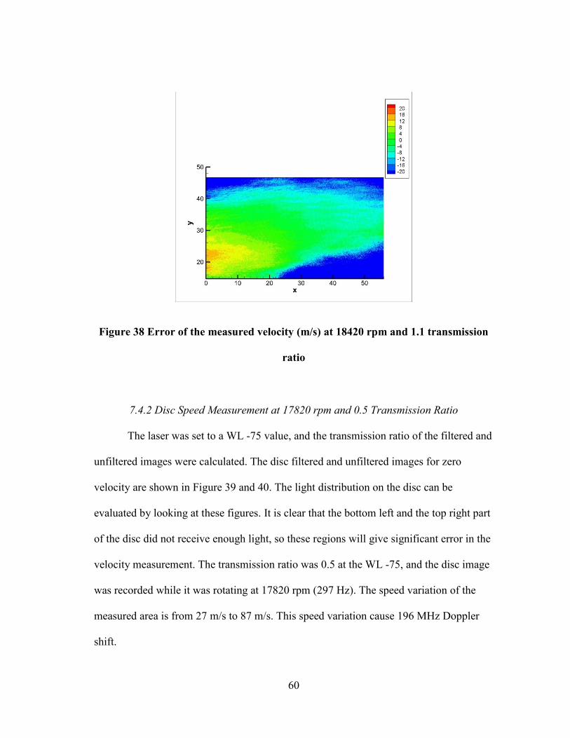
60


ratio


The laser was set to a WL -75 value, and the transmission ratio of the filtered and

unfiltered images were calculated. The disc filtered and unfiltered images for zero

velocity are shown in Figure 39 and 40. The light distribution on the disc can be

evaluated by looking at these figures. It is clear that the bottom left and the top right part

of the disc did not receive enough light, so these regions will give significant error in the

velocity measurement. The transmission ratio was 0.5 at the WL -75, and the disc image

was recorded while it was rotating at 17820 rpm (297 Hz). The speed variation of the

measured area is from 27 m/s to 87 m/s. This speed variation cause 196 MHz Doppler

shift.

61

The light variations on the disc can be seen in Figure 39 and 40, the images show

that the bottom right and the top part of the disc did not get enough light, so a significant

error is expected in these areas. The filtered and unfiltered lumens value of the disc can

be seen in Figure 41 and 42.

Figure 39 Filtered image of the disc at 0 rpm and 0.5 transmission ratio

62

Figure 40 Unfiltered image of the disc at 0 rpm and 0.5 transmission ratio


ratio

63

Figure 42 Lumen value of the unfiltered Image at 17820 rpm and 0.5 transmission

ratio

Figure 41 and 42 show that the bottom right and the top left part of the disc did

not get enough light because the lumen value goes to almost 0 at these points.

The transmission ratio of the ALF cell is 0.5 when the rotating disc was recorded,

and the frequency of the laser was known at this transmission ratio value and the

frequency shift of the disc can be calculated by using the frequency shift vs transmission

ratio graph. The transmission ratio changed by disc surface speed is shown in Figure 43.

64


The transmission ratio was converted to frequency using curve fit equations that

are shown in section 7.2. These equations calculate the frequency shift at each point by

using the transmission ratio. The calculated frequency distribution is shown in Figure 44.

65


The frequency of the laser is known when transmission ratio is 0.5 by the ALF

cell calibration graph. The frequency shift was calculated by subtracting the frequency of

the laser when the transmission ratio is 0.5 from the frequency distribution that is shown

in Figure 44. The frequency shift on the rotating disc calculated is shown in Figure 45.

66


(GHz)

The velocity of the rotating disc is calculated by using the frequency shift at each

point, and is shown in Figure 46. The speed of the disc is changing from 27 m/s to 87

m/s because the disc radius that was seen by cameras was from 14.7 mm to 46.7 mm.

There is significant error at the bottom right and the top left part because these parts did

not get enough laser light as mentioned for the previous measurement. The velocity error

of the disc is shown in Figure 47. The error is more than -20 m/s at the area that was not

received enough laser light. However, the error is relatively low at the area that was

received enough light for the measurement. Figure 47 shows the error, and the velocity

67

error is about ±2.5 m/s at the center of the disc because this region received enough

light.


68


ratio


The measurement was taken when the transmission ratio was 0.5 at the WL -75.

The speed of the disc was 10020 rpm (167 Hz), and the speed variations of the measured

area is from 15 m/s to 49 m/s since the radius of the observed area is from 14.7 mm to

46.7 mm. The Doppler shift of the disc is 110 MHz for this speed range.

The filtered and unfiltered images of rotating disc are shown in Figure 48 and 49,

and lumen value of the disc can be seen in Figure 48 and Figure 49. The bottom right

and the top left part of the disc did not get enough light, and that is shown in Figure 48

and 49 because the lumen value is almost 0 at these regions. The velocity result has a

significant error at these points because of that reason. The filtered and unfiltered images

lumens ratio figures show that clearly.

69


ratio


ratio

70

The transmission ratio difference is shown in Figure 50, the transmission ratio is

changing by velocity, and the ratio range is from 0.5 to 0.225. When the disc speed was

17820 rpm, the ratio range is from 0.5 to 0.075. The ratio is lower at high speed regions.

When Figure 43 and Figure 50 are compared that can be seen clearly.


The transmission ratio was converted to the frequency using the curve fit

equations that were shown in section 7.2 for 0.5 transmission ratio This equation

calculates the frequency at each point by using the transmission ratio. The calculated

frequency distribution is shown in Figure 51.

71


The frequency of the laser is known when the transmission ratio is 0.5 from the

ALF cell calibration graph. The frequency shift is calculated by subtracting the

frequency of the laser when the transmission ratio is 0.5 from the frequency distribution

that is shown in Figure 51. The frequency shift on the rotating disc is shown in Figure

52.

72


(GHz)

The velocity of the rotating disc is calculated using frequency shift at each point.

The speed of the disc is shown in Figure 53.

The error of the measured and actual velocity is shown in Figure 54. The error is

more than -20 m/s at the bottom left and the top right part because these regions did not

get enough light as mentioned before. The error is between -5 m/s and 2.5 m/s at the

center of the disc, but the error increased at the left part of the image and it is about 6.25

m/s.

73



ratio

74


The 18000 rpm (300 Hz) rotating disc images were recorded when the

transmission ratio is about 0.08. The filtered and unfiltered lumens ratios are shown in

Figure 55 and 56. The filtered lumen value is very low on the entire image because of

the low transmission ratio. Therefore, significant error is expected for this measurement

because the low lumen ratios cause uncertainty for the transmission ratio. The speed

range on the images is from 28 m/s to 87 m/s, which result is a 194 MHz frequency shift.

The transmission ratio is almost constant when it reaches the 0.08, and 194 MHz

frequency shift result in almost constant transmission ratio change, and that can be seen

in Figure 57. The velocity measurement was expected to be poor for this transmission

ratio measurement.

The 18000 rpm rotating disc surface speed was measured when the transmission

ratio was 0.08. When the transmission ratio is 0.08, the frequency shift is 1.8 GHz. The

18000 rpm surface speed causes a 194 MHz Doppler shift, so the expected frequency

shift of the laser is from 1.8 GHz to 1.94 GHz. When Figure 13is analyzed, the

transmission ratio change is almost constant between these frequency shift ranges. The

transmission ratio and the frequency shift relationship is key part of the DGV system to

measure velocity, so the transmission ratio should not be constant between measured

frequency shift ranges. Because of this reason, the velocity measurement of the surface

speed has significant error as expected.

75

Figure 55 Unfiltered image lumen ratio at 18000 rpm and 0.08 transmission ratio

Figure 56 Filtered image lumen ratio at 18000 rpm and 0.08 transmission ratio

76

The transmission ratio of the rotating disc image is shown in Figure 57. The

transmission ratio change is relatively small when it is compared with other

measurements, so the frequency shift calculation by using the transmission ratio has a

large error. The frequency change and frequency shift of the disc can be seen in Figure

58 and 59.


77

Figure 58 Frequency change on the disc at 18000 rpm and 0.08 transmission ratio

Figure 59 Frequency shift of the disc at 18000 rpm and 0.08 transmission ratio

The speed of the disc was calculated using the frequency shift of the disc that is

shown in the Figure 59. The speed result has a significant error as expected because the

78

frequency shift distribution on the disc much smaller it should be, so the speed result has

a significant error. The speed of the disc is shown in Figure 60.

Figure 60 Speed of the disc at 18000 rpm and 0.08 transmission ratio

79

8. CONCLUSION AND RECOMMENDATIONS

The primary objective of measuring velocity using a DGV system has been

achieved. The system is capable of measuring surface speed of a rotating disc.

8.1 Conclusion

A new DGV system was developed by upgrading to 12 bit CCD cameras, the

telecentric lens, the sealed iodine cell and a new laser.

The laser has an option to be controlled by a computer, and its wavelength can be

adjusted by using the WL code. Therefore, the frequency shift of the laser was calculated

by using the WL change because the WL and wavelength relation is known. Therefore,

the spectrum analyzer is not required part to obtain how the frequency of the laser shifts

by using the WL code.

The cameras that were used in Gaharan’s research were 8 bit (255 gray levels),

and its active imaging area is 240 horizontal by 512 vertical pixels. The cameras were

replaced in this study with 12 bit CCD cameras used to record the filtered and unfiltered

images. The CCD camera’s active imaging area is 1024x1024 pixel and gray levels are

4095. Also, the cameras’ intensity and spatial calibration are completed, so the system

can measure velocity of the area accurately. A Matlab code was created to perform

intensity calibration of 1048576 points for the filtered and unfiltered cameras. The

80

intensity calibration values and lumen conversion equations were calculated and saved

for each pixel locations.

The sealed iodine absorption line filter is a key part of the DGV system. The

calibration of the ALF cell allows the user to calculate frequency shift by using the

transmission ratio on each pixel. Therefore, a LabView code was created to calibrate the

ALF cell automatically. The code changes laser wavelength in a known range and power

meters measure the transmission ratio of the ALF cell for each known laser wavelength.

The relationship between the transmission ratio and the frequency shift of the laser is

calculated using this calibration process. Also, the power meters are used to observe any

drift on the laser frequency during data acquisition.

A 99.5 mm diameter rotating disc was used to produce a known velocity field to

evaluate the DGV system after all calibrations were completed. The surface speed of the

rotating disc was measured with three different transmission ratios. The transmission

ratios were 1.1, 0.5 and 0.08, and the rotational speed of the disc was about 18000 rpm.

The transmission ratio and frequency shift range was shown in the Figure 13 for all

transmission ratios.

The measured velocity had -8 to +12 m/s error when the transmission ratio was

1.1 at the regions that received sufficient illumination. The error of the surface speed

was ±5 m/s when the transmission ratio was 0.5 over the region that received enough

light. However, the error was significantly high at the bottom right and the left top part

because these regions did not receive enough light for these two measurements. There

was a significant error when the surface speed was measured at the 0.08 transmission

81

ratio. Since the transmission ratio change is constant between 1.8 GHz and 1.94 GHz at

18000 rpm when the transmission ratio is 0.08.

8.2 Recommendations

Many improvements can be applied to the DGV system apparatus which will

increase the accuracy of the system.

First, the CCD camera is an expensive apparatus of the DGV system, so the

camera number can be reduced for one dimensional measurement. Two CCD cameras

were used in our system for one dimensional measurement, but one camera can be used

with optical arrangement for one dimensional measurement. This system is achieved by

placing a mirror in front of the single CCD camera, and two images can be recorded side

by side. Even though using one camera would decrease the measured area, one camera

would reduce the cost of the DGV system. Also, two cameras would be enough to

measure two dimensional velocity measurement. Smith et al [8] implemented this

method.

Second, if the computer processor speed can be increased, calibration and data

reduction process times will decrease. The ALF cell calibration code can be modified,

and automatic image recording code can be added to the software. The modification was

used with the computer, but the modification slowed down the speed of the computer.

Also, the laser light did not cover the entire region that was seen by the cameras.

The new lens can be used to increase laser beam diameter to cover the region that is seen

by the cameras. There was a significant error in the regions that did not receive enough

light.

82

Many obstacles can be eliminated in the development and data acquisition of the

DGV system by following these recommendations.

83

REFERENCES

[1] Yeh, Y., and H. Z. Cummins, 1964, “Localized Fluid Flow Measurements with a

He-Ne Laser Spectrometer,” Applied Physics Letters, 4 (10), pp. 176-178.

[2] Komine, H., 1990, “System for Measuring Velocity Field of Fluid Flow Utilizing a

Laser-Doppler Spectral Image Converter,” United States Patent No. 4,919,536,

Northrop Corp., Hawthorne, CA.

[3] Meyers, J. F. and Komine, H., 1991, “Doppler Global Velocimetry A New Way to

Look at Velocity,” Proceedings of the ASME 4th International Conference on Laser

Anemometry, Cleveland, OH.

[4] Meyers, J. F., Lee, J. W. and Cavone, A. A., 1991, “Signal Processing Schemes for

Doppler Global Velocimetry,” IEEE – 14th International Congress on

Instrumentation in Aerospace Simulation Facilities, Rockville, MD.

[5] Meyers, J. F., 1992, “Doppler Global Velocimetry-The Next Generation?” AIAA

Paper 92-3897.

[6] Meyers, J. F., 1994, “Development of Doppler Global Velocimetry for Wind

Tunnel Testing,” AIAA Paper 94-2582.

[7] Ford, H. D. and R. P. Tatam, 1995, “Imaging System Considerations in Doppler

Global Velocimetry,” Proceedings of SPIE 2546, Optical Techniques in Fluid,

Thermal, and Combustion Flow, 2546 pp. 454- 464.

84

[8] Smith, M. W., Northam, G. B. and Drummond, J. P., 1996, “Application of

Absorption Filter Planar Doppler Velocimetry to Sonic and Supersonic Jets,” AIAA

Journal, 34 (3), pp.434-441.

[9] Smith, M. W., 1998, “The Reduction of Laser Speckle Noise in Planar Doppler

Velocimetry Systems,” AIAA Paper 98-2607.

[10] McKenzie, R. L., 1996, “Measurement Capabilities of Planar Doppler Velocimetry

Using Pulsed Lasers,” Applied Optics, 35 (6), pp. 948-964.

[11] McKenzie, R. L., 1997, “Planar Doppler Velocimetry Performance in Low-Speed

Flows,” AIAA Paper 97-0498.

[12] Morrison, G. L., Gaharan C. A., and DeOtte Jr, R. E, 1995, “Doppler Global

Velocimetry: Problems and Pitfalls,” Flow Measurement and Instrumentation, 6

(2), pp. 83-91.

[13] Roehle, I., 1996, “Three-dimensional Doppler Global Velocimetry in the Flow of a

Fuel Spray Nozzle and in the Wake Region of a Car,” Flow Measurement and

Instrumentation 7 (3-4), pp. 287-294.

[14] Muller, H., Lemacher, T., Pape, N., Strunck, V., and Dophenide, D., 2008, “3D-

DGV for Flow Field Investigation in Pipes,” Physikalisch-Technische

Bundesanstalt, Braunschweig, Germany.

[15] Nobes, D. S., Ford, H. D., and Tatam, R. P., 2004, “Instantaneous, Three-

Component Planar Doppler Velocimetry Using Imaging Fibre Bundles,”

Experiments in Fluids 36 (1), pp. 3-10.

85

[16] Willert, C., Stockhausen, G., Klinner, J., Lempereur, C., Barricau, P., Loiret, P., and

Raynal, J. C., 2007, “Performance and Accuracy Investigations of Two Doppler

Global Velocimetry Systems Applied in Parallel,” Measurement Science and

Technology, 18 (8), pp. 2504-2512.

[17] Arnette, S. A., Elliott, G. S., and Mosedale, A. D. and Carter, C. D., 2000, “Two-

Color Planar Doppler Velocimetry,” AIAA Journal 38 (11), pp. 2001-2006.

[18] Willert, C., Hassa, C., Stockhausen, G., Jarius, M., Voges, M., and Klinner, J.,

2006, “Combined PIV and DGV Applied to a Pressurized Gas Turbine Combustion

Facility,” Measurement Science and Technology, 17 (7), pp. 1670-1679.

[19] Chan, V. S. S., Heyes, A. L., Robinson, D. I., and Turner, J. T., 1995, “Iodine

Absorption Filters for Doppler Global Velocimetry,” Measurement Science and

Technology, 6 (6), pp. 784-794.

[20] Miles, R. B., Lempert, W. R., and Forkey, J., 1991, “Instantaneous Velocity Fields

and Background Suppression by Filtered Rayleigh Scattering,” AIAA Paper 91-

0357.

[21] Naylor S., and Kuhlman J., 1997, “Accuracy Studies of a Two-Component Doppler

Global Velocimeter (DGV),” AIAA Paper 97-0508.

[22] Gaharan, C. A., 1996, “The Development of a Doppler Global Velocimeter and Its

Image Processing Schemes for Whole-Field Measurements of Velocity,” PhD

Dissertation, Texas A&M University, College Station, Texas.

86

[23] Nelson, B., 2008, “The Development of a Frequency Control System of a Seeded

Laser for DGV Application”, MSc Thesis, Texas A&M University, College Station,

Texas.

the development of an accuracy of a doppler …

Documents