the development of a monolithic shape memory alloy …
TRANSCRIPT
THE DEVELOPMENT OF A
MONOLITHIC
SHAPE MEMORY ALLOY ACTUATOR
by
Leslie Marilyn Toews
A thesis
presented to the University of Waterloo
in fulfillment of the
thesis requirement for the degree of
Master of Applied Science
in
Electrical and Computer Engineering
Waterloo, Ontario, Canada, 2004
c©Leslie Marilyn Toews 2004

I hereby declare that I am the sole author of this thesis. This is a true copy of the
thesis, including any required final revisions, as accepted by my examiners.
I understand that my thesis may be made electronically available to the public.
ii
Abstract
Shape memory alloys (SMAs) provide exciting opportunities for miniature ac-
tuation systems. As SMA actuators are scaled down in size, cooling increases and
bandwidth improves. However, the inclusion of a bias element with which to cycle
the SMA actuator becomes difficult at very small scales.
One technique used to avoid the necessity of having to include a separate bias
element is the use of local annealing to fabricate a monolithic device out of nickel
titanium (NiTi). The actuator geometry is machined out of a single piece of non-
annealed NiTi. After locally annealing a portion of the complete device, that section
exhibits the shape memory effect while the remainder acts as structural support
and provides the bias force required for cycling.
This work proposes one such locally-annealed monolithic SMA actuator for fu-
ture incorporation in a device that navigates the digestive tract. After detailing
the derivation of lumped electro-mechanical models for the actuator, a descrip-
tion of the prototyping procedure, including fabrication and local annealing of the
actuator, is provided. This thesis presents the experimental prototype actuator
behaviour and compares it with simulations generated using the developed models.
iii

Acknowledgments
One of the wonderful things about life is the amazing people that surround us.
Many from university, industry, and the surrounding community continually share
their knowledge and resources with me. I would like to take this opportunity to
thank some who have invested in this research.
I would like to thank my supervisor Robert B. Gorbet for giving me the opportu-
nity to work on this project and for the guidance he provided throughout. Thank
you to Nitinol Devices & Components for providing the Nitinol strips. Thank
you to Laurie Cowell for providing clay to create the clay fixture. Thank you to
Baumeier Waterjet Technology for producing the actuators. Thank you to John
Boldt, Richard Forgett, Fred Bakker, Robert Wagner, and Robert Kaptein for pro-
ducing the aluminium fixture or for just being helpful. Andrew Smith, thank you
for your approachability and for giving me Nichrome strips. Thank you to Richard
Gordon for flattening the Nichrome strips. Thank you to Steven Corbin for suggest-
ing electroplating and soldering. Alan Hodgson, thank you for teaching me how
to spot weld and for soldering the Nichrome strips. Thank you to Denise Carla
Corsil-Gosselink for helping me make an electrolyte. Thank you to Norval Wilhelm
for teaching me how to electroplate. Brian Keats, thank you for giving me access
to your temperature program and for helping me with various details. Thank you
to Marlene Toews Janzen for editing my thesis. Thank you to David W.L. Wang
and Glenn R. Heppler for reviewing my thesis. Thank you to all the friends who
have helped make my Master’s a wonderful experience.
I am also extremely grateful for the love of my family, Victor, Lorraine, and
Mark Toews, and for the continued prayers of my Grandma. Their support always
encourages and sustains me.
iv

Dedication
“Miracles happen on roads less travelled. As you journey through life, enjoy the
detours.”
- Anonymous
“Twenty years from now, you will be more disappointed by the things you didn’t
do than by the ones you did. So throw off the bowlines. Sail away from the safe
harbour. Catch the trade winds in your sails. Explore. Dream. Discover.”
- Anonymous
v

Contents
1 Introduction 1
1.1 Motivation . . . . . . . . . . . . . . . . . . . . . . . . . . . . . . . . 1
1.2 Goals and Scope . . . . . . . . . . . . . . . . . . . . . . . . . . . . 3
1.3 Overview . . . . . . . . . . . . . . . . . . . . . . . . . . . . . . . . . 4
2 Background 5
2.1 Digestive Tract . . . . . . . . . . . . . . . . . . . . . . . . . . . . . 5
2.1.1 Dimensional Constraints of the Digestive Tract . . . . . . . 7
2.1.2 Other Physiological Considerations of the Digestive Tract . . 7
2.1.3 Digestive Medical Technology . . . . . . . . . . . . . . . . . 9
2.1.4 Digestive Tract Summary . . . . . . . . . . . . . . . . . . . 13
2.2 Meso-Scale Actuation . . . . . . . . . . . . . . . . . . . . . . . . . . 14
2.3 Shape Memory Alloys . . . . . . . . . . . . . . . . . . . . . . . . . 19
2.3.1 Shape Memory Effect . . . . . . . . . . . . . . . . . . . . . . 20
2.3.2 Shape Memory Alloy Microscopic Properties . . . . . . . . . 21
vi
2.3.3 Phase Transformation . . . . . . . . . . . . . . . . . . . . . 23
2.3.4 Shape Memory Alloy Macroscopic Behaviour . . . . . . . . . 28
2.3.5 Shape Memory Alloy Actuator Design . . . . . . . . . . . . 34
2.3.6 Monolithic Shape Memory Alloy Actuator . . . . . . . . . . 38
2.3.7 Shape Memory Alloy Applications . . . . . . . . . . . . . . . 40
2.3.8 Shape Memory Alloy Summary . . . . . . . . . . . . . . . . 42
3 Analytical Model Development 44
3.1 Proposed Geometry . . . . . . . . . . . . . . . . . . . . . . . . . . . 44
3.2 System Model . . . . . . . . . . . . . . . . . . . . . . . . . . . . . . 47
3.3 Mechanical Equivalent Lumped Model . . . . . . . . . . . . . . . . 51
3.4 Equivalent Stiffness of Annealed Beam . . . . . . . . . . . . . . . . 53
3.4.1 Young’s Modulus to Stiffness Model . . . . . . . . . . . . . . 54
3.4.2 Linear Temperature to Young’s Modulus Model . . . . . . . 55
3.4.3 Stress and Strain Model . . . . . . . . . . . . . . . . . . . . 56
3.4.4 Phase Model . . . . . . . . . . . . . . . . . . . . . . . . . . 63
3.4.5 Heating Model . . . . . . . . . . . . . . . . . . . . . . . . . 70
3.5 Equivalent Mass of Annealed Beam . . . . . . . . . . . . . . . . . . 71
3.6 Equivalent Stiffness of Non-Annealed Portal . . . . . . . . . . . . . 73
3.7 Equivalent Mass of Non-Annealed Portal . . . . . . . . . . . . . . . 79
3.8 Equivalent System Summary . . . . . . . . . . . . . . . . . . . . . . 82
vii
4 Dimension Selection and Parameters 84
5 Analytical Simulations 93
5.1 Linear Young’s Modulus System Model . . . . . . . . . . . . . . . . 93
5.2 Non-Linear Young’s Modulus System Model . . . . . . . . . . . . . 94
5.3 Simulation Results . . . . . . . . . . . . . . . . . . . . . . . . . . . 96
6 Monolithic Prototype Fabrication 104
6.1 Machining of Actuator . . . . . . . . . . . . . . . . . . . . . . . . . 106
6.2 Fixture Design and Heating Method . . . . . . . . . . . . . . . . . 108
6.2.1 Fixture . . . . . . . . . . . . . . . . . . . . . . . . . . . . . . 110
6.2.2 Heating Element . . . . . . . . . . . . . . . . . . . . . . . . 117
6.2.3 Mating Piece . . . . . . . . . . . . . . . . . . . . . . . . . . 131
6.2.4 Electrical Insulator . . . . . . . . . . . . . . . . . . . . . . . 133
6.2.5 Fixture Design and Heating Method Summary . . . . . . . . 134
6.3 Middle Beam Shape-Setting Process . . . . . . . . . . . . . . . . . . 134
6.3.1 Effect of Fixture . . . . . . . . . . . . . . . . . . . . . . . . 135
6.3.2 Effect of Forced Convection . . . . . . . . . . . . . . . . . . 138
6.3.3 Effect of Mating Piece . . . . . . . . . . . . . . . . . . . . . 142
6.3.4 Annealing of the Actuator . . . . . . . . . . . . . . . . . . . 142
6.3.5 Monolithic Prototype Summary . . . . . . . . . . . . . . . . 145
viii
7 Prototype Testing 146
7.1 Nature of Actuator . . . . . . . . . . . . . . . . . . . . . . . . . . . 149
7.1.1 Deformation Test . . . . . . . . . . . . . . . . . . . . . . . . 149
7.1.2 Continual Cycling Test . . . . . . . . . . . . . . . . . . . . . 153
7.1.3 Nature of Actuator Summary . . . . . . . . . . . . . . . . . 156
7.2 Nature of Actuator’s Middle Beam . . . . . . . . . . . . . . . . . . 156
7.3 Nature of Actuator’s Portal . . . . . . . . . . . . . . . . . . . . . . 158
7.4 Prototype Testing using Current . . . . . . . . . . . . . . . . . . . . 159
7.5 Microstructure . . . . . . . . . . . . . . . . . . . . . . . . . . . . . 162
7.6 Prototype Testing Summary . . . . . . . . . . . . . . . . . . . . . . 163
8 Discussion 165
8.1 Result Comparison . . . . . . . . . . . . . . . . . . . . . . . . . . . 165
8.2 Portal Buckling . . . . . . . . . . . . . . . . . . . . . . . . . . . . . 166
8.3 Differing Factors . . . . . . . . . . . . . . . . . . . . . . . . . . . . 167
8.3.1 Dimensional Differences . . . . . . . . . . . . . . . . . . . . 167
8.3.2 Property Values . . . . . . . . . . . . . . . . . . . . . . . . . 168
8.4 Obtaining Measurements . . . . . . . . . . . . . . . . . . . . . . . . 168
8.5 Discussion Summary . . . . . . . . . . . . . . . . . . . . . . . . . . 169
9 Conclusions 170
ix
10 Future Work 173
10.1 Assumption Improvements . . . . . . . . . . . . . . . . . . . . . . . 173
10.2 Dimension Selection . . . . . . . . . . . . . . . . . . . . . . . . . . 174
10.3 Fabrication Techniques . . . . . . . . . . . . . . . . . . . . . . . . . 175
10.4 Cyclic Behaviour . . . . . . . . . . . . . . . . . . . . . . . . . . . . 176
10.5 Other Milestones . . . . . . . . . . . . . . . . . . . . . . . . . . . . 176
10.6 Future Work Summary . . . . . . . . . . . . . . . . . . . . . . . . . 177
Bibliography 178
List of Nomenclature 186
List of Acronyms and Chemical Formulas 192
x

List of Figures
1.1 Artist’s conception of preliminary robot design . . . . . . . . . . . . 2
2.1 Digestive tract . . . . . . . . . . . . . . . . . . . . . . . . . . . . . . 6
2.2 M2A r© capsule . . . . . . . . . . . . . . . . . . . . . . . . . . . . . 12
2.3 Inchworm-type robot for colon inspection . . . . . . . . . . . . . . . 14
2.4 Micro-fabricated car . . . . . . . . . . . . . . . . . . . . . . . . . . 15
2.5 Piezoelectric-based locomotion technique . . . . . . . . . . . . . . . 16
2.6 Meso-scale actuator with interlocking micro-ridges . . . . . . . . . . 17
2.7 Dual-diaphragm pump . . . . . . . . . . . . . . . . . . . . . . . . . 18
2.8 Austenite . . . . . . . . . . . . . . . . . . . . . . . . . . . . . . . . 21
2.9 Twinned martensite . . . . . . . . . . . . . . . . . . . . . . . . . . . 22
2.10 Detwinned martensite . . . . . . . . . . . . . . . . . . . . . . . . . 22
2.11 Transformation temperatures . . . . . . . . . . . . . . . . . . . . . 25
2.12 Temperature-to-phase hysteresis with major and minor loops . . . . 27
2.13 SMA stress-strain curves . . . . . . . . . . . . . . . . . . . . . . . . 29
2.14 Shape memory process . . . . . . . . . . . . . . . . . . . . . . . . . 31
xi

2.15 Loaded SMA macroscopic behaviour . . . . . . . . . . . . . . . . . 33
2.16 SMA spring under constant load . . . . . . . . . . . . . . . . . . . . 35
2.17 Spring-biased SMA actuator . . . . . . . . . . . . . . . . . . . . . . 36
2.18 Spring-biased SMA actuator with external load . . . . . . . . . . . 37
2.19 Monolithic translation stage . . . . . . . . . . . . . . . . . . . . . . 39
2.20 SMA gripper design . . . . . . . . . . . . . . . . . . . . . . . . . . . 40
2.21 Active catheter . . . . . . . . . . . . . . . . . . . . . . . . . . . . . 41
3.1 Proposed actuator design . . . . . . . . . . . . . . . . . . . . . . . . 45
3.2 Tip displacement . . . . . . . . . . . . . . . . . . . . . . . . . . . . 46
3.3 Mass-spring-damper system . . . . . . . . . . . . . . . . . . . . . . 48
3.4 Actuator and lumped model . . . . . . . . . . . . . . . . . . . . . . 49
3.5 Block diagram for the linear Young’s modulus system model . . . . 50
3.6 Block diagram for the non-linear Young’s modulus system model . . 51
3.7 Coordinate system showing tip displacement . . . . . . . . . . . . . 52
3.8 Mechanical equivalent lumped model . . . . . . . . . . . . . . . . . 52
3.9 Free-body diagram of lumped model . . . . . . . . . . . . . . . . . 53
3.10 Curved cantilever . . . . . . . . . . . . . . . . . . . . . . . . . . . . 55
3.11 Temperature-to-phase hysteresis with major and minor loops . . . . 57
3.12 Variable sublayer model . . . . . . . . . . . . . . . . . . . . . . . . 58
3.13 SMA stress-strain curves . . . . . . . . . . . . . . . . . . . . . . . . 60
3.14 Cantilever with end-point load . . . . . . . . . . . . . . . . . . . . . 62
xii

3.15 Block diagram of stress and strain model . . . . . . . . . . . . . . . 63
3.16 RmaC(t) and Rma
H(t) at switching times . . . . . . . . . . . . . . . 67
3.17 Element of beam in bending . . . . . . . . . . . . . . . . . . . . . . 72
3.18 Non-annealed portal . . . . . . . . . . . . . . . . . . . . . . . . . . 74
3.19 Portal free-body diagram . . . . . . . . . . . . . . . . . . . . . . . . 75
3.20 Girder loading . . . . . . . . . . . . . . . . . . . . . . . . . . . . . . 76
3.21 Twist of cantilever due to moment . . . . . . . . . . . . . . . . . . 77
3.22 Simply-supported beam with mid-beam load . . . . . . . . . . . . . 78
4.1 Tension test using as-rolled NiTi sample . . . . . . . . . . . . . . . 87
4.2 Tension test using martensite NiTi sample . . . . . . . . . . . . . . 88
4.3 Monolithic actuator dimensions . . . . . . . . . . . . . . . . . . . . 89
4.4 Circle segment . . . . . . . . . . . . . . . . . . . . . . . . . . . . . . 91
5.1 Linear Young’s modulus system model . . . . . . . . . . . . . . . . 94
5.2 Non-linear Young’s modulus system model . . . . . . . . . . . . . . 94
5.3 Computing Eb for non-linear model . . . . . . . . . . . . . . . . . . 95
5.4 Temperature of annealed beam and input current . . . . . . . . . . 97
5.5 Martensite phase fraction of annealed beam and input current for
non-linear model . . . . . . . . . . . . . . . . . . . . . . . . . . . . 98
5.6 Young’s modulus of annealed beam and input current . . . . . . . . 99
5.7 Tip deflection of annealed beam and input current . . . . . . . . . . 100
5.8 Martensite phase fraction and temperature of annealed beam . . . . 101
xiii

6.1 Composite prototype and clay fixture . . . . . . . . . . . . . . . . . 106
6.2 Conventionally machined monolithic actuator . . . . . . . . . . . . 107
6.3 Waterjet-manufactured monolithic actuators . . . . . . . . . . . . . 109
6.4 Side view of fixture prototyping apparatus . . . . . . . . . . . . . . 110
6.5 Fixture . . . . . . . . . . . . . . . . . . . . . . . . . . . . . . . . . . 111
6.6 Top die . . . . . . . . . . . . . . . . . . . . . . . . . . . . . . . . . 112
6.7 Bottom die . . . . . . . . . . . . . . . . . . . . . . . . . . . . . . . 113
6.8 Fixture simulation at one minute . . . . . . . . . . . . . . . . . . . 118
6.9 Fixture simulation at two minutes . . . . . . . . . . . . . . . . . . . 119
6.10 Electroplating apparatus . . . . . . . . . . . . . . . . . . . . . . . . 121
6.11 Electroplated strip of Nichrome . . . . . . . . . . . . . . . . . . . . 122
6.12 “Burned-looking” electroplated strip of Nichrome . . . . . . . . . . 123
6.13 Copper-brazed Nichrome . . . . . . . . . . . . . . . . . . . . . . . . 125
6.14 Temperature of a copper-brazed Nichrome strip . . . . . . . . . . . 126
6.15 Experimental set-up for current-to-temperature test . . . . . . . . . 128
6.16 Thermocouples and electrical leads on Nichrome strip . . . . . . . . 128
6.17 Temperature of a silver-tin end-soldered Nichrome strip . . . . . . . 129
6.18 Solder at ends of Nichrome strip . . . . . . . . . . . . . . . . . . . . 131
6.19 Ceramic mating piece . . . . . . . . . . . . . . . . . . . . . . . . . . 132
6.20 Voltage of Nichrome strip as a function of surroundings . . . . . . . 136
6.21 Temperature of Nichrome strip as a function of surroundings . . . . 137
xiv
6.22 Temperature of Nichrome strip in fixture with convection . . . . . . 139
6.23 Mid-point temperature of middle beam in fixture with convection . 140
6.24 End-point temperature of middle beam in fixture with convection . 141
6.25 Effect of mating piece at the middle beam mid-point . . . . . . . . 143
6.26 Effect of mating piece at the middle beam end-point . . . . . . . . . 144
7.1 Samples after application of upward force . . . . . . . . . . . . . . . 148
7.2 Samples after application of downward force . . . . . . . . . . . . . 148
7.3 Deformation test . . . . . . . . . . . . . . . . . . . . . . . . . . . . 150
7.4 Continual cycling test . . . . . . . . . . . . . . . . . . . . . . . . . . 154
7.5 Prototype testing using current . . . . . . . . . . . . . . . . . . . . 160
xv

List of Tables
3.1 Proportionality constant for twist of beams . . . . . . . . . . . . . . 78
4.1 Actuator dimensions . . . . . . . . . . . . . . . . . . . . . . . . . . 85
4.2 Simulation parameters . . . . . . . . . . . . . . . . . . . . . . . . . 86
4.3 Model parameter calculations . . . . . . . . . . . . . . . . . . . . . 90
6.1 Composition of a copper-sulfate bath . . . . . . . . . . . . . . . . . 120
7.1 Deformation test: SA direction of anneal . . . . . . . . . . . . . . . 151
7.2 Deformation test: SA direction opposite anneal . . . . . . . . . . . 151
7.3 Deformation test: SB direction of anneal . . . . . . . . . . . . . . . 152
7.4 Deformation test: SB direction opposite anneal . . . . . . . . . . . 152
7.5 Summary of averaged deformation tests of samples . . . . . . . . . 153
7.6 Continual cycling tests of samples . . . . . . . . . . . . . . . . . . . 155
7.7 Summary of continual cycling tests of samples . . . . . . . . . . . . 155
7.8 Deformation test: SB middle beam . . . . . . . . . . . . . . . . . . 157
7.9 Continual cycling test: SB middle beam . . . . . . . . . . . . . . . 158
xvi

7.10 First deformation test of SC . . . . . . . . . . . . . . . . . . . . . . 161
7.11 Second deformation test of SC . . . . . . . . . . . . . . . . . . . . . 161
7.12 Third deformation test of SC . . . . . . . . . . . . . . . . . . . . . . 161
xvii

Chapter 1
Introduction
1.1 Motivation
According to the American College of Gastroenterology, each year more than ninety-
five million people in the United States have a digestive problem and over ten million
are hospitalised for related treatments [1]. The types and severity of digestive
problems vary. The National Cancer Institute cites cancers of the colon as the fourth
most commonly diagnosed cancers and as the second cause of cancer deaths in the
United States [2]. Approximately two percent of the adult American population
suffers from Gastroesophageal Reflux Disease (GERD) while more than one million
Americans are estimated to suffer from Inflammatory Bowel Disease (IBD) [3], [4].
Early diagnosis and detection are fundamental in the treatment of these prob-
lems. Conventional endoscopic procedures are some of the preferred diagnostic and
therapeutic techniques. Colon cancers, GERD, and IBD can be diagnosed with
endoscopes. However, due to difficulty in controlling and manipulating the scopes,
these techniques do not permit investigation of most of the six metres of the small
1
intestine [5]. Also, the pain and discomfort of endoscopy make this procedure un-
popular.
As a result, an Israeli physician, Dr. Gavriel Iddan, developed a swallowable
capsule that contains a tiny video camera, lights, transmitter, and batteries [6].
This capsule allows for the investigation of the small intestine. However, it does
not function in the colon or stomach [2]. Also, it has a limited field of view and
is not physician controlled. Therefore, this technology is unable to diagnose many
digestive ailments since some lesions may go undetected because of the random
camera orientation.
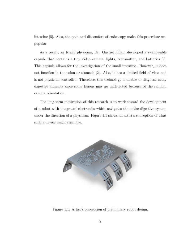
The long-term motivation of this research is to work toward the development
of a robot with integrated electronics which navigates the entire digestive system
under the direction of a physician. Figure 1.1 shows an artist’s conception of what
such a device might resemble.
Figure 1.1: Artist’s conception of preliminary robot design.
2

One challenge of this long-term objective is the design of the locomotion system
for the robot. The focus of the current work is the use of shape memory alloy
(SMA) in the development of a prototype actuator. SMAs fall into the category of
so-called “smart materials”. SMA actuators are smooth, silent, scalable, and have
very high power-to-mass ratios. These latter two properties make them ideal for
consideration for miniaturization.
1.2 Goals and Scope
The behaviour of an SMA actuator depends on material properties as well as ac-
tuator geometry. Once a specific geometry is proposed, the development of the
actuator requires achieving the following goals:
• to develop a lumped model for the proposed actuator,
• to simulate its behaviour,
• to prototype the design, and
• to compare the experimental prototype behaviour with the predicted model
behaviour.
In the course of this work, various assumptions have been made. These as-
sumptions are discussed in each chapter. Chapter 2 provides background in a
number of specific areas, but it is assumed that the reader has a basic knowledge
of the fundamentals of heat transfer and mechanics of materials [7], [8]. Physio-
logical considerations, such as environmental fragility and acidity, are important
to the long-term goals of this research. While these topics are briefly examined in
Chapter 2, they are not explicitly considered in the actuator design at this stage.
3
1.3 Overview
This work outlines the development of a monolithic SMA actuator. Following this
introductory chapter, a lumped model is developed and simulated. The results of
model simulations are compared to and discussed in light of experimental results
obtained from a prototype. Finally, conclusions and the direction of future work
are outlined. The specific organization of the thesis is outlined here.
Chapter 2 focuses on background information and others’ progress in related
research areas.
Chapter 3 details the development of a lumped model for the proposed actuator
geometry. The derivation of lumped model parameters and their relation to the
actual system is discussed.
In Chapter 4, dimensions for a centimetre-scale monolithic SMA actuator are
chosen, and the material properties are listed.
In Chapter 5, the results of analytical simulations using the model from Chapter 3
are provided.
A prototype is constructed to determine the model’s validity. Chapter 6 dis-
cusses the procedure used to fabricate the proof-of-concept prototype.
Chapter 7 discusses the success of the prototype fabrication process by observing
experimental prototype behaviour.
In Chapter 8, the results from analytical simulations and actual experiments
are compared.
Chapter 9 lists the conclusions while Chapter 10 discusses future work.
4

Chapter 2
Background
Since the long-term research goal is to create a miniature SMA robot for use in
the digestive tract, it is beneficial to discuss the intended operating environment,
small-scale actuation, and the proposed material.
2.1 Digestive Tract
The digestive tract, also known as the gastrointestinal (GI) tract and the alimentary
tract, is one of the major body systems. Its purposes include converting food from
the external environment into nutrients and eliminating solid wastes. Figure 2.1 is
a schematic of the digestive system.
A brief discussion of the digestive tract’s dimensional constraints and other
physiological constraints precedes an overview of digestive medical technology.
5
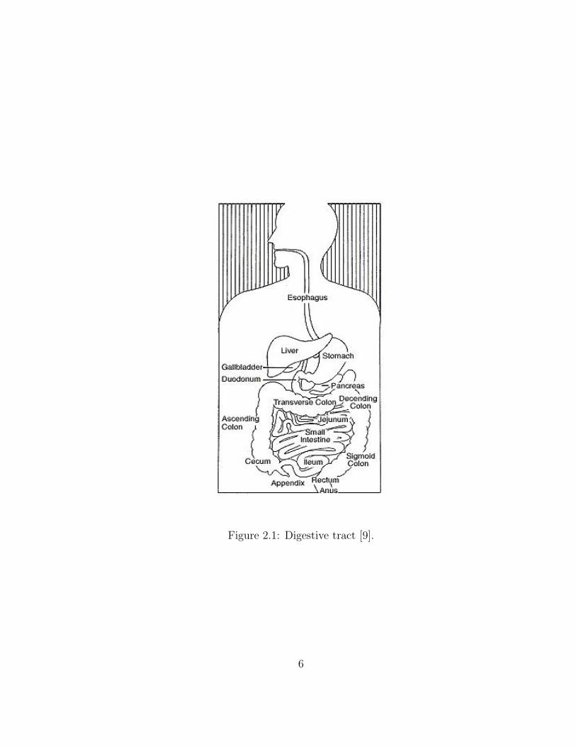
Figure 2.1: Digestive tract [9].
6
2.1.1 Dimensional Constraints of the Digestive Tract
The GI tract’s cavity is continuous with the environment since it is open at both
ends. Indigestible materials, such as cellulose from plant walls or a miniature
robot, pass from the mouth to the anus without crossing the epithelial lining of the
digestive tract.
Normally, when the esophagus is not in use, its upper and lower sphincters
contract so that food and stomach acid do not flow up from the stomach to the
mouth. When a person swallows, these sphincters relax [10]. This relaxation allows
the material to pass through the esophagus and enter the stomach.
After the swallowed material leaves the stomach, it proceeds through the small
and large intestines. The intestine’s smallest radius is between 20mm and 30mm,
and it is located at the boundary between the rectum and the sigmoid colon [11].
Any device navigating the colon must be able to pass through this region.
The narrowest part of the digestive tract is the pharynx at the esophagus junc-
tion with a diameter of approximately 15mm [12]. Hence, any robot used in the
digestive tract must have a diameter of less than 15mm.
2.1.2 Other Physiological Considerations of the Digestive
Tract
Other physiological factors require consideration. These include functional types of
movement, pressure, and media.
Knowing the movements in the digestive tract provides insight into the possible
interaction of the robot with its surroundings. There are two functional types of
movements in the digestive tract: propulsive and mixing movements. Propulsive
7
movements cause food to move forward along the tract at an appropriate rate for di-
gestion and absorption; mixing movements keep the intestinal contents thoroughly
mixed at all times [10]. Different sections of the tract use variations of these move-
ments. The maximum frequency of contractions in the small intestine is determined
by the frequency of the slow waves in the intestinal wall and occurs at a frequency
of about twelve per minute [10]. Peristaltic waves occur in any part of the small
intestine and move anal-ward at a velocity of 0.5 cms
to 2.0 cms
; the peristaltic waves
move much faster in the proximal intestine and much slower in the terminal intes-
tine [10]. After the food has mixed with stomach secretions, the resulting mixture
that passes down the gut is called chyme. The net movement of chyme along the
small intestine averages only 1 cmmin
.
Various pressures exist throughout the digestive tract. Between swallows, the
upper esophageal sphincter remains strongly contracted with a pressure as high
as 8 000Pa in the esophageal lumen [10]. This great pressure prevents air from
going into the esophagus during respiration. At the lower end of the esophagus, the
esophageal circular muscle functions as a lower esophageal sphincter. Usually, it
remains tonically constricted with an intra-luminal pressure of about 4 000Pa [10].
Intense peristaltic contractions used to empty the stomach often create pressures
between 4 903Pa to 6 865Pa. This is about six times as powerful as the usual mixing
type of peristaltic waves [10]. The completely relaxed stomach can store about 1.5 L
of food. The pressure in the stomach remains low until this limit is approached
[10]. Pressure fluctuations are also caused by breathing hard and coughing [10].
The medium surrounding the robot will affect the robot’s performance. The
type of digestive juice, amount, and acidity vary along the digestive tract. The
stomach’s contents are highly acidic [10]. The degree of fluidity of chyme depends
on the relative ratio of food to stomach secretions and on the degree of digestion
8
that has occurred. Whenever the pH of the chyme in the duodenum falls below 3.5
to 4, intestinal reflexes frequently block further release of acidic stomach contents
into the duodenum until the duodenal chyme can be neutralized by pancreatic and
other secretions [10]. Accordingly, it is important to develop a robot that will
be able to function in a worst-case scenario or at minimum be excreted without
damaging the tract.
2.1.3 Digestive Medical Technology
Various diseases and medical problems require a physician to investigate the diges-
tive tract using tools that demand a high degree of dexterity. Patients find many
of these procedures painful and uncomfortable. However, advances in technology
have led to more patient-friendly devices.
Conventional endoscopy is a procedure that uses a medical device, consisting of
a camera mounted on a flexible tube, to investigate the digestive tract trans-orally
or trans-anally. It is the standard for diagnosis and treatment of the upper 1.2m
and lower 1.8m of the digestive tract [5]. A gastroscopy is an endoscopic procedure
that uses a scope in the upper section, including the esophagus, stomach, and
duodenum. A colonoscopy is an endoscopic procedure that uses a scope in the lower
section, including the rectum and colon. Approximately 6.1m of small intestine is
inaccessible by scope.
Though endoscopes give medical professionals access to sections of the digestive
tract without surgery, there are weaknesses associated with this technology. Some
of these include difficulty in manoeuvring the scope, significant medical training
required for those using the scope, and patient discomfort. Also, in colonoscopies,
the gut’s peristaltic action impedes the use of a scope [13]. Despite these difficulties,
9
endoscopy is the preferred investigative procedure for upper gastrointestinal bleed-
ing because of its accuracy, low rate of complications, and potential for therapeutic
intervention [14]. However, there is a desire to improve the safety and reduce the
cost of endoscopy.
An alternative tool for endoscopy that seeks to improve safety and reduce cost is
the ultra-thin endoscope. Standard diagnostic gastroscopes are 9mm in diameter;
those used for therapeutic procedures in the upper tract are typically 11mm in di-
ameter. Ultra-thin endoscopes have an outer diameter between 5.3mm and 5.9mm
[14]. Such thin instruments can be inserted either trans-orally or trans-nasally
with reasonable ease. It is hypothesized that these scopes will lead to endoscopic
procedures that do not require sedation. Because a substantial proportion of en-
doscopic procedure-related complications are due to sedation, the performance of
endoscopy without sedation is a worthwhile goal that would improve patient safety.
Also, endoscopy without sedation would reduce costs substantially by eliminating
the need for sedatives, hemodynamic monitoring during the procedure, time in the
recovery room, some of the nursing staff, a day off from work by the patient, and
an escort to accompany the patient home from the procedure [14]. Unfortunately,
even ultra-thin endoscopes do not permit visualization of the entire digestive tract.
When gastrointestinal blood loss cannot be related to a specific cause after a
gastroscopy or a colonoscopy, an examination of the small intestine is performed
either with push enteroscopy, operative endoscopy, or sonde (passive) enteroscopy
[14]. Push enteroscopy uses a longer endoscopic instrument that is difficult to con-
trol and manipulate due to its length. In operative endoscopy, the surgeon advances
the endoscope manually through the surgically exposed intestine. Since this is a
surgical procedure, the recovery time is more significant. In sonde enteroscopy, the
tip of a small-caliber enteroscope, whose length varies between 270 cm and 400 cm,
10
moves passively along the small intestine. Though these traditional methods offer
some insight into the potential problem, they do not give the medical professional
easy access to the small intestine.
Special imaging studies, computerised tomography (CT) and magnetic reso-
nance imaging (MRI) scans, do not provide the detail necessary for small intestine
investigation. The small bowel series, which includes x-rays of the small intestine
performed after drinking a chalky solution of barium, also has limited accuracy [5].
As a result, the small intestine is not very well examined.
Capsule endoscopy is a new technology that provides a detailed record of the
small intestine using a swallowable device the size of a large vitamin. Shown in Fig-
ure 2.2, Given Imaging Ltd.’s M2A r© is an 11mm diameter by 26mm long capsule
weighing only four grams. The capsule envelopes a 4mm silicon chip containing a
wireless radio frequency transmitter, a video camera, a battery, and LED lights. Af-
ter a patient ingests the pill, a physician attaches nine sensors to the patient’s chest
and stomach. These sensors lead to a 3.6 kg belt containing a recording device and
battery pack. For the next eight hours, peristaltic movement propels the capsule.
During this time, the device takes two images per second of the small intestine. The
doctor then downloads the information and views it either as individual pictures
or as a stream. These pictures are clear enough to detect abnormalities 0.1mm in
size as compared to 0.5mm with the small bowel series [4]. The capsule is expelled
naturally within 24 hours to 36 hours of its ingestion [15].
Advantages of the capsule include its reasonable cost. The capsule’s cost is
$450 US. The workstation, which is essentially a computer, costs about $14 500 US
and the data recorder costs $5 450 US [15]. The cost of a capsule endoscopic test,
which includes a professional component, is estimated at $720 US [15]. In contrast,
inconclusive colonoscopies, enteroscopies, gastroscopies, hospitalizations, radiology
11
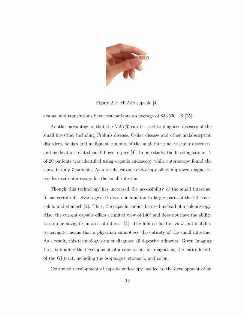
Figure 2.2: M2A r© capsule [4].
exams, and transfusions have cost patients an average of $33 630 US [15].
Another advantage is that the M2A r© can be used to diagnose diseases of the
small intestine, including Crohn’s disease, Celiac disease and other malabsorption
disorders, benign and malignant tumours of the small intestine, vascular disorders,
and medication-related small bowel injury [4]. In one study, the bleeding site in 12
of 20 patients was identified using capsule endoscopy while enteroscopy found the
cause in only 7 patients. As a result, capsule endoscopy offers improved diagnostic
results over enteroscopy for the small intestine.
Though this technology has increased the accessibility of the small intestine,
it has certain disadvantages. It does not function in larger parts of the GI tract,
colon, and stomach [2]. Thus, the capsule cannot be used instead of a colonoscopy.
Also, the current capsule offers a limited view of 140 and does not have the ability
to stop or navigate an area of interest [4]. The limited field of view and inability
to navigate means that a physician cannot see the entirety of the small intestine.
As a result, this technology cannot diagnose all digestive ailments. Given Imaging
Ltd. is funding the development of a camera pill for diagnosing the entire length
of the GI tract, including the esophagus, stomach, and colon.
Continued development of capsule endoscopy has led to the development of an
12
autonomous 9mm diameter by 23mm long capsule that is called the NORIKA3.
In addition to using peristaltic movement to navigate the digestive system, the
capsule uses a force generated by external electromagnetic fields to rotate. This
wireless tele-operated pill incorporates a charge-coupled device camera and some
drug-delivery modules for localized therapy [16]. Since chemical substances from
on-board batteries have the potential to damage the human body, an advantage of
the NORIKA3 over the M2A r© is that the power supplied to the NORIKA3 comes
from outside the body. Also, the capsule cost for the NORIKA3 alone is $120 US
while the M2A r© capsule costs $450 US [16]. However, this physician-guided device
will result in higher procedural costs since the physician needs to be present and
the patient hospitalised.
Different institutions are attempting to develop other systems that can be used
in the digestive tract. Though no commercial endoscopic inchworms are in exis-
tence, development by researchers is underway. Fox example, [11] proposes a robot
for colon inspection that has an outer diameter of approximately 15mm and a
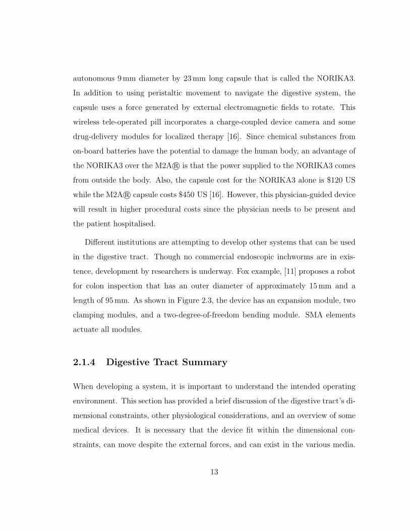
length of 95mm. As shown in Figure 2.3, the device has an expansion module, two
clamping modules, and a two-degree-of-freedom bending module. SMA elements
actuate all modules.
2.1.4 Digestive Tract Summary
When developing a system, it is important to understand the intended operating
environment. This section has provided a brief discussion of the digestive tract’s di-
mensional constraints, other physiological considerations, and an overview of some
medical devices. It is necessary that the device fit within the dimensional con-
straints, can move despite the external forces, and can exist in the various media.
13
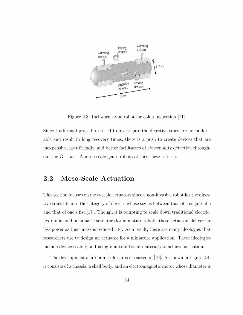
Figure 2.3: Inchworm-type robot for colon inspection [11].
Since traditional procedures used to investigate the digestive tract are uncomfort-
able and result in long recovery times, there is a push to create devices that are
inexpensive, user-friendly, and better facilitators of abnormality detection through-
out the GI tract. A meso-scale genre robot satisfies these criteria.
2.2 Meso-Scale Actuation
This section focuses on meso-scale actuators since a non-invasive robot for the diges-
tive tract fits into the category of devices whose size is between that of a sugar cube
and that of one’s fist [17]. Though it is tempting to scale down traditional electric,
hydraulic, and pneumatic actuators for miniature robots, these actuators deliver far
less power as their mass is reduced [18]. As a result, there are many ideologies that
researchers use to design an actuator for a miniature application. These ideologies
include device scaling and using non-traditional materials to achieve actuation.
The development of a 7mm-scale car is discussed in [19]. As shown in Figure 2.4,
it consists of a chassis, a shell body, and an electromagnetic motor whose diameter is
14
1.0mm. Since the car runs at a maximum speed of 100 mms
by electric power, wear of
the rotating parts is severe. Lubricant for the micro-rotating wheel bearings did not
help sufficiently due to the lubricant’s adhesive effect resulting from the relationship
between molecular force and surface tension [19]. Also, surface roughness severely
affects the movement of the device. Study of this system shows that factors may
affect smaller robots differently than traditional robots, and this makes it difficult
to miniaturize traditional robots by scaling. Since locomotion caused by a sliding or
rotating mechanism may not be suitable for micro-systems [19], alternate methods
of obtaining motion, such as electrically actuated polymer devices and piezoelectric
devices, are being developed by researchers.
Figure 2.4: Micro-fabricated car [20].
Electro-active polymers are a set of polymers actuated by electrical stimuli.
They are receiving attention as an alternative to existing actuators. One such actu-
ator under development is the ANTagonistically-driven Linear Actuator (ANTLA).
ANTLA comprises a polymer film and an elastomer film with affixed electrodes. By
15

varying the voltage of the electrodes, the actuator realises bi-directional actuation
in addition to compliance controllability [21]. Due to its simplicity of configura-
tion and ease of fabrication, it has the advantage of being scale independent [21].
Hence, its implementation in meso- and micro-scale applications shows potential.
According to [21], the device’s behaviour is difficult to model accurately due to the
related non-linear elastic coefficient and viscous properties.
A meso-scale robot using a piezoelectric-based locomotion technique that results
from amplification through a compliant mechanical structure is outlined in [22]. The
robot’s motion is a lift-and-pull scheme since voltage applied to the piezoelectric
element results in the legs causing a lifting motion while the removal of voltage
from the element causes the robot to pull forward. Figure 2.5 shows this slip/stick
locomotion.
Figure 2.5: Piezoelectric-based locomotion technique [22].
Potential advantages of piezo-based actuation methods versus miniaturized motor-
based approaches include a significantly increased power-to-volume ratio, reduced
cost, and increased accuracy [22]. However, this type of locomotion requires a
smooth surface since the actuator bends and slips when the voltage is applied,
16
but the actuator lengthens and sticks when the voltage is removed. This type of
locomotion can be considered only if speed is not a motivating factor. Also, the
piezoelectric actuated meso-scale mobile robot prototyped in [22] required a peak
amplitude of 100V for the applied voltage to achieve speeds of 65 cms
. The high
voltages required potentially pose a safety concern for application in the digestive
tract.
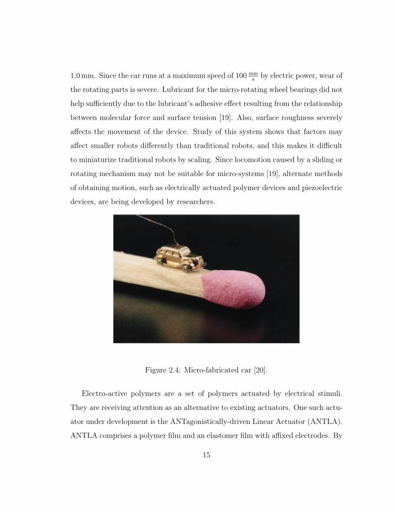
The successful testing of a proof-of-concept meso-scale actuator device contain-
ing micro-scale components is detailed in [23]. As seen in Figure 2.6, the proof-
of-concept device is similar to traditional piezoelectrically driven inchworm motors
except that mechanically interlocking micro-ridges replace the traditional frictional
clamping mechanisms. The intended purpose of the interlocked micro-ridges is to
increase the load carrying capability of the device since the strength of these micro-
ridges dictate the output force of the device. Unfortunately, it is necessary to apply
compensation during the locking and unlocking of the micro-ridges due to change
in the relative position of micro-ridges caused by external loads [23].
Figure 2.6: Meso-scale actuator with interlocking micro-ridges [23].
Another type of actuation used in meso-scale devices is electrostatic actuation.
17

Using electrostatic actuation to move its diaphragms, the dual-diaphragm pump
(DDP), as shown in Figure 2.7, shows promise to significantly advance gas pumping
at the micro- and meso-scale [24]. It has demonstrated bi-directional flow rates of
approximately 30 mLmin
with a power consumption of about 8mW. Its overall pump
volume is about 1.5×1.5×0.1 cm3. Three driving signals control the actuation of
the diaphragms. This fully scalable device is considered the most versatile and
the most efficient gas-pumping device at the micro- and meso-scale [24]. Typically,
the performance of miniature mechanical pumps are limited by their mechanical
components. One disadvantage of electrostatically actuated miniature pumps is
that they require high actuation voltages [25].
Figure 2.7: Schematic of dual-diaphragm pump [24].
Due to their size, meso-scale actuators have many promising applications. This
section provided a small sampling of the numerous actuators used in miniature
applications. SMAs are another type of material used in meso-scale actuators.
SMAs are described in more detail in the following section.
18
2.3 Shape Memory Alloys
Shape memory alloys (SMAs) are a type of material that researchers use to meet a
growing demand for lightweight, powerful actuators that can be scaled down. SMAs
display the shape memory effect (SME) when annealed appropriately. This effect
describes a material’s ability to return to a predetermined shape through heating
after being plastically deformed from that shape. Heating can be achieved through
Joule heating via electrical current.
A material’s properties dictate its use in an application. Since there are multiple
types of SMAs, including nickel titanium (NiTi), copper zinc aluminium (CuZnAl),
and copper aluminium nickel (CuAlNi), it is important to choose the most suitable
material for the intended application. In the proposed application, it is desired that
the SMA be heated via electrical current, that the SMA be biocompatible, and that
the SMA be scalable.
Thus for the intended application, a nickel-based SMA is preferable to a copper-
based SMA since greater Joule heating is achieved with the same current in a higher-
resistance material than in a lower-resistance material. As well, Nitinol, the NiTi
alloy, is an ideal material for medical applications due to its biocompatibility and its
ability to offer extremely high work-to-volume ratios when used as an actuator [26].
High work-to-volume ratios are significant since the low work-to-volume ratios of
most actuator technologies have limited micro-actuator development. This material
also has a reasonable cost and a great ability to recover large strains [18].
This section discusses the SME, SMA microscopic properties, phase transfor-
mation, SMA macroscopic behaviour, composite SMA actuator design, monolithic
SMA actuators, and biomedical applications that use SMA actuators.
19
2.3.1 Shape Memory Effect
The shape memory effect (SME) is a material’s ability to return to a predetermined
shape through heating after being plastically deformed from that shape. An SMA
in its cold-worked condition does not display the SME, but a shape-set anneal
will activate the SME in an SMA. A shape-set anneal is a process that requires
constraining the SMA in a desired shape and then performing a heat treatment.
This heat treatment must occur at a specific temperature and pressure for a certain
duration of time. A good reference to describe the shape-set anneal process is [27].
This reference is used for the development of the prototype in this work.
The heat treatment must ensure that the material reaches the desired temper-
ature while in the specified shape. Heating methods include the use of an air or
vacuum furnace, salt bath, sand bath, heated die, or laser. The method chosen de-
pends on the size of the SMA and equipment availability. Typically, the annealing
temperature is in the range of 450C to 550C [27]. Higher temperatures result in
lower tensile strengths. Since cooling should be rapid to avoid aging effects, a water
quench is recommended.
The time required for the heat treatment must be sufficiently long so that the
material reaches the desired temperature throughout its cross-section. Though
annealing times may be less than a minute for heating small parts in a salt bath
or heated die, they can be much longer for heating massive fixtures in a furnace
with an air or argon atmosphere. For the latter scenario, times of ten minutes to
twenty minutes are necessary. To produce the desired shape, experimentation for
the proper time and temperature is required.
20
2.3.2 Shape Memory Alloy Microscopic Properties
SMAs can display three distinct crystalline phases: austenite, martensite, and the
R-phase. In materials that exhibit the strongest SME, the R-phase is negligible
and hence will not be considered here [18]. The ability of an SMA to “remember”
a shape is contingent on its austenite and martensite phases. Since the microscopic
properties of these phases affect the macroscopic behaviour of an SMA device,
discussion of the microscopic structure is beneficial.
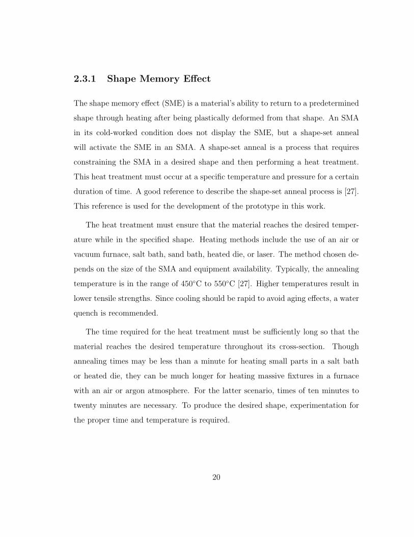
Austenite is the stronger, higher-temperature phase which has a crystalline mi-
croscopic structure that is usually body-centred cubic or a variant of body-centred
cubic. In a body-centred structure, there are atoms at each vertex of a cube and
one at the center [18]. Figure 2.8 shows this parent phase in a two-dimensional
schematic.
Figure 2.8: Austenite.
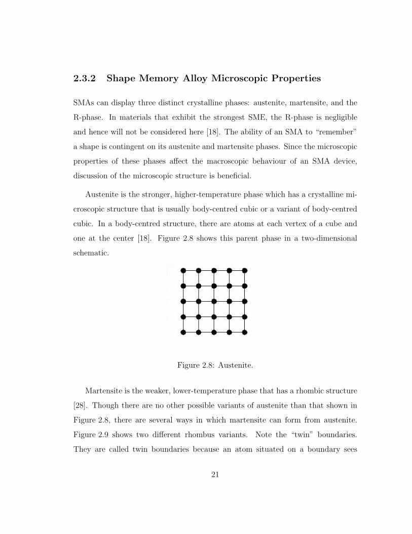
Martensite is the weaker, lower-temperature phase that has a rhombic structure
[28]. Though there are no other possible variants of austenite than that shown in
Figure 2.8, there are several ways in which martensite can form from austenite.
Figure 2.9 shows two different rhombus variants. Note the “twin” boundaries.
They are called twin boundaries because an atom situated on a boundary sees
21
mirror views on either side of the boundary [29]. While Figure 2.9 only shows the
two-dimensional representation of two variants, there are other possible variants.
Figure 2.9: Twinned martensite.
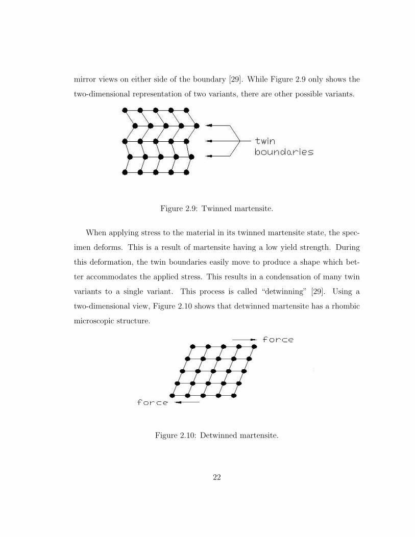
When applying stress to the material in its twinned martensite state, the spec-
imen deforms. This is a result of martensite having a low yield strength. During
this deformation, the twin boundaries easily move to produce a shape which bet-
ter accommodates the applied stress. This results in a condensation of many twin
variants to a single variant. This process is called “detwinning” [29]. Using a
two-dimensional view, Figure 2.10 shows that detwinned martensite has a rhombic
microscopic structure.
Figure 2.10: Detwinned martensite.
22
2.3.3 Phase Transformation
Unlike conventional materials, the transformation between austenite and martensite
is reversible and depends on the temperature of the SMA. Depending on whether
the material is transforming from martensite to austenite or from austenite to
martensite, different temperatures dictate the start and end of the transformation.
During the heating or cooling of the SMA, the history of the SMA affects the
material’s behaviour.
Temperatures
SMAs do not undergo their phase transformation from martensite to austenite or
from austenite to martensite at one specific temperature. The transformations be-
gin at one temperature and stop at another. These start and finish temperatures
are different depending on whether the material is heating or cooling. Thus, there
are four transition temperatures that indicate the start or finish of a martensite-to-
austenite or austenite-to-martensite transformation. In order of lowest to highest
temperature, they are TMf , TMs, TAs, and TAf . The following transformation de-
scription indicates what occurs at each temperature.
Assume that a strip of SMA begins at an initial temperature where it is com-
pletely martensite. Increasing the temperature to TAs will cause the material to
start transforming to austenite. Once the temperature reaches TAf , the material is
completely austenite. If unconstrained, the material resumes its memorized shape
since austenite only exists as a cubic lattice at this stage.
Assume that a strip of SMA begins at an initial temperature where it is com-
pletely austenite. Decreasing the temperature to TMs causes the material to start
transforming to martensite. Once the temperature is cooled to TMf , the material is
23

completely twinned martensite which does not entail a change in shape if unloaded.
The martensite is twinned since it was constrained by the surrounding crystal lattice
to maintain the austenite shape during the martensitic transformation [18].
Figure 2.11 shows the transformation temperatures and their relation to marten-
site and austenite in the material. Though the transformation temperatures are
intended to indicate precisely where transformations begin and end, for the pur-
poses of modelling and simulation in this work, these temperatures occur at the
intersection of the plateau and sloped lines representing the heating and cooling
curves. It is common practice to define the transformation temperatures as shown
in Figure 2.11 since it is very difficult to gauge experimentally exactly when the
material starts or finishes changing phases. Correspondingly, it is expected that the
simulations will show that the material begins transforming before the transforma-
tion start temperatures and will continue transforming after the transformation
finish temperatures.
In the intended application, it is crucial that the transition temperatures cor-
respond with temperatures suitable for use in the body. The ratio of nickel and
titanium dictate the transformation temperatures. Since the transformation tem-
peratures are sensitive to small alloy composition changes, a 1% shift in the amount
of either nickel or titanium in the alloy results in a 100C change in TAf [30]. Cor-
respondingly, it is necessary to control the alloy composition within ± 0.05% if it is
desired to control the alloy transformation temperatures within ± 5C [30]. Accord-
ing to [30], the family of typical commercial Nitinol alloys cover an TAf range from
approximately 100C with a nickel:titanium atomic ratio of about 50:50 to about
-20C with a nickel:titanium atomic ratio of about 51.2:48.8. Typical tolerances for
TAf are ± 3C to ± 5C [27]. Typically, TAs is approximately 15C to 20C lower
than TAf , and TMf is about 15C to 20C lower than TMs [27].
24

Figure 2.11: Transformation temperatures. TMs is the martensite start tempera-
ture. TMf is the martensite finish temperature. TAs is the austenite start temper-
ature. TAf is the austenite finish temperature.
25
Hysteresis
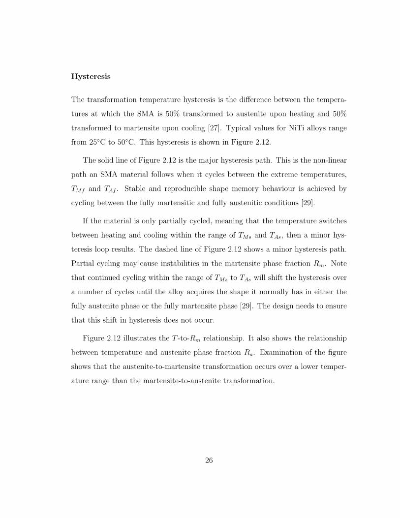
The transformation temperature hysteresis is the difference between the tempera-
tures at which the SMA is 50% transformed to austenite upon heating and 50%
transformed to martensite upon cooling [27]. Typical values for NiTi alloys range
from 25C to 50C. This hysteresis is shown in Figure 2.12.
The solid line of Figure 2.12 is the major hysteresis path. This is the non-linear
path an SMA material follows when it cycles between the extreme temperatures,
TMf and TAf . Stable and reproducible shape memory behaviour is achieved by
cycling between the fully martensitic and fully austenitic conditions [29].
If the material is only partially cycled, meaning that the temperature switches
between heating and cooling within the range of TMs and TAs, then a minor hys-
teresis loop results. The dashed line of Figure 2.12 shows a minor hysteresis path.
Partial cycling may cause instabilities in the martensite phase fraction Rm. Note
that continued cycling within the range of TMs to TAs will shift the hysteresis over
a number of cycles until the alloy acquires the shape it normally has in either the
fully austenite phase or the fully martensite phase [29]. The design needs to ensure
that this shift in hysteresis does not occur.
Figure 2.12 illustrates the T -to-Rm relationship. It also shows the relationship
between temperature and austenite phase fraction Ra. Examination of the figure
shows that the austenite-to-martensite transformation occurs over a lower temper-
ature range than the martensite-to-austenite transformation.
26
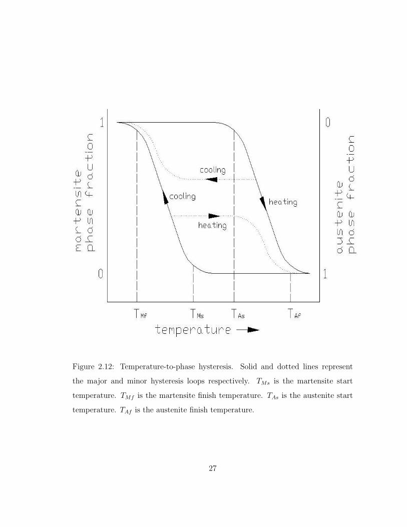
Figure 2.12: Temperature-to-phase hysteresis. Solid and dotted lines represent
the major and minor hysteresis loops respectively. TMs is the martensite start
temperature. TMf is the martensite finish temperature. TAs is the austenite start
temperature. TAf is the austenite finish temperature.
27

2.3.4 Shape Memory Alloy Macroscopic Behaviour
Many SMA properties depend on temperature and affect the macroscopic behaviour
of the SMA. These temperature-dependent properties include electrical resistance,
latent heat of transformation, magnetic properties, thermal conductivity, damping,
roughness, colour, hardness, and sound [29]. Other properties, such as transforma-
tion temperatures, depend on the applied stress [18]. A discussion of the unloaded
and loaded performance of an SMA follows an overview of the relationship between
stress, strain, and temperature in an SMA.
Stress-Strain-Temperature Relationship
The stress, strain, and temperature of an SMA are interdependent. Since the
SMA stress-strain relationship depends on temperature, the Young’s modulus also
depends on temperature. Young’s modulus is the ratio of the applied stress to
the resulting strain. Figure 2.13 shows two curves. One curve corresponds to the
material in its fully martensitic state while the other curve corresponds to the
material in its austenitic state.
There are piece-wise continuous segments that describe the martensite stress-
strain relationship. Assume that initially the SMA material is fully twinned marten-
site with a temperature below TMf . The linear portion prior to (a) corresponds to
the elastic operating range of the SMA. When loading in this region, stress increases
linearly with strain. The Young’s modulus is Em,l in the linear region. After the
first yield point, there is an approximate plateau, from (a) to (b), where a small
change in stress results in a significant change in strain. This process is called
detwinning. At this stage, an externally applied stress can force all variants of the
martensite into a single variant. If the external stress is removed, the martensite
28
Figure 2.13: SMA stress-strain curves. The high-temperature curve corresponds
with TAf while the low-temperature curve corresponds with TMf . At (a), the de-
twinning of martensite begins. At (b), the martensite is fully detwinned. At (c),
detwinned martensite deforms elastically. At (d), slip begins to occur and perma-
nent deformation results. Martensite detwinning begins at εmy while εm
d is the
strain where the martensite becomes fully detwinned. Adapted from [18] and [31].
29
will recover slightly, but it will remain deformed. The Young’s modulus is Em,t from
(a) to (b) where the material is detwinning. Point (c) indicates an elastic region
where the atomic bonds within the rhombic crystalline structure can be stretched.
If the stress is removed, the martensite will return to its fully detwinned form. Em,d
is the Young’s modulus in the elastic region corresponding to point (c). Applying
too much stress leads to slip. At point (d), atomic bonds break and permanent, ir-
recoverable deformation occurs. The strain where detwinning of martensite begins
is εmy while εm
d is the strain where the martensite becomes fully detwinned. For
more detail, see [18].
The high-temperature SMA curve has a greater slope and hence a greater
Young’s modulus than the low-temperature SMA curve. The Young’s modulus is
Ea. Therefore, an SMA device is capable of exerting a greater force in its austenitic
state than in its martensitic state.
Unloaded Shape Memory Alloy Behaviour
Figure 2.14 illustrates cycling between austenite and martensite microscopically
and macroscopically for an SMA cantilever beam. While considering this example,
assume that the beam’s memorized shape is flat.
Assume that the beam begins at an initial temperature where it is completely
martensite [Figure 2.14 (a)]. Applying a load at the tip of the beam causes it to
deform. After removing the load, the beam remains deformed [Figure 2.14 (b)].
Increasing the temperature to TAs causes the material to start transforming from
martensite to austenite. Once the temperature reaches TAf , the beam is completely
austenite. The beam will resume its original shape [Figure 2.14 (c)].
Now assume that the SMA beam begins at an initial temperature where it is
30
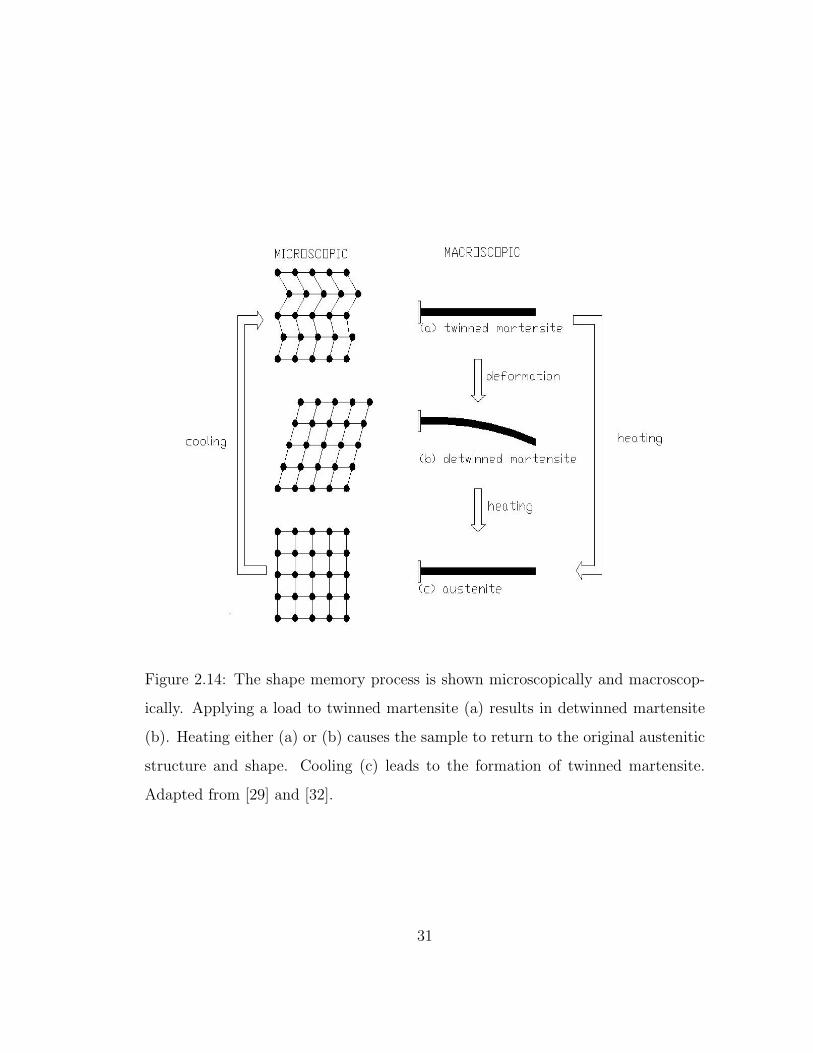
Figure 2.14: The shape memory process is shown microscopically and macroscop-
ically. Applying a load to twinned martensite (a) results in detwinned martensite
(b). Heating either (a) or (b) causes the sample to return to the original austenitic
structure and shape. Cooling (c) leads to the formation of twinned martensite.
Adapted from [29] and [32].
31
completely austenite [Figure 2.14 (c)]. Decreasing the temperature to TMs causes
the material to start transforming to martensite. Once the temperature is cooled
to TMf , the SMA beam is completely twinned martensite [Figure 2.14 (a)]. The
macroscopic shape of the beam at both phases is the same.
If the beam begins at an initial temperature where it is completely martensite
[Figure 2.14 (a)] and is heated to TAf , the beam will be completely austenite and
will not change shape as it changes phase [Figure 2.14 (c)].
Loaded Shape Memory Alloy Behaviour
Figure 2.15 illustrates the macroscopic effect of applying force in two stages to a
cantilever beam that cycles between austenite and martensite. One force is a con-
stant load applied at the free end while the other force is applied and removed at the
free end. As will be seen later on, the proposed actuator incorporates this behaviour
of applying force in multiple stages. For this example, the beam’s memorized shape
is flat and gravity acts in the direction of deflection.
Assume that the beam begins at an initial temperature where it is completely
twinned martensite [Figure 2.15 (a)]. The beam is then fixed at one end and a
constant load is applied to the free end [Figure 2.15 (b)]. The beam’s free end is
a distance d(b) from its unloaded position. In this configuration, the martensite
starts to detwin. Between (b) and (c) of Figure 2.15, an additional external load is
applied and then removed. This causes the beam to deform further in the direction
of gravity and to become fully detwinned martensite. The tip displacement is
d(c). Note that d(c) is greater than d(b). Heat is then applied to the beam with
its constant load. Increasing the temperature to TAs causes the material to start
transforming from martensite to austenite. As the beam transforms, it attempts
32

Figure 2.15: Loaded SMA macroscopic behaviour.
33
to resume its memorized shape. Once the temperature reaches TAf , the beam is
completely austenite. However, the constant load impedes the beam from achieving
its memorized shape. The tip deflection is d(d) [Figure 2.15 (d)]. Note that d(d) is less
than d(b). Removing the constant load while continuing to maintain the temperature
of the beam at TAf causes the beam to resume its original shape [Figure 2.15 (e)].
2.3.5 Shape Memory Alloy Actuator Design
If treated to display the SME, an SMA will generate extremely large forces if it
encounters any resistance while transforming from martensite to austenite. By
using the SMA’s increase in strength with temperature in a design, SMA actuators
can perform useful work. Consider the example of an SMA spring under constant
load illustrated in Figure 2.16.
At low temperature, an SMA spring loaded with a mass m deflects a distance
dl following line OB due to the force of gravity ~g. When the temperature increases,
the same spring with the same load deflects a distance dh following line OA. Thus
as the temperature increases, the system performs work equivalent to the product
mg(dl−dh) [29]. This system is self-resetting because the weight naturally stretches
the spring at low temperature.
As seen in Figure 2.17, sometimes a spring made with conventional material,
such as steel, provides a bias force to reset the SMA spring at a lower tempera-
ture. The SMA spring works against the increasing force of the bias spring. As
the temperature of the SMA spring increases so does its strength. Thus at high
temperature, the SMA spring will exert a greater force [Figure 2.17 (b)] on the bias
spring than at low temperature [Figure 2.17 (a)]. The displacement difference of
the rod at the two extreme temperatures is the obtained motion ∆x.
34
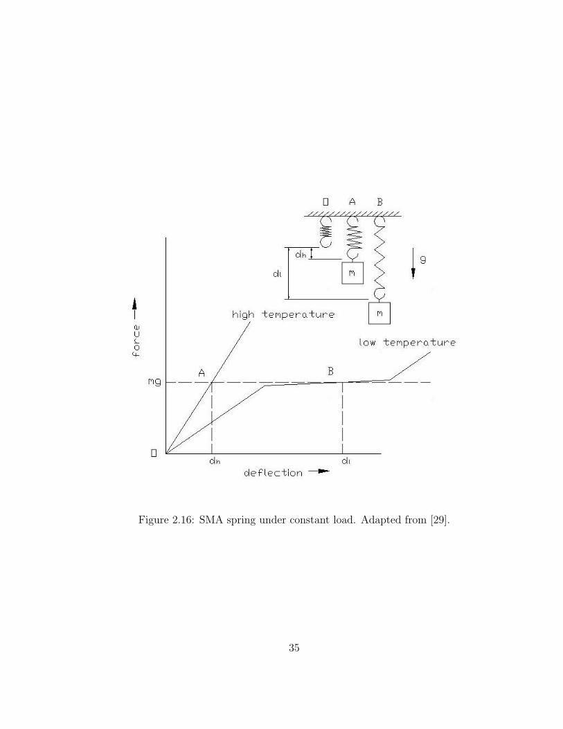
Figure 2.16: SMA spring under constant load. Adapted from [29].
35
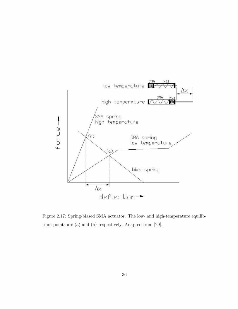
Figure 2.17: Spring-biased SMA actuator. The low- and high-temperature equilib-
rium points are (a) and (b) respectively. Adapted from [29].
36

In the example shown in Figure 2.17, the SMA-actuated piston is not loaded.
If the piston is loaded, as shown in Figure 2.18, the amount of displacement ∆x
decreases since the new high-temperature equilibrium point [Figure 2.18 (b’)] occurs
where the sum of the force of the bias spring and the load equal the force of the
SMA spring. Hence, ∆F is the net force which the SMA-actuated piston can exert
on a load mg after a displacement ∆x.
Figure 2.18: Spring-biased SMA actuator with external load. The low- and high-
temperature equilibrium points are (a) and (b) respectively. Adapted from [29].
37
2.3.6 Monolithic Shape Memory Alloy Actuator
SMA actuators require a bias force for reset in order to obtain cyclic motion. The
use of discrete masses or bias springs for this purpose is more difficult as devices are
miniaturized. Instead of using a biasing device made from a conventional material
for the reset force, it is possible to create a monolithic SMA device by locally
treating certain regions. Monolithic actuators are single-piece mechanical devices
that move something. The annealed regions of a monolithic device exhibit the
SME while the remaining non-annealed parts demonstrate elastic behaviour. The
non-annealed parts act as the bias force. Hence, monolithic SMA devices integrate
the bias force and reset mechanism within the same piece of material. There are
different ways to locally anneal a structure. They include direct Joule heating of
the material and laser heating.
In direct heating, the material is heated up to its annealing temperature using a
high current. The work in [33] demonstrated this as an efficient method by applying
it to a one-axis translation stage shown in Figure 2.19. Using a laser, the structure
was cut from a non-annealed SMA strip. The left springs were then annealed
by applying a current through them. Following the cooling of the structure, the
right and left springs were pre-strained along the x-direction as indicated in the
figure. The mechanism moves as the left springs transform to and from austenite.
When the left springs become austenite, they recover their initial shape and pull the
moving part to the left. The stage is pulled to the right because of the non-annealed
springs when the left springs cool.
Though direct heating works, there are problems associated with this technique
including the requirement for an electrical path in the design and the necessity
for careful consideration of the structure thickness with respect to temperature
38
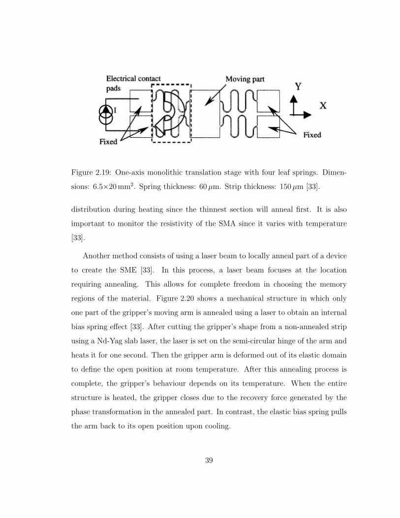
Figure 2.19: One-axis monolithic translation stage with four leaf springs. Dimen-
sions: 6.5×20mm2. Spring thickness: 60µm. Strip thickness: 150µm [33].
distribution during heating since the thinnest section will anneal first. It is also
important to monitor the resistivity of the SMA since it varies with temperature
[33].
Another method consists of using a laser beam to locally anneal part of a device
to create the SME [33]. In this process, a laser beam focuses at the location
requiring annealing. This allows for complete freedom in choosing the memory
regions of the material. Figure 2.20 shows a mechanical structure in which only
one part of the gripper’s moving arm is annealed using a laser to obtain an internal
bias spring effect [33]. After cutting the gripper’s shape from a non-annealed strip
using a Nd-Yag slab laser, the laser is set on the semi-circular hinge of the arm and
heats it for one second. Then the gripper arm is deformed out of its elastic domain
to define the open position at room temperature. After this annealing process is
complete, the gripper’s behaviour depends on its temperature. When the entire
structure is heated, the gripper closes due to the recovery force generated by the
phase transformation in the annealed part. In contrast, the elastic bias spring pulls
the arm back to its open position upon cooling.
39
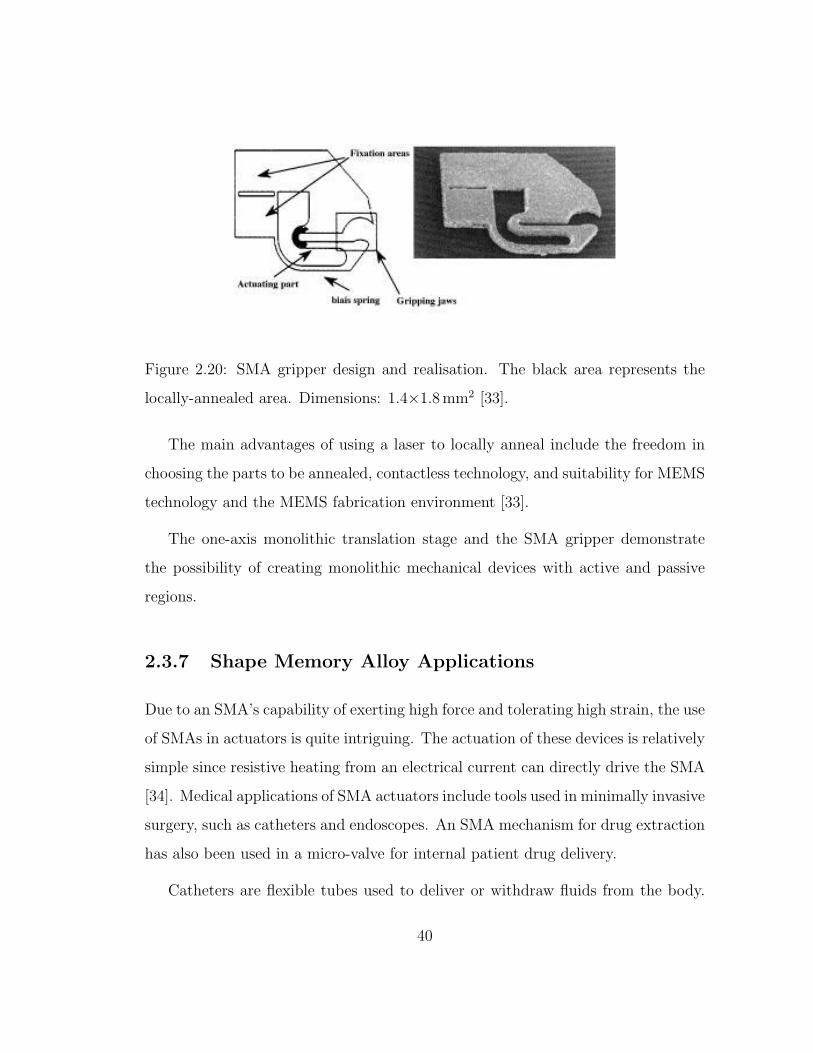
Figure 2.20: SMA gripper design and realisation. The black area represents the
locally-annealed area. Dimensions: 1.4×1.8mm2 [33].
The main advantages of using a laser to locally anneal include the freedom in
choosing the parts to be annealed, contactless technology, and suitability for MEMS
technology and the MEMS fabrication environment [33].
The one-axis monolithic translation stage and the SMA gripper demonstrate
the possibility of creating monolithic mechanical devices with active and passive
regions.
2.3.7 Shape Memory Alloy Applications
Due to an SMA’s capability of exerting high force and tolerating high strain, the use
of SMAs in actuators is quite intriguing. The actuation of these devices is relatively
simple since resistive heating from an electrical current can directly drive the SMA
[34]. Medical applications of SMA actuators include tools used in minimally invasive
surgery, such as catheters and endoscopes. An SMA mechanism for drug extraction
has also been used in a micro-valve for internal patient drug delivery.
Catheters are flexible tubes used to deliver or withdraw fluids from the body.
40

An active catheter which has a bending mechanism realised by thin NiTi SMA
plates has been developed and commercialised [35]. As seen in Figure 2.21, there
are active catheters that comprise several sensors and a multi-joint mechanism with
distributed NiTi SMA actuators to enable bending, torsion, and extension depend-
ing on the configuration of the SMA actuators and bias springs in development.
Figure 2.21: Bending, torsional, and extending active catheter using SMA coil
actuators [35].
The catheter has an outer diameter of 1.4mm. There are also active guide wires
that have diameters of 0.5mm. The devices are fabricated at low cost using micro-
machining and are disposable [36]. These SMA mechanisms facilitate minimally
invasive diagnosis and therapy while reducing patient discomfort.
Colonoscopies enable the examination of the rectum and colon. Typically, doc-
tors use a long, flexible tube with a light and a tiny lens at the tip. Unfortunately,
conventional devices for this complex procedure are quite rigid. This results in
patient distress and increases the complexity of the procedure. As a result, there is
on-going research to design and fabricate a micro-robot capable of propelling semi-
autonomously along the colon. One such system’s actuation system is based on
41

SMA pneumatic micro-valves that utilise the inchworm locomotion technique. In
this technique, pneumatic actuators clamp to the colon walls while other pneumatic
actuators provide extension in order to obtain motion [37]. No accurate theoretical
model currently exists to predict the colon tissue behaviour during its interaction
with the micro-robot. Consequently, a model of the human colon was created us-
ing animal tissues in the lab. Favourable preliminary results using animal tissues
illustrate the feasibility of the micro-robot.
Daily drug injections are mandatory for many people with various medical con-
ditions. An actively controlled drug delivery device implanted in the body would re-
duce the necessity for skin perforations. The operating principle of the implantable
drug delivery device of [26] is based on a precisely controlled, discontinuous release
from a pressurized reservoir using an SMA actuator. The application of resistive
heating induces the contraction of the SMA element. Correspondingly, the tube
opens and the drug is dispensed. When the SMA cools, the valve closes due to the
elasticity of the joint. Remote control of the device is possible since a transformer
transmits control signals and power through the skin [26]. This simple actuation
technology relies on the SME for actuation. The utilisation of SMAs reduces the
number of parts since an SMA element replaces a classic hinged joint by an elastic
joint, and it removes the need for a motor or other actuator.
2.3.8 Shape Memory Alloy Summary
To understand the proposed actuator in the next chapter, it is critical to understand
the material and its potential. NiTi is a biocompatible SMA that displays the SME
when properly processed.
While shifting from its low-temperature phase to its high-temperature phase,
42

and thus returning to its original shape, a properly heat-treated SMA exerts a force
against anything that opposes its movement. Locally annealing an SMA leads to
a mechanism with active and passive parts that can work together to create a
monolithic actuator that allows for miniaturization. The next chapter uses the
SMA background information to develop and model a monolithic actuator using
NiTi.
43
Chapter 3
Analytical Model Development
To understand the actuator’s behaviour before costly prototyping, it is useful to
model the system. After introducing the proposed geometry, the objective of this
chapter is to derive a model for use in simulation and design.
3.1 Proposed Geometry
Before modelling the system, it is necessary to introduce the proposed geometry.
Every leg of the six-legged robot illustrated in Figure 1.1 incorporates two actua-
tors, each made from one piece of SMA. Figure 3.1 displays one of the monolithic
actuators. The hatched region indicates the annealed area. This middle compo-
nent displays the SME. The non-hatched region corresponds to the area known as
the portal. Note that the section of the portal which attaches the non-annealed
cantilever beams with the annealed beam at the free end is called the girder.
To understand the tip displacement as a function of temperature, assume that
the middle beam can be detached from the portal. The memorized shape of the
44

Figure 3.1: Proposed actuator design. The hatched region indicates the area capa-
ble of exhibiting the SME. The non-hatched region corresponds to the area known
as the portal.
middle beam is a curved beam [Figure 3.2 (a)]. When detached from the portal,
there is no bias load acting on the beam. It will be in the same curved position
regardless of whether it is martensite or austenite. The portal is originally flat and
does not display the SME [Figure 3.2 (d)]. Let T be the temperature of the middle
beam. Now attach the middle beam and the portal at T ≤ TMf . At T ≤ TMf ,
the middle beam is martensite and in its weaker state. The tip of the actuator will
settle at some low-temperature equilibrium position between the memorized curved
position of the middle beam and the flat position of the portal [Figure 3.2 (c)]. If the
temperature of the middle beam increases, the amount of austenite in the middle
beam increases. As the amount of austenite in the middle beam increases, the
middle beam will move toward its memorized shape. When TAf ≤ T , the middle
beam will be completely austenite and the tip of the actuator will settle at some
high-temperature equilibrium position [Figure 3.2 (b)]. By cycling the temperature
between T ≤ TMf and TAf ≤ T , the tip of the actuator will move between the low-
temperature equilibrium position and the high-temperature equilibrium position.
45
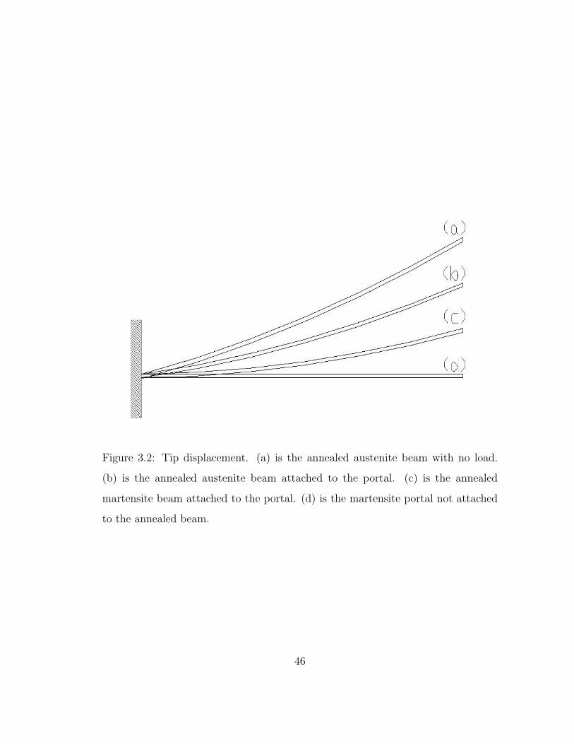
Figure 3.2: Tip displacement. (a) is the annealed austenite beam with no load.
(b) is the annealed austenite beam attached to the portal. (c) is the annealed
martensite beam attached to the portal. (d) is the martensite portal not attached
to the annealed beam.
46

The length, width, and thickness of the annealed beam are Lb, bb, and tb re-
spectively. The length, width, and thickness of the cantilevers of the non-annealed
portal are LAB, bAB, and tAB respectively. The length, width, and thickness of the
girder are LBC , bBC , and tBC respectively.
At low temperature, the portal acts as a biasing force to pull the middle beam
from its original shape. The annealed beam curves upward when heated because
its austenite shape is an upward-curved beam. Thus at high temperature, the
beam lifts the portal. By varying the current through the actuator, and hence its
temperature, the annealed middle beam and the non-annealed portal work together
to facilitate the required locomotion.
3.2 System Model
Two predominant modelling methods are distributed element and lumped element.
In a distributed element model, a partial differential equation, in which both time
and space are independent variables, describes the system. In a lumped model, the
physical parameter is lumped at one point. It uses an ordinary differential equation
in which time is the independent variable. For this preliminary actuator design,
the analytical equations for the lumped model of the actuator’s end-point deflection
will be developed using current as the system input.
Now that the type of model has been chosen, it is important to choose the
model components. Typical components used to model a system that has repetitive
motion are masses, springs, and dampers. The motion of a mass mx with changing
velocity is determined by the net force acting on the mass [38]. A spring, with
spring constant kx , is a physical model for storing energy. Its associated force is
related to displacement. A damper, with damping coefficient cx, is a physical model
47
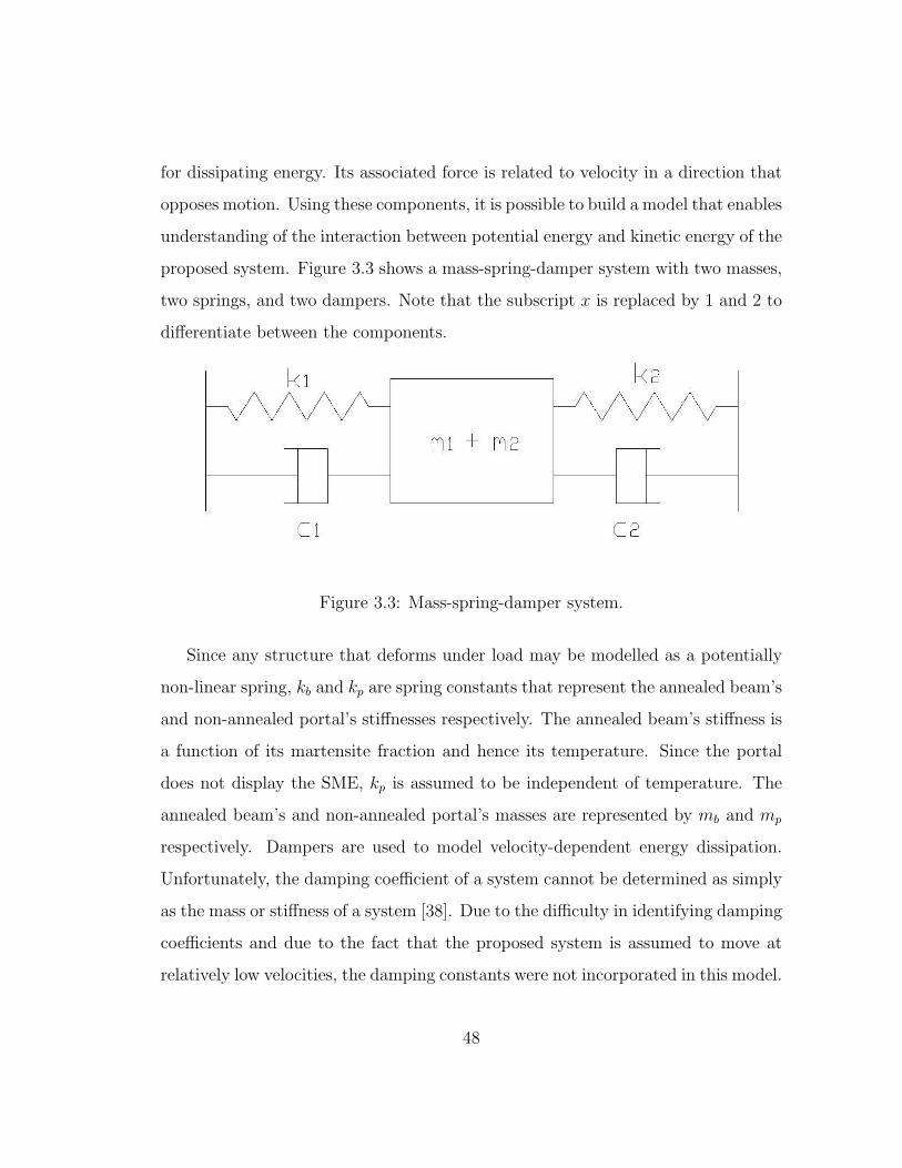
for dissipating energy. Its associated force is related to velocity in a direction that
opposes motion. Using these components, it is possible to build a model that enables
understanding of the interaction between potential energy and kinetic energy of the
proposed system. Figure 3.3 shows a mass-spring-damper system with two masses,
two springs, and two dampers. Note that the subscript x is replaced by 1 and 2 to
differentiate between the components.
Figure 3.3: Mass-spring-damper system.
Since any structure that deforms under load may be modelled as a potentially
non-linear spring, kb and kp are spring constants that represent the annealed beam’s
and non-annealed portal’s stiffnesses respectively. The annealed beam’s stiffness is
a function of its martensite fraction and hence its temperature. Since the portal
does not display the SME, kp is assumed to be independent of temperature. The
annealed beam’s and non-annealed portal’s masses are represented by mb and mp
respectively. Dampers are used to model velocity-dependent energy dissipation.
Unfortunately, the damping coefficient of a system cannot be determined as simply
as the mass or stiffness of a system [38]. Due to the difficulty in identifying damping
coefficients and due to the fact that the proposed system is assumed to move at
relatively low velocities, the damping constants were not incorporated in this model.
48

Hence, this chapter develops the expressions for equivalent stiffnesses and masses
alone. Figure 3.4 shows the proposed actuator design and its equivalent lumped
model. In the lumped system model, the annealed beam and non-annealed portal
lumped masses are in series with the equivalent lumped springs.
Figure 3.4: Proposed actuator design (left) and its equivalent lumped model (right).
The hatched region indicates the annealed region. The annealed beam’s stiffness
kb is a function of the annealed beam’s temperature T .
Two system block diagrams are developed. One assumes that the relationship
between temperature and Young’s modulus is linear during transformation while
the other better models the non-linear behaviour relating temperature and Young’s
modulus. The former is referred to as the linear Young’s modulus system model
while the latter is referred to as the non-linear Young’s modulus system model.
The remainder of this chapter includes the detailed derivation of the components
in the models.
The block diagram for the linear Young’s modulus system model is shown in
Figure 3.5. It presents the different model components chosen to develop an ex-
pression that relates the input current I to the annealed beam end-point deflection
yb assuming a linear relationship between the Young’s modulus of the middle beam
49
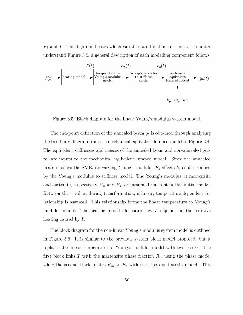
Eb and T . This figure indicates which variables are functions of time t. To better
understand Figure 3.5, a general description of each modelling component follows.
kp, mp, mb
mechanicalequivalent
lumped modelyb(t)I(t) heating model
T (t)
temperature toYoung’s modulus
model
Eb(t)
model
kb(t)
Young’s modulusto stiffness
Figure 3.5: Block diagram for the linear Young’s modulus system model.
The end-point deflection of the annealed beam yb is obtained through analysing
the free-body diagram from the mechanical equivalent lumped model of Figure 3.4.
The equivalent stiffnesses and masses of the annealed beam and non-annealed por-
tal are inputs to the mechanical equivalent lumped model. Since the annealed
beam displays the SME, its varying Young’s modulus Eb affects kb as determined
by the Young’s modulus to stiffness model. The Young’s modulus at martensite
and austenite, respectively Em and Ea, are assumed constant in this initial model.
Between these values during transformation, a linear, temperature-dependent re-
lationship is assumed. This relationship forms the linear temperature to Young’s
modulus model. The heating model illustrates how T depends on the resistive
heating caused by I.
The block diagram for the non-linear Young’s modulus system model is outlined
in Figure 3.6. It is similar to the previous system block model proposed, but it
replaces the linear temperature to Young’s modulus model with two blocks. The
first block links T with the martensite phase fraction Rm using the phase model
while the second block relates Rm to Eb with the stress and strain model. This
50

block diagram models the hysteresis in the temperature-strain and strain-stress
relationships. This non-linear behaviour increases the difficulty of modelling the
system.
I(t)
T (t)
modelmodelheating phase
stressand
strainmodel model
mechanicalequivalentlumpedmodel
kb(t)Eb(t)Rm(t)
Young’smodulus
to stiffness
kp, mp, mb
yb(t)
Figure 3.6: Block diagram for the non-linear Young’s modulus system model.
3.3 Mechanical Equivalent Lumped Model
Since the annealed beam’s stiffness kb(T ) is a function of temperature, changing
the annealed beam’s temperature causes the system’s tip deflection yb to vary.
Figure 3.7 displays the coordinate system used to define the tip’s displacement.
At T ≤ TMf and TAf ≤ T , the tip displacement is yb,l and yb,h respectively. The
distance between the annealed austenite beam with no load [Figure 3.7 (a)] and
the non-annealed portal with no load [Figure 3.7 (d)] is yflat. Note that detach-
ing the annealed austenite beam and the non-annealed portal can only be done
conceptually.
Figure 3.8 illustrates the coordinate system with the equivalent lumped model.
Note that no external force, including gravity, is incorporated in this model. The
free-body diagram of Figure 3.8 is shown in Figure 3.9.
51

Figure 3.7: Coordinate system showing tip displacement. (a) is the annealed
austenite beam with no load. (b) is the annealed austenite beam attached to
the portal. (c) is the annealed martensite beam attached to the portal. (d) is the
non-annealed portal not attached to the annealed beam.
yb = yflat
mb + mp
kpkb(T )
yb
yb = yb,hyb = 0 yb = yb,l
Figure 3.8: Mechanical equivalent lumped model.
52

Fp
kb(T )
mb + mp
kp
Fb = kbyb Fp = kp(yflat − yb)
Fb
Figure 3.9: Free-body diagram of mechanical equivalent lumped model.
Since the sum of forces must equal the product of mass and acceleration,
analysing the free-body diagram leads to the dynamic equation (3.1).
(mb + mp)yb + (kb(T ) + kp) yb − kpyflat = 0 (3.1)
At displacements yb = yb,l and yb = yb,h, yb = 0. Solving (3.1) at these points
gives expressions for yb,l (3.2) and yb,h (3.3).
yb,l =kpyflat
kb,l + kp
(3.2)
yb,h =kpyflat
kb,h + kp
(3.3)
The difference between yb,l (3.2) and yb,h (3.3) is the desired tip deflection ytip
(3.4).
ytip =
(kp
kb,l + kp
− kp
kb,h + kp
)yflat (3.4)
3.4 Equivalent Stiffness of Annealed Beam
To determine the equivalent lumped model of a system, it is necessary to calcu-
late the components’ equivalent stiffnesses and masses. This section focuses on
53

determining the annealed beam’s equivalent stiffness.
Beams are slender members that support loadings perpendicularly applied to
their longitudinal axis [8]. It is possible to treat the non-annealed portal as an
applied load to the annealed beam by ensuring that the displacements at the tip
of the annealed beam and at the mid-point of the girder are equal. Compatability
requires this since these spots physically correspond to the same location on the
piece of NiTi. The load created by the portal on the annealed beam varies as the
temperature changes. For example, the load caused by the portal increases as yb
decreases toward yb,h from yb,l.
It is necessary to establish the Eb-to-kb, Rm-to-Eb, T -to-Rm, and I-to-T relation-
ships. SMAs exhibit significant hysteresis in the temperature-strain, strain-stress,
and temperature-resistance relationships [18]. This non-linear behaviour increases
the difficulty of modelling the system.
3.4.1 Young’s Modulus to Stiffness Model
To determine the relationship between the annealed beam’s equivalent stiffness kb
and its Young’s modulus Eb, [8] and [39] were used.
Given the curved cantilever beam in Figure 3.10, kb is approximated using the
elastic curve of a flat cantilever beam with an end-point load while assuming the
curved beam’s radius of curvature is not significant. This assumption is a good
approximation if the tip displacement is less than 7% of the beam’s length. If much
greater movement is desired, the tip displacement can be increased, but then the
elastic curve for a curved cantilever beam should be used.
For the annealed cantilever beam with a second moment of area Ib = bbtb3
12, its
tip deflection yb due to an end-point load F is:
54

Figure 3.10: Curved cantilever beam with end-point load.
yb =Lb
3
3EbIb
F (3.5)
Hence, the equivalent stiffness kb of a spring modelling the behaviour of the
annealed beam at its tip is:
kb(T ) =3Eb(T )Ib
Lb3 (3.6)
3.4.2 Linear Temperature to Young’s Modulus Model
The linear Young’s modulus system model uses a linear approximation that ignores
hysteresis to describe the relationship between the temperature of the annealed
beam T and the Young’s modulus of the annealed beam Eb. The Young’s modulus
at martensite and austenite, respectively Em,l and Ea, are assumed constant in this
linear model. Between these values during transformation, a linear relationship
is used to relate T and Eb. Outside the transformation temperature range, the
modulus saturates at the appropriate value. Note that (3.7) is not valid if the
temperature exceeds the temperature at which the SMA is annealed Tanneal.
55

Eb(T ) =
Em,l T < TMf
(Ea−Em,l
TAf−TMf
)T +
(Em,l −
(Ea−Em,l
TAf−TMf
)TMf
)TMf ≤ T ≤ TAf
Ea TAf < T
(3.7)
3.4.3 Stress and Strain Model
The non-linear Young’s modulus system model relates the martensite fraction Rm
to Eb with the stress and strain model. As shown in (3.8), Eb depends on the stress
σ and strain ε of the annealed beam in this model.
Eb =σ
ε(3.8)
In conventional materials, the Young’s modulus is only marginally affected by
temperature [31]. However, the strain-to-stress relationship for SMAs has a strong
temperature dependence due to the relationship between temperature and phase
fraction.
Stress Model
The material’s total stress depends on the crystalline phase fractions. As shown
in Figure 2.12, which is shown again in Figure 3.11 for the reader’s convenience,
there is a temperature range over which both austenite and martensite coexist in
the solid. Microscopically, these phases are distributed randomly throughout the
material. However from a macroscopic point of view, it is possible to treat the
phases as sublayers connected in parallel [40].
56

Figure 3.11: Temperature-to-phase hysteresis. Solid and dotted lines represent
the major and minor hysteresis loops respectively. TMs is the martensite start
temperature. TMf is the martensite finish temperature. TAs is the austenite start
temperature. TAf is the austenite finish temperature.
57
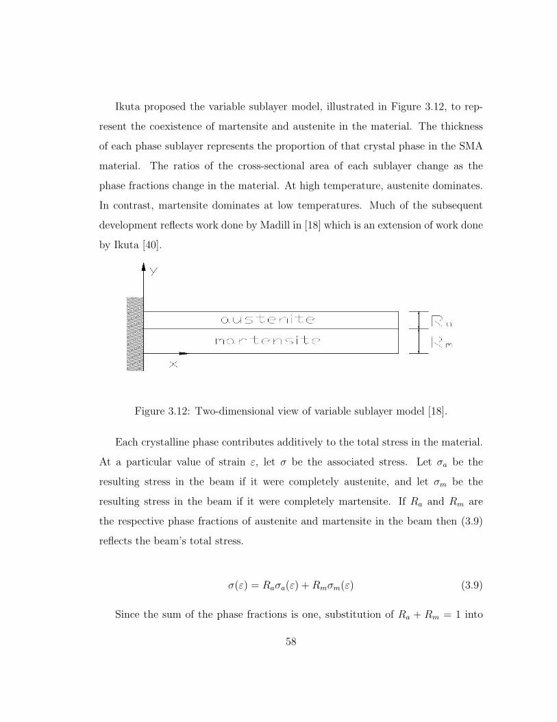
Ikuta proposed the variable sublayer model, illustrated in Figure 3.12, to rep-
resent the coexistence of martensite and austenite in the material. The thickness
of each phase sublayer represents the proportion of that crystal phase in the SMA
material. The ratios of the cross-sectional area of each sublayer change as the
phase fractions change in the material. At high temperature, austenite dominates.
In contrast, martensite dominates at low temperatures. Much of the subsequent
development reflects work done by Madill in [18] which is an extension of work done
by Ikuta [40].
Figure 3.12: Two-dimensional view of variable sublayer model [18].
Each crystalline phase contributes additively to the total stress in the material.
At a particular value of strain ε, let σ be the associated stress. Let σa be the
resulting stress in the beam if it were completely austenite, and let σm be the
resulting stress in the beam if it were completely martensite. If Ra and Rm are
the respective phase fractions of austenite and martensite in the beam then (3.9)
reflects the beam’s total stress.
σ(ε) = Raσa(ε) + Rmσm(ε) (3.9)
Since the sum of the phase fractions is one, substitution of Ra + Rm = 1 into
58

(3.9) leads to:
σ(ε) = (1−Rm)σa(ε) + Rmσm(ε) (3.10)
In Figure 2.13, which is shown again in Figure 3.13, one curve depicts the strain-
to-stress relationship of the SMA if the material is completely austenite while the
other curve shows the strain-to-stress relationship if the SMA were completely
martensite.
If the material is completely martensite, its associated stress σm is:
σm(ε) =
Em,lε 0 ≤ ε < εmy
Em,lεmy + Em,t(ε− εm
y) εmy ≤ ε < εm
d
Em,lεmy + Em,t(εm
d − εmy) + Em,d(ε− εm
d) εmd ≤ ε
(3.11)
At high temperature, the SMA behaves elastically until yielding with a Young’s
modulus Ea. If the material is completely austenite, its associated stress σa is:
σa(ε) = Eaε (3.12)
Substituting (3.11) and (3.12) into (3.10) leads to an expression for the total
stress (3.13).
59

Figure 3.13: SMA stress-strain curves. The high-temperature curve corresponds
with TAf while the low-temperature curve corresponds with TMf . At (a), the de-
twinning of martensite begins. At (b), the martensite is fully detwinned. At (c),
detwinned martensite deforms elastically. At (d), slip begins to occur and perma-
nent deformation results. Martensite detwinning begins at εmy while εm
d is the
strain where the martensite becomes fully detwinned. Adapted from [18] and [31].
60
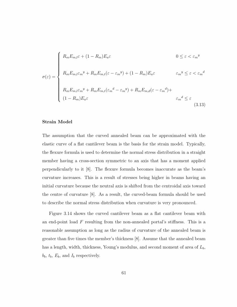
σ(ε) =
RmEm,lε + (1−Rm)Eaε 0 ≤ ε < εmy
RmEm,lεmy + RmEm,t(ε− εm
y) + (1−Rm)Eaε εmy ≤ ε < εm
d
RmEm,lεmy + RmEm,t(εm
d − εmy) + RmEm,d(ε− εm
d)+
(1−Rm)Eaε εmd ≤ ε
(3.13)
Strain Model
The assumption that the curved annealed beam can be approximated with the
elastic curve of a flat cantilever beam is the basis for the strain model. Typically,
the flexure formula is used to determine the normal stress distribution in a straight
member having a cross-section symmetric to an axis that has a moment applied
perpendicularly to it [8]. The flexure formula becomes inaccurate as the beam’s
curvature increases. This is a result of stresses being higher in beams having an
initial curvature because the neutral axis is shifted from the centroidal axis toward
the centre of curvature [8]. As a result, the curved-beam formula should be used
to describe the normal stress distribution when curvature is very pronounced.
Figure 3.14 shows the curved cantilever beam as a flat cantilever beam with
an end-point load F resulting from the non-annealed portal’s stiffness. This is a
reasonable assumption as long as the radius of curvature of the annealed beam is
greater than five times the member’s thickness [8]. Assume that the annealed beam
has a length, width, thickness, Young’s modulus, and second moment of area of Lb,
bb, tb, Eb, and Ib respectively.
61
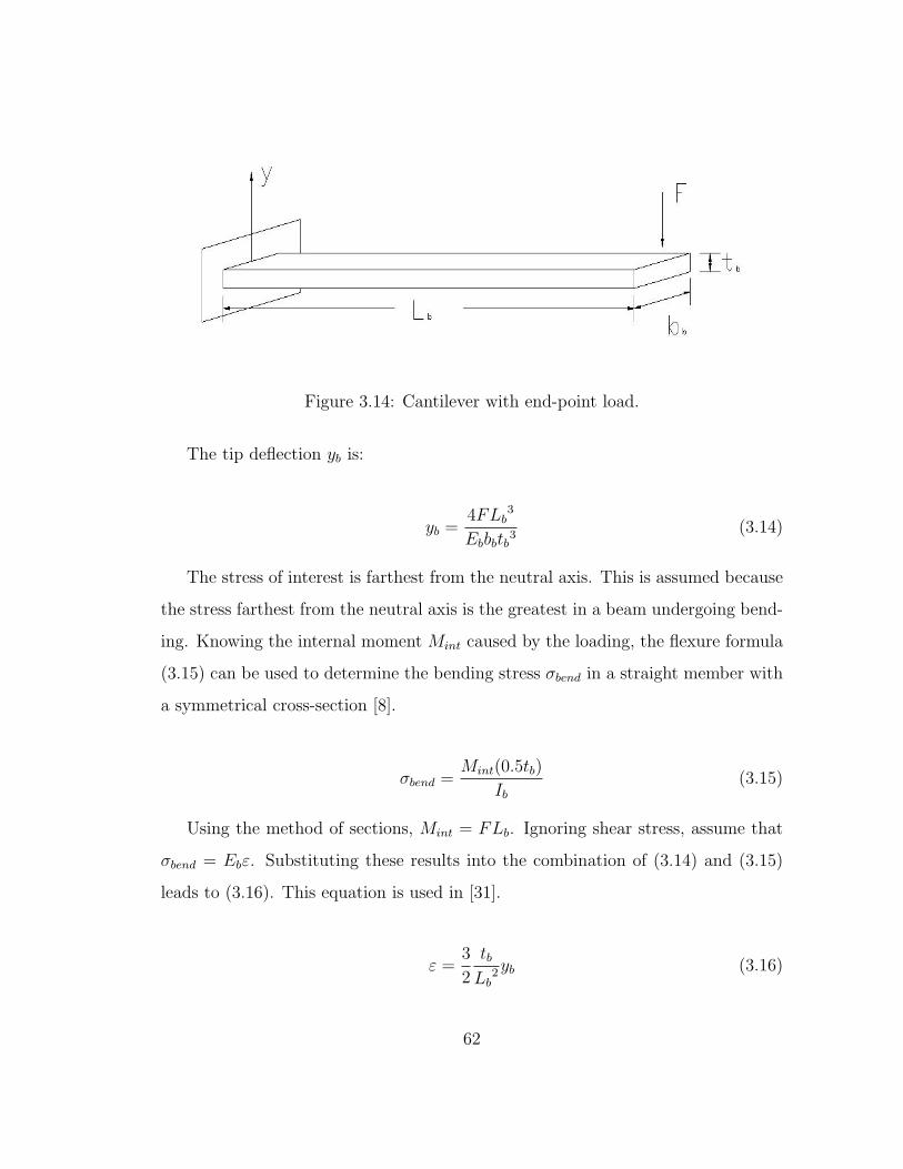
Figure 3.14: Cantilever with end-point load.
The tip deflection yb is:
yb =4FLb
3
Ebbbtb3
(3.14)
The stress of interest is farthest from the neutral axis. This is assumed because
the stress farthest from the neutral axis is the greatest in a beam undergoing bend-
ing. Knowing the internal moment Mint caused by the loading, the flexure formula
(3.15) can be used to determine the bending stress σbend in a straight member with
a symmetrical cross-section [8].
σbend =Mint(0.5tb)
Ib
(3.15)
Using the method of sections, Mint = FLb. Ignoring shear stress, assume that
σbend = Ebε. Substituting these results into the combination of (3.14) and (3.15)
leads to (3.16). This equation is used in [31].
ε =3
2
tb
Lb2yb (3.16)
62

Stress and Strain Model Summary
Figure 3.15 summarizes the non-linear procedure used to obtain Eb given Rm and
yb.
yb
σ
(3.13) (3.8)
(3.16)
ε
Rm Eb
Figure 3.15: Block diagram of stress and strain model.
3.4.4 Phase Model
The non-linear Young’s modulus system model links Rm with T in the phase model.
As the temperature changes, the percentages of crystalline phases vary in the ma-
terial. Ra and Rm are the fraction of austenite and martensite in the material
respectively.
When relating phase fraction and temperature, it is prudent to model the asso-
ciated hysteretic behaviour, including the presence of major and minor hysteresis
loops, and to take the loading conditions into account. The following work is de-
veloped using [18] and [40].
63
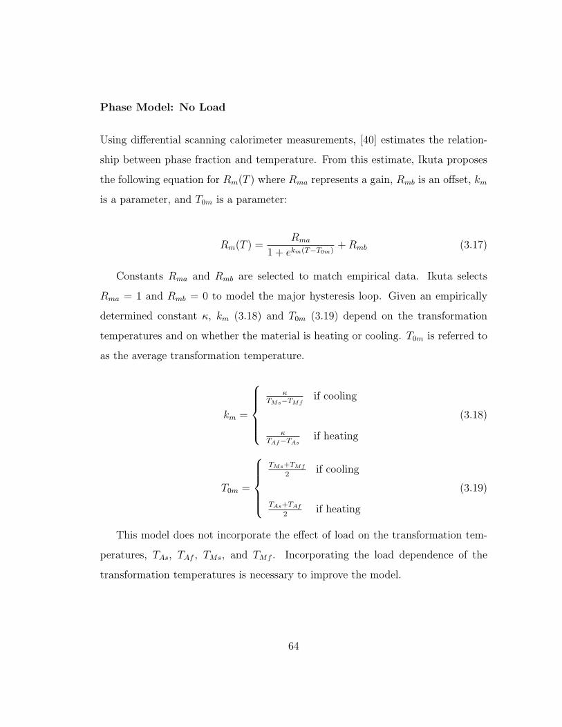
Phase Model: No Load
Using differential scanning calorimeter measurements, [40] estimates the relation-
ship between phase fraction and temperature. From this estimate, Ikuta proposes
the following equation for Rm(T ) where Rma represents a gain, Rmb is an offset, km
is a parameter, and T0m is a parameter:
Rm(T ) =Rma
1 + ekm(T−T0m)+ Rmb (3.17)
Constants Rma and Rmb are selected to match empirical data. Ikuta selects
Rma = 1 and Rmb = 0 to model the major hysteresis loop. Given an empirically
determined constant κ, km (3.18) and T0m (3.19) depend on the transformation
temperatures and on whether the material is heating or cooling. T0m is referred to
as the average transformation temperature.
km =
κ
TMs−TMfif cooling
κTAf−TAs
if heating
(3.18)
T0m =
TMs+TMf
2if cooling
TAs+TAf
2if heating
(3.19)
This model does not incorporate the effect of load on the transformation tem-
peratures, TAs, TAf , TMs, and TMf . Incorporating the load dependence of the
transformation temperatures is necessary to improve the model.
64
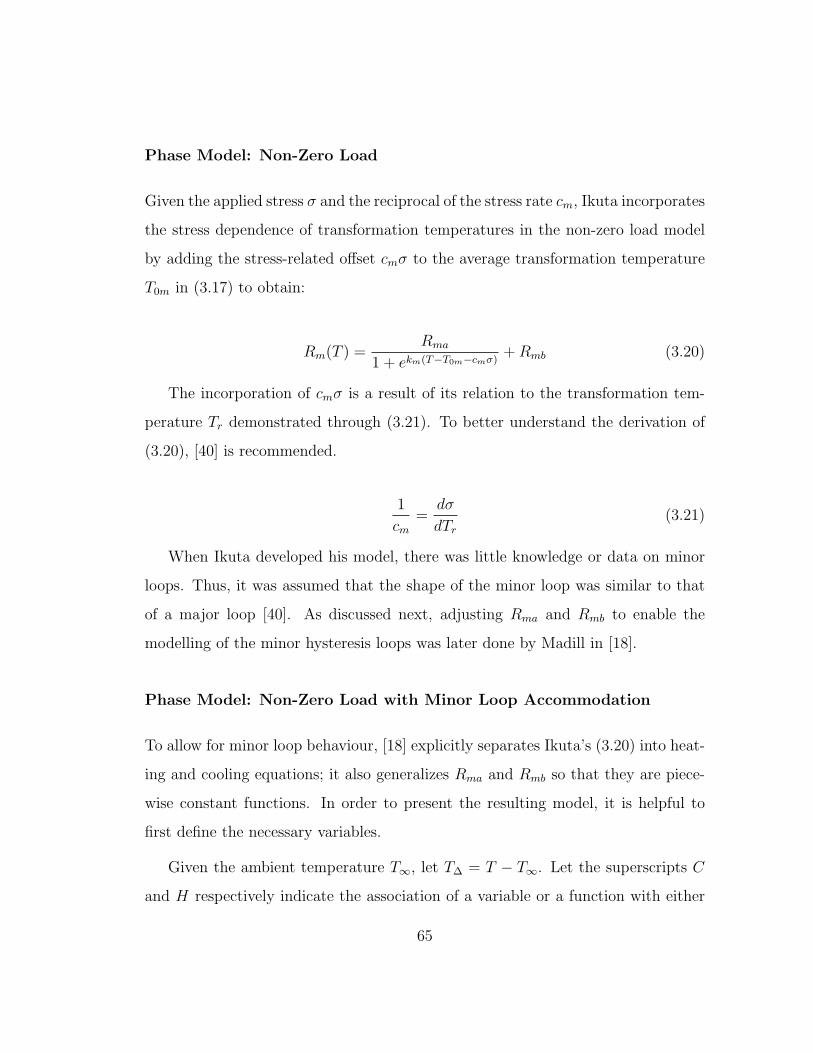
Phase Model: Non-Zero Load
Given the applied stress σ and the reciprocal of the stress rate cm, Ikuta incorporates
the stress dependence of transformation temperatures in the non-zero load model
by adding the stress-related offset cmσ to the average transformation temperature
T0m in (3.17) to obtain:
Rm(T ) =Rma
1 + ekm(T−T0m−cmσ)+ Rmb (3.20)
The incorporation of cmσ is a result of its relation to the transformation tem-
perature Tr demonstrated through (3.21). To better understand the derivation of
(3.20), [40] is recommended.
1
cm
=dσ
dTr
(3.21)
When Ikuta developed his model, there was little knowledge or data on minor
loops. Thus, it was assumed that the shape of the minor loop was similar to that
of a major loop [40]. As discussed next, adjusting Rma and Rmb to enable the
modelling of the minor hysteresis loops was later done by Madill in [18].
Phase Model: Non-Zero Load with Minor Loop Accommodation
To allow for minor loop behaviour, [18] explicitly separates Ikuta’s (3.20) into heat-
ing and cooling equations; it also generalizes Rma and Rmb so that they are piece-
wise constant functions. In order to present the resulting model, it is helpful to
first define the necessary variables.
Given the ambient temperature T∞, let T∆ = T − T∞. Let the superscripts C
and H respectively indicate the association of a variable or a function with either
65
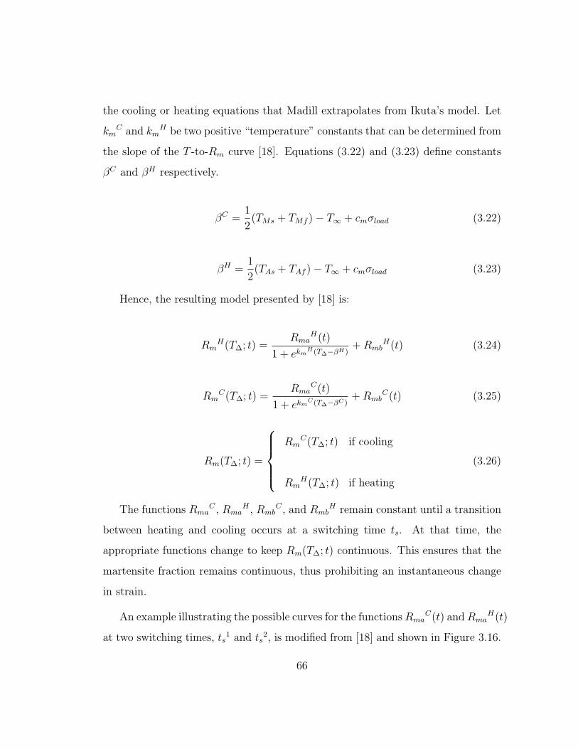
the cooling or heating equations that Madill extrapolates from Ikuta’s model. Let
kmC and km
H be two positive “temperature” constants that can be determined from
the slope of the T -to-Rm curve [18]. Equations (3.22) and (3.23) define constants
βC and βH respectively.
βC =1
2(TMs + TMf )− T∞ + cmσload (3.22)
βH =1
2(TAs + TAf )− T∞ + cmσload (3.23)
Hence, the resulting model presented by [18] is:
RmH(T∆; t) =
RmaH(t)
1 + ekmH(T∆−βH)
+ RmbH(t) (3.24)
RmC(T∆; t) =
RmaC(t)
1 + ekmC(T∆−βC)
+ RmbC(t) (3.25)
Rm(T∆; t) =
Rm
C(T∆; t) if cooling
RmH(T∆; t) if heating
(3.26)
The functions RmaC , Rma
H , RmbC , and Rmb
H remain constant until a transition
between heating and cooling occurs at a switching time ts. At that time, the
appropriate functions change to keep Rm(T∆; t) continuous. This ensures that the
martensite fraction remains continuous, thus prohibiting an instantaneous change
in strain.
An example illustrating the possible curves for the functions RmaC(t) and Rma
H(t)
at two switching times, ts1 and ts
2, is modified from [18] and shown in Figure 3.16.
66
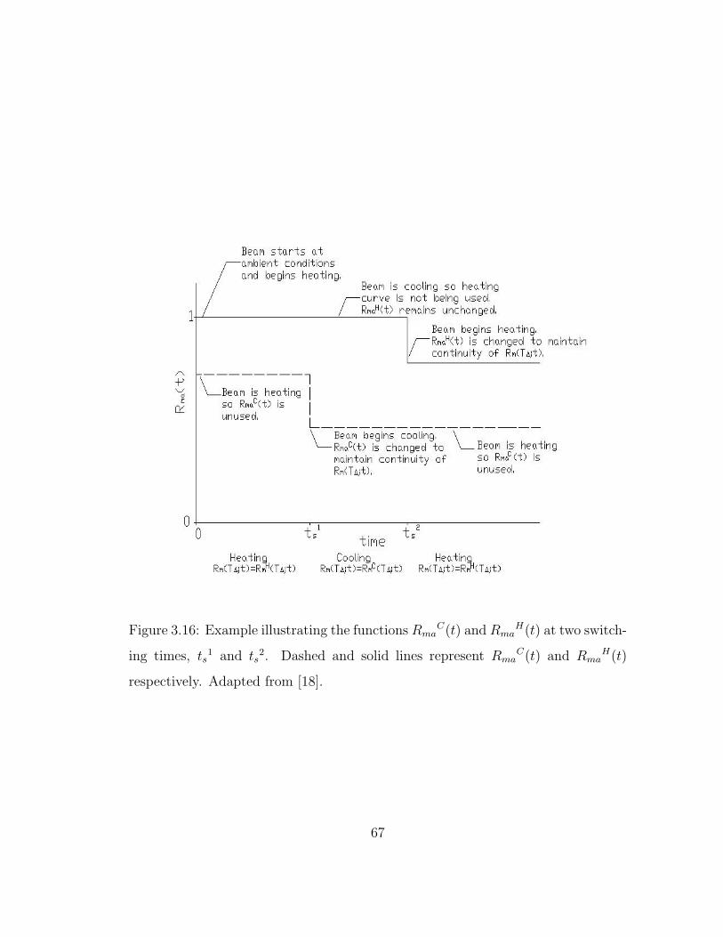
Figure 3.16: Example illustrating the functions RmaC(t) and Rma
H(t) at two switch-
ing times, ts1 and ts
2. Dashed and solid lines represent RmaC(t) and Rma
H(t)
respectively. Adapted from [18].
67
Initial Conditions
The following initial conditions assume that the beam is either fully austenite or
martensite so that its temperature-to-strain relationship begins on the major hys-
teresis curve [18]. Specifying the initial conditions requires non-negative constants
Rma0 and Rmb0 that respectively enable RmC(T∆; 0) and Rm
H(T∆; 0) to describe the
major hysteresis loop. As an approximation, let Rma0 + Rmb0 = 1 and Rmb0 = 0.
These values can be modified to better match empirical data, but they are a good
starting point. RmaC(t = 0), Rmb
C(t = 0), RmaH(t = 0), and Rmb
H(t = 0) are
specified in (3.27), (3.28), (3.29), and (3.30) respectively.
RmaC(t = 0) = Rma0[1 + e−km
CβC
] (3.27)
RmbC(t = 0) = Rmb0 (3.28)
RmaH(t = 0) = Rma0[1 + e−km
HβH
] (3.29)
RmbH(t = 0) = Rmb0 (3.30)
These initial conditions are not unique, but they do satisfy the initial condition
of the annealed beam being initially martensite.
Since the annealed beam begins as martensite, its corresponding strain εm (3.31)
is a function of tb, Lb, and yb,l.
εm(t = 0) =3
2
tb
Lb2yb,l (3.31)
Depending on the value of εm, the appropriate equation from (3.13) can be used
to determine the beam’s initial stress.
68

Switching Conditions: Heating to Cooling
From [18], (3.32) and (3.33) are used in (3.26) to compute Rm if the material
switches from heating to cooling. The equations were derived to ensure continuity
at the switching time ts meaning RmC(T∆, ts) = Rm
H(T∆, ts).
RmaC(ts) = [Rma0 + Rmb0 −Rm
H(Ts; ts)](1 + e−km
CβC)(1 + ekm
C(Ts−βC))
ekmC(Ts−βC) − e−kC
mβC(3.32)
RmbC(ts) = Rma0 + Rmb0 −
RmaC(ts)
1 + e−kmCβC
(3.33)
Switching Conditions: Cooling to Heating
From [18], (3.34) and (3.35) are used in (3.26) to compute Rm if the material
switches from cooling to heating. The equations were derived to ensure continuity
at the switching time ts.
RmaH(ts) = [Rm
C(Ts; ts)−Rmb0](1 + ekmH(Ts−βH
) (3.34)
RmbH(ts) = Rmb0 (3.35)
Madill’s model was derived for an SMA under a constant load. This work
builds from Madill’s model by taking his temperature-to-phase relationships and
incorporating a changing load. Hence at each time interval, the load calculated
at the previous time step using the stress and strain model is incorporated into
Madill’s work to compute the new phase fraction.
69
3.4.5 Heating Model
As mentioned above, the input current I directly affects the annealed beam’s tem-
perature T . Applying the first law of thermodynamics leads to a heating model.
This requires the identification of energy terms. The terms Ein and Eout relate
to the thermal and mechanical energy entering and leaving through a differential
control surface respectively. Egen specifies the generation of energy; energy stored
in the control volume is Est. The first law of thermodynamics requires conservation
of energy. The rate equation (3.36) expresses this conservation.
dEst
dt=
dEin
dt− dEout
dt+
dEgen
dt(3.36)
Conservation of energy requires that the change in the beam’s internal heat en-
ergy equals the energy generated from electric resistance heating minus the energy
lost due to convection and radiation. Convective heat transfer occurs between a
fluid in motion and a surface when the two are at different temperatures [7]. The
nature of the flow characterizes whether the convection is forced, free, or a mixture
of the two. Forced convection occurs when the flow is caused by an external means
whereas free convection occurs due to buoyancy forces that arise from density dif-
ferences caused by temperature variations in the fluid. Radiation is the mode of
heat transfer that occurs since all surfaces of finite temperature emit energy in the
form of electromagnetic waves. In the absence of an intervening medium, there is
net heat transfer by radiation between two surfaces at different temperatures [7].
Conduction refers to the heat transfer that occurs across the medium [7]. It is as-
sumed that the temperature is constant throughout the actuator because the beam
is relatively short and thin. Since there is no spatial thermal distribution, there is
no conductive energy flow. The beam’s specific heat csh, volume Vb, surface area Ab,
70

resistivity ρe, and density ρm are assumed to be independent of temperature. The
temperature of the surroundings is T∞. Assuming Pe is the electrical input power
and htc is the convection heat transfer coefficient, the energy equation becomes:
ρmcshVbdT
dt= Pe − htcAb(T − T∞) (3.37)
Note that (3.37) ignores the effects of radiation and temperature gradients
within the actuator. Ignoring the effects of radiation is possible given that 25C ≤
TMf ≤ T ≤ TAf ≤ 60C. In this temperature range, heat transfer by radiation is
much less than heat transfer by convection. Though the middle beam will heat at
its mid-length first, the temperature gradients within the material are ignored since
the time required for the system to reach steady-state within the relatively short,
thin beam is deemed not significant for this first approximation.
Taking the Laplace transform of (3.37) and assuming that the beam is initially
at T∞ leads to:
T (s) =
ρe
ρmcshb2bt2b
s + htc2(bb+tb)ρmcshbbtb
I2 + T∞ (3.38)
This equation was developed using [7] and [18].
3.5 Equivalent Mass of Annealed Beam
This section focuses on the development of the annealed beam’s equivalent mass
mb. The equivalent mass of the annealed beam can be obtained by determining the
system’s kinetic energy. For the annealed beam, the kinetic energy Kb,bend results
from the cantilever deflection caused by bending.
71
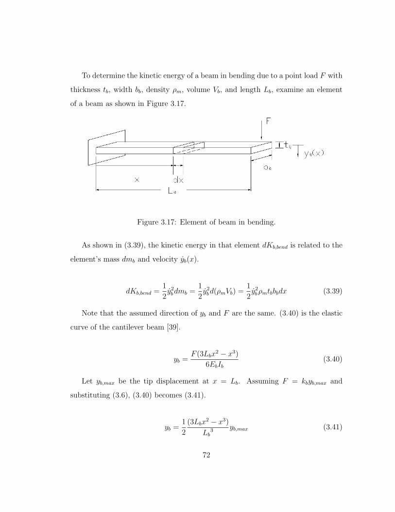
To determine the kinetic energy of a beam in bending due to a point load F with
thickness tb, width bb, density ρm, volume Vb, and length Lb, examine an element
of a beam as shown in Figure 3.17.
Figure 3.17: Element of beam in bending.
As shown in (3.39), the kinetic energy in that element dKb,bend is related to the
element’s mass dmb and velocity yb(x).
dKb,bend =1
2y2
bdmb =1
2y2
bd(ρmVb) =1
2y2
bρmtbbbdx (3.39)
Note that the assumed direction of yb and F are the same. (3.40) is the elastic
curve of the cantilever beam [39].
yb =F (3Lbx
2 − x3)
6EbIb
(3.40)
Let yb,max be the tip displacement at x = Lb. Assuming F = kbyb,max and
substituting (3.6), (3.40) becomes (3.41).
yb =1
2
(3Lbx2 − x3)
Lb3 yb,max (3.41)
72
Taking the derivative of (3.41) with respect to time leads to (3.42).
yb =1
2
(3Lbx2 − x3)
Lb3 yb,max (3.42)
Summing the kinetic energy of all the beam elements and substituting (3.42)
results in (3.43).
Kb,bend =
∫ Lb
0
1
2y2
bρmtbbbdx =33
280y2
b,maxρmtbbbLb (3.43)
Given the equivalent lumped mass of the annealed beam mb, the annealed
beam’s maximum kinetic energy Kb,max is (3.44).
Kb,max =1
2mby
2b,max (3.44)
The summation of the kinetic energy in the system equals the maximum kinetic
energy. Thus, equating (3.43) with (3.44) and solving for mb leads to (3.45).
mb =33
140ρmbbtbLb (3.45)
3.6 Equivalent Stiffness of Non-Annealed Portal
The purpose of this section is to obtain an expression for the equivalent stiffness of
the non-annealed portal. Non-annealed NiTi will not display the SME. Hence, any
current flowing in the portal will not affect its equivalent stiffness. To develop this
section, [8] and [39] were used.
Consider the non-annealed portal seen in Figure 3.18. LAB and LBC correspond
to the lengths of sections AB and BC respectively. Note that cantilevers AB and
73

DC have equal lengths. The widths and thicknesses of sections AB and DC are
the same, and they are represented by bAB and tAB respectively. The width and
thickness of section BC are bBC and tBC respectively. Note that sections AB, DC,
and BC have equal thicknesses. The portal has a Young’s modulus of Ep. When
heated the annealed beam exerts a load on the portal. It is assumed that this load
is strictly in the y-direction. As shown in Figure 3.18, the frame experiences an
out-of-plane load F applied mid-girder.
Figure 3.18: Non-annealed portal.
The portal is a statically indeterminate structure since the number of unknown
reactions exceeds the available number of equilibrium equations [8]. Indeterminate
structures can be solved using the principle of superposition. The principle of super-
position requires that the load be linearly related to the deflection and that the load
not significantly change the original geometry of the beam [8]. Assuming that the
principle of superposition holds, the statically indeterminate structure is equated to
a sequence of statically determinate beams. It is possible to detach cantilevers AB
and DC with the girder BC by ensuring that at their appropriate intersections the
cantilevers and girder have the same values for slope and deflection since the portal
is physically continuous. Hence, the non-annealed portal comprises cantilever AB,
74

cantilever DC, and girder BC. Figure 3.19 shows the free-body diagram of the
portal.
Figure 3.19: Portal free-body diagram.
When using superposition, the deflections for a series of separate loadings acting
on a beam may be superimposed [8]. To determine the moment M shown in Figure
3.19, the effect of each force and moment on the girder is examined separately. Using
superposition, the sum of each resulting deflection determines the total deflection
of the girder. Let y′ be an axis in the same direction as axis y, but let y′ have
its origin at the deflected tip of cantilever AB. The sum of the displacements at
z = LBC must correspond with y′ = 0 since symmetry ensures that z = 0 and
z = LBC have the same deflection at y′. The free-body diagrams for the separate
beams and their loadings are illustrated in Figure 3.20.
Assuming IBC is the second moment of area of the rectangular cross-section
girder, (3.46) is obtained by summing the deflections of the three component parts
at the tip and equating them to zero.
yF/2 + yF + yM =−(F
2)LBC
3
3EpIBC
+5FLBC
3
48EpIBC
+MLBC
2
2EpIBC
= 0 (3.46)
Solving (3.46) for M leads to (3.47).
75
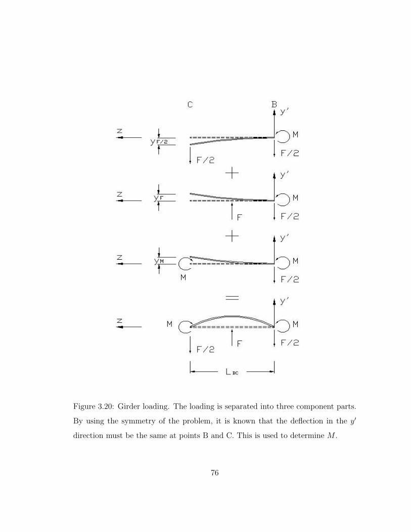
Figure 3.20: Girder loading. The loading is separated into three component parts.
By using the symmetry of the problem, it is known that the deflection in the y′
direction must be the same at points B and C. This is used to determine M .
76
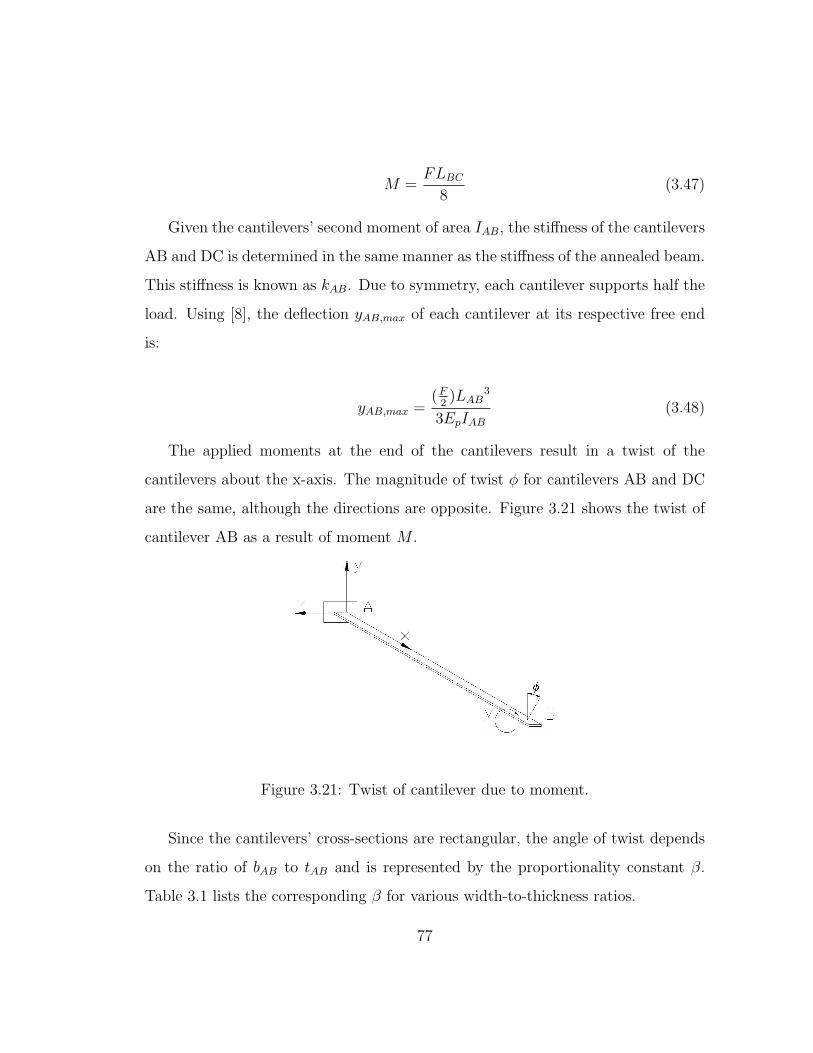
M =FLBC
8(3.47)
Given the cantilevers’ second moment of area IAB, the stiffness of the cantilevers
AB and DC is determined in the same manner as the stiffness of the annealed beam.
This stiffness is known as kAB. Due to symmetry, each cantilever supports half the
load. Using [8], the deflection yAB,max of each cantilever at its respective free end
is:
yAB,max =(F
2)LAB
3
3EpIAB
(3.48)
The applied moments at the end of the cantilevers result in a twist of the
cantilevers about the x-axis. The magnitude of twist φ for cantilevers AB and DC
are the same, although the directions are opposite. Figure 3.21 shows the twist of
cantilever AB as a result of moment M .
Figure 3.21: Twist of cantilever due to moment.
Since the cantilevers’ cross-sections are rectangular, the angle of twist depends
on the ratio of bAB to tAB and is represented by the proportionality constant β.
Table 3.1 lists the corresponding β for various width-to-thickness ratios.
77
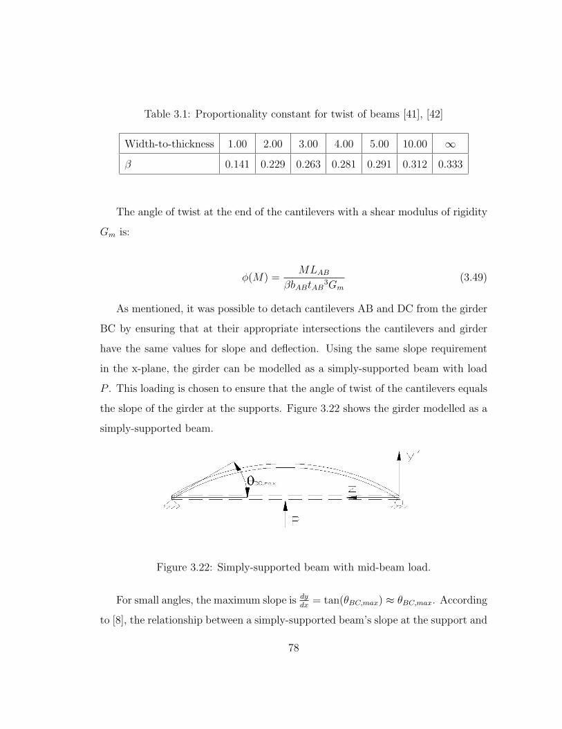
Table 3.1: Proportionality constant for twist of beams [41], [42]
Width-to-thickness 1.00 2.00 3.00 4.00 5.00 10.00 ∞
β 0.141 0.229 0.263 0.281 0.291 0.312 0.333
The angle of twist at the end of the cantilevers with a shear modulus of rigidity
Gm is:
φ(M) =MLAB
βbABtAB3Gm
(3.49)
As mentioned, it was possible to detach cantilevers AB and DC from the girder
BC by ensuring that at their appropriate intersections the cantilevers and girder
have the same values for slope and deflection. Using the same slope requirement
in the x-plane, the girder can be modelled as a simply-supported beam with load
P . This loading is chosen to ensure that the angle of twist of the cantilevers equals
the slope of the girder at the supports. Figure 3.22 shows the girder modelled as a
simply-supported beam.
Figure 3.22: Simply-supported beam with mid-beam load.
For small angles, the maximum slope is dydx
= tan(θBC,max) ≈ θBC,max. According
to [8], the relationship between a simply-supported beam’s slope at the support and
78
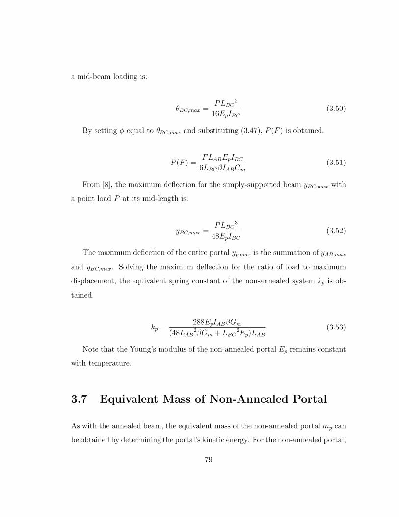
a mid-beam loading is:
θBC,max =PLBC
2
16EpIBC
(3.50)
By setting φ equal to θBC,max and substituting (3.47), P (F ) is obtained.
P (F ) =FLABEpIBC
6LBCβIABGm
(3.51)
From [8], the maximum deflection for the simply-supported beam yBC,max with
a point load P at its mid-length is:
yBC,max =PLBC
3
48EpIBC
(3.52)
The maximum deflection of the entire portal yp,max is the summation of yAB,max
and yBC,max. Solving the maximum deflection for the ratio of load to maximum
displacement, the equivalent spring constant of the non-annealed system kp is ob-
tained.
kp =288EpIABβGm
(48LAB2βGm + LBC
2Ep)LAB
(3.53)
Note that the Young’s modulus of the non-annealed portal Ep remains constant
with temperature.
3.7 Equivalent Mass of Non-Annealed Portal
As with the annealed beam, the equivalent mass of the non-annealed portal mp can
be obtained by determining the portal’s kinetic energy. For the non-annealed portal,
79

the kinetic energy is a summation of the system’s kinetic energy due to cantilever
deflection caused by bending in cantilevers AB and DC, cantilever twisting due to
torsion in cantilevers AB and DC, and girder deflection caused by bending in girder
BC. These are known as Kp,c,bend, Kp,c,rot, and Kp,g,bend respectively. The portal has
density ρm and its maximum velocity, which occurs at the girder centre, is yp,max.
The same procedure used to determine Kb,bend is also used to determine the
kinetic energy in the non-annealed cantilever beams due to deflection changes re-
sulting from the end-point load F2. The result is:
Kp,c,bend =11
3360
ρmtABbABkp2y2
p,maxLAB7
Ep2IAB
2 (3.54)
Given the twist of the portal’s cantilever beams φ, the moment of inertia about
the axis of rotation Ix, the mass of each cantilever mcant, and the angular velocity
ω, the kinetic energy due to torsion in a cantilever element dKp,c,rot is:
dKp,c,rot =1
2dIxω
2 (3.55)
The moment of inertia about the axis of rotation Ix and the angle of twist in a
rectangular cantilever beam φ are given by (3.56) and (3.57) respectively [41].
dIx =mcant
12(tAB
2 + bAB2) =
ρmtABbABdx
12(tAB
2 + bAB2) (3.56)
φ =Mx
βbABtAB3Gm
(3.57)
The time derivative of the angle of twist φ is equal to ω. After substituting
F = kpyp,max, (3.47), (3.56), and (3.57) into (3.55), and summing all elements, the
kinetic energy due to torsion is:
80
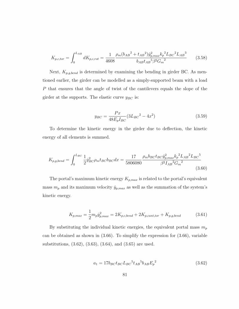
Kp,c,tor =
∫ LAB
0
dKp,c,rot =1
4608
ρm(bAB2 + tAB
2)y2p,maxkp
2LBC2LAB
3
bABtAB5β2Gm
2 (3.58)
Next, Kp,g,bend is determined by examining the bending in girder BC. As men-
tioned earlier, the girder can be modelled as a simply-supported beam with a load
P that ensures that the angle of twist of the cantilevers equals the slope of the
girder at the supports. The elastic curve yBC is:
yBC =Px
48EpIBC
(3LBC2 − 4x2) (3.59)
To determine the kinetic energy in the girder due to deflection, the kinetic
energy of all elements is summed.
Kp,g,bend =
∫ LBC
0
1
2y2
BCρmtBCbBCdx =17
5806080
ρmbBCtBC y2p,maxkp
2LAB2LBC
5
β2IAB2Gm
2
(3.60)
The portal’s maximum kinetic energy Kp,max is related to the portal’s equivalent
mass mp and its maximum velocity yp,max as well as the summation of the system’s
kinetic energy.
Kp,max =1
2mpy
2p,max = 2Kp,c,bend + 2Kp,cant,tor + Kp,g,bend (3.61)
By substituting the individual kinetic energies, the equivalent portal mass mp
can be obtained as shown in (3.66). To simplify the expression for (3.66), variable
substitutions, (3.62), (3.63), (3.64), and (3.65) are used.
a1 = 17bBCtBCLBC5tAB
5bABEp2 (3.62)
81
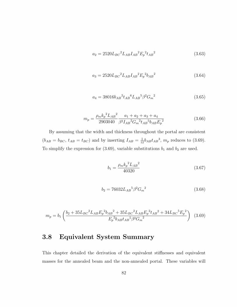
a2 = 2520LBC2LABIAB
2Ep2tAB
2 (3.63)
a3 = 2520LBC2LABIAB
2Ep2bAB
2 (3.64)
a4 = 38016bAB2tAB
6LAB5β2Gm
2 (3.65)
mp =ρmkp
2LAB2
2903040
a1 + a2 + a3 + a4
β2IAB2Gm
2tAB5bABEp
2 (3.66)
By assuming that the width and thickness throughout the portal are consistent
(bAB = bBC , tAB = tBC) and by inserting IAB = 112
bABtAB3, mp reduces to (3.69).
To simplify the expression for (3.69), variable substitutions b1 and b2 are used.
b1 =ρmkp
2LAB2
40320(3.67)
b2 = 76032LAB5β2Gm
2 (3.68)
mp = b1
(b2 + 35LBC
2LABEp2bAB
2 + 35LBC2LABEp
2tAB2 + 34LBC
5Ep2
Ep2bABtAB
5β2Gm2
)(3.69)
3.8 Equivalent System Summary
This chapter detailed the derivation of the equivalent stiffnesses and equivalent
masses for the annealed beam and the non-annealed portal. These variables will
82

be used in the equivalent lumped model for design and simulation of the actua-
tor. The variables in conjunction with the lumped model provide understanding
of the proposed actuator’s behaviour. The next chapter outlines the dimensional
specifications of the actuator.
83
Chapter 4
Dimension Selection and
Parameters
SMAs provide exciting opportunities for miniature robots. As previously men-
tioned, this material can be used to create lightweight, powerful actuators that
can be scaled down if designed to be mechanically simple. The mechanically sim-
ple monolithic design introduced in the previous chapter has good potential to be
scaled to a specific size. This chapter selects dimensions for a centimetre-scale
monolithic SMA actuator and lists the material properties required for simulation.
After proof-of-concept, it will be possible to shrink the actuator to dimensions that
satisfy the constraints of the intended environment.
Since comparison of simulated and experimental results permit model validation,
the dimensions and properties of the actuator used in simulations must match those
of the prototype. The prototype is constructed using a 6.99mm-wide, 0.25mm-
thick NiTi SM495 strip from Nitinol Devices & Components. The length of the
girder LBC is equal to the sample width. The beam width bb and the portal’s
84
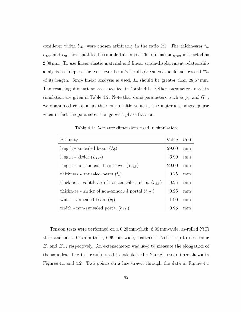
cantilever width bAB were chosen arbitrarily in the ratio 2:1. The thicknesses tb,
tAB, and tBC are equal to the sample thickness. The dimension yflat is selected as
2.00mm. To use linear elastic material and linear strain-displacement relationship
analysis techniques, the cantilever beam’s tip displacement should not exceed 7%
of its length. Since linear analysis is used, Lb should be greater than 28.57mm.
The resulting dimensions are specified in Table 4.1. Other parameters used in
simulation are given in Table 4.2. Note that some parameters, such as ρe, and Gm,
were assumed constant at their martensitic value as the material changed phase
when in fact the parameter change with phase fraction.
Table 4.1: Actuator dimensions used in simulation
Property Value Unit
length - annealed beam (Lb) 29.00 mm
length - girder (LBC) 6.99 mm
length - non-annealed cantilever (LAB) 29.00 mm
thickness - annealed beam (tb) 0.25 mm
thickness - cantilever of non-annealed portal (tAB) 0.25 mm
thickness - girder of non-annealed portal (tBC) 0.25 mm
width - annealed beam (bb) 1.90 mm
width - non-annealed portal (bAB) 0.95 mm
Tension tests were performed on a 0.25mm-thick, 6.99mm-wide, as-rolled NiTi
strip and on a 0.25mm-thick, 6.99mm-wide, martensite NiTi strip to determine
Ep and Em,l respectively. An extensometer was used to measure the elongation of
the samples. The test results used to calculate the Young’s moduli are shown in
Figures 4.1 and 4.2. Two points on a line drawn through the data in Figure 4.1
85
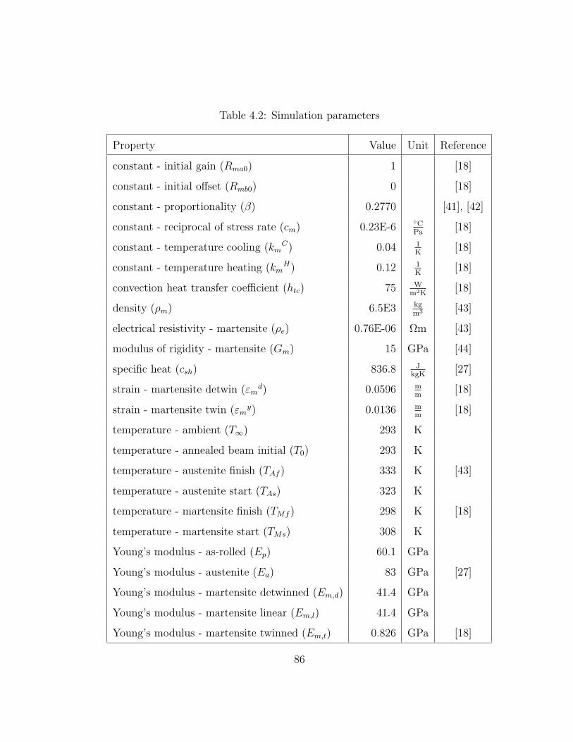
Table 4.2: Simulation parameters
Property Value Unit Reference
constant - initial gain (Rma0) 1 [18]
constant - initial offset (Rmb0) 0 [18]
constant - proportionality (β) 0.2770 [41], [42]
constant - reciprocal of stress rate (cm) 0.23E-6CPa
[18]
constant - temperature cooling (kmC) 0.04 1
K[18]
constant - temperature heating (kmH) 0.12 1
K[18]
convection heat transfer coefficient (htc) 75 Wm2K
[18]
density (ρm) 6.5E3 kgm3 [43]
electrical resistivity - martensite (ρe) 0.76E-06 Ωm [43]
modulus of rigidity - martensite (Gm) 15 GPa [44]
specific heat (csh) 836.8 JkgK
[27]
strain - martensite detwin (εmd) 0.0596 m
m[18]
strain - martensite twin (εmy) 0.0136 m
m[18]
temperature - ambient (T∞) 293 K
temperature - annealed beam initial (T0) 293 K
temperature - austenite finish (TAf ) 333 K [43]
temperature - austenite start (TAs) 323 K
temperature - martensite finish (TMf ) 298 K [18]
temperature - martensite start (TMs) 308 K
Young’s modulus - as-rolled (Ep) 60.1 GPa
Young’s modulus - austenite (Ea) 83 GPa [27]
Young’s modulus - martensite detwinned (Em,d) 41.4 GPa
Young’s modulus - martensite linear (Em,l) 41.4 GPa
Young’s modulus - martensite twinned (Em,t) 0.826 GPa [18]
86

were used to determine the slope of the as-rolled NiTi sample. To determine the
slope of the martensite NiTi sample, two points on a line drawn through points
corresponding to strains of 0.001 mm
and 0.0005 mm
were used. Em,d is assumed to be
equal to Em,l.
0.00E+00
2.00E+07
4.00E+07
6.00E+07
8.00E+07
1.00E+08
1.20E+08
1.40E+08
1.60E+08
0.0000 0.0005 0.0010 0.0015 0.0020 0.0025
strain (m/m)
stre
ss (
Pa)
Figure 4.1: Tension test using as-rolled NiTi sample.
The dimensions of the prototype are shown in Figure 4.3. The holes shown are
used to position the prototype in a heating fixture to impart the high-temperature
shape on the middle beam. Using 4-40 screws for the alignment holes led to an
actuator length of 45.00mm. Respecting the assumption constraints and the NiTi
87

0.00E+00
2.00E+07
4.00E+07
6.00E+07
8.00E+07
1.00E+08
1.20E+08
1.40E+08
0.0000 0.0005 0.0010 0.0015 0.0020 0.0025 0.0030 0.0035
strain (m/m)
stre
ss (
Pa)
Figure 4.2: Tension test using martensite NiTi sample.
88

strip dimensions led to the dimensions shown in Figure 4.3. All dimensions are in
millimetres.
Figure 4.3: Monolithic prototype actuator dimensions. All dimensions are in mil-
limetres.
Using yflat = 2.00mm and the modelling equations developed in Chapter 3,
deflections, strains, equivalent masses, and equivalent stiffnesses were calculated.
They are listed in Table 4.3.
As shown in Table 4.3, the computed strain values, εa and εm, do not exceed
εmy. This indicates that the middle beam does not detwin while martensite. Recall
the equation for ε:
ε =3
2
tb
Lb2yb (4.1)
A design choice set the middle beam’s tip displacement to 7% of its length.
Substituting this constraint on yb and replacing ε with εmy in (4.1) leads to:
εmy =
3
2
tb
Lb2
7
100Lb (4.2)
89

Table 4.3: Model parameter calculations
Property Value Unit Equation
deflection - annealed beam at TAf (yb,h) 0.83 mm (3.3)
deflection - annealed beam at TMf (yb,l) 1.18 mm (3.2)
deflection - annealed beam total tip (ytip) 0.34 mm
deflection - curved to flat (yflat) 2.00 mm (3.4)
equivalent mass - annealed beam (mb) 2.11E-05 kg (3.45)
equivalent mass - portal (mp) 2.04E-05 kg (3.66)
equivalent stiffness - annealed beam at TAf (kb,h) 25.26 Nm
(3.6)
equivalent stiffness - annealed beam at TMf (kb,l) 12.60 Nm
(3.6)
equivalent stiffness - portal (kp) 17.97 Nm
(3.53)
strain - annealed beam when austenite (εa) 0.037 % (3.16)
strain - annealed beam when martensite (εm) 0.052 % (3.16)
90

The corresponding thickness-to-length relationship of 0.13 dictates whether the
material will detwin. Hence, the middle beam is not able to detwin given the
thickness of the supplied strip and the thickness-to-length requirements of a beam.
After setting the dimensions of the actuator for a specific tip deflection, it is
possible to determine the annealed beam’s radius of curvature. Given Figure 4.4,
the length of the middle beam plus the width of the portal corresponds to the arc
length s of a circle segment with a radius R and angle θ. Note that a corresponds
to the horizontal distance between the start and end of the annealed beam plus the
width of the girder. Variable b corresponds to the difference in tip displacement
from a flat position to where the middle beam is in its high-temperature equilibrium
position. Thus, s = Lb + bp = 29.95 mm and b = yflat = 2.00 mm.
Figure 4.4: Circle segment.
Since R, θ, and a are unknown, it is necessary to relate them using geometry.
This relationship is shown in (4.3).
s = Rθ (4.3)
Using trigonometry and Figure 4.4, (4.4) and (4.5) are obtained.
91
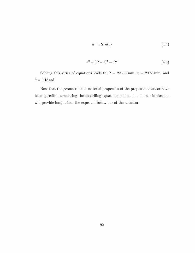
a = Rsin(θ) (4.4)
a2 + (R− b)2 = R2 (4.5)
Solving this series of equations leads to R = 223.92 mm, a = 29.86 mm, and
θ = 0.13 rad.
Now that the geometric and material properties of the proposed actuator have
been specified, simulating the modelling equations is possible. These simulations
will provide insight into the expected behaviour of the actuator.
92

Chapter 5
Analytical Simulations
This chapter uses the dimensions and material properties listed in the previous
chapter to simulate the proposed actuator’s response to an input current. Two
different models - linear Young’s modulus system model [compare Figure 3.5] and
non-linear Young’s modulus system model [compare Figure 3.6] - are simulated and
compared to test the validity of the models and the effect of incorporating various
aspects of the material’s behaviour.
5.1 Linear Young’s Modulus System Model
Using the values from Tables 4.1, 4.2, and 4.3, the dynamic equation (3.1) was
simulated using Simulink r© [45]. Figure 5.1 summarizes the equations used to
obtain yb for this model. Section 5.3 shows the results from simulations using this
model.
93
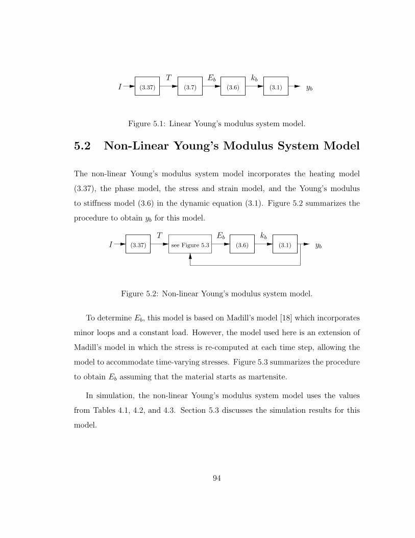
kbEb
I (3.1) yb
T(3.7) (3.6)(3.37)
Figure 5.1: Linear Young’s modulus system model.
5.2 Non-Linear Young’s Modulus System Model
The non-linear Young’s modulus system model incorporates the heating model
(3.37), the phase model, the stress and strain model, and the Young’s modulus
to stiffness model (3.6) in the dynamic equation (3.1). Figure 5.2 summarizes the
procedure to obtain yb for this model.
kbEb
see Figure 5.3 (3.1) yb(3.6)IT
(3.37)
Figure 5.2: Non-linear Young’s modulus system model.
To determine Eb, this model is based on Madill’s model [18] which incorporates
minor loops and a constant load. However, the model used here is an extension of
Madill’s model in which the stress is re-computed at each time step, allowing the
model to accommodate time-varying stresses. Figure 5.3 summarizes the procedure
to obtain Eb assuming that the material starts as martensite.
In simulation, the non-linear Young’s modulus system model uses the values
from Tables 4.1, 4.2, and 4.3. Section 5.3 discusses the simulation results for this
model.
94

Using (3.24) and (3.26),calculate Rm(T∆; t).Using (3.25) and (3.26),
Using (3.32) and (3.33), calculate
Let heat=FALSE.Let heat=TRUE.Rma
H(ts) and RmbH(ts). Rma
C(ts) and RmbC(ts).
Using (3.34) and (3.35), calculate
Is T∆ ≥ T∆P ?Is T∆ ≥ T∆P ?
βH(0), RmaC(0), Rmb
C(0),
Using (3.22), (3.23), (3.27), (3.28),(3.29), and (3.30), calculate βC(0),
Rm = 1, and T∆P = 0.
calculate Rm(T∆; t).
Calculate T∆. Let t = t + ∆t.and (3.23). Set T∆P = T∆.Calculate βC and βH using (3.22)
Calculate ε using (3.16).Calculate σ using (3.13).
Calculate Eb using (3.8).
heat=TRUE?
RmaH(0), and Rmb
H(0).
Is
NO NO
YES YES
NO YES
Let t = 0, T∆ = T − T∞ ≥ 0,
Calculate σ at yb,l using (3.13).Calculate εm using (3.31).
heat=TRUE, Rma0 = 1, Rmb0 = 0,
Figure 5.3: Computing Eb for non-linear model.
95
5.3 Simulation Results
The two models - linear Young’s modulus system model and non-linear Young’s
modulus system model - were simulated using the Runge-Kutta solver. The simu-
lations ran for 20 s with a fixed step size of 0.001 s. A pulse generator was used to
create a current with a 5 s period and a duty cycle of 20%. Input current was com-
puted by using recommended actuation current densities for Flexinol r© [46] and
extrapolating to match the cross-sectional area of the annealed beam. Ambient
temperature was set to T∞ = 293K. Along with the input current, the annealed
beam’s simulated temperature, martensite phase fraction, Young’s modulus, and
tip deflection are shown in Figures 5.4, 5.5, 5.6, and 5.7 respectively. Figure 5.8
shows the martensite phase fracture and the temperature of the annealed beam.
Due to the choice of duty cycle and period for the control current, the actuator
undergoes partial cycling. When the current flows, the temperature of the annealed
beam increases. When the current ceases, the temperature of the annealed beam
decreases. This behaviour is confirmed by the simulation shown in Figure 5.4.
The linear model does not directly calculate Rm. It implicitly assumes that Rm
is linearly related to T , meaning that at T ≤ TMf Rm = 1 and at T ≥ TAf Rm = 0.
Linear interpolation between these extreme temperatures allows for the determina-
tion of Rm for the linear model. In the non-linear model, Rm is computed based on
the procedure outlined in Figure 5.3. As shown in Figure 5.5, the annealed beam is
initially martensite, but its Rm decreases as the annealed beam’s temperature in-
creases due to the resistive heating caused by the input current. When the current
is removed, the material switches from heating to cooling, and Rm increases.
The linear model does not account for the effects of hysteresis or the effects of
minor loops when relating T and Eb. Correspondingly, Figure 5.6 shows that Eb
96

0 5 10 15 20280
300
320
340
360
380
tem
pera
ture
of a
nnea
led
beam
(K)
time (s)0 5 10 15 20
0
2
4
6
8
10
inpu
t cur
rent
(A)
TI
Figure 5.4: Temperature of annealed beam and input current.
97
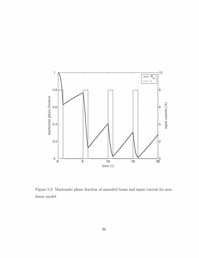
0 5 10 15 200
0.2
0.4
0.6
0.8
1
mar
tens
ite p
hase
frac
tion
time (s)0 5 10 15 20
0
2
4
6
8
10
inpu
t cur
rent
(A)
Rm
I
Figure 5.5: Martensite phase fraction of annealed beam and input current for non-
linear model.
98
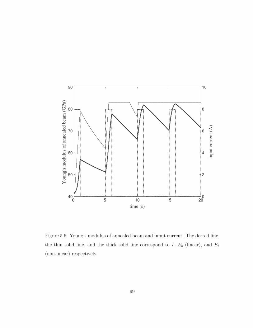
0 5 10 15 2040
50
60
70
80
90
You
ng's
mod
ulus
of a
nnea
led
beam
(GPa
)
time (s)0 5 10 15 20
0
2
4
6
8
10
inpu
t cur
rent
(A)
Figure 5.6: Young’s modulus of annealed beam and input current. The dotted line,
the thin solid line, and the thick solid line correspond to I, Eb (linear), and Eb
(non-linear) respectively.
99
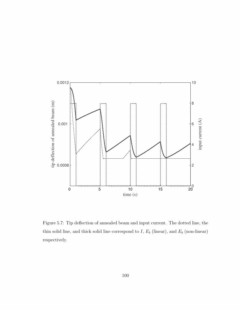
0 5 10 15 20
0.0008
0.001
0.0012
tip d
efle
ctio
n of
ann
eale
d be
am (m
)
time (s)0 5 10 15 20
0
2
4
6
8
10
inpu
t cur
rent
(A)
Figure 5.7: Tip deflection of annealed beam and input current. The dotted line, the
thin solid line, and thick solid line correspond to I, Eb (linear), and Eb (non-linear)
respectively.
100

290 300 310 320 330 340 350 360 3700
0.1
0.2
0.3
0.4
0.5
0.6
0.7
0.8
0.9
1
temperature (K)
mar
tens
ite p
hase
frac
tion
Figure 5.8: Martensite phase fraction and temperature of annealed beam.
101

determined from the linear model is always a line. Figure 5.6 also shows that the Eb
determined from the non-linear model is not linear. This is a result of incorporating
hysteresis and minor loops to obtain a more realistic model.
The behaviour of the annealed beam’s tip is shown in Figure 5.7. Initially, the
annealed beam of the actuator is at the ambient temperature in its martensitic
state, resting at the low-temperature equilibrium tip deflection yb,l. When current
flows through the annealed beam, its temperature increases. Once the annealed
beam reaches TAs, the beam starts to move toward yb,h in the linear model. In
the non-linear model, the beam starts to move toward yb,h as the beam heats, but
the rate at which it moves toward yb,h increases as its temperature approaches
TAs. The current is then turned off for 4 s and the annealed beam’s temperature
decreases causing its stiffness kb(T ) to decrease. With the portal acting as a bias
spring, the tip returns toward yb,l. Before the material can completely cool, more
current is injected and the temperature rises once more. This pattern continues
until eventually yb,h is reached. Note that yb,h is less than yb,l. Note that at low
temperature, the beam is in its martensitic high-strain state whereas the portal is in
its non-annealed low-strain state. At high temperature, the beam is in its austenitic
low-strain state whereas the portal is in its non-annealed high-strain state. Note
that the same ytip is expected from both the linear and non-linear models provided
that the middle beam is fully transformed.
Figure 5.8 demonstrates that the continuity of the martensite phase fraction is
always maintained even though the system switches between heating and cooling.
Continuity is ensured by changing the values of the piece-wise constant functions
RmaC , Rmb
C , RmaH , and Rmb
H each time the system changes from heating to
cooling or from cooling to heating [18].
The period and duty cycle of the control current shown were chosen to demon-
102
strate the incorporation of heating and cooling, and the effectiveness of using
temperature-dependent stiffness in the lumped-parameter end-point displacement
model. This current is not ideal for actual operation, and a higher duty cycle and
longer period would provide consistent, full, open-loop cycling. Though it is in-
tended that the actuator always undergo full cycling, thus eliminating the need for
a precise hysteresis model, improving the model’s handling of minor hysteresis is
certainly helpful in understanding the anticipated behaviour.
These simulations indicate that the annealed beam and non-annealed portal
work together to achieve the desired motion. The next step is to develop a prototype
that verifies this behaviour.
103

Chapter 6
Monolithic Prototype Fabrication
Prototyping is necessary to determine a model’s validity. To ensure the actuator’s
intended functionality, it is critical to machine the actuator geometry from a single
piece of non-annealed NiTi and to locally anneal the middle cantilever beam. There
are various ways to construct a monolithic actuator as discussed in Section 2.3.6.
Local annealing can be achieved by using a laser beam or by directly applying high
current to a material. Another method to locally anneal a device is by using an
indirect heating method, such as a resistive heating element in contact with the
material. Given that a laser beam is inaccessible, the indirect heating method was
deemed the simpler method of the two remaining methods. As a result, using an
indirect heating method was seen as the preferred method to develop a prototype.
Before considering the machining of the actuator, the fixture design, or the anneal-
ing of the actuator, a brief discussion of a proof-of-concept composite prototype
takes place.
This composite prototype comprises a strip of NiTi that displays the SME,
two non-annealed strips of NiTi, and two pieces of aluminium. Though it is not
104

a monolithic device, it was hypothesized that its functionality could illustrate the
proposed actuator’s feasibility. It was meant to be a simple proof-of-concept that
did not require local annealing, but would show that the geometry would work
together as intended.
To obtain the strip of NiTi that displays the SME, a 6.99mm-wide, 62.70mm-
long, 0.25mm-thick NiTi sample was placed between clay dies as shown in Figure 6.1.
The length of the NiTi strip equals the arc length of the mating faces of the clay
fixture after firing. The fixture-sandwiched SMA strip was placed in a 538C kiln
for approximately ten minutes. Once removed, it was quenched in water. Since the
clay dies are not smooth, the SMA strip was bumpy in its high-temperature shape.
Another 62.70mm strip from the same NiTi material was sheared into two ap-
proximately equal-width pieces. To constrain the NiTi strips in the length direction,
two pieces of aluminium were used. Each piece of aluminium was folded in half,
and the strips of NiTi were laid out so that the non-annealed strips were on the
outside and the annealed strip was in the middle. The aluminium was then pressed
to ensure that the NiTi strips would not move. Aluminium strips were used instead
of NiTi strips since the width of the provided NiTi was not sufficient to fold in half
and hold the long NiTi strips. Figure 6.1 shows the composite prototype and the
clay dies used.
When heated, the annealed beam caused the portal to lift. Unfortunately, the
folded piece of aluminium at the beams’ lifting tips was not strong enough to hold
the materials together.
Another concern with the composite model is that the portal’s girder is made
of aluminium. Thus, the assumption that the prototype’s portal has the same
material properties throughout is not correct. If this prototype had been used to
105

Figure 6.1: Composite prototype and clay fixture.
verify the models’ results, the models would have required modification.
The composite prototype illustrated that the basic principle of operation oc-
curs when the middle beam is heated. Also, it indicated that the chosen anneal-
ing temperature was sufficient. Following these conclusions, the construction of a
monolithic prototype began.
6.1 Machining of Actuator
To create the actuator, it was first necessary to specify the dimensions and then
the method of fabrication. Please refer to Chapter 4 for the discussion relating to
dimension selection. To fabricate the actuator, various methods were considered
and attempted, including conventional methods and waterjet cutting.
Due to the availability of the University of Waterloo’s Engineering Machine
Shop, the first fabrication technique attempted was conventional machining. The
106
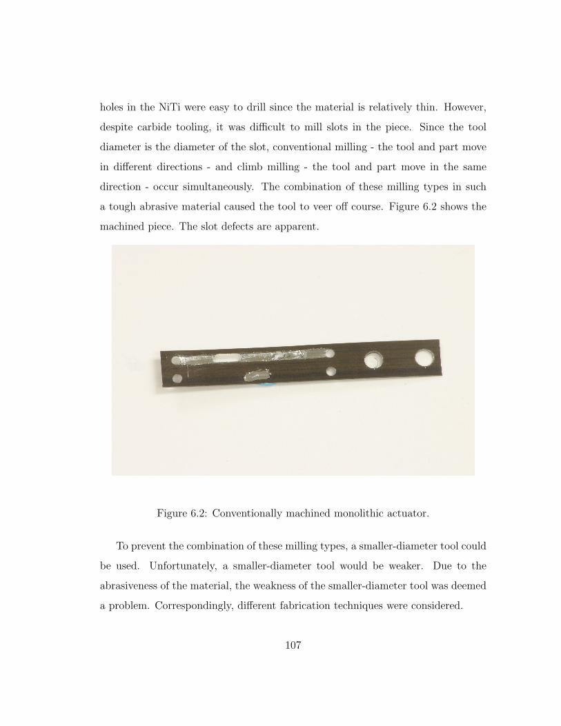
holes in the NiTi were easy to drill since the material is relatively thin. However,
despite carbide tooling, it was difficult to mill slots in the piece. Since the tool
diameter is the diameter of the slot, conventional milling - the tool and part move
in different directions - and climb milling - the tool and part move in the same
direction - occur simultaneously. The combination of these milling types in such
a tough abrasive material caused the tool to veer off course. Figure 6.2 shows the
machined piece. The slot defects are apparent.
Figure 6.2: Conventionally machined monolithic actuator.
To prevent the combination of these milling types, a smaller-diameter tool could
be used. Unfortunately, a smaller-diameter tool would be weaker. Due to the
abrasiveness of the material, the weakness of the smaller-diameter tool was deemed
a problem. Correspondingly, different fabrication techniques were considered.
107

An alternative to using the mill is to drill sequences of holes in a row to ob-
tain slots. With this method, jagged edges would remain where drilled holes were
removed. It would be difficult to make these rough insides smooth.
Other actuator fabrication techniques were considered due to the failure of con-
ventional machining to obtain the desired actuator prototype. After considering
electrical discharge machining (EDM), photochemical etching, laser cutting, and
waterjet cutting, waterjet cutting was seen as the best solution due to cost and
heat concerns.
In waterjet cutting, a machine pressurizes water into a narrow stream capable
of cutting and drilling many materials. For the monolithic actuator design, it is
critical to heat treat only the middle beam. With waterjet cutting, there is only a
small heat-affected zone. Figure 6.3 shows two waterjet-manufactured monolithic
actuators. Note the variation in the widths of the portal’s cantilever beams between
samples.
Now that the actuator shape has been manufactured from a single piece of NiTi,
it is necessary to develop a system to constrain the actuator in the appropriate
high-temperature shape while supplying heat only to the area that is to be locally
annealed.
6.2 Fixture Design and Heating Method
It is necessary to shape-set anneal the middle beam. To do this, it is imperative that
the middle beam be constrained in the desired shape and be annealed in this shape
by heating it to the annealing temperature Tanneal for an adequate amount of time.
It is also essential that the portal does not heat to Tanneal. In order to heat and
108

Figure 6.3: Waterjet-manufactured monolithic actuators.
109
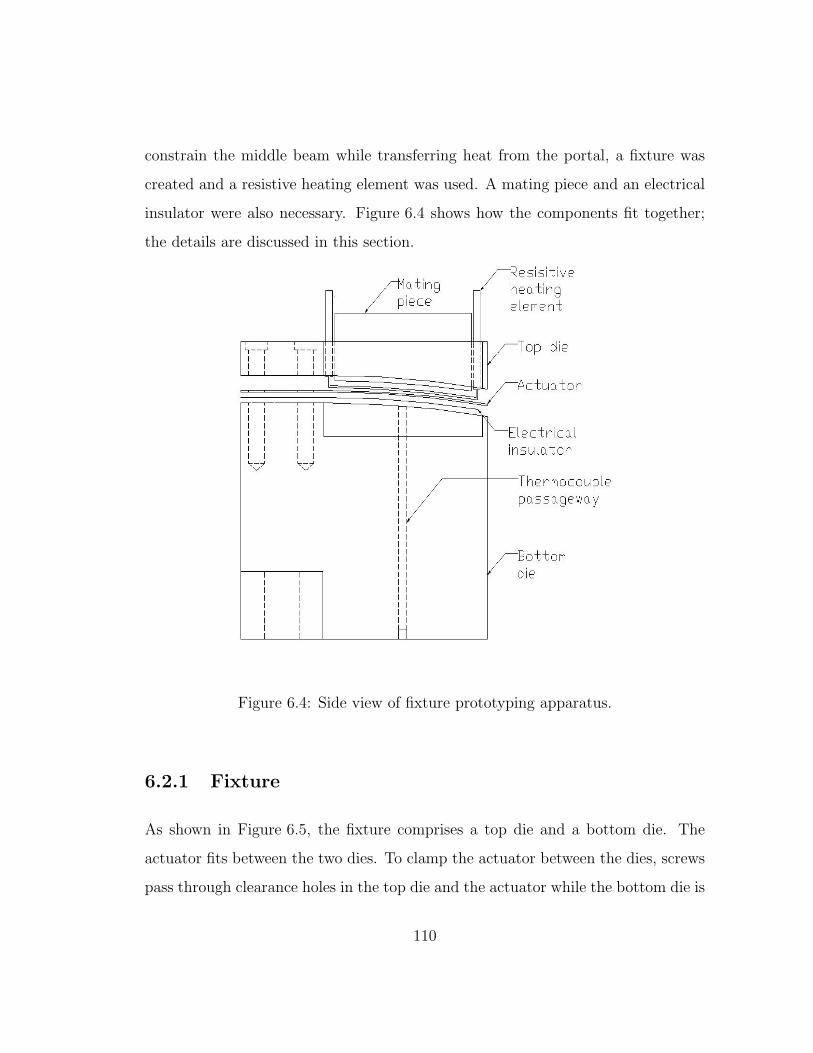
constrain the middle beam while transferring heat from the portal, a fixture was
created and a resistive heating element was used. A mating piece and an electrical
insulator were also necessary. Figure 6.4 shows how the components fit together;
the details are discussed in this section.
Figure 6.4: Side view of fixture prototyping apparatus.
6.2.1 Fixture
As shown in Figure 6.5, the fixture comprises a top die and a bottom die. The
actuator fits between the two dies. To clamp the actuator between the dies, screws
pass through clearance holes in the top die and the actuator while the bottom die is
110

tapped to receive them. Since both the top and bottom dies have the same radius
of curvature, the bottom die’s upper face fits with the top piece’s bottom face.
The dimensional drawings of the top and bottom dies are in Figures 6.6 and 6.7
respectively.
Figure 6.5: Fixture. The top and bottom dies are screwed together.
The dies are made from aluminium since aluminium has a good thermal con-
ductivity, is relatively cheap, and is easily machined. To fabricate these dies, it
was necessary to fillet and round some corners. To create the radius of curva-
ture in the bottom and top dies, MasterCAM software was used to make a file for
Computer-Numerical-Control machining.
While determining the annealing process, it was prudent to monitor the tem-
perature of the middle beam. Therefore, a hole for a thermocouple was made in
the bottom die at the mid-point of the arc length to enable this.
The bottom die has symmetric wings that each have a 14-20 clearance hole to
attach the die to a base plate if necessary.
111
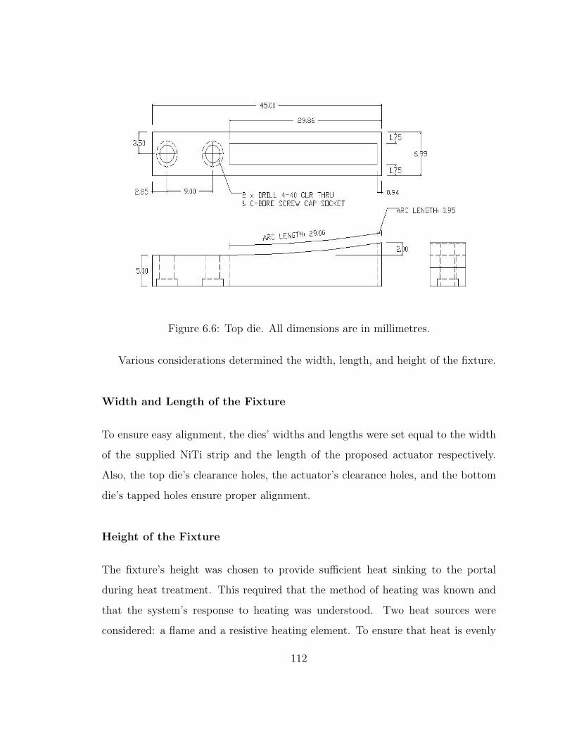
Figure 6.6: Top die. All dimensions are in millimetres.
Various considerations determined the width, length, and height of the fixture.
Width and Length of the Fixture
To ensure easy alignment, the dies’ widths and lengths were set equal to the width
of the supplied NiTi strip and the length of the proposed actuator respectively.
Also, the top die’s clearance holes, the actuator’s clearance holes, and the bottom
die’s tapped holes ensure proper alignment.
Height of the Fixture
The fixture’s height was chosen to provide sufficient heat sinking to the portal
during heat treatment. This required that the method of heating was known and
that the system’s response to heating was understood. Two heat sources were
considered: a flame and a resistive heating element. To ensure that heat is evenly
112

Figure 6.7: Bottom die. All dimensions are in millimetres.
113
applied, the resistive heating element in contact with the actuator was deemed
the best solution. To understand the system’s response to heating, finite element
analysis (FEA) was performed.
As shown in Figure 6.4, the resistive heating element is placed through a slot in
the top die. Power is supplied to the resistive heating element by attaching electrical
leads to the ends of the resistive heating element. This enables the heating element
to heat the beam through conduction. Conduction is the transfer of energy from
the more energetic to the less energetic particles of a substance due to interactions
between particles [7]. The conductive heat flux per unit area Qcond” is proportional
to the temperature gradient dTdx
and thermal conductivity k ( WmK
).
Qcond” = kdT
dx(6.1)
Using a thermally-insulated mating piece to push the resistive heating element
against the actuator and bottom die ensures that the middle beam maintains the
curvature as it anneals and reduces heat losses between the heating element and
NiTi by improving contact. The portal’s cantilever beams do not need to be shape-
set and must not anneal. Since the motion of the portal’s cantilever beams need
not be constricted as the device heats up, they are in contact with air instead of
the bottom die. As shown in Figure 6.5, this is done with side slots. The top die is
in contact with the portal’s cantilever beams to serve as a heat sink. The bottom
die’s height is greater than that of the top die to ensure heat transfer away from
the portal’s girder.
Other methods of heat transfer include convection and radiation. Convection is
used to cool the fixture while the resistive heating element heats the middle beam.
Since the fixture will be cooled with a fan, forced convection is the dominant mode
114
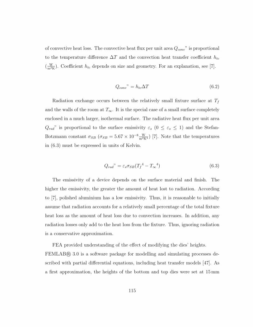
of convective heat loss. The convective heat flux per unit area Qconv” is proportional
to the temperature difference ∆T and the convection heat transfer coefficient htc
( Wm2K
). Coefficient htc depends on size and geometry. For an explanation, see [7].
Qconv” = htc∆T (6.2)
Radiation exchange occurs between the relatively small fixture surface at Tf
and the walls of the room at T∞. It is the special case of a small surface completely
enclosed in a much larger, isothermal surface. The radiative heat flux per unit area
Qrad” is proportional to the surface emissivity εs (0 ≤ εs ≤ 1) and the Stefan-
Botzmann constant σSB (σSB = 5.67× 10⁻⁸ Wm2K4 ) [7]. Note that the temperatures
in (6.3) must be expressed in units of Kelvin.
Qrad” = εsσSB(Tf4 − T∞
4) (6.3)
The emissivity of a device depends on the surface material and finish. The
higher the emissivity, the greater the amount of heat lost to radiation. According
to [7], polished aluminium has a low emissivity. Thus, it is reasonable to initially
assume that radiation accounts for a relatively small percentage of the total fixture
heat loss as the amount of heat loss due to convection increases. In addition, any
radiation losses only add to the heat loss from the fixture. Thus, ignoring radiation
is a conservative approximation.
FEA provided understanding of the effect of modifying the dies’ heights.
FEMLAB r© 3.0 is a software package for modelling and simulating processes de-
scribed with partial differential equations, including heat transfer models [47]. As
a first approximation, the heights of the bottom and top dies were set at 15mm
115

and 8mm respectively. The space dimension was three-dimensional and the appli-
cation mode was “heat transfer through conduction with heat flux, convective, and
temperature boundary conditions”. A plane of symmetry bisects the fixture width
along the length to reduce the model to half its size.
To perform the simulations, four subdomains were created. They were the
top die, bottom die, actuator middle beam, and portal. The thermal conductiv-
ity, density, and heat capacity of the top and bottom dies correspond to those of
aluminium. They were 237 WmK
, 2702 kgm3 , and 903 J
kgKrespectively [7]. Since the
austenite value for density is unknown, the martensite value for density is used for
the middle beam. The density and specific heat of the actuator middle beam are
listed in Table 4.2. The thermal conductivity for the middle beam was set at that
of austenite, 18 WmK
[27]. Since the density and specific heat for as-rolled NiTi are
unknown, these properties were set to the same values of those of the actuator’s
middle beam. The thermal conductivity for the desired non-annealed section is set
to that of martensite, 8.6 WmK
[27]. For the simulations, the external temperature
was set to 293K and the convection heat transfer coefficient was set at 125 Wm2K
.
The convection heat transfer coefficient was obtained from [7] assuming forced gas
convection.
While performing these simulations, the dies’ curvatures were ignored to reduce
the mesh size by simplifying the geometry. Also, as an initial simulation condition,
the middle beam is set to the same temperature as the resistive heating element,
773K. This temperature corresponds with Tanneal [48]. Since the actuator is thin,
it was assumed that the middle beam will heat up almost instantaneously by con-
duction.
According to [48], it may take less than one minute in a heated die to anneal
a small piece. Since the thickness of the actuator is small, it was assumed that
116
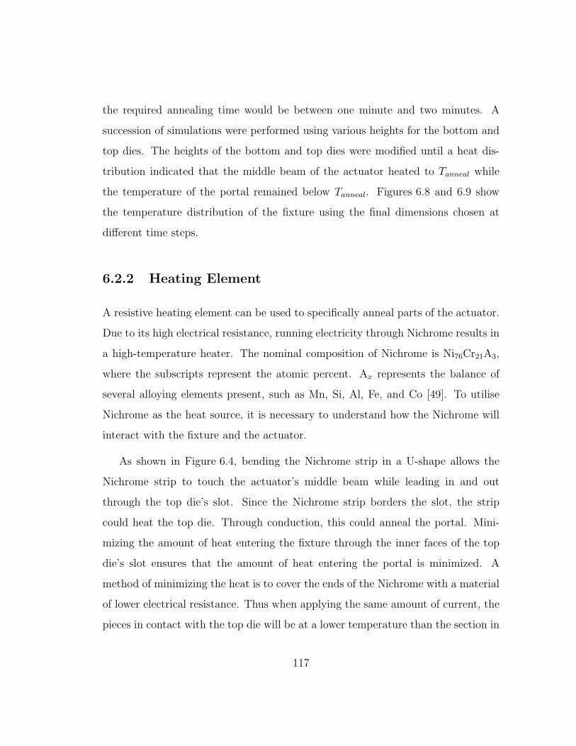
the required annealing time would be between one minute and two minutes. A
succession of simulations were performed using various heights for the bottom and
top dies. The heights of the bottom and top dies were modified until a heat dis-
tribution indicated that the middle beam of the actuator heated to Tanneal while
the temperature of the portal remained below Tanneal. Figures 6.8 and 6.9 show
the temperature distribution of the fixture using the final dimensions chosen at
different time steps.
6.2.2 Heating Element
A resistive heating element can be used to specifically anneal parts of the actuator.
Due to its high electrical resistance, running electricity through Nichrome results in
a high-temperature heater. The nominal composition of Nichrome is Ni76Cr21A3,
where the subscripts represent the atomic percent. Ax represents the balance of
several alloying elements present, such as Mn, Si, Al, Fe, and Co [49]. To utilise
Nichrome as the heat source, it is necessary to understand how the Nichrome will
interact with the fixture and the actuator.
As shown in Figure 6.4, bending the Nichrome strip in a U-shape allows the
Nichrome strip to touch the actuator’s middle beam while leading in and out
through the top die’s slot. Since the Nichrome strip borders the slot, the strip
could heat the top die. Through conduction, this could anneal the portal. Mini-
mizing the amount of heat entering the fixture through the inner faces of the top
die’s slot ensures that the amount of heat entering the portal is minimized. A
method of minimizing the heat is to cover the ends of the Nichrome with a material
of lower electrical resistance. Thus when applying the same amount of current, the
pieces in contact with the top die will be at a lower temperature than the section in
117
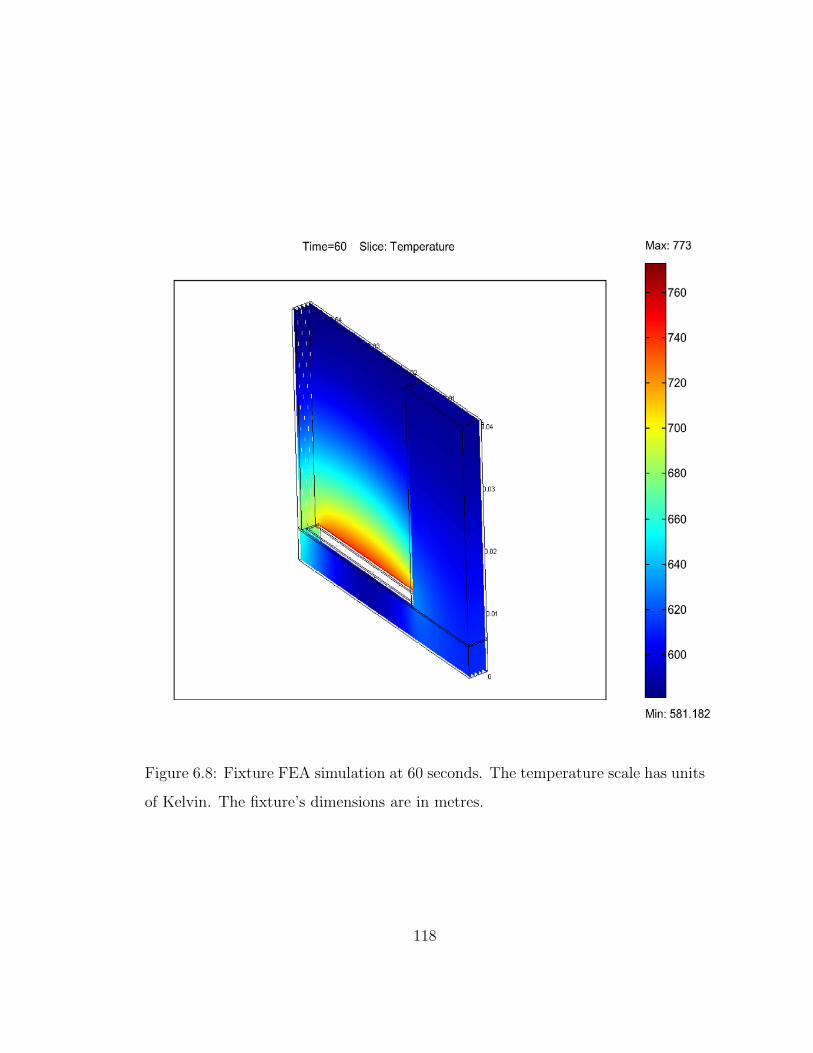
Figure 6.8: Fixture FEA simulation at 60 seconds. The temperature scale has units
of Kelvin. The fixture’s dimensions are in metres.
118
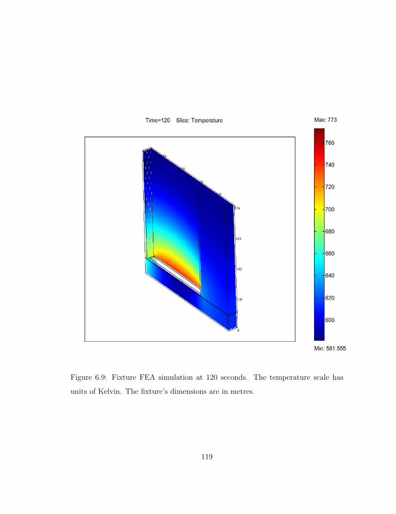
Figure 6.9: Fixture FEA simulation at 120 seconds. The temperature scale has
units of Kelvin. The fixture’s dimensions are in metres.
119
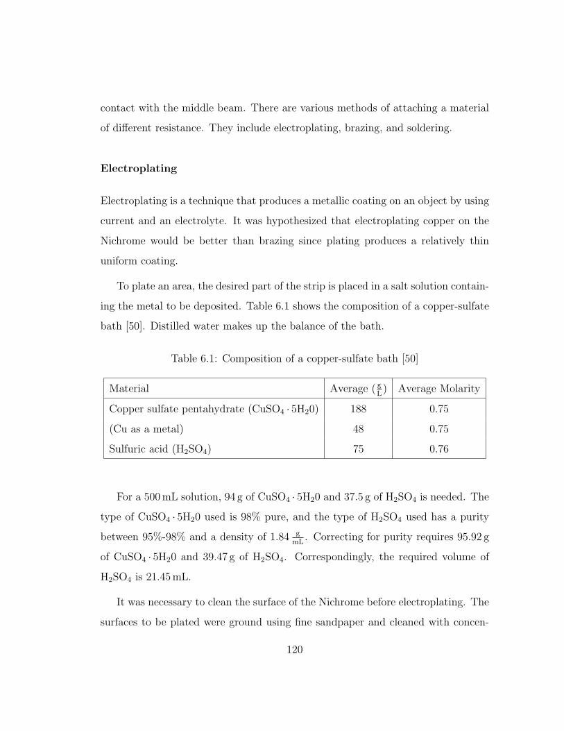
contact with the middle beam. There are various methods of attaching a material
of different resistance. They include electroplating, brazing, and soldering.
Electroplating
Electroplating is a technique that produces a metallic coating on an object by using
current and an electrolyte. It was hypothesized that electroplating copper on the
Nichrome would be better than brazing since plating produces a relatively thin
uniform coating.
To plate an area, the desired part of the strip is placed in a salt solution contain-
ing the metal to be deposited. Table 6.1 shows the composition of a copper-sulfate
bath [50]. Distilled water makes up the balance of the bath.
Table 6.1: Composition of a copper-sulfate bath [50]
Material Average ( gL) Average Molarity
Copper sulfate pentahydrate (CuSO4 · 5H20) 188 0.75
(Cu as a metal) 48 0.75
Sulfuric acid (H2SO4) 75 0.76
For a 500mL solution, 94 g of CuSO4 · 5H20 and 37.5 g of H2SO4 is needed. The
type of CuSO4 · 5H20 used is 98% pure, and the type of H2SO4 used has a purity
between 95%-98% and a density of 1.84 gmL
. Correcting for purity requires 95.92 g
of CuSO4 · 5H20 and 39.47 g of H2SO4. Correspondingly, the required volume of
H2SO4 is 21.45mL.
It was necessary to clean the surface of the Nichrome before electroplating. The
surfaces to be plated were ground using fine sandpaper and cleaned with concen-
120
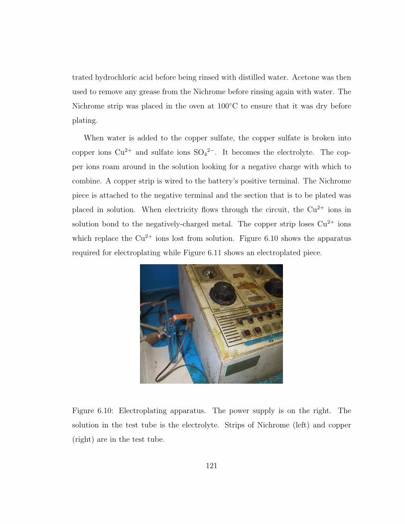
trated hydrochloric acid before being rinsed with distilled water. Acetone was then
used to remove any grease from the Nichrome before rinsing again with water. The
Nichrome strip was placed in the oven at 100C to ensure that it was dry before
plating.
When water is added to the copper sulfate, the copper sulfate is broken into
copper ions Cu2+ and sulfate ions SO42−. It becomes the electrolyte. The cop-
per ions roam around in the solution looking for a negative charge with which to
combine. A copper strip is wired to the battery’s positive terminal. The Nichrome
piece is attached to the negative terminal and the section that is to be plated was
placed in solution. When electricity flows through the circuit, the Cu2+ ions in
solution bond to the negatively-charged metal. The copper strip loses Cu2+ ions
which replace the Cu2+ ions lost from solution. Figure 6.10 shows the apparatus
required for electroplating while Figure 6.11 shows an electroplated piece.
Figure 6.10: Electroplating apparatus. The power supply is on the right. The
solution in the test tube is the electrolyte. Strips of Nichrome (left) and copper
(right) are in the test tube.
121

Figure 6.11: Electroplated strip of Nichrome.
122
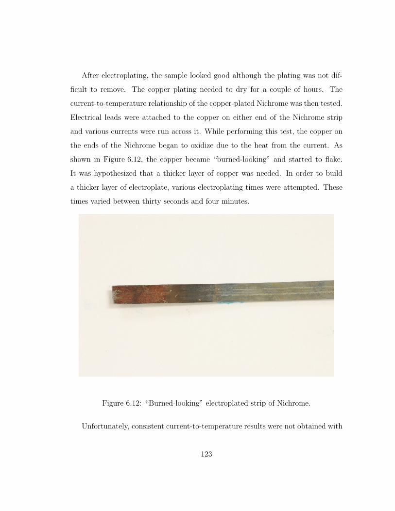
After electroplating, the sample looked good although the plating was not dif-
ficult to remove. The copper plating needed to dry for a couple of hours. The
current-to-temperature relationship of the copper-plated Nichrome was then tested.
Electrical leads were attached to the copper on either end of the Nichrome strip
and various currents were run across it. While performing this test, the copper on
the ends of the Nichrome began to oxidize due to the heat from the current. As
shown in Figure 6.12, the copper became “burned-looking” and started to flake.
It was hypothesized that a thicker layer of copper was needed. In order to build
a thicker layer of electroplate, various electroplating times were attempted. These
times varied between thirty seconds and four minutes.
Figure 6.12: “Burned-looking” electroplated strip of Nichrome.
Unfortunately, consistent current-to-temperature results were not obtained with
123
electroplating. When the copper plating was too thin, all the current passing
through the layer became too much for the copper to handle. Increasing the time
for electroplating led to a thicker coating. However, the contact resistance between
the Nichrome and copper layer became too great and sparks occurred between the
leads. To achieve a satisfactory coating, it may have been necessary to use an
additive in the solution [50]. Instead of investigating this avenue, it was decided to
look into brazing.
Brazing
Brazing is a technique used to join two metals. Thus, another option is brazing a
piece of copper to a Nichrome strip. Copper is an excellent conductor of electricity
and is readily available. Silver-tin solder was used to join the materials. Figure 6.13
shows the piece.
Tests were done to understand the current-to-temperature relationship of copper-
brazed Nichrome. Non-conductive vices clamped the strip of Nichrome. Electrical
leads and a variable direct-current power supply were used to heat the Nichrome.
As the current varied, a thermocouple at the strip’s mid-length allowed manual
recording of the temperature. Figure 6.14 shows various tests performed using an
approximately 62mm-long, 2mm-wide, 0.3mm-thick Nichrome strip.
These tests illustrate a consistent, almost-linear relationship between tempera-
ture and current. If it is desired to heat a Nichrome strip to a certain temperature,
it is possible to use this figure to determine an appropriate input current.
The easily-available copper strips have an approximate thickness of 0.75mm.
After brazing, the copper-brazed Nichrome strip has a maximum thickness of
1.36mm including the thickness added as a result of the silver-tin solder. Also,
124
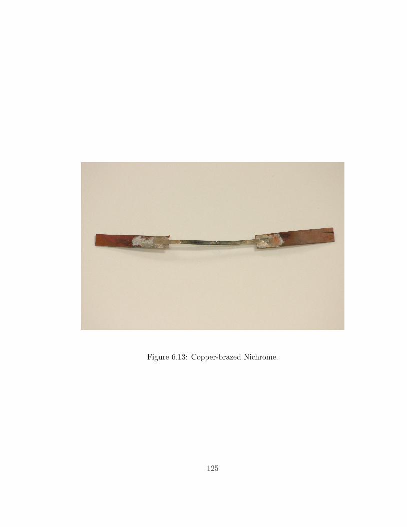
Figure 6.13: Copper-brazed Nichrome.
125

0
100
200
300
400
500
600
700
800
0 2 4 6 8 10 12 14 16
current (A)
tem
pera
tue
(°C
)
test 1test 2test 3test 4
Figure 6.14: Temperature of a copper-brazed Nichrome strip.
126

the width of the copper strips need to be greater than that of the Nichrome strip
to make them easier to join. Figure 6.13 shows the Nichrome and copper mating
on one face. In this scenario, the face of the Nichrome not attached to copper is
exposed to its surroundings where it is not covered in blotches of solder. Also, the
copper-brazed Nichrome strip is appreciably wider and thicker at the union of the
components. As the resistive heating element becomes wider and thicker, it be-
comes more difficult to place within the fixture. As a result, using silver-tin solder
as the material of lesser resistance is investigated next.
Soldering
The third option was to cover the Nichrome ends with silver-tin solder. Experimen-
tal results were obtained to understand the current-to-temperature relationship for
a piece of Nichrome with silver-tin solder at its ends. Non-conductive vices clamped
the strip of Nichrome. Electrical leads and a variable direct-current power supply
were used to heat the Nichrome. As the current varied, a thermocouple at the strip’s
mid-length allowed manual recording of the temperature. Another thermocouple
was placed between mid-length and one silver-tin soldered end. This thermocouple
was used to ensure that the temperature gradient along the strip was not significant.
Figures 6.15 and 6.16 show the set-up.
Figure 6.17 shows the current-to-temperature relationship of a strip having an
approximate length, width, and thickness of 33.0mm, 2.0mm, and 0.3mm respec-
tively. The thermocouple had a fused bead and was welded mid-length on the
Nichrome strip. The alligator clips made contact with the silver-tin solder at the
strip’s ends. Note that the thermocouple acts like a heat fin so the temperature of
the Nichrome strip is expected to be higher than recorded.
127

Figure 6.15: Experimental set-up for silver-tin end-soldered Nichrome strip current-
to-temperature test. The 20A direct-current power supply is on the left. The
vices holding the Nichrome strip are on the right above the Omega HH501DK
thermometer.
Figure 6.16: Thermocouples and electrical leads on silver-tin end-soldered Nichrome
strip.
128

0
100
200
300
400
500
600
700
0 2 4 6 8 10 12 14current (A)
tem
per
atu
re (
°C)
test 1test 2
Figure 6.17: Temperature of a silver-tin end-soldered Nichrome strip.
129
Figure 6.17 illustrates a consistent, almost-linear relationship between current
and temperature. These current-to-temperature results are similar to those of
the copper-brazed Nichrome strip in Figure 6.14. This indicates that whether the
Nichrome strip has copper-brazed ends or silver-tin soldered ends, the current-to-
temperature relationship is not significantly affected. Given this and the fact that
silver-tin solder ends are thinner than copper-brazed Nichrome ends, silver-tin sol-
der was used to plate the section of Nichrome that contacts the inner surfaces of
the top die.
Heat Consistency
It is important to understand the heat distribution across the resistive heating
element. Some resistive heating elements have a 10F to 20F temperature variation
across their length [51]. Since little information is available about the heat strips
provided, monitoring heat consistency was done with spot-welded thermocouples.
Generally, the strip’s temperature should be consistent along its length. How-
ever, within approximately 5mm of where the solder ends, there is a region where
the temperature varies significantly. In one experiment, three thermocouples were
welded to the strip - one was attached on the solder near the electrical lead, one
was on the Nichrome next to the solder, and the other was at the mid-length of
the strip. The strip had a length, width, and thickness of 76.0mm, 1.9mm, and
0.3mm respectively.
During this experiment, it was noted that the temperature recorded by the ther-
mocouple on the solder was significantly lower than the temperature recorded by the
mid-strip thermocouple. The thermocouple between the other two thermocouples
measured a temperature between the others’ values.
130
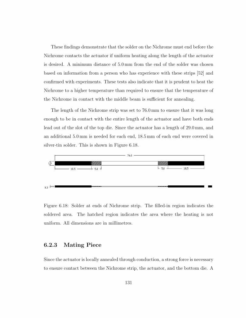
These findings demonstrate that the solder on the Nichrome must end before the
Nichrome contacts the actuator if uniform heating along the length of the actuator
is desired. A minimum distance of 5.0mm from the end of the solder was chosen
based on information from a person who has experience with these strips [52] and
confirmed with experiments. These tests also indicate that it is prudent to heat the
Nichrome to a higher temperature than required to ensure that the temperature of
the Nichrome in contact with the middle beam is sufficient for annealing.
The length of the Nichrome strip was set to 76.0mm to ensure that it was long
enough to be in contact with the entire length of the actuator and have both ends
lead out of the slot of the top die. Since the actuator has a length of 29.0mm, and
an additional 5.0mm is needed for each end, 18.5mm of each end were covered in
silver-tin solder. This is shown in Figure 6.18.
Figure 6.18: Solder at ends of Nichrome strip. The filled-in region indicates the
soldered area. The hatched region indicates the area where the heating is not
uniform. All dimensions are in millimetres.
6.2.3 Mating Piece
Since the actuator is locally annealed through conduction, a strong force is necessary
to ensure contact between the Nichrome strip, the actuator, and the bottom die. A
131

greater force results in a greater pressure that reduces contact resistance. Reducing
contact resistance improves heat transfer. Pushing a mating piece against the
Nichrome strip helps provide the necessary force to keep the strip, middle beam, and
bottom die in contact. The mating piece’s material must have excellent temperature
resistance, be suitable for continuous use at 800C, be machinable, have minimal
thermal expansion, and be an electrical and thermal insulator. Given these desired
material qualities, MACOR r© Machinable Glass Ceramic was chosen [53].
This mating piece needs to have the same radius of curvature as the top die.
To ensure that it fits into the slot with the solder-plated Nichrome, its arc length
needs to be less than the length of the actuator’s middle beam. Let the radius of
curvature be 223.92mm for the top die, bottom die, and the mating piece. Assume
that the top die’s arc length begins at the bottom dead center of a circle that
corresponds with 0. Then let the start arc angle and finish arc angle of the mating
piece equal 0.36 and 7.06 respectively. Figure 6.19 shows the dimensions of the
machined ceramic. To machine ceramic, it is necessary to use carbide tooling and
to keep the piece cool.
Figure 6.19: Ceramic mating piece. All dimensions are in millimetres.
132

The expansion of the ceramic must also be considered during the heat-treatment
process. According to [53], the ceramic’s coefficient of expansion is 94× 10−7 ininC
which is less than that of aluminium. Thus as the jig heats up, the ceramic will
not expand more than the aluminium fixture.
6.2.4 Electrical Insulator
It is necessary that the resistive heating element be electrically insulated from the
aluminium fixture so that current does not flow through the fixture. The material
required must be an electrical insulator and be able to operate at 600C. Thermally
conductive tape is one option.
Kapton r©, produced by DuPontTM, is an electrically insulating tape. However,
it is typically used in applications that range between -269C and 400C [54]. A
temperature drop due to the thermal contact resistance of Kapton r© is estimated
by a temperature difference ranging between 50C and 70C [52]. Its thermal
conductivity is quite low at 0.12 WmK
[55]. However, it was readily available at no
cost.
Kapton r© tape was placed in the inner faces of the top die’s slot and on the
upper face of the bottom die that is in contact with the middle beam. This insulates
the fixture from the electrical source. Note that the actuator is not electrically
insulated. Electrically insulating the actuator from the heat source would result
in a temperature drop due to thermal contact resistance between the Nichrome
and Kapton r© interface and between the Kapton r© and actuator interface. Note
that an electrically-insulating and thermally-conductive material would have been
better to insulate the bottom die from the Nichrome while still allowing‘ heat to
conduct through its surface.
133
6.2.5 Fixture Design and Heating Method Summary
This section detailed the design of the fixture used to shape-set the middle beam and
other necessary components for this process. Nichrome is chosen as the resistive
heating element to supply the necessary energy to anneal the middle beam. A
mating piece is designed to ensure contact between the Nichrome strip, middle
actuator beam, and bottom die. Kapton r© is the material that electrically insulates
the aluminium fixture from the Nichrome. Now that the actuator, fixture, and other
necessary components for the local anneal have been manufactured, it is important
to determine the middle beam shape-setting process.
6.3 Middle Beam Shape-Setting Process
Now that the fixture necessary for constraining the middle beam in its high-
temperature shape is specified, defining the heat-treatment process is required.
According to [48], the NiTi annealing temperature should be between 500C
and 550C. The material requiring annealing must reach this desired temperature
throughout its cross-section during the heat-treatment process. It is expected that
since the actuator is thin, the annealed beam will heat up almost instantaneously
by conduction. For a small piece, it may take less than one minute to anneal in a
heated die whereas it may take ten minutes to twenty minutes to heat a larger fixture
in a furnace [48]. Thus, it is paramount to have a thermocouple monitoring the
temperature of the actuator until the process is perfected. A thermocouple is used
to monitor the temperature of the actuator’s face in contact with the bottom die.
While heat treating the middle beam, it is also crucial to examine the temperature
of the girder. If the girder heats up, heat transfers to the portal’s cantilever beams
134
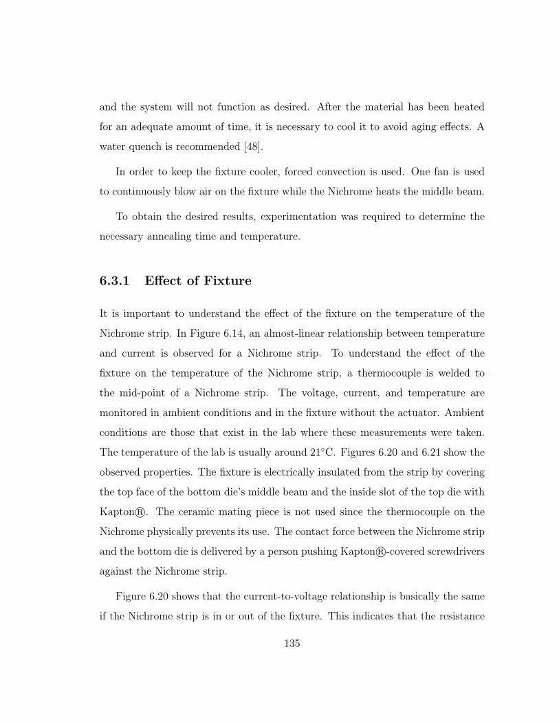
and the system will not function as desired. After the material has been heated
for an adequate amount of time, it is necessary to cool it to avoid aging effects. A
water quench is recommended [48].
In order to keep the fixture cooler, forced convection is used. One fan is used
to continuously blow air on the fixture while the Nichrome heats the middle beam.
To obtain the desired results, experimentation was required to determine the
necessary annealing time and temperature.
6.3.1 Effect of Fixture
It is important to understand the effect of the fixture on the temperature of the
Nichrome strip. In Figure 6.14, an almost-linear relationship between temperature
and current is observed for a Nichrome strip. To understand the effect of the
fixture on the temperature of the Nichrome strip, a thermocouple is welded to
the mid-point of a Nichrome strip. The voltage, current, and temperature are
monitored in ambient conditions and in the fixture without the actuator. Ambient
conditions are those that exist in the lab where these measurements were taken.
The temperature of the lab is usually around 21C. Figures 6.20 and 6.21 show the
observed properties. The fixture is electrically insulated from the strip by covering
the top face of the bottom die’s middle beam and the inside slot of the top die with
Kapton r©. The ceramic mating piece is not used since the thermocouple on the
Nichrome physically prevents its use. The contact force between the Nichrome strip
and the bottom die is delivered by a person pushing Kapton r©-covered screwdrivers
against the Nichrome strip.
Figure 6.20 shows that the current-to-voltage relationship is basically the same
if the Nichrome strip is in or out of the fixture. This indicates that the resistance
135
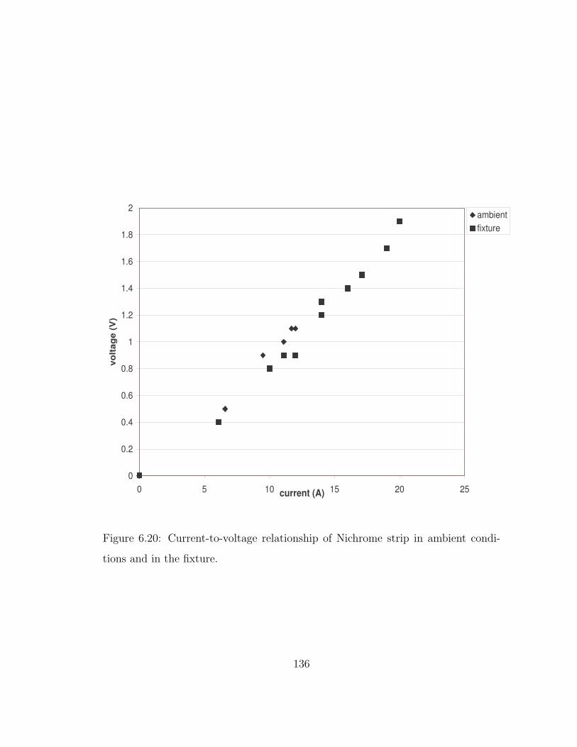
0
0.2
0.4
0.6
0.8
1
1.2
1.4
1.6
1.8
2
0 5 10 15 20 25current (A)
volt
age
(V)
ambientfixture
Figure 6.20: Current-to-voltage relationship of Nichrome strip in ambient condi-
tions and in the fixture.
136
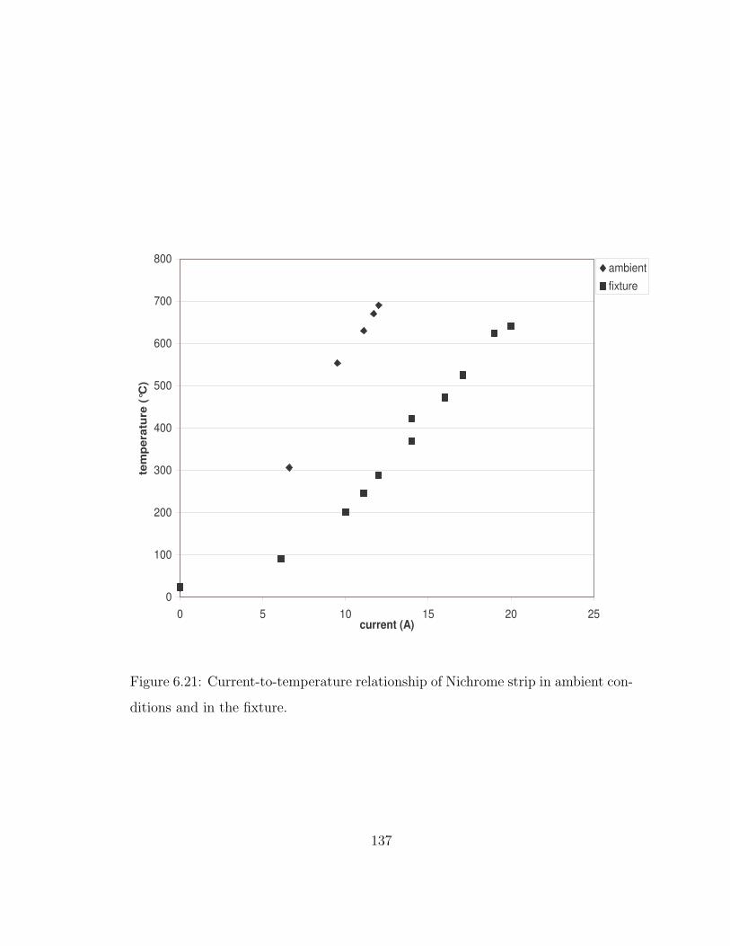
0
100
200
300
400
500
600
700
800
0 5 10 15 20 25current (A)
tem
per
atu
re (
°C)
ambientfixture
Figure 6.21: Current-to-temperature relationship of Nichrome strip in ambient con-
ditions and in the fixture.
137

does not change. However, Figure 6.21 shows that the amount of current required
for a specific temperature depends on whether the Nichrome strip is in the fixture or
if it is exposed to ambient conditions. This is a result of heat transfer being greater
due to conduction in the fixture than free convection in ambient conditions. Due
to the heat sinking, it takes more power to get to the same temperature because
some heat is lost to the fixture.
6.3.2 Effect of Forced Convection
One must also understand the effect of forced convection on the temperatures of
the Nichrome strip, the mid-length of the middle beam, and the tip of the middle
beam when the Nichrome strip is in the fixture. To comprehend forced convection,
thermocouples are welded at the mid-length of the Nichrome strip, the mid-length
of the actuator’s middle beam, and at the tip of the annealed beam to enable
the monitoring of temperature and current. Figures 6.22, 6.23, and 6.24 show the
results from this series of experiments. The fixture is electrically insulated from the
Nichrome strip by covering the top face of the bottom die’s middle beam and the
inside slot of the top die with Kapton r©. The ceramic mating piece is not used since
the thermocouple on the Nichrome physically prevents its use. The contact force
between the Nichrome strip and the bottom die is delivered by a person pushing
Kapton r©-covered screwdrivers against the Nichrome strip.
Figure 6.22 shows that the current-to-temperature relationship of the same
Nichrome strip in a fixture is basically the same regardless of the presence of forced
convection applied in the x-direction. Figures 6.23 and 6.24 show that the amount
of current required for a specific temperature at the mid-point or at the end-point
of the middle beam depends on the presence of forced convection. Since the fan-
138

0
100
200
300
400
500
600
700
800
900
1000
0 5 10 15 20 25current (A)
tem
per
atu
re (
°C)
freeforced
Figure 6.22: Current-to-temperature relationship of Nichrome strip in fixture with
free and forced convection.
139
0
50
100
150
200
250
300
350
400
450
0 5 10 15 20 25current (A)
tem
per
atu
re (
°C)
freeforced
Figure 6.23: Current-to-temperature relationship of middle beam mid-point with
free and forced convection. The actuator is in the fixture.
140
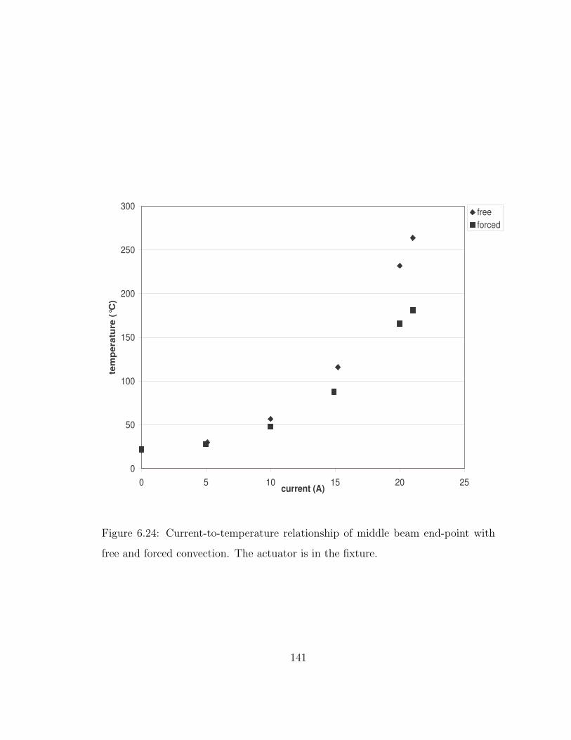
0
50
100
150
200
250
300
0 5 10 15 20 25current (A)
tem
per
atu
re (
°C)
freeforced
Figure 6.24: Current-to-temperature relationship of middle beam end-point with
free and forced convection. The actuator is in the fixture.
141
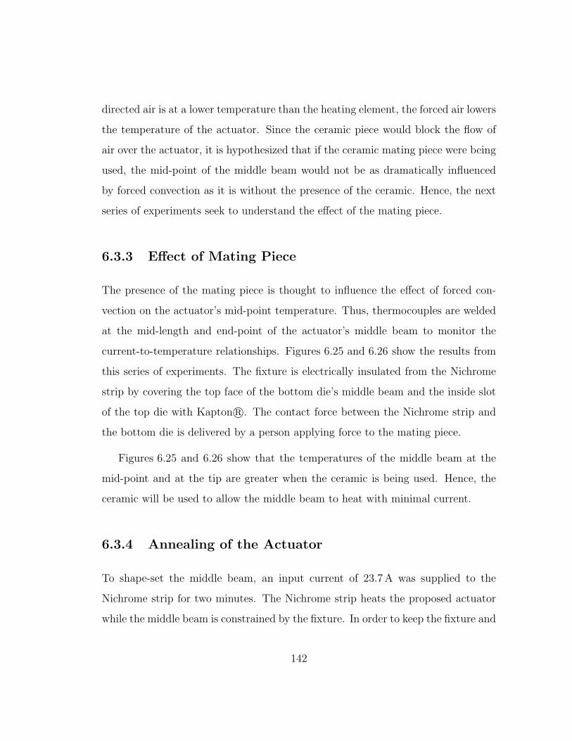
directed air is at a lower temperature than the heating element, the forced air lowers
the temperature of the actuator. Since the ceramic piece would block the flow of
air over the actuator, it is hypothesized that if the ceramic mating piece were being
used, the mid-point of the middle beam would not be as dramatically influenced
by forced convection as it is without the presence of the ceramic. Hence, the next
series of experiments seek to understand the effect of the mating piece.
6.3.3 Effect of Mating Piece
The presence of the mating piece is thought to influence the effect of forced con-
vection on the actuator’s mid-point temperature. Thus, thermocouples are welded
at the mid-length and end-point of the actuator’s middle beam to monitor the
current-to-temperature relationships. Figures 6.25 and 6.26 show the results from
this series of experiments. The fixture is electrically insulated from the Nichrome
strip by covering the top face of the bottom die’s middle beam and the inside slot
of the top die with Kapton r©. The contact force between the Nichrome strip and
the bottom die is delivered by a person applying force to the mating piece.
Figures 6.25 and 6.26 show that the temperatures of the middle beam at the
mid-point and at the tip are greater when the ceramic is being used. Hence, the
ceramic will be used to allow the middle beam to heat with minimal current.
6.3.4 Annealing of the Actuator
To shape-set the middle beam, an input current of 23.7A was supplied to the
Nichrome strip for two minutes. The Nichrome strip heats the proposed actuator
while the middle beam is constrained by the fixture. In order to keep the fixture and
142
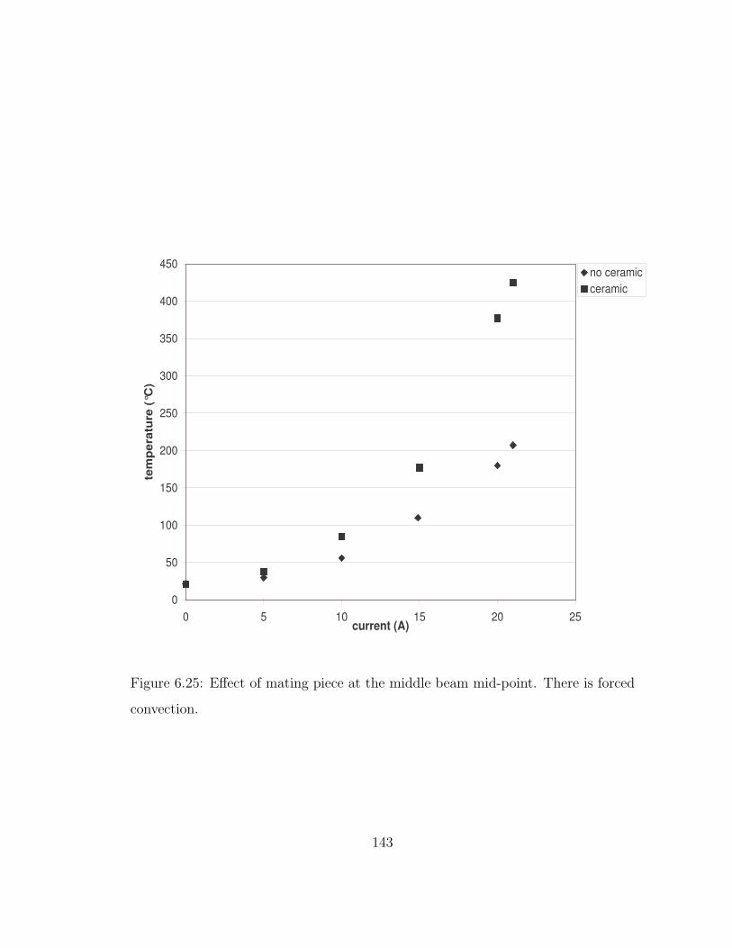
0
50
100
150
200
250
300
350
400
450
0 5 10 15 20 25current (A)
tem
per
atu
re (
°C)
no ceramicceramic
Figure 6.25: Effect of mating piece at the middle beam mid-point. There is forced
convection.
143

0
50
100
150
200
250
0 5 10 15 20 25current (A)
tem
per
atu
re (
°C)
no ceramicceramic
Figure 6.26: Effect of mating piece at the middle beam end-point. There is forced
convection.
144

girder cooler, a fan was used to continuously blow air. The ceramic mating piece
is used to allow the middle beam to heat with minimal current. The effectiveness
of this shape-setting process is investigated in the next chapter.
6.3.5 Monolithic Prototype Summary
This section outlined the process used to determine the middle beam shape-setting
process. It is important to confirm that this shape-setting process works. Thus,
the following chapter is dedicated to testing the prototype.
145

Chapter 7
Prototype Testing
To determine if the shape-set and heat-treatment process was successful, the post-
treated nature of the actuator needed assessment. This chapter focuses on the
prototyping of two samples, SA and SB. By examining the macroscopic behaviour
of the samples, it is possible to determine the degree of local annealing achieved.
This chapter also investigates the use of electrical current to actuator a sample SC .
An attempt to examine the microstructure of the actuator is also discussed.
Before annealing, but after machining, the samples had an initial curvature.
This curvature is visible in the bottom sample shown in Figures 7.1 and 7.2, and
could be a result of the residual stress in the material. This residual stress may have
been introduced during the rolling stage of fabrication, the coiled storage position,
or the waterjet fabrication process. If one tried to deflect the tip of the sample, it
would elastically return to its initial shape.
The non-annealed samples were placed in the fixture so that their ends pointed
toward the top die. This was to ensure that any shape-set after annealing was not
a product of residual stresses from a prior process, but due to the anneal. The
146
samples were constrained in the fixture detailed in Chapter 6 and annealed for two
minutes. An input current of 23.7A was supplied to the Nichrome strip.
The dimensions of SB were recorded before and after annealing. The middle
beam of the actuator shrunk appreciably during annealing while the portal’s can-
tilever beams did not. The residual stresses stored in the material are relieved with
the heat treatment. It is hypothesized that this relief anneal causes the middle
beam to shrink. Thus, the shrinking of the middle beam demonstrates that the
middle beam is heated more than the portal’s cantilever beams.
After annealing, the sample has two stable states due to the buckling of the
portal’s cantilever beams. Figures 7.1 and 7.2 show SB before annealing (bottom)
and SA after annealing (top). Note that in Figure 7.1, an upward external force
was applied at the tips’ ends. In Figure 7.2, a downward external force was applied
at the tips’ ends. Regardless of the direction of the external force, the non-annealed
sample returns to the same equilibrium position while the annealed sample has two
equilibrium positions at low temperature. The annealed states are known as the
direction of anneal state and the direction opposite anneal state. If the curvature of
the sample is in the direction of the bottom die’s curvature then the sample is in the
direction of anneal state. If the curvature of the sample is in the direction opposite
the bottom die’s curvature then the sample is in the direction opposite anneal state.
The annealed sample is in the direction opposite anneal state in Figure 7.1 while
the annealed sample is in the direction of anneal state in Figure 7.2.
To better understand the effects of the annealing process, the behaviour of the
actuator, the middle beam, and the portal are examined.
147
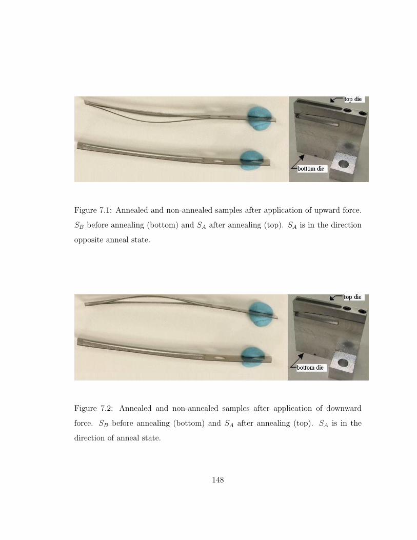
Figure 7.1: Annealed and non-annealed samples after application of upward force.
SB before annealing (bottom) and SA after annealing (top). SA is in the direction
opposite anneal state.
Figure 7.2: Annealed and non-annealed samples after application of downward
force. SB before annealing (bottom) and SA after annealing (top). SA is in the
direction of anneal state.
148
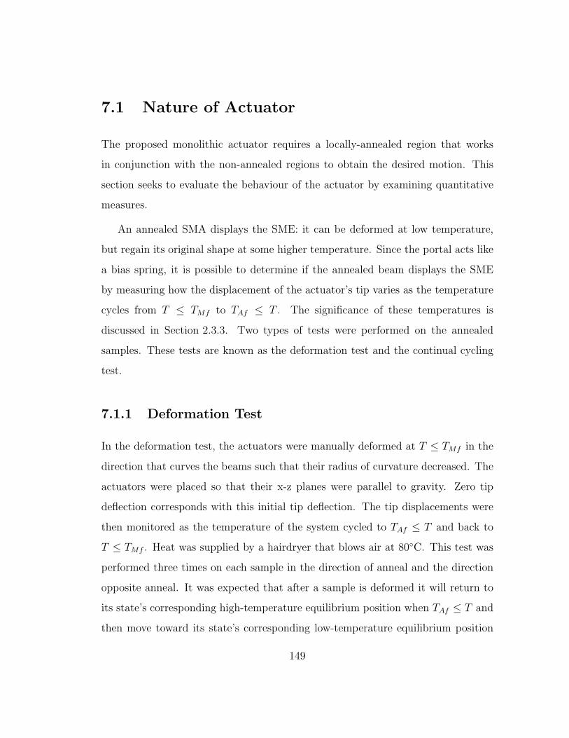
7.1 Nature of Actuator
The proposed monolithic actuator requires a locally-annealed region that works
in conjunction with the non-annealed regions to obtain the desired motion. This
section seeks to evaluate the behaviour of the actuator by examining quantitative
measures.
An annealed SMA displays the SME: it can be deformed at low temperature,
but regain its original shape at some higher temperature. Since the portal acts like
a bias spring, it is possible to determine if the annealed beam displays the SME
by measuring how the displacement of the actuator’s tip varies as the temperature
cycles from T ≤ TMf to TAf ≤ T . The significance of these temperatures is
discussed in Section 2.3.3. Two types of tests were performed on the annealed
samples. These tests are known as the deformation test and the continual cycling
test.
7.1.1 Deformation Test
In the deformation test, the actuators were manually deformed at T ≤ TMf in the
direction that curves the beams such that their radius of curvature decreased. The
actuators were placed so that their x-z planes were parallel to gravity. Zero tip
deflection corresponds with this initial tip deflection. The tip displacements were
then monitored as the temperature of the system cycled to TAf ≤ T and back to
T ≤ TMf . Heat was supplied by a hairdryer that blows air at 80C. This test was
performed three times on each sample in the direction of anneal and the direction
opposite anneal. It was expected that after a sample is deformed it will return to
its state’s corresponding high-temperature equilibrium position when TAf ≤ T and
then move toward its state’s corresponding low-temperature equilibrium position
149
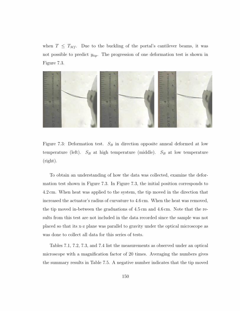
when T ≤ TMf . Due to the buckling of the portal’s cantilever beams, it was
not possible to predict ytip. The progression of one deformation test is shown in
Figure 7.3.
Figure 7.3: Deformation test. SB in direction opposite anneal deformed at low
temperature (left). SB at high temperature (middle). SB at low temperature
(right).
To obtain an understanding of how the data was collected, examine the defor-
mation test shown in Figure 7.3. In Figure 7.3, the initial position corresponds to
4.2 cm. When heat was applied to the system, the tip moved in the direction that
increased the actuator’s radius of curvature to 4.6 cm. When the heat was removed,
the tip moved in-between the graduations of 4.5 cm and 4.6 cm. Note that the re-
sults from this test are not included in the data recorded since the sample was not
placed so that its x-z plane was parallel to gravity under the optical microscope as
was done to collect all data for this series of tests.
Tables 7.1, 7.2, 7.3, and 7.4 list the measurements as observed under an optical
microscope with a magnification factor of 20 times. Averaging the numbers gives
the summary results in Table 7.5. A negative number indicates that the tip moved
150

in a direction from the initial tip position that increased the radius of curvature.
Table 7.1: Deformation test: SA direction of anneal (All measurements are in
millimetres.)
Trial Tip at Tip at Tip at
T ≤ TMf TAf ≤ T T ≤ TMf
1 0.0 -1.5 -1.5
2 0.0 -2.0 -2.0
3 0.0 -2.0 -2.0
Table 7.2: Deformation test: SA direction opposite anneal (All measurements are
in millimetres.)
Trial Tip at Tip at Tip at
T ≤ TMf TAf ≤ T T ≤ TMf
1 0.0 -3.3 -2.8
2 0.0 -3.0 -2.1
3 0.0 -4.0 -3.0
Each sample recovered its high-temperature shape after being deformed at low
temperature. As the sample was cycled from high temperature to low temperature,
the sample did not move appreciably if initially deformed from its direction of anneal
state. However, if the sample was initially in its opposite direction of anneal state,
the sample’s shape changed appreciably from high temperature to low temperature.
151

Table 7.3: Deformation test: SB direction of anneal (All measurements are in
millimetres.)
Trial Tip at Tip at Tip at
T ≤ TMf TAf ≤ T T ≤ TMf
1 0.0 -4.5 -4.5
2 0.0 -4.0 -4.0
3 0.0 -5.0 -4.7
Table 7.4: Deformation test: SB direction opposite anneal (All measurements are
in millimetres.)
Trial Tip at Tip at Tip at
T ≤ TMf TAf ≤ T T ≤ TMf
1 0.0 -5.0 -4.2
2 0.0 -5.0 -4.1
3 0.0 -4.0 -3.2
152

Table 7.5: Summary of averaged deformation tests of samples (All measurements
are in millimetres.)
Sample Displacement from Deformed Displacement from
(direction) Tip at T ≤ TMf Tip at TAf ≤ T
to Tip at TAf ≤ T to Tip at T ≤ TMf
SA (toward anneal) -1.8 0.0
SA (opposite anneal) -3.4 0.8
SB (toward anneal) -4.5 0.1
SB (opposite anneal) -4.7 0.8
7.1.2 Continual Cycling Test
In the continual cycling test, the actuators’ tip displacements were monitored as the
temperature of the system cycled between T ≤ TMf and TAf ≤ T . The actuators
were placed so that their x-z planes were parallel to gravity. Zero tip deflection
corresponds with the tip position at the commencement of the test. Heat was
supplied by a hairdryer that blows air at 80C. It was expected that the sample
will cycle between its state’s corresponding high-temperature equilibrium position
when TAf ≤ T and its state’s corresponding low-temperature equilibrium position
when T ≤ TMf . Due to the buckling of the portal’s cantilever beams, it was not
possible to predict ytip. The progression of one cycling test is shown in Figure 7.4.
Table 7.6 lists the measurements as observed under an optical microscope with
a magnification factor of 20 times. Averaging the numbers gives the results in
Table 7.7. Directions “a” and “o” indicate that the actuators were in the direction
of anneal state and the direction opposite anneal state respectively. A negative
153

Figure 7.4: Continual cycling test. SB in direction opposite anneal state at low
temperature (left). SB at high temperature (right).
154
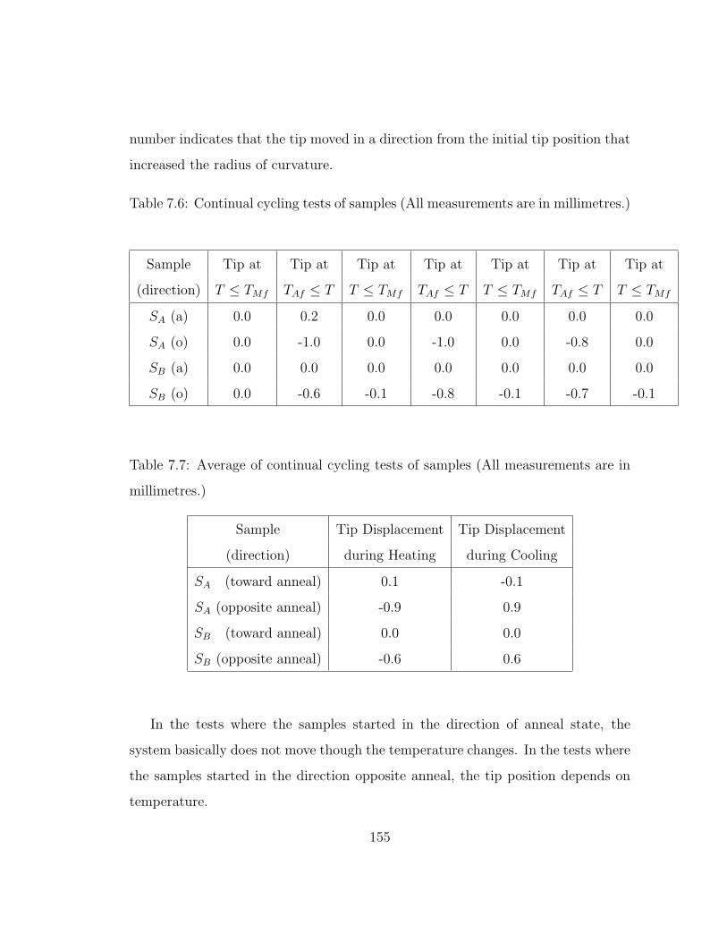
number indicates that the tip moved in a direction from the initial tip position that
increased the radius of curvature.
Table 7.6: Continual cycling tests of samples (All measurements are in millimetres.)
Sample Tip at Tip at Tip at Tip at Tip at Tip at Tip at
(direction) T ≤ TMf TAf ≤ T T ≤ TMf TAf ≤ T T ≤ TMf TAf ≤ T T ≤ TMf
SA (a) 0.0 0.2 0.0 0.0 0.0 0.0 0.0
SA (o) 0.0 -1.0 0.0 -1.0 0.0 -0.8 0.0
SB (a) 0.0 0.0 0.0 0.0 0.0 0.0 0.0
SB (o) 0.0 -0.6 -0.1 -0.8 -0.1 -0.7 -0.1
Table 7.7: Average of continual cycling tests of samples (All measurements are in
millimetres.)
Sample Tip Displacement Tip Displacement
(direction) during Heating during Cooling
SA (toward anneal) 0.1 -0.1
SA (opposite anneal) -0.9 0.9
SB (toward anneal) 0.0 0.0
SB (opposite anneal) -0.6 0.6
In the tests where the samples started in the direction of anneal state, the
system basically does not move though the temperature changes. In the tests where
the samples started in the direction opposite anneal, the tip position depends on
temperature.
155
7.1.3 Nature of Actuator Summary
The deformation and continual cycling tests performed on the actuators provide
information about the success of the local-annealing procedure. Since each sample
recovered its high-temperature shape after being deformed at low temperature in
the deformation test, it is clear that the actuator demonstrates the SME.
As the sample was cycled from high temperature to low temperature, the sample
did not move appreciably if it was initially deformed from its direction of anneal
state. It is speculated that this occurs because the buckled portal is not storing
adequate energy to deflect the martensite beam.
If the sample was initially in the direction opposite anneal state, the sample’s
shape changed from a high-temperature shape to a low-temperature shape. In this
case, the high-temperature shape can be described by a greater radius of curvature
than the low-temperature shape. There was movement in this state since the middle
beam was starting in the direction opposite anneal state. The middle beam was
manually deformed from its annealed shape. There was more strain stored in the
portal in this shape. When heated, the middle beam attempted to recover its
memorized position. When the heat was removed, the portal caused the middle
beam to return to the low-temperature equilibrium position.
7.2 Nature of Actuator’s Middle Beam
Quantitative tests were performed on the middle beam to understand the success
of the local annealing process. The deformation and continual cycling tests were
performed on the middle beam of SB once its girder was removed.
In the deformation test, the middle beam was manually deformed at T ≤ TMf .
156
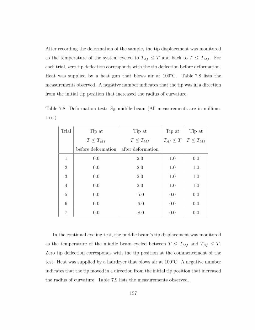
After recording the deformation of the sample, the tip displacement was monitored
as the temperature of the system cycled to TAf ≤ T and back to T ≤ TMf . For
each trial, zero tip deflection corresponds with the tip deflection before deformation.
Heat was supplied by a heat gun that blows air at 100C. Table 7.8 lists the
measurements observed. A negative number indicates that the tip was in a direction
from the initial tip position that increased the radius of curvature.
Table 7.8: Deformation test: SB middle beam (All measurements are in millime-
tres.)
Trial Tip at Tip at Tip at Tip at
T ≤ TMf T ≤ TMf TAf ≤ T T ≤ TMf
before deformation after deformation
1 0.0 2.0 1.0 0.0
2 0.0 2.0 1.0 1.0
3 0.0 2.0 1.0 1.0
4 0.0 2.0 1.0 1.0
5 0.0 -5.0 0.0 0.0
6 0.0 -6.0 0.0 0.0
7 0.0 -8.0 0.0 0.0
In the continual cycling test, the middle beam’s tip displacement was monitored
as the temperature of the middle beam cycled between T ≤ TMf and TAf ≤ T .
Zero tip deflection corresponds with the tip position at the commencement of the
test. Heat was supplied by a hairdryer that blows air at 100C. A negative number
indicates that the tip moved in a direction from the initial tip position that increased
the radius of curvature. Table 7.9 lists the measurements observed.
157

Table 7.9: Continual cycling test: SB middle beam (All measurements are in mil-
limetres.)
Sample Tip at Tip at Tip at Tip at Tip at Tip at Tip at
T ≤ TMf TAf ≤ T T ≤ TMf TAf ≤ T T ≤ TMf TAf ≤ T T ≤ TMf
SB 0.0 0.0 0.0 0.0 0.0 0.0 0.0
The deformation test shows that the middle beam exhibits the SME. Thus, the
annealing of the middle beam was successful. The continual cycling test indicates
that without the presence of the bias load the macroscopic shape of the middle
beam remains constant as the temperature cycles between T ≤ TMf and TAf ≤ T .
These tests indicate that the middle beam exhibits the expected behaviour of a
material that has the SME. However, these tests on the middle beam do not show
whether the portal was affected.
7.3 Nature of Actuator’s Portal
In the proposed design, the portal is the non-annealed part. This section seeks to
evaluate if the portal was affected by the heat treatment. The deformation and
continual cycling tests were attempted on the portal’s cantilever beams of SB once
the girder of SB was removed.
It was not possible to deform the portal’s cantilever beams. After removing an
external load that was intended to deform them at low temperature, the portal’s
beams sprung back to their initial shape. The “spring-like” behaviour of the beams
is not consistent with the behaviour of martensite.
158

In the continual cycling test, the portal’s cantilever beams were monitored as
the temperature of the beams cycled between T ≤ TMf and TAf ≤ T . The tips
vibrated due to the application of forced convection, but showed no net motion.
These tests indicate that the portal’s cantilever beams were not annealed.
7.4 Prototype Testing using Current
In the previous tests discussed in this chapter, heating of the samples was achieved
through forced convection of warm air. However, it is desired that prototype actua-
tion be achieved through electrical current. This section investigates using current
to actuate sample SC .
Sample SC was constrained in the fixture detailed in Chapter 6 and annealed
for two minutes. An input current of 23.7A was supplied to the Nichrome strip.
After the local-annealing process, the sample was placed in a vice so that its x-z
plane was parallel to gravity. Emery cloth was used to polish the sample’s surface
before attaching electrical leads to the fixed end and free end of the middle beam.
A thermocouple was welded to the sample at the mid-point of the middle beam
before the heat-treatment process. Figure 7.5 shows the experimental set-up from
a side view (left) and a top view (right).
The deformation test was used to determine if the sample responds to current.
In this test, the sample was manually deformed at T ≤ TMf . Zero tip deflection
corresponds with this initial tip deflection. The tip displacement was monitored
as current was first applied, and then removed. This test was performed three
times on SC . It was expected that after a sample is deformed it will return to the
high-temperature equilibrium position when TAf ≤ T and then move toward the
159

Figure 7.5: Prototype testing using current. Experimental set-up side view (left,
sample obscured by clips) and top view (right).
low-temperature equilibrium position when T ≤ TMf . Due to the buckling of the
portal’s cantilever beams and the mass of the electrical leads, it was not possible
to predict ytip.
Tables 7.10, 7.11, and 7.12 list the deformation tests measurements. In these
tables, the first row of measurements corresponds with the initial tip deflection of
the deformed sample at T ≤ TMf . The second row of measurements corresponds
with the tip deflection of the sample at TAf ≤ T while the last row of measurements
corresponds with the tip deflection of the sample at T ≤ TMf . A negative number
indicates that the tip was in a direction from the initial tip position that increased
the radius of curvature.
The results indicate that the sample recovered its high-temperature shape after
being deformed at low temperature. As the sample was then cycled from high
temperature to low temperature, it moved appreciably. Though a quantitative
comparison to simulated results is not possible, the amount of motion achieved
by the actuator is greater than expected, especially considering the mass of the
160

Table 7.10: First deformation test of SC
Tip Temperature Voltage Current
(mm) (C) (V) (A)
0.0 23 0.0 0.0
-4.5 74 1.0 3.4
-2.0 23 0.0 0.0
Table 7.11: Second deformation test of SC
Tip Temperature Voltage Current
(mm) (C) (V) (A)
0.0 23 0.0 0.0
-7.0 77 1.1 3.5
-6.0 23 0.0 0.0
Table 7.12: Third deformation test of SC
Tip Temperature Voltage Current
(mm) (C) (V) (A)
0.0 23 0.0 0.0
-8.0 74 1.1 3.5
-5.0 23 0.0 0.0
161
electrical lead at the free end of the middle beam and the attached thermocouple.
This series of tests confirms that the sample can be actuated through current.
Note that the current used in simulations is greater than the current needed
in these experiments. One possible reason why the currents differ may be because
the simulated current was extrapolated from data for Flexinol r©whereas the proto-
type was made with a SM495 strip from Nitinol Devices & Components. Another
possible reason is that the value for the convection heat transfer coefficient used
in simulation was not obtained experimentally, but taken from [18]. This esti-
mate for the convection heat transfer coefficient will affect the current-temperature
relationship in simulation.
7.5 Microstructure
Since the microstructure of martensite looks different than the microstructure of as-
rolled NiTi, investigating the microstructure of the middle beam and portal would
provide insight into the annealing procedure’s effectiveness. Since the previous
sections investigated the behaviour of the beams, this section focuses on the girder.
It is necessary to perform a metallographic sample preparation on the girder
to reveal the true sample structure. An excellent resource on procedures relating
to sample preparation is [56]. Due to the size of the actuator, it was necessary to
section it before proceeding with the sample preparation. A girder of an annealed
sample was removed and embedded in resin to examine its y-z plane at the inter-
section of the cantilevers with the girder. To embed the sample in the resin, a hot
compression mounting technique was used due to the availability of necessary ap-
paratus at the University of Waterloo and due to the relatively short process time.
Bakelite was the type of resin used. Bakelite requires that the sample be baked
162
under pressure for six minutes at 180C. After the sample was set, the material was
ground and polished. In these operations, abrasive particles are used to remove
material from the surface in successively finer steps.
After preparing the sample, it was examined under an optical microscope. Un-
fortunately, it was difficult to see the grain structure. This was because the surface
to be observed was no longer plane due to the pressure used to put the girder in the
resin. Correspondingly, cold mounting, another technique used to embed a sam-
ple in resin without the application of pressure, may have provided better results.
Also, using alumina to polish may not have been sufficient to remove damaged or
deformed surface material. Due to cost, the polishing cloths and polishing media
available in a general lab were used. To obtain a better sample, it would have been
better to determine the best type of polishing cloths and polishing media for NiTi.
On a macroscopic scale at a low temperature, an SMA is a conglomerate of
martensite plates [18]. These plates in NiTi are very fine, but are large enough to
be seen with an optical microscope in many other SMAs. The fineness of the plates
could be another reason why it was difficult to look at the grain structure.
Note that a comparison of the actuator’s phase at high temperature was not
attempted since it was not possible to keep the material at the required temperature
while doing the sample preparation.
7.6 Prototype Testing Summary
This chapter focused on the prototyping of two samples to determine if the shape-
set and heat-treatment process is successful. Results from tests performed on the
system, the middle beams, and the portal’s cantilever beams indicate that the
163

middle beam was successfully locally annealed. However, no information about
the nature of the girder was obtained. A series of tests performed on an additional
sample confirms that the prototype can be actuated through electrical current. It is
now necessary to compare the behaviour of the treated actuator with the expected
model behaviour.
164

Chapter 8
Discussion
After modelling and simulating the proposed actuator in Chapters 3 and 5, Chap-
ters 6 and 7 outlined prototype fabrication and testing. This chapter focuses on
comparing the simulated and experimental results, discussing differences between
the model and the actual system, and the method of obtaining measurements.
8.1 Result Comparison
Due to portal buckling, it is not possible to quantitatively compare the simulated
and experimental results. The simulated system and the prototypes are different.
Although a direct comparison is not possible, it is still possible to comment on the
results obtained.
The linear and non-linear simulated models indicate that the system’s temper-
ature increases as current is input into the actuator. This increase in temperature
causes the martensite phase fraction to decrease and the middle beam’s Young’s
modulus to increase. The corresponding increase in stiffness causes the actuator to
165

move toward the high-temperature equilibrium position. When power is not applied
to the system, the temperature decreases. This causes an increase in the marten-
site phase fraction. Consequently, the portal is able to move the annealed beam to
its low-temperature equilibrium position. The difference between the equilibrium
positions in simulation is 0.34mm [compare Figure 5.7].
The manufactured actuators had two states after annealing as a result of the
portal’s cantilever beams buckling. The movement of the actuators varies between
0mm and 1mm. The amount of movement depends on the initial state of the
actuator. The actuator does not move appreciably if it was initially deformed from
its direction of anneal state. If the sample was initially in the direction opposite
anneal state, the actuator’s tip moves by cycling the sample’s temperature. In this
state, the middle beam is manually deformed from its annealed shape. There is
more strain stored in the portal in this shape. When heated, the middle beam
attempts to recover its memorized position. When the heating is removed, the
portal restores the system to its low-temperature equilibrium position.
The deflections predicted by simulation and observed experimentally are in the
same order of magnitude. The theoretical and actual systems show that movement
can be obtained if adequate energy is stored in the portal. Attention must be paid
to the buckling of the portal’s cantilever beams that prevents the direct comparison
of systems.
8.2 Portal Buckling
The two states that are created by the buckling of the portal are due to the shrinkage
of the middle beam. It is hypothesized that the middle beam shortens due to the
release of residual cold-work.
166

The material supplied by Nitinol Devices & Components is as-rolled SM495
strip. The material is highly cold-worked and will not exhibit the shape memory
characteristics unless it is shape-set and some of that cold-work is removed. Before
heat treating the sample, it felt “springy” at low temperature. The cold-work
prevents the twinning deformation that makes the material feel “martensitic” [44].
Heat treating the middle beam relieves residual stresses. It is hypothesized that
the middle beam shortens as residual cold-work is relieved. This recovery exerts
a compressive force on the portal’s cantilever beams causing them to buckle. The
resulting configuration naturally has two stable states.
8.3 Differing Factors
Although it is difficult to compare the simulated and experimental results, it is
possible to comment on certain things that are different between the model and the
prototypes. These include dimensional differences and property values.
8.3.1 Dimensional Differences
The dimensions used in the model do not match the exact dimensions of the proto-
types. The widths, bb and bp, do not have the exact 2:1 ratio due to manufacturing
difficulties. When using waterjet technology to fabricate a small part like an ac-
tuator, the material provided should be bigger than the part width so that the
production of the part can be more accurately controlled. Since the width of the
provided material was set, an option was to make the actuator’s width smaller than
the width of the provided material. This option was discarded since making the
actuator’s width smaller increases difficulties in waterjet fabrication due to limita-
167
tions in fabrication accuracy. Conventional waterjet technology has an accuracy of
± 0.08mm [57]. Hence, the available material and the specified actuator geome-
try did not allow for any margin of extra material for positioning. The fact that
the portal’s width is not consistent affects the system as the middle beam heats.
It is expected that the portal’s cantilever beam with the greatest width pulls the
annealed beam toward itself.
8.3.2 Property Values
The material properties of a device affect its performance since these characteristics
help dictate response. Some of the properties used in simulation were not obtained
experimentally from the material used. Instead, they were taken from other sources
that provided information about values for typical NiTi. Also, some properties were
assumed constant when they are in fact functions of temperature. For instance,
although the resistivity of SMAs varies with temperature [33], it was assumed
constant in both models. Also, some property values for the annealed material
as martensite were used in simulation when property values of the non-annealed
material and annealed material as austenite were unavailable.
8.4 Obtaining Measurements
The prototypes’ displacements were obtained by magnifying each system and a
ruler with millimetre graduations. This is not a very precise method of obtaining
measurements. A high-precision three-dimensional computer vision tracking system
would provide greater accuracy. Also, it would be interesting to obtain real-time
measurements using current as an input so that the time response of the system
168
could be observed. Using current as the input instead of heated air prevents the
system from being influenced by forced convection.
8.5 Discussion Summary
Although it is desirable that a model be verified with results from different exper-
iments, it was not possible to use the prototypes to verify the simulations due to
the buckling of the portal’s cantilever beams. Once the challenge of residual stress
is rectified, simulations and experimental results should be compared in order to
ensure that the same result is achieved theoretically and experimentally.
169
Chapter 9
Conclusions
This research developed a scalable monolithic SMA actuator for potential incorpo-
ration in a robot for use in the digestive system. The use of local annealing is a
technique that can be used to fabricate a monolithic SMA actuator. In this type
of device, the annealed regions exhibit the SME while the remaining non-annealed
parts demonstrate elastic behaviour. Monolithic SMA actuators integrate the bias
force and reset mechanism within the same piece of material. The development of
this actuator requires developing a model for the system, simulating its behaviour,
prototyping the design, and comparing the experimental prototype behaviour with
the predicted model behaviour.
Since it is difficult to create a continuous model that exhibits the annealed
section’s ability to return to its memorized shape when heated, a lumped electro-
mechanical model is developed. The annealed and non-annealed sections are rep-
resented by a dynamic system that comprises equivalent springs and equivalent
masses for the annealed beam and the non-annealed portal. The equivalent spring
constant of the annealed section is a function of temperature. Two different models
170
are used to represent this dependence. The models are named the linear Young’s
modulus system model and the non-linear Young’s modulus system model.
To determine the validity of the lumped models, simulations were performed
based on the dimensions of a NiTi strip. The heating model for both the linear
and non-linear models are the same. When the current flows, the temperature
of the annealed beam increases. When the current ceases, the temperature of
the annealed beam decreases. The linear model does not directly calculate the
martensite phase fraction Rm. It implicitly assumes that Rm is linearly related
to T , meaning that at T ≤ TMf Rm = 1 and at T ≥ TAf Rm = 0. In the
non-linear model, the proximity of the temperature of the annealed beam to a
transformation temperature dictates the rate at which Rm changes. The non-linear
model incorporates the effects of hysteresis and minor loops. Correspondingly,
the linear model linearly changes the Young’s modulus for the annealed beam Eb
with respect to T while the non-linear model non-linearly changes Eb with respect
to T . Both models predict a tip displacement of 0.34mm if the middle beam
is fully transformed from one phase to another. When current is applied, the
system moves toward the high-temperature equilibrium position yb,h. When current
is not applied, the non-annealed portal acts as a bias spring to return the tip
toward the low-temperature equilibrium position yb,l. In the linear model, the
annealed beam begins moving at the appropriate transformation start temperature
and stops moving at the appropriate transformation finish temperature. However
in the non-linear model, the actuator tip moves before and beyond the start and
finish transformation temperatures respectively. The simulations indicate that the
annealed and non-annealed regions work together to achieve the desired motion.
Prototyping is necessary to determine a model’s validity. To determine the
actuator’s intended functionality, the proposed actuator was machined from a sin-
171
gle piece of non-annealed NiTi and then locally annealed so that the device has
temperature-active and temperature-passive sections. To assess the shape-set and
heat-treatment process, fabricated prototypes were tested. Results from tests per-
formed indicate that the middle beam was successfully annealed and that the por-
tal’s cantilever beams were not. However, no information about the nature of the
girder was obtained. A series of tests also confirmed that the device can be suc-
cessfully actuated through electrical current.
The next step was to compare the behaviour of the treated actuator with the
expected model behaviour. The deflections predicted by simulation and observed
experimentally are in the same order of magnitude. The theoretical and actual
systems show that movement can be obtained if adequate energy is stored in the
portal. However, attention must be paid to the buckling of the portal’s cantilever
beams that prevent the direct comparison of the systems. Once the challenge
causing the buckling is rectified, simulations and experimental results should be
compared in order to ensure that the same result is achieved theoretically and
experimentally.
This work has demonstrated the local annealing of a NiTi actuator and demon-
strated that the proposed design achieves movement. There is much promise in
this design and method of monolithic actuator fabrication. However, there remains
much work as well.
172
Chapter 10
Future Work
While the initial modelling and simulation work appears promising and useful, much
remains to be done. Assumptions made should be evaluated and improved. Opti-
misation of dimension selection and fabrication techniques would also improve the
actuator’s design. Investigation of the cyclic behaviour of the actuator would pro-
vide insights into its application. Other milestones in this long-term project include
integrating electronics and control, delivering power, and assessing the actuator’s
biomedical feasibility.
10.1 Assumption Improvements
Model development and simulation required assuming certain parameter values and
making model simplifications. Certain parameters were taken from sources that do
not detail how the parameters were obtained, such as htc. Other parameters, such
as ρe, csh, ρm, and Gm, were assumed constant as the material changed its phase.
Properties of materials assumed similar to NiTi SM495 strip were used when the
173
desired properties were not available for NiTi SM495 wire, including cm, kmC ,
kmH , and Em,d. Improvements to the Young’s modulus to stiffness model include
using relationships for a curved cantilever beam with an end-point load instead of
restraining the tip displacement to less than 7% of the beam’s length so that linear
elastic material and linear strain-displacement relationship analysis techniques can
be used. The heating model could be improved by incorporating a spatial thermal
distribution instead of assuming constant temperature throughout the actuator.
This more realistic approach would better identify what percentage of the material
has transformed. Accounting for external forces and other environmental factors,
such as pressures and liquids in the tract, would provide more information on the
actuator’s performance in its intended environment. These model enhancements
may enable the simulations to better match the prototype’s behaviour.
When using finite element analysis to design the fixture, the actuator’s surface in
contact with the Nichrome was set at 500C. This temperature was time-invariant
and constant along the surface. In reality, the Nichrome supplies a certain amount
of energy to the system, not a fixed temperature. Since the time to heat the
middle beam’s surface is unknown, this assumption requires investigation. The
finite element model could also have incorporated the resistive heating element so
that the conduction between the parts would have been taken into account when
designing the dies’ heights.
10.2 Dimension Selection
The chosen prototype dimensions were based on the dimensions of a supplied NiTi
strip. The design was not dimensionally optimised. There is a more effective
thickness-to-width ratio that could be determined by constraining the maximum
174
tensile stress at high temperature and strain at low temperature to values that
ensure that the required fatigue life is obtained [31]. Also, bb and bAB were chosen
arbitrarily in the ratio 2:1. Varying this ratio and observing the results could lead
to a better result.
Modifying the dimensions affects the ease of buckling. Whether a column will
buckle depends on the material’s Young’s modulus and the column’s dimensions,
particularly its length and its moment of inertia [8]. It is important to note that
a column will buckle about the principal axis of the cross-section having the least
moment of inertia [8]. Since the least moment of inertia for the portal’s cantilever
beams is about the z-axis, increasing the prototype’s thickness would increase the
least moment of inertia thus reducing the ease of buckling.
10.3 Fabrication Techniques
Instead of locally annealing NiTi with an electrically heated strip of Nichrome in
a fixture, the use of direct Joule heating or a laser should be investigated. In
direct Joule heating, the material is heated up to its annealing temperature using
a direct current. One possible idea to locally anneal the proposed prototype using
direct Joule heating is to supply current to the mid-point of the middle beam while
grounding the fixed and free ends of the middle beam [58]. According to [33], laser
annealing is a flexible, contactless, and cheap technology that is more promising
than direct Joule heating. Hence, its use should also be examined.
The manufactured actuators had two states after annealing due to the buckling
of the portal’s cantilever beams. It is hypothesized that the buckling of the portal’s
beams is related to the shortening of the middle beam that occurs as a result of
the release of residual cold-work. This residual stress may have been introduced
175
during the rolling stage of fabrication, the coiled storage position, or the waterjet
fabrication process. Had the fixture constrained the middle beam in all dimensions,
buckling may not have occurred. It is important to determine the cause of the
buckling and modify the fabrication techniques to prevent it if possible.
10.4 Cyclic Behaviour
To understand the behaviour of the actuator over time, it is critical to cycle NiTi
between fixed strain amplitudes for a specified number of cycles or until failure.
While cycling, it is possible to test if heating and cooling occur within the desired
time period.
10.5 Other Milestones
Other milestones in this long-term project include integrating electronics and con-
trol, delivering power, and assessing the actuator’s biomedical feasibility.
If the actuator is integrated in a robot for use in the digestive tract, future
efforts will target the inclusion of electronics and control circuitry on the device to
enable gait.
Supplying adequate power to the device is essential. Although the present model
assumes resistive heating through current presumably delivered from miniature
batteries or a miniature power plant on the robot, there are other possibilities.
Power requirements could be supplied by an on-board capacitor that is charged
with electric power transmitted wirelessly from an external control unit [16]. The
176

prospect of using magnetically-actuated SMAs should also be considered in future
work.
It is important to know the effect of the actuator on its environment. The gut
is a highly flexible and slippery environment. It is also very fragile and sensitive
to damage [11]. To gain a basic understanding, sections of the human intestine
tract can be built using bovine or pig intestines. This will demonstrate whether the
mechanism is too intrusive. If this is the case, perhaps another actuator with a more
“worm-like” behaviour could be developed using local annealing of a monolithic
piece of NiTi.
10.6 Future Work Summary
This thesis focused on the model development, simulation, and prototyping of a
locally-annealed monolithic SMA actuator. It is an initial work actualized to es-
tablish the feasibility of the actuator. Although this project continues to present
many challenges, the preliminary results are encouraging.
177
Bibliography
[1] American College of Gastroenterology, “Patient information.” [Online]. Avail-
able: http://www.acg.gi.org/patientinfo/cgp/index.html, August 2003 [date
accessed].
[2] P. Dario, B. Hannaford, and A. Menciassi, “Smart surgical tools and augment-
ing devices,” IEEE Transactions on Robotics and Automation, vol. 19, no. 5,
2003.
[3] Astra Pharmaceuticals, “An introduction to GERD.” [Online]. Available:
http://www.gerd.com/intro/frame/frame.htm, August 2003 [date accessed].
[4] Given Imaging Ltd., “Patients.” [Online]. Available:
http://www.givenimaging.com/Cultures/en-US/Given/english/Patients/,
August 2003 [date accessed].
[5] Three Rivers Endoscopy Center, “Wireless capsule endoscopy: The camera in
a pill.” [Online]. Available: http://www.gihealth.com/html/test/given.html,
August 2003 [date accessed].
[6] U.S. Food and Drug Administration, “Given diagnos-
tic imaging system - K010312.” [Online]. Available:
178

http://www.fda.gov/cdrh/mda/docs/k010312.html, August 2003 [date
accessed].
[7] F. Incropera and D. DeWitt, Fundamentals of Heat and Mass Transfer. New
York, New York: John Wiley & Sons, 4th ed., 1996.
[8] R. Hibbeler, Mechanics of Materials. Englewood Cliffs, New Jersey: Prentice
Hall, Inc., 3rd ed., 1997.
[9] M. Farabee, “Online biology book glossary.” [Online]. Available:
http://www.emc.maricopa.edu/faculty/farabee/BIOBK/digest.gif, March
2003 [date accessed].
[10] A. Gutyton and J. Hall, Textbook of Medical Physiology. Philadelphia, Penn-
sylvania: W.B. Saunders Company, 9th ed., 1996.
[11] D. Reynaerts, J. Peirs, and H. V. Brussel, “Shape memory micro-actuation for
a gastro-intestinal intervention system,” Sensors and Actuators A: Physical,
vol. 77, pp. 157–166, October 1999.
[12] H. Gray, P. L. Williams, and L. H. Bannister, Gray’s Anatomy: The Anatom-
ical Basis of Medicine and Surgery. Edinburgh, Scotland: Churchill Living-
stone, 38th ed., 1995.
[13] R. H. Sturges and S. Laowattana, “A flexible, tendon-controlled device for
endoscopy,” International Journal of Robotics Research, vol. 12, pp. 121–131,
1993.
[14] J. Van Dam and W. R. Brugge, “Endoscopy of the upper gastrointestinal
tract,” The New England Journal of Medicine, vol. 341, pp. 1738–1748, De-
cember 1999.
179
[15] C. Becker, “And now, live from your lower intestine...,” Modern Healthcare,
vol. 33, pp. 50–52, February 2003.
[16] RF SYSTEMlab, “NORIKA3.” [Online]. Available:
http://www.rfnorika.com/, June 2004 [date accessed].
[17] E. Amatucci, N. Dagalakis, B. Damazo, M. Davies, J. Evans, and J. Song, “An
overview of nano-micro-meso scale manufacturing at the National Institute of
Standards and Technology,” in Proceedings of the Nano Tribology Workshop,
(Gaithersburg, Maryland), March 2000.
[18] D. R. Madill, “Modelling and stability of a shape memory alloy position con-
trol system,” Master’s of Applied Science, University of Waterloo, Waterloo,
Ontario, 1993.
[19] A. Teshigahara, M. Watanabe, N. Kawahara, I. Ohtsuka, and T. Hattori, “Per-
formance of a 7-mm microfabricated car,” Journal of Microelectromechanical
Systems, vol. 4, pp. 76–80, June 1995.
[20] F. F. Ling, E. F. Gloyna, and J. Stellato, “Visit to
DENSO Research Laboratories and first international sympo-
sium on laser precision microfabrication.” [Online]. Available:
http://www.arofe.army.mil/Reports/Mechanical/denso report.htm, July
2000 [date accessed].
[21] H. Choi, S. Ryew, K. Jung, H. Kim, J. Jeon, J. Nam, R. Maeda, and
K. Tanie, “Soft actuator for robotic applications based on dielectric elastomer:
Quasi-static analysis,” in Proceedings of the IEEE International Conference
on Robotics and Automation, vol. 3, (Washington, D.C.), pp. 3217–3217, May
2002.
180

[22] V. Varma and W. Dixon, “Design of a piezoelectric meso-scale mobile robot: A
compliant amplification approach,” in Proceedings of the IEEE International
Conference on Robotics and Automation, vol. 2, (Washington, DC), pp. 1137–
1142, May 2002.
[23] Q. Chen, D.-J. Yao, C.-J. Kim, and G. P. Carman, “Mesoscale actuator device:
Micro interlocking mechanism to transfer macro load,” Sensors and Actuators
A: Physical, vol. 73, pp. 30–36, March 1999.
[24] C. Cabuz, W. R. Herb, E. I. Cabuz, and S. T. Lu, “The dual diaphragm
pump,” in Proceedings of the IEEE International Conference on Micro Electro
Mechanical Systems, pp. 519–522, January 2001.
[25] Unknown, “Micropumps review.” [Online]. Available:
http://home.cwru.edu/∼bxl24/Archive/Micropumps%20Review.pdf, Septem-
ber 2004 [date accessed].
[26] J. Peirs, D. Reynaerts, and H. Van Brussel, “Shape memory micro-actuators
for medical purposes,” in Proceedings of the International Conference on Ad-
vanced Robotics, pp. 155–160, 1997.
[27] Johnson Matthey, Inc., “Nitinol technical data\application notes.” [Online].
Available: http://www.jmmedical.com/html/resource library.html, July 2004
[date accessed].
[28] A. Pelton, J. DiCello, and S. Miyazaki, “Optimisation of processing and prop-
erties of medical grade Nitinol wire,” in Minimally Invasive Therapy and Allied
Technologies, vol. 9, pp. 107–118, 2000.
[29] T. Duerig, K. Melton, D. Stockel, and C. Wayman, eds., Engineering Aspects
of Shape Memory Alloys. Butterworth-Heinemann, 1990.
181
[30] S. M. Russell, “Nitinol melting and fabrication,” in Proceedings of the Interna-
tional Conference on Shape Memory and Superelastic Technologies (S. Russell
and A. Pelton, eds.), (Asilomar, California), 2000.
[31] T. Waram, Actuator Design using Shape Memory Alloys. Hamilton, Ontario:
T.C. Waram, 2nd ed., 1993.
[32] B. F. Keats, “Temperature compensation for cavity resonators using shape
memory alloys,” Master of Applied Science, University of Waterloo, Waterloo,
Ontario, 2003.
[33] Y. Bellouard, T. Lehnert, J.-E. Bidaux, T. Sidler, R. Clavel, and R. Got-
thardt, “Local annealing of complex mechanical devices: A new approach for
developing monolithic micro-devices,” Materials Science and Engineering A:
Structural Materials: Properties, Microstructure and Processing, vol. A273-
275, pp. 795–798, 1999.
[34] R. Gorbet, D. Wang, and K. Morris, “Preisach model identification of a two-
wire SMA actuator,” in Proceedings of the IEEE International Conference on
Robotics and Automation, vol. 3, pp. 2161–2167, 1998.
[35] Y. Haga and M. Esashi, “Biomedical microsystems for minimally invasive di-
agnosis and treatment,” Proceedings of the IEEE, vol. 92, no. 1, pp. 98–114,
2004.
[36] Y. Haga, T. Mineta, and M. Esashi, “Active catheter, active guide wire and
related sensor systems,” in Proceedings of the 5th Biannual World Automation
Congress, vol. 14, pp. 291–296, 2002.
[37] P. Dario, M. Carrozza, L. Lencioni, B. Magnani, and S. D’Attanasio, “A mi-
crorobotic system for colonoscopy,” in Proceedings of the IEEE International
182

Conference on Robotics and Automation, vol. 2, (Albuquerque, New Mexico),
pp. 1567–1572, April 1997.
[38] D. J. Inman, Engineering Vibration. Englewood Cliffs, New Jersey: Prentice
Hall, Inc., 1994.
[39] J. Shigley and C. Mischke, Mechanical Engineering Design. New York, New
York: McGraw-Hill Book Company, Inc., 5th ed., 1989.
[40] K. Ikuta, M. Tsukamoto, and S. Hirose, “Mathematical model and exper-
imental verification of shape memory alloy for designing micro actuator,” in
Proceedings of the IEEE Micro Electro Mechanical Systems, pp. 103–108, 1991.
[41] S. Timoshenko and J. N. Goodier, Theory of Elasticity. New York, New York:
McGraw-Hill Book Company, Inc., 3rd ed., 1970.
[42] J. P. Den Hartog, Advanced Strength of Materials. New York, New York:
McGraw-Hill Book Company, Inc., 1952.
[43] Nitinol Devices & Components, “Nitinol SM495 wire.” [Online]. Avail-
able: http://www.dsl-online.de/ndc2/pdf files/sm495 wire data.pdf, July
2004 [date accessed].
[44] M. Boyle (Employee of Nitinol Devices & Components), [Private electronic
communication]. January 2003.
[45] The MathWorks, “Simulink r© 6.” [Online]. Available:
http://www.mathworks.com/products/simulink/, July 2004 [date accessed].
[46] Dynalloy, Inc., “Flexinol r© technical data.” [Online]. Available:
http://www.dynalloy.com/TechnicalData.html, July 2004 [date accessed].
183
[47] COMSOL, Inc., “FEMLAB r© 3.0.” [Online]. Available:
http://www.comsol.com/products/femlab/, August 2004 [date accessed].
[48] Nitinol Devices & Components, “Nitinol facts.” [Online]. Available:
http://www.dsl-online.de/ndc2/pdf files/nitinol facts.pdf, April 2004 [date ac-
cessed].
[49] D.L. Williamson, J.A. Davis, and P.J. Wilbur, “Effect of austenitic stainless
steel composition on low-energy, high-flux, nitrogen ion beam processing,” Sur-
face & Coatings Technology, vol. 103-104, pp. 178–184, May 1998.
[50] F. A. Lowenheim, Electroplating. New York, New York: McGraw-Hill Book
Company, Inc., 1978.
[51] D. Allen, “Argument for consistency heats up sealing process.” [Online]. Avail-
able: http://www.devicelink.com/pmpn/archive/02/06/002.html, April 2004
[date accessed].
[52] A. Smith (PhD Candidate at the University of Waterloo), [Private communi-
cation]. 2004.
[53] Proscience, Inc., “MACOR r© Machinable Glass Ceramic.” February 2004.
[54] DuPontTM, “Kapton r© polymide film.” [Online]. Available:
http://www.dupont.com/kapton/, April 2004 [date accessed].
[55] MatWeb, “Material property data.” [Online]. Available:
http://matweb.com/index.asp?ckck=1, April 2004 [date accessed].
[56] Struers, “E-Metalog.” [Online]. Available: http://www.struers.com, July 2004
[date accessed].
184

[57] Baumeier Waterjet Technoloy, Inc., “Capabilities.” [Online]. Avail-
able: http://www.baumeierwaterjet.com/Capabilities/capabilities.html, Au-
gust 2004 [date accessed].
[58] K. Krauel (Lab Director for Systems Design Engineering at the University of
Waterloo), [Seminar]. July 2004.
185

List of Nomenclature
The units of the variables given in this list of nomenclature are possible units.
At times in the thesis, different scaling factors are used for the same variable (for
example, length in mm or m). The unit being used will be obvious from the context.
Ab surface area of annealed beam, m2
a horizontal distance in Figure 4.4, m
b vertical distance in Figure 4.4, m
bAB width of non-annealed portal’s cantilever beam, m
bb width of annealed beam, m
bBC width of non-annealed portal’s girder, m
bx damping coefficient (replace x with 1 and 2 in Figure 3.3), Nsm
cm reciprocal of the stress rate constant,CPa
csh specific heat, JkgK
d(b) tip displacement of cantilever in Figure 2.15 (b), m
d(c) tip displacement of cantilever in Figure 2.15 (c), m
d(d) tip displacement of cantilever in Figure 2.15 (d), m
dh deflection of spring at high temperature in Figure 2.16, m
dl deflection of spring at low temperature in Figure 2.16, m
Ea Young’s modulus of austenite, GPa
186
Eb Young’s modulus of annealed beam, GPa
Egen energy generated in a differential control surface, J
Ein energy entering through a differential control surface, J
Em Young’s modulus of martensite, GPa
Em,d Young’s modulus of martensite detwinned, GPa
Em,l Young’s modulus of martensite linear, GPa
Em,t Young’s modulus of martensite twinned, GPa
Eout energy leaving through a differential control surface, J
Ep Young’s modulus of as-rolled, GPa
Est energy stored in a differential control surface, J
F load, N
g gravity, ms2
Gm modulus of rigidity, GPa
htc convection heat transfer coefficient, Wm2K
I input current, A
IAB second moment of area of portal’s cantilever beam, m4
Ib second moment of area of annealed beam, m4
IBC second moment of area of girder, m4
Ix moment of inertia about the axis of rotation, m4kg
K kinetic energy (subscripts refer to different types of kinetic energy), W
k thermal conductivity, WmK
kb equivalent stiffness of annealed beam, Nm
kb,h equivalent stiffness of annealed beam at TAf ,Nm
kb,l equivalent stiffness of annealed beam at TMf ,Nm
km temperature constant (superscripts C and H correspond to cooling and
heating respectively), 1K
187

kp equivalent stiffness of portal, Nm
kx spring constant (replace x with 1 and 2 in Figure 3.3), Nm
LAB length of non-annealed cantilever beam, m
Lb length of annealed beam, m
LBC girder length, m
M moment, Nm
m mass, kg
mb equivalent mass of annealed beam, kg
mcant mass of portal’s cantilever beam, kg
Mint internal moment, Nm
mp equivalent mass of portal, kg
mx mass (replace x with 1 and 2 in Figure 3.3), kg
P load, N
Pe electrical input power, W
Qcond” conductive heat flux per unit area, Wm2
Qconv” convection heat flux per unit area, Wm2
Qrad” radiative heat flux per unit area, Wm2
R radius of curvature in Figure 4.4, m
Ra austenite phase fraction
Rm martensite phase fraction (superscripts C and H correspond to cooling and
heating respectively)
Rma hysteresis gain constant (superscripts C and H correspond to cooling and
heating respectively)
Rma0 initial hysteresis gain constant
Rmb hysteresis offset constant (superscripts C and H correspond to cooling and
heating respectively)
188

Rmb0 initial hysteresis offset constant
T temperature of annealed beam, K
t time, s
tAB thickness of non-annealed portal’s cantilever beam, m
TAf austenite finish temperature, K
Tanneal SMA annealing temperature, K
TAs austenite start temperature, K
tb thickness of annealed beam, m
tBC thickness of non-annealed portal’s girder, m
TMf martensite finish temperature, K
TMs martensite start temperature, K
Tr transformation temperature, K
ts switching time (superscripts 1 and 2 correspond to first and
second switching time respectively), s
T0 initial temperature of annealed beam, K
T0m average transformation temperature, K
T∆ temperature difference between T and T∞, K
T∆P temperature difference between T and T∞ from the previous time step, K
T∞ ambient temperature, K
Vb volume of middle beam, m3
yAB deflection of portal’s cantilever beam
(if subscript max then deflection is at the free end), m
yb deflection of annealed beam, m
yBC deflection of simply-supported beam with mid-beam load
(if subscript max then deflection is at mid-length), m
yb,h deflection of annealed beam at TAf , m
189

yb,l deflection of annealed beam at TMf , m
yb,max maximum deflection of annealed beam, m
yF tip deflection due to load F , m
yF/2 tip deflection due to load F/2, m
yflat deflection from curved position to flat position, m
yM tip deflection due to moment M , m
yp,max maximum deflection of non-annealed portal, m
ytip total tip deflection of annealed beam, m
β width-to-thickness proportionality constant
βC cooling proportionality constant, K
βH heating proportionality constant, K
∆F net force in Figure 2.18, N
∆t time step size, s
∆x displacement difference in Figures 2.17 and 2.18, m
ε strain, mm
εa strain of annealed beam when austenite, %
εm strain of annealed beam when martensite, %
εmd martensite detwin strain, m
m
εmy martensite twin strain, m
m
εs surface emissivity
θ angle of circle segment in Figure 4.4, rad
θBC,max maximum rotation of portal’s cantilever beam, rad
κ empirical constant
ρe electrical resistivity, Ωm
ρm density, kgm3
σ stress, Pa
190
σa stress if beam were completely austenite, Pa
σbend bending stress, Pa
σm stress if beam were completely martensite, Pa
σSB Stefan-Botzmann constant, Wm2K4
φ twist for cantilevers AB and DC, rad
ω angular velocity, rads
191

List of Acronyms and Chemical
Formulas
ANTLA antagonistically-driven linear actuator
CT computerised tomography
CuAlNi copper aluminium nickel
CuSO4 · 5H20 copper sulfate pentahydrate
CuZnAl copper zinc aluminium
DDP dual-diaphragm pump
EDM electrical discharge machining
FEA finite element analysis
GERD gastroesophageal reflux disease
GI gastrointestinal
H2SO4 sulfuric acid
IBD inflammatory bowel disease
MRI magnetic resonance imaging
Ni76Cr21A3 Nichrome [49]
NiTi nickel titanium
SMA shape memory alloy
SME shape memory effect
192