the development of a fluorescence-based reverse flow

University of South FloridaScholar Commons

Graduate Theses and Dissertations Graduate School

11-5-2015

The Development of a Fluorescence-based ReverseFlow Injection Analysis (rFIA) Method forQuantifying Ammonium at NanomolarConcentrations in Oligotrophic SeawaterWilliam AbbottUniversity of South Florida, [email protected]

Follow this and additional works at: http://scholarcommons.usf.edu/etd

Part of the Aquaculture and Fisheries Commons, Ocean Engineering Commons, and the OtherOceanography and Atmospheric Sciences and Meteorology Commons

This Thesis is brought to you for free and open access by the Graduate School at Scholar Commons. It has been accepted for inclusion in GraduateTheses and Dissertations by an authorized administrator of Scholar Commons. For more information, please contact [email protected].

Scholar Commons CitationAbbott, William, "The Development of a Fluorescence-based Reverse Flow Injection Analysis (rFIA) Method for QuantifyingAmmonium at Nanomolar Concentrations in Oligotrophic Seawater" (2015). Graduate Theses and Dissertations.http://scholarcommons.usf.edu/etd/5892

http://scholarcommons.usf.edu/?utm_source=scholarcommons.usf.edu%2Fetd%2F5892&utm_medium=PDF&utm_campaign=PDFCoverPages

http://scholarcommons.usf.edu/?utm_source=scholarcommons.usf.edu%2Fetd%2F5892&utm_medium=PDF&utm_campaign=PDFCoverPages

http://scholarcommons.usf.edu?utm_source=scholarcommons.usf.edu%2Fetd%2F5892&utm_medium=PDF&utm_campaign=PDFCoverPages

http://scholarcommons.usf.edu/etd?utm_source=scholarcommons.usf.edu%2Fetd%2F5892&utm_medium=PDF&utm_campaign=PDFCoverPages

http://scholarcommons.usf.edu/grad?utm_source=scholarcommons.usf.edu%2Fetd%2F5892&utm_medium=PDF&utm_campaign=PDFCoverPages

http://scholarcommons.usf.edu/etd?utm_source=scholarcommons.usf.edu%2Fetd%2F5892&utm_medium=PDF&utm_campaign=PDFCoverPages

http://network.bepress.com/hgg/discipline/78?utm_source=scholarcommons.usf.edu%2Fetd%2F5892&utm_medium=PDF&utm_campaign=PDFCoverPages




mailto:[email protected]

The Development of a Fluorescence-based Reverse Flow Injection Analysis (rFIA) Method for

Quantifying Ammonium at Nanomolar Concentrations in Oligotrophic Seawater

by

William R. T. Abbott

A thesis submitted in partial fulfillment

of the requirements for degree of

Master of Science

College of Marine Science

University of South Florida

Co-Major Professor: Kristen Buck, Ph. D.

Co-Major Professor: Kent Fanning, Ph. D.

Robert Masserini, Ph. D.

Jacqueline Dixon, Ph. D.

Date of Approval:

November 4, 2015

Keywords: Ammonia, Formaldehyde, Marine Environment, Nutrients, o-Phthaldialdehyde,

Sulfite

Copyright © 2015, William R. T. Abbott

i

Table of Contents

List of Tables ................................................................................................................................. iii

List of Figures ................................................................................................................................ iv

Abstract ............................................................................................................................................v

Chapter 1: Introduction and Objectives ...........................................................................................1

1. Ammonium Analysis .......................................................................................................5

2. Reverse Flow Injection Analysis ...................................................................................10

3. Objectives ......................................................................................................................11

Chapter 2: A Reverse Flow Injection Analysis Technique for the Fluorometric

Determination of Nanomolar Ammonium Concentrations in Seawater ..................................12

1. Background Information ................................................................................................12

2. Materials and Methods ...................................................................................................15

2.1 Reagents ...........................................................................................................15

2.1.1 rFIA Reagents ...................................................................................15

2.1.2 Standards ...........................................................................................16

2.1.3 Interference Solutes ..........................................................................16

2.1.4 GD-FIA Reagents .............................................................................17

2.2 Manifold Description .......................................................................................17

2.2.1 rFIA Experimental Manifold ............................................................18

2.2.2 GD-FIA Control Manifold ................................................................19

2.3 Procedure .........................................................................................................20

3. Results for the rFIA Ammonium Method ......................................................................22

3.1 Reaction Conditions .........................................................................................22

3.2 Reagent Blanks and Matrix Effects .................................................................24

3.3 Calibration Curve and Standard Additions ......................................................25

3.4 Amine and Amino Acid Interference ...............................................................26

4. Discussion ......................................................................................................................28

4.1 Temperature and OPA Concentration ..............................................................29

4.2 Background Fluorescence ................................................................................30

4.3 Blanks and Matrix Effects ...............................................................................31

4.4 Limit of Detection ............................................................................................31

4.5 Potential Interferences .....................................................................................32

5. Conclusions ....................................................................................................................33

6. Acknowledgments..........................................................................................................34

ii

Chapter 3: Conclusion....................................................................................................................35

References ......................................................................................................................................38

Appendix A ....................................................................................................................................42

iii

List of Tables

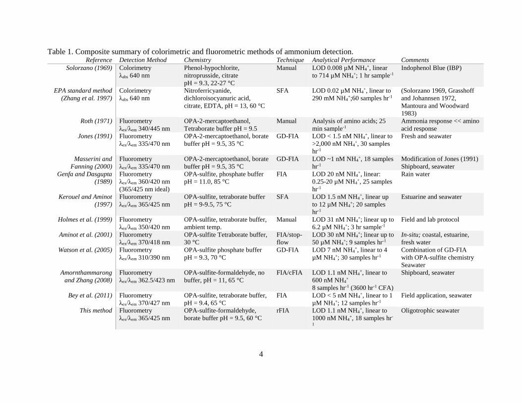
Table 1: Composite summary of colorimetric and fluorometric methods of ammonium

detection. ....................................................................................................................................4

Table 2: Potential interference from primary amines and amino acids. ....................................28

Table A1: Summary of calibration curve results. .........................................................................42

iv

List of Figures

Figure 1: rFIA background fluorescence. ....................................................................................14

Figure 2: rFIA and control (GD-FIA) manifold ..........................................................................18

Figure 3: Universal Data Collection calibration curve display ...................................................21

Figure 4: Slope variation with respect to temperature and OPA concentration. .........................23

Figure 5: Effect of salinity on calibration curve slope. ...............................................................25

Figure 6: Comparison of OPA techniques...................................................................................27

Figure 7: High resolution analysis. ..............................................................................................28

v

Abstract

The goal of this thesis was to adopt a reverse flow injection analysis (rFIA) technique to

the fluorometric analysis of the reaction o-phthaldialdehyde (OPA) with ammonium, allowing

accurate measurements of ammonium concentrations lower than the detection limit of the widely

used indophenol blue (IPB) colorimetric method while accounting for the background

fluorescence of seawater. Ammonium is considered an essential nutrient for primary

productivity, especially in the nutrient depleted surface ocean where as the most reduced form of

dissolved inorganic nitrogen, it is readily assimilated via metabolic pathways. Challenges in the

quantification of ammonium require more sensitive analytical techniques for a greater

understanding of the biogeochemical cycling of ammonium in the oligotrophic ocean. On-line

and automated flow analysis techniques are capable of mitigating some of the challenges.

Fluorescent-based methods out-perform colorimetric methods in terms of detection limits and

sensitivity. Presented here is the development of an rFIA technique paired with an OPA-sulfite

chemistry. For this method, a sulfite-formaldehyde reagent is mixed with the sample stream and

then injected with the OPA reagent before being heated. Fluorescence is measured before and at

the peak of the OPA injection, differentiating the background fluorescence from the analyte

signal. Experiments to optimize reaction parameters and characterize the effects of salinity and

potentially interfering species were conducted. The newly developed method offers a reasonable

throughput (18 samples per hour), low limit of detection (1.1 nM) ammonium analysis technique

with automatic background fluorescence correction suitable for oligotrophic seawater as a

preferable alternative to the low sensitivity and high limit of detection IPB colorimetric method.

1

Chapter 1: Introduction and Objectives

The open ocean accounts for 90% of the ocean surface area while coastal zones and

upwelling areas make up the remaining 9.9 and 0.1%, respectively (Schlesinger 2007). A

distinguishing feature of the open ocean is the limitation of primary productivity in the euphotic

zone by nutrient availability, frequently by nitrogen (Redfield et al. 1963). Fixed nitrogen is an

essential nutrient for the formation of DNA, amino acids, and proteins. Of the inorganic forms of

fixed nitrogen, ammonium is the most reduced and is readily assimilated into phytoplankton

(Dortch 1990, Pilson 1998), leading to a depletion of the nutrient in surface waters when not

replenished by autochthonous processes, N-fixation, atmospheric deposition, remineralization

and photo-oxidation of dissolved organic matter, or by other allochthonous input from terrestrial

sources or subsurface upwelling (Menzel and Spaeth 1962, Bushaw et al. 1996, Johnson et al.

2007, Schlesinger 2007, Johnson et al. 2008). Nitrogen, and specifically ammonium (NH4+),

availability in the oligotrophic surface ocean is not widely measured due to the inherent

challenges of these measurements. Improved measurement techniques as offered by the reverse

flow injection analysis method presented here can enhance the understanding of the

biogeochemical cycling of nitrogen that affects such a large portion of the ocean and its

ecosystems (Harrison et al. 1996, Schlitzer et al. 2003, Johnson et al. 2007, Johnson et al. 2008).

Ammonium concentrations in the oligotrophic ocean are difficult to characterize due to

sampling infrequency, analytical insensitivity of traditional measuring techniques, and the

complications of the seawater matrix on analytical techniques (Šraj et al. 2014). The wide variety

2

of ammonium analysis tools available has resulted in a recent publication of a guide to assist in

the selection of a method for determining ammonium in different types of waters and diverse

applications from industrial waste to drinking water and environmental monitoring (Molins-

Legua et al. 2006). In oceanic applications, a colorimetric method based on the Berthelot

reaction of ammonium with phenol-hypochlorite, forming indophenol blue (IPB) product, is

most frequently used and has been modified for automated segmented flow spectrophotometric

analysis (SFA) (Solorzano 1969, Grasshoff and Johannsen 1972, Mantoura and Woodward 1983,

Kerouel and Aminot 1997). Other methods (Nessler, indothymol, ion selective electrodes, solid

phase extraction) have sensitivities and ranges suitable for ammonium measurement in other

applications (Molins-Legua et al. 2006). The IPB method is suitable for coastal and estuarine

applications (with consideration given to matrix effects), where ammonium concentrations can

be in the micromolar range, but it suffers from poor interlaboratory comparisons at low

concentrations (e.g. 56% relative standard deviation for a 0.34 µM sample reported from a

survey of 106 marine labs conducted by Aminot et al. (1997)) and an insufficiently low limit of

detection (LOD between .004 and 1.4 µM NH4+ (Šraj et al. 2014)) for seawater applications.

Increasingly, the fluorogenic reaction of o-phthaldialdehyde (OPA) with ammonium has been

explored in manual and automated systems for measurement of nanomolar ammonium

concentrations, as fluorometry can offer a 10- to 100-fold increase in sensitivity relative to

spectrophotometric methods. (Table 1) (Roth 1971, Genfa and Dasgupta 1989, Jones 1991,

Kerouel and Aminot 1997, Holmes et al. 1999, Masserini and Fanning 2000, Aminot et al. 2001,

Watson et al. 2005, Frank and Schroeder 2007, Amornthammarong and Zhang 2008, Bey et al.

2011, Ma et al. 2014). However, natural fluorescence of dissolved organic matter and the

3

reaction of OPA with primary amines and amino acids creates analytical challenges for

fluorescent OPA detection of ammonium (Roth 1971, Masserini and Fanning 2000).

In addition to these analytical challenges for measuring the nanomolar ammonium

concentration in surface seawater, ammonium contamination of samples also complicates

measurements. Handling and preparation of reagents and ammonium samples exposes the

samples to sources of errors including atmospheric contamination, sample bottle surface

adhesion of ammonium, and uptake or release of ammonium during sample storage. Ammonium

is particularly difficult to measure due to its propensity to adsorb onto glass and plastic surfaces

and its high solubility in water (0.515 g NH4+ g-1 of water at 20 °C compared to 0.00172 g

CO2 g-1 water for carbon dioxide solubility (Van Der Linden 1983, Kerouel and Aminot 1997)).

Volatile nitrogenous compounds present in laboratory environments or as part of the reagents for

the analysis of other nutrients are common concerns among ammonium analysts (Aminot et al.

1997). Additionally, ammonium samples are subject to continued microbial utilization after

collection and should ideally be analyzed within 3 hours of collection, or within 1 week if frozen

(Zhang et al. 1997). Analysis of samples in automated systems, on-line or in-situ, bypasses many

of these sources of error in the handling process. Therefore, automated flow analysis techniques

paired with fluorometry offer the advantages of higher precision, lower contamination risk, lower

detection limits, and higher sample throughput relative to manual techniques.

4

Table 1. Composite summary of colorimetric and fluorometric methods of ammonium detection. Reference Detection Method Chemistry Technique Analytical Performance Comments

Solorzano (1969) Colorimetry

λabs 640 nm

Phenol-hypochlorite,

nitroprusside, citrate

pH = 9.3, 22-27 °C

Manual LOD 0.008 µM NH4+, linear

to 714 µM NH4+; 1 hr sample-1

Indophenol Blue (IBP)

EPA standard method

(Zhang et al. 1997)

Colorimetry

λabs 640 nm

Nitroferricyanide,

dichloroisocyanuric acid,

citrate, EDTA, pH = 13, 60 °C

SFA LOD 0.02 µM NH4+, linear to

290 mM NH4+;60 samples hr-1

(Solorzano 1969, Grasshoff

and Johannsen 1972,

Mantoura and Woodward

1983)

Roth (1971) Fluorometry

λex/λem 340/445 nm

OPA-2-mercaptoethanol,

Tetraborate buffer pH = 9.5

Manual Analysis of amino acids; 25

min sample-1

Ammonia response << amino

acid response

Jones (1991) Fluorometry


OPA-2-mercaptoethanol, borate

buffer pH = 9.5, 35 °C

GD-FIA LOD < 1.5 nM NH4+, linear to

>2,000 nM NH4+, 30 samples

hr-1

Fresh and seawater

Masserini and

Fanning (2000)

Fluorometry


OPA-2-mercaptoethanol, borate

buffer pH = 9.5, 35 °C

GD-FIA LOD ~1 nM NH4+, 18 samples

hr-1

Modification of Jones (1991)

Shipboard, seawater

Genfa and Dasgupta

(1989)

Fluorometry


(365/425 nm ideal)

OPA-sulfite, phosphate buffer

pH = 11.0, 85 °C

FIA LOD 20 nM NH4+, linear:

0.25-20 µM NH4+, 25 samples

hr-1

Rain water

Kerouel and Aminot

(1997)

Fluorometry


OPA-sulfite, tetraborate buffer

pH = 9-9.5, 75 °C

SFA LOD 1.5 nM NH4+, linear up

to 12 µM NH4+; 20 samples

hr-1

Estuarine and seawater

Holmes et al. (1999) Fluorometry


OPA-sulfite, tetraborate buffer,

ambient temp.

Manual LOD 31 nM NH4+; linear up to

6.2 µM NH4+; 3 hr sample-1

Field and lab protocol

Aminot et al. (2001) Fluorometry


OPA-sulfite Tetraborate buffer,

30 °C

FIA/stop-

flow

LOD 30 nM NH4+; linear up to

50 µM NH4+; 9 samples hr-1

In-situ; coastal, estuarine,

fresh water

Watson et al. (2005) Fluorometry


OPA-sulfite phosphate buffer

pH = 9.3, 70 °C

GD-FIA LOD 7 nM NH4+, linear to 4

µM NH4+; 30 samples hr-1

Combination of GD-FIA

with OPA-sulfite chemistry

Seawater

Amornthammarong

and Zhang (2008)

Fluorometry

λex/λem 362.5/423 nm

OPA-sulfite-formaldehyde, no

buffer, pH = 11, 65 °C

FIA/cFIA LOD 1.1 nM NH4+, linear to

600 nM NH4+

8 samples hr-1 (3600 hr-1 CFA)

Shipboard, seawater

Bey et al. (2011) Fluorometry


OPA-sulfite, tetraborate buffer,

pH = 9.4, 65 °C

FIA LOD < 5 nM NH4+, linear to 1

µM NH4+; 12 samples hr-1

Field application, seawater

This method Fluorometry


OPA-sulfite-formaldehyde,

borate buffer pH = 9.5, 60 °C

rFIA LOD 1.1 nM NH4+, linear to

1000 nM NH4+, 18 samples hr-

1

Oligotrophic seawater

5

This thesis research seeks to continue to improve the methodology for the quantification

of ammonium in oligotrophic seawater at nanomolar concentrations. OPA chemistries were

evaluated here for salinity and matrix effects, potential amine and amino acid interferences, and

dissolved organic matter fluorescence. A reverse flow injection analysis (rFIA) technique was

employed to account for the background fluorescence of ambient dissolved organic material in

samples.

1. Ammonium Analysis

Recent summaries of ammonium analysis techniques include the previously discussed

guide by Molins-Legua et al. (2006), a comparison of flow-based techniques (IPB, gas-diffusion,

OPA) by Šraj et al. (2014), and a comprehensive investigation of nanomolar determination of

nutrients by Ma et al. (2014). Fluorescent OPA-based methods have a relatively low limit of

detection (30 nM NH4+) suitable for seawater analysis compared to IPB (0.1 µM NH4

+). Though

costs did not vary widely across examined methods, the modified Roth’s OPA technique had the

advantage of lowest reagent toxicity and low waste production over the other techniques,

whereas IPB had high toxicity associated with the phenol reagent and high volume waste

generation. Though overall the guide is of little use for the rFIA OPA research, it highlighted the

attractiveness of the OPA chemistry as an alternative means of ammonium detection to IPB or

other methods listed.

Šraj et al. (2014) evaluated existing ammonium/ammonia flow analysis techniques from a

regulatory and environmental monitoring perspective. At pH > 9.75, ammonia existed

predominantly in its more toxic form, NH3. In natural waters at pH < 8.75, ammonium

(predominantly NH4+) can stimulate production, and in eutrophic conditions may cause algal

6

blooms with ramifications throughout ecosystems. The need for rapid, sensitive analytical

methods to measure ammonium as an ecological stressor (e.g. acute toxicity for the oyster

mussel is 23.42 total ammonium nitrogen per liter, ~2.2 µM NH4+ as published by the U.S.

Environmental Protection Agency (US 2013))and water quality indicator has been met with the

development of flow analysis techniques for the colorimetric IPB methods (2 segmented flow

analysis, SFA, 6 FIA), gas diffusion techniques (4 chemistries, 9 flow techniques), and

fluorometric methods (2 OPA chemistries with 13 flow techniques employed) examined by Šraj

et al. (2014). Differences between the flow techniques were discussed: air segmentation in SFA

suffered slow start-up times and generated more waste but was widely used for ocean chemistry

analysis; FIA used controlled dispersion of reagents in an non-segmented stream for

reproducibility, portability, and higher sample throughput (Šraj et al. 2014). Additional flow

injection systems were reviewed as each system attempted to improve some aspect of the

analysis. Relevant to the progress of the rFIA technique for ammonium, the classical IPB SFA

and most of the OPA-based chemistries for fluorometric FIA were further investigated in this

research.

Ma et al. (2014) examined 23 methods for ammonium analysis at nanomolar

concentrations in seawater, of which 15 were fluorometric methods using OPA with either of

two reducing agents (2-mercaptoethanol or sulfite), totaling 3 gas-diffusion FIA (GD-FIA), 1

SFA, 3 FIA/continuous flow analysis (CFA), 2 batch analyzers, and 1 of each sequential

injection analysis, multi-pumping flow analysis, ion chromatography, well-microplate, solid

phase extraction/batch analyzer and one manual technique (Ma et al. 2014). Eight of the OPA

FIA/CFA techniques were investigated further for their characteristics and suitability for rFIA

application.

7

The OPA chemistries have been divided into three groups by their reducing agent: 2-

mercaptoethanol, sulfite, and sulfite-formaldehyde. The first use of OPA for measurement of

ammonium was by Roth in the analysis of amino acids (1971). It was found that 2-

mercaptoethanol more favorably produced fluorogens in the reaction with a suite of amino acids.

Ammonium produced fluorescent intensities not much greater than the blank. Jones (1991)

designed a sensitive (LOD 1.1 nM) flow injection analysis system using gas diffusion (GD-FIA)

across a Teflon membrane to enhance the selection of the ammonium ion over amino

compounds. An acidified carrier stream prevented ammonium ions present in the carrier from

converting to ammonia and contributing to the background signal. Once the sample was injected,

ammonium ions were converted to ammonia in sodium hydroxide/sodium citrate solution and

subsequently driven across the membrane by a pH gradient into the OPA-2-mercaptoethanol

receptor stream at a pH of 9.5. Ammonium reacted with the OPA in the presence of the reducing

agent before detection by a fluorometer (Jones 1991). Of the fluorescent OPA methods, the GD-

FIA technique with the OPA-2-mercaptoethanol chemistry (Jones 1991) is the most well-known,

modified, and tested (Harrison et al. 1996, Aiken et al. 1997, Aiken and Woodward 1998,

Masserini and Fanning 2000, Woodward and Kitidis 2000, Jickells et al. 2003, Robinson and

Woodward 2003, Holligan et al. 2005, Woodward and Harris 2008). The Atlantic Meridional

Transect cruises have recently relied upon a modification of this technique and only performed

analysis with the colorimetric segmented flow auto-analyzers when ammonium concentrations

reached greater than1 micromolar (Aiken et al. 1997, Aiken and Woodward 1998, Woodward

and Kitidis 2000, Jickells et al. 2003, Robinson and Woodward 2003, Holligan et al. 2005,

Woodward and Harris 2008). A particular modification of the GD-FIA OPA-2-mercaptoethanol

8

chemistry has been developed for field applications and served as the control technique for this

study (Masserini and Fanning 2000).

The replacement of 2-mercaptoethanol with sulfite as a reducing agent enabled Genfa and

Dasgupta to detail advantages of the chemistry for both absorptive and fluorescent detection

methods of ammonium in fresh water and atmospheric studies. A FIA technique was used to

achieve a 20 nM NH4+ limit of detection, but the analysis experienced curvature in its calibration

below 250 nM, which the authors attributed to enhanced salt effects on the blanks and lower

standard concentrations. Considerable discrimination for ammonium against amino acids (16 to

588 times the 10 µM relative signal of 11 amino acids) were also observed (Genfa and Dasgupta

1989). Kerouel and Aminot (1997) deviated from the previous technique in the use of a

phosphate buffer to allow for seawater analysis without the precipitation of magnesium

hydroxide and calcium phosphate from the matrix. Using a fluorometric SFA technique on the

OPA-sulfite chemistry, they achieved a LOD of 1.5 nM NH4+. The authors enumerated

advantages over the SFA IPB technique in terms of simplicity of operation, low interference (<

0.5% for 16 N-organic standards at 5 µM), and low salt effects (< 3%) (Kerouel and Aminot

1997). The group continued with a manual technique for field analysis using the same chemistry

with a LOD of 31 nM paying particular attention to sample collection and handling techniques,

though matrix effects reduced response for seawater by 17% compared to a similar 1 µM sample

in freshwater (Holmes et al. 1999). Another technique further expanded the use of the OPA-

sulfite chemistry from the same group with stop flow analysis (SFIA) for approximately 20-30

nM LOD. Interestingly, the salinity effects deviated in the opposite direction at low salinities

(freshwater standards had a reduced response relative to standards prepared in seawater (Aminot

9

et al. 2001)). SFIA offered advantages in terms of reduced reagent consumption and lower power

requirements for the development of a remote in-situ system.

As a revisit to the GD-FIA technique, Watson et al. (2005) employed the sulfite-OPA

chemistry with a detection limit of 7 nM ammonium. In his discussion on the consistency of pore

size for membrane diffusion, the troubles with membrane separation reemphasized Van Der

Linden’s (1983) observations on ammonia diffusion with Nessler’s reagent including

manufacturing defects, susceptibility to clogs and ruptures for polytetrafluoroethylene (PTFE)

plumbers’ tape, fragility of the higher quality PTFE membranes, and the ability for

methylamines to diffuse across the membrane (Van Der Linden 1983, Watson et al. 2005).

The third OPA chemistry technique relied upon the addition of formaldehyde to the

sulfite reagent, forming a stable α-hydroxymethanesulfonate complex (Olson and Hoffmann

1989) and resulted in a lowered reagent blank contribution, increased reaction response of OPA

to ammonium, and improved selectivity for ammonium. Amornthammarong and Zhang (2008)

developed a shipboard FIA system capable of 1.1 nM LOD. Additionally, through continuous

flow analysis (CFA), they claim a very high sample throughput at 3600 samples hr-1. Reagent

blanks were analyzed and low nutrient seawater (LNSW) was found to be inappropriate for use

as a blank for the technique due to the potential for increasing ammonium concentrations in the

LNSW when stored for long periods of time. Potential interferences were reported at higher

relative responses than other techniques, but the concentrations that were examined were more

environmentally applicable (1 µM amino acid concentration compared to 5 and 10 µM

previously discussed). Further adaption of the formaldehyde addition to the OPA-sulfite

chemistry by this group has applied it to autonomous batch analyzers and portable batch

analyzers (ABA) with 1 and 10 nM LOD, respectively (Amornthammarong et al. 2011,

10

Amornthammarong et al. 2013). The ABA techniques sacrifice sample throughput for reduced

reagent and sample consumption and smaller instrument size. Due to the improvements offered

in terms of sensitivity and selectivity, the OPA-sulfite-formaldehyde (Amornthammarong and

Zhang 2008) combination was ultimately chosen for adaption to the rFIA technique in this study.

2. Flow Injection Analysis and Reverse Flow Injection Analysis

Flow injection analysis detects an analyte through dispersion patterns of a precise

quantity of sample injected into a continuously flowing reagent stream, allowing for the

measurement of incomplete but reproducible reactions that can be reliably quantified. Růžička

and Hansen (1978) provided a set of rules for FIA theory. The rule for minimizing flow

dispersion and dilution of the sample by limiting manifold length, however, should be broken in

the case of reverse flow injection analysis. In rFIA, the sample is part of the carrier stream while

a reagent is injected; this approach maximizes dispersion of the reagent and increases the

reaction time with the analyte, as discussed by Masserini and Fanning (2000)in a rFIA technique

for nanomolar nitrate and nitrite measurements. In this study, it was found that leachate from

Tygon ® tubing and dissolved organic material naturally present in seawater fluoresces at similar

wavelengths for nitrate and nitrite analysis and can account for some contribution to the analyte

signal (Masserini and Fanning 2000). Reverse flow injection analysis technique removed the

contribution of the background fluorescence without having to run a separate check for each

sample. Advantages of rFIA include high selectivity for the analyte and low reagent

consumption. The rFIA technique has also been developed for phosphorous at nanomolar

concentrations with a long path-length liquid waveguide capillary cell (Ma et al. 2009). Though

technique has also been used to analyze ammonium spectrophotometrically using the IPB

11

chemistry, the limits of detection were high (16.6 µM) (Bucur et al. 2006). rFIA has been paired

in this research with the OPA-sulfite-formaldehyde combination as a new method for the

analysis of ammonium at nanomolar concentrations in seawater.

3. Objectives

The OPA-based approaches discussed above provided the basis for this study, which has

several objectives in order to measure ammonium in seawater at nanomolar concentrations. 1. By

employing a fluorescence method to measure ammonium, lower detection limits than the widely

used IPB colorimetric method can be achieved. 2. rFIA enables the correction for the background

fluorescence of dissolved organic material in samples. 3. The OPA-sulfite-formaldehyde

chemistry selects for ammonium against potentially interfering species, avoiding the need for a

membrane separation technique. With chemical optimization and through deliberate testing of

the manifold parameters to select the most reproducible setting, the new method presented here

provides a reliable means to measuring naturally low ammonium concentrations in oligotrophic

surface seawater.

12

Chapter 2: A Reverse Flow Injection Analysis Technique for the Fluorometric Determination of

Nanomolar Ammonium Concentrations in Seawater

1. Background Information

The inorganic nitrogen compounds nitrate, nitrite, and ammonium are essential nutrients

for primary productivity. In the oligotrophic surface ocean, these compounds are present in such

low concentrations that they can limit productivity (Sarmiento and Gruber, 2006).

Concentrations of ammonium in the oligotrophic surface ocean are not well characterized

because they frequently occur at or below the detection limit of the widely used indophenol blue

colorimetric analytical method (Solorzano 1969): 0.1 micromolar (µM) ammonium (Molins-

Legua et al. 2006). As the oligotrophic open ocean accounts for 90% of the total surface ocean,

the accurate measurement of ammonium in these waters is critical to our understanding of these

ecosystems (Schlesinger 2007).

Interest in improving the analysis of ammonium has resulted in the development of

sensitive fluorometric analytical techniques using the reaction of o-phthaldialdehyde (OPA) with

ammonium to lower the detection limit to the nanomolar (nM) level, summarized recently by Ma

et al. (2014). Among these developments, the OPA-2-mercaptoethanol chemistry initially

investigated for ammonium and amino acid analysis by Roth (1971) was improved upon with

modifications for rapid and more sensitive analysis of ammonium in oligotrophic systems by the

diffusion of ammonia gas through a PTFE membrane separation technique before flow injection

analysis (FIA) is applied (Aoki et al. 1983, Jones 1991). Sulfite was explored as an alternative to

13

the 2-mercaptoethanol reductant for measuring ammonium in rainwater (Genfa and Dasgupta

1989). The sulfite chemistry was subsequently applied to fluorometric ammonium measurement

during segmented flow by Kerouel and Aminot (1997), achieving an improvement in the reagent

stability from less than a week for 2-mercaptoethanol to several weeks for the OPA-sulfite based

chemistry. The addition of formaldehyde to the sulfite reagent enabled greater protection against

potentially interfering amino compounds while also lowering the blank signal, increasing the

sample signal to noise ratio, and further stabilizing the reagent in an FIA system

(Amornthammarong and Zhang 2008).

A problem common to all fluorescent ammonium methods is that natural dissolved

organic material (DOM) in seawater samples fluoresces at wavelengths of the OPA-ammonium

complex, contributing to a larger background fluorescent signal (Holmes et al. 1999, Bey et al.

2011). Without dedicated background signal correction estimates, the contribution of the

background signal can raise the apparent ammonium sample signal by as much as 100 nanomolar

equivalents (Aminot et al. 2001). Reverse flow injection analysis contrasts from conventional

FIA in that instead of a continuous reagent stream with sample injection, the sample is first

allowed to flow unreacted before injecting the OPA reagent. The detector thus produces a broad

flat signal that defines the background fluorescence of the sample before the OPA reagent is

added into the sample stream to produce the analyte signal. The ammonium concentration can be

calculated from the difference between the analyte signal and background fluorescence. The

contribution of background fluorescence in a sample prepared in LNSW compared to one

prepared in DIW, as well as the OPA reagent contribution, is depicted in Figure 1, which

illustrates that failure to correct for background fluorescence could potentially overstate the

14

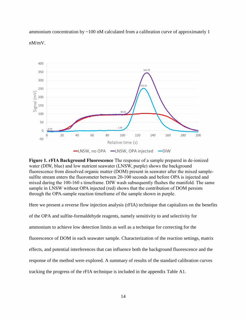
ammonium concentration by ~100 nM calculated from a calibration curve of approximately 1

nM/mV.

Figure 1. rFIA Background Fluorescence The response of a sample prepared in de-ionized

water (DIW, blue) and low nutrient seawater (LNSW, purple) shows the background

fluorescence from dissolved organic matter (DOM) present in seawater after the mixed sample-

sulfite stream enters the fluorometer between 20-100 seconds and before OPA is injected and

mixed during the 100-160 s timeframe. DIW wash subsequently flushes the manifold. The same

sample in LNSW without OPA injected (red) shows that the contribution of DOM persists

through the OPA-sample reaction timeframe of the sample shown in purple.

Here we present a reverse flow injection analysis (rFIA) technique that capitalizes on the benefits

of the OPA and sulfite-formaldehyde reagents, namely sensitivity to and selectivity for

ammonium to achieve low detection limits as well as a technique for correcting for the

fluorescence of DOM in each seawater sample. Characterization of the reaction settings, matrix

effects, and potential interferences that can influence both the background fluorescence and the

response of the method were explored. A summary of results of the standard calibration curves

tracking the progress of the rFIA technique is included in the appendix Table A1.

15

2. Materials and Methods

2.1 Reagents

All reagents were prepared in either de-ionized water (DIW) polished to > 18.2 MΩ-cm

in a Millipore Milli-Q system or in a 0.25 M borate buffer. To prepare the buffer, boric acid

(Fisher ACS grade) was dissolved in the same DIW and adjusted to a pH of 9.50 with 10 N

sodium hydroxide (Fisher ACS grade). Glassware used for reagent and calibration standard

preparations were thoroughly washed with DIW, rinsed with 10% HCl (Fisher trace metal

grade), and rinsed three times with DIW rinses and three rinses of the solution to be used in order

to minimize atmospheric ammonium contamination (Zhang et al. 1997).

2.1.1 rFIA Reagents

Ortho-phthaldialdehyde (Sigma ≥ 97% HPLC) was dissolved at a ratio of a tenth of a

gram of OPA per 1 mL methanol (Sigma-Aldrich CHROMASOLV® gradient grade for HPLC,

≥99.9%) to minimize the contribution of methanol to the OPA blank signal. Aliquots of

dissolved OPA in methanol were mixed into 1 L volumes of the 0.25 M borate buffer to make

five different solutions with rFIA OPA reagent concentrations at 5 mM intervals from 5-25 mM.

A 5 mM formaldehyde (HCHO) solution was prepared by dissolving 750 µL of HCHO stock

(Fisher ACS grade 37% wt.) in 2 L of the 0.25 M borate buffer. To the HCHO solution, 2.52 g

sodium sulfite (Fisher ACS grade) was added and shaken until dissolved to make a 10 mM SO32-

—5 mM HCHO reagent in the 0.25 M borate buffer. The resulting sulfite-formaldehyde reagent

was found to be stable for several months when stored in dark, high density polyethylene

(HDPE) containers at room temperature.

16

2.1.2 Standards

A primary standard solution composed of 2.4995 x 10-2 M ammonium (ACS reagent

grade ammonium chloride) was used to make a secondary standard (2.5072 x 10-4 M

ammonium) for daily preparation of calibration standards at 0, 250, 500, and 1000 nM using

gravimetrically calibrated volumetric flasks and pipets. Calibration standards were made in

unfiltered and aged low-nutrient seawater (LNSW) collected from offshore Gulf of Mexico

surface waters. Calibration standards of the same nutrient concentrations were also made in DIW

and aged LNSW diluted with DIW for the comparison of the slopes of the calibration curves at a

range of salinities (S) between 0 (DIW) and 38 (LNSW) for matrix effect investigation.

The rFIA OPA reagent and calibration standards were contained in 240 mL polyethylene

collapsible sleeves (Playtex) sealed within a polyvinyl chloride (PVC) housing by a silicone O-

ring and PTFE Omnifit™ valve and adapter. Replicate standards and rFIA OPA reagent were

drawn from the sleeves through flanged PTFE fittings with manual valves to minimize

atmospheric contamination.

2.1.3 Interference Solutes

Primary amine and amino acid standards (summarized in Table 1) were made to ~2.5 x

10-4 M in DIW from stocks of ethanolamine (Arcos 99%), mono-methylamine hydrochloride

(Aldrich), L-serine (Sigma SigmaUltra >99% TLC), L-tyrosine (Sigma), L-alanine (Sigma

minimum 98%), L-leucine (Sigma minimum 98%), L-phenylalanine (Sigma minimum 98%), L-

tryptophan (Sigma, sigma grade), B-alanine (Aldrich 99% assay), and glycine (Sigma Ultra

>99% titration). Ammonium high standards prepared in DIW were spiked with each solutions of

amino acids to make a solution that were 1 µM in ammonium and 1 µM in an amino acid for

interference characterization. Additionally, DIW blanks were spiked with each primary amine or

17

amino acid to make 2 µM amino compound solutions that contained no added ammonium. Glass

vials (30 mL screw cap) for these solutions were soaked in 10 % HCl overnight and rinsed with

DIW prior to use.

2.1.4 GD-FIA Reagents

Reagents for the GD-FIA control technique were made with a modification of Jones

(1991), doubling the OPA concentration in the OPA reagent to 1.5 mM. The 1.5 mM GD-FIA

OPA reagent was made using 200 mg OPA (Sigma ≥ 99% HPLC) dissolved in 2 mL methanol

and added into 1 L 0.25 M borate buffer and along with 500 µL 2-mercaptoethanol (Sigma). The

reagent was aged for at least 48 hours to allow for a decay of the background signal and was

stable for an additional 5 days before the reagent to become unusable. The 2% sulfuric acid

(Fisher ACS plus) carrier was made fresh daily, while the 0.7 M NaOH-sodium citrate solution

made from 200 g sodium citrate (Fisher certified) and 18.0 g sodium hydroxide (Fisher ACS)

dissolved in 950 mL of DIW was stable.

2.2 Manifold Description

The fluorometric ammoniuim analyzer consisted of a manifold for the experimental rFIA

technique and an additional manifold for the GD-FIA technique that served as a control. A

schematic of the manifolds modified from the 3-channel nitrogen sensor developed by Masserini

and Fanning (2000) is depicted in Figure 2. The upper panel depicts the rFIA technique for

ammonium analysis. The lower panel shows the GD-FIA technique used as a control. For both

manifolds, a 16 channel peristaltic pump (Ismatec IPC-16) drew the wash, sample/standards and

reagent solutions from their reservoirs at 25% pump speed through PVC pump tubes. Pump

tubes were fitted onto barbed connectors with ¼”-28 threaded zero-dead-volume flange fittings.

The remainder of the analytical manifolds consisted of 0.8 mm inner diameter PTFE tubing. A

18

series of manual 2-way valves (Hamilton HV Plug Valve) at the beginning of the manifolds

allowed for selection between blanks, calibration standards, and samples for analysis drawn from

the collapsible sleaves as an alternative to the use of an autosampler probe drawing from glass

vials.

Figure 2. rFIA and control (GD-FIA) manifold. Manifold schematic for the reverse flow

injection analysis technique (rFIA, upper) and the control gas-diffusion flow injection analysis

technique (GD-FIA, lower). Standards are drawn from the PVC housed PETE collapsible

sleeves, manually selected with two way valves labeled A-D. An autosampler can also be fitted.

The sample stream selection valve alternates between drawing sample and DIW wash. Flow rates

within the pump diagram are in mL/min. The OPA injection loop is ~0.15 mL in volume. The

OPA injection valve loads the injection loop with OPA and adds the contents of the loop to the

carrier stream upon actuation. Dashed lines within the valves indicate the “sample” and “inject”

positions. The mixing coil in the heater is approximately 2 mL in volume. The overall length of

the rFIA system is ~5 m. The control manifold is described in Masserini and Fanning (2000).

2.2.1 rFIA Experimental Manifold

During the “wash” step, DIW was directed through the sample stream selection valve (2-

position 6-port valve, VICI Cheminert) to the manifold while the analyte stream was directed

from the sampler tee fitting, through the valve and pump to waste. The sample stream selection

valve in the “sample” position redirected the analyte stream to the manifold where it mixed with

19

the sulfite-formaldehyde reagent at a second tee fitting, timed to prevent the introduction of an

intersample air bubble. The mixed analyte stream was directed through the OPA injection valve

(2-position 6-port, VICI Cheminert) in the “load” position to the heater. Concurrently, the rFIA

OPA reagent stream was directed through the 0.15 mL injection loop and to waste. In the

“inject” position, the rFIA OPA reagent within the injection loop was incorporated within the

mixed analyte stream and was directed to the heater.

Temperature control was achieved through a PID controller (Watflow Anafaze CLS204)

which limits power to the heater to keep temperature within ± 0.1 °C. To minimize bubble

formation at temperatures above 60 °C, the analyte stream was degassed (Alltech On-line

Degassing System 2000) before passing through 400 cm of PTFE tubing coiled around a heating

block assembly within an insulated enclosure (VICI® Valco Instruments Co. Inc. HVE2). A

PTFE bubble trap (Omnifit) removed gas bubbles from the analyte stream formed in the heating

process. The Hitachi L-7480 fluorometer equpped with adjustable excitation and emission

monochrometers, a photomultiplier tube, and a 40 µL quartz flow cell served as the detector.

Excitation and emission wavelengths were set to 365 and 425 nm, respectively. The

photomultiplier tube was set at its highest sensitivity “1,” and signal averaging was 2 seconds.

2.2.2 GD-FIA Control Manifold

The modified version of a GD-FIA technique (Jones 1991) was run simultaneously for

experiments as a control method for comparative analysis of the rFIA performance. Upstream of

the sample selection valve, a tee was fitted to split the analyte stream to both rFIA and the GD-

FIA control manifolds. The manifold and operational procedure of the GD-FIA control technique

were unchanged from their original configuration with the exception of a doubling of the OPA

concentration (Masserini and Fanning 2000).

20

2.3 Procedure

Concord V2.8 software (A.I. Scientific) was programmed to run the AIM 1250

autosampler MkII relays (A.I Scientific), which then control the valve actuators (VICI®). At 0

seconds, the sample selection valve was set to “wash” and the rFIA OPA injection valve set to

“load” to purge the manifold and rFIA OPA injection loop of any residual analyte. After 60

seconds of DIW wash, the sample selection valve was actuated to the “sample” position during

which a background fluorescence signal of the mixed analyte (sample and sulfite) without OPA

was established. At 185 seconds the rFIA OPA injection valve was actuated to “inject,” allowing

the reaction between the 0.15 mL rFIA OPA reagent and the mixed analyte to occur through the

heating coil. After an additional 15 seconds, both valves were switched back to the respective

“wash/load” position. The total elapsed time for each sample was 200 seconds. 10% HCl was

used to flush the instrument manifold whenever baseline stability degradation was observed.

A Universal Data Collection (UDC) data acquisition package developed in-house on

National Instruments LabView™ software (Masserini 2005) recorded the signal from the

fluorometer, identifying the background fluorescence shoulder height and the uncorrected peak

height of the rFIA OPA-analyte reaction. The peak heights were corrected for background

fluorescence due to DOM in seawater samples and standards by subtracting the shoulder height

from the uncorrected peak height value. Reagent blank corrections were applied to samples and

standards by subtracting the average of the DIW replicates with no background fluorescence.

The average of triplicate un-spiked LNSW blanks corrected for background and reagent (DIW

blanks) fluorescence contributions was subtracted from standards to account for analyte present

in the solvent matrix. Standard calibration curves were constructed and recorded by the UDC

software when running standards. The software calculated the linear least squares regression of

21

the corrected standards and displayed the results in a graphic user interface (Figure 3). The

corrected peak heights of samples were then multiplied by the slope of the curve (units in

nM/mV) to produce actual ammonium concentrations in the samples. The UDC software

allowed for discrete analysis of unknown samples, automatically correcting for background

fluorescence and reagent blank values. Raw data and processed data were stored in separate text

files (.raw, .pkv, .cnc). Similar calculations were performed for the GD-FIA technique with the

exception of the background fluorescence correction.

Figure 3. Universal Data Collection Ammonium Calibration Curve Display. Merged display

of the Universal Data Collection (UDC) software graphic user interface displaying the raw data

(top), linear regression (bottom left) and residuals (bottom right) of a standard calibration with

duplicate standards made in low nutrient seawater using 25 nM OPA at 45 °C. The lower panels

become available in separate windows post-processing. Peaks of the 250, 500, and 1000 nM

ammonium standards are indicated by blue vertical lines in the upper panel, background

fluorescence by red vertical lines. The equation for the calibration curve (in nM/mV) and the r2

value for the linear regression are inset in the lower left panel (y = 2.356 nM/mV x – 0.096 nM;

r2 = 0.9995). The residuals (standard deviation of residuals = 8.9 nM) are inset in the lower right

panel.

22

3. Results for the rFIA Ammonium Method

The results of even the initial rFIA reaction parameters (25 mM OPA, 45° C) displayed

in Figure 3 suggested that these conditions are suitable for sub-micromolar ammonium

measurements. Values for the average peak heights of LNSW were 162.5 ± 12.5 mV with a limit

of detection (LOD) of 7 nM, calculated as three times the standard deviation of the blanks times

the slope 2.356 nM/mV (IUPAC 1997). However, the sensitivity under these conditions was low

and a 34% difference between the DIW and LNSW blank values was observed where DIW

appeared to have greater ammonium present than LNSW, both of which were further examined.

Saturation of the fluorometer occurs at signals beyond 1500 mV, and temperature, reagent

concentration, and flow rates were investigated to produce a 1000 mV signal for the high

standard while minimizing the signal of the blank. A calibration curve slope of 1 nM/mV was

determined to be a reasonable compromise between the upper limit of the instrument response,

resolution across the dynamic range, and sensitivity.

3.1 Reaction Conditions

Reaction temperature and rFIA OPA concentrations strongly influenced analytical

response. Flow rates of the sample and sulfite streams also influenced system performance by

affecting the mixing and dispersion of the sample and reagents and the duration of the analyte

reaction within the heating manifold. These three parameters were systematically checked for

optimal conditions. Discrete analysis of LNSW blanks and standard curves were run at 42.5, 45,

50, 55, 60, 65, and 70 °C and for OPA concentrations of 5, 10, 15, 20, and 25 mM. Results of the

effects of temperature and rFIA OPA concentration are displayed in Figure 4. The response of

DIW reagent blanks was explored at 60 °C for the 5-25 mM range of rFIA OPA concentrations

23

(inset to Figure 4). The 55-65 °C temperature range and 10-15 mM OPA concentration range

meet the desired conditions for optimal method performance for sensitivity and dynamic range.

Figure 4. Slope variation with respect to temperature and OPA concentration. Standard

calibration curve slopes (in nM/mV) were calculated from ammonium standards prepared in low

nutrient seawater (LNSW) and run by the reverse flow injection analysis (rFIA) technique at

temperatures between 42 and 70 °C and 5-25 mM OPA concentrations. The combination of

higher temperature and OPA concentrations saturated the fluorometer, therefore slope

interpolations were used from the blanks and lower concentration standards that were not off

scale. Similarly, low temperatures and low OPA concentrations would not produce meaningful

calibration curves, hence slopes at some concentrations were not directly comparable (i.e. 25

mM OPA and 10 mM OPA). Emphasis was placed on reactions that achieved a reasonable

compromise between resolution and sensitivity identified as a slope of 1 mV/nM. The blue

rectangle encloses conditions that were close to the desired sensitivity and were within the

operating thresholds of the instrument: temperatures between 55 and 65 °C and 5-15 mM OPA.

The inset indicates OPA reagent DIW blank values increased substantially with increasing OPA

concentrations at 60 °C.

0.0

0.5

1.0

1.5

2.0

2.5

3.0

3.5

4.0

4.5

5.0

40 45 50 55 60 65 70 75

Slo

pe

(nM

/mV

)

Temperature (°C)

5 mM 10 mM 15 mM 20 mM 25 mM

0

500

1000

5 15 25

Sig

nal

(m

V)

OPA conentration (mM)

OPA blanks at 60 °C

24

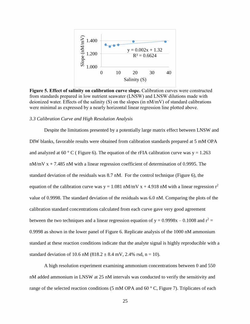
3.2 Reagent Blanks and Matrix Effects

DIW blanks and LNSW blanks were analyzed at the beginning of every calibration to

provide a value for the reagent blank and matrix correction for standards and samples.

Discrepancies in the blank values of up to 34% difference between DIW and LNSW (as

indicated in the summary of Figure 3 in the second row of Table A1) led to an investigation of

the matrix effects on the rFIA technique: standards were made in LNSW and in LNSW diluted

with DIW to cover a full salinity range (S = 2.5-38). The results of these matrix effects tests are

displayed in Figure 5 and were obtained at 60 °C with 5 mM OPA and achieved calibration

curve slopes across the salinity range at approximately 1 nM/mV with low reagent blank

fluorescence values. The slope of the regression in Figure 5 was 0.002 nM/mV S-1 with a

coefficient of determination (r2) at 0.6624. The percent error of the calibration curve slopes of

the dilutions compared to the slope of standards in LNSW were calculated with the equation 1.

Equation 1: 𝑆𝑙𝑜𝑝𝑒𝑑𝑖𝑙𝑢𝑡𝑖𝑜𝑛− 𝑆𝑙𝑜𝑝𝑒𝐿𝑁𝑆𝑊

𝑆𝑙𝑜𝑝𝑒𝐿𝑁𝑆𝑊× 100%.

Percent error did not exceed the 5.9% of undiluted LNSW standard calibrations conducted two

days apart (Table A1: rows 3-10, column 6). Salinity had minimal effect on the calibration

curves at the 5 mM OPA concentration. The discrepancy in the DIW reagent blank and the

solvent matrix blanks also decreased from approximately 20% to 1.2% as the salinity of the

solvent matrix blank also decreased (Table A1: rows 3-10 column 15).

25

Figure 5. Effect of salinity on calibration curve slope. Calibration curves were constructed

from standards prepared in low nutrient seawater (LNSW) and LNSW dilutions made with

deionized water. Effects of the salinity (S) on the slopes (in nM/mV) of standard calibrations

were minimal as expressed by a nearly horizontal linear regression line plotted above.

3.3 Calibration Curve and High Resolution Analysis

Despite the limitations presented by a potentially large matrix effect between LNSW and

DIW blanks, favorable results were obtained from calibration standards prepared at 5 mM OPA

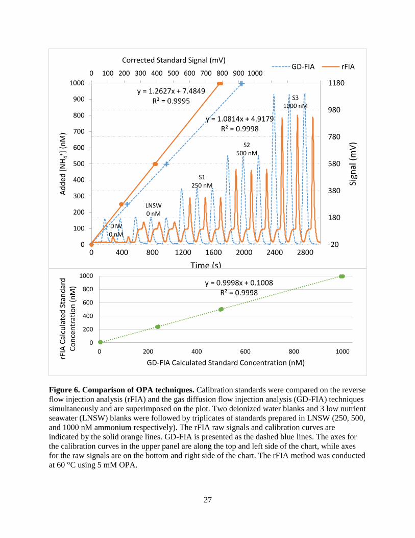
and analyzed at 60 ° C ( Figure 6). The equation of the rFIA calibration curve was y = 1.263

nM/mV x + 7.485 nM with a linear regression coefficient of determination of 0.9995. The

standard deviation of the residuals was 8.7 nM. For the control technique (Figure 6), the

equation of the calibration curve was y = 1.081 nM/mV x + 4.918 nM with a linear regression r2

value of 0.9998. The standard deviation of the residuals was 6.0 nM. Comparing the plots of the

calibration standard concentrations calculated from each curve gave very good agreement

between the two techniques and a linear regression equation of y = 0.9998x – 0.1008 and r2 =

0.9998 as shown in the lower panel of Figure 6. Replicate analysis of the 1000 nM ammonium

standard at these reaction conditions indicate that the analyte signal is highly reproducible with a

standard deviation of 10.6 nM (818.2 ± 8.4 mV, 2.4% rsd, n = 10).

A high resolution experiment examining ammonium concentrations between 0 and 550

nM added ammonium in LNSW at 25 nM intervals was conducted to verify the sensitivity and

range of the selected reaction conditions (5 mM OPA and 60 ° C, Figure 7). Triplicates of each

y = 0.002x + 1.32

R² = 0.6624

1.000

1.200

1.400

0 10 20 30 40

Slo

pe

(nM

/mV

)Salinity (S)

26

addition had a very low inter-sample standard deviation (the standard deviations of each set of

triplicate samples were averaged and multiplied by the slope for 2.7 nM rsd = 1.4%) and were

clearly distinguishable between intervals. A single tailed s-pooled Student’s t-test was conducted

on the means of the reagent blank (DIW 42.4 ± 0.8 mV) and the matrix blank (LNSW 41.6 ± 0.3

mV); the t-experimental value (0.395) was less than the t-critical value (2.78), indicating that the

DIW and LNSW blanks were similar at a 95% confidence level. The triplicate LNSW blanks had

a standard deviation of 0.3 nM; three times the standard deviation for the replicate blanks gave a

LOD of 1.1 nM.

3.4 Amine and Amino Acid Interference

The interferences from primary amines and amino acids were checked with duplicates of

1000 nM ammonium standards spiked with 1 µM of the target amino compound (listed in section

2.1.4 and Table 2) prepared in DIW. The equivalent ammonium concentration of the spiked

ammonium standards was determined relative to replicates (n = 11) of 1000 nM ammonium

standards prepared in DIW that had not been spiked with the given amino compound. The results

displayed in column 3 of Table 2 ranged from 778 to 1044 nM. Additionally, DIW spiked with 2

µM of the target amino acid were also compared against replicate non-spiked DIW blanks (n =

11) in column 2, with no amino acid resulting in greater than 55 nM ammonium equivalents. The

reaction temperature was reduced to 45 °C, and 10 mM rFIA OPA was used for the rFIA

technique to allow sufficient dynamic range to accommodate for potential saturation of the

fluorometer for combined interferences. Ranges (not listed in Table 2) for the control technique

were very similar with the notable exception of mono-methylamine, which saturated the

fluorometer for both the blank and the spiked standard in the GD-FIA measurement, but not for

the rFIA technique.

27

Figure 6. Comparison of OPA techniques. Calibration standards were compared on the reverse

flow injection analysis (rFIA) and the gas diffusion flow injection analysis (GD-FIA) techniques

simultaneously and are superimposed on the plot. Two deionized water blanks and 3 low nutrient

seawater (LNSW) blanks were followed by triplicates of standards prepared in LNSW (250, 500,

and 1000 nM ammonium respectively). The rFIA raw signals and calibration curves are

indicated by the solid orange lines. GD-FIA is presented as the dashed blue lines. The axes for

the calibration curves in the upper panel are along the top and left side of the chart, while axes

for the raw signals are on the bottom and right side of the chart. The rFIA method was conducted

at 60 °C using 5 mM OPA.

y = 1.0814x + 4.9179R² = 0.9998

y = 1.2627x + 7.4849R² = 0.9995

0 100 200 300 400 500 600 700 800 900 1000 1100 1200 1300 1400

0

100

200

300

400

500

600

700

800

900

1000

-20

180

380

580

780

980

1180

0 400 800 1200 1600 2000 2400 2800

Corrected Standard Signal (mV)A

dd

ed [

NH

4+ ]

(n

M)

Sign

al (

mV

)

Time (s)

GD-FIA rFIA

DIW 0 nM

LNSW 0 nM

S1 250 nM

S2 500 nM

S3 1000 nM

y = 0.9998x + 0.1008R² = 0.9998

0

200

400

600

800

1000

0 200 400 600 800 1000

rFIA

Cal

cula

ted

Sta

nd

ard

C

on

cen

trat

ion

(n

M)

GD-FIA Calculated Standard Concentration (nM)

28

Figure 7. High resolution analysis. Triplicate of samples prepared in LNSW at 25 nM intervals

from 0-500 nM ammonium concentrations were analyzed at 5 mM OPA and 60 °C to examine

the resolution and sensitivity of the rFIA technique. The eleventh sample signal suffered from

noise as the result of a bubble passing through the flow cell, and was removed from analysis.

Table 2. Potential interference from primary amines and amino acids. The equivalent

ammonium concentration of the average values of listed potentially interfering species at 2 µM

(n = 2) prepared in DIW are displayed in column 2. The third column displays the equivalent

ammonium concentration of average signals of 1000 nM ammonium standards, spiked with 1

µM AC concentration, prepared in DIW. Replicates (n = 11) of DIW blanks and 1000 nM

ammonium standards served as the calibration curve endpoints (rFIA slope = 2.359 nM/mV. The

experiments were conducted at 45 °C with 10 mM OPA. Primary Amine,

Amino Acid

Ammonium equivalents (nM) of 2 µM interfering

species in DIW

Ammonium equivalents (nM) of 1 µM

interfering species spiked in 1 µM NH4+

standard

Ethanolamine 54.1 ± 36.2 945.1 ± 34.4

Methylamine 9.0 ± 14.5 815.7 ± 120.4

L-serine 23.5 ± 15.3 778.1 ± 173.6

L-tyrosine 12.2 ± 2.7 840.2 ± 51.0

L-alanine 14.6 ± 35.0 1044.9

L-leucine 19.3 ± 22.0 868.8 ± 17.8

L-phenylalanine 10.5 ± 3.5 881.9

L-tryptophan 19.1 ± 3.7 893.5 ± 66.4

B-alanine 0.4 ± 1.0 961.4 ± 23.3

Glycine 30.4 ± 60.4 912.0 ± 91.5

4. Discussion

Flow injection analysis and variations of FIA rely on carefully controlled timing. It is

essential that the reaction starts and proceeds to the same extent, for the same period of time,

225

250

275

300

325

350

375

400

425

450

475

500

29

with the same delivery of reagents in order for every sample to be comparable (Ruzicka and

Hansen, 1978). So long as these requirements are met, and there are few flow issues, no leakages

(as commonly happens with the GD-FIA PTFE membranes (Van Der Linden, 1983), and reagent

stability outlasts the duration of the analysis, it is not necessary to know the precise reaction

conditions. Nonetheless, great effort has gone into understanding the reaction conditions for

optimization of the rFIA technique for ammonium analysis. rFIA allows for the reproducibility

of the reaction conditions common to FIA with the added benefit of producing a background

signal for every sample, enabling corrections for the background fluorescence of seawater

samples.

4.1 Temperature and OPA Concentration

The initial 34% difference between DIW reagent blanks and LNSW solvent blanks

observed at OPA concentrations of 25 mM and a temperature at 45 °C led to experimentation to

discover the cause of the difference. DIW reagent blanks produced too high of a signal, and

subtraction of the reagent blank would result in negative values for the LNSW solvent blank and

any low ammonium samples. Decreasing the OPA concentration lowers the reagent blank values,

but also decreases sensitivity as the available OPA reacts less during the ~80 seconds of mixing

and diffusion allowed to occur after the OPA is injected. Increased temperature at lowered OPA

concentrations offered an appropriate compromise between lower blank values and adequate

sensitivity. At OPA concentrations of 5-15 mM and temperatures between 55 and 65 °C, slopes

were close to the ideal selected slope of 1 nM/mV. Temperatures above 60 °C forced dissolved

gases out of solution and required the use of an on-line degasser and bubble trap to reduce noise

in the baseline and occasional spikes in the signals due to air bubbles passing through the

fluorometer. At the 60 °C and 5 mM OPA parameters, linear results were obtained and a low

30

limit of detection of 1.1 nM were produced, a six fold improvement compared to the previous 45

°C, 25 mM OPA result (LOD = 7 nM). The differences in the blank values for both DIW and

LNSW showed much less disparity and were insignificant at the 95% confidence level. .

Validation of the new setting was conducted by running the GD-FIA control method

concurrently and the techniques had very good agreement (r2 = 0.9998 as shown in the lower

panel of Figure 6).

4.2 Background Fluorescence

The importance of correcting for background fluorescence is well established.

Background fluorescence of dissolved organic material was corrected for manually in Holmes et

al. (1999) by subtracting the measured signal of the analyte mixed the sulfite reagent without

OPA from the sulfite reagent with OPA. Similar corrections were conducted by Aminot et al.

(2001) on the FIA system by allowing the analyte to continue without reacting with OPA. Bey et

al. (2011) devised a multichannel instrument that could make the same measurements with and

without OPA through a FIA technique using sulfite and perform a background fluorescence

correction for all samples automatically. However, like the manual and FIA techniques, it

requires the preparation of an additional reagent, potentially introducing errors from differences

in the reagents with and without OPA. Reverse flow injection analysis simplifies the correction

procedure in a two-step process: 1. it establishes a background fluorescence signal by streaming

the sample with the sulfite-HCHO reagent through the fluorometer without OPA, and 2. it

subtracts the background fluorescence signal from the height of the signal of the analyte stream

that had reacted with injected OPA.

31

4.3 Blanks and Matrix Effects

Further investigation into the initial 34% difference in fluorescence between DIW and

LNSW indicated minimal salinity effects (< 6%) on the slopes of standard curves prepared in the

various LNSW dilutions. Discrepancies in matrix effects have been previously reported, ranging

from minimal effects (Amornthammarong and Zhang 2008), to an elevated response of DIW

relative to seawater (Kerouel and Aminot 1997, Holmes et al. 1999, Watson et al. 2005), to a

suppressed DIW response relative to LNSW (Jones 1991, Aminot et al. 2001, Bey et al. 2011).

Although there were some inconsistencies in magnitude and direction of reported matrix effects,

this general trend applies: matrix effects have greater impact on measurements of samples with

lower concentrations of ammonium. The minimal effects reported here agree with the

Amornthammarong and Zhang (2008) technique from which the OPA-sulfite-formaldehyde

chemistry was adapted for rFIA. This technique is tailored for use in the oligotrophic ocean

where salinity is relatively consistent across a given gyre or basin. Therefore, the use of LNSW

as the solvent for standard preparation is recommended to minimize matrix effects for rFIA

ammonium measurements in seawater. This recommendation runs contrary to the use of DIW by

Amornthammarong and Zhang (2008), but agrees with Zhang et al. (1997) for colorimetric

determination of ammonium below 1.2 µM. The selection of the LNSW solvent matrix as the

reagent blank has a precedent in the Environmental Protection Agency Method 349.0 for

colorimetric analysis of ammonium below 1.2 µM (Zhang et al. 1997).

4.4 Limit of Detection

Limits of detection in this work are three times the standard deviation of replicate blanks

times the slope of the calibration curve, similar to the approach of Aminot et al. (1997) and

Amornthammarong and Zhang (2008). This method had a LOD as low as 1.1 nM ammonium

32

from the 25 nM interval high resolution experiment. The background fluorescence correction

permitted by rFIA makes these very low limits of detection possible. Without it, the calculated

ammonium in the low nutrient seawater would be artificially high (118.1 nM) due to the

background fluorescence, and these low limits of detection would be unattainable. Standard

deviations of replicate blanks (DIW for other works, LNSW for this one) to determine detection

limit do not reflect how temperature effects on mid- and high-range analyte values and their

impacts on the calibration slope. The relative standard deviation of higher ammonium standards

indicates consistency of performance at those concentrations. The average of the standard

deviations for all the triplicates of the high resolution experiment was 3.2 nM, 1.4% of the

signals, while the standard deviation for replicates of the 1000 nM ammonium standard was 10.6

nM, 2.4% relative standard deviation, indicating high reproducibility across the analytical range.

4.5 Potential Interferences

Amino acids and primary amines found in seawater may potentially react with OPA and

modify the ammonium signal if the reaction product fluoresces at similar excitation/emission

wavelengths (325/465 nm, respectively). The sulfite-formaldehyde reagent was adopted for the

rFIA technique because it was reported to increase the selectivity of OPA for ammonium over

potential interferences by amines and amino acids (Amornthammarong and Zhang 2008). Solutes

of 2 µM of the potentially interfering species only produced a signal ≤ 34% of the DIW blank,

and only 3.5% of the 1000 nM ammonium standard. The equivalent ammonium concentration of

spiked standards presented in Table 2 ranged from 778 to 1044 nM compared to the 1000 nM

ammonium standard. The general suppression of the ammonium signal by these amines has also

been reported by Bey et al. (2011), who attributed the suppression to the formation of an adduct

between the sulfite, OPA, ammonium, and the amine which may exhibit maximum fluorescence

33

at wavelengths shifted away from those selected for this method. The GD-FIA control method

produced similar range and magnitude of results as the rFIA method with the exception of mono-

methylamine, which saturated the fluorometer for all tests on the gas diffusion technique. The

small molecule mono-methylamine has also been known to permeate PTFE membranes in the

gas diffusion techniques (Jones 1991) and was also problematic in the results of Bey et al. (2011)

producing an approximate 53% yield. Furthermore, they reported a 4 percent yield for

ethanolamine (suppression of signal by 96%). A 72% response relative to an ammonium

standard shown in Amornthammarong and Zhang (2008) differs in how the measurement was

obtained (i.e. a comparison of the reaction of 1 µM ethanolamine independent of a 1 µM

ammonium versus the direct analysis of the spiked standard analyzed here). The 2 µM

ethanolamine blank analyzed via rFIA only had a 5.8 % relative response, a 12 fold reduction in

potential interference. The sulfite-HCHO chemistry for rFIA OPA injection discriminates against

the interaction of amines and amino acids with OPA, allowing for a nearly full signal across the

selection of analyzed compounds. The most common amino acids comprising of dissolved free

amino acid pool (glycine, serine, and alanine) in seawater are not usually present in excess of 50

nM in the Sargasso Sea (Suttle et al. 1991) and at these lower concentrations the effects of

interference on ammonium analysis will be dramatically diminished relative to the 20 and 40

fold concentrations examined here.

5. Conclusions

The reverse flow injection analysis technique presented here combines the stability and

selectivity of a sulfite reagent amended by formaldehyde with the sensitivity of fluorometric

ammonium detection with OPA. This method has demonstrated a detection limit of 1.1 nM

34

ammonium in seawater with simultaneous background fluorescence correction, suitable for the

analysis of the oligotrophic surface ocean for sub-micromolar ammonium concentrations. This

technique represents an improvement in sensitivity over the widely used indophenol blue

colorimetric technique and simplifies corrections for background fluorescence relative to other

fluorometric OPA FIA techniques. Although gas diffusion techniques also avoid background

fluorescence, they suffer from a propensity to develop clogs and leaks within the gas diffusion

block. rFIA needs no membrane separation step. Matrix effects were ameliorated by the use of

aged LNSW for standard preparation. The method is tailored for measurements of sub-

micromolar ammonium concentration in surface waters of the open ocean where salinity

deviations are minimal and the concentrations of amino acids and primary amines are below 50

nM and not likely to interfere with the measurement of ammonium.

Future direction for the rFIA technique for ammonium analysis include a GD-FIA and

rFIA comparison in a field deployment and the potential integration into the 3-channel nitrogen

sensor to replace the GD-FIA technique (Masserini and Fanning 2000) from which the manifold

was derived, making it an all rFIA nanomolar inorganic nitrogen analyzer. Such an analyzer

could provide valuable information about the extent, concentration, and rates of uptake and

release of dissolved inorganic nitrogen compounds in the oligotrophic surface ocean.

6. Acknowledgements

This work was funded in part by the Office of Naval Research Contract N000149615024

and through institutional support from the University of South Florida.

35

Chapter 3: Conclusion

The work presented in Chapter 2 is the culmination of the application of rFIA to the

measurement of nanomolar ammonium concentrations in oligotrophic seawater. The reaction

conditions settled upon in this technique were mixing the sample at a 1:1 flow rate with 10 mM

sulfite-5 mM formaldehyde reagent, injecting the analyte stream with a 5 mM OPA reagent, and

heating the mixed reagent-analyte stream to 60 °C. The results of standard calibration curves at

these conditions indicate a 1.1 nM limit of detection, a slope (sensitivity) of 1.2 nM/mV with a

least square regression fit coefficient of determination better than 0.999 up to 1000 nM

ammonium, and excellent reproducibility (2.4% relative standard deviation for 10 replicate 1000

nM ammonium standards). The rFIA technique enables automatic background fluorescence

corrections to be applied to each sample by streaming analyte through the fluorometer without

OPA to establish the background fluorescence first and subsequently injecting OPA to develop

the analyte signal. The potential contribution of background fluorescence can be as high as 118

nM ammonium equivalents, which if uncorrected would show a systematically and

disproportionately high ammonium concentration at the low concentrations expected in

oligotrophic seawater. The effects of salinity on the solvent matrix was found to be minimal (less

than 6% error between standards prepared in dilutions of LNSW with DIW and standards

prepared in LNSW) Additionally, the selection of the sulfite-formaldehyde chemistry minimizes

the potential interference of 10 tested primary amines and amino acids.

36

The rFIA technique performs as accurately as the well vetted Jones (1991) gas-diffusion

flow injection analysis method (a comparison of slopes of standard calibrations in LNSW

between the two methods resulted in a linear least square regression fit coefficient of

determination of 0.9998). It offers advantages over the GD-FIA method in terms of reagent

stability, ease of use, and elimination of the need for isolating the ammonium using a leak-prone

PTFE membrane separation diffusion block. Fluorescent OPA-based chemistries in general

perform better at nanomolar ammonium concentrations than the widely used colorimetric

indophenol blue (Šraj et al. 2014). As a part of the growing prevalence of FIA for fluorescent

ammonium analysis, automatic batch analyzers, multi-pump sequential injectors, and solid phase

extraction techniques have been paired with the fluorescent detection of ammonium with OPA.

These procedures offer advantages such as power requirements, reagent/sample consumption,

and cost. The 1.1 nM limit of detection offered by rFIA and its relatively high sample throughput

(18 samples per hour) put it on par with these techniques. No other technique, however, offers

the background fluorescence correction in quite the same simple and effective manner as rFIA

does.

The technique still needs to be vetted in a natural setting. A multi-day cruise in the Gulf

of Mexico would be sufficient to prove the validity of the method at sea. The comparison of

samples analyzed on-line and continuously via rFIA and GD-FIA aboard the ship against

discrete samples returned for laboratory analysis with the same techniques and IPB is a short-

term goal. Long-term goals may include the integration of the rFIA technique for ammonium

with the rFIA techniques for nitrate and nitrite for a high resolution multi-channel nitrogen

analyzer from which the ammonium technique was derived (Masserini and Fanning 2000).

37

The future of OPA-based fluorescent techniques is in accurately characterizing the low

concentrations of ammonium in the oligotrophic ocean, where boluses of relatively enriched

ammonium may have a spatial and temporal distributions with ecological significance (Fanning

et al. 2015) that are not measurable by less sensitive techniques such as the IPB method. This can

be achieved through adapting the new technologies to smaller platforms that can operate

independently of an analyst. Moorings and autonomous underwater vehicles are attractive and

relatively less expensive platforms compared to ship-board sample collection. The in-situ

collection of data avoids several potential sources of ammonium contamination and changes to

the sample concentration due to metabolic processes. Mobile and near real-time trace ammonium

data can also provide researchers with information useful for tracking small scale water masses

otherwise indistinguishable by salinity or temperature changes (Masserini 2005, Fanning et al.

2015).

38

References

Aiken, J., J. Cumming, S. Gibb, N. Rees, R. Woodd-Walker, M. Woodward and J. Woolfenden

(1997). "AMT-5 Cruise Report RRS James Clark Ross JR19970914."

Aiken, J. and M. Woodward (1998). "AMT-6 Cruise Report RRS James Clark Ross JR19980514

".

Aminot, A., R. Kérouel and D. Birot (2001). "A flow injection-fluorometric method for the

determination of ammonium in fresh and saline waters with a view to in situ analyses."

Water Research 35(7): 1777-1785.

Aminot, A., D. S. Kirkwood and R. Kerouel (1997). "Determination of ammonia in seawater by

the indophenol-blue method: Evaluation of the ICES NUTS I/C 5 questionnaire." Marine

Chemistry 56(1): 59-75.

Amornthammarong, N., J.-Z. Zhang and P. B. Ortner (2011). "An autonomous batch analyzer for

the determination of trace ammonium in natural waters using fluorometric detection."

Analytical Methods 3(7): 1501-1506.

Amornthammarong, N., J.-Z. Zhang, P. B. Ortner, J. Stamates, M. Shoemaker and M. W. Kindel

(2013). "A portable analyser for the measurement of ammonium in marine waters."

Environmental Science: Processes & Impacts 15(3): 579-584.

Amornthammarong, N. and J. Z. Zhang (2008). "Shipboard fluorometric flow analyzer for high-

resolution underway measurement of ammonium in Seawater." Analytical Chemistry

80(4): 1019-1026.

Aoki, T., S. Uemura and M. Munemori (1983). "Continuous flow fluorometric determination of

ammonia in water." Analytical Chemistry 55(9): 1620-1622.

Bey, S., D. P. Connelly, F. E. Legiret, A. J. K. Harris and M. C. Mowlem (2011). "A high-

resolution analyser for the measurement of ammonium in oligotrophic seawater." Ocean

Dynamics 61(10): 1555-1565.

Bucur, B., M. C. Icardo and J. M. Calatayud (2006). "Spectrophotometric determination of

ammonium by an rFIA assembly." Revue Roumaine De Chimie 51(2): 101-108.

Bushaw, K. L., R. G. Zepp, M. A. Tarr, D. Schulz-Jander, R. A. Bourbonniere, R. E. Hodson, W.

L. Miller, D. A. Bronk and M. A. Moran (1996). "Photochemical release of biologically

available nitrogen from aquatic dissolved organic matter." Nature 381(6581): 404-407.

39

Dortch, Q. (1990). "The interaction between ammonium and nitrate uptake in phytoplankton."

Marine Ecology-Progress Series 61(1-2): 183-201.

Fanning, K., R. T. Masserini, J. J. Walsh, R. Wanninkhof, K. Sullivan, J. I. Virmani and C. A.

Heil (2015). "An ammonium enrichment event in the surface ocean: Wind forcing and

potential ramifications " Marine Chemistry 174: 26-34.

Frank, C. and F. Schroeder (2007). "Using Sequential Injection Analysis to Improve System and

Data Reliability of Online Methods: Determination of Ammonium and Phosphate in

Coastal Waters." Journal of Automated Methods and Management in Chemistry 2007.

Genfa, Z. F. and P. K. Dasgupta (1989). "Flurometric measurement of aqueous ammonium ion in

a flow-injection system." Analytical Chemistry 61(5): 408-412.

Grasshoff, K. and H. Johannsen (1972). "A New Sensitive and Direct Method for the Automatic

Determination of Ammonia in Sea Water." Journal du Conseil 34(3): 516-521.

Harrison, W. G., L. R. Harris and B. D. Irwin (1996). "The kinetics of nitrogen utilization in the

oceanic mixed layer: Nitrate and ammonium interactions at nanomolar concentrations."

Limnology and Oceanography 41(1): 16-32.

Holligan, P., M. Woodward and K. Chamberlain (2005). "AMT-17 Cruise Report RRS

Discovery JR20051015."

Holmes, R. M., A. Aminot, R. Kerouel, B. A. Hooker and B. J. Peterson (1999). "A simple and

precise method for measuring ammonium in marine and freshwater ecosystems."

Canadian Journal of Fisheries and Aquatic Sciences 56(10): 1801-1808.

IUPAC (1997). Compendium of Chemical Terminology. the "Gold Book". A. D. McNaught and

A. Wilkinson. Oxford, Blackwell Scientific Publications.

Jickells, T., M. Woodward and K. Chaimberlain (2003). AMT-12 Cruise Report RRS James

Clark Ross JR20030512

Johnson, M., R. Sanders, V. Avgoustidi, M. Lucas, L. Brown, D. Hansell, M. Moore, S. Gibb, P.

Liss and T. Jickells (2007). "Ammonium accumulation during a silicate-limited diatom

bloom indicates the potential for ammonia emission events." Marine Chemistry 106: 13.

Johnson, M. T., P. S. Liss, T. G. Bell, T. J. Lesworth, A. R. Baker, A. J. Hind, T. D. Jickells, K.

F. Biswas, E. M. S. Woodward and S. W. Gibb (2008). "Field observations of the ocean-

atmosphere exchange of ammonia: Fundamental importance of temperature as revealed

by a comparison of high and low latitudes." Global Biogeochemical Cycles 22(1):

GB1019.

Jones, R. D. (1991). "An improved fluorescence method for the determination of nanomolar

concentrations of ammonium in natural-waters." Limnology and Oceanography 36(4):

814-819.

40

Kerouel, R. and A. Aminot (1997). "Fluorometric determination of ammonia in sea and estuarine

waters by direct segmented flow analysis." Marine Chemistry 57(3-4): 265-275.

Ma, J., L. Adornato, R. H. Byrne and D. Yuan (2014). "Determination of nanomolar levels of

nutrients in seawater." TrAC Trends in Analytical Chemistry 60(0): 1-15.

Ma, J., D. Yuan, M. Zhang and Y. Liang (2009). "Reverse flow injection analysis of nanomolar

soluble reactive phosphorus in seawater with a long path length liquid waveguide

capillary cell and spectrophotometric detection." Talanta 78(1): 315-320.

Mantoura, R. F. C. and E. M. S. Woodward (1983). "Optimization of the indophenol blue

method for the automated determination of ammonia in estuarine waters." Estuarine,

Coastal and Shelf Science 17(2): 219-224.

Masserini, R. T. (2005). Ammonium, nitrate, and nitrite in the oligotrophic ocean: Detection

methods and usefulness as tracers. Ph.D. Dissertation, University of South Florida.

Masserini, R. T. and K. A. Fanning (2000). "A sensor package for the simultaneous

determination of nanomolar concentrations of nitrite, nitrate, and ammonia in seawater by

fluorescence detection." Marine Chemistry 68(4): 323-333.

Menzel, D. W. and J. P. Spaeth (1962). "Occurance of Ammonia in Sargasso Sea Waters and in

Rain Water at Bermuda." Limnology and Oceanography 7(2): 159-162.

Molins-Legua, C., S. Meseguer-Lloret, Y. Moliner-Martinez and P. Campíns-Falcó (2006). "A

guide for selecting the most appropriate method for ammonium determination in water

analysis." TrAC Trends in Analytical Chemistry 25(3): 282-290.

Olson, T. M. and M. R. Hoffmann (1989). "Hydroxyalkylsulfonate formation: Its role as a S(IV)

reservoir in atmospheric water droplets." Atmospheric Environment (1967) 23(5): 985-

997.

Pilson, M. E. Q. (1998). An Introduction to the Chemistry of the Sea. Upper Saddle River, NJ,

Prentice-Hall, Inc.

Redfield, A., B. H. Ketchum and F. A. Richards (1963). The Sea, Interscience.

Robinson, C. and E. M. S. Woodward (2003). "AMT-13 Cruise Report RRS James Clark Ross

JR20030910 ".

Roth, M. (1971). "Fluorescence reaction for amino acids." Analytical Chemistry 43(7): 880-882.

Růžička, J. and E. H. Hansen (1978). "Flow injection analysis : Part X. theory, techniques and

trends." Analytica Chimica Acta 99(1): 37-76.

Schlesinger, W. H. (2007). San Diego, Academic Press.

41

Schlesinger, W. H. (2007). Chapter 12 - The Global Cycles of Nitrogen and Phosphorus.

Biogeochemistry (Second Edition). W. H. Bernhardt. San Diego, Academic Press: 383-

401.

Schlitzer, R., P. Monfray and N. Hoepffner (2003). Joint Global Ocean Flux Study Report No.

38. Global Ocean Productivity and the Fluxes of Carbon and Nutrients: Combining

Observations and Models. Ispra, Italy, EC Joint Research Centre.

Solorzano, L. (1969). "Determination of ammonia in natural waters by phenolhypochlorite

method." Limnology and Oceanography 14(5): 799-&.

Šraj, L. O. C., M. I. G. S. Almeida, S. E. Swearer, S. D. Kolev and I. D. McKelvie (2014).

"Analytical challenges and advantages of using flow-based methodologies for ammonia

determination in estuarine and marine waters." TrAC Trends in Analytical Chemistry

59(0): 83-92.

Suttle, C. A., A. M. Chan and J. A. Fuhrman (1991). "Dissolved free amino acids in the Sargasso

Sea: uptake and respiration rates, turnover times, and concentrations." Marine Ecology-

Progress Series 70: 11.

US EPA. (2013). Aquatic Life Ambient Water Quality Criteria for Ammonia - Freshwater.

Washington D.C., EPA.

Van Der Linden, W. E. (1983). "Membrane separation in flow injection analysis : Gas

Diffusion." Analytica Chimica Acta 151(0): 359-369.

Watson, R. J., E. C. V. Butler, L. A. Clementson and K. M. Berry (2005). "Flow-injection

analysis with fluorescence detection for the determination of trace levels of ammonium in

seawater." Journal of Environmental Monitoring 7(1): 37-42.

Woodward, E. M. S. and V. Kitidis (2000). "AMT-11 Cruise Report RRS James Clark Ross

JR20000912 ".

Woodward, M. and C. Harris (2008). "AMT-18 Cruise Report RRS James Clark Ross

JR20081003 ".

Zhang, J. Z., P. B. Ortner, C. J. Fischer and L. D. Moore Jr. (1997). "Method 349.0."

Determination of ammonia in estuarine and coastal waters by gas segmented continuous

flow colorimetric analysis.

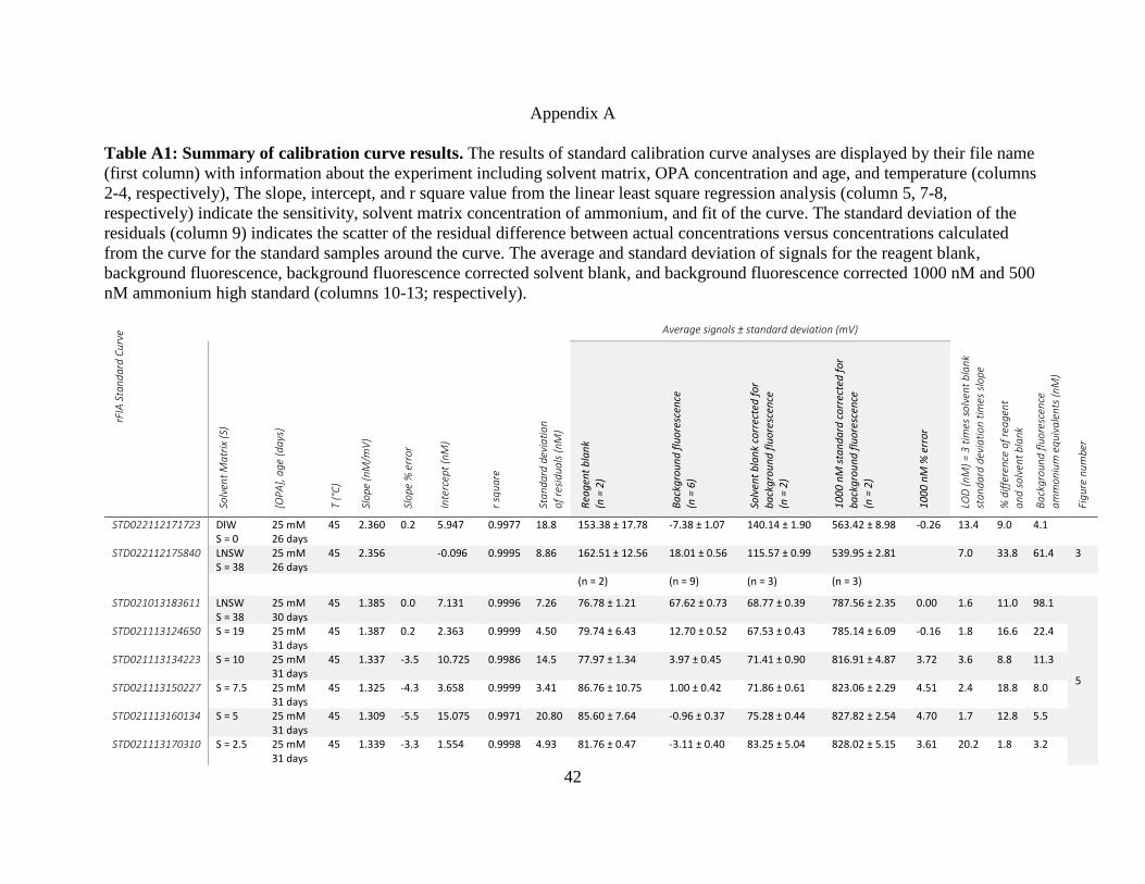
42

Appendix A

Table A1: Summary of calibration curve results. The results of standard calibration curve analyses are displayed by their file name

(first column) with information about the experiment including solvent matrix, OPA concentration and age, and temperature (columns

2-4, respectively), The slope, intercept, and r square value from the linear least square regression analysis (column 5, 7-8,

respectively) indicate the sensitivity, solvent matrix concentration of ammonium, and fit of the curve. The standard deviation of the

residuals (column 9) indicates the scatter of the residual difference between actual concentrations versus concentrations calculated

from the curve for the standard samples around the curve. The average and standard deviation of signals for the reagent blank,

background fluorescence, background fluorescence corrected solvent blank, and background fluorescence corrected 1000 nM and 500

nM ammonium high standard (columns 10-13; respectively).

rFIA

Sta

nd

ard

Cu

rve

Solv

ent

Ma

trix

(S)

[OP

A],

age

(d

ays

)

T (°

C)

Slo

pe (

nM/m

V)

Slo

pe %

err

or

Inte

rcep

t (n

M)

r sq

uar

e

Sta

nd

ard

dev

iati

on

of

resi

dua

ls (

nM)

Average signals ± standard deviation (mV)

LOD

(n

M)

= 3

tim

es s

olv

ent

bla

nk

sta

nd

ard

dev

iati

on

tim

es s

lope

% d

iffe

renc

e of

rea

gen

t

an

d s

olv

ent

bla

nk

Ba

ckgr

oun

d f

luo

resc

ence

am

mo

niu

m e

qui

vale

nts

(n

M)

Fig

ure

num

ber

Rea

gen

t b

lan

k

(n =

2)

Ba

ckg

rou

nd

flu

ore

scen

ce

(n =

6)

Solv

ent

bla

nk

corr

ecte

d f

or

ba

ckg

rou

nd

flu

ore

scen

ce

(n =

2)

10

00

nM

sta

nd

ard

co

rrec

ted

fo

r b

ack

gro

un

d f

luo

resc

ence

(n =

2)

10

00

nM

% e

rro

r

STD022112171723 DIW S = 0

25 mM 26 days

45 2.360 0.2 5.947 0.9977 18.8 153.38 ± 17.78 -7.38 ± 1.07 140.14 ± 1.90 563.42 ± 8.98 -0.26 13.4 9.0 4.1

STD022112175840 LNSW S = 38

25 mM 26 days

45 2.356 -0.096 0.9995 8.86 162.51 ± 12.56 18.01 ± 0.56 115.57 ± 0.99 539.95 ± 2.81 7.0 33.8 61.4 3

(n = 2) (n = 9) (n = 3) (n = 3)

STD021013183611 LNSW S = 38

25 mM 30 days

45 1.385 0.0 7.131 0.9996 7.26 76.78 ± 1.21 67.62 ± 0.73 68.77 ± 0.39 787.56 ± 2.35 0.00 1.6 11.0 98.1

5

STD021113124650 S = 19 25 mM 31 days

45 1.387 0.2 2.363 0.9999 4.50 79.74 ± 6.43 12.70 ± 0.52 67.53 ± 0.43 785.14 ± 6.09 -0.16 1.8 16.6 22.4

STD021113134223 S = 10 25 mM 31 days

45 1.337 -3.5 10.725 0.9986 14.5 77.97 ± 1.34 3.97 ± 0.45 71.41 ± 0.90 816.91 ± 4.87 3.72 3.6 8.8 11.3

STD021113150227 S = 7.5 25 mM 31 days

45 1.325 -4.3 3.658 0.9999 3.41 86.76 ± 10.75 1.00 ± 0.42 71.86 ± 0.61 823.06 ± 2.29 4.51 2.4 18.8 8.0

STD021113160134 S = 5 25 mM 31 days

45 1.309 -5.5 15.075 0.9971 20.80 85.60 ± 7.64 -0.96 ± 0.37 75.28 ± 0.44 827.82 ± 2.54 4.70 1.7 12.8 5.5

STD021113170310 S = 2.5 25 mM 31 days

45 1.339 -3.3 1.554 0.9998 4.93 81.76 ± 0.47 -3.11 ± 0.40 83.25 ± 5.04 828.02 ± 5.15 3.61 20.2 1.8 3.2

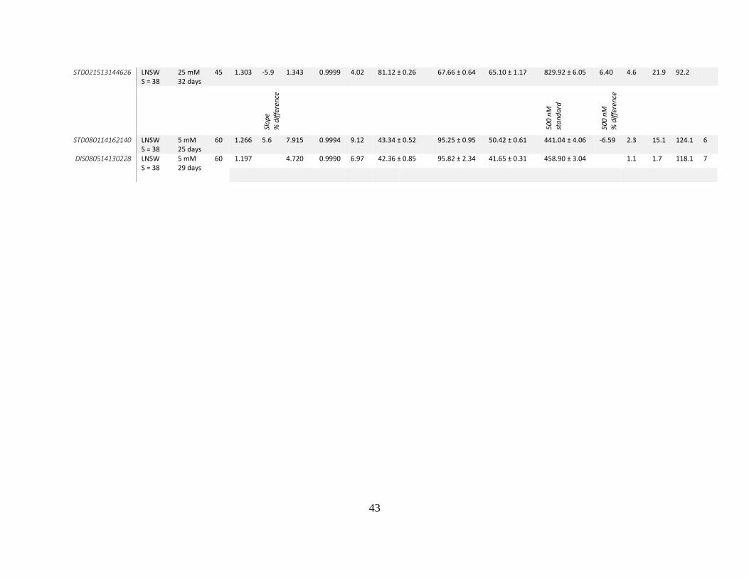
43

STD021513144626 LNSW S = 38

25 mM 32 days

45 1.303 -5.9 1.343 0.9999 4.02 81.12 ± 0.26 67.66 ± 0.64 65.10 ± 1.17 829.92 ± 6.05 6.40 4.6 21.9 92.2

Slo

pe

% d

iffe

ren

ce

50

0 n

M

sta

nd

ard

50

0 n

M

% d

iffe

ren

ce

STD080114162140 LNSW S = 38

5 mM 25 days

60 1.266 5.6 7.915 0.9994 9.12 43.34 ± 0.52 95.25 ± 0.95 50.42 ± 0.61 441.04 ± 4.06 -6.59 2.3 15.1 124.1 6

DIS080514130228 LNSW S = 38

5 mM 29 days

60 1.197 4.720 0.9990 6.97 42.36 ± 0.85 95.82 ± 2.34 41.65 ± 0.31 458.90 ± 3.04 1.1 1.7 118.1 7

the development of a fluorescence-based reverse flow

Documents