The Development and Applications of a

Numerical Method for Compressible Vorticity Confinement

in Vortex-Dominant Flows

Guangchu Hu

Dissertation submitted to the faculty of the Virginia Polytechnic Institute and State University

in partial fulfillment of the requirements for the degree of

Doctor of Philosophy in

Aerospace Engineering

Bernard Grossman, Chairman

John Steinhoff Robert W. Walters

William H. Mason William Devenport

June 2001 Blacksburg, Virginia

Keywords: Vorticity Confinement, CFD, Vortex-dominant flows

Copyright 2001, Guangchu Hu

ii

The Development and Applications of a Numerical Method for Compressible Vorticity Confinement (CVC) in Vortex- Dominant Flows

by

Guangchu Hu

Committee Chairman: Bernard Grossman Aerospace Engineering

(ABSTRACT)

An accurate and efficient numerical method for Compressible Vorticity Confinement (CVC) was

developed. The methodology follows from Steinhoff’s vorticity confinement approach that was

developed for incompressible flows. In this research, the extension of this approach to compressible flows

has been developed by adding a vorticity confinement term as a “body force” into the governing

compressible flow equations. This vorticity confinement term tends to cancel the numerical dissipative

errors inherently related to the numerical discretization in regions of strong vorticity gradients.

The accuracy, reliability, efficiency and robustness of this method were investigated using two methods.

One approach is directly applying the CVC method to several real engineering problems involving

complex vortex structures and assessing the accuracy by comparison with existing experimental data and

with other computational techniques. Examples considered include supersonic conical flows over delta

wings, shock-bubble and shock-vortex interactions, the turbulent flow around a square cylinder and the

turbulent flow past a surface-mounted 3D cube in a channel floor. A second approach for evaluating the

effectiveness of the CVC method is by solving simplified “model problems” and comparing with exact

solutions. Problems that we have considered are a two-dimensional supersonic shear layer, flow over a

flat plate and a two-dimensional vortex moving in a uniform stream.

The effectiveness of the compressible confinement method for flows with shock waves and vortices was

evaluated on several complex flow applications. The supersonic flow over a delta wing at high angle of

attack produces a leeward vortex separated from the wing and cross flow, as well as bow shock waves.

iii

The vorticity confinement solutions compare very favorably with experimental data and with other

calculations performed on dense, locally refined grids. Other cases evaluated include isolated shock-

bubble and shock-vortex interactions. The resulting complex, unsteady flow structures compare very

favorably with experimental data and computations using higher-order methods and highly adaptive

meshes.

Two cases involving massive flow separation were considered. First the two-dimensional flow over a

square cylinder was considered. The CVC method was applied to this problem using the confinement

term added to the inviscid formulation, but with the no-slip condition enforced. This produced an

unsteady separated flow that agreed well with experimental data and existing LES and RANS

calculations. The next case described is the flow over a cubic protuberance on the floor of a channel. This

flow field has a very complex flow structure involving a horseshoe vortex, a primary separation vortex

and secondary corner vortices. The computational flow structures and velocity profiles were in good

agreement with time-averaged values of the experimental data and with LES simulations, even though

the confinement approach utilized more than a factor of 50 fewer cells (about 20,000 compared to over 1

million).

In order to better understand the applicability and limitations of the vorticity confinement, particularly the

compressible formulation, we have considered several simple model problems. Classical accuracy has

been evaluated using a supersonic shear layer problem computed on several grids and over a range of

values of confinement parameter. The flow over a flat plate was utilized to study how vorticity

confinement can serve as a crude turbulent boundary layer model. Then we utilized numerical

experiments with a single vortex in order to evaluate a number of consistency issues related to the

numerical implementation of compressible confinement.

iv

Dedication

In Memoriam

Shengying Yang 1920-1984 Youcai Yang 1930-1998

In hope of their children and grandchildren will live in great happiness

To the most important people in my life:

my father, Sigao Hu,

and my wife, Xulian Yang

v

Acknowledgements

The author is greatly indebted to Dr. Bernard Grossman for his guidance and financial support over the

last four years. I have to thank Dr. John Steinhoff for his excellent ideas that inspired my thinking of the

essential mechanisms of vorticity confinement. I appreciate Dr. Mason who always had a friendly attitude

towards me when I asked questions; he taught me configuration aerodynamics and made me clearly

understand the differences between the leading-edge separation of the traditional wings and delta wings. I

would like to acknowledge the useful advice of Dr. Walters for accuracy analysis of vorticity

confinement method despite his busy schedule. I have enjoyed interacting with Dr. Devenport whose

cheerful attitude and good advice for the comparison of the present numerical solutions with analytical

solutions deserves a lot of thanks.

I owe a lot to Dr. Yonghu Wenren from Flow Analysis Inc. for his help and many useful discussions

about vorticity confinement. This work would not have been possible without the financial support from

Flow Analysis Inc. over the last one and half years. I wish to acknowledge my good teacher Dr. Kyle

Anderson from NASA Langley. He taught me CFD and gave me a lot of CFD knowledge. He always

treated me like a friend and answered what I asked both in class and after class through emails. I have to

thank Dr. Ribbens, Dr. Watson and Dr. Santos in the Computer Science Department at Virginia Tech for

teaching me parallel algorithms and parallel implementations. I received many benefits from their courses.

I would like to thank my family for always supporting me through good and difficult times in the past

years. My father Sigao Hu, my mother Shengying Yang and my brother Guangyi Hu constantly urged

me on to study hard. My sisters Guangrong Hu and Shuhua Hu, my brother-in-law Zihe Cheng and

Xinglen Qiao gave me a lot of financial support during difficult times. My wife Xulian Yang encouraged

me to finish my Ph.D. despite the obstacles on my road. My 13 year old son Zongyang Hu helped me a

lot by typing the draft and drawing a part of the plots for this dissertation; he always kept me smiling

when I faced difficulties.

vi

I have to thank my good friend Dr. Philippe-Andre Tetrault in Pratt & Whitney and my good friend Mr.

Hongman Kim (hoping to be a Doctor soon) for their help and good discussions over the years. And big

thanks go to Ms. Foushee, Ms. Williams and Ms. Coe in the AOE Department. Many thanks go to Ms.

Ghaderi and Mr. Brizee in the Virginia Tech Writing Center. They read and corrected the first draft of

this dissertation and gave me many tips of scientific writing. Without their help I would not have finished

this dissertation.

vii

Contents

1 Introduction 1 1.1 The Background of the Present Study………………………...…………….……………………1

1.2 Current Status of CFD in Calculation of Complex Vortex-Dominant Flows….……………..……5

1.3 Incompressible Vorticity Confinement (IVC)……………….…………………………………...8

1.4 Present Proposed Method for Compressible Vorticity Confinement (CVC)

for Complex Vortex-Dominant Flows………………………………………….………………..9

2 Formulation for Compressible Vorticity Confinement (CVC) 11 2.1 Incompressible Vorticity Confinement (IVC)……………………..…………………………….11

2.2 The Formulation for Compressible Vorticity Confinement (CVC)…..……….………………….13

2.3 Numerical Formulation…………………………………………………….…………………...17

2.4 Artificial Dissipation Models…………………………………………………………….….…..18

2.4.1 Scalar Dissipation Model (SDM) with Second-order and Fourth-order Difference ………...18

2.4.2 Matrix Dissipation Model (MDM (1)) with Second-order and Fourth-order Difference…….19

2.4.3 Matrix Dissipation Model (MDM (2)) with Second-order Difference and Linear or

Parabolic Interpolations for Primitive Variables……………………………………………22

2.4.4 Boundary Conditions for MDM (1)….…………..…………………………………………23

2.5 Matrix Compressible Vorticity Confinement Model (MCVC)…………………………………..25

2.6 The Choice of the Values of the Free Parameters ……………………………………………….27

3 Vortical Solutions of the Conical Euler Equations 28 3.1 Introduction………………………………………………………….….……………………...28

3.2 Governing Equations……………………………………….…………………………………..30

3.3 Vorticity Confinement Procedure………………………………………...……….…………….32

3.4 Solution Procedure…………………………………...……………………….………………...36

3.4.1 Grid Generation……………………………………………………….…………………37

3.4.2 Finite Volume Formulation………………………………………………………………38

3.4.3 Boundary Conditions…………………………………………………………………….41

3.5 Numerical Results for Conical Euler Equations……...…….………….………………………...42

3.5.1 Topology of the Conical Flows…………………………………………………………..44

3.5.2 Pressure Coefficient Profile…………………………………………….………………...45

viii

4 Numerical Simulations of Shock-Bubble and Shock-Vortex Interaction 53 4.1 Overview for Previous Studies in Shock-Bubble and Shock-Vortex Interaction..………....….…..53

4.2 Present Studies for Shock-Bubble Interaction..………………………………………...…….….54

4.3 Present Studies for Shock-Vortex Interaction..……………………………………...………..….59

4.4 Conclusion…………………………………………………………………………...……..….63

5 Calculations of Flows past Bluff Bodies 68 5.1 Introduction………………………………………………………………….………………...68

5.2 Calculation of a Flow past a 2D Square Cylinder.……………. ………………………………...69

5.3 Calculation of a Flow Over a Surface-Mounted Cube in a Plate Channel………………………..78

5.4 Conclusion.………………...…………………………………………....……………………..92

6 Parallel Computation for the Flow past a 3D Surface-Mounted

Cube Using Domain- Decomposition Algorithms 94 6.1 Introduction...……………………………………………………..………….………………...94

6.2 Computer Requirements………………………………………….……………………………95

6.3 Parallel Algorithms…………………………………………………..……….…………….…..95

6.3.1 Domain Decomposition Algorithm Using One-To-One Scheme ….………………………96

6.3.2 Domain Decomposition Using Pipeline Scheme…..…………………….………………...97

6.3.3 Synchronization………………………………………..…………………………………97

6.3.4 Load Balancing………………………………………….………………………………..98

6.4 Implementation Issues……….………..………………………….…………………………….98

6.5 Numerical Experiment Results and Analyses…....…………………………….………………..99

6.5.1 Speed Up and Efficiency vs. Scheme and Synchronization...….………….……………….100

6.5.2 Efficiency vs. Load Balancing…….……………………………………………………...100

6.5.3 Performance in Term of CPU Time………………………...…………………………….101

6.6 Conclusion……………….………………………………..……………… …………………101

7 Fundamental Properties of Compressible Vorticity Confinement (CVC) 104 7.1 Turbulent Boundary Layer Over a Flat Plate……..…………………….………………………104

7.2 Supersonic Shear Layer……………………………………………………….………………111

7.3 A Vortex Moving with a Uniform Free Stream………………………………………………..115

8 Summary and Conclusions 127

Bibliography 132

ix

Appendix A Characteristic Matrix and Dissipation Models 137

Appendix B Cross-flow Vorticity and Governing Equations in Conical Coordinates 141

Appendix C Analytical Solution and Initial Condition of a Moving Vortex

with a Uniform Stream 147

Vita 152

x

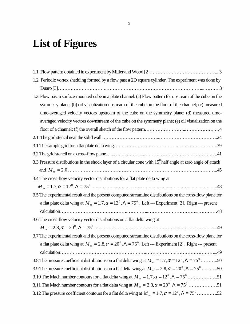
List of Figures

1.1 Flow pattern obtained in experiment by Miller and Wood [2]……………………………………...3

1.2 Periodic vortex shedding formed by a flow past a 2D square cylinder. The experiment was done by

Duaro [3]………………………….……………………………………………………...……….3

1.3 Flow past a surface-mounted cube in a plate channel. (a) Flow pattern for upstream of the cube on the

symmetry plane; (b) oil visualization upstream of the cube on the floor of the channel; (c) measured

time-averaged velocity vectors upstream of the cube on the symmetry plane; (d) measured time-

averaged velocity vectors downstream of the cube on the symmetry plane; (e) oil visualization on the

floor of a channel; (f) the overall sketch of the flow pattern……………………..……………….…4

2.1 The grid stencil near the solid wall..………………….…………..……………………………….24

3.1 The sample grid for a flat plate delta wing………………………………….……………………..39

3.2 The grid stencil on a cross-flow plane…...……………......……….……………………………….41

3.3 Pressure distributions in the shock layer of a circular cone with 150 half angle at zero angle of attack and 0.2=∞M …………………………………………………………………………………..45

3.4 The cross-flow velocity vector distributions for a flat plate delta wing at

00 75,12,7.1 =Λ==∞ αM …..………………………………….…...………………………….48

3.5 The experimental result and the present computed streamline distributions on the cross-flow plane for

a flat plate delta wing at 00 75,12,7.1 =Λ==∞ αM . Left --- Experiment [2]. Right --- present

calculation…………………………………….…………..…………………………...…………48

3.6 The cross-flow velocity vector distributions on a flat delta wing at

00 75,20,8.2 =Λ==∞ αM …………………………….………………………….…………...49

3.7 The experimental result and the present computed streamline distributions on the cross-flow plane for

a flat plate delta wing at 00 75,20,8.2 =Λ==∞ αM . Left --- Experiment [2]. Right --- present

calculation……………………………………………….…….………….……………………...49

3.8 The pressure coefficient distributions on a flat delta wing at 00 75,12,7.1 =Λ==∞ αM ………..50

3.9 The pressure coefficient distributions on a flat delta wing at 00 75,20,8.2 =Λ==∞ αM ……….50

3.10 The Mach number contours for a flat delta wing at 00 75,12,7.1 =Λ==∞ αM ……………….51

3.11 The Mach number contours for a flat delta wing at 00 75,20,8.2 =Λ==∞ αM ………………51

3.12 The pressure coefficient contours for a flat delta wing at 00 75,12,7.1 =Λ==∞ αM ………….52

xi

3.13 The pressure coefficient contours for a flat delta wing at 00 75,20,8.2 =Λ==∞ αM …………..52 4.1 The comparisons of density contours at (a) st µ123= , (b) st µ373= , (c) st µ573= ,

(d) st µ773= . Left side --- CVC. Right side --- Experiment [10]...…………………………..…...56

4.2 The comparisons of density contours at (a) st µ123= , (b) st µ373= , (c) st µ573= ,

(d) st µ773= . Left side --- CVC. Right side --- FCT [9]…………………………………………57

4.3 The comparisons of density contours at (a) st µ123= , (b) st µ373= , (c) st µ573= ,

(d) st µ773= . Left side --- CVC. Right side --- Adaptive Unstructured Algorithm [8] …………...58

4.4 A moving shock over a point vortex…………………………….………..……………………….61 4.5 The density contours at 421 sµ …………………………………………….……………………..61

4.6 The density contours at 0 - 421 sµ . (a, A) t = 0 sµ ; (b, B) t = 50 sµ ; (c, C) t = 70 sµ ;

(d, D) t = 90 sµ ; (e, E) t = 110 sµ ; (f, F) t = 157 sµ ; (g, G) t = 203 sµ ; (h, H) t = 421 sµ .

a ~ h ---- CVC. A ~ H ---- adaptive unstructured algorithm by Povitsky et al.…………...………..62

4.7 The comparison of the grids. (a), (e) the grid layout before and after interaction, unstructured adaptive

grid [8]; (b), (f) the grid layout before and after interaction of the present study, 200x50; (c), (g) the

grid layout before and after interaction of the present study , 300x100; (d), (h) the grid layout before

and after interaction of the present study, 600x200………………………………………………..65 4.8 The comparison of density contours at time 157 sµ on different grids. (a) unstructured adaptive grid

[8]; (b) regular Cartesian grid of the present study 600x200; (c) regular Cartesian grid of the present

study 300x100; (d) regular Cartesian grid of the present study 200x50……..……..……………….66 4.9 The density contours at (a) t = 90 sµ and (b) t = 157 for the grid 200x50 and E c = 0.4………….....67

5.1 Streamline distributions at three phases and time variation of pressure and lift coefficient for a flow

past a 2D square cylinder; a, e – experiments of Lyn et al. [49,50], b -- RANS-RSM of Franke et al.

[14], c -- LES-UKAHY2 of Rodi [13], d, f – CVC..….…………….……………………………...73

5.2 Time averge-velocity U along the centerline of a 2D square cylinder…………………….………...76

5.3 The mean pressure on the surface of a 2D square cylinder………………………………………....77

5.4 The grid layout on the symmetry plane of a cube……………………....………………………….78

5.5 The comparisons of the streamline distributions on the symmetry plane and on the floor of the

channel…………………………………………………...……………………………..……….83

5.6 The comparisons between CVC and the LES calculation [57] for the streamline distributions on the

plane parallel to the back face at 0.1step size of the cube dimension……………..………………..84

5.7 Comparison of the streamline distributions with and without CVC on the plane near the floor of the

channel. Grid 32x24x24………………………………………………………………………...85

xii

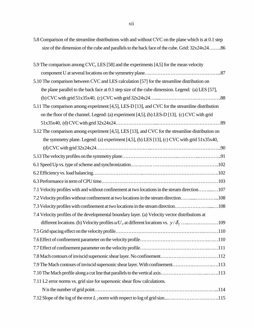
5.8 Comparison of the streamline distributions with and without CVC on the plane which is at 0.1 step

size of the dimension of the cube and parallels to the back face of the cube. Grid: 32x24x24……..86

5.9 The comparison among CVC, LES [58] and the experiments [4,5] for the mean velocity

component U at several locations on the symmetry plane………………………………………...87

5.10 The comparison between CVC and LES calculation [57] for the streamline distribution on

the plane parallel to the back face at 0.1 step size of the cube dimension. Legend: (a) LES [57],

(b) CVC with grid 51x35x40, (c) CVC with grid 32x24x24….....………………………………..88

5.11 The comparison among experiment [4,5], LES-D [13], and CVC for the streamline distribution

on the floor of the channel. Legend: (a) experiment [4,5], (b) LES-D [13], (c) CVC with grid

51x35x40, (d) CVC with grid 32x24x24……………………...…………………………………89

5.12 The comparison among experiment [4,5], LES [13], and CVC for the streamline distribution on

the symmetry plane. Legend: (a) experiment [4,5], (b) LES [13], (c) CVC with grid 51x35x40,

(d) CVC with grid 32x24x24……………………………..……………………………………..90

5.13 The velocity profiles on the symmetry plane……………………………..…………..…………..91

6.1 Speed Up vs. type of scheme and synchronization…….……. …………………………………..102

6.2 Efficiency vs. load balancing…………………………..….…………………………………….102

6.3 Performance in term of CPU time……………………….………………………………………103

7.1 Velocity profiles with and without confinement at two locations in the stream direction…….....…107

7.2 Velocity profiles without confinement at two locations in the stream direction…….....…………...108

7.3 Velocity profiles with confinement at two locations in the stream direction………………….....…108

7.4 Velocity profiles of the developmental boundary layer. (a) Velocity vector distributions at different locations. (b) Velocity profiles u/U e at different locations vs. Ty δ/ …...………………109

7.5 Grid spacing effect on the velocity profile……………………………………………….………110

7.6 Effect of confinement parameter on the velocity profile…………………………………….……110

7.7 Effect of confinement parameter on the velocity profile…………………………………….……111

7.8 Mach contours of inviscid supersonic shear layer. No confinement………………………………112

7.9 The Mach contours of inviscid supersonic shear layer. With confinement…………………….….113

7.10 The Mach profile along a cut line that parallels to the vertical axis…………………….…..…….113

7.11 L2 error norms vs. grid size for supersonic shear flow calculations.

N is the number of grid point…………………………………………………………………...114

7.12 Slope of the log of the error L 2 norm with respect to log of grid size...….……………………….115

xiii

7.13 Sample grid for calculation of a moving vortex in uniform compressible flow…………………..117

7.14 Vorticity contours for a vortex moving with free stream after one cycle. No confinement…….…119

7.15 Vorticity contours for a vortex moving with a free stream after ten cycles. No confinement……..119

7.16 Vorticity contours for a vortex moving with a free stream after one cycle. With confinement…....120

7.17 Vorticity contours for a vortex moving with a free stream after 10 cycles. With confinement……120

7.18 Vorticity profile along a vertical slice taken through the center of the vortex. Fine

grid 100x100………………………………………………………………………………......121

7.19 Vorticity profile along a vertical slice taken through the center of the vortex. Coarse

grid 13x13.…………………………………………………………………………………….121

7.20 The average total temperature versus time iterations for different vorticity confinement

procedures for a moving vortex………………………………………………………………..124

7.21 The velocity profile at 2L/3 for different vorticity confinement procedures…………….………..125

7.22 The average total temperature versus time iterations for different vorticity confinement

procedures applied to the flow over a flat plate…………………………………………………126

1

Chapter 1 Introduction In this chapter, the background of the present study will be stated, the difficulties will be described from

the viewpoint of CFD and the significance will be noted in the design and analysis for fluid dynamics and

aerodynamics. This will be followed with a prentation of the current status of CFD in complex vortex-

dominant flows along with a discussion of the present proposed Compressible Vorticity Confinement

(CVC) method. Finally, the organization of the dissertation will be given.

1.1 The Background of the Present Study

In the last three decades, CFD has been developed as a standard design and analysis tool in fluid

dynamics and aerodynamics. CFD can shorten the time and lower the cost required to obtain

aerodynamic flow simulations necessary for the design of new structures or aerospace vehicles.

According to Paul E. Rubbert [1], Boeing completed upgrading its 737 family of airplanes in response to

changing customer needs with the aid of fast, CFD-based design processes. It is well known that CFD

can predict the behavior of attached flows, and as the speed and memory capability of the computer are

increased, CFD researchers can perform flow simulations that are either impractical or impossible to

obtain in wind tunnels or other ground based experimental test facilities. However, despite many recent

advances, it is difficult for CFD researchers to simulate complex separated (vortex-dominant) flows,

which may occur at high angles of attack or with bluff bodies. In those situations, the flows are turbulent,

and may involve complicated multiple separations, shock-vortex interactions, vortex shedding, vortex-

vortex interaction, vortex merging, impingement, reattachment, recirculation and bimodal behavior.

Figure 1.1 shows the flow patterns in an experiment [2] when a supersonic flow with free stream Mach

number 1.7 passes a flat delta wing at angle of attack 13 degrees. Flow separation occurs at the leading

2

edges, resulting in large primary vortices on the lee-side with small viscous-induced secondary ones

beneath them; cross-flow shocks are formed and interact with vortices to yield very complex vortical

motions. Figure 1.2 presents a flow pattern formed by a flow over a 2D square cylinder at a high

Reynolds number, according to the experiment done by Duaro et al. [3]. The separation occurs at the

frontal corner with steep streamline curvature, forming recirculation behind the model and periodic vortex

shedding. Figure 1.3 shows the flow patterns formed by a flow passing a surface-mounted cube in a plate

channel according to the experiment done by Larousse, Martinuzzi and Tropea [4,5]. Line A in

Figure1.3b corresponds to the primary separation caused by the strong adverse pressure gradient imposed

by the cube in this region; the horseshoe vortex is clearly recognized in the velocity vector field shown in

Figure 1.3c, which corresponds to the line B in Figure 1.3b. The bimodal behavior is shown in the region

between the primary separation and the horseshoe vortex. In addition to the primary and secondary

separation in front of the cube, the flow separates at the upper leading edge as well. Figure 1.3d shows

two mean recirculation regions: one is over the top; the other is behind the cube. Two corner vortices are

formed behind the cube on the floor of the channel and indicated in Figure1.3e. The overall flow pattern

was sketched and shown in Figure1.3f [4,5].

Understanding the mechanism of complex vortex-dominant flows is of great importance for designing

good and safe vehicles and structures. Many fighter aircraft incorporate a delta-wing lifting surface. When

they fly at high angles of attack and supersonic speeds, the flow will be separated at the leading edge of

the wings, leading to leading-edge vortices with inboard cross-flow shock waves. This flow environment

may be unsteady and introduces many interesting nonlinear aerodynamic behaviors that may be

beneficial or detrimental to the aircraft performance. A flow over a bluff body such as a building, a bridge,

an automobile, etc., occasionally will produce periodic vortex shedding. Generally speaking, periodic

vortex shedding will cause dynamic loading on the bodies, which, in extreme cases, may cause

catastrophic failures.

3

Figure 1.1: Flow pattern obtained in experiment by Miller and Wood [2].

Figure 1.2: Periodic vortex shedding formed by a flow past a 2D square cylinder. The experiment was

done by Duaro [3].

4

Figure 1.3: Flow past a surface-mounted cube in a plate channel. (a) Flow pattern for upstream of the

cube on the symmetry plane; (b) oil visualization upstream of the cube on the floor of the channel; (c)

measured time-averaged velocity vectors upstream of the cube on the symmetry plane; (d) measured

time-averaged velocity vectors downstream of the cube on the symmetry plane; (e) oil visualization on

the floor of the channel; (f) the overall sketch of the flow pattern.

Legend: S --- saddle; N --- node; ’ --- half saddle or node; * --- point viewed perpendicularly to the wall.

Subscripts: s --- separation; a --- attachment.

The experiment was done by Larousse, Martinuzzi and Tropea [4,5].

5

1.2 Current Status of CFD in Calculation of Complex Vortex-Dominant Flows

In general, vortex-dominant flows may be solved using two CFD approaches. One approach directly

solves the Navier-Stokes (NS) equations plus the continuity equation without adding any model such as

the Direct Numerical Simulation (DNS); the other approach solves Euler or NS equations plus the

continuity equation with some models such as solving RANS equations with various turbulence models

or LES models. The current status of CFD in the calculations of complex vortex-dominant flows can be

summarized as follows:

1.2.1 Solving Euler or NS Equations with the Continuity Equation Using Higher Order Discretization, a Fine Grid or an Adaptive Grid (Structured or Unstructured). Euler equations are

used when viscous effects can be ignored; NS equations are used when viscous effects are considered. As

we know, higher order discretization increases CPU loading, fine grid wastes memory storage, and

adaptive procedures have a lot of complex logic controls. All these procedures are used for one objective,

that is, to decrease the dissipation/dispersion errors inherently related to the numerical discretization.

Some example of complex discretization include a fifth order discretization of NS equations with a fine

regular grids which was used to solve the problem involving vortices impinging on an airfoil by Rai et al.

[6]. A steady vortex shed at the tip of a straight wing was studied by Strawn [7] using an unstructured

adaptive grid. Interaction between a vortex and a propagating shock wave was calculated by Povitsky and

Ofengeim with an adaptive unstructured scheme [8]. Yang et al. simulated the interaction between a

moving shock wave with a circular light gas bubble in a channel with a finite width using a higher-order

Flux-Corrected-Transport (FCT) scheme [9], but seemed not to get good agreement with the experiment

[10]. Powell [11] embedded extra grid points in the vortical regions in the calculation of flows over plate

delta wings, but still had difficulty in capturing the primary vortices without having them spread over a

larger region than those measured in experiments. Furthermore, generally speaking, in current CFD

methods, the calculated peak of the vorticity in the core region of the vortex is typically smaller than that

measured in the experiment.

6

Shu [12] used fifth order finite difference WENO scheme to simulate a vortex periodically moving along

one of the diagonals of a square domain with dimension of 10 units along with a uniform mesh of 80x80

points. In addition, the same problem was simulated using a second order finite difference MUSCL type

TVD scheme. At time t = 10, both schemes obtained good agreement with the “exact” solution; but at

time t = 100, the solution with the second order scheme shows too much dissipation in the core region of

the vortex, the solution with the fifth order scheme still has good agreement with the “exact” solution.

However, Shu reported in Ref. [12]: “the CPU time of a fifth order finite difference WENO scheme is

roughly 3 to 8 times more than that of a second order TVD scheme (depending on the specific forms of

the schemes and time discretization)”.

1.2.2 Solving RANS Equations with Various Turbulence Models Which Include Algebraic Models, One-Equation Models, Two-Equation Models and Second-Order Closure Models. Until now there

has been no universally acceptable turbulence model that can provide uniformly good results for

engineering problems with separated flows. Algebraic models are simple to use, but are quite unreliable

for separation flows because of the Boussinesq and “equilibrium” approximations implicit in these

models. One-equation models have achieved closer agreement with experimental measurements for a

limited number of separated flows than is possible with algebraic models, but the length scale for each

new application needs to be specified. The ε−k model is the most widely used in the family of two-

equation models; unfortunately, it is inaccurate for flows with adverse pressure gradients, separation and

recirculation. Sometimes modified ε−k models yield better results for limited classes of problems, such

as the Low-Reynold-Number modification, Two-Layer (TL) modification and Kato-Launder (KL)

modification. Generally speaking, the Reynold-Stress-Model (RSM) predicts better results than the

standard ε−k model does, but it seems not to be promising when used in massively separated flows

over bluff bodies. The ω−k model is very accurate for 2D boundary layers with variable pressure

gradients (both adverse and favorable), but this model is very sensitive to the free stream boundary

conditions for free shear flows. Rodi et al. [13-15] simulated the flows over a 2D square cylinder and a

3D surface-mounted cube in a channel by solving RANS with various turbulence models. They claimed

that the standard ε−k model completely failed to predict the flows over bluff bodies because it

produced very large turbulent energy in the front stagnation regions and very large recirculation regions behind the bodies. The ε−k model with KL modification )( ε−− kKL and the wall function solved the

problem with very large turbulent energy in the front stagnation regions, but still overestimated the length of the reverse flow regions. RSM with TL modification )( RSMTL − predicted too short separation

7

zones behind the bodies. It appears that all two-equation models are inaccurate for the flows around

surfaces with large curvatures, separations, sudden change in mean strain rate, rotation, vortex shedding,

and 3D unsteady motions.

1.2.3 Direct Numerical Simulation (DNS). Solves the exact time-dependent NS equations with the

continuity equation under the assumption of no significant numerical and other form of errors. In

principle, the grid must be fine enough to resolve the smallest eddies whose size is of the order of the

Kolmogorov length scale, and the computational time step should be of the same order of the

Kolmogorov time scale. Kim et al. [16] performed a DNS for a channel flow with Reynolds number

6,000 (based on H, the height of the channel) with grid points 2 and 4 million. The CPU time on Cray

X/MP for the finer grid is 40 seconds per time step. 250 CPU hours was required in a run for a total time

τuHt /5= , where τu is the friction velocity at the wall of the channel, ρττ /wu = . Speziale [17]

noted that a DNS of turbulent pipe flow at Reynolds number 500,000 would require a computer 10

million times faster than a Cray Y/MP. In conclusion, there is a very long way to go for DNS to be a

practical tool in the CFD community.

1.2.4 Large Eddy Simulation (LES). Similar to DNS, solves the complete time-dependent NS

equations with the continuity equation, but on a grid whose size is much larger than that used in DNS.

The large-scale eddies whose size is larger than the order of grid size are resolved; the small eddies whose

size is smaller than the order of grid size are filtered out and are modeled, usually using a Smagrorinsky

or a Dynamic model. Rodi reported in Ref. [13] the LES calculations for a flow past a 2D square cylinder

and a flow over a surface-mounted cube in a plate channel using CPU time 73 hours and 160 hours,

respectively, on the SNI S600/20 vector computer. Although LES is more economical than DNS

(typically, requiring 5-10 percent of the CPU time required for DNS), it still requires very large computer

resources. Rodi reviewed the LES calculations for the flow past a 2D square cylinder and concluded in

his paper [13]: “it was found that none of the LES results are uniformly good and entirely satisfactory and

there were large differences between the individual calculations which are difficult to explain.”

1.2.5 Lagrangian Methods. These methods treat flows with vortical motions by assigning vorticity or

circulation to individual markers that are fixed in the flow field or convect with fluids. Leonard reviewed

vortex methods with Lagrangian approaches for flow simulations in Ref. [18]. Methods that were

8

described included the point vortex method, the vortex blob method, and the contour dynamics method

for two-dimensional flows, and the vortex filament method and its application to the aircraft-trailing

vortices in three-dimensional flows. Furthermore, Leonard discussed the details of the vortex-in-cell

methods in which the Lagrangian treatment of the vorticity field is retained, but the velocity field is solved

on a fixed Eulerian mesh. As a result, the very high cost of the Biot - Savart integration is avoided when

many vortex elements are used. In addition, “vortex lattice” or “vortex blob” techniques [19] and the

“vortex embedding” technique [20] were employed to entail representation of vortex sheets or vortex

filaments over surfaces or lines defined by markers in vortex dominated flows. Unfortunately, the

Largrangian approach lacks the generality of being used to solve complex vortex–dominant flow

problems, because in realistic engineering flows, vortex filaments may merge and reconnect, or boundary

layers may abruptly separate, shedding a convecting vortex. Sometimes, multiple sheets may be shed

from different places on the same surfaces and some may reattach. These complicated phenomena make

the specification of markers very difficult.

1.3 Incompressible Vorticity Confinement (IVC) IVC solves the incompressible Euler/NS equations plus the continuity equation with vorticity

confinement terms to try to remove the numerical dissipation inherently related to the numerical

discretization in vortical regions. For vortex dominated flows, because the vorticity confinement terms

take care of the numerical dissipation errors, very simple schemes can be used to discretize the governing

equations in order to save computing time. Vorticity confinement was proposed by Steinhoff and his

coworkers in Refs.[21-24] for computing flows with concentrated vorticity. This method was originally

applied to incompressible flows. Steinhoff and coworkers applied a velocity correction to the momentum

conservation equations and solved the incompressible NS equations for two- and three-dimension vortex

dominated flows [21,22]. The correction term is limited to the vortical regions and does not affect

nonvortical regions. Similar to shock capturing techniques, vorticity confinement treats vortical layers

without a detailed resolution of their internal structure. The confinement procedure is constructed in such

a way that it preserves certain conservation laws outside and integrated over the vortical regions. This

method can easily be incorporated into a standard Euler method on a fixed grid [23]. Applied to various

flows involving a concentrated vorticity, the vorticity confinement approach has proved capable of

treating thin vortical structures in complicated flows with massive separation using relatively coarse grids

9

[21-24]. Following the same anti-diffusive convection idea as in vorticity confinement, Steinhoff et al.

[25] have developed a new confinement procedure for short acoustic pulses. A “Pressure Confinement”

convects the pressure wave back towards the center of a propagating pulse and balances a numerical

diffusion of a basic traditional solver.

1.4 Present Proposed Method for Compressible Vorticity Confinement (CVC) for Complex Vortex-Dominant Flows

CVC solves the exact time-dependent Euler equations with simple viscous boundary layer model

equations (Euler/BC) plus the continuity equation with vorticity confinement terms as a “body force” on

regular Cartesian grid. The governing equations are mass, momentum and energy conservation laws, so it

can handle compressible phenomena like shock-vortex interactions in supersonic and hypersonic flows.

IVC cannot do this because it solves incompressible Euler/BC equations with the continuity equation.

This method is called Compressible Vorticity Confinement (CVC), because it is constructed from the

compressible formulation. The viscosity effect is ignored in the rest of the dissertation, because most of

the real engineering problems have very large Reynolds numbers; the extension to NS equations is

straightforward. CVC can resolve the large-scale unsteady vortical motions like LES, but without

considering viscosity effect and subgrid-scale model. The problem is considered in another way by

adding the “body force” to try to remove the dissipation inherently related to numerical discretization in

vortical regions, decreasing numerical errors in the solution procedure, so that the weak and small-scale

vortical motions are not damped out by numerical dissipation. Furthermore, a very coarse grid can be

used for 3D complicated turbulent flows with massive separations; so only very small CPU time is

required compared to LES calculation. With the preliminary results of conical vortical flows on plate

delta wings, interaction of a moving shock wave with a light gas bubble and a light gas circular vortex,

flows past a 2D square cylinder and a 3D surface-mounted cube in a plate channel, we have almost

achieved our objective. The dissertation will be organized as follows:

Chapter 2 describes the CVC method constructed by using conservation laws and finite-volume cell-

centered discretization. Chapter 3 applies CVC to conical vortical flows over flat delta wings. We chose

conical vortical flows over flat delta wings as one of our applications because leading-edge vortex flows

in particular are of great interest to aerodynamicists. The lee-side vortices, when symmetry and stable, can

10

lead to beneficial high-lift situations; otherwise, they may lead to disaster. This kind of problem has a very

simple geometry with a flat plate delta wing at angles of attack, but can lead to extremely intricate and

intriguing flow topologies, producing a rich variety of leading-edge vortices and shock-vortex interaction

patterns; moreover, these complicated flow situations cannot be adequately handled by current CFD

methods.

Chapter 4 applies CVC to the interaction of a moving shock wave with a density inhomogeneity. We will

investigate a two-dimensional moving shock wave over a circular light-gas inhomogeneity both in the

form of a bubble and a circular vortex in a channel with a finite width. The pressure gradient formed by a

moving shock wave interacts with the density gradient at the edge of the inhomogeneity to produce

vorticity around the perimeter, and the structure rolls up into a pair of counter-rotating vortices. A

practical application of the shock-induced vortices is the rapid and efficient mixing of fuel and oxidizer in

a SCRAMJET combustion chamber.

Chapter 5 applies CVC to complex vortex-dominant flows over bluff bodies. We will study the flows

over a 2D square cylinder and a 3D surface-mounted cube in a plate channel. We chose these applications

to test CVC because the flows over bluff bodies involve impingement, multiple separations at different

places, recirculations, bimodal behaviors, corner and arch vortices, periodic vortex shedding and 3D

unsteady vortical motions. These flow phenomena are the most challenging in current CFD; no method

can provide uniformly good results for these flows.

In Chapter 6, we present the parallel computing implementation for the calculation of the flow past a 3D

surface-mounted cube and present the performance of this parallel calculation. Then in Chapter 7, we

present the fundamental properties of CVC, which includes the accuracy analysis and limitation

discussion for the CVC method. The dissertation ends with the summary and conclusions in Chapter 8.

11

Chapter 2 Formulation for Compressible Vorticity Confinement (CVC)

In this chapter we will first present the previous studies of vorticity confinement by Steinhoff and his

coworkers in the last decade. This is followed by the formulation for the CVC method, and finally we

will describe the numerical methods used in the present study.

2.1 Incompressible Vorticity Confinement (IVC)

The original vorticity confinement approach was designated for incompressible flows with thin

concentrated vorticity structures by Steinhoff and his coworkers [21-24]. This method is somewhat

similar to the shock capturing method. Thin vortical layers are treated without detailed resolution of their

internal structure in a way similar to shock capturing algorithms in which a shock is captured in 2-3 grid

cells without resolving the internal structure. The vorticity confinement term is built in such a way that

conservation laws are preserved outside and integrated over the vortical regions; it is non-zero only within

the vortical regions, and does not change the total vorticity or mass within those regions. This method can

be easily incorporated with standard Euler / “Navier-Stokes” solvers (Euler with turbulence models) on a

fixed grid. The core of the method is a velocity correction, applied locally, which prevents the vorticity

from degrading during its propagation due to the numerical diffusion.

Numerical implementation of the vorticity confinement for an incompressible flow includes 3 main steps

[26-28]:

1. Velocity convection based on momentum equations;

12

2. Velocity correction according to the vorticity confinement;

3. Solution of the pressure to mass conservation, as a conventional “split velocity” method [29].

Applied to incompressible flows, vorticity confinement has proven to be an efficient method. Some of the

details of the basic method are presented in Refs. [21-24]. The method involves adding a term to the

momentum equations. When these equations are discretized by finite difference methods, the modified

equations include truncation error, so we actually solve the modified equations. For incompressible flow

the original formulation of the vorticity confinement method of Steinhoff can be written as follows:

0=⋅∇ q , (2.1)

kqpqqtq r

rrr

r

εµρ +∇+∇−∇⋅−=∂∂ 2)/()( , (2.2)

where q is the velocity vector, ρ is density, p is pressure, and µ is a diffusion coefficient. In

Steinhoff’s formulation, the diffusion term is an artificial dissipation. The additional term k

ε is a vorticity confinement term; ε is a numerical coefficient that controls the size of the convecting vortical regions.

The confinement term has the form:

ω

×−= cnk ˆ , (2.3)

||)(|||)(|ˆ

ωω

∇∇−=cn , (2.4)

qrr ×∇=ω , (2.5)

where cn is a unit vector pointing away from the centroid of the vortical region and the term k

ε serves to

convect ω back towards the centroid as it diffuses away. This term is added to correct the diffusive error

in the momentum equations. A non-diffusive solution will be obtained when the vorticity confinement

and the numerical diffusion become balanced. Under this circumstance, the vorticity confinement

conserves momentum.

13

2.2 The Formulation for Compressible Vorticity Confinement (CVC)

Vorticity confinement has been proved to be an efficient method in conjunction with finite difference

schemes as a basic solver in incompressible flow. However, attempting to extend ICV to compressible

flows turns out to be not straightforward. A partial explanation of this could be that vorticity confinement

acts only on the velocity field and implicitly balances the diffusive error only in momentum equations. At

the same time, the velocity correction term works as an unbalanced source for the energy equation and

mass continuity equation for compressible flows. Traditional compressible solvers do not include a

mass/energy conservation step similar to the one in the “split-velocity” method used in incompressible

flows. As a result, there is no steady-state solution for the modified system of equations. For the time-

dependent problems, this error is practically negligible for low subsonic flow. But if we extend this

method directly to transonic and supersonic vortex-dominant flows, this error for time-dependent

problem will be large, and cannot be neglected, so we need a more consistent way to construct vorticity

confinement for compressible flows.

There have been several attempts to extend the vorticity confinement to compressible flows. Pevchin [30]

et al. developed a very complicated formulation based on flux splitting which was dependent upon the

grid orientation. Yee and Lee [31] attempted to use the incompressible vorticity confinement term

directly in the compressible momentum equations, and that produced an inconsistent formulation. In the

present work, we added the confinement term in a consistent way within a conservation law framework.

We have noted that the confinement term added to momentum equations in Steinhoff’s formulation may

be interpreted as a “body force”. We can then extend the approach to compressible conservation laws by

adding this “body force” to the integral momentum equations and rate of work done by the “body force”

to energy conservation law. This eliminates the inconsistencies due to directly extending the original

vorticity confinement just in momentum equations in incompressible flow to compressible flow; a non-

diffusion solution can be achieved even for time-dependent supersonic problems. A finite-volume

scheme with CVC then can be developed directly.

The integral conservation laws for mass, momentum and energy may be written for a control volume

fixed in space as follows:

14

0ˆ =⋅+∫ ∫ ∫ ∫ ∫ σρτρ dnVddtd

V S s

, (2.6)

τρσσρτρ dfdnpdnVVdVdtd

V bS sV S s ∫ ∫ ∫∫ ∫∫ ∫ ∫ ∫ ∫ +−=⋅+

ˆ)ˆ( , (2.7)

∫ ∫ ∫∫ ∫∫ ∫∫ ∫ ∫ ⋅+⋅−=⋅+V bS ssS OV O dfVdnVpdnVede

dtd τρσσρτρ

ˆˆ , (2.8)

where bf

is a “body force” per unit mass (acceleration), which serves to try to balance the numerical

diffusion inherently related to numerical discretization and conserve momentum in vortical regions. We

have presented the form of the equations for inviscid flows here, but the extension to viscous flows is

straightforward.

Now, we define the “body force” term bf

as follows:

ω

×−= ccb nEf ˆ , (2.9)

where cn has the definition in Eq. (2.4), and ω is the vorticity vector defined in Eq. (2.5). E c is a

positive vorticity confinement parameter. Eqs. (2.6)-(2.8) are used directly to develop a finite-volume

scheme. After manipulating Eqs. (2.6)-(2.8) by using Gauss's divergence theorem, we can rewrite

Eqs. (2.6)-(2.8) in Cartesian coordinates as follows:

SzH

yG

xF

tQ =

∂∂+

∂∂+

∂∂+

∂∂ , (2.10)

where

+=

+=

+=

=

0

2

0

2

0

2

,,,

whpw

vwuww

H

vhvw

pvvuv

G

uhuwuv

puu

F

ewvu

Q

O ρρρρρ

ρρ

ρρρ

ρρρ

ρρ

ρρρρρ

, (2.11)

15

where e 0 is the total energy in unit mass, 0h is the stagnation enthalpy, p is the pressure, S is the vorticity

confinement term. They are defined as follows:

ρ/00 peh += ,

]2/)([)1( 2220 wvuep ++−−= ργ , (2.12)

⋅⋅⋅⋅

=

Vfkfjfif

S

b

b

b

b

rr

r

r

r

ρρρρ

ˆˆˆ

0

,

where ρ is density, p is pressure, (u, v, w) is the velocity component in (x, y, z) direction respectively,

and )ˆ,ˆ,ˆ( kji is the unit vector in (x, y, z) direction respectively. For convenience, let's define a scalar variable φ as the magnitude of the vorticity vector ω as follows:

222zyx ωωωωφ ++== . (2.13)

So, in Cartesian coordinates

kjin zsysxscˆˆˆˆ φφφ

φφ ++=

∇∇−= , (2.14)

where

zyx

xxs 222

φφφ

φφ++

= ,

zyx

yys 222

φφφ

φφ

++= , (2.15)

zyx

zzs 222

φφφ

φφ++

= .

16

Now we get the expression of bf

kfjfifkji

EnEf bzbybx

zyx

zsysxscccbˆˆˆ

ˆˆˆ

ˆ ++=

−=×−=ωωωφφφω

, (2.16)

where

)( zsyyszcbx Ef φωφω −−= ,

)( xszzsxcby Ef φωφω −−= , (2.17)

)( ysxxsycbz Ef φωφω −−= ,

and

.

,

,

yu

xv

xw

zu

zv

yw

z

y

x

∂∂−

∂∂=

∂∂−

∂∂=

∂∂−

∂∂=

ω

ω

ω

(2.18)

Finally, the vorticity confinement term in a compressible flow can be expressed as follows:

−+−+−−−−−−−−

=

++

=

)]()()([)()()(

0

)(

0

ysxxsyxszzsxzsyyszc

ysxxsyc

xszzsxc

zsyyszc

bzbybx

bz

by

bx

wvuEEEE

wfvfuffff

S

φωφωφωφωφωφωρφωφωρφωφωρφωφωρ

ρρρρ

.

(2.19)

17

Setting 0,0,0,0 ===== Hfw bzyx ωω in Eqs. (2.10)-(2.13) and Eq. (2.19) and removing the

fourth equation in Eq.(2.19), we obtain the formulation for two-dimensional flows.

2.3 Numerical Formulation Using a finite volume, explicit multi-stage Runge-Kutta time integration scheme we discretize Eq.(2-10)

as follows:

)( )1()0()( −∆+= l

ll QtRQQ α . (2.20)

A two-stage Runge-Kutta time-stepping scheme is obtained by setting coefficient 2/11 =α and

0.12 =α ; A three-stage Runge-Kutta time-stepping scheme is obtained by setting coefficient 2/1,3/1 21 == αα and 0.13 =α ; a four-stage Runge-Kutta time-stepping scheme is obtained by

setting the coefficient 2/1,3/1,4/1 321 === ααα and 0.14 =α . The residual is defined as follows:

∑=

−−− ∆∆

−=N

kk

lk

ll AQFV

QSQR1

)1()1()1( )(ˆ1)()( , (2.21)

where V∆ is the grid cell volume, kF is the flux on cell side k, kA∆ is the surface area of cell side k, and

kF is defined as follows:

HnGnFnF zyxk ˆˆˆˆ ++= , (2.22)

where F, G and H are defined in Eq. (2.11) and )ˆ,ˆ,ˆ( zyx nnn are the three components of the unit normal

vector perpendicular to the surface of the cell side k. A fourth-order difference and a second-order

difference based artificial dissipation are added to the central-difference scheme to suppress odd-even

decoupling oscillations in the steep gradient regions. The artificial viscosity models under the

consideration will be discussed in the next section.

18

2.4 Artificial Dissipation Models 2.4.1 Scalar Dissipation Model (SDM) with Second-order and Fourth-order Difference

The basic dissipation model employed in the present work is a non-isotropic model in which the

dissipative terms are functions of the spectral radii of the Jacobian matrices associated with the

appropriate coordinate directions [32]. For clarity, a detailed description of modified convective numerical flux at typical cell face ),,2/1( kji + can be expressed as follows:

kjikjikjikji DFFF ,,2/1,,1,,,,2/1 )ˆˆ(21ˆ

+++ −+= , (2.23)

where term kjiD ,,2/1+ represents the dissipative term for index i . Here for simplicity, the dissipation

terms for index j and k are ignored, because they can be treated in the same way as that for index i.

The dissipation term kjiD ,,2/1+ can be written as follows:

)]33()([ ,,1,,,,1,,2

)4(,,2/1,,,,1

)2(,,2/1,,2/1,,2/1 kjikjikjikjikjikjikjikjikjikji QQQQQQD −+++++++ −+−−−= εελ ,

(2.24)

where kji ,.2/1+λ is the spectral radius of the flux Jacobian matrix QFA∂∂≡

ˆˆ ; )2(ε , )4(ε and kji ,,2/1+λ can be

written as follows:

)max( ,1)2()2(

,,2/1 iikji k γγε ++ = , (2.25)

),0max( )2(

,,2/1)4()4(

,,2/1 kjikji k ++ −= εε , (2.26)

,ˆˆˆˆ

,ˆ,,2/1

wnvnunV

cV

zyx

kji

++=

+=+λ (2.27)

19

where )2(k and )4(k are small positive numbers which vary case by case, and iγ is given by:

εγ

+−+−

−−−=

−+

−+

kjikjikjikji

kjikjikjikjii pppp

pppp

..1,,,,,,1

..1,,,,,,1 , (2.28)

where p is the pressure, and ε is a very small positive number to be used to avoid zero denominators in

the smooth region.

2.4.2 Matrix Dissipation Model (MDM (1)) with Second-order and Fourth-order Differences

The dissipation model just described in 2.4.1 is not optimal in the sense that the same dissipation scaling

is used for all the governing equations. The reduced artificial dissipation can be obtained by individually

scaling the dissipation contribution to each equation [33-36], as is done implicitly in upwind schemes.

This can be implemented by replacing the scalar coefficients used in the scalar artificial dissipation model

by the modulus (absolute values) of flux Jacobian matrices, then kji ,,2/1+λ in Eq. (2.24) is replaced by A .

The matrix A can be rewritten as follows:

RRA Λ= −1ˆ , (2.29)

where Λ is a diagonal matrix with the eigenvalues of A as its entries, R is a matrix composed of the

eigenvectors of A , then A can be defined as follows:

RRA Λ= −1ˆ , (2.30)

where ],,,,[ 32111 λλλλλdiag=Λ and cVcVV −=+== ˆ,ˆ,ˆ321 λλλ . Here, c is the local speed

of sound. Eq. (2.24) can be rewritten as follows:

20

dAD kji ⋅=+ˆ

,,2/1 , (2.31)

and

)33()( ,,1,,,,1,,2

)4(,,2/1,,,,1

)2(,,2/1 kjikjikjikjikjikjikjikji QQQQQQd −+++++ −+−−−= εε . (2.32)

Here, d contains five components 54321 ,,,, ddddd . After some manipulation of matrix multiplication

(see Appendix A), we have the expression of the matrix dissipation model as follows:

−

−

−

−

−+

+

+

+

+

−+=+

Vch

ncw

ncv

ncu

l

Vch

ncw

ncv

ncu

ldD

z

y

x

z

y

x

kji

ˆ

ˆ

ˆ

ˆ1

2)(

ˆ

ˆ

ˆ

ˆ1

2)(

0

213

0

112

1,,2/1

λλλλλ , (2.33)

and

1

22

0 −+=γcqh , (2.34)

2

2222 wvuq ++= , (2.35)

wnvnunV zyx ˆˆˆˆ ++= , (2.36)

,1)ˆ1()ˆ1()ˆ1()ˆ1( 543212

1 dc

dnwc

dnvc

dnuc

dVqc

l zyx−++−−++−−++−−+−−= γγγγγ

(2.37)

21

,1)ˆ1()ˆ1()ˆ1()ˆ1( 543212

2 dc

dnwc

dnvc

dnuc

dVqc

l zyx−+−−−+−−−+−−−++−= γγγγγ

(2.38)

where )ˆ,ˆ,ˆ( zyx nnn is the unit normal vector at a cell face. The formulation for 2-D problems can be

obtained setting 0=w and removing the fourth component in kjiD ,,2/1+ . There is no matrix-vector and

vector-vector multiplication in the present formulation. This simplifies the matrix dissipation model

suggested by Turkel et al. [33-36], yet gives more efficient computation than that given by Turkel et al.

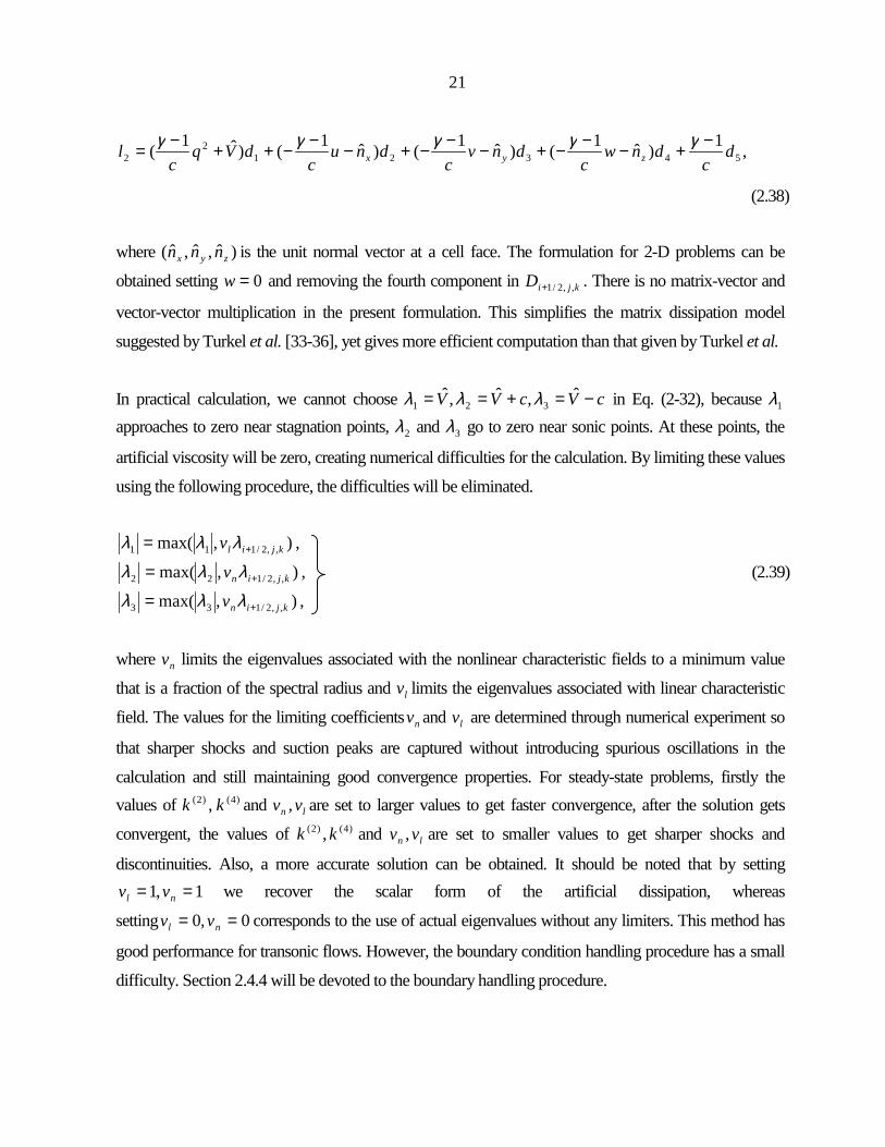
In practical calculation, we cannot choose cVcVV −=+== ˆ,ˆ,ˆ321 λλλ in Eq. (2-32), because 1λ

approaches to zero near stagnation points, 2λ and 3λ go to zero near sonic points. At these points, the

artificial viscosity will be zero, creating numerical difficulties for the calculation. By limiting these values

using the following procedure, the difficulties will be eliminated.

),max( ,,2/111 kjilv += λλλ ,

),max( ,,2/122 kjinv += λλλ , (2.39)

),max( ,,2/133 kjinv += λλλ ,

where nv limits the eigenvalues associated with the nonlinear characteristic fields to a minimum value

that is a fraction of the spectral radius and lv limits the eigenvalues associated with linear characteristic

field. The values for the limiting coefficients nv and lv are determined through numerical experiment so

that sharper shocks and suction peaks are captured without introducing spurious oscillations in the

calculation and still maintaining good convergence properties. For steady-state problems, firstly the values of )4()2( , kk and ln vv , are set to larger values to get faster convergence, after the solution gets

convergent, the values of )4()2( , kk and ln vv , are set to smaller values to get sharper shocks and

discontinuities. Also, a more accurate solution can be obtained. It should be noted that by setting 1,1 == nl vv we recover the scalar form of the artificial dissipation, whereas

setting 0,0 == nl vv corresponds to the use of actual eigenvalues without any limiters. This method has

good performance for transonic flows. However, the boundary condition handling procedure has a small

difficulty. Section 2.4.4 will be devoted to the boundary handling procedure.

22

2.4.3 Matrix Dissipation Model (MDM (2)) with Second-order Difference and Linear or Parabolic Interpolation for Primitive Variables MDM (2) is very similar to MDM (1). The numerical flux at cell face is constructed by the following way:

)()())(ˆ)(ˆ(21ˆ

,,2/11

,,2/1LR

kjidRL

kji QQRREQFQFF −Λ−+= +−

+ , (2.40)

where dE is the dissipation coefficient, the standard value is 0.5, but it can be adjustable. The definitions

of 1,, −Λ RR are the same as MDM (1), but the values of primitive variables ),,,,( pwvuρ at cell faces are

obtained using linear or parabolic interpolation of the values at cell centers because the cell-centered finite

volume scheme is used in the present study. This method is more convenient to handle the boundary

conditions than MDM (1), because we can use the same order interpolation as inner points for boundary

points by using the inner points on one side of the corresponding boundary. So the calculation at

boundary points is consistent with the calculation of the inner points, resulting in the over all good

performance for the whole domain. In addition to this advantage, this method can obtain higher accuracy

by using parabola or higher order interpolations for primitive variables. Furthermore, in a practical

calculation, a limiter must be used to prevent numerical oscillation. In the present study, the following

limiter is chosen:

εε

+∇∆+∇−∆+∇∆4)(3

42 , 11 , −+ −=∇−=∆ iiii ffff , (2.41)

where ε is a very small positive parameter to use to avoid a zero denominator in smooth region, f is a any

primitive variable, i is the index of a grid cell in one of the coordinates.

23

2.4.4 Boundary Conditions for MDM (1)

This section is devoted to the boundary handling procedure for MDM (1). Near the far-field and

downstream boundaries, information on the flow variables at the “ghost” cells that surround these

boundaries is used to construct the dissipation term. Near the solid boundaries, the linearly distributed

flow variables are implied in forming the derivatives needed for the dissipation term, which results in zero dissipative flux at the solid boundaries at 2/3=j . The grid stencil near the solid wall is presented in

Figure 2.1. In our dissipation model, the fourth-difference is included. The standard five-point difference

stencil must be replaced at the first two interior mesh cells.

Let jd denote the actual dissipation for a mesh cell 3,2=j in the direction represented by index j and

assume 0.1)4()4()2()2( == ελελ , we have

.

,

),()(

,

34)2(2/7

23)2(2/5

)4(2/5

)4(2/7

)2(2/5

)2(2/72/52/73

)4(2/5

)2(2/52/52/32/52

QQDQQD

DDDDDDDDDDDDD

−=

−=

−+−=−=

+==−=

(2.42)

The second-order dissipation term is calculated straightforward, by setting 2/3D equal zero. This implies

that the dissipation terms do not impair the no-flux boundary condition imposed at 2/3=j . When the

solution at cell 2=j is processed, the dissipation at interface 2/5=j is only considered.

.2

,2

2/52/72/9)4(2/7

2/32/52/7)4(2/5

QQQDQQQD

∆−∆+∆−=

∆−∆+∆−= (2.43)

The calculation for 2/7D is straightforward, whereas the calculation for )4(

2/5D has a little trouble because 2/3Q∆ is unknown, but from linearly distributed variables we have

2/52/3 QQ ∆=∆ . (2.44)

Now we have

24

2/52/7)4(2/5 QQD ∆+∆−= . (2.45)

From the discussion above, no “ghost” point at the solid boundary is needed, so the “ghost” point 1=j

can be removed from our calculated domain.

J=9/2

J=7/2

J =5/2

J=3/2 solid wall

Figure 2.1: The

J=2

J=4

J=1

g

J=3

J=1/2

rid stencil near the solid wall.

25

The physical boundary condition at the solid wall is enforced by no penetration condition with

0ˆˆˆˆ =++= wnvnunV zyx . (2.46)

The only contribution to the numerical flux at the solid wall is the pressure p, so the numerical flux at the

solid wall can be written as follows:

=

+

+

+

=

∫∫∫

∫∫∫∫

∫

0ˆ

ˆ

ˆ0

ˆ]ˆˆ[

]ˆˆ[

]ˆˆ[

ˆ

ˆ

0

2/3

σσσ

σρσρσρσρ

σρ

pdnpdnpdn

dVhdpnVwdpnVvdpnVu

dV

F

z

y

x

z

y

x

. (2.47)

2.5 Matrix Compressible Vorticity Confinement Model (MCVC)

According to Turkel et al. [33-36], the matrix dissipation model works better than the scalar dissipation

model. There is a counterpart of matrix dissipation model for CVC, which is called Matrix Compressible

Vorticity Confinement (MCVC). Matrix confinement scales the scalar confinement according to the

egenvalues of the flux Jacobians QG

QF

∂∂

∂∂ ˆ

,ˆ

and QH∂∂ ˆ

. We take

zyx SSSS ˆˆˆ ++= (2.48)

with

26

×−

×−=

iunE

inEAS

cc

cc

x

ˆ).(00

ˆ).ˆ(0

ˆˆ

'

'

ωρ

ωρ

D

, (2-49)

and

×−

×−=

jvnE

jnEBS

cc

ccy

ˆ).(0

ˆ).ˆ(00

ˆˆ

'

'

ωρ

ωρ

v

, (2.50)

×−×−

=

kwnEknE

CS

cc

cc

z

ˆ).(

ˆ).ˆ(000

ˆˆ

'

'

ωρωρD

, (2.51)

where QGB

QFA

∂∂≡

∂∂≡

ˆˆ,ˆˆ and

QHC∂∂≡

ˆˆ , cn is defined in Eq. ( 2.4) and ω is defined in Eq. ( 2.5), and

'cE is the confinement parameter for MCVC. The detailed formulation of matrix-vector multiplication is

defined in Eqs. (2.33-2.39). However, they are evaluated at the cell center instead of at cell faces because

S is the source term, and the eigenvalues are replaced by

wnvnunU

nnncUnnncUU

zyx

zyxzyx

++=

++−=+++== 2223

22221

~,~,~ λλλ, (2.52)

where ),,( yyx nnn is the averaged of the normal vectors at the two cell faces across a same coordinate .

Therefore, matrix confinement implicitly contains the grid size as a scaling factor. This is because

numerical discretization errors are related to the grid size and the confinement is constructed to try to

27

cancel the numerical disretization errors in vortical regions. Therefore, the confinement term should be

related to the grid size, and the grid size is a reasonable scaling factor.

2.6 The Choice of the Values of the Free Parameters In the present study, the dissipation parameters )4()2( , kk and dE , and the confinement parameter cE or

'cE all are free parameters, which are chosen by the researcher. Generally speaking, the values of )2(k

and )4(k are in the range of 0.01-0.5, and the typical value for dE is in the range of 0.1-0.6. They are

chosen in such a way the numerical solution is stable. In my opinion, standard values do not exist for all

problems; the researcher should try different values for the same problem and choose the smallest one

which achieves stability. In addition, the value of the confinement parameter must be chosen by the

experience of the researcher and it depends on the problem solved. By my experience, generally speaking,

the value of the scalar confinement parameter cE ranges from )1000

1(O to )101(O . When matrix

confinement is used, the parameter 'cE is larger than the equivalent value of the scalar confinement

parameter because the matrix confinement implicitly contains the grid size as a scaling factor.

If the problem solved has analytical solution, or other computational results, or the experimental results

available, then the value of the confinement parameter may be tuned by comparison with these results.

Otherwise, the value of the confinement parameter may be tuned based on experience with similar flow

problems. In extreme cases, when very large values of confinement parameter are used, the solution with

confinement may appear to become chaotic. In other cases, too large a value of confinement will produce

non-physical flows. In some instances, flows which would be expected to separate, will not with very

large values of confinement are used. More details bout this will be discussed in Chapter 3 - Chapter 7.

28

Chapter 3 Vortical Solutions of the Conical Euler Equations

In this chapter we will first discuss the previous studies for conical flows over the last two decades, then

describe the detailed formulations for Conical Euler Equations (CEE) and the special procedures of

Compressible Vorticity Confinement (CVC) for conical flows; secondly, we will present the details about

grid generation, finite-volume formulation and boundary handling procedures; and finally we will give

some of our computational results and analysis for conical flows past flat delta wings.

3.1 Introduction

Leading-edge vortex flows in particular are of great interest in modern CFD because leeward vortices are

very important for lift and stability of flight. We take them as our application because a flat plate delta

wing of very simple geometry in high speed and high angle of attack flight can produce a rich variety of

shock/vortex interaction patterns. In the general situation, flow separates at the leading edge of the wing,

resulting in large primary vortices on the leeward of the wing with smaller viscous-induced secondary

vortices beneath them. Most of the researchers model the vortex using a set of governing equations:

potential equation, Euler equations and NS equations. Here we only consider the Euler equations in the

remainder of this chapter.

29

The numerical method consists of discretizing the Euler equations on a grid and solving the resulting set

of algebraic equations numerically. The Euler equations are more attractive as a solution for conical

vortex flows, because they admit distributed vorticity as a solution and cost less than NS equations. They

can model the primary vortex and shock wave with the secondary separation or viscous effects ignored.

Solutions of Euler equations with central-difference conservation schemes have been carried out by

Powell [11], Rizzi [37], Rizzi and Eriksson [38], Murman et al. [39], Newsome [40], Kandil and Chuang

[41] and others. Upwind-difference conservation schemes have been used by Newsome and Thomas [42],

Chakravarthy and Ota [43]. A characteristic-based non-conservative scheme has been used by Marconi

[44]. Grossman used the transonic numerical techniques to solve the conical flow equation and made

remarkable progress in developing this methodology [45]. All of these references gave reasonable

estimates for the pressure coefficient on the wing. However, some of them over-predicted the suction

peak and predicted more outboard position of the primary vortex than the experiments.

Hu and Grossman used the CVC method to calculate the flows over flat delta wings [46] and eliminated

the over-prediction of the suction peak of the pressure coefficient due to the primary vortex, obtaining

good agreement with experimental results. This may be explained by the fact by using vorticity

confinement the location of the primary vortex is closer to the experiments and the velocity distribution

near the primary vortex matches better to actual flow pattern than the other calculations. As a result, the

Mach numbers of the flows on both side of the cross flow shocks located near the wall of the flat plate

and the primary vortex are more closer to the measured values, as well as the positions of the primary

vortex and the cross flow shocks. Furthermore, in this complex supersonic vortex dominated flow, the

pressure coefficient not only depends on the primary vortex, but also depends on the cross-flow shocks

and their interaction. Vorticity confinement appears to play an important role in obtaining good

agreement with the experiments.

The purpose for this calculation was to test how the CVC method works with complex supersonic vortex

dominated flows. In this calculation, the CVC method reduced the diffusion of the vorticity of the

primary vortex, compared to the traditional methods.

30

3.2 Governing Equations

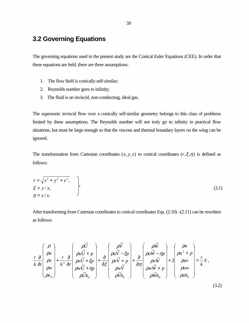
The governing equations used in the present study are the Conical Euler Equations (CEE). In order that

these equations are held, there are three assumptions:

1. The flow field is conically self-similar;

2. Reynolds number goes to infinity;

3. The fluid is an inviscid, non-conducting, ideal gas.

The supersonic inviscid flow over a conically self-similar geometry belongs to this class of problems

limited by these assumptions. The Reynolds number will not truly go to infinity in practical flow

situations, but must be large enough so that the viscous and thermal boundary layers on the wing can be

ignored.

The transformation from Cartesian coordinates ),,( zyx to conical coordinates ),,( ηξr is defined as

follows:

./,/

,222

xzxy

zyxr

==

++=

ηξ (3.1)

After transforming from Cartesian coordinates to conical coordinates Eqs. (2.10) –(2.11) can be rewritten

as follows:

Skr

uhuwuv

puu

hWpWw

WvpWu

W

hVVw

pVvpVu

V

hUpUwpUvpUu

U

rkr

ewvu

tkr

O

=

++

+

−

∂∂+

+−

∂∂+

+++

∂∂+

∂∂

0

2

000

2 2

~~

~~

~

~~

~~

~

~~~~

~

ρρρ

ρρ

ρρρ

ηρρ

η

ρρ

ρξρ

ρ

ξ

ρηρξρ

ρρ

ρρρρρ

,

(3.2)

31

where

.~,~

,~,1 22

uwW

uvV

wvuU

k

ηξ

ηξ

ηξ

−=

−=

++=

++=

(3.3)

The details about how to get Eq. (3.2) are presented in Appendix B. As we know that the boundary

conditions and the vorticity confinement must satisfy the conical assumption 0=∂∂r

. In order to make

the boundary conditions conical, the boundaries of the computational domain must coincide with specify

“rays”; for example, the grid corresponding to bow shock, the wing wall and leading edges of the wing

must be generated by rays emanating from the apex. The class of inviscid supersonic flows with shocks

attached at the wing apex will satisfy these conical boundary conditions. For vorticity confinement term S,

the component in ray direction of “body force” bf

must be zero so that vorticity confinement is

consistent with the conical assumptions. Otherwise, there will be acceleration in the ray direction, and as a

result, rQ∂∂ will not be zero (Q is the state variables). The details of vorticity confinement term S will be

discussed in the next section.

According to conical assumptions, the second term on left side of Eq. (3-2) can be removed. Hence we

have

.2

~~

~~

~

~~

~~

~

0

2

00

Skr

uhuwuv

puu

hWpWw

WvpWu

W

hVVw

pVvpVu

V

ewvu

tkr

O

=

++

+

−

∂∂+

+−

∂∂+

∂∂

ρρρ

ρρ

ρρρ

ηρρ

η

ρρ

ρξρ

ρ

ξ

ρρρρρ

(3.4)

Eq. (3.4) is called CEE.

32

3.3 Vorticity Confinement Procedure

The construction of vorticity confinement for CEE is the essential issue in this chapter. How do we build

the vorticity confinement term S so that it is consistent with the conical assumptions as mentioned in

section 3.2? The component of “body force” bf

in r direction in conical coordinates must be zero.

Otherwise, bf

will give the fluid “particles” acceleration in ray direction. If we take cross-flow vorticity

rω (Appendix B) that is perpendicular to cross-flow plane ηξ − as the vorticity vector in the vorticity confinement procedure, then the unit vector cn defined as

||)(|||)(|ˆ

r

rcn

ωω

∇∇

−= (3.5)

will lie on cross-flow plane ηξ − , hence “body force” bf

defined as

rccb nEf ω

×−= ˆ (3.6)

must lie on cross-flow plane ηξ − also.

After some algebraic manipulation (the details can be found in Appendix B), we found the relationships

between the unit Cartesian coordinate vector )ˆ,ˆ,ˆ( kji and unit conical coordinate vector )ˆ,ˆ,ˆ( ηξ iiir , and

the expression of cross-flow vorticity vector rω as follows:

),ˆ)1(ˆˆ(111ˆ

),ˆˆ)1(ˆ(111ˆ

),ˆˆˆ(1

1ˆ

2

222

2

222

22

kjii

kjii

kjiir

ξξηηηξξ

ξηηξηξη

ηξηξ

η

ξ

++−−+++

=

−++−+++

=

++++

=

(3.7)

33

and

,ˆˆ0rrrr ii

rωωω == (3.8)

where

,0

rrωω = (3.9)

).()(0 ηξξηξηηξ ηξηηξξω vvuwwuvw ++−+++−= (3.10)

From Appendix B we can obtain three conical coordinate coefficients ηξ hhhr ,,

.1

1

,1

1

,1

22

2

22

2

ηξξ

ηξη

η

ξ

+++

=

+++

=

=

rh

rh

hr

(3.11)

Now we can calculate the “body force” bf

as follows:

),ˆ(ˆˆ rrccrccb inEnEf ωω ×−=×−=

(3.12)

where cn is calculated using Eq. (3.5).

For convenience, let us define a scalar variable φ as

rrrr i ωωωφ === ˆ , (3.13)

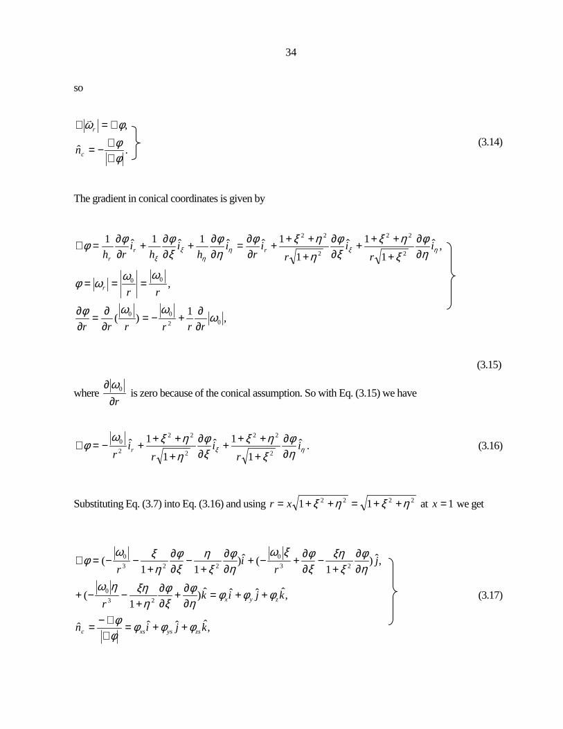
34

so

.ˆ

,

φφφω

∇∇−=

∇=∇

c

r

n

(3.14)

The gradient in conical coordinates is given by

,1)(

,

,ˆ1

1ˆ1

1ˆˆ1ˆ1ˆ1

0200

00

2

22

2

22

ωωωφ

ωωωφ

ηφ

ξηξ

ξφ

ηηξφ

ηφ

ξφφφ ηξη

ηξ

ξ

rrrrrr

rr

ir

ir

ir

ih

ih

irh

r

rrr

∂∂+−=

∂∂=

∂∂

===

∂∂

+

+++∂∂

+

+++∂∂=

∂∂+

∂∂+

∂∂=∇

(3.15)

where r∂

∂ 0ω is zero because of the conical assumption. So with Eq. (3.15) we have

ηξ ηφ

ξηξ

ξφ

ηηξω

φ ir

ir

ir r

ˆ1

1ˆ1

1ˆ2

22

2

22

20

∂∂

+

+++∂∂

+

+++−=∇ . (3.16)

Substituting Eq. (3.7) into Eq. (3.16) and using 2222 11 ηξηξ ++=++= xr at 1=x we get

,ˆˆˆˆ

,ˆˆˆˆ)1

(

,ˆ)1

(ˆ)11

(

230

230

2230

kjin

kjikr

jr

ir

zsysxsc

zyx

φφφφφ

φφφηφ

ξφ

ηξηηω

ηφ

ξξη

ξφξω

ηφ

ξη

ξφ

ηξω

φ

++=∇∇−=

++=∂∂+

∂∂

+−−+

∂∂

+−

∂∂+−+

∂∂

+−

∂∂

+−−=∇

(3.17)

35

where

.

,

,

222

222

222

zyx

zzs

zyx

yys

zyx

xxs

φφφφφ

φφφ

φφ

φφφφφ

++

−=

++

−=

++

−=

(3.18)

Also, rrr i

ωω = is known. So we have

)ˆˆˆ(1

ˆ22

00 kjiir rr ηξ

ηξωωω ++++

== . (3.19)

Now we can build bf

as

,ˆˆˆ

111

ˆˆˆ

ˆ

220

220

220

kfjfifkji

EnEf bzbybxzsysxscrccb ++=

++++++

−=×−=

ηξηω

ηξξω

ηξω

φφφω

(3.20)

with the three components in Cartesian coordinates given by

36

).(1

),(1

),(1

220

220

220

ysxsc

bz

xszsc

by

zsysc

bx

Ef

Ef

Ef

φξφηξ

ω

ηφφηξ

ω

ξφηφηξ

ω

−++

−=

−++

−=

−++

−=

(3.21)

Finally we get the expression of the vorticity confinement term as follows:

−+−+−++

−

−++

−

−++

−

−++

−

=

++

=

)]()()([1

)(1

)(1

)(1

0

)(

0

220

220

220

220

ysxsxszszsysc

ysxsc

xszsc

zsysc

bzbybx

bz

by

bx

wvuE

E

E

E

wfvfuffff

S

φξφηφφξφηφηξ

ρω

φξφηξ

ρω

ηφφηξ

ρω

ξφηφηξ

ρω

ρρρρ

.

(3.22)

The CVC procedure for supersonic conical flows was also described in the paper of Hu and Grossman

[46].

3.4 Solution Procedure

In the present study the scheme used to solve conical equations Eq. (3.4) is a finite-volume, cell-centered,

multi-stage time-stepping Runge-Kutta scheme that is described in Chapter 2. The state variables are

stored at the cell-center. The grid generation, finite volume formulation, flux integration, vorticity

confinement implementation, and boundary conditions will be discussed in this section.

37

3.4.1 Grid Generation

A modified Joukowski transformation is used to generate grid with flat plate geometries. The grid on

cross-flow plane ηξ − is generated from the complex plane ζ . The transformation is given by

ζζηξ ˆ/ˆ 2ai +=+ , (3.23)

where

,2/]tan)2/[tan(

,4/]tan)2/([tan,1

222

δπζ

δπ

+Λ−=

−Λ−=−=

b

ai

D

(3.24)

where Λ is the leading-edge sweep angle of the wing, δ is the half of the vertex angle of the elliptic

cone; and the radius of the circle in complex plane ζ

corresponding to the wing elliptic section in ηξ −

plane is bζ

. The flat plate wing is simply obtained by setting 0=δ . The grid points at ),( kj are

generated by

,sin)(

cos)(

,

2

,,

,,

2

,,

jkj

kjkj

jkj

kjkj

a

a

θζ

ζη

θζ

ζξ

K

K

K

K

−=

+=

(3.25)

where

),1max

121(2

)],1max

1)(1(1ln[,,

,,

−−−=

−−−−

−−= −

jj

kke

j

kokbkbkj

πθ

σζζ

ζζ σ

(3.26)

38

where ko,ζ

is the outer boundary position, (j, k) is the index of grid cell, jmax and kmax are the

maximum indices in ηξ , directions. σ is a grid stretching parameter. σ is 2.0 in the present calculation.

Grid is set to 6464× . This method was originally proposed by Marconi [45], yielding near-conformal

grids with good resolution near the surface of the wing. A sample grid generated by this method is shown

in Figure 3.1

3.4.2 Finite Volume Formulation

The factor κr in conical Euler Eq. (3-4) can be simplified as follows:

xxzyxr =

++

++=

++

++=

22

22

22

222

1

1

1 ηξ

ηξ

ηξκ. (3.27)

Solved at 1=x , Eq. (3-4) can be rewritten as follows:

SFHGtQ =+

∂∂+

∂∂+

∂∂ 2

~~

ηξ, (3.28)

where

+=

+

−=

+−

=

=

0

2

00

,~

~~

~

~,

~~

~~

~

~,

uhuwuv

puu

F

hWpWw

WvpWu

W

H

hVVw

pVvpVu

V

G

ewvu

Q

O ρρρ

ρρ

ρρρ

ηρρ

ρρ

ρξρ

ρ

ρρρρρ

. (3.29)

S is calculated using Eqs. (3.12)-(3.22). The discretization of the CEE (3.28) is formulated over a cell on the cross-flow plane ηξ − . This gives the following:

39

∫ ∫∫ ∫∫ ∫∫ ∫ ΩΩΩΩ=+

∂∂+

∂∂+

∂∂ ηξηξηξ

ηξηξ dSddFdddHGdd

tQ 2)

~~( . (3.30)

Using Gauss's divergence theorem, Eq. (3-30) can be rewritten as follows:

SAFAdHdGt

QA ccc =+−+∂∂

∫ Ω∂2)( ξη , (3.31)

Figure3.1: The sample grid for a flat plate delta wing.

40

where cA is the area of the cell, the overbar denotes an average value over the cell. Solving t

Q∂∂ , the

time average rate of change of the state vector Q within a cell, gives the following:

)2()(1 SFdHdGAt

Qc

−−−−=∂∂

∫ Ω∂ξη . (3.32)

The flux integration )( ξη dHdG −∫ Ω∂is calculated by a trapezoidal integration around the cell. This

gives the following:

)])((21))((

21[)( 12211221 ξξηηξη −+−−+=− ∑∫ Ω∂

HHGGdHdGfaces

. (3.33)

where the subscripts for G and H denote the two cells that define the face, the subscripts for ξ and η

denote the two end points of the grid cell face (see Figure 3.2) , ordered so that the integral is carried out

in a counter-clockwise direction. This is usually second-order accurate, regardless of the stretching of the

grid [33]. The cell-average of the source term is calculated by the cell average variables, because our

scheme is cell-centered scheme, so the calculation of SF , is straightforward.

The cell area cA is calculated by the following formula according the grid stencil shown in Figure 3.2.

)])(())([(21

42134213 ηηξξξξηη −−−−−=cA . (3.34)

The artificial matrix dissipation model MDM (1) described in Chapter 2 and a 3-stage Runge-Kutta time

integration scheme is used.

To enhance the convergence to steady-state solution, local time-stepping is used. The time-step is

calculated by

41

∫ Ω∂+

=∆dlcV

ACFLt c

)ˆ(. , (3.35)

where c is the local speed of sound, and V is evaluated at cell face that is calculated by averaging the values of the two cells that define that face.

3.4.3 Boundary Conditions

There are 4 boundary conditions that must satisfy with the Euler equations:

1. No penetration condition enforced at the solid wall that has been discussed in Chapter 2;

2. Free-stream conditions upstream of the bow shock;

3. The Kutta conditions at the leading-edges;

1. The symmetry condition at the symmetry plane.

The free-stream condition is implemented numerically by placing the outer boundary of the com-

putational plane outside the bow shock and setting the state vector at each point on the outer boundary η 4 3

(i , j) 1 2 ξ

Figure 3.2: The grid stencil on a cross-flow plane.

42

to the free stream state vector. The outer boundary chosen is an expanded Mach cone, shifted to lee-side

to account for the angle of attack. This gives the following:

,coscos

,sin2 φφη

φξ

ss

s

zrr

+=

= (3.36)

where

),10sin3,sin3max(

),1(sin3

0

1

α=

=∞

−

s

s

zM

r (3.37)

where φ is the angle between the ray in the domain and the ray at boundary. The Kutta condition

physically implies that the cross-flow leaves the leading edge smoothly. This rules out the possibility of

infinite velocity at the leading edge. In the real flows, the viscosity sets the Kutta condition. Similarly, in

numerical simulation the artificial viscosity in the region of leading edge enforces the Kutta condition. In

the present calculation, the coefficients of second-order dissipation term for MDM (1) at several cells in

the vicinity of the leading edge are set to the maximum value in the whole domain to enforce the Kutta

condition.

The symmetry plane is introduced so that the flow past a wing at zero yaw angle can be solved on a half

plane. The condition to be enforced at the symmetry plane is that the velocity component v, through

symmetry plane, is zero. In the present study this was implemented by initially setting v to zero and

zeroing out the distributed flux in the y-direction in the continuing calculation.

3.5 Numerical Results for the Conical Euler Equations

In this section we will present the numerical results for CEE using the numerical method MDM (1) along

with the MCVC method described in Chapter 2 and the procedures described in sections 3.1- 3.4.

Representative plots of some flow variables will be presented and discussed. A part of the results that will

43

be presented here was also discussed by Hu and Grossman in Ref. [46]. Two cases will be used to

illustrate the capability of CVC procedure in the calculations of complex supersonic vortex dominated

flows. One case is the calculation for the flow over a flat delta wing with a moderate supersonic Mach

number and an angle of attack )75,12,7.1( 00 =Λ==∞ αM and the other case is with a higher Mach

number and angle of attack )75,20,8.2( 00 =Λ==∞ αM . The calculations for these two cases were performed on the 6464× stretched grid on the cross-flow plane ηξ − (see Figure 3.1) with dissipation

parameters set to 005.0,1.0 )4()2( == kk and the confinement parameter 0.15' =cE . Note here that we

are using matrix confinement which effectively scales the confinement parameter by the grid size.

Elsewhere in this dissertation, scalar confinement is used with correspondingly small values of the confinement parameter )1.0001.0:( −cE . Several set of values of dissipation parameters were tested at

the beginning of the calculations so that the added artificial dissipation term was small as much as

possible. When the values of the dissipation parameters were too small, the numerical solution showed

oscillation. The current ones were the right ones that were found so that the numerical solutions were

stable. It was time-consuming to choose the value of the confinement parameter in these cases. First,

several small values were tested. By the observation of the scope of the vortex we saw that the vorticity

was still be diffused from the center of the vortex. Under these circumstances the computed vortex region

was larger than the measured one in the experiment. Next, several larger values of confinement

parameters were tested, until the size of the primary vortex closed to the experimental one. The current

one was the right one used in the present calculation to prevent the vorticity from diffusing away by the

numerical dissipation and keep the right size of the primary vortex.

All of the plots in this section are on the cross-flow plane ηξ − . The coordinate axes are scaled by local

half span of the wing and denoted by b/ξ and b/η respectively. The wing is at 0/ =bη and extends

from 1/ −=bξ to 1/ =bξ . Because the flow is with zero yaw angle flight, the flow is symmetry

about 0/ =bξ , so only positive ξ plane is shown. The contour plots only show the qualitative

information such as shock, vortex, and vortex/shock interactions, while the pressure coefficient profile on

the surface of the wing and the comparison with experimental and other computational results will give

the quantitative information.

In order to evaluate the accuracy of the basic code, we performed a calculation of a 015 half-angle circular cone at zero angle of attack. The computation is done without confinement. The dissipation

parameters in MDM (1) )2(k was set to 0.5, and )4(k was set to 0.01. The calculation was performed on a

44

grid with 64 mesh points in circumferential direction (half cone) and 51 mesh points in the azimuthally

direction. The pressure coefficient distribution in the shock layer is presented in Figure 3.3. The

agreement with the accurate Taylor-Maccoll analytical solution [47] is excellent. The bow shock is

accurately captured within two mesh points.

3.5.1 Topology of the Conical Flows

The topological information about the conical flow is presented through cross-flow velocity vector plots

and cross-flow streamline plots. Both the velocity vector and streamline plots are based on the cross-flow velocity uvv ξ−=~ and uww η−=~ . The cross-flow velocity vector plots are generated by drawing at

each cell center, an arrow whose vector component are proportional to the local values of v~ and w~ .

3.5.1.1 Case 1 --- 00 75,12,7.1 =Λ==∞ αM

Figure 3.4 presents the velocity vectors. The primary vortex and the feeding sheet are clearly seen in this

Figure. The cross-flow streamlines are presented in Figure 3.5 that shows the primary vortex, the node at

the windward symmetry point, and saddle points at the leeward symmetry point and on the windward

side of the wing near the leading edge. The underside of the vortex shows a reverse curvature that is the

evidence of a cross-flow shock underneath the primary vortex. Figure 3.5 shows the good qualitative

agreement between the present calculation and the experiment, including the shape and position of the

primary vortex and the leading edge vortex sheet.

3.5.1.2 Case 2 --- 00 75,20,8.2 =Λ==∞ αM Figure 3.6 presents the cross-flow velocity vectors. The feeding sheet and primary vortex is shown clearly,

as well as three cross-flow shocks: a shock above the vortex, where the flow direction is inboard, a shock

inboard of the vortex, where the flow direction is towards the wing, and a shock under the vortex, where

the flow is outboard, this reverse cross-flow shock is under the vortex. The shocks above and inboard of

the vortex are representative of high angle of attack cases. Figure 3.6 also shows the blowups of the

vortex core, the feeding sheet and the reverse cross-flow shock. The feeding sheet shows a large change

in the magnitude of the cross-flow velocity across a very small region, with the vector remaining parallel

45

through the sheet. The cross-flow shock is characterized by a change in both magnitude and the direction

of the vectors. The cross-flow streamlines are presented in Figure 3.7 that shows a node at the windward

symmetry point and saddle points at the leeward symmetry point, the leading edge and the outboard

portion of the windward side of the wing. The vortex has a high degree of reverse curvature, suggesting a

strong cross-flow shock underneath the vortex. The comparison with the experiment in Figure 3.7 shows

that a good qualitative agreement was obtained in the present calculation, including the shape and the

position of the primary vortex and the leading edge vortex sheet.

Figure 3.3: Pressure distributions in the shock layer of a circular cone with 150 half angle at zero angle of attack and 0.2=∞M . 3.5.2 Pressure Coefficient Profile

The variable considered here is the static pressure coefficient distributed on the surface of the wing.

46

2

2 ∞∞

∞−=

Mp

ppc p γ . (3.38)

Figure 3.8 presents the pressure coefficient profile on a flat delta wing with 00 75,12,7.1 =Λ==∞ αM and Figure 3.9 shows the pressure coefficient profile on a flat delta wing

with 00 75,20,8.2 =Λ==∞ αM . In the same figure we presented the results calculated both with

confinement and without confinement, experiment data of Miller and Wood [2] as discussed in Ref. [11],

and the solution of Euler equations of Powell [11] performed on an equivalent 128128× grid with local

grid refinement in the vicinity of the vortex and the leading edge. From Figure 3.8 we see that even

though the solution with vorticity confinement was not completed with locally refined grid and was

performed with a quarter number of grid points of that used by Powell, the agreement with the

experiment data appear to be better in the inboard and the core region of the vortex; the over-prediction

suction peak under the primary vortex was eliminated. The reason has been discussed previously in the

introduction of this chapter. We note that our solution without confinement shows a reduced suction peak.

However, this solution shows larger size of the primary vortex than the measured one in the experiment

because it was diffused by the numerical dissipation inherently related to the numerical discretization.

Figure 3.9 shows that the leeward pressure is nearly constant for the flight at a higher angle of attack and

higher Mach number, the present computed solution agrees well with the measured data and the

computational result of Powell. Figure 3.10 presents the contours of the cross-flow Mach numbers for the

case with 00 75,12,7.1 =Λ==∞ αM . Figure 3.11 shows the contours of the cross-flow Mach

numbers for the case with 00 75,20,8.2 =Λ==∞ αM . From the theoretical analysis we can conclude

that the Mach number is nearly constant on the windward side, increasing through the expansion at the

leading edge, reaching to its maximum values above and below the vortex. The deceleration occurs

through the cross-flow shock. The gradients are highest at the cross-flow shock, the sheet, and the core

region where the cross-flow Mach number reaches zero. The pressure coefficient contours for the two

cases are presented in Figure 3.13 and Figure 3.14. The pressure coefficient reaches the minimum in the

core of the vortex. It is nearly constant on the windward and on the leeward side inboard of the vortex.

The expansion fan is located at the leading edge and the expansion and recompression occurs under the

vortex. Comparing these two figures we can conclude that the case with higher Mach number and an

angle of attack shows stronger windward bow shock than the case with lower Mach number and angle of

attack.

47

From the analyses above, we see that CVC works well in the calculations of the complex supersonic

vortex dominated flows over flat delta wings. It appears that the confinement procedure eliminates the

overshoot of the suction peak of the pressure coefficient in the primary vortex computed in Ref. [11]. In

addition, it appears that the CVC method shrinks the over - predicted size of the primary vortex that may

be caused by the numerical dissipation. However, the bow shock does not appear to be strongly affected

by the confinement, because the conical shock has relatively small vorticity gradients. On the other hand,

the cross-flow shock looks to be strongly affected by confinement, especially the position of the cross-

flow shock, because of the strong vorticity that has strong vorticity gradients. Therefore, It should be

noted that CVC works and only works in the vortical regions in which there exists strong vorticity

gradients.

48

Figure 3.4: The cross-flow velocity vector distributions for a flat plate delta wing at 00 75,12,7.1 =Λ==∞ αM .

Figure 3.5: The experimental result and the present computed streamline distributions on the cross-flow

plane for a flat plate delta wing at 00 75,12,7.1 =Λ==∞ αM . Left --- Experimental vapor screen [2].

Right --- the streamline distributions of the present calculation.

49

Figure 3.6: The cross-flow velocity vector distributions on a flat delta wing at

8.2=∞M , 00 75,20 =Λ=α .

Figure 3.7: The experimental result and the present computed streamline distributions on the cross-flow

plane for a flat plate delta wing at 00 75,20,8.2 =Λ==∞ αM . Left --- Experimental vapor screen [2].

Right --- the streamline distributions of the present calculation.

50

b/ξ

Figure 3.8: The pressure coefficient distributions on a flat delta wing at 00 75,12,7.1 =Λ==∞ αM .

b/ξ

Figure 3.9: The pressure coefficient distributions on a flat delta wing at 00 75,20,8.2 =Λ==∞ αM .

51

Figure 3.10: The Mach number contours for a flat delta wing at 00 75,12,7.1 =Λ==∞ αM .

Figure 3.11: The Mach number contours for a flat delta wing at 00 75,20,8.2 =Λ==∞ αM .

52

Figure 3.12: The pressure coefficient contours for a flat delta wing at 00 75,12,7.1 =Λ==∞ αM .

Figure 3.13: The pressure coefficient contours for a flat delta wing at 00 75,20,8.2 =Λ==∞ αM .

53

Chapter 4 Numerical Simulation of Shock-Bubble and Shock-Vortex Interaction In this chapter we will investigate the vortex structures formed by a moving shock over a circular light-

gas inhomogeneity (both a stationary bubble and a circular vortex) in a channel with a finite width. The

pressure gradient from the shock wave interacts with the density gradient at the edge of the

inhomogeneity to form a vortical layer around the perimeter, and the structure rolls up into a complex

vortex structures.

The purpose for which we did these calculations is to see how CVC works with the vortical layer formed

by the interaction between a moving shock wave and a circular light gas inhomogeneity. We will

qualitatively compare the patterns of the vortical layer with the measured ones in the experiment and

quantitatively compare the pressure, the density and vorticity in the centers of the vortices with the

computed results obtained by using other computational techniques.

4.1 Overview for Previous Studies in Shock-Bubble and

Shock-Vortex Interaction

James et al. performed a detailed numerical study for a weak shock wave passing through an isolated

stationary cylindrical gas inhomogeneity [48]. They utilized a novel shock-capturing scheme in

conjunction with a sophisticated mesh refinement algorithm to solve the two-dimensional compressible

Euler equations for a two-component fluid (air-helium or air-refrigerant 22). They numerically

reproduced the intricate mechanisms that were observed in the experiment. Yang et al. simulated the

54

vortex pair formed by shock-bubble interaction by solving two-dimensional Euler equations with a finite-

difference Flux-Corrected-Transport algorithm (FCT) [9]. Using the numerical results they developed a

relatively simple algebraic model that characterizes the dynamics of the vortex pair and that allows

extrapolation of the numerical results to conditions of more interest in real engineering problems.

Utilizing an adaptive unstructured scheme, Povitsky and Ofengeim studied the interaction between a

vortical density inhomogeneity (VDI) (both stationary light gas bubble and a circular vortex) with a shock

and expansion wave [8].

4.2 Present Studies for Shock-Bubble Interaction

To compare to the computational results of Yang et al. [9] and Povitsky and Ofengeim [8], we used the

finite-volume scheme with MDM (2) and the scalar CVC described in Chapter 2 to perform the calculation of the same problem that was calculated by Yang and Povitsky et al. The dissipation parameter dE was

set to 0.3. The confinement parameter cE was set to 0.005. In the process of calculation, several values of

the dissipation parameter dE were tested, and the smallest one was used so that no oscillation occurred in

the calculation. After the dissipation parameter was chosen, we fixed the value of dE and tuned the value

of the confinement parameter cE . We chose the value of E c in such a way so that we kept the edge of the

vortical layer sharp as much as possible. The computation was performed with a 200600× Cartesian

grid. The initial conditions for the calculation were chosen to match the conditions present in the

experiment of Jacobs [10] who studied the flow formed by a plane shock wave impinged on a laminar jet

of helium injected into air at ambient pressure. The Mach number of the moving shock is 1.1. The density

ratio of light/heavy gas is 0.138.

Figure 4.1 presents the density contours and comparison with the experimental PLIF images [10] that

give the cross-section view of the evolving helium inhomogeneity. The density contours conveyed the

information about organization and stabilization of the vorticity into a stable core. It also provided us the

information about the straining of the vortex pairs and the motion of the light/heavy gas interface. In the time interval st µ373123−= the fluid that did not become part of the vortex core is pinched off as a pair

of upstream tails. At the downstream end, a well-defined thin filament connected the two cores. This

filament stretched and thinned in the vertical direction due to a strong straining motion from the high vorticity cores. In the time interval st µ573373−= , the vortex gradually stabilized and the circulation of

55

the vortex core was obviously noted. In the time interval st µ773573−= , the core induced in each

other a strong, horizontal velocity, thus moving downstream more rapidly than the tails, which stretched

upstream as they trailed behind the core. These tails also experienced strong induced velocities that

caused them to rotate towards the centerline. Figure 4.2 presents the comparison of the present results

and the computed results of Yang et al. [9] using FCT scheme. The present results show much less

numerical diffusion and better agreement with the experiment results. Figure 4.3 shows the comparison

of present results and the results of Povitsky and Ofengeim [8] using an adaptive unstructured scheme; a

good agreement was obtained.

56

Figure 4.1: The comparisons of density contours at (a) st µ123= , (b) st µ373= , (c) st µ573= ,

(d) st µ773= . Left side --- CVC. Right side --- Experiment [10].

57

Figure 4.2: The comparisons of density contours at (a) st µ123= , (b) st µ373= , (c) st µ573= ,

(d) st µ773= . Left side --- CVC. Right side --- FCT [9].

58

Figure 4.3: The comparisons of density contours at (a) st µ123= , (b) st µ373= , (c) st µ573= ,

(d) st µ773= . Left side --- CVC. Right side --- Adaptive Unstructured Algorithm [8].

59

4.3 Present Study for Shock-Vortex Interaction

Povitsky and Ofengeim [8] computed the problems of a moving shock over a circular vortex shown in

Figure 4.4. The initial conditions for the vortex model used their study and in the present study can be

written as follows:

,,/

,/)(

0

≤<+≤

=RrRrBAr

RrRrUru

c

cccθ (4.1)

where

220 c

cc

RRRU

A−

−= ,

(4.2)

220

20

c

cc

RRRRUB

−= .

The parameters used in the present study are listed bellow:

cRR 20 = ,

2.0/ =hl ρρ , (4.3)

5.1=sM .

The maximum tangential velocity cU of the circular vortex is 0.5 times the velocity behind the moving

shock wave. This is one of the cases calculated by Povitsky and Ofengeim [8]. The computational domain is 00 2040 RR × . The large height was used to try to minimize the channel effect.

First we performed the calculation with a fine grid 200600× . Two runs were carried out. One was

completed without vorticity confinement; the other was completed with vorticity confinement. The basic

solver was the finite-volume scheme with MDM (2) with the scalar confinement procedure described in Chapter 2. The dissipation parameter dE was set to 0.3. The confinement parameter E c was set to 0.005.

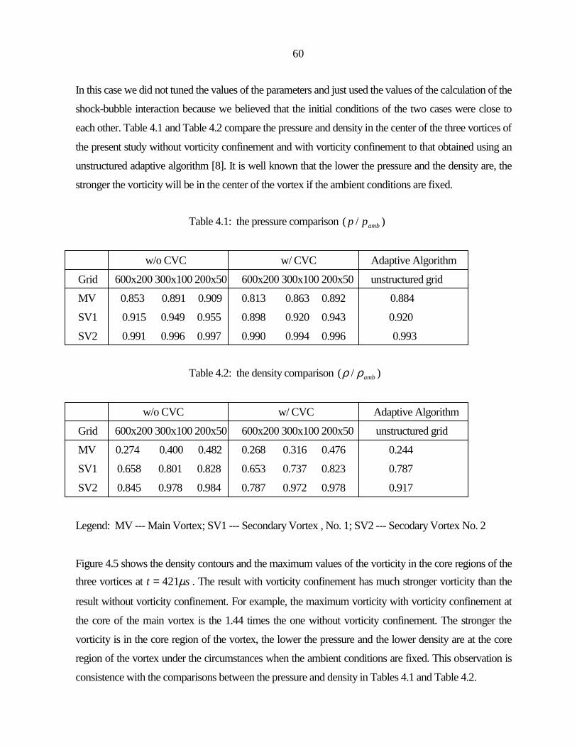
60

In this case we did not tuned the values of the parameters and just used the values of the calculation of the

shock-bubble interaction because we believed that the initial conditions of the two cases were close to

each other. Table 4.1 and Table 4.2 compare the pressure and density in the center of the three vortices of

the present study without vorticity confinement and with vorticity confinement to that obtained using an

unstructured adaptive algorithm [8]. It is well known that the lower the pressure and the density are, the

stronger the vorticity will be in the center of the vortex if the ambient conditions are fixed.

Table 4.1: the pressure comparison )/( ambpp

w/o CVC w/ CVC Adaptive Algorithm

Grid 600x200 300x100 200x50 600x200 300x100 200x50 unstructured grid

MV 0.853 0.891 0.909 0.813 0.863 0.892 0.884

SV1 0.915 0.949 0.955 0.898 0.920 0.943 0.920

SV2 0.991 0.996 0.997 0.990 0.994 0.996 0.993

Table 4.2: the density comparison )/( ambρρ

w/o CVC w/ CVC Adaptive Algorithm

Grid 600x200 300x100 200x50 600x200 300x100 200x50 unstructured grid

MV 0.274 0.400 0.482 0.268 0.316 0.476 0.244

SV1 0.658 0.801 0.828 0.653 0.737 0.823 0.787

SV2 0.845 0.978 0.984 0.787 0.972 0.978 0.917

Legend: MV --- Main Vortex; SV1 --- Secondary Vortex , No. 1; SV2 --- Secodary Vortex No. 2

Figure 4.5 shows the density contours and the maximum values of the vorticity in the core regions of the three vortices at st µ421= . The result with vorticity confinement has much stronger vorticity than the

result without vorticity confinement. For example, the maximum vorticity with vorticity confinement at

the core of the main vortex is the 1.44 times the one without vorticity confinement. The stronger the

vorticity is in the core region of the vortex, the lower the pressure and the lower density are at the core

region of the vortex under the circumstances when the ambient conditions are fixed. This observation is

consistence with the comparisons between the pressure and density in Tables 4.1 and Table 4.2.

61

cU

sM cR

Figure 4.4: A moving shock over a circular vortex model.

Figure.4.5: The density contours at 421 sµ .

0R

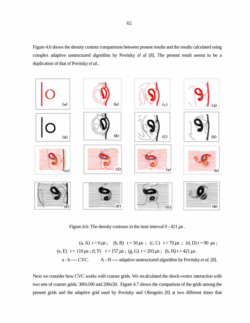
62

Figure 4.6 shows the density contour comparisons between present results and the results calculated using

complex adaptive unstructured algorithm by Povitsky el al [8]. The present result seems to be a

duplication of that of Povitsky et al..

Figure.4.6: The density contours in the time interval 0 - 421 sµ .

(a, A) t = 0 sµ ; (b, B) t = 50 sµ ; (c, C) t = 70 sµ ; (d, D) t = 90 sµ ;

(e, E) t = 110 sµ ; (f, F) t = 157 sµ ; (g, G) t = 203 sµ ; (h, H) t = 421 sµ .

a - h ---- CVC. A - H ---- adaptive unstructured algorithm by Povitsky et al. [8].

Next we consider how CVC works with coarser grids. We recalculated the shock-vortex interaction with

two sets of coarser grids: 300x100 and 200x50. Figure 4.7 shows the comparison of the grids among the

present grids and the adaptive grid used by Povitsky and Ofengeim [8] at two different times that

63

correspond to the time before shock-vortex interaction and the time after shock-vortex interaction. From

the figure we see that the adaptive grid in the core region of the vortex and the region near the shock is

much denser than the present grids, though the present grids in other regions are denser than the adaptive

grid. Figure 4.8 presents the comparison of the density contours between the present results and the

results obtained using an adaptive algorithm [8]. From this figure we see that the agreement is very good,

though the result of the coarsest grid of the present study shows a little dissipation in the core region of the

vortex and the region near the shock, but the solution captured the main vortex features such as the vortex

roll up and pinch off. The result of the finest grid of the present study captured more details of the

complicated vortex structure than the unstructured adaptive algorithm, although the grid in the core region

of the vortex of the present study is coarser than the unstructured adaptive grid. In addition, the

quantitatively comparisons of the pressure and the density in the center of the three vortices are presented

in Table 4.1 and Table 4.2. From these tables we see that CVC works well with coarse grids.

4.4 Conclusion

Many modern CFD schemes, such as the FCT scheme used in present examples are high order finite-

difference schemes which increase CPU loads. These schemes often contain mesh refinement algorithms

and the adaptive unstructured grid algorithms which have complicated logic and are difficult to

implement. Furthermore, an unstructured adaptive algorithm is CPU intensive, because many more grid

points are embedded in the vicinity of the regions with steep gradients such as the vortex core and

discontinuities. Also, if the problem solved is an unsteady problem, the time step is restrictive by the small

adaptive grid cells and the computational grid needs to be reconstructed at beginning of each time step. In

addition, grid adaptation is difficult to implement for complex flows in three dimensions. Compared with

these methods, for vortex dominant flows, CVC is a robust numerical method which requires much less

computation to achieve accurate results.

On the other hand, the CVC method has some drawbacks. In the calculation we observed that when very large values of the confinement parameter were used, such as 4.0=cE in the shock-vortex interaction

problem, the structure of the vortical layer was broken down to many tiny vortices and the confinement

procedure was not effective. The results under this circumstance are presented in Figure 4.9 and appear to

be somewhat chaotic. Furthermore, from the point view of how CVC is constructed, the vorticity

confinement works only in the vortical regions in which there exist strong vorticity gradients. For

64

example, in the calculations of shock-bubble and shock-vortex interaction, before and after interaction,

near the region close to the shock wave, the vorticity gradient is small or equals to zero and the CVC

method has little or no effect. Furthermore, from Figure 4.8 we see that when the grid size increases, the

shock was diffused by the numerical dissipation. Therefore, the dissipation in shock region was not

strongly affected by the confinement, because the CVC term in this region is very small or equals to zero.

However, in the core region of the vortices, the edges of the vortices are still sharp when the grid size

increases, because there exist strong vorticity and strong vorticity gradients and that the CVC term tends

to balance the numerical dissipation.

65

Figure 4.7: The comparison of the grids. (a), (e) the grid layout before and after interaction , unstructured

adaptive grid [8]; (b), (f) the grid layout before and after interaction of the present study, 200x50; (c), (g)

the grid layout before and after interaction of the present study , 300x100; (d), (h) the grid layout before

and after interaction of the present study, 600x20.

66

Figure 4.8: The comparison of density contours at time 157 sµ on different grids. (a) unstructured

adaptive grid [8]; (b) regular Cartesian grid of the present study 600x200; (c) regular Cartesian grid of the

present study 300x100; (d) regular Cartesian grid of the present study 200x50.

67

Figure 4.9: The density contours at (a) t = 90 sµ and (b) t = 157 sµ for the grid 200x50 and cE = 0.4.

68

Chapter 5 Calculations of Flows past Bluff Bodies The study of the flows around bluff bodies is fundamental to the understanding of the mechanisms of

complex 2D and 3D vortex-dominant flows. In this chapter the flows past a 2D square cylinder and a 3D

cube mounted on the floor of a plate channel will be investigated; the qualitative and quantitative

comparisons among Compressible Vorticity Confinement (CVC), Large Eddy Simulation (LES) and

calculation of Reynolds-Average-Navier-Stokes (RANS) equations will be given, and finally some

conclusions will be stated.

The purpose of these calculations is to test how CVC works with complex turbulent flows with massive

separation past bluff bodies. We did these calculations to see how the value of the confinement

parameter impacts the vortex shedding for the flow past a 2D square cylinder and what is the effects of

CVC on the flow patterns of the massive separation of the flow past a surface-mounted cube. At the

same time, we tested the drawbacks of the CVC method in the process of the calculations for these kinds

of flows.

5.1 Introduction

The flows past a 2D square cylinder and a 3D cube produce many complex phenomena such as multiple

separation, reattachment, unsteady vortex shedding, large-scale turbulent structures as well as bimodal

behavior even for relatively simple geometries. Flows past bluff bodies are involved in many realistic

engineering problems. Generally speaking, it is difficult to numerically simulate such flows because they

are the most challenging problems in current CFD. The detailed experimental data for the flows around a

2D square cylinder and a 3D surface-mounted cube are available from Durao [3], Lyn et al. [49,50], and

Larousse, Martinuzzi and Tropea [4,5]. Both cases are test cases that were computed by LES and RANS

69

calculations with various turbulence models and submitted to an LES workshop in 1996, so we can

qualitatively and quantitatively compare the results calculated by CVC with that measured in experiments

and the results calculated by using LES and RANS with various turbulence models.

In practical problems, the Reynolds numbers are very high. The values of viscous terms in Navier-Stokes

equations are much smaller than that of the convection terms. We attempted to simulate those kinds of

problems mentioned above using Euler equations. However, the boundary layer near the wall cannot be

ignored because it is so important in vortex-dominant flows. So no-slip conditions were used in all our

calculations to enforce the viscous flow boundary conditions on the wall. In most Euler calculations, if a

no-slip wall conditions were imposed, an unreasonably thick boundary layer would develop because of

the diffusive nature of the numerical algorithms. However, as we will show in Chapter 7, the CVC

method produces a boundary layer that is a reasonable first approximation to a turbulent boundary layer

in the near wall regions.

In the presents study, the time-dependent Euler equations were solved to get the instanteneous variables ),,,,( pwvuρ . The accuracy for the calculations of complex vortex-dominant flows strongly

depends on the method used, i.e., Franke and Rodi [14], and Bosh [51].

5.2 Calculation of a Flow past a 2D Square Cylinder

In the present study, an explicit fourth-order Runge–Kutta scheme was used for time discretization, and

the finite-volume cell-centered scheme with a second-order matrix dissipation MDM (2) described in

Chapter 2 was used to approximate the convection terms. The dissipation parameter E d was set to 0.3.

The method used to choose the dissipation parameter has been discussed in Chapter 2, Chapter 3 and

Chapter 4. The scalar confinement procedure with different values of confinement parameter E c was

employed. The value of the vorticity confinement parameter was tuned according to the frequency of the

vortex shedding and the velocity profile along the centerline of the square cylinder. The details will be

discussed in the later part of this section. Furthermore, the parabolic approximation [52,53] was used to interpolate the primitive variables ),,,( pvuρ at cell centers to the cell faces where the numerical fluxes

are evaluated.

70

The results for a flow around a 2D square cylinder will be given in this section. The detailed experiment

data is available from Refs. [3,49,50]. There are two similar experiments referenced in the present study.

One was done by Durao et al. [3]. The Reynolds number of this experiment was 14,000; the other

experiment was done by Lyn et al. [49,50]. The Reynolds number of this experiment was 21,400. Rodi

[13] and Murakami [54] reviewed the results of LES and RANS calculations with various turbulence

models for flows past a 2D square cylinder. The calculation domain in the present study consists of 4.5

times the square cylinder dimension upstream, 14.5 times the square cylinder dimension downstream and

5.5 times the square cylinder dimension above and below the cylinder. The present calculation

reproduced the vortex shedding. Figure 5.1 presents the comparisons of CVC, the experiment [49,50],

RANS-RSM [14] and LES-UKAHY2 [13] calculations for streamline distributions at three phases and

pressure, lift coefficient profile vs. non-dimensional time. It should be noted that the time scale of the

present study is not the same as that of the experiment, but the non-dimensional frequency Strouhal

number tS (∞U

fH , f is the shedding frequency, H is the dimension of the square cylinder and ∞U is the

free stream velocity) obtained in the present study is very close to that measured in the experiment

[3,49,50] if the value of the confinement parameter E c was set within prescribed range.

In the present study the free stream Mach number was 0.4; the flow. The non-dimensional vortex

shedding frequency Strouhal number can be calculated as follows:

),/()/())//((

)/())/(()/(/

∞

∞∞∞

∞∞∞∞∞

==

===

tMnaMHatHn

aMHttnaMfHUfHS rt

(5.1)

where t is the non-dimensional time interval, n is the number of vortex shedding in non-dimensional time t, t r is the reference time ∞aH / , ∞M is the free stream mach number. In the calculations, the

compressible Euler equations were solved with free stream Mach number 0.4. In the calculations we

observed that the value of the confinement parameter played an important role to decide the vortex

shedding frequency. No confinement produced the vortex shedding frequency that was smaller by 6 % -

13 % than the measured range in the experiments. As the value of the confinement parameter increased,

the frequency of the vortex shedding increased which was within 1 % - 8 % of the measured range in the

71

experiments. However, when the value of the confinement parameter exceeded a value of =cE 0.005,

the vortex shedding frequency began to decrease, and when the value of the confinement parameter increased further to an extra large value, 5.0=cE , no separation occurred, as a result, no vortex

shedding occurred. The range of the appropriate values of the confinement parameter for this case with

grid 100x90 can be found in Table 5.1. A sample lift coefficient profile is presented in Figure 5.1 from

which we see that n is fallen into the range of 5 - 5.5 in non-dimensional time of 100, and as a result, the

range of the St number equals to 0.135 – 0.138, which is very close to the range measured in the

experiment. From Eq. (5.1) we see that St is only related to the free stream Mach number M∞ and

number of vortices shedding n in non-dimensional time interval t. St does not depend upon the Reynolds

number, which is confirmed experimentally and with LES and RANS calculations. The computed drag

coefficient and lift coefficient are defined as follows:

,

21

,

21

2

2

HV

FC

HV

FC

LL

DD

∞∞

∞∞

=

=

ρ

ρ (5.2)

where DC is the drag coefficient, LC is the lift coefficient, DF is the drag force, LF is the lift force, ∞ρ is

the free stream density, ∞V is the free stream velocity, and H is the dimension of the square cylinder.

In Table 5.1 various integral parameters (e.g. Strouhal number St, drag coefficient CD, etc.) predicted with

various computational methods are summarized with the experimental data. From Table 5.1 we see that

vorticity confinement produced as good agreement with experiment as did the LES and RANS calculations. From the calculations we observed that DC increased as cE increased, because the base

pressure decreases when E c increases. However, The drag coefficient without confinement was predicted smaller by 5 % - 17 % of the measured range of the experiments. In addition, l R decreased when cE

increased, because vorticity confinement prevents the vortices from being diffused; so the length of the

recirculation behind the cylinder will be shorten when E c increases. On the other hand, the length of the recirculation Rl without confinement was predicted larger by 17 % of the measured one in the

experiments. Furthermore, The vortex shedding frequency decreased when the value of the confinement parameter exceeded =cE 0.005. As mentioned above, when an extra large value of the confinement

parameter was used, for example, =cE 0.5, no vortex shedding occurred. In Chapter 7, we will see how

72

the values of the confinement parameter change the velocity profile of the turbulent flow over a 2D flat plate. As a result, we suggest using 02.0001.0 ≤≤ cE for the calculation of the flow past a square

cylinder. Over this range of values, the results are relatively insensitive to the values of cE .

Table 5.1 shows that the LES calculations produced correct DC values in the range of experiments

[49,50]. Some of the LES calculations yielded high and low Strouhal numbers; the reason is not clear. The RANS calculation with RSM produced very low Rl , but the ε−k model with Kato-Launder (KL)

modification ( ε−− kKL ) [51] and the RGN ε−k model [55] yielded correct value of l R compared

with the experiment of Lyn [49,50] and Durao [3]. The ε−− kKL model produced smaller 'DC and

'LC than LES and CVC. However, the RNG ε−k model and TL-RSM calculations [14] produced

similar 'DC and '

LC to LES and CVC.

The time average velocity U along the centerline of the square cylinder is presented in Figure 5.2. The

results of the CVC, LES, RANS and experimental data due to Lyn [49,50] and Durao [3] are included.

From that figure we see that there are large differences in the wake region for the two experimental results

and computed results with different numerical methods. There could be two reasons that cause the large

difference of the recovery behavior behind the square cylinder between the two experiments. One reason

could be the different Reynolds numbers in the two experiments (the Reynolds number of Durao’s

experiment was 14,000; the Reynolds number of Lyn’s experiment was 21,400). We may speculate that

the other reason could be associated with problems in Lyn’s experimental data. We note that the other

experiment [3] and all the computational results but just one LES result show faster recovery of the wake

behind the cylinder compared with the Lyn’s data [49,50].

From Figure 5.2, we see that the ε−− kKL model with the wall function [51] over-estimated the length

of the reverse flow region behind the cylinder. The two LES calculations [13] under-estimated the length

of the separation region behind the cylinder. Furthermore, The two LES calculations showed surprisingly

large differences both in terms of the separation region and the recovery behavior. The LES-KAWAMU

calculation [13] showed an unrealistic slope of U at larger x values and produced very slow recovery. The

TL-RSM result [14] showed a separation zone that was too short, and negative velocity that was

considerably too small. Finally, we can conclude that CVC showed better agreement with the

experiments than RANS and LES calculations in the prediction of velocity and separation zone for the

flow past a 2D square cylinder.

73

Figure 5.1: Streamline distributions at three phases and time variation of pressure and lift coefficient for a

flow past a 2D square cylinder; a, e – experiments of Lyn et al. [49,50], b -- RANS-RSM of Franke et al.

[14], c -- LES-UKAHY2 of Rodi [13], d, f – CVC.

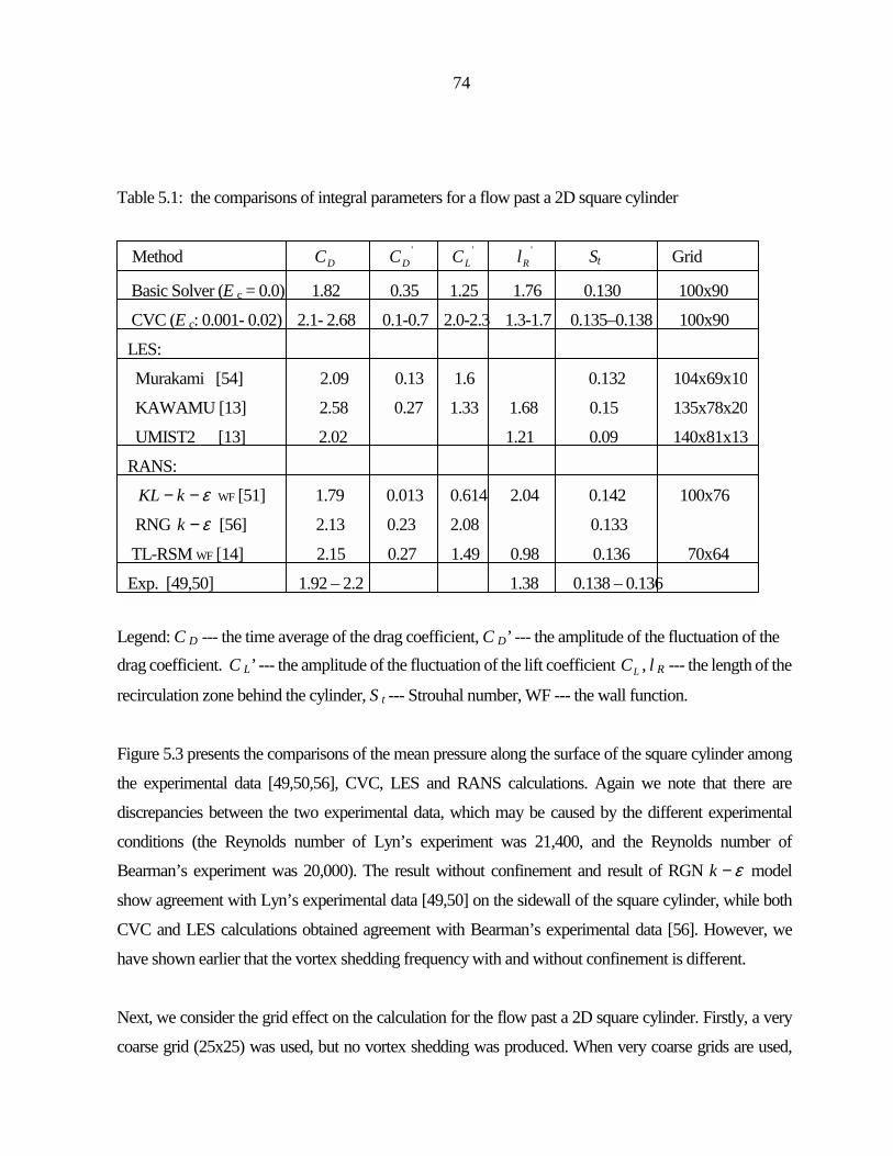
74

Table 5.1: the comparisons of integral parameters for a flow past a 2D square cylinder

Method DC 'DC '

LC 'Rl St Grid

Legend: C D --- the time average of the drag coefficient, C D’ --- the amplitude of the fluctuation of the drag coefficient. C L’ --- the amplitude of the fluctuation of the lift coefficient LC , l R --- the length of the

recirculation zone behind the cylinder, S t --- Strouhal number, WF --- the wall function.

Figure 5.3 presents the comparisons of the mean pressure along the surface of the square cylinder among

the experimental data [49,50,56], CVC, LES and RANS calculations. Again we note that there are

discrepancies between the two experimental data, which may be caused by the different experimental

conditions (the Reynolds number of Lyn’s experiment was 21,400, and the Reynolds number of

Bearman’s experiment was 20,000). The result without confinement and result of RGN ε−k model

show agreement with Lyn’s experimental data [49,50] on the sidewall of the square cylinder, while both

CVC and LES calculations obtained agreement with Bearman’s experimental data [56]. However, we

have shown earlier that the vortex shedding frequency with and without confinement is different.

Next, we consider the grid effect on the calculation for the flow past a 2D square cylinder. Firstly, a very

coarse grid (25x25) was used, but no vortex shedding was produced. When very coarse grids are used,

Basic Solver (E c = 0.0) 1.82 0.35 1.25 1.76 0.130 100x90

CVC (E c: 0.001- 0.02) 2.1- 2.68 0.1-0.7 2.0-2.3 1.3-1.7 0.135–0.138 100x90

LES:

Murakami [54] 2.09 0.13 1.6 0.132 104x69x10

KAWAMU [13] 2.58 0.27 1.33 1.68 0.15 135x78x20

UMIST2 [13] 2.02 1.21 0.09 140x81x13

RANS:

ε−− kKL WF [51] 1.79 0.013 0.614 2.04 0.142 100x76

RNG ε−k [56] 2.13 0.23 2.08 0.133

TL-RSM WF [14] 2.15 0.27 1.49 0.98 0.136 70x64

Exp. [49,50] 1.92 – 2.2 1.38 0.138 – 0.136

75

the vortices in the forward corner cannot be formed, so no vortex shedding results. In this situation,

vorticity confinement cannot help because vorticity confinement lets the velocity profile get fuller than

without confinement, and no vortices are formed in the forward corners. As a result, no vortex shedding

occurs. When the grid gets finer, the vortex shedding can be produced, but the overall good agreement for

the flow cannot be obtained unless the grid gets finer. Table 5.2 presents the comparison of the results of

two different sets of grids for the flow past a 2D square cylinder.

From Table 5.2 we see that for the coarser grid, the vortex shedding frequency is closely produced; the

amplitudes of the drag and lift coefficient fluctuations are also good. However, the length of the

recirculation zone is a little shorter than the experimental one, and the drag coefficient is much higher than

that of the experiment. If we compare the results with the results of RANS calculation and some LES

results presented in Table 5.1, the result for the coarser grid (50x50) would be reasonable. When the grid

gets finer, 100x90, the computed overall flow field is even better. Therefore, as the grid size is changed,

some characteristic parameters such as the vortex shedding frequency do not change, but the other

characteristic parameters such as the drag coefficient are affected. Overall, the fine grid CVC computation

produces results as good as state of the art LES calculations on much finer grids.

76

Figure 5.2: Time average-velocity U along the centerline of a 2D square cylinder

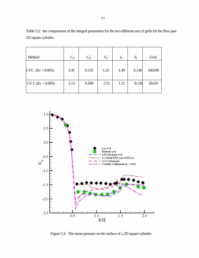
77

Table 5.2: the comparisons of the integral parameters for the two different sets of grids for the flow past

2D square cylinder.

Method CD CD’ CL

’ lR St Grid

CVC (Ec = 0.005) 2.41 0.135 1.25 1.49 0.138 100x90

CV C (Ec = 0.005) 3.13 0.500 2.51 1.21 0.130 50x50

Figure 5.3: The mean pressure on the surface of a 2D square cylinder.

78

5.3 Calculation of a Flow Over a Surface-Mounted Cube in a Plate Channel The flow pattern past a surface-mounted cube on the floor of a plate channel has a very complicated

nature in spite of the simple geometry. The flow involves multiple separation at different locations

including the front corners on the roof, the sidewall and in front of the cube. According to the flow

patterns sketched in Figure 1.3f [4,5], the main separation vortex and secondary ones were formed in

front of the cube. The main vortex is bent as a horseshoe vortex and convects down stream into a wake

around the cube with converging-diverging characteristics. Directly downstream of the leading edge on

the two sides of the cube, two corner vortices are formed at the junction of the channel floor and base of

the cube, extending downstream to the corner vortices after the cube. These vortices join at the symmetry

plane to form a closed arch behind the cube. The interactions among the horseshoe vortex, the corner

vortices behind the cube and the impinged mixing-layer in the wake dominate the flow structure for the

flow around the cube. The separation in front of the cube is characterized by bimodal behavior. That is, in

one mode, high-inertia fluid is deflected back upstream in the form of jet by the front wall. This part fluid

travels against the pressure gradient and rolls up to form up to four vortices. In the other mode, the other

part of the fluid goes downstream around the cube and forms a horseshoe vortex.

We attempted to simulate the flow past a surface-mounted cube in the plate channel with a coarse

Cartesian grid 32x24x24. 32 grid points were distributed within ten times of the cube dimension in the

free stream direction; 24 grid points were arranged within 7 and 2 times cube dimension in the span-wise

and lateral direction, respectively. The cube was located at the center of the computational domain. In

order to get enough resolution near the floor of the channel and the cube wall, the grid was stretched and

clustered near the floor of the channel and the cube wall. After 3-5 grid lines were stretched, the rest of the

grid lines were distributed uniformly. The grid lines are stretched according to the following formulation:

)( 211 −−− −+= iiii xxxx α , (5.3)

where i is the index in one of the Cartesian coordinates. In the present study, the value of the ratio α was

1.15 - 2.2, which was chosen in such a way that the grid lines were distributed as smoothly as possible.

The distance between the first grid line to the floor and the wall of the cube was 0.03 in the present study.

The grid on the symmetry plane is presented in Figure 5.4. A 1 / 6 power law of the velocity profile with

79

the maximum velocity value located at the center of the channel was used as the inlet boundary condition.

The convection boundary condition was used at the exit of the domain. The pressure at the exit boundary

was extrapolated from the closest interior points. No-slip boundary conditions were used on the wall of

the cube and the floor of the channel where the pressure is the only contribution to the numerical flux. A

parabolic approximation was used to get the pressure at boundary points from the closest interior points.

The cell-centered finite volume central-difference scheme was used with Cartesian velocity components.

In order to obtain oscillation-free solution, the matrix dissipation model MDM (2) described in Chapter 2

Reattachment on the top

X rX rX rX r

Separation in front of the cube Rear stagnation point

X f X R

Figure 5.4: The grid layout on the symmetry plane of a cube.

was used. The dissipation parameter E d was the standard value 0.5. The value of the confinement

parameter is set to 0.02, which was the value tuned for the calculation of the flow past a 2D square cylinder. The primitive variables ),,,,( pwvuρ at the face of grid cell are needed to evaluate the flux and

80

the dissipation matrix. The parabolic interpolation [52,53] for primitive variables was used to calculate the

values at either side of the cell interface. After averaging the two values we get the values of the primitive

variables at the cell interface. We also used a limiter (presented in Chapter 2) to prevent oscillations.

Figure 5.5 presents the streamline comparisons on the symmetry plane and near the floor of the channel

among CVC, LES, RANS calculations [13] and the experiments [4,5]. The time-averaged streamlines are

presented for experiment and LES. The streamline distribution calculated by vorticity confinement and

LES [57] on a plane parallel to the back face of the cube at 0.1 step size of the cube dimension are

compared in Figure 5.6. Various separation lengths defined in Figure 5.5 are summarized in Table 5.3.

The present calculated length of the separation zones in front of the cube and behind the cube and the

thickness of the separation zone on the roof of the cube are close to the experimental ones. From the

Figure 5.5, Figure 5.6 and Table 5.3 we see that the complicated vortex-dominant flow around the cube

was simulated very well using vorticity confinement. On the other hand, the standard ε−k model with the wall function predicted the primary front separation point ( fX ) too close to the cube while the

ε−− kTL model gives good agreement with the experiment for fX . The ε−k model with wall

function produced a much short separation region with unrealistic reattachment on the roof. When the KL

modification is used in the ε−k model, a much longer separation region on the roof is produced with no

Table 5.3: the comparisons of the global parameters between the preset study and the Ref. [13] for the

flow around a surface-mounted cube

Method Key X f X r X R Grid CVC 0.98 1.52 32x24x24

LES [13] UKAHY3 Smag. 1.29 1.70 165x65x97

LES [13] UKAHY4 Dyn. 1.00 1.43 165x65x97

LES [13] UBWM2 Smag. 0.81 0.837 1.72 144x58x88

RANS [13] ε−− kStd WF 0.65 0.43 2.18 110x32x32

RANS [13] ε−− kKL WF 0.64 2.73 110x32x32

RANS [13] ε−− kTL 0.95 2.68 142x84x64 Exp. [4,5] 1.04 1.61

Note: The Reynolds number in the experiments [4,5] is about 510 .

81

reattachment, but the separation bubble is still too thin compared with the observation in the experiment

[4,5]. The KL version ε−k model produced a longer separation region on the roof. The ε−k Model

with TL approach and KL modification gave better agreement with the measured in the experiment on

the roof region, but the center of the bubble moved to too far down stream. All RANS calculations with

ε−k model predicted a separation zone behind the cube that was too long. The standard ε−k model

with the wall function produced about 35 0/0 longer separation zone behind the cube than the

experimental one. The ε−k model with the TL and KL modifications enlarged X R further, giving the

most excessive length 110 0/0 longer separation zone behind the cube than that measured in the

experiment. The CVC and LES clearly did a better job. Vortex shedding from the sidewall of the cube

was observed in experiments [4,5]; such vortex shedding can contribute greatly to the momentum

exchange in the wake and therefore can significantly shorten the separation zone behind the cube. Even

though there was no clear vortex shedding found in CVC and LES calculations [13], the resolution of

large scale unsteady vortical motions seems to produce the correct effect.

Figure 5.5 shows that the horseshoe vortex is generally produced quite well by the different methods.

LES calculations and ε−− kTL model captured the converging-diverging behavior of horseshoe vortex,

but CVC and the ε−k model with the wall function did not produce this feature. CVC predicted the

correct separation length behind the cube, but the ε−− kTL model produced the separation length that

was too long.

Figure 5.6 shows that both CVC and LES calculations captured the strong vortical motion associated with

the horseshoe vortex and its interaction with the corner vortices behind the cube. In our calculation, we

found that horseshoe vortex center moves upward away from the floor of the channel in the down stream

direction.

Figure 5.7 presents the comparison of the streamline distributions on the floor of the channel between

confinement and without confinement. The solution without confinement did not captured the corner

vortices behind the cube. Figure 5.8 presents the comparison the streamline distribution on a plane

parallel to the back face of the cube and at 0.1 step size of the dimension of the cube. The solution without

confinement captured the horseshoe vortex very poorly.

82

Figure 5.9 shows the comparison among CVC, LES [58] and the experiment [4,5] for the vertical profiles

of mean velocity component U at several locations on the symmetry plane. The results with confinement

show slighter better agreement with experiment than LES [58] on the roof region, and similar agreement

wit LES downstream of the cube. Although the results without confinement for the velocity profile on the

roof region are reasonable, the results elsewhere as shown in Figures 5.7 - 5.8 indicate poor agreement.

Next we consider the grid effect for the calculation of the flow past the 3D surface-mounted cube. A finer

grid 51x35x40 was used. Figure 5.10, Figure 5.11 and Figure 5.12 present the comparison of the

streamline distributions calculated with two sets of grids on a plane parallel to the back face, on the floor

of a channel and on the symmetry plane. From these figures we see that the results with the finer grid are

generally qualitatively closer to the experimental results and the computed results of LES. From the

streamline distributions on the floor we see that the results of the finer grid displayed the converging-

diverging behavior of the horseshoe vortex, but the result of the coarser grid just has a simple pattern. The

streamline distribution with the finer grid on the plane parallel to the back face is much closer the flow

pattern computed using LES. Furthermore, from the streamline distributions on the symmetry plane, we

see that the separation bubble on the top of the cube for the finer grid is larger than that of the coarser grid.

The velocity profiles on the symmetry plane are presented in Figure 5.13. This figure quantitatively

compares the two computed results of CVC with two different grids to the experimental results and the

computed results of LES. From this figure we see that the velocity profiles of the finer grid are much

closer to the experimental results in the near wall region. This is the result of more grid points arranged in

the boundary layer. However, the profile in the core region does not seem to improve and degrades

slightly. This behavior may be explained by the computed results of the flow over a 2D flat plate using

CVC in Chapter 7.

83

Figure 5.5: The comparisons of the streamline distributions on the symmetry plane and on the floor of

the channel. All the results but CVC are from Rodi [13].

84

CVC

LES [57]

Figure5.6: The comparisons between CVC and the LES calculation [57] for the streamline distributions

on the plane parallel to the back face at 0.1step size of the cube dimension.

85

Figure 5. 7: Comparison of the streamline distributions with and without CVC on the plane near the floor

of the channel. Grid 32x24x24.

86

Figure 5. 8: Comparison of the streamline distributions with and without CVC on the plane which is at

0.1 step size of the dimension of the cube and parallels to the back face of the cube. Grid: 32x24x24.

87

U∞

0.0 1.0 X/H

Figure 5.9: The comparison among CVC, LES [58] and the experiments [4,5] for the mean velocity

component U at several locations on the symmetry plane.

88

Figure 5.10: The comparison between CVC and LES calculation [57] for the streamline distributions on

the plane parallel to the back face at 0.1 step size of the cube dimension.

Legend: (a) LES [57], (b) CVC with grid 51x35x40, (c) CVC with grid 32x24x24.

89

Figure 5.11: The comparison among experiment [4,5], LES-D [13], and CVC for the streamline

distributions on the floor of the channel.

Legend: (a) experiment [4,5], (b) LES-D [13], (c) CVC with grid 51x35x40, (d) CVC with grid

32x24x24.

90

Figure 5.12: The comparison among experiment [4,5], LES [57], and CVC for the streamline

distributions on the symmetry plane.

Legend: (a) experiment [4,5], (b) LES [57], (c) CVC with grid 51x35x40, (d) CVC with grid 32x24x24.

91

(a)

(b)

Figure 5. 13: The velocity profiles on the symmetry plane. Experiment --- Refs.[4,5]; LES --- Ref.[58].

92

5.4 Conclusions

The numerical simulation for the turbulent flows past a 2D square cylinder and a 3D surface- mounted

cube are among the most difficult problems in current CFD, since the flow patterns are very complex and

featured by bimodal, multiple separations with steep streamline curvature, arch and corner vortices

behind the cube, and for two-dimensional case, periodical vortex shedding.

The comparisons of results from CVC, LES and RANS calculations for the flow around a 2D square

cylinder presented above showed that CVC calculation gives an entirely satisfactory qualitative picture of

the flow field. The standard ε−k model produced very poor results due to its under predicting the

unsteady large-scale vortical motions that may be explained by its excessive “turbulence production”

(modeled dissipation) in the front stagnation region. The TL and KL modification produced improved

results. The excessive “turbulence production” is removed by using RSM, but this will give over

prediction of the unsteady vortical motions.

The LES calculations gave better results than did the RANS calculations for the flow around a 2D square

cylinder, but the price to be paid for these results was very high. According to Ref. [13], The LES-

UKAHY2 calculation took 73 hours on a SNI S600/20 vector computer, but RANS calculation with the

wall function took 2 hours and TL approach took 8 hours on the same computer, while CVC calculation

took about 4 hours on PC with a 733 MHz Pentium III Processor.

For the flow over the 3D cube on the floor of a channel, the flow field calculated with CVC was in

generally good qualitative agreement with the experimental results and LES calculations. However, the

detail of the converging-diverging behavior of the horseshoe vortex near the floor and behind the cube

was not predicted on the coarse grid. Grid refinement did capture this detail with CVC.

In general, CVC produced much better agreement with experimental data than RANS calculations, which

completely failed to predict the correct separation length behind the body. The quantitative agreement for

axial velocity profiles for the CVC calculations was excellent and compared very favorably with the best

of the LES calculations.

93

For the calculation of the flow past a cube, LES-UKAHY2 took 160 hours on SNI S600/20 vector

computer while RANS with TL model took 6 hours and the standard ε−k model with the wall function

only took only 15 minutes on the same computer [13], but CVC with 32x24x24 grid points just took

about 40 minutes on PC with a 733 MHz Pentium III processor. In addition, LES calculations must use

very fine grids (about one million) to obtain reasonable solution for 3D calculations. However, in the

present study, by using CVC we obtained a reasonable solution with just about 2% grid points of the LES

calculations; as a result, much less computer resource was used. With the overall performance and the

computer resource required, CVC looks to be very promising for solving the realistic engineering

problems such as the flows around tall buildings, bridges and automobiles, etc. However, further study

and testing are necessary to evaluate solution accuracy and reliability.

From the calculations we observed that the value of the confinement parameter played important roles in

deciding the vortex shedding frequency and the drag coefficient for the flow past a 2D square cylinder.

Furthermore, the vortex shedding frequency without confinement was predicted smaller by 6 % - 13 % of

the measured range of the experiments and no vortex shedding occurred when a very large value of the confinement parameter is employed, ( 5.0=cE was tested in the present study). In addition, the drag

coefficient increases as the value of the confinement parameter increases. The drag coefficient without

confinement was predicted smaller by 5 % - 17 % of the measured range of the experiments. On the other hand, if 01.0001.0 −=cE is chosen, the drag coefficient will fall in the measured range of the

experiments.

Finally, we consider the issue of grid convergence. For the calculation of the flow past the 2D square

cylinder, we used two sets of grids. One was 50x50; the other was 100x90. We believe that we obtained

the grid convergent solution with the finer grid. However, for the calculation of the flow over the 3D cube

mounted on the floor of a channel, we have not been able to test finer grids because very large computer

resources are needed, and we may not have obtained the grid convergent solution for this case.

94

Chapter 6 Parallel Computation for the Flow past a 3D Surface-Mounted Cube Using Domain- Decomposition Algorithms

6.1 Introduction

Turbulent flows around three-dimensional (3D) obstacles are common in nature and occur in many

applications including flow around tall buildings, vehicles and cooling flows around computer chips. The

sketched flow pattern for the flow past a cube mounted on the floor of a plate channel is presented in

Figure 1.3f. Understanding and predicting the properties of the flows are necessary for effective,

economical and good engineering designs. Experimental techniques are expensive and often provide data

that is not sufficiently detailed. With the advent of supercomputers it has become possible to investigate

these kinds of flows using numerical simulations.

As we discussed in Chapter 1, a number of approaches to computer prediction of flows past 3D obstacles

have been proposed and used. One of the approaches is solving Reynolds-Averaged-Navier-Stokes

(RANS) [13,15] equations with a variety of turbulence models. Another approach is Large Eddy

Simulation (LES) [13,57,58], in which the large scales of motion are computed explicitly, while the small

or sub-grid scale motions are modeled. In the present computation, we used Euler equations with

Compressible Vorticity Confinement (CVC) approach. The complicated turbulence models of RANS

95

and huge computation of LES are both avoided in this approach, and from discussion in Chapter 5, we

see that it should suffice to capture the large turbulent structures present in the flows.

6.2 Computer Requirements

If the LES approach is used to simulate the turbulent flows past a 3D surface-mounted cube in a plate

channel, it is estimated that the grid points will have to be about one million in order to obtain

“engineering-accuracy” prediction of the surface pressure and the overall wind force over the cube.

Furthermore, about 100,000 iterations will be required in order to resolve the unsteady motion of the

turbulent flow structures. Supposing 10,000 operations per point per iteration, then about 1015 operations

will be required per problem. In 1990, H. Werner and H. Wengle used LES to simulate the turbulent

flow over and around a cube mounted on the bottom of a plate channel using 144x96x56 (766,364) grid

points [58]. In 1996, K. B. Shah and J. H. Ferziger performed the LES for a 3D surface-mounted cube

with 196x64x94 (1,179,646, more than one million) grid points [57]. If a sequential code was used to run

this kind of problem, both run time and memory storage could be problematic. So in this chapter an

effective fast parallel computation will be developed using domain-decomposition algorithms.

6.3 Parallel Algorithms

From the long-term viewpoint, parallel computing is the solution for intensive computer simulations in

CFD research and its engineering applications. Parallel computing offers the promise to provide the

massive computational resources that CFD requires. However, the practical achievement also relies on

the parallel algorithms and numerical methods that play important roles in the computation. Domain

decomposition is the most natural and popularly used approach for parallel computing in CFD. In fact,

decomposition of physical or computational domains has been used in CFD for years because of the

benefits of allowing physically zonal modeling and saving storage in implicit procedures. For most

explicit solution methods, implementation of domain decomposition is straightforward. Some effort must

be made, however, to minimize synchronization and communication overhead. On the other hand, load

balancing is another very important factor that must be considered for achieving high performance

96

parallel computing in CFD. The effects on performance of the synchronization and load balance will be

reported in the last part of this chapter.

6.3.1 Domain Decomposition Algorithm Using One-To-One Scheme [59]

The computational domain is divided into a number of equal size sub-domains in the stream direction

(the same as the number of processors in use), and the computation within each of the sub-domains is

mapped onto one of the processors available, hence the name of the algorithm. Here “equal-size” means

that the number of mesh points of each sub-domain is about equal to each other. Within each sub-domain, updating of the flow variables wvu ,,,ρ and p is done sequentially, whereρ is the density in the flow

field, ),,( wvu is the velocity component in x, y and z direction, respectively, in Cartesian coordinates.

The values of the flow variables at boundary points of each sub-domain are transferred from the closest

two neighbors. Only two communications are required per sub-domain per iteration. There also have

been two other domain-decomposition algorithms available for CFD. One has six way communications if

the computational domain is divided into sub-domains in x, y, and z directions simultaneously [60]. The

other has four way communications if the computational domain is divided into sub-domains in x and y

directions simultaneously [60]. The algorithm used in the present research has the minimum

communication cost among these three methods. Furthermore, the load balance can be achieved more

easily with the domain being divided into sub-domains just in one direction.

In conclusion the domain decomposition algorithm using the one-to-one scheme is given below:

Step 1: Decompose the computational domain into number of processors N in the stream direction.

Step 2: Map each sub-domain onto one of the processor available.

Step 3: Do n = 1, N_iteration in parallel.

Step 3_1: Let all the processor do each iteration n within each sub-domain.

Step 3_2: Let all the processor P1, P2, … PN do synchronization at the end of each iteration.

Step 3_3: Let all the processors do communication between the two closest neighboring

processors.

End do.

97

6.3.2 Domain Decomposition Using Pipeline Scheme [59] The manner used for domain decomposition for a pipeline scheme is the same as the one-to-one scheme,

but the communication and implementation is completely different. First, let one of the processors

compute an iteration over the entire domain one sub-domain by one sub-domain so that when it finishes

one sub-domain or begins to compute a new sub-domain, let another processor start working on it at the

new iteration, and so on so forth. If the domain is decomposed into N sub-domains, and N number

processors can be available, let N processors collaborate to compute the entire domain, after the N-th

processor finishes the last sub-domain, the first processor should begin to calculate the (N+1)-th iteration.

Obviously, the processor needs the data of the previous iteration, so the communication is needed

between the processors that perform the current iteration and the previous iteration. In order to

communicate in the consistent way with the pipeline scheme, the processor should transfer the data for

each sub-domain into the processor that will perform the same sub-domain at the next iteration. In this

fashion the data gets communicated in something like the manner with which 4 people collaborate to do a

relay race game. When one person finishes a quarter of a circle, he or she transfers the baton to another

person who is waiting there and after he or she gets the baton, he or she continues to run the second

quarter of the circle, so on and so forth until they finish the race.

In conclusion, the domain decomposition algorithm using the pipeline scheme can be given as follows:

Do n = 1, N_iteration, N_processor.

Step 1: Let processor 1 start to compute the entire domain from sub-domain 1 to sub-domain N at

time step n.

Step 2: If (processor 1 finishes the calculation of the first sub-domain) Let processor 2 start to

compute the entire domain at time step n+1.

Step N: … so on so forth until to processor N.

End Do.

6.3.3 Synchronization One of the very important issues for parallel CFD is the synchronization. For unsteady problems,

synchronization must be enforced at the end of each iteration or at the beginning of each iteration to

98

guarantee accuracy, because the data at the boundary points and the data between n and n+1 time steps

are dependent upon each other. But this must be paid off for run time overhead. On the other hand, for

steady problem, synchronization is not performed at every iteration, but may be performed at every 10 or

20 iterations. That will save the time for synchronization. In the present research, we ignored the

synchronization in pipeline scheme to study the effect of synchronization on the performance of the

parallel computation.

6.3.4 Load Balancing

Load balancing is related to the size of the sub-domain in domain decomposition using the one-to-one

scheme, because the processor that corresponds with the sub-domain within the cube will be in idle status.

This problem may be solved by letting the size of the sub-domain that corresponds to this part of the flow

field increase so that the work to be done in the sub-domain inside the cube is about equal to that in the

sub-domain outside the cube. However, in order to study how load unbalancing impacts on the

performance of the parallel computation, we decompose the domain into sub-domain with about equal

length in the stream direction. When the number of sub-domain increases, the size of each sub-domain

will decrease, and load unbalancing will increase. The effects on performance of load unbalancing will be

reported in the last part of this chapter.

6.4 Implementation Issues

The whole implementation was completed using Fortran 90 and Message Passing Interface (MPI) [61]

on a Beowulf computer. The implementation includes the numerical methods along with the

communication and synchronization approaches. In this section, we will discuss how to implement the

communication between processors and processes and how to synchronize all the processors and

processes. The original sequential code was written in Fortran 90. Fortran 90 is a good language for

parallel scientific computation. There are many built-in procedures that can help to achieve high

performance. In the present research the original Fortran 90 code was modified into parallel code using

MPI.

99

The communications between the two closest processors / processes are implemented using MPI. The

MPI_SENDRECV is used to implement the data shift in the two neighboring processors for one-to-one

scheme to prevent the dead lock that may be caused in the communications. MPI_SEND and

MPI_RECV both were used in the two closest processes (the process at time step n and the process at

time step n+1) in the pipeline scheme. For one-to-one scheme, MPI_GATHER is called to gather the data

from each processor to calculate the residual of the whole domain and stores the data for visualization of

the whole computation domain, and MPI_BCAST is used to broadcast the data from the root processor

(with zero process id) to each of the other processors for initializing the flow variables. The pipeline

scheme calculates the residual in each processor, so that no data gather will be performed. Furthermore,

the data initialization for flow variables is needed just for the processor that begins the calculation in the

first iteration. So no MPI_GATHER and MPI_BCAST are needed to do the data initialization for

pipeline scheme. Just one MPI_BARIER is called to implement the synchronization of all the processes

at end of each iteration for the one-to-one scheme.

6.5 Numerical Experiment Results and Analyses

In this section, we present all the numerical experiment results of the parallel computation using the

methods described above.

The Speed Up and Efficiency are defined as Speed Up = T 1/T p and Efficiency = Speed Up / p. Here, T 1

is the CPU time for one node to finish the whole computation (using the same code and memory space).

T p is the CPU time for p nodes to collaborate to complete the parallel calculation.

The parallel computation was performed with 100 time steps and 32x24x24 Cartesian grid points. This

set up is just for purpose of testing the program. In an actual computation, many more iterations and

many more grid cells may be required.

100

The Speed Up curve is presented in Figure 6.1, the Efficiency curve is presented in Figure 6.2, and the

performance curve in term of CPU time is shown in Figure 6.3.With the curves presented here we can

discuss that how the type of scheme, synchronization, the size of sub-domain and load unbalancing

impact on the performance of the parallel computation.

6.5.1 Speed Up and Efficiency vs. Scheme and Synchronization With the Speed Up curve presented in Figure 6.1, we can see that the slope of the Speed Up of one-to-one

scheme with synchronization is much lower than the pipeline scheme without synchronization. At the

same time the efficiency curve presented in Figure 6.2 shows the efficiency of pipeline is much higher

than that of the one-to-one scheme. Both the type of the scheme and synchronization played a very

important role in this parallel computation. Synchronization is especially important; it shows more

importance because the work done in one-to-one scheme and pipeline scheme are not substantially

different. The data transferred in pipeline scheme from one processor that performs the calculation at time

step n to the processor which performs the calculation at time step n+1 is much more than the data

transferred in one-to-one scheme between the closest two neighboring processors. Because in the pipeline

scheme the data transferred are the whole data in each of the sub-domain while the data transferred in the

one-to-one scheme are just the data at the boundary points. So the communication time in the pipeline

scheme should be longer than that taken in one-to-one scheme. Hence the synchronization overhead in

one-to-one scheme dominates the total overhead in the computation. This observation is the same as that

reported in other parallel CFD computations [59].

6.5.2 Efficiency vs. Load Balancing The efficiency curve presented in Figure 6.2 shows that the efficiency for the one-to-one scheme

decreases very sharply as the number of processors increases. One of the reasons could be

synchronization. Another very important reason is the load unbalancing. As the number of processors

increases, the number of sub-domain also increases. The domain is divided into equal-size sub-domains

with the same number of processors, so the size of the sub-domain will decrease as the number of sub-

domains increases. The grid used is a Cartesian grid, the sub-domain inside of the cube is still counted as

sub-domain, but the work done there is much smaller than the work done in the sub-domain outside the

cube. So the processor that performs the calculation of the sub-domain inside the cube idled most of the

101

time; therefore, the load is unbalanced. When the number of processors increases, the load unbalancing

gets much worse. One of the procedures that can fix this problem is to increase the size of the sub-domain

inside the cube letting the work to be about the same as that done in the sub-domain outside the cube. But

here we have divided the domain into equal size sub-domain in order to study the effect on the

performance of the parallel computation by the load unbalancing. Therefore, in addition to

synchronization, load balancing is another very important factor for obtaining high parallel performance.

6.5.3 Performance in Term of CPU Time The CPU time curve presented in Figure 6.3 shows smaller difference between the one-to-one scheme

with synchronization and pipeline scheme without synchronization compared with efficiency difference

between the two schemes. The load unbalancing inside the cube left some of the processors idle.

However, the time for the processor to perform its computation in the sub-domain outside the cube

should be the same if the number of processors used is the same for two schemes. The only difference

comes from the differences of the overhead due to synchronization and communication. So the results

obtained are reasonable. The same conclusion was obtained by other parallel computation [59].

6.6 Conclusion

The performance of parallel computation strongly depends on the specific algorithms and the actual

implementation. The type of the scheme, the size of the sub-domain, synchronization and load balancing

all play very important roles and are correlated in achieving high parallel computing performance. For the

types of problems that we were solving the pipeline scheme without synchronization achieved the best

performance in a simple domain and a structured grid.

102

Figure 6.1: Speed Up vs. type of scheme and synchronization.

Figure 6.2: Efficiency vs. load balancing.

103

Figure 6.3: Performance in term of CPU time.

104

Chapter 7 Fundamental Properties of Compressible Vorticity Confinement (CVC)

Some applications of Compressible Vorticity Confinement (CVC) to complex vortex-dominant flows

were presented in Chapters 3 through 6. However, a number of fundamental questions have arisen: Why

does CVC work so well for turbulent flows? What is the numerical accuracy for CVC? What are the

limitations for using CVC? In this chapter, we will try to give some preliminary answers for these kinds

of questions and attempt to give some insight to the fundamental properties of CVC.

7.1 Turbulent Boundary Layer Over a Flat Plate

Almost all engineering problems in fluid dynamic applications are turbulent. The flow past a square

cylinder and the flow over a surface-mounted cube on the floor of a plate channel are complicated

turbulent flows with massive separation. The results presented in Chapter 5 are generally in good

agreement with experiments and state-of-art computations with RANS and LES methods despite the fact

that only an Euler solution with the grid spacing appropriate for an inviscid flow was used with a no-slip

boundary conditions enforced on solid walls. One large difference between CVC and LES calculations is

the number of grid points. The grid points (32x24x24) we used for the flow over a cube were about 1 / 60

the number of grid points (172x64x76) used by Shah and Ferziger [57] and about 1 / 40 the number of

grid points (144x72x58) used by Werner and Wengle [58]. An important question is now why did CVC

obtain good agreement with the experiments and LES using such a coarse grid?

The turbulent flow over a flat plate is much simpler than the turbulent flow past a 3D cube in a channel or

the flow over a 2D square cylinder. The results of this simple case may help to understand the

105

complicated situations. In order to gain insight into the behavior of the method, we considered the flow

over a 2D flat plate.

The calculations are performed using our basic inviscid flow solver, with the confinement term added

along with a no-slip boundary condition, using a grid adequate to model the inviscid phenomena. Note

that we are not advocating this approach to produce accurate boundary layer results. We are performing

this calculation to try to understand the results presented for the vortex dominated flows in the preceding

chapters. The basic solver MDM (2) and scalar vorticity confinement with dissipation parameter E d = 0.3

were employed in this calculation. We chose this value because in most of our applications we used this

value or a value that was close to it. On the other hand, we will use different values of the confinement

parameter to test the effects of the value of the confinement parameter on the velocity profile of the flow

over a 2D flat plate. Furthermore, different grid sizes in the normal direction of the flat plate and along the

plate were used to test the effect of the grid size on the velocity profile.

The flat plate is 1 ft long (L = 1ft), and the free stream is the air at sea level with Mach number 0.1, at

which the Reynolds number approximates 200,000. Uniform free stream conditions are imposed at a

distance L/4 upstream of the plate, and L/2 above the flat plate. No-slip conditions are applied on the

plate and the flow variables are extrapolated downstream at the exit of the computational domain in

stream wise direction.

The coordinates consist x and y; x is the coordinate in stream direction with the origin at the inlet and y is

the coordinate in the normal direction with the origin at the flat plate. In order to present our results, there

are two scales which may be used to scale the vertical coordinate y. One is the thickness of a laminar

boundary layer over a flat plate, which is written as follows:

eL U

xνδ 0.5≈ , (7.1)

the other is the thickness of a turbulent boundary layer over a flat plate, which may be approximated as

follows:

106

5/1)/(375.0ν

δxU

xe

T ≈ , (7.2)

where eU is the velocity at the outer edge of the boundary layer, ν is the kinematic viscosity in the flow.

We use Blasius solution as the “exact” solution of the laminar boundary layer, and use 1/8 power law

profile as the turbulent boundary layer solution. The 1/8 power law is written as follows:

81

)(Te

yUu

δ= . (7.3)

First, we computed the flow on a 100x25 grid and a 200x25 grid without confinement (E c = 0) and with

confinement (E c = 0.12) to test the effect of the confinement and the grid spacing effect in the streamline

direction on the velocity profile. Figure 7.1 presents u/U e profiles with and without confinement versus the Ty δ/ . Figure 7.2 presents u/U e profiles without confinement versus Ly δ/ . Figure 7.3 presents u/U e

profiles with confinement (E c = 0.12) versus Ty δ/ . Figure 7.4 presents the velocity profiles versus

Ty δ/ at more locations about the developmental boundary layer. With this figure we have three

important findings: (1) The velocity profile u/U e with confinement vs. Ty δ/ is fuller than the turbulent velocity

profile but resembles a turbulent boundary layer in the near wall region; (2) The velocity profile u/U e vs. Ly δ/ more closely approximates a laminar velocity

profile than a turbulent profile when confinement is turned off;

(3) The solutions at different axial locations are more “similar” to each other when

confinement is applied in the calculation. Solutions without confinement do not appear to

have any measure of this similarity property.

Next, we consider the effect of grid spacing in the normal direction by considering mesh sizes of 100x10,

100x25, 100x50 and 100x100, all with vorticity confinement, E c = 0.06. In Figure 7.5 we see that the

velocity profile evaluated at x = 2L/3 becomes slightly fuller as the mesh is refined. However, all the

profiles have very similar behavior near the wall, even the coarsest grid. The coarsest grid case somewhat

mimics the three-dimensional separated flow cases discussed in section 5.3, which had one or two grid

points in the turbulent boundary layer, but obtained an overall good approximation to the experimental

data.

107

Finally, we show the effect of confinement parameter on the velocity profile. Figure 7.6 presents the

velocity profiles u/U e at x = L/3 and a100x25 grid with a series of the confinement parameters 005.0,01.0,02.0,04.0,06.0,12.0,24.0,48.0,96.0=cE and no confinement E c = 0. From Figure 7.6

we see that increasing the confinement parameter over this range of values produces increasingly fuller

profiles until, for values beyond E c = 0.35, the velocity profile overshoots. For small values of E c, the

profile is more “laminar”, but as discussed previously, the similarity property is not well represented. However, we see that over a range in values of 24.006.0 ≤≤ cE , that at least in the near wall region,

the velocity profile is relatively insensitive to the value of confinement parameter. Over this range of

values, as shown in Figure 7.7, we believe that the current method provides a rough approximation to a

turbulent boundary layer. Then, for flows involving massive separation, the approximate boundary

solution may be accurate enough to generate a separation of large-scale structures. It is well known that

massive separation from sharp edges is dominated by the behavior of the inviscid rotational flow. Once

the structures are generated, the vorticity confinement method does a good job of computing the mainly

inviscid rotational flow.

Figure 7.1: Velocity profiles with and without confinement at two locations in the stream direction.

108

Figure 7.2: Velocity profiles without confinement at two locations in the stream direction.

Figure 7.3: Velocity profiles with confinement at two locations in the stream direction.

109

Figure 7.4: Velocity profiles of the developmental boundary layer. (a) Velocity vector distributions at different locations. (b) Velocity profiles u/U e at different locations vs. Ty δ/ .

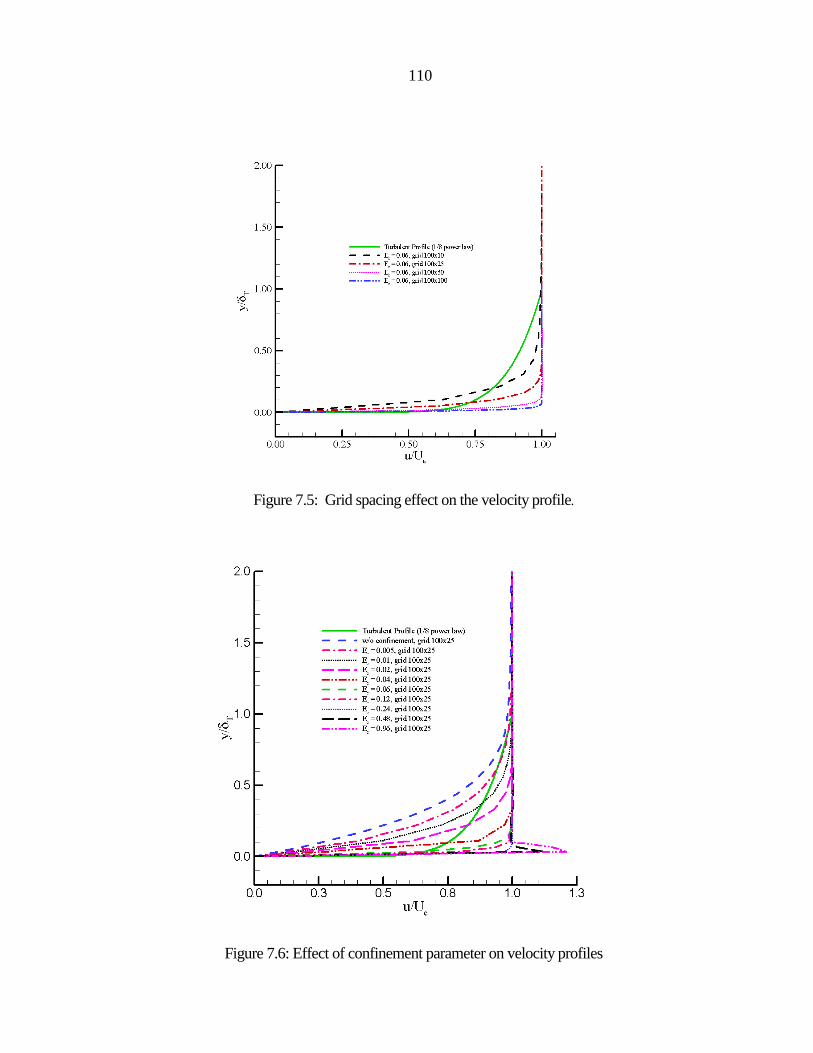
110

Figure 7.5: Grid spacing effect on the velocity profile.

Figure 7.6: Effect of confinement parameter on velocity profiles

111

Figure 7.7: Effect of confinement parameter on the velocity profile.

7.2 Supersonic Shear Layer

An inviscid supersonic shear layer flow is formed by two parallel streams, one at Mach number M = 2.4

and the other at M = 2.8. In order to show that the solution is independent of the direction of the grid, we

let the two streams flow at an angle of 30o relative to the horizontal grid line. The computational grid is a

100x100 uniform Cartesian grid. The basic solver is the MDM (2) (discussed in Chapter 2) with

dissipation parameter E d = 0.3. Figure 7.8 and Figure 7.9 show the Mach number contours. Figure 7.8

presents the result of the calculation with the vorticity confinement turned off. The dissipation of the

shear layer is obvious. Figure 7.9 shows the same computational result, but with the confinement in effect.

112

The contours indicate practically no degradation of the shear layer. Figure 7.10 presents the Mach number

profile computed using confinement meters E c = 0.3, 0.1 and no confinement E c = 0.0 along a cut line

that parallels to vertical axis. From the Mach profiles we see that without confinement the solution is

significantly degraded, and increasing the confinement parameters will sharpen the discontinuity, but

eventually develop an overshoot in the profile.

Figure 7.8: The Mach contours of inviscid supersonic shear layer. No confinement.

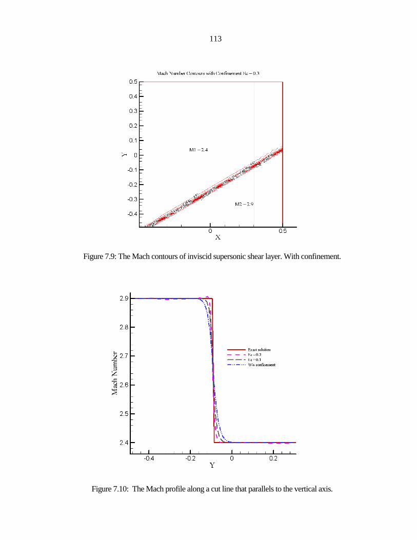
113

Figure 7.9: The Mach contours of inviscid supersonic shear layer. With confinement.

Figure 7.10: The Mach profile along a cut line that parallels to the vertical axis.

114

The effect of grid size on the classical accuracy of the solution for this problem has been investigated by

performing the calculation on three sets of grids, 200x200, 100x100 and 50x50 for E c varying from 0 to

0.3. Figure 7.11 presents the L 2 norm of the error between the computed Mach number distribution and

the exact (non-dissipated) Mach number distribution. With the analysis of Figure 7.11 we have two

findings:

(1) The error decreases as the grid size decreases when confinement parameter is fixed;

(2) The error decreases as the confinement parameter increases when the grid size is fixed.

Therefore, the effect of decreasing the grid size (increasing the grid points) is similar to increasing

confinement parameter when the grid size is fixed. This conclusion may help to explain why we could

use the very coarse grids to get good results for 3D and 2D turbulent flows. Furthermore, the conclusion

drawn above can be reached by accuracy analysis presented in Figure 7.12, which shows the slope of the log of the norm of the error with respect to the )log( x∆ . From this figure we see an improvement in the

error with increasing value of confinement parameter, with E c = 0 .3 achieving close to second-order

accuracy.

Figure 7.11: L2 error norms vs. grid size for supersonic shear flow calculations. N is the number of grid

points.

115

Figure 7.12: Slope of the log of the error L 2 norm with respect to log of grid size.

7.3 Vortex Moving with a Uniform Free Stream

Next, we consider the flowfield about a vortex moving with a uniform stream. The computational

boundary is a square domain 1x1 m2. Periodic boundary conditions are set at all edges of the domain. The

computed vortex will then pass through the grid and reappear on the other side. The initial condition of

the vortex is set up according to Povitsky and Ofengeim [8]. The tangential velocity distribution is

prescribed between an outer radius r = R 0 and a core radius r = R c. Outside R 0 the tangential velocity of

vortex is set to zero. Inside the circle with radius R c the velocity is linearly proportional to the radius r,

hence goes to zero at the center of the vortex, r = 0. The tangential velocity of the vortex can be expressed

as

≤≤+≤

=0,/

,/)(

RrRrBArRrRrU

ruc

cccθ , (7.4)

where

116

220 c

cc

RRRU

A−

−= ,

220

20

c

cc

RRRRUB

−= . (7.5)

From Eqs. (7.4)-(7.5), we see that ccR URuu

c== )(,0)0(θ , and 0)( 0 =Ruθ . The velocity θu at R c

reaches U c, the maximum velocity magnitude of the whole domain and U c is a parameter being

prescribed before calculation.

The initial vortex is imposed on a uniform free stream and the center of the vortex is located in (0,0) of the

Cartesian coordinates. In order to study the non-uniform grid effect on the solution, the grid is stretched

and non-uniformly generated. The minimum grid space is 0.0044, which is located at the center of the

domain. Then the grid space is stretched according to an exponential function, which is written as follows:

max

max

12

11

,...,2,11

1

0.10.1

)(

1

2

max

iii

ik

keem

xxmxx ii

=−

−=

=−−=

−+=

ββ

β

β

, (7.6)

where 50,5.1,5.0,0022.0 max11 max

==== ixx i β . The grid is symmetric about the x and y coordinates.

A sample grid is presented in Figure 7.13.

We performed the calculation with R c = 0.05 m, R 0 = 10 R c. The speed of sound was sma /347=∞

and U c = ∞U = 0.5 ∞a on the 100x100 non-uniform grids. The calculation was carried out with MDM (1)

and the scalar confinement described in Chapter 2, in which the dissipation and confinement parameters were set to 006.0,30.0,01.0 )4()2( === cEkk .

117

Figure 7.13: Sample grid for calculation of a moving vortex in uniform compressible flow.

The analytical solution and the initial conditions of a compressible vortex moving with a uniform free stream are presented in Appendix C. From Appendix C we see that the quantity ρω / of a vortex will be

conserved as it convects in compressible, inviscid, non-conducting fluids. Figure 7.14 presents the contours of the quantity ρω / of the flow without confinement after the vortex has passed through the

grid one cycle and approximately backed to the center of the computational domain. Figure 7.15 presents

the same calculation, but after passing through the grid ten cycles. The degree of dissipation is quite

obvious. Next, Figure 7.16 and Figure 7.17 present the results of the same calculations with the vorticity

confinement in effect. These figures are essentially identical to each other, no dissipation are shown in

these two figures.

118

The profile of the quantity ρω / along a diameter of the moving vortex is presented in Figure 7.18. From

this figure we see that the solutions without confinement looks like the solution of the Navier-Stokes

equations with the physical viscosity replaced by the numerical dissipation. However, we solved the

Euler equations; no viscosity terms exist. Therefore, the solution should not have had the dissipative

behavior similar to the solution of Navier-Stokes equations. On the other hand, the solutions with

confinement do not show the dissipative behavior of the solutions without confinement, even though the

vortex moved for ten cycles and backed to about the original place. Furthermore, the solution without

confinement decreases as the vortex moves along with the uniform free stream, until all the value of ρω / is damped out, because no “force” exists to balance the numerical dissipation. On the other hand,

the solution with confinement is approximately close to the analytical solution except that there are some wiggles at the region near cRr = , which may be caused by the interaction of the free stream and the edge

of the core of the vortex where exists a strong velocity and vorticity gradients. From this fact we may

conclude that the vorticity confinement almost cancel most of the numerical dissipation errors to conserve the quantity ρω / of the vortex.

In order to see how vorticity confinement method works on a very coarse grid, we did the same calculation on very coarse grid 12x12. The profile of the quantity ρω / with confinement along a

diameter of the vortex is presented in Figure 7.19. The solutions are actually dissipated, but essentially do

not change with time. The vortical structure is captured within 4-6 grid cells and convects without

changing the internal structure. This is our objective in design of the vorticity confinement method for

practical flow situations in which thin concentrated vortical layers persist very long distances without

significant dissipation. Actually, the conventional CFD numerical method cannot be used to obtain the

solution without significant dissipation due to dissipative error of numerical discretization. This situation

is more serious when the calculation is performed on a coarse grid. In a practical calculation, especially

for 3D flow passing through a complex geometry, fine grid calculations may be very expensive, and

computer storage may be an issue. However, with CVC, complex flow fields may be computed using

coarse grids. In addition, Hu and Grossman presented some interesting results and discussion of CVC for

a moving vortex with a uniform stream in Ref. [46].

119

Figure 7.14: Contours of the quantity ρω / of a vortex moving with a uniform free stream after one

cycle. No confinement.

Figure 7.15: Contours of the quantity ρω / of a vortex moving with a uniform free stream after ten

cycles. No confinement.

120

Figure 7.16: Contours of the quantity ρω / of a vortex moving with a uniform free stream after one

cycle. With confinement.

Figure 7.17: Contours of the quantity ρω / of a vortex moving with a uniform free stream after ten

cycles. With confinement.

121

Figure 7.18: Profile of the quantity ρω / across the diameter of a moving vortex. Finer grid 100x100

Figure 7.19: Profile along a vertical slice taken through the center of the vortex. Coarse grid 12x12.

122

The moving vortex problem also can serve as test of the numerical formulation. In Ref. [62], it was

pointed out that for large values of confinement parameter, the present formulation may increase the total

temperature of the flow. The initial investigations showed that small variations of T0 occur, and,

disturbingly, grow with iteration. It also appeared that using relatively large values of the confinement

parameter E c for the body confinement procedure exacerbated this phenomenon [62]. The initial study

indicated that the situation was improved by using a scalar implementation of the confinement, rather

than the matrix form. Secondly, the situation was also improved by completely eliminating the rate of

work done by the “body force” as it appears in the energy equation. Then a systematic procedure was

developed by considering the following conditions:

1) The present formulation, i.e., rate of work term in the energy equation and matrix confinement;

2) Rate of work term in the energy equation and scalar confinement;

3) No rate of work term in the energy equation and matrix confinement;

4) No rate of work term in the energy equation and scalar confinement.

We have repeated the computation of the vortex moving in a uniform flow with the same data previously

outlined but on uniform grid 100x100. The computation was executed for 15,000 iterations that

correspond to approximately 9 circuits. We have observed that the different formulations give almost the

same results in terms of the vortex confinement. We can conclude that all the formulations are effective in

confining the vortex. However, the total temperature changes. We computed the average total temperature, 0

avgT , defined as follows:

∑ ∑−

=

−

=−−=

1

1

1

1

0,

maxmax

0max max

)1)(1(1 i

i

j

jjiavg T

jiT , (7.3)

where 0

, jiT indicates the total temperature at each cell center (i , j), and maxmax , ji are the maximum

number of grid points in the x and y directions, respectively. Figure 7.20 presents the evolution of 0avgT

during the computation. The formulation in 4) above, gives an almost constant total temperature trend,

which follows from the physics of the problem. The introduction of the rate of work in the energy

equation determines increases of the total temperature. Increases can also be observed for the matrix

confinement with no work inserted in the energy equation. Indeed, the matrix multiplication causes the

fifth term of the vector S to be nonzero, although no work is explicitly inserted in the energy equation. For

123

computing smaller vortices (with respect to the grid size), larger values of the vortex confinement

coefficient E c are required. Noting that the total temperature increase is roughly proportional to E c.

Significant errors may be expected if the work term is inserted into the energy equation and if the matrix

confinement is applied. Errors as large as 35% have been experienced in the body confinement

computations [62]. Indeed, this computation required E c values two orders of magnitude larger and the

observed total temperature errors were approximately two orders of magnitude larger.

The second case that we calculated for investigating the effect of work done by the “body force” on the

total temperature is the flow over a flat plate. We repeated the same calculation of the flow over a flat

plate using the systematic procedures outlined above and a Cartesian grid 200x25. The confinement

parameter in this case E c = 0.06. Figure 7.21 presents the velocity profiles at 2L/3. From this figure we

see that all the four confinement procedures produced the same confinement effect for turbulent velocity

profile. However, Figure 7.22 shows that the work rate inserted in energy equation increases the total

temperature. The tendency of increasing total temperature in this case is the same as that of the moving

vortex. However, until now we found that the total temperature increases less than 2% except when the

body confinement [62] with a very large confinement parameter was used. The flows over the flat delta

wings were calculated using CVC with work rate in energy equation. This case includes subsonic,

transonic and supersonic flows. Furthermore, there are bow shock, cross-flow shocks and shock-vortex

interactions in the flow field. Therefore, the flows are highly compressible. However, the pressure

coefficients of the present study agreed well with experiments and the other computed results.

In addition to the description above, Dadone, Hu and Grossman presented some interesting results and

discussions for a better understanding vorticity confinement in compressible flows including body

confinement [62].

124

Figure 7.20: The average total temperature versus time iterations for different vorticity confinement

procedures for a moving vortex.

125

Figure 7.21: The velocity profile at 2L/3 for different vorticity confinement procedures.

126

Figure 7.22: The average total temperature versus time iterations for different vorticity confinement

procedures applied to the flow over a flat plate.

127

Chapter 8

Summary and Conclusions

An economical, accurate and robust numerical method for Compressible Vorticity Confinement (CVC)

in vortex–dominant flows was presented. We extended the incompressible vorticity confinement

approach of Steinhoff by adding a vorticity confinement term as a “body force” into the conservation

laws for compressible flows. This method is especially designed for vortex-dominant flows, with the

confinement term only effecting the portion of the flow where the vorticity gradient is large. This vorticity

confinement term tends to cancel the numerical dissipative errors inherently related to the numerical

discretization in regions with strong vorticity gradients.

We used two methods to assess the accuracy, reliability and efficiency of the CVC method. In one

approach, we directly applied the CVC method to a number of applications involving complicated vortex

structures and evaluated the accuracy by comparing the present results with existing experimental data

and with other computational results. The applications of CVC considered include supersonic conical

flows over delta wings, shock-bubble and shock-vortex interactions, the turbulent flow past a square

cylinder and the turbulent flow over a cube mounted on the floor of a channel. In the second approach, we

evaluated the effectiveness of the CVC method by solving simplified “model problems” and comparing

with the “exact” solutions. Problems that we have considered are a two-dimensional supersonic shear

layer, flow over a flat plat and a single two-dimensional vortex moving with a uniform stream.

The effectiveness of the CVC method for flows involving complex vortical layers and the interaction

with shock waves was evaluated on several complex flow applications. First the supersonic conical flows

over flat delta wings were investigated using CVC. This problem is of great interest to CFD researchers

because the flow separates from the leading edge of the wing and forms two primary vortices with the

secondary separation beneath them when the wing flies at large angles of attack and supersonic speeds. In

this complex supersonic vortex dominated flow, the pressure coefficient not only depends on the primary

vortex, but also depends on the cross-flow shocks and their interaction, particularly the strength and the

128

position of the primary vortex and cross-flow shocks. The results presented here in Chapter 3 show

obvious improvement over the results obtained using local grid refinement by Powell [11], because the

present approach obtained about the same suction peak, the same position and the size of the primary

vortex as the measured ones in the experiments. On the other hand, the results without confinement show

a more outboard of the position of the primary vortex and larger size of the primary vortex than the

experiments. Next we used CVC to simulate shock-bubble and shock-vortex interaction. These types of

problems are typical problems for investigating the complex mechanisms of the combustion process in

engine chambers, which have attracted a lot of attentions in the CFD community. As described in Chapter

4, the results obtained using a higher order finite-difference FCT algorithm by Yang et al. [9] show too

much dissipation in the steep vorticity gradient region. James et al. [48] utilized a sophisticated mesh

refinement algorithm to simulate the complex vortical layers, and Povitsky and Ofengeim [8] used a

complex unstructured adaptive algorithm to calculate the similar problems. Although they reproduced the

intricate vortex structures that were observed in the experiments, the higher order schemes increase CPU

time significantly, and the local grid refinement and adaptive algorithms are time-consuming and difficult

to implement. However, in the present study, the finite-volume algorithm with the simple CVC method

was used to solve these kinds of problems on a regular Cartesian grid, using much less CPU time, and

with favorable agreement with the experiment and other computational results. Vorticity confinement

appears to play an important role in effectively solving these problems.

The accuracy and effectiveness of the CVC method for the complex vortex dominated flows with

massive separation from sharp edges were investigated on two flow problems: One is the turbulent flow

past a 2D square cylinder which involves periodic vortex shedding, the other is the turbulent flow over a

cube mounted on the floor of a channel which involves complex horseshoe vortex, primary separation

and secondary separation in front of the cube and the arch vortices, corner vortices downstream of the

cube. Both cases are the standard test cases chosen by LES workshop in 1996. There is much

experimental data and other computational results of RANS and LES available to evaluate the present

approach [3,4,5,13,14,15,49,50,51,54,55,56,57,58]. In the discussion of Chapter 5 we noted that the

RANS calculations for bluff bodies completely failed, and that LES calculations cannot provide complete

overall good flow field for the flow past a square cylinder. In addition, LES calculations must utilize a

huge number of grid points in 3D flow problems to capture the large-scale vortex structures and model

the sub-grid scales. However, in the present study, we considered the problem by adding a CVC term as

a “body force” to the conservation laws for inviscid flows, with no-slip conditions enforced on solid walls,

129

and with a coarse grid appropriate for inviscid flows. We found that for values of confinement parameter

in a range, E c = 0.001-0.01, the turbulent flow with periodic vortex shedding past a square cylinder was

reproduced with good agreement with experimental data, including the unsteady flow structures, the drag

coefficient, the vortex shedding frequency and the velocity distribution along the centerline of the square

cylinder. For the turbulent flow over a cube mounted on the floor of a channel, the complex flow patterns

and velocity profiles were in good agreement with time-averaged values of the experimental data and

with LES simulations, even though the CVC approach utilized about a factor of 50 fewer than LES

calculation cells (about 20,000 compared to over 1 million).

In order to better understand the applicability and limitations of the CVC, we performed the calculations

of several simple “model problems” and compared numerical solutions with the “exact” solutions. The

model problems we have considered include a turbulent boundary layer over a 2D flat plate, a supersonic

shear layer and a single circular vortex moving with a uniform free stream. The effects of the grid

spacing and the value of the confinement parameter on the velocity profiles of the flow over a 2D flat

plate were investigated. The results show that the CVC method appears to act as a crude turbulent model

in the near wall region for values of confinement parameter in the range E c = 0.06 - 0.24. This rough

approximation to a turbulent boundary layer model appears to be accurate enough to generate separation

of large-scale structures from sharp edges. For the massive separation cases considered in Chapter 5, The

CVC method was then able to accurately predict the convection of the large-scale structures as an

essentially inviscid rotational flow.

The study of a supersonic shear layer was used to evaluate the classical accuracy of the CVC method and

demonstrate the low dissipation property of the CVC method in the strong vorticity gradient region. The

basic solvers used in the present study are second-order finite-volume schemes, but the results without

confinement show too much dissipation, and an initial profile which becomes dissipated with space and

time. However, the results with confinement show no degradation of the initial profile of the supersonic

shear layer. CVC appears to cancel most of the dissipation errors of the basic solver in the vortical regions.

Classical accuracy was evaluated by evaluating the solution over a range of grids and confinement

parameters. The CVC method was found to be nearly second-order accurate over a range of 3.01.0 ≤≤ cE and was more accurate than the no confinement baseline, E c = 0. The high accuracy of

the CVC approach was further confirmed by the study of a single circular vortex moving with a uniform

stream. In the problem of a single vortex moving with a uniform stream, the numerical solution with

130

confinement was shown to be a good approximation to the “exact” solution of the problem, even as the vortex moved for ten cycles through the grid. The quantity ρω / in the core region of the vortex was

conserved for the CVC method, whereas the numerical solution without confinement was damped

dramatically after the vortex moved for ten cycles. It was also pointed out in Chapter 7 that the present

formulation may slightly increase stagnation temperature for this case. It was found that this effect was

only significant for conditions involving large values of E c. It was determined that by using only the

confinement term in the momentum equation and removing the term from the energy equation, along

with a scalar rather than matrix confinement implementation, this phenomenon was effectively

eliminated.

It is recognized that parallel computing is necessary for intensive computer simulation in CFD research

and its engineering applications, especially for complex turbulent flows that require huge computations.

In the present research, the domain decomposition with one-to-one and pipeline schemes was

investigated, along with the effects of synchronization and communication overhead on the parallel

computing performance were studied. The discussion in Chapter 6 shows that the performance of parallel

computing strongly depends on the specific algorithms and the actual implementation, and that the type

of the scheme, the size of the sub-domain, synchronization and load balancing all play very important

roles and are correlated in achieving high parallel computing performance, and that a pipeline scheme

without synchronization achieved the best performance in a simple domain and a structured grid. The

parallel computing portion of this work was implemented in order to show potential benefits for CVC.

However, the study was not meant to be broad based and inclusive.

From the summary above, we can draw the following conclusions:

CVC is effective in simulating vortex dominated flows in high speeds, involving shocks, vortices

and their interactions. The numerical experiments include the calculations of the supersonic

conical flows over delta wings and the flows involving shock-bubble and shock-vortex

interaction. The good agreement of the present results with the experiments and the other

computational results demonstrates the applicability and the robustness of the CVC method for

vortex-dominant flows in high speeds.

CVC works for the vortex dominated flows with massive separation from sharp edges, even

though an essentially inviscid formulation was used, with a no-slip condition on solid walls, and a

131

coarse inviscid-type grid. The applications include the flow past a square cylinder and the flow

over a cube on the floor of a channel. The agreement of the CVC results with experimental data

and other computational results of RANS and LES indicates the simplicity and effectiveness of

this method. The present results of the flow over a flat plate show that CVC may be thought as a

crude turbulent model in the near wall region.

CVC is a significantly simpler approach than high order schemes, local grid refinement

algorithms, unstructured adaptive algorithms, RANS approaches and LES simulations, but it can

achieve favorable agreement with these methods for vortex-dominant flows with strong vorticity

gradients using much less computer resources.

A major drawback of the CVC approach is that at present one must ascertain the value of

confinement parameter for each problem by numerical experimentation. This can be time

consuming for complex 3D vortex dominated flows.

Suggestions for Future Study:

There could be two interesting possibilities for future study about CVC presented in this dissertation:

Find ways to determine the value of confinement parameter for a variety of problems. First,

attempt to scale E c with mesh parameters for non-uniform grids. Then try to find ways to

correlate values of E c with problem parameters such as Mach number and Reynolds number.

Develop simplified boundary condition treatments to enable CVC to utilize uniform Cartesian

grids, even for problems with complex geometries. One possibility is to find ways of extending

the “body confinement” approach [27] to compressible flows.

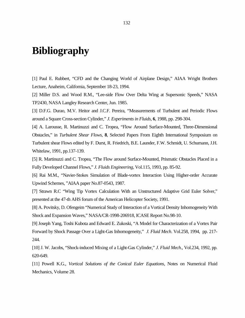
132

Bibliography

[1] Paul E. Rubbert, “CFD and the Changing World of Airplane Design,” AIAA Wright Brothers

Lecture, Anaheim, California, September 18-23, 1994.

[2] Miller D.S. and Wood R.M., “Lee-side Flow Over Delta Wing at Supersonic Speeds,” NASA

TP2430, NASA Langley Research Center, Jun. 1985.

[3] D.F.G. Durao, M.V. Heitor and J.C.F. Pereira, “Measurements of Turbulent and Periodic Flows

around a Square Cross-section Cylinder,” J. Experiments in Fluids, 6, 1988, pp. 298-304.

[4] A. Larousse, R. Martinuzzi and C. Tropea, “Flow Around Surface-Mounted, Three-Dimensional

Obstacles,” in Turbulent Shear Flows, 8, Selected Papers From Eighth International Symposium on

Turbulent shear Flows edited by F. Durst, R. Friedrich, B.E. Launder, F.W. Schmidt, U. Schumann, J.H.

Whitelaw, 1991, pp.137-139.

[5] R. Martinuzzi and C. Tropea, “The Flow around Surface-Mounted, Prismatic Obstacles Placed in a

Fully Developed Channel Flows,” J. Fluids Engineering, Vol.115, 1993, pp. 85-92.

[6] Rai M.M., “Navier-Stokes Simulation of Blade-vortex Interaction Using Higher-order Accurate

Upwind Schemes, ”AIAA paper No.87-0543, 1987.

[7] Strawn R.C “Wing Tip Vortex Calculation With an Unstructured Adaptive Grid Euler Solver,”

presented at the 47-th AHS forum of the American Helicopter Society, 1991.

[8] A. Povitsky, D. Ofengeim “Numerical Study of Interaction of a Vortical Density Inhomogeneity With

Shock and Expansion Waves,” NASA/CR-1998-206918, ICASE Report No.98-10.

[9] Joseph Yang, Toshi Kubota and Edward E. Zukoski, “A Model for Characterization of a Vortex Pair

Forward by Shock Passage Over a Light-Gas Inhomogeneity,” J. Fluid Mech. Vol.258, 1994, pp. 217-

244.

[10] J. W. Jacobs, “Shock-induced Mixing of a Light-Gas Cylinder,” J. Fluid Mech., Vol.234, 1992, pp.

620-649.

[11] Powell K.G., Vortical Solutions of the Conical Euler Equations, Notes on Numerical Fluid

Mechanics, Volume 28.

133

[12] Chi-Wang Shu, “High Order Finite Difference and Finite Volume WENO Schemes and

Discontinuous Galerkin Methods for CFD, ” NASA/CR-2001-210865, ICASE Report No. 2001-11,

May, 2001.

[13] W. Rodi, “Comparison of LES and RANS Calculations of the Flow Around Bluff Bodies,” J. Wind

Eng. and Ind. Aerodyn. 69/71,1997, pp. 55-75.

[14] R. Franke, W. Rodi, “Calculation of Vortex Shedding Past a Square Cylinder with Various

Turbulence Models,” in Turbulent Shear Flows, 8, Selected Papers From Eighth International

Symposium on Turbulent shear Flows edited by F. Durst, R. Friedrich, B.E. Launder, F.W. Schmidt, U.

Schumann, J.H. Whitelaw, 1991, pp. 189-204.

[15] D. Lakehal, W. Rodi, “Calculation of the Flow past a Surface-Mounted Cube with Two-Layer

Turbulence Models,” J. Wind Eng. and Ind. Aerodyn., 67/68, 1997, pp. 65-78.

[16] Kim, J., Moin, P. and Moser, R., “Turbulence Statistics in Fully Developed Channel Flow at Low

Reynolds Number, ” J. Fluid Mech., Vol.177, 1987, pp. 133-166.

[17] Speziale, C.G., “Modeling the Pressure-Gradient-Velocity Correction of Turbulence,” J. Physics of

Fluids, Vol. 28, 1985, pp. 69-71.

[18] Leonard, A., “Vortex Methods for Flow Simulation, ” J. Computational Physics, Vol. 37, 1980, pp.

289-335.

[19] Krasny R., “Vortex Sheet Computation: Roll-up, Wakes, and Seperation,” Lecture in Applied

Mathematics, Vol.28, 1991, pp. 383.

[20] Steinhoff J. and Ramachandran K. “A Vortex Embedding Method for Free-wake Analysis of

Helicopter Rotor Blades in Hover,” Vertica, Vol.13, 1989.

[21] Steinhoff J., Wang C., Underhill D., Mersch T. and Wenren Y., “Computational Vorticity

Confinement: a Non-diffusive Eulerian Method for Vortex Dominated Flows,” Preprint, Tullahoma, TN,

1992.

[22] Steinhoff J. and Mersch T., “Computation of Incompressible Flow Over Delta Wings Using

Vorticity Confinement,” AIAA paper, No.94-0646, 1994.

[23] Steinhoff J., “Vorticity Confinement: a New Technique for Computing Vortex Dominated Flows,”

in Frontiers of Computational Fluid Dynamics (Caughy D. and Hafez M., eds), pp. 235-263, New York:

John Wiley and Sons, 1994.

[24] Steinhoff J., Raviprakash G. and Burley C., “Navier-Stokes Computation of Blade-Vortex

Interactions Using Vorticity Confinement,” In Proc. 33rd Aerospace Science Meeting, Jan.1995.

134

[25] Puskas E., Steinhoff J., Underhill D. and Wenren Y. “Computation of Short Accoustic Pulses,” in

Proceedings, 6th International Symposium on Computational Fluid Dynamics, (Lake Tahoe, NV), 1995.

[26] Steinhoff J., Wenren Y., Wang L., “Efficient Computation of Separating High Reynolds Number

Incompressible Flows Using Vorticity Confinement,” AIAA paper No. 99-3316, 1999.

[27] Wenren Y., Steinhoff J., Wang L., Fan M., Xiao M. “Application of Vorticity Confinement to the

Prediction of the Flow over Complex Bodies,” AIAA paper, No.2000-2621, 2000.

[28] Wenren Y., Fan M., Diets W., Hu, G., Braun C., Steinhoff J., Grossman B., “Efficient Eulerian

Computation of Realistic Rotorcraft Flows Using Vorticity Confinement,” AIAA paper, No.2001-0996,

2001.

[29] Kim, J. et al., “Application of a Fractional-Step Method to Incompressible Navier-Stokes

Equations,” Journal of Computational Physics, Vol. 59, 1985.

[30] Pevchin S., Grossman B. and Steinhoff J., “Capture of Contact Discontinuities and Shock Waves

Using a Discontinuity Confinement Procedure,” AIAA paper 97-0874, Jan. 1997.

[31] Yee K. and Lee D.H. “Euler Calculation For a Hovering Coaxial Rotor Flow Field With New

Boundary Condition,” Paper AE04, 24th European Rotorcraft Forum, Sep.1998.

[32] Jameson A., Schmit W. and Turkel E., “Numerical Solutions of the Euler Equations by Finite

Volume Methods Using Runge-Kutta Time-stepping Scheme,” AIAA paper, No. 81-1359, 1981.

[33] E.Turkel, “Accuracy of Scheme with Nonuniform Meshes for Compressible Fluid Flows,”

Technique Report 85-43, ICASE, 1985.

[34] Turkel E., “Improving the Accuracy of Central Differences Schemes,” in Lecture Notes in Physics,

Vol.323, pp. 586-591, New York: Springer-Verlag, 1988.

[35] Turkel E. and Vatsa V., “Effect of Artificial Viscosity on Three-Dimensional Flow Solutions,” AIAA

Journal, Vol. 32, No. 1, pp. 39-45, 1994.

[36] Caughey D. A., Turkel E., “Effects of Numerical Dissipation on Finite-Volume Solutions of

Compressible Flow Problems,” AIAA paper, No. 88-0621, 1988.

[37] A. Rizzi, “Three-Dimensional Solution to the Euler Equations with One Million Grid Points,” AIAA

Journal, Vol.23, No.13, pp. 1986, Dec.1985.

[38] A. Rizzi and L.E. Eriksson, “Computation of Flow around Wings Based on the Euler Equations,”

Journal of Fluid Mechanics, Vol.148, pp. 45-72, Nov. 1984.

[39] E.M. Murman, A. Rizzi, and K.G. Powell, “High Resolutions of the Euler Equations for Vortex

Flows,” in Progress and Supercomputing in Computational Fluid Dynamics, pp. 93-113, Birkhauser-

Boston, 1985.

135

[40] R.W. Newsome, “A Comparison of Euler and Navier-Stokes Solutions for Supersonic Flow Over a

Conical Delta Wing,” AIAA Paper 85-0111, Jan. 1985.

[41] O.A. Kandil and A. Chuang, “Influence of Numerical Dissipation in Computing Supersonic Vortex-

Dominated Flows,” AIAA paper 86-1073, May 1986.

[42] R.W. Newsome and J.L. Thomas, “Computation of Leading-Edge Vortex Flows,” CP2416, NASA,

1985.

[43] S.R. Chakravarthy and D.K. Ota, “Numerical Issues In Computing Inviscid Supersonic Flow Over

Conical Delta Wings,” AIAA paper 86-0440, Jan. 1986.

[44] F. Marconi, “The Spiral Singularity in the Supersonic Inviscid Flow over a Cone,” AIAA paper 83-

1665, Jul. 1983.

[45] Grossman, B., “A numerical Procedure for the Computation of Supersonic Conical Flows,” Journal

AIAA, Vol. 17, No. 8, pp. 828-837, Aug., 1979.

[46] G. Hu and B. Grossman, “A Numerical Method for Vortex Confinement in Compressible Flow,”

AIAA Paper 2000-0281, Jan. 2000, Reno, NV, USA.

[47] William B. Brower Jr., Tables and Data for Compressible Flow, Hemisphere Publishing

Corporation, 1990.

[48] James J., Quirk and S. Karni, “On the Dynamics of a Shock-bubble Interaction,” J. Fluid Mech.

Vol.318, 1996, pp.139-163.

[49] D.A. Lyn and W. Rodi, “The Flapping Shear Layer by Flow Separation From the Forward Corner

of a Square Cylinder,” J. Fluid Mech., Vol. 267, pp. 353-379, 1994.

[50] D.A. Lyn, S. Einav, W. Rodi and J.H. Park, “A Laser-Doppler Velocimetry Study of Ensemble-

Averaged Characteristics of the Turbulent Near Wake of a Square Cylinder,” J. Fluid Mech., Vol. 304,

pp. 285-319, 1995.

[51] G. Bosh, “Experimentelle und Theoretische Undersuchung der Instationaren Stromung Um

/ylindrische Strukturen,” Dissertation, University of Karlsruhe, 1995.

[52] Leonard, B. P., “ A Stable and Accurate Convection Modeling Procedure Based on Quadratic

Upstream Interpolation,” Comput. Mech. Appl. Mech. Engrg., 19, pp. 59-98, 1973.

[53] Joel H. Ferziger and Milovan Peric, Computational Methods for Fluid Dynamics, Second edition,

Springer, pp. 71-76, 1999.

[54] S. Murakami, A. Mochida, “On Turbulent Vortex Shedding Flows Past 2D Square Cylinder

Predicted by CFD,” J. Wind Eng. and Ind. Aerodyn., 54/55, pp. 91-211, 1995.

136

[55] SangSan Lee, “Unsteady Aerodynamic Force Prediction on a Square Cylinder Using ε−k

Turbulence Models,” J. Wind Eng. and Ind. Aerodyn., 67/68, pp. 79-90, 1997.

[56] P.W. Bearman, E.D. Obasaju, “An Experimental Study of Pressure Fluctuations on Fixed and

Oscillating Square-section Cylinders,” J. Fluid Mech., 119 (1982), pp. 297 –313.

[57] Kishan B. Shah, Joel H. Ferziger, “A Fluid Mechanician’s View of Wind Engineering: Large Eddy

Simulation of Flow Past a Cubic Obstacle,” J. Wind Eng. And Ind. Aerodyn., 67/68, 1997, pp. 211-224.

[58] H. Werner and Wengle, “Large-Eddy Simulation of Turbulent Flow over and Around a Cube in a

Plate Channel,” in Turbulent Shear Flows, 8, Selected Papers From Eighth International Symposium on

Turbulent Shear Flows, edited by F. Durst e R. Friedrich, B.E. Launder, F.W. Schmidt, U. Schumann,

J.H. Whitelaw, 1991, pp.156-168.

[59] S.Z. Yu, A.D. Kowalski, and R.L. Peskin, “An Investigation of Parallel Iterative Algorithms for

CFD, ” in Parallel Computational Fluid Dynamics, edited by Horst, D. Simon, the MIT Press,

Cambridge, Massachusettes, London, England, 1992, pp. 215 - 232.

[60] V. Naik, N. Naik, and M. Nicoules, “Implicit CFD Applications on Message Passing

Multiprocessors Systems,” in Parallel Computational Fluid Dynamics, edited by Horst, D. Simon, the

MIT Press, Cambridge, Massachusettes, London, England, 1992, pp. 97 – 135.

[61] MPI reference: http://www-unix.mcs.anl.gov/mpi/

[62] A. Dadone, G. Hu and B. Grossman, “ Towards a Better Understanding of Vorticity Confinement

methods in Compressible Flow,” AIAA paper 2001-2639, Reno, USA, 2001.

137

Appendix A Characteristic Matrix and Dissipation Models

The characteristic matrix A can be written as follows:

+−−−Φ+−−+−−Φ+−

−−+−Φ+−−−−+Φ+−

=

VnVwnhVvnhVunhVVhnwnVnnvnwnunwnVwnnwnvvnVnnunvnVvnnwnunvnuunVnnVu

nnnn

A

tzyx

zztzyzxz

yyzytyxy

xxzxyxtx

zyxt

ˆˆˆˆˆˆˆˆˆˆˆˆˆˆˆˆˆˆˆˆˆˆˆˆˆˆˆˆ

ˆˆˆˆˆˆˆˆˆˆ0ˆˆˆˆ

ˆ

1010102

0

12112

11212

11122

γγγγγγγγγγγγγγγγ

, (A.1)

where h 0 is the total enthalpy in unit mass, )ˆ,ˆ,ˆ( zyx nnn is the unit normal vector of the grid cell face, and

tn is zero for a fixed grid.

.2,1

),(2

1,/

,ˆˆˆˆ

2

1

2222

00

−=−=

++−=Φ

+=

++=

γγγγ

γρ

wvu

pehwnvnunV zyx

(A.2)

The eigenvalues of matrix A are denoted by 32111 ,,,, λλλλλ and are listed as follows:

138

,ˆˆ

,ˆˆ

,ˆˆ

3

2

1

cVn

cVn

Vn

t

t

t

−+=

++=

+=

λ

λ

λ

(A.3)

where c is speed of sound. Decomposing A , we have

RRA Λ= −1ˆ , (A.4)

where ],,,[ 321,11 λλλλλdiag=Λ ; R is the left eigenvector matrix of A ; 1−R is the right eigenvector

matrix of A , they are given by

−++−−+−+−+−+

=

5554535251

)()()()()()(

1

bbbbbcnwcnwcnnwnwcnwncnvcnvcnvncnvnvncnucnuuncnuncnun

nnn

cR

zzyxzxy

yyzxxzy

xxxyzzy

xzy

KKKKKKK

KKKKKK

KKKKKKK

KKK

ββββββ

ββ

,

(A.5)

+−+−+−−−−−−−

−+−−+−−−+

=−

βγγβγβγββγγβγβγβ

γγγγγγγγγγγγ

111151

111141

111131

111121

111111

1

)()()()()()(

1

cnwcnvcnuacnwcnvcnua

ncnwncnvnunanwncnvncnunancnwnvncnuna

cR

zyx

zyx

xyxzxx

zzxzyz

yxyyzy

)))

)))

))))))

))))))

)))))

,

where 2

1=β and

wnvnunV zyx

++= , (A.6)

139

),(

),(

,)()(

,)()(

,)()(

055

054

1

2

053

1

2

052

1

2

051

hcVbhcVb

cvnwnchnb

cunvnchnb

cwnunchnb

zyx

yxz

xzy

+−=

+=

−+−=

−+−=

−+−=

)

)

)))

)))

)))

ββ

γ

γ

γ

(A.7)

).(

),(

,

,

,

251

241

2231

2221

2211

cVacVa

wcnvcncnna

vcnucncnna

wcnucncnna

yzxx

xyzz

xzyy

−Φ=

+Φ=

−++Φ−=

−++Φ−=

+−+Φ−=

ββ

(A.8)

Now let's turn to the matrix dissipation model D

,

ˆ

ˆ

ˆ

ˆ1

2)(

ˆ

ˆ

ˆ

ˆ1

2)(

0

213

0

112

1

1

−

−

−

−

−+

+

+

+

+

−+=

Λ== −

Vch

ncw

ncv

ncu

l

Vch

ncw

ncv

ncu

ld

RdRdAD

z

y

x

z

y

x

λλλλλ

(A.9)

where

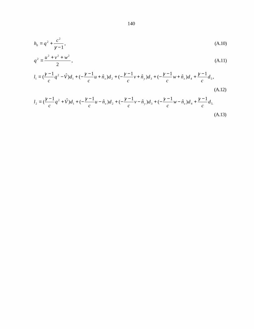
140

1

22

0 −+=γcqh , (A.10)

2

2222 wvuq ++= , (A.11)

,1)ˆ1()ˆ1()ˆ1()ˆ1( 543212

1 dc

dnwc

dnvc

dnuc

dVqc

l zyx−++−−++−−++−−+−−= γγγγγ

(A.12)

.543212

21)ˆ1()ˆ1()ˆ1()ˆ1( d

cdnw

cdnv

cdnu

cdVq

cl zyx

−+−−−+−−−+−−−++−= γγγγγ

(A.13)

141

Appendix B Cross-flow Vorticity and Governing Equations in Conical Coordinates In this Appendix, we will give the details of the derivation of the cross-flow vorticity and governing

equation in conical coordinates

Firstly, we introduce spherical coordinates, φψ ,,r , such that

.cossin,sincos

,cos

ψφψφ

ψ

rzryrx

===

(B.1)

or equivalently

./)(sin

,/tan,

2222

2222

rzyyz

zyxr

+==

++=

ψφ (B.2)

Now we introduce conical coordinates:

./,/

,2222

xzxy

zyxr

==

++=

ηξ (B.3)

142

Now we get the derivatives

,1

,1

,1

1

22

22

22

ηξη

ηξξ

ηξ

++=

++=

++=

r

r

r

z

y

x

(B.4)

,)1(

,)1(1

,)1(

322

322

2

22

322

ηξηξ

ηξξ

ηξ

ηξξ

ξ

ξ

ξ

++

−=

++−

++=

++

−=

rz

rry

rx

(B.5)

.)1(

)1(

,1

,)1(

322

2

22

322

ηξξηξ

ξηηξ

η

η

η

η

++

+=

++

−=

++

−=

rz

ry

rx

(B.6)

Also, we know that the metric terms 2222rrrr zyxh ++= , 2222

ξξξξ zyxh ++= and

2222ηηηη zyxh ++= . After some algebraic work, we get:

143

.1

)1(

,1

)1(

,1

22

21

2

22

21

2

ηξξ

ηξη

η

ξ

+++=

+++=

=

rh

rh

hr

(B.7)

The unit vectors along the conical axes can be expressed in Cartesian coordinates as follows:

).ˆ)1(ˆˆ()1()1(

11ˆ

),ˆˆ)1(ˆ()1()1(

11ˆ

),ˆˆˆ()1(

11ˆ

22/1222/12

22/1222/12

2/122

kjirh

i

kjirh

i

kjirr

hi

rr

ξξηηηξξη

ξηηξηξηξ

ηξηξ

ηη

ξξ

++−−+++

=∂∂=

−++−+++

=∂∂=

++++

=∂∂=

(B.8)

After checking 0ˆˆ =⋅ ξiir and 0ˆˆ =⋅ ηiir , but 0ˆˆ ≠⋅ ηξ ii , we know that conical coordinates are not

orthogonal. The vorticity vector is defined as follows:

kji

wvuzyx

kji

V zyxˆˆˆ

ˆˆˆ

ωωωω ++=

∂∂

∂∂

∂∂=×∇=

, (B.9)

where

.,,

yxz

xzy

zyx

uvwuvw

−=

−=

−=

ωωω

(B.10)

144

According to chain rule

,

,

,

zzzr

rz

yyyr

ry

xxxr

rx

∂∂

∂∂+

∂∂

∂∂+

∂∂

∂∂=

∂∂

∂∂

∂∂+

∂∂

∂∂+

∂∂

∂∂=

∂∂

∂∂

∂∂+

∂∂

∂∂+

∂∂

∂∂=

∂∂

ηη

ξξ

ηη

ξξ

ηη

ξξ

(B.11)

and

,1

,1

,1

1

22

22

22

ηξη

ηξξ

ηξ

++=

∂∂

++=

∂∂

++=

∂∂

zr

yr

xr

(B.12)

,0

,)1(

,)1(

22

22

=∂∂

++=

∂∂

++−=

∂∂

z

ry

rx

ξ

ηξξ

ηξξξ

(B.13)

,)1(

,0

,)1(

22

22

rz

y

rx

ηξη

η

ηξηη

++=

∂∂

=∂∂

++−=

∂∂

(B.14)

145

substituting Eqs. (B.11)-(B.14) into Eq. (B.10), we have:

./)()1(

,/)()1(

,/)()1(

22

22

22

rvvu

rwwu

rvw

z

y

x

ηξξ

ηξη

ηξ

ηξηξω

ηξηξω

ηξω

++++=

++++=

−++=

(B.15)

Finally, we get the three components of vorticity vector in conical Coordinates:

.)1(/)()1(

,)1(/)()1(

,)1(/)(

222/12

222/12

22

ηξωηωξω

ηξωξωηω

ηξηωξωωω

η

ξ

+++−+=

+++−+=

++++=

zx

yx

zxxr

(B.16)

Substituting Eq. (B.15) into rω in Eq. (B.16), we get the expression of cross-flow vorticity in conical

coordinates:

))()((1ηξξηξηηξ ηξηηξξω vvuwwuvw

rr ++−+++−= . (B.17)

We will take the cross-flow vorticity as the vorticity to be used to construct the vorticity confinement.

Now let’s derive the governing equation in conical coordinates. For convenience, the governing equations

in Cartesian coordinates are rewritten here:

SzG

yG

xF

tQ =

∂∂+

∂∂+

∂∂+

∂∂ , (B.18)

where

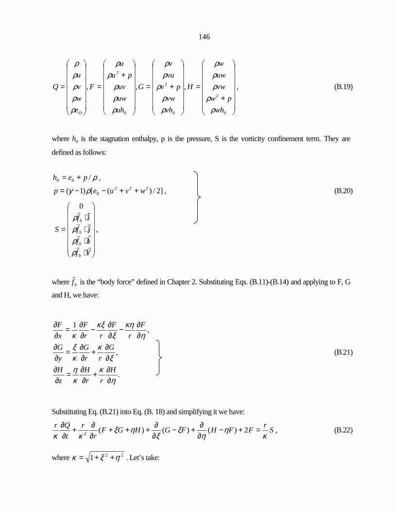
146

+=

+=

+=

=

0

2

0

2

0

2

,,,

whpw

vwuww

H

vhvw

pvvuv

G

uhuwuv

puu

F

ewvu

Q

O ρρρρρ

ρρ

ρρρ

ρρρ

ρρ

ρρρρρ

, (B.19)

where 0h is the stagnation enthalpy, p is the pressure, S is the vorticity confinement term. They are

defined as follows:

ρ/00 peh += ,

]2/)([)1( 2220 wvuep ++−−= ργ , (B.20)

⋅⋅⋅⋅

=

Vfkfjfif

S

b

b

b

b

rr

r

r

r

ρρρρ

ˆˆˆ

0

,

where bf

is the “body force” defined in Chapter 2. Substituting Eqs. (B.11)-(B.14) and applying to F, G

and H, we have:

.

,

,1

ηκ

κη

ξκ

κξ

ηκη

ξκξ

κ

∂∂+

∂∂=

∂∂

∂∂+

∂∂=

∂∂

∂∂−

∂∂−

∂∂=

∂∂

Hrr

HzH

Grr

GyG

Fr

Frr

FxF

(B.21)

Substituting Eq. (B.21) into Eq. (B. 18) and simplifying it we have:

SrFFHFGHGFr

rtQr

κη

ηξ

ξηξ

κκ=+−

∂∂+−

∂∂+++

∂∂+

∂∂ 2)()()(2 , (B.22)

where 221 ηξκ ++= . Let’s take:

147

.~,~

),~

FHH

FGG

HGFF

ηξ

ηξ

−=

−=

++=

(B.23)

Eq. (B.22) can be rewritten as follows:

.2~~~

2 SrFHGrFr

tQr

κηξκκ=+

∂∂+

∂∂+

∂∂+

∂∂ (B.24)

Applying conical assumption 0=∂∂r

to Eq. (B.24), we have:

SrFHGtQr

κηξκ=+

∂∂+

∂∂+

∂∂ 2

~~. (B.25)

Eq. (B.25) is called governing equations in Conical coordinates, where FHGF ,~,~,~ are defined as follows:

,~,~

,~

uwW

uvV

wvuU

ηξ

ηξ

−=

−=

++=

(B.26)

+=

+

−=

+−

=

+++

=

0

2

000

,~

~~

~

~,

~~

~~

~

~,

~~~~

~

~

uhuwuv

puu

F

hWpWw

WvpWu

W

H

hVVw

pVvpVu

V

G

hUpUwpUvpUu

U

F

ρρρ

ρρ

ρρρ

ηρρ

ρρ

ρξρ

ρ

ρηρξρ

ρρ

, (B.27)

where the u, v and w are the three components of velocity vector in Cartesian coordinates.

148

Appendix C Analytical Solution and Initial Condition of a Compressible Moving Vortex with a Uniform Stream

The equation solved in the present study is the unsteady inviscid compressible Euler equations that can be

written as follows:

ρ/pDt

VD −∇=

, (C.1)

where ρ is density, V

is the velocity vector, and p is pressure. We can develop an equation for vorticity

transport by taking the curl of Eq. (C.1) and applying various vector identities. The result is the well-

known vorticity transport equation:

VDtD

)()( ∇⋅=ρω

ρω . (C.2)

This is a general expression that the quantity ρω is transported along material lines for a compressible

isentropic flow.

Next we consider a vortex in a uniform free stream ∞U . Consider an inertial frame with a Cartesian

coordinate system ji ˆ,ˆ and a cylindrical frame fixed to the vortex core θiirˆ,ˆ . We expect the vortex to

move through the flow at a constant speed ∞U or

149

θθ iuiUV ˆˆ += ∞

(C.3)

and that

0=ru . (C.4)

cU

∞∞∞ pU ,,ρ cR

Figure C.1: A compressible vortex moving with a uniform free stream.

We will further model )(ruθ as done by Povitsky and Ofengeim [8] as

≤≤−

<≤=

00

0 ),(~0,/~

)( RrRRr

rR

C

RrRrUru

c

ccc

θ , (C.5)

where

)(

~~

/~

220

0

c

cc

cc

RRRRUC

aUU

−=

= ∞

, (C.6)

0R

150

where ∞a is the speed of sound in the free stream. We can determine the appropriate distribution of p and ρ as follows:

The momentum equation in ),( θr may be written as follows:

θθρ

θρ

θθθθθ

θθ

∂∂−=+

∂∂

+∂∂

+∂∂

∂∂−=−

∂∂

+∂∂

+∂∂

prr

uuur

ur

uut

urp

ruu

ru

ruu

tu

rr

rrr

r

1)(

)(2

. (C.7)

Since 0=ru and )(ruu θθ = we have

0

2

=∂∂

=∂∂

θ

ρ θ

pr

urp

. (C.8)

So )(rpp = and

ru

drdp 2

θρ= . (C.9)

Since the flow is assumed to be isentropic, γρcp = , where c may be evaluated as 1

2

/ −∞

∞∞∞ = γγ

γρρ ap ,

then

drdc

drdp ργργ 1−= , (C.10)

which gives

151

drr

udc2

2 θγ ργρ =− , (C.11)

which, using (C.5), may be integrated to yield

≥

<≤−−−−−−

<≤−−

−

= −−

−−

0

01

12002

0

12

11

22

1

,1

,)])(1(21)ln(2))(1(

21~)1(1[

0,)])(1(2

~)1([

Rr

RrRr

Rr

RRrC

RrRrU

c

cc

cRc

γγ

γγ

γ

γρ

ρ , (C.12)

and

≥

<≤−−−−−−

<≤−−

−

= −−

−−

0

012002

0

12

122

1

,1

,)])(1(21)ln(2))(1(

21~)1(1[1

0,)])(1(2

~)1([1

Rr

RrRr

Rr

RRrC

RrRrU

p c

cc

cRc

γ

γγ

γργ

γγ

γγ

γγ

γ

. (C.13)

Eqs. (C.5), (C.12) and (C.13) are taken as the initial conditions for the vortex moving in a stream problem.

It can be shown that these conditions satisfy compressible continuity, momentum, and energy equations.

Hence theses serve as “exact” solutions to the problem.

152

Vita

The author, Guangchu Hu, was born on April 26, 1963 in Diang Jiang County, Chong Qing Si, P. R.

China. He graduated with a Bachelor’s Degree in Physics in 1984 and a Master’s Degree in Fluid

Mechanical Engineering in 1989 in P. R. China. He began his Ph.D. study at the Aerospace & Ocean

Department of Virginia Tech in the fall of 1997. The next 4 years were spent in pursuit of a Doctorate in

Aerospace Engineering.