IN THE FIELD OF TECHNOLOGYDEGREE PROJECT ENGINEERING PHYSICSAND THE MAIN FIELD OF STUDYCOMPUTER SCIENCE AND ENGINEERING,SECOND CYCLE, 30 CREDITS

, STOCKHOLM SWEDEN 2017

The development and analysis of a computationally efficient data driven suit jacket fit recommendation system

DANIIL BOGDANOV

KTH ROYAL INSTITUTE OF TECHNOLOGYSCHOOL OF COMPUTER SCIENCE AND COMMUNICATION

The development and analysis of a

computationally efficient data driven suit jacket

fit recommendation system

Daniil Bogdanov

daniil@kth.se

Master’s programme in Machine Learning

Supervisor: Alexander Kozlov

Examinator: Mario Romero Vega

December 2017

Abstract

In this master thesis work we design and analyze a data driven suit jacketfit recommendation system which aim to guide shoppers in the process of as-sessing garment fit over the web. The system is divided into two stages. In thefirst stage we analyze labelled customer data, train supervised learning modelsas to be able to predict optimal suit jacket dimensions of unseen shoppers anddetermine appropriate models for each suit jacket dimension. In stage two therecommendation system uses the results from stage one and sorts a garmentcollection from best fit to least fit. The sorted collection is what the fit rec-ommendation system is to return. In this thesis work we propose a particulardesign of stage two that aim to reduce the complexity of the system but at acost of reduced quality of the results. The trade-offs are identified and weighedagainst each other.

The results in stage one show that simple supervised learning models withlinear regression functions suffice when the independent and dependent variablesalign at particular landmarks on the body. If style preferences are also to beincorporated into the supervised learning models, non-linear regression functionsshould be considered as to account for increased complexity. The results instage two show that the complexity of the recommendation system can be madeindependent from the complexity of how fit is assessed. And as technology isenabling for more advanced ways of assessing garment fit, such as 3D bodyscanning techniques, the proposed design of reducing the complexity of therecommendation system enables for highly complex techniques to be utilizedwithout affecting the responsiveness of the system in run-time.

Sammanfattning

I detta masterexamensarbete designar och analyserar vi ett datadrivet rekom-mendationssystem for kavajer med mal att vagleda nat-handlare i deras processi att bedoma passform over internet. Systemet ar uppdelat i tva steg. I det forstasteget analyserar vi markt data och tranar modeller i att lara sig att framstallaprognoser av optimala kavajmatt for shoppare som inte systemet har tidigareexponeras for. I steg tva tar rekommendationssystemet resultatet ifran steg ettoch sorterar plaggkollektionen fran basta till samsta passform. Den sorteradekollektionen ar vad systemet ar tankt att retunera. I detta arbete foreslar vien specifik utformning gallande steg tva med mal att reducera komplexitetenav systemet men till en kostnad i noggrannhet vad det galler resultat. For- ochnackdelar identifieras och vags mot varandra.

Resultatet i steg tva visar att enkla modeller med linjara regressionsfunktio-ner racker nar de obereoende och beroende variabler sammanfaller pa specifikapunkter pa kroppen. Om stil-preferenser ocksa vill inkorpereras i dessa mo-deller bor icke-linjara regressionsfunktioner betraktas for att redogora for denokade komplexitet som medfoljer. Resultaten i steg tva visar att komplexite-ten av rekommendationssystemet kan goras obereoende av komplexiteten forhur passform bedoms. Och da teknologin mojliggor for allt mer avancerade sattatt bedoma passform, sasom 3D-scannings tekniker, kan mer komplexa teknikerutnyttjas utan att paverka responstiden for systemet under kortid.

Contents

1 Introduction 11.1 Background . . . . . . . . . . . . . . . . . . . . . . . . . . . . . . 11.2 Problem formulation . . . . . . . . . . . . . . . . . . . . . . . . . 21.3 Design methodology . . . . . . . . . . . . . . . . . . . . . . . . . 21.4 Research Question . . . . . . . . . . . . . . . . . . . . . . . . . . 41.5 Contributions & Scientific Relevance . . . . . . . . . . . . . . . . 41.6 Delimitation . . . . . . . . . . . . . . . . . . . . . . . . . . . . . . 4

2 Background 62.1 Garment development . . . . . . . . . . . . . . . . . . . . . . . . 62.2 Related work . . . . . . . . . . . . . . . . . . . . . . . . . . . . . 7

2.2.1 Developing a hybrid intelligent model for size recommen-dation . . . . . . . . . . . . . . . . . . . . . . . . . . . . . 7

2.3 Technological advancements . . . . . . . . . . . . . . . . . . . . . 82.3.1 Online fit technologies . . . . . . . . . . . . . . . . . . . . 8

3 Methodology 113.1 Stage one . . . . . . . . . . . . . . . . . . . . . . . . . . . . . . . 11

3.1.1 Handling data . . . . . . . . . . . . . . . . . . . . . . . . 113.1.2 Supervised learning models . . . . . . . . . . . . . . . . . 123.1.3 Linear regression . . . . . . . . . . . . . . . . . . . . . . . 133.1.4 Ridge regression . . . . . . . . . . . . . . . . . . . . . . . 143.1.5 Support vector regression . . . . . . . . . . . . . . . . . . 153.1.6 Performance metrics in stage one . . . . . . . . . . . . . . 18

3.2 Stage two . . . . . . . . . . . . . . . . . . . . . . . . . . . . . . . 183.2.1 K-means . . . . . . . . . . . . . . . . . . . . . . . . . . . . 213.2.2 Performance metrics during stage two . . . . . . . . . . . 22

4 Data collection 274.1 Labelled data for predicting optimal garment dimensions . . . . . 274.2 Unlabelled data for optimizing by clustering . . . . . . . . . . . . 28

5 Results 305.1 Stage one . . . . . . . . . . . . . . . . . . . . . . . . . . . . . . . 30

5.1.1 Data analysis . . . . . . . . . . . . . . . . . . . . . . . . . 305.1.2 Predicting suit jacket dimensions . . . . . . . . . . . . . . 32

5.2 Stage two . . . . . . . . . . . . . . . . . . . . . . . . . . . . . . . 415.2.1 Clustering results . . . . . . . . . . . . . . . . . . . . . . . 415.2.2 Performance results . . . . . . . . . . . . . . . . . . . . . 43

6 Discussion 456.1 Stage one . . . . . . . . . . . . . . . . . . . . . . . . . . . . . . . 45

6.1.1 Supervised learning models . . . . . . . . . . . . . . . . . 456.2 Stage two . . . . . . . . . . . . . . . . . . . . . . . . . . . . . . . 48

6.2.1 Number of clusters . . . . . . . . . . . . . . . . . . . . . . 486.2.2 Modified distance metric . . . . . . . . . . . . . . . . . . . 496.2.3 Trade-offs . . . . . . . . . . . . . . . . . . . . . . . . . . . 496.2.4 Quality of the results . . . . . . . . . . . . . . . . . . . . . 50

7 Conclusion 537.1 Social considerations . . . . . . . . . . . . . . . . . . . . . . . . . 537.2 Stage one . . . . . . . . . . . . . . . . . . . . . . . . . . . . . . . 53

7.2.1 Conclusions . . . . . . . . . . . . . . . . . . . . . . . . . . 547.2.2 Future work . . . . . . . . . . . . . . . . . . . . . . . . . . 54

7.3 Stage two . . . . . . . . . . . . . . . . . . . . . . . . . . . . . . . 557.3.1 Conclusions . . . . . . . . . . . . . . . . . . . . . . . . . . 557.3.2 Future work . . . . . . . . . . . . . . . . . . . . . . . . . . 55

Bibliography 56

Chapter 1

Introduction

1.1 Background

Whether a garment fits or not is critical for consumers in their purchasingdecisions. And while it is possible to try various sizes in physical stores in orderto find the most optimal fit, doing so in digital stores is not. Here shoppers areunable to feel the fabric and texture as well as trying them on before orderingand having them delivered. All though many online garment retailers nowdays complement their products with information and reviews, high qualityphotos and sizing charts to aid with the assessment of fit, they still recognize adisconnect and lack of engagement during the shopping experience between thecustomer and the products [6].

The goal of any sizing chart system is to create sizing charts that definesize groups in such a way as to minimize the number of groups and maximizethe spread in which this sizing system encompasses a given population. Thesesizing charts are created using various methods ranging from trail and error tostatistical methods using computer technology [19, 24, 18]. The problems withsize charts are many, one of which is that manufacturers and brands that createsizing charts look at different populations and sizing variables when developingthese charts. As a consequence, they are seldom coherent and compatible witheach other [8]. In practice this means that despite shoppers know their sizefor a particular garment type, they cannot be sure the same size of anotherbrand will fit equally well. Shopping online thus requires an additional layer ofprecaution as knowledge and information regarding fit is limited. Shoppers maybecome indecisive in their purchasing decision, even discouraged and discontinuebrowsing and as a result, not purchase online. As a consequence, online retailersmay lose potential customers because of the limited engagement and interactionwhile shopping online.

Innovative solutions to the problem of garment fit online are emerging as to-day’s electronic commerce technologies are enabling online retailers to increasetheir level of engagement and interaction with shoppers through out their shop-

1

ping experience [17, 3, 4, 5, 1]. These solutions often come in the form of adigital aid tools or systems that engages with the consumer at different stagesin the shopping process. Thanks to advancements in automated data collectionsystems it is now possible for online retailers to personalize their content aroundthe consumer on a large scale. And in doing so, be able to guide and hopefullyencourage consumers to purchase online.

Another limiting factor to the problem of garment fit online is that thereis still no broadly adopted explicit guidance for assessing fit and no commontheory around the subject [17]. As a consequence, it is difficult to state objec-tively whether a garment fits or not which in turn makes it difficult for onlineretailers to ensure their customers what will fit. Despite much research hasbeen conducted on the topic of anthropometric measurements, garment sizingand fit, little has been documented regarding the technology behind practicalapplications that touch upon these issues [17, 14]. This is mainly due to thefact that they are generally researched and developed through industrial effortsand therefore considered intellectual property.

1.2 Problem formulation

The main problem is that online shoppers are still limited in information re-garding appropriate garment sizes and how they would fit in practice despite ofliving in an information driven society. As a result they may become indecisiveand feel discouraged to continue browsing. We therefore see an opportunity tobuild a system that is designed to give shoppers a better measure on whether thespecific garments they are browsing fit or not. While this measure and guidanceof such system can be achieved in numerous ways, we want to take a more data-rational approach as to be able to personalize content on a global scale. Thepurpose of this thesis work is therefore to design and develop a data driven fitrecommendation system with the aim of aiding online shoppers in their decisionmaking process by providing personalized content and recommend garmentsthat fit.

1.3 Design methodology

The proposed design will focus on the ability to relate customer body data tooptimal garment dimensions as to be able to recommend fitting garments in anefficient way. And because there are yet no broadly adopted explicit guidelinesfor assessing fit, the design will focus less on the assessment and process ofachieving optimal fit. We therefore propose a two stage system that aims to aidcustomers in their assessment of garment fit. The proposed system is illustratedin figure 1.1.

2

Figure 1.1: An overview of the different stages of how data and processes in thedata driven fit recommendation system is to flow. Rounded nodes indicate data,cylindrical nodes indicate databases and rectangular nodes indicate processes.The arrows indicate the flow of data between nodes.

In stage one labelled customer data is used to train supervised learning mod-els as to be able to predict optimal garment dimensions of unseen shoppers. Thelabelled customer data consists of data related to customer’s anthropometric di-mensions and fit preferences together with optimal garment dimensions in theform of historical purchases. Stage two then combines the results from stageone with a fit-evaluator and a collection of garments, that the online shopperwants to sort by fit, and returns a sorted list of garments that is sorted frombest fit to least fit. The approach that would return the most optimal listswould be to evaluate the fit of every garment in the collection and sort themby their corresponding fit score before returning it. This straight forward andoptimal approach will be used as a baseline and will be compared with anotherdesign we propose in this thesis work. This proposed algorithm aim to reducethe computational complexity of the system by clustering data but at a cost ofreturning sub-optimally sorted garment lists (see chapter 3 for more technicaldetails).

3

1.4 Research Question

In the light of the problem of this thesis work and the proposed design methodol-ogy described above, the investigation of this work in stage one will focus on thedegree predictability and in stage two; how the results changes by the proposeddesign of this thesis work. In stage one, it will be of importance to considerhow the data is to be pre-processed and represented and selecting appropriatesupervised learning models. In stage two, it will be of importance to consideran appropriate clustering algorithm and how the results of the proposed designare to be measured and compared to the baseline approach which returns opti-mal results. The research question for this thesis work may therefore be scopeddown to encapsulate the questions that the research of this work may answer.We therefore formulate the explicit research question as follows:

What supervised learning model, in combination with which representation ofdata, is suitable for a data driven garment fit recommendation system as to beable to predict optimal garment dimensions?

And as we propose a novel design in this thesis work, we are inclined to analyzehow this affects the results of the system. We therefore hope that the workof this thesis will be able to address issues regarding the implications of suchdesign in terms of computational complexity, speed and accuracy of the results.

The design of this system is intended to be driven by data. The availabledata of this thesis work will therefore be the essential factor in answering theresearch question, but also constitute the validity of this work (see chapter 4 forspecifications of the available data).

1.5 Contributions & Scientific Relevance

The work of this thesis will be another attempt in creating innovative web toolsfor online garment retailers aimed to aid consumers in their online shoppingexperience. To the best of my knowledge, there is very little research in theliterature on intelligent size recommendation systems in garment industry asthey predominately stem from industrial efforts [22, 17]. The work of this thesisis therefore a novel attempt in developing a data driven garment fit recom-mendation system described above. The outcome of this thesis work aim tocontribute to the scientific body of knowledge that concerns with data drivenapplications related to garment fit and hope to function as a reference for anyfurther improvements in future work.

1.6 Delimitation

Whilst the findings of this thesis work regarding the recommendation system isintended to function of any garment type, the work of this thesis will be limitedto developing a system that only considers suit jackets. The reason for this is

4

that the available customer data only include suit jacket dimensions. This willenable a deeper, rather than a broad, development and analysis process. Also,suit jackets are one of the most common apparel garments in men’s fashion andis the reason for why this particular garment type was chosen. The idea is thatthe findings of this thesis work can in future work be extrapolated to othergarment types. However, this will require separate data analysis as differentanthropometric dimensions may have to be considered. As a consequence of thislimitation, the design choices will be kept general and avoid designing aroundthe specifics that relate only to suit jackets.

A significant limitation that affects both the methodology and findings ofthis work is the limited size of available labelled customer data. A Swedishretailer specializing in men’s fashion have contributed with a sample set undershort notice in order to make this work possible. And as such data is regardedcommercially sensitive, the raw data will not be included in this report.

5

Chapter 2

Background

In this section we present the related background to this thesis work. In sec-tion 2.1 We give a broad overview of the various components in the process ofgarment development and production. In section 2.2 we give a brief overview ofacademic work related to garment fit recommendation systems. Lastly, in sec-tion 2.3 we present related recommendation systems which stem from industrialefforts.

2.1 Garment development

Garments are a natural and obvious necessity for us humans. Wearing garmentsthat fit is of great importance, especially in the realm of fashion. Therefore italso matters to all involved parties in the garment production process. Theseparties include product development teams, garment manufacturers and fashionretailers who all have different drivers and influence the process in different ways.In every step in the process of development, manufacturing and sales of garmentsthere are important factors that affect other parts of the chain that has to beconsidered. Product developers and designers want to encompass as a broadspectrum of body shapes as possible while at the same time keeping the numberof design patterns low. Garment manufacturers want to keep the process simpleand production cost low while being able to meet the specifications from thegarment designers. Garment retailers wants to be able to offer something to all oftheir customers while keeping reasonable stock sizes. The garment productionprocess is complex and versatile and difficult to influence as a whole. It istherefore important for all involved parties to know their capabilities, limitationsand goals and understand between which parties along the chain they would fitthe best and thus benefit the most.

Garment fit is a complex area for several reasons, one of which is that thereis yet no broadly adopted explicit guidance for assessing fit [17]. Academics,industries and consumers have divergent definitions of fit and engage with gar-ments at different stages which makes it difficult for the research area to stay

6

concise. Another reason is that there is no clear theory which can or is used toexplain the assessment of fit and how this can be achieved. As a consequence, itis difficult to compare results that stem from divergent definitions which makesthe research area fragmented.

2.2 Related work

The research regarding the problem of specifying the right garment size forconsumers is limited. While there exists numerous papers regarding the devel-opment of data driven sizing chart systems, there are very few papers directlyrelated to the topic of this project work [17]. Work related to data drivenrecommendation systems are increasing in popularity as current technology isenabling machine learning techniques to scale efficiently and generate value tocompanies. These systems may help to recommend other products whenever acustomer have bought or browsed a certain product, or recommending musicthat the system believe the listener would like based on similar attributes ofthese songs. These recommendation systems differ a lot from garment fit rec-ommendation systems. These popular recommendation systems generally tryto find abstract representations of some objects and learn how to discriminatebetween these abstract representations given some input in the form of pref-erences or behavior. Garment fit recommendation systems on the other handrepresent objects (may it be body shapes and sizes or garments) using theirmeasurements and the recommendation schema is based on heuristics related tothe assessment of fit. Because of this difference in approaches, we omit present-ing recommendation systems in general and focus instead on recommendationsystems that are directly related to garment fit and sizing. But because suchsystems emerge mostly through industrial efforts, offering little or no insightsto how they function, the related work of this project will be limited. The onlydirectly related paper found in the literature is by J Shahrabi et al. which isdiscussed below.

2.2.1 Developing a hybrid intelligent model for size rec-ommendation

J Shahrabi et al. in [22] develops a hybrid intelligent classification model as asize recommendation expert system. The development is done in three stagesand is based on data clustering and uses a probabilistic neural network (PNN)which achieve an 87.2 percent accuracy rate. They build this model using suitsize data of Iranian males.

In the first stage they use agglomerate hierarchical clustering (AHC) todetermine the number of clusters in their data which was determined to fiveclusters. K-means algorithm is used to segment the heterogeneous populationinto five clusters as AHC proposed. To evaluate the clustering algorithm, theyaggregated the loss of fit by considering only three dimensions (determined byconsulting with domain experts) which are chest circumference, waist circum-

7

ference and hip circumference. In the second stage, the resulting clusters in thefirst stage represent a new sizing chart which is used as a reference to train aPNN using Dynamic Decay Adjustment (DDA) algorithm. In the third and laststage they evaluate the accuracy of the trained model using a portion of the datathat was withheld during training. They state that the accuracy they achievedon the test set was promising and would in practice help the salesperson guidetheir consumers in choosing the right size.

2.3 Technological advancements

The advancements in computer technology and the increased accessibility of theinternet in the past decade has enabled online fashion retailers to operate ona truly global scale. It has opened up new ways and channels to expose onesproducts and reach new consumers around the world. This new way of engagingwith consumers is of a digital form which differ from physical shopping experi-ences and places numerous restrictions and poses new challenges. Products thatconsumers expect to feel and try as a part of the shopping experience beforedeciding on purchasing them, such as garments, are difficult to simulate overthe web.

However, with this advancement in computer technology, practices stemmingfrom machine learning (and interdisciplinary fields such as computer vision andnatural language processing to name a few) are enabling the development ofincreased digital engagement and personalized content on a global scale. Thesefields offer techniques of solving various problems in the textile industries atvarious levels of complexity and innovation. In this thesis work we will utilizewell known machine learning techniques and practices. We therefore omit topresent any work related to machine learning and instead present the techniquesused in the next chapter.

2.3.1 Online fit technologies

It has been identified that the level of engagement through out the online shop-ping experience is a key factor to success [13]. This is why industries haveadopted their engagement strategies and started to focus more on how to uti-lize the technological advancements described above to develop aiding onlinefunctionality.

All though there is yet no broadly adopted explicit guidance for assessinggarment fit and no common ground theory around the subject which can beused to explain the assessment of fit and how it is achieved, there are emergingsolutions from various companies [17, 3, 4, 5, 1]. Most solutions are in the formof online tools that provide the opportunity for consumers to engage in the fitprocess and provide means to capture the experience of fit. But because thesesolutions stem from the industry and not academic research, these solutionsare commercially sensitive as they build upon sensitive customer data and areviewed as intellectual property. As a result, the inner workings of these tools

8

are not presented but instead an overview on how they are intended to functionis given below.

Fits Me

Fits me provides consumers with either size prediction or a virtual fitting roomexperience for a selection of retailers. Their size prediction tool is based ona limited number of personal consumer data such as the consumer’s height,weight, age and bra size for women together with a fit preference in the formof selection of a body shape. The technology then combines garment dataincluding silhouette and stretch properties and shopper data to determine whichsize garment will fit the consumer [3]. As most shoppers do not fit perfectlyinto a standardized size, their system helps decide which compromises to makein order to achieve the best fit possible. They offer size prediction dependingon brand and limited functionality for certain brands for key pieces [17].

True Fit

True Fit is a data driven personalization platform for footwear and apparelretailers. They use rich connected data and machine learning methods to providepersonalized fit ratings and size recommendations to shoppers [4]. Their systemencompass product data from over 1000 brands with fit and style attributesabout each item, deriving on average 181 attributes per item and maps therelationship between product attributes and consumer preferences. This systemis not only based on measurements but also on the recommendation on historicalperformances and inferences [2].

Virtusize

Virtusize is a garment-to-garment online comparison tool that enables shoppersto compare garments with either previous purchases or with garments theyalready own. Comparison between garments are made with two to four keymeasurements and presented to the shopper by showing overlaying silhouettesof the garments that are being compared. Their view is that garment comparisonis the only way to clearly and objectively showcase size and fit in contrast toother popular online tools who are based on body measurements [5].

Mesher

Mesher is a smart phone application which uses the camera on a smartphoneto calculate one’s body dimensions and provides personalized clothing recom-mendation based on these calculated measurements [1]. It requires only threepictures to be taken in order to calculate one’s body dimensions; one picture ofthe shopper from the front, one from the side and one of the background withoutthe shopper in the picture. the application then calculates the shopper’s bodydimensions using computer vision technology and projective geometry. This ap-proach works around the classical measurement tape and helps shoppers relate

9

their body dimensions to garment products via their product feed. One advan-tage of this approach is that you are able to make a body profile on your own incontrast to using the classical measurement tape that requires assistance fromanother person in order to achieve accurate measurements.

10

Chapter 3

Methodology

In this chapter we present the models and techniques used through out the workof this thesis and described them in detail. Section 3.1 describes the supervisedlearning models and related techniques that can be used in predicting optimalsuit jacket dimensions. Section 3.1.6 describes the metrics used in evaluatingthese supervised learning models. Section 3.2 describes the cluster algorithmsthat is part of the proposed approach in optimizing the computational load ofthe system. And lastly, section 3.2.2 describes the methods and metrics used inevaluating the optimized system to the baseline system.

3.1 Stage one

The purpose of constructing supervised models in stage one is to be able to usethese models to infer optimal garment dimensions for shoppers with no previouspurchase history. This will enable us to assess garment fit by comparing optimalgarment dimensions to other garment dimensions directly instead of defining fiton a body-to-garment basis. The goal of this stage is thus to build and trainsuch models while avoiding overfitting as the available data is limited.

3.1.1 Handling data

This section describes how the data in the supervised learning task at hand willbe utilized. Familiarizing and analyzing the data can help to uncover existingrelationships between variables and which models would be more or less suitable.Furthermore, in order to successfully solve the task with limited data, it is wiseto look into as how one may utilize the available data to the fullest.

Correlation matrix

A correlation matrix describes the pair-wise correlation between the variablesin the data. A correlation between two variables, a and b, with mean values

11

µa and µb and standard deviations σa and σb may be specified by a correlationcoefficient defined as such

ρa,b =E((a− µa)(b− µb))

σaσb(3.1)

where E is the expected value operator. Then, by computing the correlationcoefficient for each pair of variables in the data, the result can be presented asa symmetric matrix called the correlation matrix. The matrix is symmetric asρa,b = ρb,a, which is why it suffices to only present the correlation matrix aseither a lower or upper triangular matrix.

The correlation matrix can indicate a predictive relationship between vari-ables which can further be exploited. Note however that it only indicates acorrelation and is not sufficient to infer a causal relationship. Other statisticalmeasures must be deployed in order to make such inferences.

Leave-P-Out cross validation

Leave-P-Out Cross Validation (LPOCV) is a model validation technique thatis used to study how well a model would generalize to independent data setswithout any additional data set at one’s disposal. Having a total of N datapoints, the technique removes P samples from the data set and creates

(NP

)pairs of complementary subsets; a training set and a test set. The idea is tothen train and evaluate the predictability of each trained predictor for each pairof training and test set. This will generate

(NP

)metric values where the mean

may indicates the model’s generalization capabilities. This technique is suitablewhen N is small as it helps to avoid overfitting which is likely to happen in suchcases.

3.1.2 Supervised learning models

The aim of a supervised learning task is in a general sense to construct a map-ping between two domains of data. The problem consists in finding a suitabletransformation function from labelled training data to some target domain andthe goal of this function is to make accurate predictions of new, unseen data [15].Each data point contains of two pieces of data, one from each domain, wherethe first piece of data is regarded as the available input to the task at hand andthe second piece of data is what to be inferred through the first domain.

Supervised learning tasks are categorized depending on the nature of datain the domain we want to predict. If the predicted data is of discrete nature,the problem is categorized as a classification problem. If the predicted data isreal and continuous, then the problem is categorized as a regression problem.In this thesis we will tackle a regression problem as suit jacket dimensions canspan over a continuous range of values. In this setting, we want to construct afunction that infers a mapping between two different sets of variables. In ourcase the first set is the set of variables describing body related data and theother set is the set of variables describing suit jacket dimensions.

12

Motivation of choice

In order to attempt to solve the supervised learning task at hand, suitablealgorithms for the nature of the problem and considering the conditions haveto first be determined. For garments that require a high degree of fit, suchas fashion wear, consistent body landmarks that relate to available garmentdimensions are important to identify [11]. This means that the closer and morerelevant the anthropometric dimensions are to any of the suit jacket dimensions,the more accurate one can make prediction models.

It is also desirable for the mapping between these two sets of variables tohave a continuous shape as to reflect the non-discontinuous variation in bothanthropocentric data and garment dimensions. This motivates us to disregardsupervised learning models that produce discontinuous predictors such as re-gression trees, ensembles of regression trees and K-nearest neighbors.

Furthermore, given our small data size, supervised learning models such asartificial neural networks that often require a lot of training data in order toperform well will be a poor choice of design. Despite its popularity and predic-tion capabilities for even non-linear problems, considering simpler model will bea smarter choice of design since a small data size is not suitable with models ofhigh flexibility and complexity. Designing with simplicity in mind and aligningthe methodology to the nature of the problem, balancing the capabilities withone’s limitations, is the preferred practice to success.

3.1.3 Linear regression

Linear regression is a method for modelling the relationship between a set of in-put variables and a set of continuous target variables. The relationships aremodeled using linear functions and the model consists of parameters calledweights that are estimated from the training data. If, for example, we wantto use p independent variables, x = (x1, . . . , xp), to model one target variable,y, this model can be represented as such

y(x) = w0 + w1 · x1 + · · ·+ wp · xp = w0 +

p∑i=1

wi · xi ≈ y (3.2)

where y is the linear function model approximating y and w0, . . . , wp are theweights. In our case x is a input vector that represents the anthropometricdimensions of an individual. The target variable, y, represents a particular suitjacket dimension which we want to predict from x. This method can easilybe generalized to incorporate multiple output values resulting in multivariatelinear regression.

To make the notation more compact, one can redefine x as x ≡ (1, x1, . . . , xp)and define a weight vector w ≡ (w0, . . . , wp)

T which gives the compact form

y(x) = 〈x,w〉 (3.3)

13

where 〈·, ·〉 is the dot product operation. If we then consider N samples, stackingeach sample’s input vector on top of each other and the corresponding targetvalues on top of each other, forming a matrix sometimes called the design matrixX = [x0,x1, xN ]T with N rows and p + 1 columns and a target vector Y =(y0, . . . , yN )T , we can construct any linear model by minimizing the residual sumof squares between the true target variables in the dataset, Y , and the predictedtarget variables Y = Xw by linear approximation [21]. This approach is calledOrdinary Least Squares (OLS) and mathematically it solves the problem byminimizing the expression

minw

N∑i=1

||xi ·w − yi||22 = minw||Xw − Y ||22 = min

w||Y − Y ||22. (3.4)

However, this technique rely upon the fact that the input vectors in X arelinearly independent. When these vectors are linear combinations of each otherthe design matrix have an approximate linear dependence and multicollinearitymay arise. This means the weights of the model can become large in theirvalues and highly sensitive to random noise and errors in the observed target,producing a large variance and undesirable behavior.

3.1.4 Ridge regression

To address the problem of multicollinearity which may occur when using theordinary least square technique we can impose a penalty term related to the sizeof the model weights as a mean to control the large variances that may occur.This is a regularization technique sometimes referred to as ridge regression [16].Each regularization term is categorized by their norm and multiple terms withdifferent norms may be present at the same time. The optimal choice of normis problem specific.

This technique, in its simplest form, can be expressed with an additionalterm in the objective expression (3.4) as such

minw||Xw − Y ||22 + α||w||q. (3.5)

where q ∈ N determines the norm and α ∈ R > 0 the amount of shrinkage.these parameters are regarded as hyperparameters as they relate more to theproperties of the models rather then to what is being modelled. The mostcommon norms are q = 1 or q = 2 but may be used in combination with eachother.

The choice of q and α should not be inferred from the training data similarto how the model weights are determined. Instead, one should use a third dataset, a validation set, in order to tune these parameters appropriately as not tobias the trained model around the training data too much. This requires anadditional partitioning of the data which in some cases is unfeasible as the data

14

is already limited. One therefore have to balance bias and variance that existin the problem appropriately.

Regularization techniques may also be used to guide the process in choosingrelevant input variables. When q = 2, the technique will dampen the weightvalues of all input features. But when q = 1, the technique may completely sup-press some weights as to keep the number of relevant features low [16]. Choosingthe optimal value of q depends on the problem at hand and is something oftendetermined by trail and error.

3.1.5 Support vector regression

Support Vector Regression (SVR) is another supervised learning algorithm usedfor regression problems. SVR is regarded to be efficient in high dimensionalspace and still effective in cases where the number of dimensions is greater thanthe number of samples. The model produced by SVR depends only on a subsetof training points as the cost function for building the model ignores trainingpoints close to the model prediction. SVR produce continuous predictors witha high degree of complexity which makes them suitable for our task at hand.

The goal of SVR is to construct a function y(x) that has at most ε deviationfrom the observed target yi for all the training data, and at the same time is asflat as possible [23]. In the simple case of a linear function y, taking the form

y(x) = 〈x,w〉 (3.6)

where w = (w0, . . . , wp)T , x = (1, x1, . . . , xp). Flatness in this case of (3.6)

means to find a small w. One way to achieve this is to minimize the norm of w,i.e. ||w||22. Thus we can write this problem as a convex optimization problem:

min1

2||w||22

s.t

yi − 〈xi,w〉 ≤ ε〈xi,w〉 − yi. ≤ ε

(3.7)

(3.8)

This formulation assumes there exists a function y that approximates alltraining points (xi, yi) with ε precision. However, this may not always be thecase. We therefore introduce slack variables ξi, ξ

∗i to handle infeasible con-

straints of the optimization problem (3.7). We then reformulate our problem assuch

15

min1

2||w||22 + C

N∑i=1

(ξi + ξ∗i )

s.t

yi − 〈xi,w〉 ≤ ε+ ξi

〈xi,w〉 − yi. ≤ ε+ ξ∗i

ξi, ξ∗i ≥ 0

(3.9)

where the slack-strength constant C > 0 determines the trade-off between theflatness of y and the amount of deviation larger than ε in such cases.

One can formulate this optimization problem in its dual form and are in mostcases easier to solve [9]. Here we use a standard dualization method utilizingLagrange multipliers. We combine our objective together with our constraintsto form the Lagrange function which takes the form

L :=1

2||w||22 + C

N∑i=1

(ξi + ξ∗i )−N∑i=1

(ηiξi + η∗i ξ∗i )−

∑Ni=1 αi(ε+ ξi − yi + 〈xi,w〉)−

∑Ni=1 α

∗i (ε+ ξ∗i − yi − 〈xi,w〉)

(3.10)where ηi, η

∗i , αi, α

∗i ≥ 0 are the Lagrange multipliers.

The partial derivatives of L with respect to the primal variables, w0, . . . , wp,ξ1, . . . , ξN and ξ∗1 , . . . , ξ

∗N , have to vanish which corresponds to

∂w0L =

N∑i=1

(α∗i − αi) = 0 (3.11)

∂wL = w −N∑i=1

(αi − α∗i )xi = 0 (3.12)

∂ξiL = C − αi − ηi = 0 (3.13)

∂ξ∗i L = C − α∗i − η∗i = 0. (3.14)

Substituting the above results of the derivations into (3.9) yields the dual opti-mization problem

max

− 12

∑Ni,j=1(αi − α∗i )(αj − α∗j )〈xi,xj〉

−ε∑Ni=1(αi + α∗i ) +

∑Ni=1 yi(αi − α∗i )

s.t∑Ni=1(αi − α∗i ) = 0 and αi, α

∗i ∈ [0, C].

(3.15)Note that we can rewrite equation (3.12) as follows

16

w =

N∑i=1

(αi − α∗i )xi (3.16)

which states that our weights can be described solely by a linear combinationof the training samples xi. This gives our predictor function the new form

y(x) =

N∑i=1

(αi − α∗i )〈xi,x〉. (3.17)

This rewriting is called Support Vector expansion and free us from computing wexplicitly. Instead we evaluate y(x) in terms of dot products between the data.As a consequence, this allows us to generalize to implicit nonlinear mappings byapplying the kernel trick [20]. We introduce a kernel function and restate ouroptimization problem as such

max

− 12

∑Ni,j=1(αi − α∗i )(αj − α∗j )k(xi,xj)

−ε∑Ni=1(αi + α∗i ) +

∑Ni=1 yi(αi − α∗i )

s.t

N∑i=1

(αi − α∗i ) = 0 and αi, α∗i ∈ [0, C]

(3.18)

where k(xi,xj) is the kernel function. We may also rewrite our predictor func-tion (3.17) using the kernel function as such

y(x) =

N∑i=1

(αi − α∗i )k(xi,x). (3.19)

This gives the freedom in constructing regression functions of different shapesas the kernel function can take on many forms e.g. polynomial kernel

k(x,x′) = (γ〈x,x′〉+ r)d (3.20)

of degree d, or a sigmoid kernel

k(x,x′) = tanh(γ〈x,x′〉+ r) (3.21)

where γ, r and d are hyperparameters.In this nonlinear setting, the optimization problem corresponds to finding

the flattest predictor function in this non-linear feature space, not in input spaceas in the linear case mentioned earlier.

17

3.1.6 Performance metrics in stage one

To evaluate how well a supervised learning model describes the underlying re-lationship, several metrics may be considered. In this work we will evaluatethe trained model’s prediction capabilities by consider the coefficient of deter-mination. The coefficient of determination can be computed for any supervisedlearning model which makes it suitable for comparing different models. Also,this metric is scale invariant which makes it a suitable metric for comparingmodels that require inputs to be scaled to models that do not require this.

Coefficient of determination

The coefficient of determination is a metric that indicates the proportion of thevariance in the target variables that is predictable from the input variables tothe variance in the target variables that exist in the problem at hand. Thecoefficient of determination is denoted R2 and is defined as

R2 = 1−∑

(y − y)2∑(y − y)2

= 1− Model error

Intrinsic error(3.22)

where y is the inferred predictor and y is the mean value of the target data. R2

has an upper bound of 1 but no lower bound. The numerator in the fractionis the sum of squared error predictions (sometimes denoted SSR for Sum ofSquared Residuals) and is where a model influences this metric. The denomi-nator in the fraction is the total sum of squares (sometimes denoted TSS) andis a quantity that indicates the variance in the target variables of the problem.As a result, R2 indicates how much of the total variance can be explained usingour trained predictor.

3.2 Stage two

The purpose of the proposed design in stage two of the recommendation systemis to make it computationally efficient as to be able to handle cases where thegarment collection may be large and the response time of the system needs tobe small. Even short delays can disrupt the consumer’s shopping experiencewhich is why the possibility of making this system responsive in practice is ofinterest to online fashion retailers. The proposed design alleviates the needfor having to use the fit-evaluator in run-time. This enables for an arbitrarilycomplex fit-evaluator as it is only used offline during the construction or furtherimprovement of the system. The goal of this proposed approach is to reducethe computational complexity of the system while retaining similar degree ofquality in the resulting output as the baseline system. In order to achieve this,a novel approach is proposed below.

The proposed design in making the system computationally efficient involvessolving an unsupervised learning task. More specifically, a clustering task. The

18

purpose of a clustering task in a general sense is to find groups of objects suchthat the objects within a group are similar to one another and different to objectsbelonging to other groups. In our case, the purpose of clustering garment data isto find centers of groups of garments with similar dimensions, also called clustercenters or centroids. These centroids could then act as representatives for aregion of garments with similar dimensions. The system can then constructgarment index lists offline by pre-computing fit scores using the fit-evaluatorand sorting the collection in a descending order with respect to fit. This is donefor each centroid. Then, when a customer wants to sort the collection by fitin run-time, the centroid closest to this customer’s optimal garment dimensionswill act as a ’best’ approximation and that centroid’s already sorted garmentlist will be returned, not having to make any fit-related computations of thiscustomer directly during run-time other than finding the closest centroid. Thedifferent systems are visually illustrated in figure 3.1.

19

Figure 3.1: Illustration of how the two different systems in stage two are in-tended to operate. Elliptical nodes indicate data structures, cylindrical nodesindicate databases and rectangular nodes indicate functions. Solid arrows in-dicate the flow of data between different nodes while dashed arrows indicatenode dependencies during the construction of different nodes. Note that in theoptimized system there is no fit evaluator. Instead, a database is constructedand used to fetch garment index lists of the closest centroid.

20

The main differences between the baseline and the optimized system is thatthe proposed design have replaced the fit evaluator with a database containingsorted lists of garment indices for every centroid. As a result, whilst the baselineapproach requires the use of the fit-evaluator to sort the collection in run-time,the proposed design is not dependent on the fit-evaluator in run-time.

Motivation of choice

In order to attempt to make this system computationally efficient using theapproach described above, a suitable clustering algorithm for the nature of theproblem needs to be determined. Since the results of the clustering procedureis not the final results of this task but rather a middle step, the choice ofwhat clustering algorithm to use is not crucial but nonetheless important to besuitable for the nature of the data of this task.

The data consists of standardized sized suit jacket dimensions which isanisotropic in their nature (see section 4.2 for more details). Whilst Gaus-sian mixture models are suitable for clustering such data, the objective of thistask is not to group the data into appropriate clusters considering the skewnessof the data but rather generate centroids that act as representatives of a smallisotropic region in the garment space. This motivates us to use a rather simplebut popular and intuitive clustering algorithm such as K-means despite the databeing anisotropic.

3.2.1 K-means

K-means is a clustering algorithm which objective is to minimize the averagesquared distance between points in the same cluster. It is a well known NP-hardproblem to solve exact but nonetheless a popular clustering algorithm used ina wide range of scientific and industrial applications [10].

In essence, given a set, X , of N data points, x ∈ Rl, where l is the number ofdimensions defining a garment, the goal is to choose k centroids as to minimize

φ =∑x∈X

minc∈C||x− c||2 (3.23)

which represents the total squared distance between each point x and its clos-est centroid c. This is sometimes refereed to as the inertia of the clusteringprocedure. Since its formulation, many attempts in solving this problem hasbeen proposed and various greedy algorithms have been developed as an ap-proximate solution [7]. One popular greedy algorithm which generates solutionsto this problem is Lloyd’s algorithm.

The k-means algorithm is simple to understand, fast computationally wisebut guarantees no global solution. The procedure is as follows:

1. Arbitrarily choose an initial k centroids C = {c1, c2, . . . , ck}

2. For each i ∈ {1, . . . , k}, set the cluster Ci to be the set of points in X thatare closer to ci than they are to cj for all i 6= j.

21

3. for each i ∈ {1, . . . , k}, set ci to be the center of mass of all points in Ci.

4. Repeat steps 2 and 3 until C no longer changes.

However, the initial values in the first step of this algorithm influences theperformance. Hence there has been some research and development in choosingthese initial centroids in a more cleaver way.

K-means++

One algorithm which currently tries to address the problem of poor initial cen-troid selections in k-means is k-means++. It differs from the traditional k-meansalgorithm only in the first step when choosing values of the initial centroids andcan be seen as an improvement to the initialization of the original k-means al-gorithm. Here, the initialization process utilizes a distance function D(x) whichcomputes the distance between x and the nearest centroid at that time. Theadditional steps can be summarized as such

1. Choose one center, c1, chosen uniformly at random from X

2. For each point in X compute D(x)2.

3. Choose a new center, ci, choosing x ∈ X with probability D(x)2∑x∈X D(x)2

4. Repeat step 2 and 3 until we have considered all k centroids.

5. Proceed to step 2 of the standard k-means algorithm.

With this approach, all though we accumulate a small additional overhead com-putations to find better initial centroid position, we gain both accuracy andspeed by choosing k-means++ over ordinary k-means clustering algorithm [7].

3.2.2 Performance metrics during stage two

To analyze how the proposed design affects the output of the system, we haveto understand how the results differ from the baseline approach. And as theresult of such recommendation system is in the form of a sorted list, containinggarments from most optimal fit to least optimal fit, the results of the differentapproaches will differ in the order in which these garments are sorted as eachsystem will have slightly different sorting objectives. The sorting in turn isbased on how we define and assess garment fit. We therefore need to addresshow fit is to be assessed and define appropriate metrics that may be used toevaluate the results of the proposed design.

22

Assessment of fit

Different garment dimensions impact the appearance of fit differently. For ex-ample, if the sleeve length of a suit jacket is off by 1 cm from one’s optimallength, this garment is a better fit than a garment that is instead off with 1 cmby shoulder-width as shoulder-width is obviously a more sensitive dimensionthan sleeve-length to compromise with. This is why weighing the different di-mensions accordingly would be of importance when considering the assessmentof fit. But for this study, no data containing information of how much eachdimension affects the overall fit in relation to other dimensions were available.Instead, we make use of the output in stage one which were predicted optimalgarment dimensions and compare each dimension pair-wise and directly to othergarment dimensions as such

f(j g, ∗g) =

l∑i=1

(j gi − ∗gi)2 (3.24)

where j g is shopper j’s predicted optimal garment dimensions, ∗g is some gar-ment we are evaluating and l is the number of dimensions defining a garment.In this way we may compare each dimension directly and let discrepancies inany direction from the predicted optimal garment dimensions contribute to thisunfitness score. Also, this approach of assessing garment fit is on a garment-to-garment basis which circumvents the troubles in assessing fit between twodifferent domains. Furthermore, defining a unfitness function in contrast to afitness function will not impinge on the generality of this analysis as the inverseof either one may automatically define the other one.

Spearman’s footrule distance

The Spearman’s footrule distance is a metric used to measure the dissimilarityof two lists containing the same elements but in different orders. This is exactlywhat the different design approaches in stage two produces which makes thismetric suitable for understanding how the results may differ. In technical terms,this metric measures the aggregated absolute distance between the rankings ofevery element in the two lists. As a consequence, this metric is invariant as itdoes not depend on the identify of the elements, only their rank [12].

If πj and σj are two ranking lists of length N , produced by different recom-mendation systems, where j denotes the jth shopper, the Spearman’s footruledistance may be defined as

Dj = D(πj , σj) =

N∑i=1

|πj(i)− σj(i)| (3.25)

where N is the total number of elements in the lists. But since the baselinedesign returns the most optimal results, we set πj(i) = i to reflect the fact that

23

the baseline system outputs the most optimal garment lists as it uses customerj’s predicted optimal garment dimensions as its sorting objective directly. Wetherefore rewrite the function above to be independent of the first list as such

D(πj , σj) = D(σj) =

N∑i=1

|i− σj(i)| (3.26)

However, this metric fail to take into account important aspects such aselement relevance and positional information. Various contributions has beenmade in order to generalize and improve this metric [25]. We extend this metricto our needs and incorporate positional information as well as element similarity.

Positional information

The Spearman’s footrule distance metric can be improved by considering thefact that elements in the top of the ranked lists may affect the metric morethan elements in the end of the ranked list if they were to be found at differentpositions in the lists πj and σj . Different factors can be incorporated intoeach term in the summation in equation (3.26) depending on the preference ofimportance between ranks. In our case, we want garments with good fit i.e. thatappear in the top of the ranked list to be of more importance than garmentsthat have a lesser fit score associated to them.

Different positional weighing distributions were considered as shown in figure3.2.

24

Figure 3.2: Various positional weight distributions of a list with arbitrary num-ber of elements.

By favoring a distribution which give more importance to elements in thebeginning of the ranked list while maintaining a continuous shape, we decidedfor this study to use a exponential decay as our positional weighing distribution.The metric can now be rewritten as such

D(σj) =

N∑i=1

|i− σj(i)| · e−a(i−1)b

(3.27)

where a, b are scaling parameters that limits the exponential factor between (0,1]within the rank range [1,N ].

Element similarity

The Spearman’s footrule distance metric can further be improved by consideringthe fact that when two garments, with very similar dimensions, are swappedthe metric should result in a small change whereas swapping two garments withradically different dimensions should have a large impact.

To incorporate such behavior into our metric we will make use of the unfit-ness function defined above. Let us first define τj = {gi}Ni=1 to be the rankedgarment collection of length N of customer j of the baseline system where gi

25

is the ith garment in that list and τj to be the garment collection that is per-muted according to σ as a result of this optimization approach for customerj. Then, by considering the absolute difference between the unfitness score ofgarment τj(i) = gi and τj(i) we capture how similar the swapped garment is tothe original garment of rank i.

We now extend the metric to incorporate element similarity as such

D(σj , τj , τj) =

N∑i=1

|i− σj(i)| · e−a(i−1)b

· |f(gj , τj(i))− f(gj , τj(i))| (3.28)

where gj is the predicted optimal garment dimensions of customer j.Note that if f(xj , τj(i)) = f(xj , τj(i)) for a particular rank i and customer

j and some garment vector xj , the swapped garments have the exact sameunfitness score and their contribution to the metric measuring the similarity oftwo lists will not be affected despite two elements have been swapped.

Relating fit to performance metrics of the results

Spearman’s footrule distance and the modified version described above will mea-sure how dissimilar two lists are to each other, which in turn may describe howdissimilar the results from two different systems are to each other. But to un-derstand how the results differ in terms of fit score and not garment rankings,we turn our attention to how such a metric may be constructed.

One possibility is to sum the unfitness score of all garments in the returnedlist and compare this value to the output of the proposed design. However, thesum will equal each other as the difference between these systems are only theordering of the garments in the returned list. We therefore suggest to weigh theelements in the list with their rank using the same distribution as the positionalweight distribution used in the modified Spearman’s footrule distance describedabove. By incorporating the positional information into this metric, the metric isable to differentiate between systems of different outputs while still only relatingthis metric to fit scores. The weighing will be done for both systems and thisperformance metric will be normalized with the value of the baseline system toacquire relative metrics as the baseline design’s output is already regarded asthe most optimal one.

26

Chapter 4

Data collection

In this chapter, we present the different data sets that is to be used duringthe work of this thesis. As there are two stages to the system, each stage willutilize different data sets. Section 4.1 describes the labelled data used in the firststage of the system which is to construct models that predict optimal garmentdimensions. Section 4.2 describes the unlabelled data used in optimizing thecomputational load of the system.

4.1 Labelled data for predicting optimal garmentdimensions

Each data point in the labelled data set consists of 12 input variables and 5target variables. The input variables correspond to

• 3 body distance measurements,

• 6 body circumference measurements,

• 1 body property and

• 2 body preferences.

There are 7 available data points in this data set and their attributes are sum-marized in table 4.1.

The 9 body dimensions are shoulder-width, shoulder circumference, chest cir-cumference, waist circumference, hip circumference, shoulder to tumble (StT)distance, biceps circumference, neck circumference and height. Let these bodymeasurements be denoted as b1, . . . , b9 respectively. Furthermore these at-tributes all have numerical values. The single body property corresponded to theindividual’s weight which is also a numerical value. Let the weight be denotedb10. Let b denote all these body dimensions.

The 2 preference attributes were the individuals length and ease preference.These correspond to categorical values between (both included) 1 to 5 and

27

represent how they generally prefer their suits in terms of suit length and easearound the torso. For length preference, the value 1 represents preferring a shortsuit jacket and the value 5 represents preferring a tall suit jacket in general. Forthe ease preference, the value 1 corresponds to preferring a tight suit and value5 corresponds to preferring a lose suit jacket around the torso. Let these twopreferences be denoted p1 and p2 respectively and as p = (p1, p2) collectively.

The target variables correspond to the common suit jacket dimensions (seefigure 4.1 for visual description) and are shoulder-width, half-back, half-waist(closed), back-length and inner sleeve-length. Let these be denoted g1, . . . , g5respectively and as g = (g1, . . . , g5) collectively.

Variable Measurement type Notation Value type Data type

Shoulder Distance b1 Numerical Input

Shoulder Circumference b2 Numerical Input

Chest Circumference b3 Numerical Input

Waist Circumference b4 Numerical Input

Hip Circumference b5 Numerical Input

Shoulder to tumble Distance b6 Numerical Input

Biceps Circumference b7 Numerical Input

Neck Circumference b8 Numerical Input

Length Distance b9 Numerical Input

Weight Property b10 Numerical Input

Length Preference p1 Categorical Input

Ease Preference p2 Categorical Input

Shoulder-width Distance g1 Numerical target

Half-back Distance g2 Numerical target

Half-waist (closed) Distance g3 Numerical target

Back-length Distance g4 Numerical target

Inner sleeve-length Distance g5 Numerical target

Table 4.1: Input and target variables for each data point in the labelled dataset used in stage one of the system for constructing supervised learning models.

4.2 Unlabelled data for optimizing by clustering

Each data point in the unlabelled data set represents a standardized suit jacketand contains 6 common dimensions associated with the suit jacket as well asits try-on size. The garment dimensions are shoulder-width, half-back, half-waist (closed), half-waist (open), back-length and inner sleeve-length. Thesedimensions are illustrated in figure 4.1. There are 72 available data points in

28

this data set. But because the labelled data set (see table 4.1) is missing half-waist (open), this dimension will be excluded in the design of this system.

Figure 4.1: Common dimensions for standardized ready-to-wear suit jackets.Each letter and corresponding arrow indicate the dimensions. These are A)shoulder-width, B) half-back, C) half-waist (closed), D) half-waist (open), E)back-length, F) inner sleeve-length.

The data set contain suit jackets from various fit categories such as Reg-ular, Slim, Superslim, Regular stout, Slim stout, Slim tall and Superslim tall.The data set is already filtered to not contain suit jackets of identical garmentdimensions.

Table 4.2 shows one data point from every fit category including their try-on size. Note that because this data set consist of ready-to-wear suit jacketsthat have been designed in a standardized way, the dimensions between try-one sizes are scaled incrementally. As a consequence, the data is anisotropic asdimensions are scaled with the try-one size.

Fit Try-on size g1 g2 g3 g4 g5

Regular 42 43.4 20.6 44.0 75.0 41.9

Superslim 44 41.4 20.2 44.0 71.0 44.4

Slim 48 44.5 22.4 48.0 75.0 43.4

Silm tall 82 41.4 20.6 41.0 75.0 44.0

Slim stout 22 42.4 21.2 46.0 70.0 39.9

Table 4.2: Data set with entries of varying Fit category.

29

Chapter 5

Results

In this chapter, we present the results of the two parts of this thesis work.First, in section 5.1.1, we identify correlating variables in the labelled data set.Then, in section 5.1.2, we present the results of the different supervised learningmodels and compare them to one another. Lastly, in section 5.2.1, we presentthe clustering and performance results of the proposed design choice in stagetwo.

5.1 Stage one

5.1.1 Data analysis

A correlation matrix was constructed to find correlations between different vari-ables in the data. A correlation would suggest some kind of relationship betweentwo variables as they will exhibit a tendency to behave similarly within a specificsetting which is what we are looking for. However, this analysis cannot concludea definitive causation relationship which is why various model representationswill be built and tested using variables that correlate with each other.

30

Figure 5.1: Lower triangular correlation matrix over the available input andtarget variables of the labelled data set.

It is of interest to inspect the 5 last rows in figure 5.1. This is where wecan identify correlations between the target variables and the input variables.The correlation matrix in figure 5.1 indicate that g1, the suit jacket shoulder-width, strongly correlates with b1, the body shoulder-width, as expected sincethey share the same landmarks. The two strongest correlating variables of eachtarget variable is summarized separately in table 5.1 and table 5.2.

31

Target variable Input variable Correlation

g1 (suit shoulder-width) b1 (body shoulder-width) 0.916

g2 (half-back) b4 (waist circumference) 0.859

g3 (half-waist (closed)) b4 (waist circumference) 0.935

g4 (back-length) b6 (shoulder to thumble) 0.908

g5 (sleeve-length) b6 (shoulder to thumble) 0.901

Table 5.1: Details of the strongest correlating input variable to the each indi-vidual target variable.

Target variable Input variable Correlation corr(first, second)

g1 (suit shoulder-width) b7 (biceps) 0.600 0.645

g2 (half-back) b10 (weight) 0.850 0.758

g3 (half-waist (closed)) b10 (weight) 0.766 0.758

g4 (back-length) b10 (weight) 0.858 0.769

g5 (sleeve-length) b9 (height) 0.898 0.963

Table 5.2: Details of the second strongest correlating input variable to eachindividual target variable. The last column describe the correlation betweenthe strongest and the second strongest correlating input variable for each targetvariable.

The top correlating input variables for each target variable will be usedto construct different predictors, first using only the most correlating inputvariable, then only the second strongest correlating variable, then combiningthem both and finally the optimal feature representation for each target variablefound by trial and error. Other combinations of input variables will also betested to see whether the prediction capabilities can be increased for each targetvariable. These results are presented in the next section.

5.1.2 Predicting suit jacket dimensions

The supervised learning task is divided into 5 regression problems, one for eachsuit jacket dimension. And for each suit jacket dimension we perform a leave-3-out cross validation which generates

(73

)= 35 different regression functions

for each model. The main focus of this analysis is to determine an appropriatesupervised learning model and suitable input variables for each target variableby considering the aggregated R2 scores. The mean R2 score, the mean R2

score of only the positive instances and the ratio of instances with positive R2

were noted for each cross validation run.

32

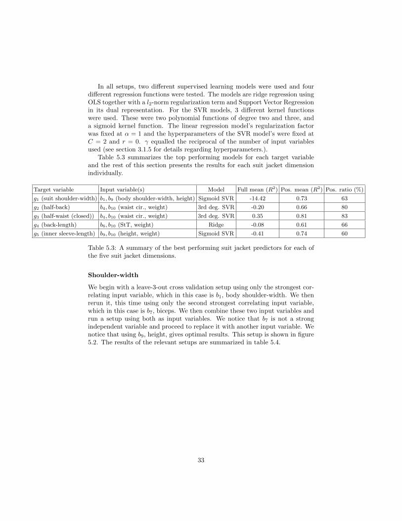
In all setups, two different supervised learning models were used and fourdifferent regression functions were tested. The models are ridge regression usingOLS together with a l2-norm regularization term and Support Vector Regressionin its dual representation. For the SVR models, 3 different kernel functionswere used. These were two polynomial functions of degree two and three, anda sigmoid kernel function. The linear regression model’s regularization factorwas fixed at α = 1 and the hyperparameters of the SVR model’s were fixed atC = 2 and r = 0. γ equalled the reciprocal of the number of input variablesused (see section 3.1.5 for details regarding hyperparameters.).

Table 5.3 summarizes the top performing models for each target variableand the rest of this section presents the results for each suit jacket dimensionindividually.

Target variable Input variable(s) Model Full mean (R2) Pos. mean (R2) Pos. ratio (%)

g1 (suit shoulder-width) b1, b9 (body shoulder-width, height) Sigmoid SVR -14.42 0.73 63

g2 (half-back) b4, b10 (waist cir., weight) 3rd deg. SVR -0.20 0.66 80

g3 (half-waist (closed)) b4, b10 (waist cir., weight) 3rd deg. SVR 0.35 0.81 83

g4 (back-length) b6, b10 (StT, weight) Ridge -0.08 0.61 66

g5 (inner sleeve-length) b9, b10 (height, weight) Sigmoid SVR -0.41 0.74 60

Table 5.3: A summary of the best performing suit jacket predictors for each ofthe five suit jacket dimensions.

Shoulder-width

We begin with a leave-3-out cross validation setup using only the strongest cor-relating input variable, which in this case is b1, body shoulder-width. We thenrerun it, this time using only the second strongest correlating input variable,which in this case is b7, biceps. We then combine these two input variables andrun a setup using both as input variables. We notice that b7 is not a strongindependent variable and proceed to replace it with another input variable. Wenotice that using b9, height, gives optimal results. This setup is shown in figure5.2. The results of the relevant setups are summarized in table 5.4.

33

Figure 5.2: R2 scores of a leave-3-out cross validation setup of different predic-tors. Every predictor used b1 and b9 as input variables and suit jacket shoulder-width dimension as their target variable.

full R2 mean pos. R2 mean pos. ratio (%)

Ridge 2nd 3rd Sigmoid Ridge 2nd 3rd Sigmoid Ridge 2nd 3rd Sigmoid

Input var.

b1 -26.97 -39.23 -19.51 -30.45 0.65 0.59 0.52 0.65 0.57 0.46 0.63 0.57

b7 -96.72 -200.61 -457.76 -66.97 0.32 0.03 0.16 0.20 0.40 0.06 0.11 0.37

b1, b7 -37.46 -64.2 -19.58 -36.37 0.56 0.46 0.40 0.63 0.57 0.43 0.40 0.66

b1, b9 -11.93 -96.53 -11.6 -14.42 0.68 0.33 0.60 0.73 0.63 0.43 0.54 0.63

Table 5.4: Aggregated metrics of different models predicting optimal suit jacketshoulder-width dimension using various input variables. The values in the col-umn category ’full R2 mean’ corresponds to the mean score of all iterations,’pos. R2 mean’ corresponds to the mean score of instances with only positiveR2 score.

34

Half-back

We begin with running a leave-3-out cross validation setup using only thestrongest correlating input variable, which in this case is b4, waist circumfer-ence. We then rerun it, this time using only the second strongest correlatinginput variable, which in this case is b10, weight. We then combine these twoinput variables and run a setup using both as input variables. Through someadditional experimental setups we conclude that using both b4 and b10 achievesthe best results. This setup is shown in figure 5.3 and the results of the relevantsetups are summarized in table 5.5.

Figure 5.3: R2 scores of a leave-3-out cross validation setup of different predic-tors. Every predictor used b4 and b10 as input variables and suit jacket half-backdimension as their target variable.

35

full R2 mean pos. R2 mean pos. ratio (%)

Ridge 2nd 3rd Sigmoid Ridge 2nd 3rd Sigmoid Ridge 2nd 3rd Sigmoid

Input var.

b4 -2.18 -5.72 -0.80 -13.03 0.44 . 0.42 0.26 40 0 49 26

b10 -12.1 -5.8 -12.27 -33.33 0.36 0.19 0.38 0.26 34 11 51 31

b4, b10 -7.25 -5.04 -0.20 -21.85 0.37 . 0.66 0.23 57 11 80 29

Table 5.5: Aggregated metrics of different models predicting optimal half-backdimension using various input variables. The values in the column category’full R2 mean’ corresponds to the mean score of all iterations, ’pos. R2 mean’corresponds to the mean score of instances with only positive R2 score.

Half-waist (closed)

We begin with running a leave-3-out cross validation setup using only thestrongest correlating input variable, which in this case is b4, waist circumfer-ence. We then rerun it, this time using only the second strongest correlatinginput variable, which in this case is b10, weight. We then combine these twoinput variables and run a setup using both as input variables. Through someadditional experimental setups we conclude that using both b4 and b10 achievesthe best score. This setup is shown in figure 5.4 and the results of the relevantsetups are summarized in table 5.6.

36

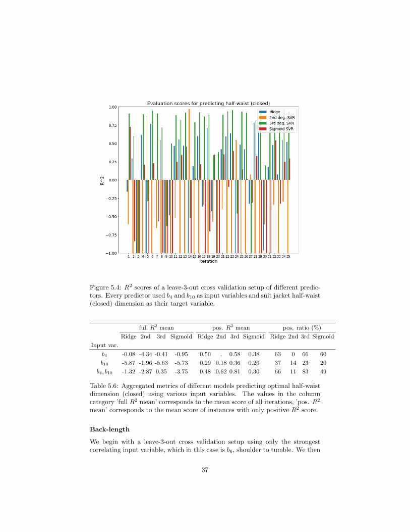
Figure 5.4: R2 scores of a leave-3-out cross validation setup of different predic-tors. Every predictor used b4 and b10 as input variables and suit jacket half-waist(closed) dimension as their target variable.

full R2 mean pos. R2 mean pos. ratio (%)

Ridge 2nd 3rd Sigmoid Ridge 2nd 3rd Sigmoid Ridge 2nd 3rd Sigmoid

Input var.

b4 -0.08 -4.34 -0.41 -0.95 0.50 . 0.58 0.38 63 0 66 60

b10 -5.87 -1.96 -5.63 -5.73 0.29 0.18 0.36 0.26 37 14 23 20

b4, b10 -1.32 -2.87 0.35 -3.75 0.48 0.62 0.81 0.30 66 11 83 49

Table 5.6: Aggregated metrics of different models predicting optimal half-waistdimension (closed) using various input variables. The values in the columncategory ’full R2 mean’ corresponds to the mean score of all iterations, ’pos. R2

mean’ corresponds to the mean score of instances with only positive R2 score.

Back-length

We begin with a leave-3-out cross validation setup using only the strongestcorrelating input variable, which in this case is b6, shoulder to tumble. We then

37

rerun it, this time using only the second strongest correlating input variable,which in this case is b10, weight. We then combine these two input variables andrun a setup using both as input variables. We also run a setup where we useb9, the height, as the only input variable. But as this input variable does notcorrelate with the target variable as much as the previous tried input variables,b9 as input variable does not yield better results. Through some additionalexperimental setups we find that using both b6 and b10 achieves the best score.This setup is shown in figure 5.5 and the results of the relevant setups aresummarized in table 5.7.

Figure 5.5: R2 scores of a leave-3-out cross validation setup of different pre-dictors. Every predictor used b6 and b10 as input variables and suit jacketback-length dimension as their target variable.

38

full R2 mean pos. R2 mean pos. ratio (%)

Ridge 2nd 3rd Sigmoid Ridge 2nd 3rd Sigmoid Ridge 2nd 3rd Sigmoid

Input var.

b6 -0.42 -2.88 -1.38 -1.32 0.57 . 0.34 0.35 54 0 43 40

b10 -0.79 -3.30 -0.10 -0.68 0.44 0.19 0.59 0.39 57 11 66 46

b9 -1.69 -0.93 -3.35 -1.72 0.42 0.34 0.35 0.30 49 34 34 46

b6, b10 -0.08 -4.73 -1.05 0.16 0.61 . 0.42 0.52 66 0 54 74

b9, b10 -1.4 -1.98 -0.46 -1.12 0.46 0.17 0.36 0.34 40 9 57 34

Table 5.7: Aggregated metrics of different models predicting optimal back-length dimension using various input variables. The values in the column cat-egory ’full R2 mean’ corresponds to the mean score of all iterations, ’pos. R2

mean’ corresponds to the mean score of instances with only positive R2 score.

Sleeve-length

We begin with running a leave-3-out cross validation setup using only thestrongest correlating input variable, which in this case is b6, Shoulder to tumble.We then rerun it, this time using only the second strongest correlating inputvariable, which in this case is b9, height. We then combine these two inputvariables and run a setup using both as input variables. We also run a setupwhere we use b10, weight, as the only input variable. But as this input variabledoes not correlate with the target variable as much as the previous tried inputvariables, b10 as input variable does not yield better results. All though throughsome additional experimental setups we find that predictors using b9 and b10,height and weight, as input variables yield the best results. This setup is shownin figure 5.6 and the results of the relevant setups are summarized in table 5.8.

39

Figure 5.6: R2 scores of a leave-3-out cross validation setup of different pre-dictors. Every predictor used b9 and b10 as input variables and suit jacketsleeve-length dimension as their target variable.

full R2 mean pos. R2 mean pos. ratio (%)

Ridge 2nd 3rd Sigmoid Ridge 2nd 3rd Sigmoid Ridge 2nd 3rd Sigmoid

Input var.

b6 -0.39 -4.84 -1.76 -1.51 0.51 . 0.25 0.41 57 0 23 51

b9 -1.12 -4.29 -0.83 -2.59 0.66 0.20 0.31 0.47 57 11 43 63

b10 -3.10 -4.33 -0.86 -4.93 0.42 0.26 0.41 0.40 54 06 40 29

b6, b9 -0.80 -4.41 -0.78 -1.82 0.60 . 0.28 0.43 60 0 29 57

b9, b10 -0.83 -5.58 -0.22 -0.41 0.68 0.23 0.32 0.74 60 17 40 60

Table 5.8: Aggregated metrics of different models predicting optimal innersleeve-length dimension using various input variables. The values in the col-umn category ’full R2 mean’ corresponds to the mean score of all iterations,’pos. R2 mean’ corresponds to the mean score of instances with only positiveR2 score.

40

5.2 Stage two

5.2.1 Clustering results

During the clustering task, the total number of clusters was varied from 1 to 72(total number of data points in the unlabelled data set) and for each prespecifiednumber of clusters the algorithm described in section 3.2.1 was performed 50times. Each run was stopped after 500 iterations or if the inertia got less thana prespecified threshold of 0.0001. Figure 5.7 shows how the inertia convergesdown to 0 as the number of clusters approach the number of garments in thecollection, which is the expected value the algorithm should converge to.

Figure 5.7: The red scale shows the objective function of k-means++ clusteringprocedure and the blue scale shows the mean offset distance between a subjectand its closest centroid.

Since the clustering is done in 5 dimensions the results are hard to visualize.Instead we plot each pair of dimensions to each other together with the clustercenters. This is shown in figure 5.8.

41

Figure 5.8: Each plot shows a projection in two dimensions of the clusteringresults. The blue crosses represent a garment, the orange crosses representcluster centers, the red circles represent subjects and the red dashed lines aredrawn between subjects and their closest centroid in five dimensional space.

42

5.2.2 Performance results

Finally we show how the modified Spearman’s footrule distance and the accuracyvaries with the total number of clusters.

Figure 5.9: The graph shows how the modified Spearman’s footrule distancevaries with the total number of clusters. The distance is computed using all thesubjects and each bar shows the mean value in each iteration.

43

Figure 5.10: The blue graph shows how the normalized weighted unfitness scoreof the optimized system varies with the total number of clusters. The blue graphconverges to the value 1.006.

This is shown in figure 5.9 and figure 5.10 respectively. The clustering algo-rithm is guaranteed to converge which these figures confirm. But the values towhich the respective metrics converge is of interest to compare to other similarsystems but preferably with different configurations and models.

44

Chapter 6

Discussion

In this chapter we discuss findings in the results of this thesis work. Section6.1 discusses both the general performance of the trained supervised learningmodels and also interesting findings for some of the predictors in stage one.Section 6.2 discusses findings, comparisons between metrics, trade-offs and thequality of the results of the proposed design.

6.1 Stage one

6.1.1 Supervised learning models

Considering the most optimal predictors, both ridge regression and SVR per-formed well on different regression problems and were suitable supervised re-gression models for the nature of this task. However, because the learningalgorithm of SVR does not penalize on data points that are within ε deviationfrom their true target value, the algorithm does not strive to further improveits predictability once within this range. As a consequence, and in combinationwith having all hyperparameters of these models fixed during the training pro-cess of all regression problems, the trained models only achieve sub-optimal R2

scores. But as the data of this work is limited, tuning hyperparameters wouldmost likely result in overfitted predictors. Furthermore, the goal of this task wasnot to achieve the highest possible R2 score but rather determine and confirmappropriate supervised learning models and corresponding input variables.

Shoulder-width

During the leave-3-out cross validation setup one can notice in figure 5.2 that adistinct set of iterations (iteration 6-25) where all the predictors performed withpredominately positive results while in other regions all predictors performedpoorly (iteration 1-5 and 26-35). On close inspection one can understand thatthis is due to the fact that this data can roughly be clustered into two groups.And if the data points in the test set are predominately contained within only

45

one of these clusters, the predictors will seem to perform poorly. Figure 6.1shows two different iterations with very different evaluation results.

Figure 6.1: Shows two particular iterations of the leave-3-out cross validationsetup for ridge regression models predicting optimal suit jacket shoulder-widthdimensions using b1 as the only input variable. The left graph shows iteration6 which achieved a R2 score of 0.95 and the right graph shows iteration 26(see figure 5.2 for all iterations) which achieved a R2 score of -6.82. Note thedifferences in errors due to the positioning of the test data points.

The active choice in choosing to perform a leave-P-out cross validation (P =3) setup revealed that the choice of split of this small data set into a trainingset and a test set have a big impact on the evaluation results. Here we avoiddeeming any model as poorly performing as we evaluate the models in a morebroader view rather than in only one single partitioning of the data. This isalways possible but seldom feasible as it scales drastically with the total numberof data points. In this case it is feasible as the data size is very small.

46

Half-back & half-waist (closed)

The best performing predictor for predicting suit jacket half-back and half-waist (closed) dimensions respectively used the same input variables which werethe two top strongest correlating body-related properties to respective targetvariable. As both target variables correlate with similar input variables, onewould suspect that the target variables correlate with each other, which indeedis the case. The correlation coefficient for half-back and half-waist (closed) isas strong as corr(g2, g3) = 0.965. As a direct consequence, similar models forpredicting these target variables should perform similarly, which indeed is thecase. Figure 6.2 shows various isocurves of the best performing predictor forrespective target variable. Both these predictors have a third degree polynomialkernel function.

Figure 6.2: Shows iteration 6 of the leave-3-out cross validation setup for pre-dictors with different target variables but same kernel function. Both predictorsuse b4 and b10 as input variables. The isocurves correspond to different valuesof the second input variable b10, body weight.

Both predictors achieved higher R2 scores compared to predictors with only

47

one input variable. However, both predictors in figure 6.2 intersect with oneanother, which is not a desirable behavior and not suitable in practice. Thisis a consequence of searching for an optimal predictor function in a non-linearfeature space and not in the data space directly. To avoid this as best as possible,more data needs to be provided in order to guide the learning algorithm inseparating such cases from each other.

Back-length

The input variables that yielded the highest R2 score when predicting the back-length dimension was the combined variables b6 and b10, shoulder to tumble andweight. It is surprising that b6, shoulder to tumble, yielded better predictionsthan when using b9, height, which has more relevant landmarks. But as b6,in this limited data set, correlate better with g4, back-length, this result isreasonable.

Inner sleeve-length

The input variables that yielded the highest R2 score when predicting the innersleeve-length dimension was the combined use of b9 and b10, height and weight.These two input variables relate to the body’s vertical and horizontal scale andmay be the reason to why it yielded highestR2 scores. Furthermore, using heightyielded better predictions than when using b6, shoulder to tumble, as inputvariable despite it correlated stronger with the target variable. This shows thatonly choosing input variables solely on their correlation to the target variablemay not always yield the best results.

6.2 Stage two

6.2.1 Number of clusters

The k-means algorithm requires that you pre-specify the number of clustersbefore it can proceed. The analysis was therefore run at various numbers ofclusters, ranging from one cluster up to and including 72 clusters which is theamount of garments in the collection of this analysis. To determine an appro-priate cluster number one can consider several metrics. Both the mean offsetshown in figure 5.7 and the modified Spearman’s footrule distance shown in fig-ure 5.9 behave similarly and could be an appropriate indicator for determiningthe number of clusters. A low metric value is desired, and in either case theconsistently lowest values can be found when the number of clusters are roughlybetween 40-50. However, these metrics only indicate how much the optimizedsystem differs from the base line and not to what extent the final results areaffected.

48

6.2.2 Modified distance metric

Comparing the original version of Spearman’s footrule distance with the modi-fied version we can observe that the modified version, in contrast to the originalversion, exhibit a shape similar to the accuracy, or unfitness scoring, of the op-timized system. These differences and similarities are shown in figure 6.3. Notethe flatness of the original version in contrast to the modified version. Bothdistances indicate that the solution converges after around 50 clusters but themodified version also incorporates the information in the contents of the listswhich makes this distance metric a better candidate.

Figure 6.3: The graphs shows how the different Spearman’s footrule distancestogether with the non-normalized unfitness scoring of the optimized systemvaries with the total number of clusters. Each metric is computed using all thesubjects and the graphs shows the mean value of each iteration.

6.2.3 Trade-offs

The purpose of optimizing the system is to make it computationally efficientin practice by circumventing the fit evaluator in run-time, but at a cost ofreturning a sub-optimally sorted garment collection. The optimized system does

49

not consider how the customer’s predicted optimal garment dimensions relateto the garment collection directly, instead it utilizes a database with pre-sortedgarment indices for every centroid and returns a sorted garment collection w.r.t.the closest centroid’s fit preferences. One can therefore state that the optimizedsystem utilizes data storage to reduce computations but at a cost of returningsub-optimally sorted garment lists.

The amount of storage needed in order for such a system to function de-pends on the number of clusters and the size of the relevant garment collection.The information to be stored is a sorting scheme for every centroid. And inits smallest form, this would correspond to a list of integers specifying whichgarment is to be placed at that entry of the list. In practice, the minimumamount of storage will vary depending on what digital platform is used and howthe system is implemented in relation to the rest architecture.

The reduced computational complexity depends on the computational com-plexity of how fit is computed and the size of the relevant garment collection.In an optimized system, the system neither has to compute fit scores for everygarment in the collection or sort the results w.r.t. unfitness. Instead the op-timized system only needs to find the closest centroid and return the garmentcollection according to its sorting scheme. Thus, the computational complexityof an optimized system in the second stage, in contrast to a baseline system,only scale with the number of clusters and not with the size of the garment col-lection. This approach is therefore suitable when the collection of items neededto be sorted is large and a small infringement on the accuracy of the results isaffordable.

6.2.4 Quality of the results

The normalized weighted unfitness score gives an indication on how the systemperforms in comparison to the baseline system. Figure 5.10 shows that the opti-mized system’s relative accuracy decreased with a percentage of 0.6 units, whichmay sound affordable in many cases. But what are the practical implicationsand how does this affect the quality of the system? By considering the ratioof garments that retained their position in the optimized system, we see thatonly about a fifth of the garments retain their rank as the number of clustersapproach the number of garments in the collection. This is shown in figure 6.4.

50

Figure 6.4: The graph shows the mean ratio of how many garments retain theirrank between the optimized and non-optimized system.

Whilst the ratio between non-displaced garments and displaced garments isas low as 0.25, it raises an interest in examining the distribution of displacedgarments. If we then pick a cluster number that corresponds to an instancewhere the system almost converged but at the same time keeping the clusternumber low, we settle with k = 45. During this iteration, we can observe infigure 6.5 that the majority of far-displaced garments are garments scatteredaround the middle of the lists. Furthermore, figure 6.6 shows more exactlywhere the rank-retained garments are located using a binary heatmap plot. Itshows that the first garment of each subject’s returned list retained rank andthat the majority of rank-retained garments spread around the end of each list.Retaining ranks in the end of the list is of lesser relevance as they correspondto garments that fit the least. Nonetheless, the system of the proposed designmanaged retain the rank of the first garment which may be regarded as the mostimportant garment to retain as its fits the best and is therefore most relevantfor the shopper.

51

Figure 6.5: The heatmap represents the original Spearman’s footrule distance,indicating how far each garment has been displaced in the optimized system. Adark color indicates a low displacement distance while a bright color indicatesa high displacement distance.

Figure 6.6: The heatmap indicates if a particular garment in the optimizedsystem has been displaced or not. Yellow indicates a garment with retainedrank while purple indicates the garment has been displaced.

52

Chapter 7

Conclusion

In the last chapter we present the conclusions of the different stages of the systemseparately. Section 7.2 presents the conclusions of stage one which involvedtraining supervised learning models as to be able to predict optimal suit jacketdimensions. Section 7.3 presents conclusions on the results in stage two of theproposed design of this thesis work.

7.1 Social considerations

There are many social implications directly related to the work of this project.First of, this system is intended to be used by online garment retailers. Andthe purpose of these online tools and systems is to inform, guide and engageshoppers in the process of assessing garment fit. The need for more informativeways of relating to garment products online is evident and subject to changein the near future. These tools will thus change the way online retailers wantto engage with their customers and simultaneously change the way consumersexpected to engage with online garment retailers and garment products onlinein general. Furthermore, utilizing these systems may result in lower return rateswhich in turn benefits the economy and environment in general. This is becauseas fewer shipments due to return have to be made, less cargo will have to bemoved, resulting in lower transportation costs and a positive impact on theenvironment.

7.2 Stage one

The focus in stage one of the system was to determine appropriate supervisedlearning models when predicting optimal garment dimensions and finding anappropriate input representation for these models. And through the preliminarystudy, data analysis, model construction and the findings in the results we cannow better address the research question that relate to this part.

53

7.2.1 Conclusions

We summarize our main conclusions in these points below:

• In cases where the independent and dependent variables align at particularlandmarks on the body, supervised learning models with a linear regressionfunction may suffice.

• In cases where linear supervised learning models under-perform, a SVRmodel with a non-linear predictor function is to prefer. Using a thirddegree polynomial as kernel function achieved remarkably better resultsthan other common non-linear kernel functions.

• The most relevant input variables in this work setup are body shoulder-width, waist circumference, shoulder to thumble distance, height and bodyweight.

Keep in mind that these points are subject to change in light of more data.Because data was limited during the analysis of this work, specific techniquesaiming to avoid overfitting needed to be addressed. As a result, the availabledata provided limited insights to the problem at hand.

7.2.2 Future work

It remains to see how the choice of supervised learning model, determination ofappropriate input representation and tuning of hyperparameters will shape thedesign of similar recommendation systems. To online fashion retailers who seekto implement such system in practice should strive to collect enough data fromthe whole distribution of their customers to enable analysis with high reliability.The data should also be collected in a systematic way in order to increase thequality of the data and in turn the analysis of the data. Furthermore, bodydimensions other than those deemed as most appropriate for this work shouldalso be proactively collected if such system is to be implemented for garmenttypes other than suit jackets.

54

7.3 Stage two

The focus in stage two was to understand the implications of the proposed designin terms of speed, computational complexity and quality of the results. Andthrough the preliminary study, data analysis, clustering procedure and analysisof the experimental results we can now better address these issues.

7.3.1 Conclusions

We summarize our main conclusions on these points below:

• The quality of the results of the proposed system design is still of highrelevance to the shopper who utilizes such system.

• By following the proposed design of this thesis, the speed of the system isprimarily determined by the number of centroids in the system and not thesize of the garment collection nor the time complexity of the fit-evaluator.

• By following the proposed design of this thesis, the computational com-plexity of the system in run-time can be made independent of the com-plexity of the fit-evaluator procedure.

7.3.2 Future work

It remains to see how the proposed design perform in benchmarks in practice.And as more sophisticated measuring techniques, utilizing advanced technologysuch as 3D body scanning with high level of detail, are steadily being integratedto the garment production process, online fashion retailers may be inclinedto adopt to designs that meet their needs [17]. The trade-off between sub-optimal results for increased performance in terms of speed and complexity willpredominately be of interest for online fashion retailers that demands of therecommendation system to be responsive in run-time but poses either a toolarge garment collection or a complex fit-evaluator, or both.

55

Bibliography

[1] Mesher. http://mesherapp.com/, 2015. [Online; accessed 04-July-2017].

[2] Single Peak Ventures. http://www.spv.com/true-fit-introduces-genome-for-footwear-and-apparel/, 2015. [Online; accessed 04-July-2017].

[3] Fits Me. https://fits.me/fit-origin/, 2017. [Online; accessed 04-July-2017].

[4] True Fit. https://www.truefit.com/Home, 2017. [Online; accessed 04-July-2017].

[5] Virtusize. http://www.virtusize.com/, 2017. [Online; accessed 04-July-2017].

[6] A. Anjum. Virtual size measurement for garments and fashion industry:Selection of right size at the online fashion buyers.

[7] David Arthur and Sergei Vassilvitskii. k-means++: The advantages ofcareful seeding. In Proceedings of the eighteenth annual ACM-SIAM sym-posium on Discrete algorithms, pages 1027–1035. Society for Industrial andApplied Mathematics, 2007.

[8] Susan P Ashdown. An investigation of the structure of sizing systems: Acomparison of three multidimensional optimized sizing systems generatedfrom anthropometric data with the astm standard d5585-94. InternationalJournal of Clothing Science and Technology, 10(5):324–341, 1998.

[9] Richard Bellman. Adaptative control processes, 1961.

[10] Pavel Berkhin et al. A survey of clustering data mining techniques. Group-ing multidimensional data, 25:71, 2006.

[11] Elizabeth Bye, Karen L Labat, and Marilyn R Delong. Analysis of bodymeasurement systems for apparel. Clothing and Textiles Research Journal,24(2):66–79, 2006.

[12] Persi Diaconis and Ronald L Graham. Spearman’s footrule as a measure ofdisarray. Journal of the Royal Statistical Society. Series B (Methodological),pages 262–268, 1977.

56

[13] Anreas B Eisingerich and Tobias Kretschmer. In E-Commerce, More isMore. Harvard Business Review, 86:20–21, 2008.

[14] Y Tina Lee. A Bibliography on Apparel Sizing and Related Issues. USDepartment of Commerce, National Institute of Standards and Technology,1994.

[15] Mehryar Mohri, Afshin Rostamizadeh, and Ameet Talwalkar. Foundationsof machine learning. MIT press, 2012.

[16] Ryan M Rifkin and Ross A Lippert. Notes on regularized least squares.2007.

[17] Gill S. A review of research and innovation in garment sizing, prototypingand fitting. Textile Progress, 47(1):1–85, 2015.

[18] Maryam Salehi Esfandarani and Jamal Shahrabi. Developing a new suitsizing system using data optimization techniques. International Journal ofClothing Science and Technology, 24(1):27–35, 2012.

[19] Carol J Salusso-Deonier, Marilyn R DeLong, Frank B Martin, and Karl RKrohn. A multivariate method of classif in bod form variation for sizingwomen’s apparel. Clothing and Textiles Research Journal, 4(1):38–45, 1985.

[20] Bernhard Scholkopf. Statistical learning and kernel methods. In DataFusion and Perception, pages 3–24. Springer, 2001.

[21] George AF Seber and Alan J Lee. Linear regression analysis, volume 936.John Wiley & Sons, 2012.

[22] Jamal Shahrabi, Esmaeil Hadavandi, and Maryam Salehi Esfandarani. De-veloping a hybrid intelligent model for constructing a size recommendationexpert system in textile industries. International Journal of Clothing Sci-ence and Technology, 25(5):338–349, 2013.

[23] Alex J Smola and Bernhard Scholkopf. A tutorial on support vector re-gression. Statistics and computing, 14(3):199–222, 2004.

[24] Stanley J Ulijaszek and CG Nicholas Mascie-Taylor. Anthropometry: theindividual and the population, volume 14. Cambridge University Press,2005.

[25] Fabian Wauthier, Michael Jordan, and Nebojsa Jojic. Efficient rankingfrom pairwise comparisons. In International Conference on Machine Learn-ing, pages 109–117, 2013.

57

www.kth.se