the determinants of u.s. wage inequality during the great

The Determinants of U.S. Wage Inequality During the

Great Depression

Felipe Benguria1

June 2015

******* PRELIMINARY VERSION *******

Abstract

This paper studies a new dataset on U.S. wage inequality during the Great Depression.

Newly-digitized data on wages of white-collar and blue-collar workers from the Census of

Manufactures indicates that wage inequality increased during the 1920s and early 1930s,

declining from 1933 onwards. This aggregate trend masks substantial heterogeneity across

states and across industries. The disaggregated nature of the data allows me to study the

determinants of wage inequality during the Depression exploiting variation across states in

the depth of the crisis and the response to it. At the same time, it allows me to control

for the different industrial composition across states. First, I measure the impact of the

contraction in bank lending during 1929-1933 on labor market outcomes, focusing on the

differential effect on white-collar and blue-collar workers. I find a stronger impact of financial

conditions on the growth rate of employment for blue-collar workers and no significant effect

on wages for either group. Second, I study the impact of New Deal spending on the wages

and employment of these two groups of workers during 1933-1937, finding a positive effect

of federal spending on employment growth for blue-collar workers, but no effect on wages.

1Assistant Professor, Department of Economics, University of Kentucky. Email: [email protected].

1

1. Introduction.

How did inequality evolve during the Great Depression in the U.S.? Was it driven by

the deteriorating financial conditions? Did New Deal spending ameliorate it? As in recent

times, concerns about inequality were present in the political discourse during the Depression

and might have had an influence on policy. To date, however, there is limited information on

the path of inequality during this important period, due to the scarcity of surveys that would

allow to measure it. This paper studies wage inequality during the 1920s and 1930s using

newly-digitized data on wages of white-collar and blue-collar workers in the manufacturing

sector in the U.S., spanning the largest industries in every state. The geographical variation

of the data allows me to disentangle the effect of financial conditions and fiscal policy on

inequality.

Little is known about the variation in wage inequality across industries and states

during this period due to the scarcity of data on wages for different groups of the population.

The Population Census was conducted only once per decade and did not include wage data

until 1940.2 The BLS conducted occasional surveys during the Depression that do not allow

for systematic measures of wage inequality across industries and states. Data drawn from tax

records allows for measures of inequality only between those at the very top (the 1 percent

or at most the 10 percent) and the rest, since the large majority of the population did not

pay income taxes. In contrast, wage differences between white-collar and blue-collar workers

describe inequality within the vast majority. The importance of studying inequality within

the “rest” of the population and the fact that it responds to different determinants than

inequality between the 1 percent and the rest have been emphasized by recent studies.3

2An exceptional early source of data is the 1915 population census of the state of Iowa, which differentlythan the national population census at the time, did contain wage data. This census allows Goldin and Katz(1999, 2007) to study long run trends in wage inequality between 1915 and 1940, year in which the Nationalcensus first includes wages.

3Autor (2014), for instance, argues that wage inequality between skilled and unskilled workers is muchmore relevant for the large majority of the population than the share of income of the 1 percent

2

Given the scarcity of data that could portrait wage inequality across states for those

groups of the population outside the very top, the wage data for white-collar and blue-collar

workers from the Census of Manufactures is a valuable resource. It is also a previously

unexplored source. While some variables of the Census have been digitized, this is the first

paper, to the best of my knowledge, to digitize systematic state by industry data on wages

of white-collar and blue-collar workers for this period.

White-collar and blue-collar workers represent two very different groups of the popula-

tion in terms of their educational attainment. To show this and provide some background on

the meaning of these categories, I use the 1940 Population Census (the first Census to include

wage and education data) and map occupations into white-collar and blue-collar groups. I

find that the median educational attainment for white-collar workers in manufacturing is a

high school degree while that of blue-collar workers corresponds to eighth grade. Sixty one

percent of white-collar workers in U.S. manufacturing had attained at least a high school

degree, while only 17 percent of blue-collar workers reached this level. The wage gap between

white-collar and blue-collar workers has been widely used as a measure of wage inequality in

studies of modern periods based on manufacturing data, with these categories often being

described as skilled and unskilled workers.

As Autor and Katz (1999) note, before individual level datasets became available, work

trying to understand the wage structure in the U.S. economy focused on occupational wage

differences between white-collar and blue-collar workers (see for example Douglas (1930) and

Ober (1948)).

The Census of Manufactures reports separately the wages of white-collar and blue-collar

workers for every industry and state. A key feature of this Census is its frequency: it was

conducted every two years during the 1920s and 1930s. I digitize data for every state in the

25 largest industries on employment and wages for white-collar and blue-collar workers for

1919, 1925, 1927, 1929, 1933, 1935, and 1937. During this period, manufacturing employed an

important share of U.S. workers (33 percent of U.S. employment in non-agricultural activities

3

and 22 percent of the labor force in 1927) and represented 21 percent of national income on

average during 1919-1938 (Kuznetz, 1946). The 25 industries considered represent roughly

50 percent of workers in the manufacturing sector. From meat packing to motor vehicles to

cotton goods, these industries vary in terms of geographical location, skill composition, and

their business cycle sensitivity.

I start by studying national and regional trends in wage inequality. The relative wage

of white-collar to blue-collar workers increased monotonically during the 1920s and in the

early phase of the Great Depression until around 1933 and started decreasing from that

point onward. The increase in inequality of the 1920s had a relevant magnitude. The wage

ratio increased from 1.7 to 1.9 times overall in U.S. manufacturing from 1919 to 1929. In

the early 1930s, the further increase in inequality raised this ratio to slightly above 2. The

decline after the turning point in 1933 was fairly sharp, and between 1933 and 1937, the

relative wage fell to pre-Depression levels. This findings can be compared to other measures

of inequality for this period. Goldin and Margo (1992) find a similar pattern during the

1920s and 1930s assembling two series: the ratio of wages for railroad clerks over wages for

railroad laborers and the ratio between wages of clerks in New York factories and the wage

series for unskilled workers from the National Industrial Conference Board. Piketty and Saez

(2003) find a similar pattern using tax records that allow them to focus on the top decile and

top one percent of the population. In a series of studies, Goldin and Katz (1995, 1999, 2001,

2007, 2009), Goldin and Margo (1992) and Margo (1999) have pioneered the study of the

behavior of U.S. wage inequality and its long-run determinants. This paper contributes to

the literature on inequality in U.S. history adding a new data source to explore a short period

with scarce information. Differently than earlier work, I focus on short-run movements in

wage inequality during a large crisis and completely ignore the role of education and other

factors that shape long-term patterns of inequality.

I also study the trajectory of employment for white-collar and blue-collar workers. The

decline in employment during 1929-1933 was dramatic. Employment in U.S. manufacturing

4

fell by 32 percent during 1929-1933. The differences across occupational groups seen for

wages are not such for employment. I find that the decline in employment is equally sharp

for white-collar and blue-collar workers.

At the core of the paper, I use this new data to study the determinants of wage inequal-

ity during the Depression. I measure the impact on labor markets of two key developments:

the deteriorating financial conditions at the onset of the Depression and the large fiscal

stimulus provided in the context of the New Deal. In both cases, I exploit the geograph-

ical variation across states and study the impact of these developments on regional labor

markets. In this sense, the regional disaggregation of the manufacturing dataset is essential.

Credit declined abruptly after 1929 and stabilized at the trough (never recovering its

original level) from 1933 until the end of the decade. To study the effect of the contraction

in bank lending on labor markets I collect data on bank loans in each state throughout

the Depression and study the relationship between changes in bank lending and changes in

wages and employment for white-collar and blue-collar workers. Calomiris and Mason (2003)

pioneered the study of the impact of bank lending on income during the Depression4 Using

the geographic variation in bank loans across states and counties and isolating the effect

of loan supply on income with an instrumental variables approach, these authors find that

bank distress explains a substantial share of the variation in income during the period. 5

Different states specialized in different industries, some of which are more sensible to financial

conditions than others. For this reason I use disaggregated industry by state labor market

4A large literature has studied the effects of economic crises and credit conditions on labor marketsoutside this particular period. Bernanke and Lown (1991) focus on the recession of 1990 and use variationacross states to estimate the relationship between credit and employment. Chodorow-Reich (2014) studiesthe 2008-2009 financial crisis observing the relationships between banks affected by the crisis and firms inthe manufacturing sector borrowing from these banks. In a different vein, Calvo et al (2012) study the effectof financial crises on labor markets for a large set of countries in a long postwar panel. There is however notmuch work on the behavior of wage inequality during crises and its relation to credit conditions, topic onwhich there is much work to be done.

5Following this approach Mladjan (2011) and Lee and Mezzanoti (2014) use more disaggregated industryby state level data to control for the industrial composition across states. Ziebarth (2013) also studies theimpact of bank distress on the real sector during the Depression. Ziebarth (2013) uses the fact that the stateof Mississippi was divided into two Federal Reserve districts and compares manufacturing outcomes in thesetwo areas, where different policies where enacted. The contribution of my paper to these literature is thefocus on differences between white-collar and blue-collar workers.

5

data and control for the state’s industrial composition. The key econometric challenge to

study the relationship between credit and manufacturing outcomes is that bank lending

might respond to the demand for credit. Weak firms will borrow less at the same time they

reduce their employment and wages. To address this issue, I use an instrumental variables

approach. Following Calomiris and Mason (2003), I use state level total assets per bank and

capital-asset ratios before the start of the crisis as an instrument for bank lending during the

Depression. I find a large impact of credit supply on employment, especially for blue-collar

workers. The impact on wages on the other hand is not significant.

A second important development that contributes to explain the behavior of employ-

ment and wages is the federal stimulus consisting of a series of programs under the New

Deal umbrella. A large literature has studied the determinants of federal spending during

this period (see for instance Fishback, Kantor, and Wallace (2003)) and its consequences on

employment (Wallis and Benjamin (1981), Fleck (1999), Neumann, Fishback, and Kantor

(2010)), retail sales (Fishback, Horrace, and Kantor (2005)), demography (Fishback, Haines,

and Kantor (2007)) and mobility (Fishback, Horrace, and Kantor (2006)). As this litera-

ture has established, there was substantial variation across states in federal spending. Using

this variation and instrumenting for federal spending, I find a positive effect on employment

growth rates for blue-collar workers, no statistically significant effect on employment for

white-collar workers, and no effects on wages.

I organize the paper as follows. I introduce the new data in section 2. In sections 3, I

discuss the general trends in wages and employment for white-collar and blue-collar workers.

Section 4 and 5 study the determinants of wages and employment during the Depression.

Section 4 focuses on the effect of the contraction in bank lending during 1929-1933. Section

5 studies the impact on labor markets of New Deal spending during 1933-1937.

6

2. Data Sources: New Evidence on Wage Inequality from the

Census of Manufactures.

I measure wage inequality during the Depression collecting data for two distinct groups

of workers in manufacturing industries: white-collar and blue-collar workers. This measure

of wage inequality - the ratio of wages of white-collar to blue-collar workers - has been

used widely in studies using data from modern census of manufactures. As I show below

in section 3, these two groups held widely different levels of education. This suggests that

wage inequality measured as the ratio of wages of white-collar to blue-collar workers is a

reasonable approximation to a skill premium.

The data on white-collar and blue-collar wages is reported periodically during the

Depression for all U.S. states, disaggregated by industry. The source of the data is the

original reports published by the Census of Manufactures. To the best of my knowledge,

while others have used parts of the Census of Manufactures of the period, this is the first

paper to digitize and use the data on white-collar and blue-collar wages.

During the 1920s and 1930s, the Census of Manufactues was collected at a biannual

frequency. I base my analysis on data for 1919, 1925, 1927, 1929, 1933, 1935, and 1937.

Unfortunately the 1931 census did not include the distinction between white-collar and blue-

collar workers. I digitized data for the twenty-five largest industries in terms of employment

during the period6. These industries account for approximately half of total manufacturing

employment during the period. White-collar workers in my sample account for 48 percent of

all white-collar workers in U.S. manufacturing in 1927, and blue-collar workers in my sample

account for 51 percent of the total. Manufacturing, in turn, represented 33 percent of U.S.

employment in non-agricultural activities and 22 percent of the labor force in 1927. From

6I exclude industries for which changes in classifications across years made it impossible to have a con-sistent comparison

7

cotton goods to meat packing to motor vehicles, the list of industries is diverse in terms

of geographical location, skill composition, and financial dependence. Descriptive statistics

for each industry are provided in the appendix. In summary, the newly-digitized dataset

includes industry by state level data on sales, employment of white-collar and blue-collar

workers and wages of white-collar and blue-collar workers.

It is important to point out that the Census reports total wage bills and employment

figures. The wages are then constructed as unit values and are not strictly the same as those

in surveys that ask directly for wages.

White-collar workers in the Census classification were clerks, administrative officers

and office workers in general. Blue-collar workers were production workers in the factory

floor. These definitions did not vary much throughout Census editions in the 1920s and

1930s. While census questionnaires requested separate information on the number and wages

of salaried officers (firm presidents, vice-presidents, etc.), the tabulations often group this

data together with that for white-collar workers. This occurs especially for the disagreggate

industry-state observations. As I discuss in the next subsection, series of strictly comparable

wages for white-collar workers excluding salaried officers throughout the Depression can be

constructed at the industry level (but not at the industry by state level).

The data from the Census of Manufactures allows an analysis of wage inequality during

the Depression beyond what seems possible with other sources. Systematic nation-wide data

on wages during the 1920s and 1930s in the U.S. is scarce. Wages were absent from the

nation-wide Census of Population until 1940. The BLS conducted surveys only after the

Depression had started. Data on wages for different groups of the population that allows to

systematically capture some dimension of wage inequality at the state level is absent from

the BLS surveys. Data on income from tax records, used by Piketty and Saez (2003) and

Schmitz and Fishback (1983) is focused on the very top incomes, since most of the population

did not pay income taxes. Further, data on any measure of inequality disaggregated across

industries and states during this period in U.S. history has not been studied to the best of

8

my knowledge.

2.1. A Finer Breakdown of Worker Categories.

In several years during the 1920s and 1930s, the Census report a finer breakdown

of worker categories than the white-collar vs. blue-collar distinction reported above. In

particular, the group I have called white-collar workers above includes: i) salaried officers, ii)

supervisors and managers, iii) clerks and other salaried employees. Data on both employment

and wages of the workers disaggregated into these narrower groups is available in several of

the Census years during the Depression.

Most often, information for these finer categories are not available at the industry by

state level. For this reason, I use the more broad distinction between white-collar and blue-

collar workers for most of the econometric analysis below. However, the finer categories are

reported at the industry level and provide a useful source of information of the evolution of

inequality during the Depression. The descriptive statistics in table 1 indicate, in fact, that

the white-collar worker category masks substantial heterogeneity. The following subsection

discusses in detail the comparability of these finer worker categories across time.

2.2. Comparability of Worker Categories across Years.

The definitions and availability of data on persons engaged in manufacturing and their

wages and salaries varies somewhat across Census years. The data for 1935 and 1937 is

especially detailed, breaking down white-collar workers into salaried officers, supervisors and

managers, and clerks and other salaried employees. The Census of 1931 and 1933 on the

other hand do not have this level of detail, perhaps to budgetary limitations at the Census

Bureau during the Depression.

9

Carefully tracking the definition of the different worker categories on the questionnaires

in each year and the tabulations in the reports, one can compare the evolution of three

consistent categories throughout the Depression, with data at the industry level. These

categories are i) wage earners (blue-collar workers), ii) superintendents, managers, clerks

and other salaried employees, and iii) salaried officers. Comparable data on wages and

number of individuals at the industry level for the first two categories is available for 1929,

1933, 1935, and 1937. Comparable data for the third category is available for 1929, 1935, and

1937. This data is further discussed in section 4 to discuss the evolution of wage inequality

during the Depression.

Table 7 shows the availability of data for different worker categories available for each

of the following Census of Manufactures: 1919, 1925, 1927, 1929, 1931, 1933, 1935, and

1937. In each case, the table indicates whether the data was part of the questionnaire or

not, and whether it is available at the industry level in the tabulations published by the

Census Bureau. In some cases, information on number of persons in each category is more

disaggregate than information on wages and salaries. During the 1920s and 1930s, the Census

does not consider employees working in central administrative offices. These were, however,

included in the 1919 Census. Employees in central administrative offices were allocated

proportionally to the different plants in a firm, even if the plant was in a different state than

the central office.

2.3. Educational Attainment of White-Collar and Blue-Collar

Workers.

This section provides further information on the educational attainment of white-collar

and blue-collar workers manufacturing workers, validating the notion that these were two

distinct groups with widely differing levels of schooling.

10

While the Census of Manufactures did not collect information on the educational attain-

ment of workers, the occupational description and industrial affiliation of these white-collar

and blue-collar worker categories can be matched to those in the Census of Population to

obtain further data on these workers’ characteristics. The 1940 Population Census was the

first to collect data on both educational attainment (beyond literacy) and on wages. The

Census reports workers’ industrial affiliation by detailed industry categories and their occu-

pation. This allows me to classify occupations into white-collar and blue-collar groups for

workers in the manufacturing industries.

Overall, pooling together workers in all manufacturing industries and in all U.S. states,

the data shows that in 1940 the 17.2 percent of blue-collar workers had an educational

attainment corresponding to a high-school degree or more. On the other hand, 61.6 percent

of white-collar workers had at least a high-school degree. The median white-collar worker

has an educational attainment of 12 years of school (exactly a high-school degree) while

the median blue-collar worker had 8 years of schooling. The distribution of educational

attainment for these two categories is seen in figure 11. The histogram shows that the

overlap in terms of educational attainment between these two categories is fairly small.

The data from the 1940 Census also shows that this gap in educational attainment

between white-collar and blue-collar workers holds across each individual U.S. state. Table

6 shows the share of white-collar and blue-collar workers with an educational attainment

corresponding to at least a high-school degree for each state. Finally, the significant difference

in educational attainment between white and blue-collar workers also holds in each of the

twenty-five industries considered.

Unfortunately there is no information in the 1920 and 1930 census that allows me to

repeat this exercise for earlier years. The data from the 1940 Census points in the direction

that white and blue-collar workers were two very distinct groups in terms of educational

attainment and that the wage gap between these two groups is a reasonable approximation

to the skill premium at the time.

11

3. Evolution of Labor Markets during the 1920s and 1930s.

In this section, I report trends in the evolution of wages (subsection 3.1) and employ-

ment (subsection 3.2) of white-collar and blue-collar workers in U.S. manufacturing during

the 1920s and 1930s. In Subsection 3.3, I assess the relative importance of geography vs.

industry in explaining the evolution of labor market for each class of worker.

3.1. Wage Inequality during the 1920s and 1930s.

The wages of blue-collar workers fell by 12 percent in real terms and 34 percent in

nominal terms during 1929-1933, as shown in figures 3B (real wages) and 3C (nominal wages).

The decline in the wages of salaried employees (supervisors, managers, and clerks) was less

dramatic. During the same period, they fell 21 percent in nominal terms and increased by

almost 5 percent in real terms. The recovery of blue-collar wages after 1933 was as strong as

the fall, to the extent that the 1929-1937 growth in wages was higher for blue-collar workers.

As a consequence, the relative wage of white-collar to blue-collar workers, which had been

rising during the 1920s, increased as well in the early phase of the Great Depression until

about 1933 and started decreasing from that point onward. By 1937, this ratio was lower

than in 1929. This trend is shown in figure 4B.

Focusing on a longer time period, the increase in inequality of the 1920s was economi-

cally significant. Comparable data starting in 1919 groups firm’s salaried officers (presidents,

vice-presidents, etc.) to the white-collar employees mentioned earlier. This ratio is of course

slightly higher than the series excluding corporate officers. The ratio of these employees’

(officers and salaried employees) wages to blue-collar wages started the decade at about 1.7

in 1919 and reaching 1.95 by 1929, as figure 4A describes. This two-decade graph excludes

the year 1933, for which comparable data for white-collar workers is unavailable.

12

The national trend in wage inequality masks different experiences across regions. As

the map in figure 2 indicates, the largest increases in inequality were observed in the North

East and the South Central states. Remarkably, on the other hand, California and the

South Atlantic states saw the smallest increase (or largest decline) in inequality during the

Depression. Some of the South Atlantic states had seen, however, increases in inequality in

the previous decade. There is also important variation across industries. Wage inequality

was systematically higher in some industries than others, especially in the textile sector.

This is seen in figure 4. Panel B shows that changes in inequality were not as relevant at

the industry level in comparison to the state level as discussed above. Important variation

is seen, however, in cotton goods, knitted goods and silk manufactures, all of which saw a

decline in inequality during the the 1920s and 1930s.

A possible explanation behind the fast recovery of blue-collar workers’ wages after 1933

are the policies of the National Industrial Recovery Act (NIRA). The NIRA was enacted

in June 1933 with the goal of regulating industry to soften competition and raise prices

during the deflation. It introduced codes of fair competition that regulated labor markets

establishing minimum wages and collective bargaining.

The NIRA did not last long: it was declared unconstitutional in 1935 by the Supreme

Court. It is difficult to pin down the effect of the NIRA on wages since the adoption and

end of these policies falls between the 1933 and 1935 manufacturing census. While one could

think of using variation across industries in the adoption of NIRA codes, this decision was

likely an endogenous response to industry developments.

While the recovery of blue-collar workers’ wages during 1933-1935 overlaps the NIRA,

the aggregate trend reported in figure 5 could be the result of compositional effects. In other

words, industries with relatively higher blue-collar wages might have expanded during this

period, leading to this result. Using industry level data on white-collar and blue-collar wages

for 1929, 1933, 1935 and 1937, I examine whether the superposition of NIRA policies and the

recovery of blue-collar wages holds also within industries. For this purpose, I estimate the

13

following regression, decomposing wages into year fixed effects, industry fixed effects, and

occupational (white-collar and blue-collar) fixed effects. The interaction of year dummies

and a white-collar dummy variable capture the within-industry relative wage.

∆Yoit = γi + γt + β1 · φ1929−1933 · (white− collar)o + β2 · φ1933−1935 · (white− collar)o+

β3 · φ1935−1937 · (white− collar)o + β4 · (white− collar)o + εoit (1)

The results, reported in table 2, indicate that the 1933-1935 recovery in blue-collar

wages also occured within industries and was not the result of compositional effects. One

limitation of this observation, however, is that while the NIRA policies formally were in place

between 1933 and 1935, their effects on labor markets could have - and probably did - last

longer.

3.2. Trends in Employment of White-Collar and Blue-Collar

Workers.

Overall employment in U.S. manufacturing fell dramatically by 33 percent from 1929

to 1933 and increased rapidly by somewhat more than 40 percent from 1933 to 1937, ac-

cording to figures from the twenty-five selected industries from the Census of Manufactures.

While there was substantial heterogeneity in the evolution of wages for different occupa-

tional categories, the pattern in employment for white-collar and blue-collar workers is very

similar. This is seen in Figure 5. This similarity also holds within each industry, as Figure

6 shows for a sample of major industries, although in some industries in the food sector and

in textiles the 1933-1937 recovery in employment was faster for blue-collar workers. If one

looks across regions, the dramatic decline and later recovery holds for each individual state

with fairly consistent magnitudes. Based on a balanced panel of industries-state observations

with data reported for each industry and state in both 1927 and 1937, the weakest growth

14

in manufacturing employment during the 1927-1937 decade, both for white-collar and for

blue-collar workers was whitnessed in Mississippi. For blue-collar workers, Rhode Island,

New Hampshire, Vermont, Massachussets and Louisiana were also at the bottom in terms

of employment growth, while blue-collar employment grew the most in Michigan, Texas,

Virginia, North Dakota, and Wyoming. The largest decline in white-collar employment was

observed in Mississippi, New Hampshire, Colorado, Arkansas, and Vermont. The states with

the largest 1927-1937 increase in white-collar employment were North Dakota, Virginia, New

Mexico, Nevada, and Wyoming.

3.3. Regional vs Industry Determinants of Wage Inequality.

To study the determinants of wages and employment for white-collar and blue-collar

workers described above, I begin by establishing the relative importance of the variation

across regions versus variation across industries of these labor market outcomes.

While the regional disparity in outcomes during the Depression has been documented

in the literature (Rosenbloom and Sundstrom 1999), there is no systematic evidence on the

dynamics of labor markets for skilled and unskilled workers. This decomposition is relevant

because much of the analysis in the literature or in this paper trying to understand the effect

of financial conditions or fiscal stimulus on a variety of outcomes during the Depression relies

on variation across states. The underlying assumption is that labor markets are segregated

at a regional level. I start by looking at the variation in the levels of labor market outcomes.

Table 3 reports the share of the variance in each labor market outcome explained by industry

fixed effects and by state fixed effects in 1929 and 1937. Roughly forty percent of the

explained variation in white-collar and blue-collar wages is captured by state fixed effects at

the start of the Depression, with this share increasing to about 50 percent for white-collar

workers in 1937. The regional dimension is more important for employment and output.

State fixed effects explain 74 percent of variation in output in 1929 and 68 percent in 1937.

Panels C and D of table 3 extends the decomposition to the change in labor market

15

outcomes over time. I study two periods, 1929-1933 and 1933-1937. Variation across states

is less relevant than variation across industries, especially for employment. The relative

importance of variation across industries relative to variation across states is more important

in the first period, 1929-1933 compared to 1933-1937. Overall, geography plays a larger role

compared to industry for wages than for employment. This is similar for blue-collar and

white-collar workers.

4. Effect of the Financial Crisis on White-Collar and Blue-Collar

Workers.

Was wage inequality a consequence of the financial crisis? This section explores the

differential effect on the employment and wages of white-collar and blue-collar workers of

the dramatic deterioration of financial conditions during the crisis. To do so, I exploit the

variation in bank lending across states and observe the response of these regional labor

markets during 1929-1933. While some states historically specialized in more financially

dependent industries, the disaggregated nature of the dataset allows me to control for states’

industrial composition and compare the credit contraction within industries.

Bank lending started falling quickly and abruptly at the onset of the Depression. Nom-

inal bank lending peaked in 1929, and fell by 46 percent between 1929 and 1933, and then by

8 percent from 1933 to 1935, when it reached its lowest level. Bank lending grew marginally

from 1935 to 1937, stabilizing but never reaching the pre-crisis levels during the 1930s. Figure

8 shows the evolution of aggregate bank loans of all U.S. banks. The 1929-1933 variation in

bank lending across states is described by figure 9. New York, Connecticut, Massachusetts,

and California were among the states with the smallest contraction in bank lending. On

the other extreme, Florida, Arkansas, Nebraska, South Carolina, and Illinois saw the largest

decline.

Why could financial distress impact skilled and unskilled workers differently? A decline

16

in credit supply makes firms unable to finance investments. Depending on whether capital is

complementary to skilled or unskilled labor, the effect of a credit crunch on wage inequality

can go in either direction. Under capital-skill complementarity, lower levels of bank lending

would reduce the wages of white-collar workers relatively more, reducing the wage gap.

Establishing the relationship between the financial deterioration and wage inequality is then

an empirical matter.

The literature on the financial crisis originating the Depression has studied the impact

of bank lending on income (Calomiris and Mason 2003) and employment (Mladjan (2012),

Lee and Mezzanotti (2014). Using, as here, the geographic variation in changes in bank

lending during the period, these studies have found a positive correlation between credit and

these outcomes. There is no earlier evidence however on the distributional consequences of

the contraction in bank lending during the crisis.

To establish a causal relationship between financial conditions and labor markets, I

take into account the fact that bank lending might respond to the conditions in each state’s

manufacturing industries. Weak manufacturing firms would reduce their demand for loans

during the crisis. At the same time, wages can respond to this manufacturing weakness,

creating a spurious relationship between bank lending and labor market outcomes. This

issue has been addressed in the literature. A popular approach to overcome it consists in

using pre-crisis measurements of bank health as instruments for bank lending during the

crisis. Following Calomiris and Mason (2003) and Bernanke and Lown (1991), I use total

assets per bank and capital-asset ratios in 1927 (before the financial crisis began) as an

instrument for subsequent lending.

Following this empirical strategy, I estimate the following equation that relates the

growth rate of state level bank loans to the growth rate of employment and wages of white-

collar and blue-collar workers. I focus on the period 1929-1933. This period differs somewhat

from Calomiris and Mason (2003), who restrict the analysis to 1930-1932. Each observation

of the dependent variable consists of an industry (i) state (s) combination. In each case, I

17

control for the previous, 1925-1929 growth rate in these series.

∆Ysi,1929−1933 = β1 · ∆Loanss + β2 · ∆Ysi,1925−1929 + γi + εsi (2)

Controlling for state’s industrial composition is essential, at least in theory. Industries

- from motor vehicle manufacturing to meat packaging to silk manufactures - differ widely

in their sensitivity to financial conditions. Labor markets of states with different industrial

composition would then suffer differently from the credit crunch. I use disaggregated industry

by state data on labor market outcomes and include industry fixed-effects to control for

differences in industrial composition. Since the independent variable ∆Loans is defined at

the state level, I cluster the standard errors at this level.

The independent variable, state-level data on bank loans is obtained from the Annual

Report of the Comptroller of the Currency. State level total assets per bank and capital-asset

ratios are also obtained from this source. Following Bernanke and Lown (1991), I compute

bank loans and bank assets in nominal terms.

The results of the estimation of equation (2) are reported in table 4. The top panel

shows the results for 1929-1933 employment growth rates. The OLS results show a positive

and statistically significant effect of bank lending on employment growth, with a very similar

elasticity for white-collar workers and blue-collar workers of about 0.09. The 2SLS results,

using pre-Depression total assets per bank and capital-asset ratios show a much larger impact

on blue-collar workers, more than twice as large as in the OLS estimation. The bottom panel

in Table 4 shows the results for wages. In both the OLS and 2SLS estimation, these are

not statistically significant. Under the 2SLS estimation, the magnitude of these coefficients

reduces to a small magnitude.

In summary, the contraction in bank lending during 1929-1933 seems to have had a

large impact on employment - especially for blue-collar workers - but no clear impact on

wages for either group.

18

5. Did New Deal Policies Impact Wage Inequality?

Did the fiscal stimulus during the 1930s have an impact on labor market outcomes? Did

it have a differential effect on white-collar and blue-collar workers? I study these questions

relying on the geographic variation of federal spending across states.

The set of programs launched under the New Deal umbrella starting in mid 1933

sought to provide relief to the unemployed and to reactivacte the economy. These programs

represented an unprecedented increase in federal spending. Federal government spending

doubled between the mid 1920s to the late 1930s. Most of this increase began 1934. New

Deal spending was divided into grants and loans. The vast majority of grants were allocated

to hiring unemployed workers in public infrastructure projects. During the earliest period,

from 1933 to 1935, the Federal Emergency Relief Administration (FERA) (1933-1935) and

the Civil Works Administration (CWA) (1933-1934) where the primary programs aimed at

providing relief employment. Later, the Works Progress Administration (WPA)(1935-1939)

continued this effort. Since my labor market data from the manufacturing Census spans

1929-1937, I focus on the effect of FERA and CWA and exclude the WPA.

There is a myriad of channels through which the increase in federal fiscal spending could

have influenced employment and wages in manufacturing. First, by directly reducing un-

employment by hiring the unemployed under work relief programs, it could have increased

spending and the demand for manufacturing industries. Second, launching public infras-

tructure projects would also have an impact on the demand for manufacturing industries,

especially those related to investment goods. Third, by reducing the number of unemployed

via the emergency work relief programs, it might have had a direct effect on labor markets. It

is possible that any of these mechanisms could have had a differential effect on white-collar

and blue-collar workers. The work relief programs typically offered lower wages than the

private sector and hired workers for manual labor in public infrastructure projects, so the

third channel might have had a larger impact on blue-collar workers.

This is not the first paper to study the effect of government spending under the New

19

Deal on employment. Neumann, Fishback and Kantor (2010) use a VAR model to estimate

the impact of relief spending on private employment and earnings, finding a positive effect

based on monthly data across 44 cities. Fleck (1999) finds a positive relationship between

the number of workers hired under relief programs from 1937 and 1940 and a county’s un-

employment.Based on cross-sectional data, Wallis and Benjamin (1981) find that work relief

programs did not reduce private employment. Previous work, however, does not distinguish

between white-collar and blue-collar workers. Also differently than most of the earlier work,

I study the impact not only on employment but also on wages. An important advantage

of this earlier work is their use of more disaggregated county level data. Unfortunately the

data on white-collar and blue-collar workers used in this paper is not available at the county

level. There is, however, data at the city level (available for 33 large industrial areas) that

could provide an alternative robustness check for my results. The city level data, however,

is only available in 1929 and 1939, missing the important events in between.

The distribution of New Deal spending across states need not be random and in fact

there are signs that it responded to the depth of the recession in each region. It is a possibility

that more spending was targeted to areas with more strained labor markets, as the goal of

these programs was to create emergency employments in public works. This would bias the

results of a regression of federal spending on employment growth downwards. To address this

econometric problem, I follow the literature that studies the impact of New Deal programs

on different outcomes, discussed above, and adopt two instruments which have been found to

be strongly correlated with federal spending yet are unrelated to labor market developments.

First, Wallis (1998) and Fishback, Kantor, and Wallis (2003) among others have found that

there was some role for political criteria in the allocation of federal spending across states

or counties. Voter turnout in recent elections is positively correlated with the amount of

spending in relief programs received. Following Fishback, Kantor, and Wallis (2003), I use

voter turnout per capita in the 1932 election, normalized by population in 1930. While they

use this variable at the county level, I find that in the first stage regression it is positively

20

correlated with federal spending received at the state level too. A second instrument used

in this literature is the land area of each region since it was a criterion explicitely included

in these programs to allocate funds. Fishback, Horrace, and Kantor (2005) for instance use

this instrument for New Deal spending under work relief programs. On the other hand, this

instrument would not be associated to labor market fluctuations during the Depression.

In sum, to capture the impact of federal spending under the New Deal on labor market

outcomes, I estimate the following regression. The dependent variable is the for the growth

rate of employment and wages of white-collar and blue-collar workers between 1933 and 1937.

I measure these labor market outcomes at the industry (i) by state (s) level. This allows me to

control for industry fixed effects, which is important given the extent of specialization across

the U.S. at the time. I control for earlier trends in the growth rate of each series. Additional

controls include regional fixed effects (grouping U.S. states into six major divisions).

∆Yis,1933−1937 = β1 ·NewDealSpendings + β2 · ∆Yis,1929−1933 + γi + εis (3)

Federal government spending under the New Deal can be divided into different pro-

grams with different goals or in different time periods. I focus on two of them that account

for a large majority of the grants aiming primarily at creating jobs for the unemployed.

The first one is the Federal Emergency Relief Administration (FERA), which run from The

second one is the Civil Works Administration (CWA). I exclude the Works Progress Admin-

istration (WPA). Federal spending under the different programs is computed in per capita

terms, as the same amount of total spending would have vastly different implications in

states of different populations. The data on federal spending during the New Deal comes

from Fishback, Kantor, and Wallis (2003). They provide detailed county level information

on different grant and loan programs associated to the New Deal, including the FERA and

CWA grants I use. I aggregate these data to the state level to match the level of aggregation

of my labor market data. I also obtain the instruments described earlier at the county level

from their dataset and aggregate them to the state level.

21

The results of the estimation of equation (3) are shown in table 5. The results for

employment growth rates during 1933-1937 are reported in the top panel.

The OLS results show very small and not statistically significant effects of federal

spending on employment growth for both worker types. As I discussed earlier, as the funds

would go to regions with higher unemployment, the OLS coefficients would be biased down-

wards. This is in fact the case, as seen from the 2SLS results. The 2SLS results show a

much larger positive impact of spending on employment growth for blue-collar workers. The

coefficient for white-collar workers’ employment is also larger but not statistically significant.

On the other hand, I find no impact of government grants on wages, for both white-collar

and blue-collar workers.

6. Conclusions.

This paper introduces a new dataset on wages and employment of white-collar and

blue-collar workers in manufacturing during the Great Depression with the purpose of un-

derstanding the behavior of wage inequality during large crises. The data shows that wage

inequality increased during the 1920s and upto until 1933, making a sharp turn downwards

in the second half of the 1930s. While employment fell dramatically for blue-collar and

white-collar workers at the same speed, the pattern for wages differs across occupations,

with a strong decline in nominal wages for blue-collar workers leading to an increase in wage

inequality between 1929 and 1933.

I analyze two potential determinants of changes in labor market outcomes during the

Depression. First, I focus on the financial crisis at the origin of the Depression. Using

the variation across states in bank lending, I measure the impact of the sharp contraction in

credit during 1929-1933 on labor markets. I find that the credit contraction had an important

effect on employment growth, especially for blue-collar workers, and no significant impact

on wages.

22

Second, I study the impact of federal spending under the New Deal on labor market

outcomes. Once again using the variation in spending across regions and instrumenting for

federal spending, I find a positive impact on blue-collar employment growth and no clear

effect on wages for either group.

23

References

[1] David H. Autor. Skills, education, and the rise of earnings inequality among the “other

99 percent”. Science, 344(6186):843–851, 2014.

[2] Ben S. Bernanke. Employment, Hours, and Earnings in the Depression: An Analysis of

Eight Manufacturing Industries. American Economic Review, 76(1):82–109, 1986.

[3] Charles W. Calomiris and Joseph R. Mason. Consequences of bank distress during the

Great Depression. American Economic Review, pages 937–947, 2003.

[4] Guillermo A. Calvo, Fabrizio Coricelli, and Pablo Ottonello. The Labor Market Conse-

quences of Financial Crises With or Without Inflation: Jobless and Wageless Recoveries.

2012.

[5] Gabriel Chodorow-Reich. The employment effects of credit market disruptions: Firm-

level evidence from the 2008–9 financial crisis. The Quarterly Journal of Economics,

129(1):1–59, 2014.

[6] Paul H. Douglas. Real wages in the United States, 1890-1926. 1930.

[7] Price V. Fishback, Michael R. Haines, and Shawn Kantor. Births, Deaths, and New

Deal Relief during the Great Depression, 2007.

[8] Price V. Fishback, William C. Horrace, and Shawn Kantor. Did New Deal grant pro-

grams stimulate local economies? A study of Federal grants and retail sales during the

Great Depression. The Journal of Economic History, 65(01):36–71, 2005.

[9] Price V. Fishback, William C. Horrace, and Shawn Kantor. The impact of New Deal ex-

penditures on mobility during the Great Depression. Explorations in Economic History,

43(2):179–222, 2006.

24

[10] Price V. Fishback, Shawn Kantor, and John Joseph Wallis. Can the New Deals three

Rs be rehabilitated? A program-by-program, county-by-county analysis. Explorations

in Economic History, 40(3):278–307, 2003.

[11] Robert K. Fleck. The marginal effect of New Deal relief work on county-level unem-

ployment statistics. The Journal of Economic History, 59(03):659–687, 1999.

[12] Claudia Goldin and Lawrence F. Katz. The decline of non-competing groups: Changes

in the premium to education, 1890 to 1940. 1995.

[13] Claudia Goldin and Lawrence F. Katz. The Returns to Skill in the United States across

the Twentieth Century. 1999.

[14] Claudia Goldin and Lawrence F. Katz. Decreasing (and then increasing) inequality

in America: a tale of two half-centuries. The Causes and Consequences of Increasing

Inequality, pages 37–82, 2001.

[15] Claudia Goldin and Lawrence F Katz. Long-Run Changes in the Wage Structure:

Narrowing, Widening, Polarizing. Brookings Papers on Economic Activity, 2007(2):135–

165, 2007.

[16] Claudia Goldin and Lawrence F. Katz. The race between education and technology.

Harvard University Press, 2009.

[17] Claudia Goldin and Robert A. Margo. The Great Compression: The Wage Structure in

the United States at Mid-Century. The Quarterly Journal of Economics, pages 1–34,

1992.

[18] Christopher Hanes. Nominal wage rigidity and industry characteristics in the downturns

of 1893, 1929, and 1981. American Economic Review, pages 1432–1446, 2000.

25

[19] Timothy J. Hatton and Mark. Thomas. Labour Markets in the Interwar Period and Eco-

nomic Recovery in the UK and the USA. Oxford Review of Economic Policy, 26(3):463–

485, 2010.

[20] Lawrence F. Katz. Changes in the wage structure and earnings inequality. Handbook

of labor economics, 3:1463–1555, 1999.

[21] Paul G. Keat. Long-Run Changes in Occupational Wage Structure, 1900-1956. The

Journal of Political Economy, pages 584–600, 1960.

[22] Simon Kuznets. National income and its composition, 1919-1938. 1946.

[23] Mauricio Larrain. Capital Account Liberalization And Wage Inequality. (June), 2013.

[24] James Lee and Filippo Mezzanotti. Bank distress and manufacturing: Evidence from

the great depression. 2014.

[25] Robert A. Margo. The microeconomics of depression unemployment. The Journal of

Economic History, 51(02):333–341, 1991.

[26] Robert A. Margo. The History of Wage Inequality in America, 1920 to 1970. Jerome

Levy Econ. Institute Working Paper, (286), 1999.

[27] Mrdjan M. Mladjan. Accelerating into the abyss: financial dependence and the great

depression. Working Paper, 2011.

[28] Todd C. Neumann, Price V. Fishback, and Shawn Kantor. The Dynamics of Relief

Spending and the Private Urban Labor Market During the New Deal. The Journal of

Economic History, 70(March):195, 2010.

[29] Harry Ober. Occupational Wage Differentials, 1907-1947. Monthly Labor Review, 67:127,

1948.

26

[30] Thomas Piketty and Emmanuel Saez. Income inequality in the united states, 1913-1998.

The Quarterly Journal of Economics, 118(1):1–39, 2003.

[31] Joshua L. Rosenbloom and William A. Sundstrom. The sources of regional variation in

the severity of the great depression: Evidence from us manufacturing, 1919–1937. The

Journal of Economic History, 59(03):714–747, 1999.

[32] Mark Schmitz and Price V. Fishback. The Distribution of the Income in the Great

Depression: Preliminary State Estimates. Journal of Economic History, 43(01):217–

230, 1983.

[33] John Joseph Wallis. Employment in the great depression: New data and hypotheses.

Explorations in Economic History, 26(1):45–72, 1989.

[34] John Joseph Wallis. The political economy of New Deal spending revisited, again: With

and without Nevada. Explorations in Economic History, 35(2):140–170, 1998.

[35] John Joseph Wallis and Daniel K. Benjamin. Public relief and private employment in

the Great Depression. The Journal of Economic History, 41(01):97–102, 1981.

[36] Nicolas L. Ziebarth. Misallocation and Productivity during the Great Depression. Work-

ing Paper, pages 1–78, 2011.

[37] Nicolas L. Ziebarth. Identifying the effects of bank failures from a natural experiment in

Mississippi during the great depression. American Economic Journal: Macroeconomics,

5:81–101, 2013.

27

Figure 1: Sample of the Newly-Digitized Data from the Census ofManufactures.

62

CENSUS OF MAN UFACTURES Ð— 1 9 3 7

TABLE 2.-SUMMARY FOR THE INDUSTRY, BY STATES: 1937

[See secs. 1l and 25, pp. 7 and 13. See also footnotes 3 and 9, table 1]

Cost of

Num- SriÃ¬lÃ¢' Wage materials,

ber of 1e earners etc" fuel, Value

estab- Officers (aver' Salaries Wages purchased Value of added by

,isb and age for energy and products manufacÂ

ments employ' the contract ture

ees year) work

United States- 17, 193 23, 747 239, 388 $45,460,779 $293, 994, 425 $727,021, 811 $1,426,162.859 $699, 141, 048

Alabama _______ -- 90 197 1, 950 347, 226 1, 752, 557 5, 180, 851 9, 914, 762 4, 733, 911

Arizona ________ -_ 49 50 514 152, 600 567, 047 1, 794. 556 3, 260, 667 1, 466, 111

Arkansas ....... __ 60 105 1, 084 175, 196 943, 899 2, 750, 314 5, 384, 284 2. 633, 970

California ______ __ 1. 152 1, 115 13, 519 2 302, 149 19, 232, 168 45, 552, 119 89, 389, 654 43, 837, 535

Colorado _______ -_ 155 200 1, 915 416, 057 2, 157, 157 5, 963, 572 11, 844, 5, 880, 496

Connecticut .... -_ 371 426 3, 908 746, 704 4, 825, 851 11, 226, 166 21, 340, 643 10, 114, 477

Delaware _______ -_ 28 43 394 89, 535 442, 214 1, 153, 095 2, 501, 769 1, 348, 674

District of Co-

lumbia _______ __ 81 â€š 174 1, 729 383, 513 2, 790, 982 5, 285, 401 11, 236, 597 5, 951, 196

Florida _________ __ 183 257 2, 520 440, 404 2. 581, 991 7, 094, 408 13, 571, 491 6, 477, 083

Georgia ........ -_ 93 227 2, 657 461, 460 2, 477, 045 7, 301, 805 14, 821, 991 7, 520, 186

idaho. ......... _- 62 28 408 44, 575 465, 436 1, 419, 077 2, 605, 887 1, 186, 810

I1linois ......... -_ 1, 512 1, 992 20, 013 3, 510, 142 25, 346, 136 65, 814, 799 126, 437, 147 60, 622, 348

Indiana ........ _- 364 694 , 7 1, 261, 223 6, 662, 956 17, 756, 809 32, 512` 095 14, 755, 286

Iowa ___________ -_ 284 411 4, 257 879, 402 4, 495, 322 12, 937, 463 24, 052, 036 11, 114, 573

Kansas _________ __ 228 183 1, 900 291, 439 1, 949, 213 5, 287, 022 9, 716, 623 4, 429, 601

Kentucky ______ _.. 120 179 2, 262 329, 651 2, 461, 609 7, 025, 494 12, 248, 330 5, 222, 836

Louisiana ...... -_ 214 382 2, 854 555, 174 2, 414, 537 7, 432, 642 13, 884, 963 6, 452, 321

Maine __________ __ 94 114 1, 205 273, 099 1, 240, 696 4, 076, 143 7, 530, 015 3, 453, 872

Maryland ______ _- 262 387 4, 552 854, 398 5, 196, 747 13, 511, 138 26` 566, 579 13, 055, 441

MaSSachuS8ttS.--_ 1, 084 1, 330 13, 047 2, 493, 858 16, 287, 575 40, 655, 751 79, 467, 286 38, 811, 535

Michigan _____ _ 1-- 602 965 10, 488 1. 971, 422 13, 897, 728 33, 490. 855 64, 878, 822 31, 387, 967

Minnesota- _ - ---_ _ 406 452 4, 080 783, 055 4, 606, 085 12, 333, 990 24, 374, 649 12, 040, 659

Mississippi _____ -_ 66 75 795 107, 661 663, 278 1, 853, 796 3, 496, 144 1, 642, 348

Missouri _______ __ 473 816 7, 622 1, 561, 477 9, 383, 129 22, 670, 309 46, 126, 114 23, 455, 805

Montana _______ __ 77 67 555 105, 601 674, 403 2, 052, 289 3, 733, 316 1, 681, 027

Nebraska ....... __ 162 199 1, 912 344, 242 2. 064, 940 5, 058, 493 10, 078, 865 5, 020, 372

Nevada ________ _- 14 6 74 4, 88, 450 248, 058 422, 254 174, 196

New Hampshire-- 69 78 670 147. 062 760, 765 2, 153, 699 3, 912, 169 1, 758, 470

New Jersey _____ _- 927 881 11, 096 1, 751, 651 14, 663, 135 32, 795, 794 62, 421, 905 29, 626, 111

New Mexico ____ __ 41 33 284 36, 482 259, 701 911, 359 1, 606, 226 694, 867

New York ...... _ _ 2. 712 3, 982 37, 269 7, 795, 317 51, 814, 434 118, 882, 400 243, 836, 287 1%. 953, 887

North Car01ina___ 81 301 2, 117 402, 924 2, 097, 581 5, 823, 429 11, 025, 370 5, 201, 941

North Dakota-- _ _ 61 63 516 89, 216 531, 635 1, 733, 163 3, 212, 217 1, 479, 054

Ohio ___________ __ 1, 023 1, 721 17. 661 3, 298,589 22, 200, 805 53, 099.878 105, 261, 182 52, 161, 304

Oklahoma ______ _. 224 158 2, 016 264, 012 2, 011, 796 5, 609, 481 10, 787, 412 5, 177, 931

Oregon _________ __ 177 217 1, 768 407, 042 2, 283, 618 5, 526, 448 11, 175, 578 5, 649, 130

Pennsylvania- _ _ _ 1, 508 2, 376 27, 978 4, 856, 518 33, 228, 793 75, 176, 511 149, 544, 145 74, 367, 634

'Rhode ISland__--_ 159 191 1, 931. 395, 634 2, 424, 76 6, 065, 643 11. 692, 836 5, 627, 193

South Carolina--- 39 77 829 128, 789 831, 925 2, 030, 601 4, 023, 676 1, 993, 075

South Dakota- -__ 83 79 627 124, 430 595, 470 2, 153, 047 4, 042, 637 1, 889, 590

Tennessee ______ -_ 115 281 2, 846 553, 014 2, 720. 153 8, 012, 115 15, 866, 429 7, 854, 314

Texas __________ __ 477 648 6, 323 1, 115, 511 6, 129, 780 17, 749, 461 35, 019, 601 17, 270, 140

Utah ___________ __ 39 101 687 206, 104 798, 145 2, 282, 948 4, 347, 133 2. 064, 185

Vermont _______ _- 49 47 408 83, 758 427. 438 1, 339, 827 2, 437, 983 1, 098, 156

Virginia ________ __ 104 269 2, 202 524, 820 2, 285, 636 6, 931, 721 13, 004, 018 6, 072, 297

VVaShington ____ __ 315 353 2, 827 710, 977 3, 765, 842 9, 571, 204 19, 292, 065 9, 720, 861

West Virginia-- _- 98 227 1, 944 601, 905 2, 222, 052 6, 045, 854 11. 798, 554 5, 752, 700

VVisoonSin ______ __ 563 565 5, 138 1, 046, 489 6, 018, 072 15, 400, 459 29, 038, 884 13, 638, 426

Wyoming ...... __ 43 25 256 34. 554 253, 738 800, 354 1, 419, 501 619, 147

Genera

ted f

or

mem

ber

(Univ

ers

ity o

f V

irgin

ia)

on 2

01

3-0

2-0

1 0

2:3

0 G

MT /

htt

p:/

/hdl.handle

.net/

20

27

/pur1

.32

75

40

80

43

85

87

Public

Dom

ain

, G

oogle

-dig

itiz

ed /

htt

p:/

/ww

w.h

ath

itru

st.o

rg/a

ccess

_use

#pd-g

oogle

Notes: Example of the data on white-collar and blue-collar employment and wages in the1937 Census of Manufactures.

28

Table 1: List of industries.

Panel A. Year 1929

White-Collar Blue-Collar White -Collar Blue-CollarIndustry Empl. Empl. Wage WageCotton goods 14.1 424.9 2910.5 763.2Lumber and timber products 21.7 410.1 2783.4 1028.0Steel works and rolling mills 36.9 394.6 2800.2 1746.2Electrical machinery 75.9 328.7 2251.9 1388.3Printing and publishing 190.5 280.5 2347.4 1804.8Bread and bakery products 21.6 260.8 1889.2 1052.6Motor vehicles 27.1 226.1 2949.7 1621.2Motor vehicles bodies and parts 19.9 221.3 2891.7 1655.9Knit goods 14.0 208.5 3054.2 1010.7Boots and shoes 19.6 205.6 2260.0 1081.5

Panel B. Year 1937: Employment

Supervisors ClerksIndustry Salaried Officers and Managers and Others Blue-CollarSteel works and rolling mills 0.6 12.9 26.9 479.3Cotton goods 1.6 4.8 6.3 435.4Lumber and timber products 2.2 6.0 7.7 323.9Electrical machinery 2.0 14.0 52.2 306.0Motor vehicles bodies and parts 1.0 9.0 18.3 284.8Printing and publishing 15.4 18.9 151.6 276.6Bread and bakery products 3.1 6.9 13.8 239.4Knit goods 2.0 4.2 7.4 231.1Boots and shoes 1.3 5.1 8.5 215.4Motor vehicles 0.2 6.0 16.3 194.5

Panel B. Year 1937: Wages

Supervisors ClerksIndustry Salaried Officers and Managers and Others Blue-CollarSteel works and rolling mills 11595.9 3838.4 1935.8 1626.8Cotton goods 5942.0 2633.3 1272.2 744.3Lumber and timber products 4678.3 2279.4 1349.1 849.1Electrical machinery 7947.8 3439.5 1672.0 1333.2Motor vehicles bodies and parts 6698.9 3194.3 1643.8 1544.7Printing and publishing 5320.6 3688.5 1458.3 1507.4Bread and bakery products 3954.3 2685.8 1071.2 1002.5Knit goods 5663.0 2572.7 1155.0 861.5Boots and shoes 6238.2 2384.1 1022.9 888.0Motor vehicles 11150.2 3363.6 1627.1 1625.2

Notes: These tables report descriptive statistics on wages and employment for eachof the largest ten industries of the 25 industries digitized. The 25 industries digitized werechosen as the largest industries in 1925 in terms of total employment, excluding a few

29

industries for which changes in classifications across years made a consistent comparisonimpossible. In panel A, the columns indicate the total employment (in thousands) and theaverage wage (in nominal USD) for white-collar and blue-collar workers for 1929. White-collar workers groups salaried officers, supervisors and managers and clerks and other salariedemployees. Blue-collar workers are wage-earners (production workers). The average wage foreach group is defined as the quotient of total wagebill over total employment. Panel B showsthe employment and wages of narrower worker groups in 1937. It includes i) salaried officers,ii) supervisors and managers, iii) clerks and other salaried employees and iv) wage-earners(blue-collar workers).

Complete list of 25 industries: Boots and shoes, other than rubber; Bread and otherbakery products; Canning and preserving: fruits and vegetables; etc. ; Cement ; Clayproducts (other than pottery) and nonclay refractories ; Confectionery ; Cotton goods ;Electrical machinery, apparatus, and supplies ; Engines and water wheels ; Furniture ; Glass; Knit goods ; Leather, tanned, curried, and finished ; Lumber and timber products ; Marble,slate, and stone work ; Meat packing, wholesale ; Motor vehicles bodies and motor vehicleparts ; Motor vehicles, not including motor cycles ; Paper and wood pulp ; Planing-millproducts ; Printing and publishing; Rubber tires and inner tubes ; Ship and boat building ;Silk manufactures ; Steel works and rolling mills.

30

Figure 2: Variation in Wage Inequality by State, 1927-1937.

Notes: This map shows the variation in wage inequality (the ratio of white-collar to blue-collar wages) in manufacturing for each of the 48 continental states between 1927 and 1937.Darker shades of blue represent a larger increase (or a smaller decrease) in wage inequality.Wages in each state are the weighted average of the wages in each manufacturing industry,with weights corresponding to the employment of those industries in the state.

31

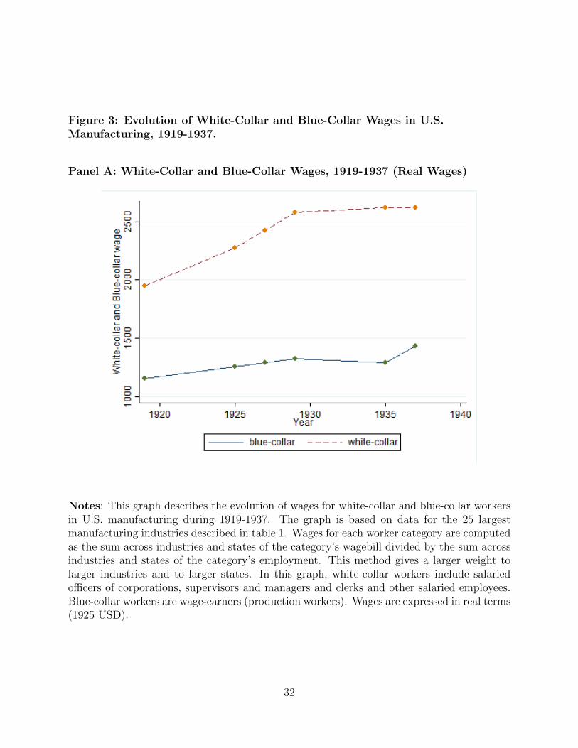
Figure 3: Evolution of White-Collar and Blue-Collar Wages in U.S.Manufacturing, 1919-1937.

Panel A: White-Collar and Blue-Collar Wages, 1919-1937 (Real Wages)

Notes: This graph describes the evolution of wages for white-collar and blue-collar workersin U.S. manufacturing during 1919-1937. The graph is based on data for the 25 largestmanufacturing industries described in table 1. Wages for each worker category are computedas the sum across industries and states of the category’s wagebill divided by the sum acrossindustries and states of the category’s employment. This method gives a larger weight tolarger industries and to larger states. In this graph, white-collar workers include salariedofficers of corporations, supervisors and managers and clerks and other salaried employees.Blue-collar workers are wage-earners (production workers). Wages are expressed in real terms(1925 USD).

32

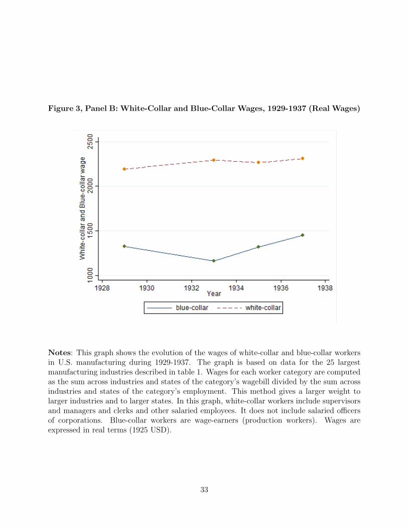
Figure 3, Panel B: White-Collar and Blue-Collar Wages, 1929-1937 (Real Wages)

Notes: This graph shows the evolution of the wages of white-collar and blue-collar workersin U.S. manufacturing during 1929-1937. The graph is based on data for the 25 largestmanufacturing industries described in table 1. Wages for each worker category are computedas the sum across industries and states of the category’s wagebill divided by the sum acrossindustries and states of the category’s employment. This method gives a larger weight tolarger industries and to larger states. In this graph, white-collar workers include supervisorsand managers and clerks and other salaried employees. It does not include salaried officersof corporations. Blue-collar workers are wage-earners (production workers). Wages areexpressed in real terms (1925 USD).

33

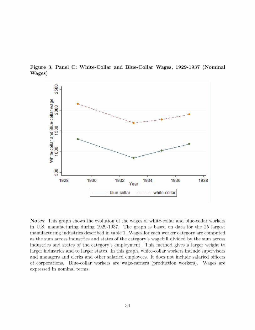
Figure 3, Panel C: White-Collar and Blue-Collar Wages, 1929-1937 (NominalWages)

Notes: This graph shows the evolution of the wages of white-collar and blue-collar workersin U.S. manufacturing during 1929-1937. The graph is based on data for the 25 largestmanufacturing industries described in table 1. Wages for each worker category are computedas the sum across industries and states of the category’s wagebill divided by the sum acrossindustries and states of the category’s employment. This method gives a larger weight tolarger industries and to larger states. In this graph, white-collar workers include supervisorsand managers and clerks and other salaried employees. It does not include salaried officersof corporations. Blue-collar workers are wage-earners (production workers). Wages areexpressed in nominal terms.

34

Figure 4: Evolution of Wage Inequality in U.S. Manufacturing, 1919-1937.

Panel A: Wage Inequality, 1919-1937 (ratio of White-Collar to Blue-Collar Wage

Notes: This graph shows the evolution of the relative wage of white-collar and blue-collarworkers in U.S. manufacturing during 1919-1937. This is the ratio of the two series in figure3, panel A. The graph is based on data for the 25 largest manufacturing industries describedin table 1. Wages for each worker category are computed as the sum across industries andstates of the category’s wagebill divided by the sum industries and states of the category’semployment. This method gives a larger weight to larger industries and to larger states.In this graph, white-collar workers include salaried officers of corporations, supervisors andmanagers and clerks and other salaried employees. Blue-collar workers are wage-earners(production workers).

35

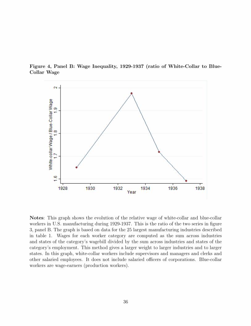
Figure 4, Panel B: Wage Inequality, 1929-1937 (ratio of White-Collar to Blue-Collar Wage

Notes: This graph shows the evolution of the relative wage of white-collar and blue-collarworkers in U.S. manufacturing during 1929-1937. This is the ratio of the two series in figure3, panel B. The graph is based on data for the 25 largest manufacturing industries describedin table 1. Wages for each worker category are computed as the sum across industriesand states of the category’s wagebill divided by the sum across industries and states of thecategory’s employment. This method gives a larger weight to larger industries and to largerstates. In this graph, white-collar workers include supervisors and managers and clerks andother salaried employees. It does not include salaried officers of corporations. Blue-collarworkers are wage-earners (production workers).

36

Figure 5: Evolution of White-Collar and Blue-Collar Employment and Wagesin U.S. Manufacturing, 1929-1937.

Notes: This graph represents the evolution of the employment and wages for white-collarand blue-collar workers in U.S. manufacturing during 1929-1937. The graph is based on datafor the 25 largest manufacturing industries described in table 1. Employment and wages arenormalized to 1 in 1929. Wages for each worker category are computed as the sum acrossindustries and states of the category’s wagebill divided by the sum across industries andstates of the category’s employment. This method gives a larger weight to larger industriesand to larger states. In this graph, white-collar workers include supervisors and managersand clerks and other salaried employees. It does not include salaried officers of corporations.Blue-collar workers are wage-earners (production workers). Wages are expressed in realterms.

37

Figure 6: Evolution of White-Collar and Blue-Collar Employment and Wagesin U.S. Manufacturing by Industry, 1929-1937.

Panel A: Employment

Panel B: Wages

Notes: This graph represents the evolution of the employment and wages for white-collarand blue-collar workers in U.S. manufacturing during 1929-1937 for six selected large indus-tries out of the 25 industries used in this paper. Employment and wages are normalized to1 in 1929. Wages for each worker category are computed as the sum across states of thecategory’s wagebill divided by the sum across states of the category’s employment. Thismethod gives a larger weight to larger states. In this graph, white-collar workers include su-pervisors and managers and clerks and other salaried employees. It does not include salariedofficers of corporations. Blue-collar workers are wage-earners (production workers). Wagesare expressed in real terms.

38

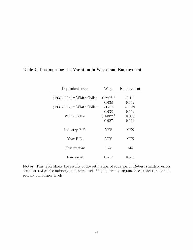
Table 2: Decomposing the Variation in Wages and Employment.

Dependent Var.: Wage Employment

(1933-1935) x White Collar -0.290*** -0.1110.038 0.162

(1935-1937) x White Collar -0.206 -0.0890.038 0.162

White Collar 0.148*** 0.0580.027 0.114

Industry F.E. YES YES

Year F.E. YES YES

Observations 144 144

R-squared 0.517 0.510

Notes: This table shows the results of the estimation of equation 1. Robust standard errorsare clustered at the industry and state level. ***,**,* denote significance at the 1, 5, and 10percent confidence levels.

39

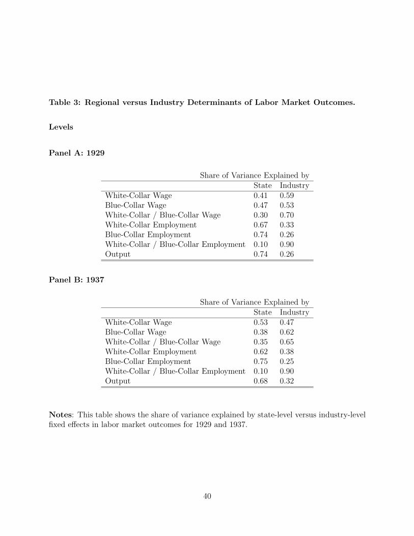
Table 3: Regional versus Industry Determinants of Labor Market Outcomes.

Levels

Panel A: 1929

Share of Variance Explained byState Industry

White-Collar Wage 0.41 0.59Blue-Collar Wage 0.47 0.53White-Collar / Blue-Collar Wage 0.30 0.70White-Collar Employment 0.67 0.33Blue-Collar Employment 0.74 0.26White-Collar / Blue-Collar Employment 0.10 0.90Output 0.74 0.26

Panel B: 1937



Notes: This table shows the share of variance explained by state-level versus industry-levelfixed effects in labor market outcomes for 1929 and 1937.

40

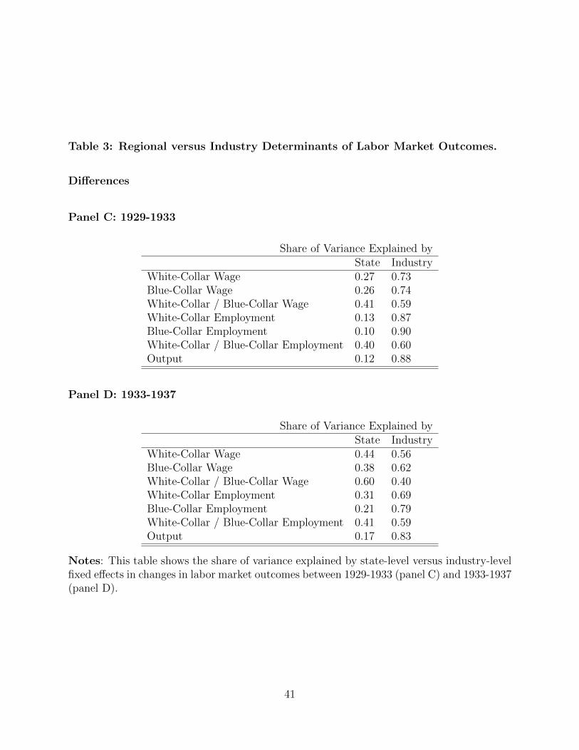
Table 3: Regional versus Industry Determinants of Labor Market Outcomes.

Differences

Panel C: 1929-1933



Panel D: 1933-1937



Notes: This table shows the share of variance explained by state-level versus industry-levelfixed effects in changes in labor market outcomes between 1929-1933 (panel C) and 1933-1937(panel D).

41

Figure 7: Variation in Manufacturing Output by State, 1927-1937.

Notes: This map shows the variation in manufacturing output (revenue) for each of the 48continental states between 1927 and 1937. Darker shades of red represent a larger increase(or a smaller decrease) in output. Manufacturing output in each state is measured as thesum across the 25 largest manufacturing industries described in table 1.

42

Figure 8: Bank Loans in the U.S., 1920-1940.

Notes: This figure shows the evolution of bank loans in the U.S. over 1920-1940. Thedata comes from the Annual Report of the Comptroller of the Currency for each year andcorresponds to “loans and discounts by all active banks (national, state (commercial), savingsand private banks.” The series if for nominal bank loans and is measured in thousands ofmillions of U.S. dollars.

43

Figure 9: Variation in Bank Loans by State, 1929-1933.

Notes: This map shows the variation in total bank loans for each of the 48 continentalstates between 1929 and 1933. Darker shades of blue represent a larger increase (or asmaller decrease) in bank lending. Data on bank loans comes from the Annual Report of theComptroller of the Currency and corresponds to “loans and discounts by all active banks(national, state (commercial), savings and private banks”.

44

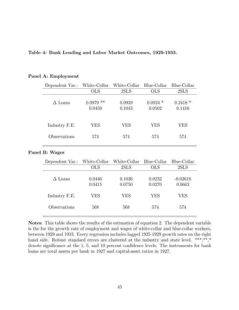
Table 4: Bank Lending and Labor Market Outcomes, 1929-1933.

Panel A: Employment

Dependent Var.: White-Collar White-Collar Blue-Collar Blue-CollarOLS 2SLS OLS 2SLS

∆ Loans 0.0979 ** 0.0939 0.0924 * 0.2418 *0.0459 0.1043 0.0502 0.1416

Industry F.E. YES YES YES YES

Observations 574 574 574 574

Panel B: Wages


∆ Loans 0.0446 0.1036 0.0232 -0.026180.0415 0.0750 0.0270 0.0663



Notes: This table shows the results of the estimation of equation 2. The dependent variableis the for the growth rate of employment and wages of white-collar and blue-collar workers,between 1929 and 1933. Every regression includes lagged 1925-1929 growth rates on the righthand side. Robust standard errors are clustered at the industry and state level. ***,**,*denote significance at the 1, 5, and 10 percent confidence levels. The instruments for bankloans are total assets per bank in 1927 and capital-asset ratios in 1927.

45

Figure 10: New Deal Federal Spending by State.

Notes: This map shows the total amount of New Deal FERA and CWA grants for eachstate. Darker shades represent higher levels of fiscal spending.

46

Table 5: Federal Spending and Labor Market Outcomes, 1933-1937.

Panel A: Employment


Federal Gov. Spending 0.0152 0.1253 0.0325 0.3151*0.0493 0.2332 0.0360 0.1795



Panel B: Wages


Federal Gov. Spending 0.0068 -0.0357 -0.0113 0.03200.0265 0.0840 0.0153 0.0620



Notes: This table shows the results of the estimation of equation 3. The dependent variableis the for the growth rate of employment and wages of white-collar and blue-collar workers,between 1933 and 1937. Every regression includes lagged 1929-1933 growth rates on the righthand side. Robust standard errors are clustered at the industry and state level. ***,**,*denote significance at the 1, 5, and 10 percent confidence levels. The independent variableFederal Gov. Spending represents federal government spending under the New Deal programsFederal Emergency Relief Administration (FERA) and Civil Works Administration (CWA).The instruments for this variable are voter turnout per capita in the 1932 election (normalizedby the population in 1930) and land area, both defined at the state leve as discussed in thetext.

47

Table 6: Educational Attainment of White-Collar and Blue-Collar Workers inManufacturing based on the 1940 Population Census

Share of workers with at least a high-school degree, by stateState Blue-Collar White-Collar State Blue-Collar White-Collar

Alabama 0.13 0.61 Nebraska 0.40 0.67Arizona 0.18 0.85 Nevada 0.00 0.75Arkansas 0.10 0.45 New Hampshire 0.13 0.82California 0.29 0.63 New Jersey 0.13 0.57Colorado 0.19 0.69 New Mexico 0.15 0.50

Connecticut 0.13 0.60 New York 0.12 0.56Delaware 0.17 0.67 North Carolina 0.15 0.68

District of Columbia 0.28 0.77 North Dakota 0.27 0.57Florida 0.19 0.71 Ohio 0.20 0.66Georgia 0.09 0.64 Oklahoma 0.24 0.64Idaho 0.46 0.86 Oregon 0.23 0.69Illinois 0.18 0.60 Pennsylvania 0.15 0.63Indiana 0.25 0.63 Rhode Island 0.10 0.54

Iowa 0.25 0.59 South Carolina 0.13 0.71Kansas 0.25 0.69 South Dakota 0.44 0.64

Kentucky 0.13 0.59 Tennessee 0.17 0.68Louisiana 0.14 0.62 Texas 0.22 0.67

Maine 0.19 0.67 Utah 0.35 0.75Maryland 0.12 0.49 Vermont 0.18 0.47

Massachusetts 0.16 0.68 Virginia 0.16 0.66Michigan 0.18 0.60 Washington 0.25 0.66Minnesota 0.22 0.69 West Virginia 0.29 0.63Mississippi 0.26 0.70 Wisconsin 0.18 0.64Missouri 0.17 0.59 Wyoming 0.20 1.00Montana 0.21 0.33

Notes: This table shows the share of white-collar and blue-collar workers in each state inthe 1940 Population Census with an educational attainment corresponding to at least a highschool degree (12th grade). Workers employed in manufacturing industries were assigned tothe white-collar or blue-collar categories based on their occupation as described in Section2.3.

48

Figure 11: Educational Attainment of White-Collar and Blue-Collar Workersbased on the 1940 Population Census.

Notes: This figure shows the distribution of years of schooling for white-collar and blue-collar workers of ages 20 to 65 in the manufacturing sector. Section 2.3 describes the classi-fication of workers into these categories.

49

Table 7: Data Availability in the Census of Manufactures.

Panel B. Year 1937: Wages

Questionnaire Tabulated - Industry Level

Officers Employees Wage Earners Officers Employees Wage Earners

1929 Yes Yes Yes Yes Yes Yes1931 No No Yes No No Yes1933 Yes Yes Yes No Yes Yes1935 Yes Yes Yes Yes Yes Yes1937 Yes Yes Yes Yes Yes Yes

Notes: This figure shows the availability of different worker categories in each Census ofManufactures during the Depression. The first three columns indicate whether data wasrequested in the Census questionnaire. The next three columns indicate whether there isa tabulation in the Census report providing these data at the industry level. Much of thedata is also available i) at the state level and/or ii) at the industry by state level. Workercategories show in this table are i) salaried officers of corporations, ii) salaried employeesand iii) wage-earners (production workers). More detailed categories are available for someyears, as described in the text.

50

the determinants of u.s. wage inequality during the great

Documents