1

THE DETERMINANTS OF INDUSTRIALIZATION IN DEVELOPING COUNTRIES, 1960-20051

Authors Francesca Guadagno, UNU-MERIT and Maastricht University, guadagno@merit.unu.edu

Abstract

This paper goes back to the Cornwall (1977) model for explaining the role of manufacturing in economic growth and estimates the equation of manufacturing growth. It contributes to the literature on the hypothesis of manufacturing as an engine of growth by an empirical analysis of the determinants of industrialization in 74 countries for the period 1960-2005. Results show that industrialization is faster for larger countries with an undeveloped industrial base and development strategies based on trade openness, undervaluation, skills and knowledge accumulation. In particular, while from 1970 to the mid 90s technological backwardness and undervaluation were the main drivers of industrialization, since 1995 investments in knowledge accumulation have become increasingly crucial. Some robustness checks corroborate the validity of these results.

Key Words: Structural Change, Manufacturing, Innovation, Development

1 This paper is part of my PhD Dissertation. I thank my supervisor, prof. Bart Verspagen, for guidance and suggestions and prof. Jan Fagerberg for comments on a previous version.

2

1 INTRODUCTION It is widely recognized that industrialization, intended as the shift from agriculture to manufacturing, is key to development: hardly any countries have developed without industrializing. This phenomenon has been so striking to induce some economists to hypothesize that the manufacturing sector is the engine of economic growth, the so-called “engine of growth argument” (Kaldor, 1967; Cornwall, 1977).

The debate is quite old and seems outdated if one thinks about the recent success in the service sector. Services have increased their shares in GDP in both developed and developing countries and are increasingly seen as the new engine of growth. In developing countries, the share of services in GDP was already 40% in the 1950s (well higher than the one of manufacturing, 11%) and increased up to 51% in 2005. In advanced economies, the share of services increased even more from the 50s to 2005, going from 43% to 70% (Szirmai, 2011). The Indian case is often brought as an example of successful service-led growth. In India, not only the services sector greatly contributes to GDP, but distinguishes itself for its dynamism since modern services (computer, business, and financial services) are the fastest growing category.

The recent economic crisis, coupled with the considerable expansion of the financial service sector, and the difficulties that many developing countries still encounter to industrialize, brought manufacturing back in the spotlight. Policy makers in both developed and developing countries are reconsidering the virtues of manufacturing. Recent empirical work applied cross country and panel data analysis and found general support to the hypothesis of manufacturing as an engine of growth (among the most recent, Rodrik, 2008; Fagerberg and Verspagen, 1999, 2002; Szirmai, 2011; Szirmai and Verpagen, 2011).

This paper goes back to the Cornwall (1977) model for explaining the role of manufacturing in economic growth and estimates the equation of manufacturing growth. By applying panel data analysis, it looks at the determinants of industrialization in a large sample of developed and developing countries from 1960 to 2005. In this way, it contributes to the structural approach in development economics and to the recent empirical analysis on industrialization and growth. By introducing technical change as an explanatory variable, it also contributes to the evolutionary approach to innovation and development.

In the next section, we briefly review the literature on the role of industrialization for development, the relationship between technical change and economic growth, and the factors behind industrialization. The dataset is described in section 3 where some descriptive statistics are also presented. Section 4 discusses the results of analysis of the determinants of industrialization. In the following section, we expand upon these findings by investigating the role of interdependencies and innovation systems and the evolution of the determinants over different periods. Some robustness checks are reported in section 6. Section 7 briefly concludes.

2 LITERATURE REVIEW AND APPROACH

2.1 Literature review

The term industrialization refers to the structural change that backward countries experience in their development process from an agricultural to an industrial economy, with the profound changes in the society that this entails (Kuznets, 1973). Old development economists observed structural differences between key sectors of the economy and developed models of dual economy with a high productivity, ‘capitalist’, and a low productivity, ‘subsistence’, sector. In this view,

3

development is conditional on the movement of labour to the capitalist sector. In fact, beyond productivity, the manufacturing sector is characterized by economies of scale that, by reducing unit costs, allow increasing output. In turn, the growth of the output of the manufacturing sector impacts the growth rate of the economy via backward and forward linkages to non-manufacturing productivity. Moreover, the manufacturing sector comprises the technology sector, i.e. the sector responsible for the introduction of innovation (Lewis, 1954; Fei and Ranis, 1964; Cornwall, 1977).

Building upon these theories, the technology gap literature, and the studies of the ‘patterns of industrialization’ approach, Cornwall (1977) formulated a model for explaining the role of growth of manufacturing output. Two main equations composed the model:

The first equation explains the output growth in the manufacturing sector and the second the aggregate output growth rate. That the growth of output depends on the rate of growth of manufacturing output, , is reflected in the coefficient, e1, which is exactly the measure of the power of manufacturing as an engine of growth. The determinants of the growth rate of manufacturing output, , are the level and growth rate of aggregate income, income relative to the most developed economies, and investment. The level of income is introduced to take into consideration that, when per capita income rises, consumption shifts from goods to service. A feedback from demand growth is introduced via the income growth rate. The ratio of per capita income compared with that of high-income countries captures the size of the technology gap: the larger the gap with the technological frontier, the greater the amount of technology that an industrializing country can borrow, and so the higher the rate of industrialization. Investments measure the efforts to develop borrowed and indigenous technologies. Estimations of this model for the market economies revealed the importance of the manufacturing sector, flexibility (the ability of the economy to shift towards manufacturing activities), and investments.

Most recent empirical work partially confirmed the engine of growth hypothesis (Tregenna, 2007; Kuturia and Raj, 2009; Szirmai, 2009; Timmer and de Vries, 2009). On the one hand, in developing countries, manufacturing is still relevant as an engine of growth when the most dynamic industries are targeted and investments in skills are undertaken. On the other hand, in developed countries manufacturing is not anymore an engine of growth (Fagerberg and Verspagen, 1999; Szirmai and Verspagen, 2011).

Fagerberg and Verspagen (1999) updated and extended upon the work of Cornwall (1977) by using a larger sample of countries for the period 1973-1990. They find that, in market economies, the effect of manufacturing on growth had vanished; newly-industrializing countries are instead those that benefit more from expansions of the manufacturing sector. They test for the importance of the most dynamic segments of the manufacturing sector (as theorized by Cornwall) and confirm the importance of flexibility to shift towards manufacturing productions. Szirmai and Verspagen (2011) study 88 countries for the period 1950-2005 and find that manufacturing had a direct effect on growth only from 1970 to 1990. Since 1990, the positive effect of manufacturing on growth in developing countries has become more and more dependent on skills’ accumulation.

These contributions refer implicitly or explicitly to technical change. What has been said about the relationship between technical change and economic growth?

For a quite long period in economic theory, technical change was conceived as “any kind of shift in the production function” (Solow, 1957). Thanks to the vagueness of this idea, technological progress could be called “residual”, i.e. what is left of GDP growth after accounting for labour and capital growth (total factor productivity), or “measure of our ignorance”. Solow and the other

4

economists who contributed to the field of neoclassical growth theory introduced it as an exogenous variable and did not spend much effort into opening this “black box”.

Following these theories, technological progress was commonly viewed as a typical first-world activity that has to do with developing new solutions via the exploitation of advanced knowledge and techniques. So, in an international perspective, what backward countries need in order to (more or less automatically) converge is accumulating capital. Due to the nature of public good of knowledge, the process of acquisition of capital (and so of technology and knowledge attached to it) was regarded as essentially automatic (Veblen, 1915).

However, if it is so automatic, why do economists observe divergence rather than converge between developed and developing countries?

Notwithstanding the availability of advanced machines and techniques, technology transfer is still burdensome as it requires investments in physical, financial, and institutional infrastructure (Gerschenkron, 1962) and efforts to build different types of capabilities (e.g. social capabilities by Abramovitz, 1986; absorptive capacity by Cohen and Levinthal, 1990; technological capabilities by Kim, 1980 and Lall, 1992).

Nelson and Pack (1999) develop a model to explain the so-called “Asian miracle”. According to their analysis, high physical investments and initial conditions are not enough to explain Asian performance. Absorption of modern technologies and structural change were critical ingredients of the Asian development process. According to the authors, such technological effort does not take the form of formal R&D, but rather of “efforts of firm to learn about new opportunities, improve organization and inventory management, and undertake minor bur cumulatively significant changes in production processes” (p. 431). The former quote demonstrates how hard it is to capture technological change.

Innovation is so complex that some scholars describe it as a systemic phenomenon determined by the interactions of a wide range of factors (geographical, social, historical, political, and so on). The coevolution of all these factors shape the evolution of capabilities and the chances of successful innovative performances of countries, regions, and sectors (the so-called system of innovation approach, as firstly theorized by Freeman, 1987; Nelson, 1993, Lundvall, 1993). At the empirical level, a great deal of studies tested the role of innovation and innovation system for growth and development.2

Among the others, Fagerberg and Srholec (2008) explored 115 countries in two periods, 1992-1994 and 2002-2004, and identified 4 main factors capturing different aspects of capabilities: innovation system, governance, political system, and openness. Results demonstrate that catching up is positively affected only by developed innovation systems and good governance, while openness to trade, FDI ,and the political system do not matter much for development.

2.2 Approach

As the literature review has pointed out, research focused on the relationship between growth and industrialization, but why do some countries industrialize and some others do not? And, which is the role of technical change in explaining differences in industrialization? Moreover, if innovation has a systemic nature, does the role of innovation depend on the interplay of different factors and characteristics of the country in question? Finally, the global scenario in which countries industrialize is constantly changing. How did the determinants of industrialization change over time? In other words, how do developing countries need to adapt their development strategies in order to meet the evolving conditions for industrialization? 2 For an extensive review of the literature about innovation and development, see Fagerberg et al. (2010).

5

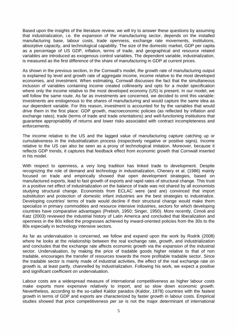
Based upon the insights of the literature review, we will try to answer these questions by assuming that industrialization, i.e. the expansion of the manufacturing sector, depends on the installed manufacturing base, labour costs, trade openness, exchange rate movements, institutions, absorptive capacity, and technological capability. The size of the domestic market, GDP per capita as a percentage of US GDP, inflation, terms of trade, and geographical and resource related variables are introduced as exogenous control variables. The dependent variable, industrialization, is measured as the first difference of the share of manufacturing in GDP at current prices.

As shown in the previous section, in the Cornwall’s model, the growth rate of manufacturing output is explained by level and growth rate of aggregate income, income relative to the most developed economies, and investment. When estimating, Cornwall discusses the fact that the simultaneous inclusion of variables containing income created collinearity and opts for a model specification where only the income relative to the most developed economy (US) is present. In our model, we will follow the same route. As far as investments are concerned, we decided to omit this variable: investments are endogenous to the shares of manufacturing and would capture the same idea as our dependent variable. For this reason, investment is accounted for by the variables that would drive them in the first place: GDP growth, macroeconomic policies (as reflected by inflation and exchange rates), trade (terms of trade and trade orientations) and well-functioning institutions that guarantee appropriability of returns and lower risks associated with contract incompleteness and enforcements.

The income relative to the US and the lagged value of manufacturing capture catching up or cumulativeness in the industrialization process (respectively negative or positive signs). Income relative to the US can also be seen as a proxy of technological imitation. Moreover, because it reflects GDP trends, it captures that feedback effect from economic growth that Cornwall inserted in his model.

With respect to openness, a very long tradition has linked trade to development. Despite recognizing the role of demand and technology in industrialization, Chenery et al. (1986) mainly focused on trade and empirically showed that open development strategies, based on manufactured exports, lead to fast growth of exports and rapid rates of structural change. This trust in a positive net effect of industrialization on the balance of trade was not shared by all economists studying structural change. Economists from ECLAC were (and are) convinced that import substitution and protection of domestic infant industries are the best strategies to industrialize. Developing countries’ terms of trade would decline if their structural change would make them specialize in primary commodities and resource intensive industries, sectors for which developing countries have comparative advantages (Prebish, 1950; Singer, 1950). More recently, Cimoli and Katz (2003) reviewed the industrial history of Latin America and concluded that liberalization and openness in the 80s killed the progresses achieved by inward-oriented policies from the 30s to the 80s especially in technology intensive sectors.

As far as undervaluation is concerned, we follow and expand upon the work by Rodrik (2008) where he looks at the relationship between the real exchange rate, growth, and industrialization and concludes that the exchange rate affects economic growth via the expansion of the industrial sector. Undervaluation, by making the price of tradable goods higher relative to that of non tradable, encourages the transfer of resources towards the more profitable tradable sector. Since the tradable sector is mainly made of industrial activities, the effect of the real exchange rate on growth is, at least partly, channelled by industrialization. Following his work, we expect a positive and significant coefficient on undervaluation.

Labour costs are a widespread measure of international competitiveness as higher labour costs make exports more expensive relatively to import, and so slow down economic growth. Nevertheless, according to the so-called Kaldor paradox (Kaldor, 1978) countries with the fastest growth in terms of GDP and exports are characterized by faster growth in labour costs. Empirical studies showed that price competitiveness per se is not the major determinant of international

6

competitiveness in the long run (Fagerberg, 1988; Amendola et al., 1993; Fagerberg et al., 2007). Depending on countries’ industrial specialization, low wages might even be linked to low productivity, and so to lower competitiveness and growth. Even though the sign on the wage variable might vary across sectors, overall the effect of labour costs is expected to be negative (Amable and Verspagen, 1995).

In their work on the hypothesis of manufacturing as an engine of growth, Fagerberg and Verspagen (1999) and Szirmai and Verspagen (2011) introduce respectively education and R&D expenditures and education alone to account for human capital accumulation and ‘innovation systems’ characteristics. We conform to these studies and expect a positive effect of education and technical change on industrialization.

While there is large consensus that institutions matter for growth, this paper tests whether institutions impact on growth via industrialization. Institutions have often come to embrace a mare magnum of concepts. Nelson and Sampat (2001) stress the need for a definition that would make sense of them as a factor shaping economic growth. Fagerberg and Schrolec (2008) distinguish between political system and “quality of governance” variables. The former relates to measures of democracy and rights; the latter to aspects like the easiness of starting and conducting a business. Their results show that good governance matters for growth, while political systems matter only for richer countries. Even though we are deeply persuaded by the idea that institutions are to be accurately defined in relation to the specific phenomena they are meant to explain and that good governance contributes more than democratic political systems, we are confronted with the fact that these indicators are not available for long time series. So, in order to preserve the length of our panel, we chose to rely on political systems variables.

Geographical and resource-related variables are the classic instruments in empirical studies on institutions and growth (e.g., Acemoglu et al., 2001; Dollar and Kraay, 2003; Lee and Kim, 2009). While economic growth theory has focussed on physical and human capital accumulation and technical change, empirical studies argued that these are at best proximate causes of economic growth. This strand of literature identifies trade, institutions, and geography as deeper determinants of economic growth. However, if institutions and trade are endogenous, insomuch as they are mutually shaped and in turn influenced by economic growth, geography is an exogenous determinant of economic growth. Its relation with growth is both direct, because it influences agricultural productivity, health conditions, and resource endowments, and indirect via the effect on trade and institutions (Rodrik et al., 2004).

By creating uncertainty, volatile inflation and terms of trade influence investment choices. Theoretical literature has studied the impact of uncertainty on growth, as channelled by investments. In empirical studies, Fagerberg and Verspagen (1999) introduced inflation as an instrumental variable and Rodrik (2008) used both inflation and terms of trade as additional exogenous covariates of economic growth when the role of manufacturing is analysed. Rodrik finds a negative and significant relationship between growth and inflation in developing countries. Kosakoff and Ramos (2009) described the impact of inflation on the manufacturing sector in Argentina and how investment decisions and capability accumulation of firms are hampered in high-inflationary contexts.

3 OVERVIEW OF THE DATA

3.1 Description of the dataset

Data on the share of manufacturing in GDP, population, openness, human capital, and geography come from the Szirmai and Verspagen database (Szirmai and Verspagen, 2011). In particular, the

7

size of the market (POP) is captured by the logarithm of the population; trade policies by the openness index (exports plus imports as percentage of GDP), and human capital (EDU) by the average years of schooling for the population of above 15 years of age. Two variables capture geography: OIL is a dummy variable that indicates the presence of oil in the country and KGATEMP refers to the climatic zone and is measured as the percentage of land in a temperate climatic zone, transformed in a binary variable.

Data on wages (WAGE) come from the UNIDO Industrial Statistics Database (INDSTAT2 2011 ISIC Rev.3).3 Exchange rate movements are represented by the index UNDERV, which is built by following Rodrik (2008) and using the Penn World Table (version 7.0, update June 2011). This index, taken in logarithmic form, is positive when the currency is undervalued. Data on the terms of trade (TOT) also come from the PWT 7.0. For inflation (INFL) we rely on WDI (2011).4

Our preferred measure of institutions (DEM) is the Vanhanen index (Vanhanen, 2000), that compared to other measures, uses indicators taken from quantitative data and not on subjective evaluations, as the Polity and Freedom House data. The index is built in such a way that low values correspond to low levels of democracy. Data come from the Quality of Government Dataset (version of 11/04/2011).

As measures of technical change, we use indicators based on patents and R&D expenditures. Patent data come from USPTO and WIPO. Data on R&D expenditures over GDP come from the CANA dataset (Castellacci and Natera, 2011).5 In a first stage, we rely on the number of patents per capita at USPTO (PATPC). USPTO patents are the most widely used proxy in the literature, due to their clear advantage in terms of data availability and cross-country comparability. However, the high degree of novelty required by the USPTO does not match with our idea of innovation effort in developing countries. This is why, in a second stage, we explore other indicators: the number of patent per capita granted by national patents’ offices to residents (NATPATPC), R&D expenditures as a percentage of GDP (R&D) and a measure of technological level developed by Fagerberg (1988). This measure of technological level (TL) is attractive insofar as it is constructed as the average of both patents and R&D expenditures (weighted by their standard deviations). National patent offices’ criteria to grant a patent are much less stringent than USPTO’s, so, by using national patents, a much broader range of innovations would be captured.

As for R&D, data for most of the developing countries start in 1980, so the length of the panel is strongly damaged by the introduction of this variable. Notwithstanding this downside, R&D intensity is a very good indicator of innovation especially for developing countries which might need a lengthy process of knowledge accumulation and capability building before filing a patent application. In fact, even though the correlation of patents and R&D expenditures is very high (in agreement with the literature), it is lower for less developed countries.6

3 Values of wage and salaries (at current prices) have been divided by employment (number of persons engaged and number of employees).

4 Gaps have been filled in with the IMF WEO dataset (version of 1999 and 2011) and in the case of Chile and UK with national data sources (respectively, Banco Centrale de Chile and Office of National Statistics).

5 WIPO data start in 1965 and do not include some countries among which Taiwan. Data on R&D expenditures for Taiwan and Korea were retrieved from other sources (OECD; Taiwan National Science Council; Lederman and Saenz, 2005).

6 The correlation between USPTO patents and R&D expenditures as a percentage of GDP is 0.86 for the whole sample but for African countries it decreases to 0.62, and for Latin America to 0.31. The same is true for national offices’ patents: the overall correlation between USPTO and national offices’ patents is 0.74 overall, for Africa is 0.84, but for Asia is around 0.6, and for Latin America 0.2.

8

The resulting dataset is an unbalanced panel of 74 (developed and developing) countries covering the period 1960-2004. Yearly data have been averaged into 9 5-year periods. The sample varies per period, depending on data availability.

3.2 Descriptive statistics

Before delving into the econometric analysis, it is useful to look at the descriptive statistics of our data. This will guide the choice of the type of model to adopt.

Table 1. Descriptive statistics

Variable Mean Standard Deviation Observations

Overall Between Within N n T-bar

First difference of the Manufacturing share in GDP 0.099 2.99 1.32 2.72 650 91 7.14

Lagged value of the Manufacturing share in GDP 18.12 8.32 7.49 4.06 681 91 7.48

Wage (ln) -1.12 1.25 1.03 0.78 561 80 7.01

Population (ln) 9.29 1.66 1.65 028 810 91 8.9

Openness 65.77 42.85 37.89 20.07 787 91 8.65

Undervaluation Index 0.008 0.296 0.066 0.287 702 85 8.26

Democracy Index 14.36 13.41 12.29 5.51 748 89 8.4

Education 5.622 2.793 2.477 1.378 737 85 8.7

GDP per capita as a percentage of US GDP 0.314 .282 0.277 0.065 734 85 8.6

Terms of trade (ln) 0.002 0.103 0.083 0.068 718 85 8.45

Inflation (ln) 2.004 1.25 0.83 0.96 652 83 7.85

USPTO patents per capita 0.015 0.04 0.037 0.017 776 90 8.62

National offices’ patents per capita 0.0522 0.111 0.084 0.062 528 78 6.77

R&D as a percentage of GDP 0.844 0.902 0.884 0.257 309 64 4.82

Depreciated stock of USPTO patents 0.091 0.283 0.27 0.09 753 84 8.96

The table shows that the within component of the standard deviation of the dependent variable, the first difference of the manufacturing share in GDP, is larger than the between component. The

9

opposite is true for all the explanatory variables but inflation and undervaluation (these variables are generally characterized by high volatility).

Following the reasoning in Szirmai and Verspagen (2011), we would rather not rely on a fixed effect model that wipes out between effects because the highest degree of variation in our data comes from the between rather than the within component. Moreover, if the objective of this analysis is to understand why some countries industrialized and some others did not it is clear that our interest lies more in between countries variation rather than within country variation.

Relying on USPTO patent data would be the most conservative choice as its average is the lowest of the proxies of technological efforts. Nevertheless, a clear reason to prefer USPTO data relates to data availability (see number of countries and average number of observations per country, T-bar).

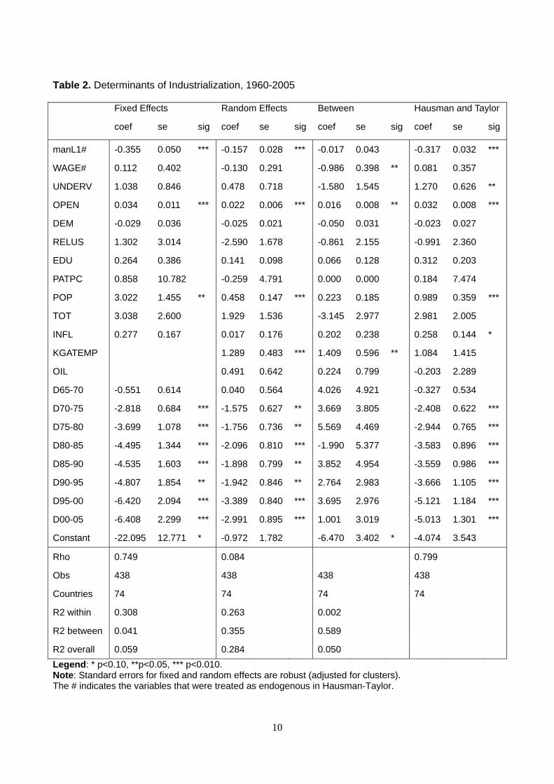
4 RESULTS Our econometric analysis starts with fixed and random effects, between and Hausman and Taylor (1981) estimations. Results are reported in table 2. Following Baltagi et al. (2003), Jacob and Osang (2007) and Szirmai and Verspagen (2011), we separately inspected each single explanatory variable by means of Hausman tests (not reported here) in order to identify which variables are endogenous. Tests showed that ManL1 and WAGE are endogenous. The dependent variable is the first difference of the share of manufacturing in GDP.

10

Table 2. Determinants of Industrialization, 1960-2005

Fixed Effects Random Effects Between Hausman and Taylor

coef se sig coef se sig coef se sig coef se sig

manL1# -0.355 0.050 *** -0.157 0.028 *** -0.017 0.043 -0.317 0.032 ***

WAGE# 0.112 0.402 -0.130 0.291 -0.986 0.398 ** 0.081 0.357

UNDERV 1.038 0.846 0.478 0.718 -1.580 1.545 1.270 0.626 **

OPEN 0.034 0.011 *** 0.022 0.006 *** 0.016 0.008 ** 0.032 0.008 ***

DEM -0.029 0.036 -0.025 0.021 -0.050 0.031 -0.023 0.027

RELUS 1.302 3.014 -2.590 1.678 -0.861 2.155 -0.991 2.360

EDU 0.264 0.386 0.141 0.098 0.066 0.128 0.312 0.203

PATPC 0.858 10.782 -0.259 4.791 0.000 0.000 0.184 7.474

POP 3.022 1.455 ** 0.458 0.147 *** 0.223 0.185 0.989 0.359 ***

TOT 3.038 2.600 1.929 1.536 -3.145 2.977 2.981 2.005

INFL 0.277 0.167 0.017 0.176 0.202 0.238 0.258 0.144 *

KGATEMP 1.289 0.483 *** 1.409 0.596 ** 1.084 1.415

OIL 0.491 0.642 0.224 0.799 -0.203 2.289

D65-70 -0.551 0.614 0.040 0.564 4.026 4.921 -0.327 0.534

D70-75 -2.818 0.684 *** -1.575 0.627 ** 3.669 3.805 -2.408 0.622 ***

D75-80 -3.699 1.078 *** -1.756 0.736 ** 5.569 4.469 -2.944 0.765 ***

D80-85 -4.495 1.344 *** -2.096 0.810 *** -1.990 5.377 -3.583 0.896 ***

D85-90 -4.535 1.603 *** -1.898 0.799 ** 3.852 4.954 -3.559 0.986 ***

D90-95 -4.807 1.854 ** -1.942 0.846 ** 2.764 2.983 -3.666 1.105 ***

D95-00 -6.420 2.094 *** -3.389 0.840 *** 3.695 2.976 -5.121 1.184 ***

D00-05 -6.408 2.299 *** -2.991 0.895 *** 1.001 3.019 -5.013 1.301 ***

Constant -22.095 12.771 * -0.972 1.782 -6.470 3.402 * -4.074 3.543

Rho 0.749 0.084 0.799

Obs 438 438 438 438

Countries 74 74 74 74

R2 within 0.308 0.263 0.002

R2 between 0.041 0.355 0.589

R2 overall 0.059 0.284 0.050 Legend: * p<0.10, **p<0.05, *** p<0.010. Note: Standard errors for fixed and random effects are robust (adjusted for clusters). The # indicates the variables that were treated as endogenous in Hausman-Taylor.

11

Lagged manufacturing, size of domestic market, and trade openness are clear determinants of industrialization. WAGE is positive but not significant in fixed effects and Hausman and Taylor and becomes negative and significant in the between specification. Undervaluation and inflation are positive and significant only in the Hausman and Taylor estimation. Democracy is always negative and never significant. USPTO patents, education, and RELUS are never significant and sometimes have unexpected signs. KGATEMP is positive and significant only in the random effects and between specifications. All period dummies but the first are significant in all specifications except for the between specification. Note that these results are robust to the inclusion of continent dummies and to the simultaneous inclusion of both period and continent dummies (estimations not reported here).

The coefficients on the period dummies suggest that industrializing has become harder over time. A significance test on whether the coefficients on the period dummies are different from each other indicates that periods from 1970 to 1995 and periods 1995-2005 could be unified because the coefficients are not significantly different from each other.

The Hausman test strongly rejects (p=0.0000) the null hypothesis of not significant differences between the fixed and random effects model and so discourages from using random effects which would have been our preferred choice given the nature of the data. This is why the Hausman and Taylor model is chosen and from now on only Hausman and Taylor results will be shown. The model by Hausman and Taylor combines the advantages of fixed and random effects models because it allows country effects to be correlated with the explanatory variables and does not eliminate country time-invariant effects. Nevertheless, in the presence of lagged regressors, the Hausman and Taylor estimator is inconsistent (and so are both fixed and random effects estimators). In section 6.1, we will use the GMM approach to validate our results.

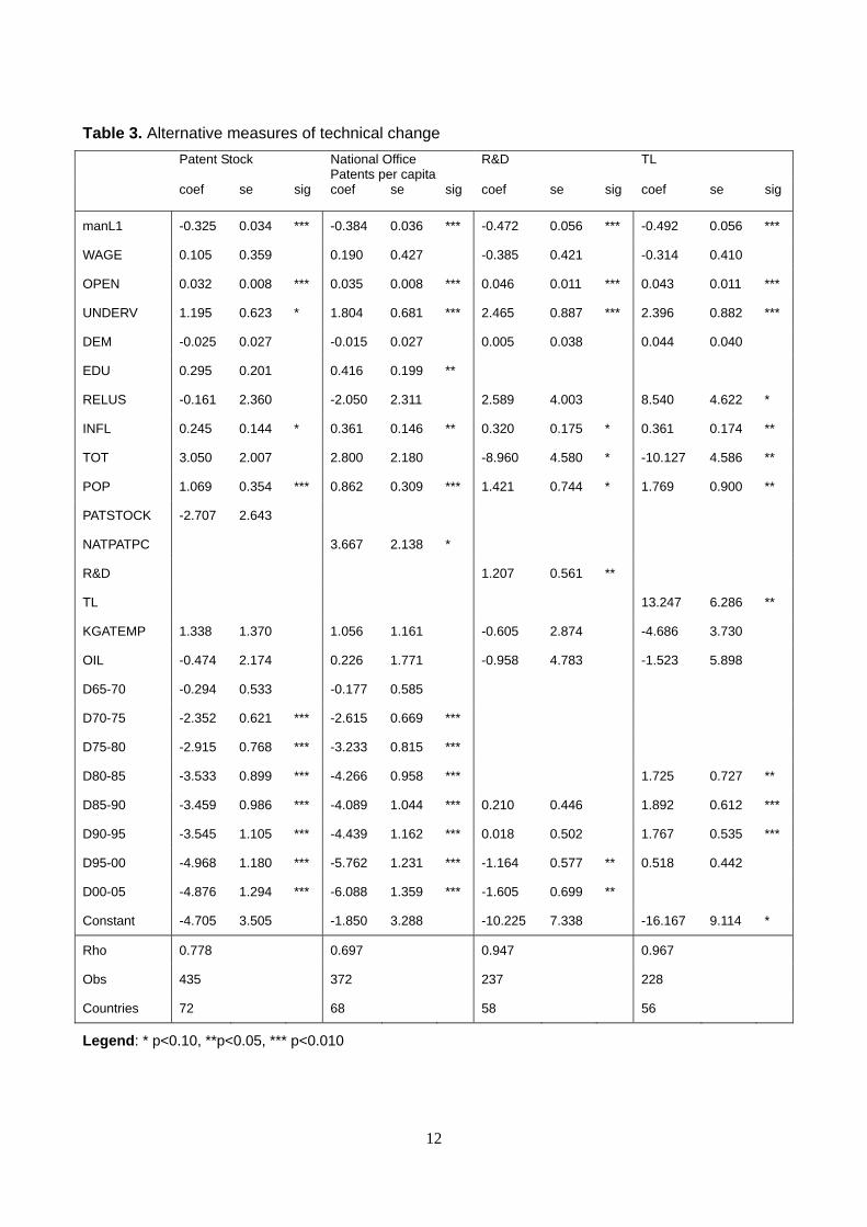
Moved by the suspect that USPTO patents per capita do not fully capture technological efforts in developing countries, we employ different measures of innovation. Table 3 reports Hausman and Taylor estimation where we test four alternative measures of technical change: the depreciated USPTO patent stock (introduced as a comparison to the other models), patents granted to residents by national patent offices, R&D expenditures over GDP, and an indicator of technological level developed by Fagerberg (1988).

As for the previous estimation, we run Hausman tests to check which of these variables are endogenous. The tests indicate exogeneity of patent stock and patents granted by the national patent offices and endogeneity of R&D and the technological level. As suggested by Fagerberg and Verspagen (1999), education has been dropped in columns 3 and 4 because R&D and secondary education are too closely related.

12

Table 3. Alternative measures of technical change Patent Stock National Office

Patents per capita R&D TL

coef se sig coef se sig coef se sig coef se sig

manL1 -0.325 0.034 *** -0.384 0.036 *** -0.472 0.056 *** -0.492 0.056 ***

WAGE 0.105 0.359 0.190 0.427 -0.385 0.421 -0.314 0.410

OPEN 0.032 0.008 *** 0.035 0.008 *** 0.046 0.011 *** 0.043 0.011 ***

UNDERV 1.195 0.623 * 1.804 0.681 *** 2.465 0.887 *** 2.396 0.882 ***

DEM -0.025 0.027 -0.015 0.027 0.005 0.038 0.044 0.040

EDU 0.295 0.201 0.416 0.199 **

RELUS -0.161 2.360 -2.050 2.311 2.589 4.003 8.540 4.622 *

INFL 0.245 0.144 * 0.361 0.146 ** 0.320 0.175 * 0.361 0.174 **

TOT 3.050 2.007 2.800 2.180 -8.960 4.580 * -10.127 4.586 **

POP 1.069 0.354 *** 0.862 0.309 *** 1.421 0.744 * 1.769 0.900 **

PATSTOCK -2.707 2.643

NATPATPC 3.667 2.138 *

R&D 1.207 0.561 **

TL 13.247 6.286 **

KGATEMP 1.338 1.370 1.056 1.161 -0.605 2.874 -4.686 3.730

OIL -0.474 2.174 0.226 1.771 -0.958 4.783 -1.523 5.898

D65-70 -0.294 0.533 -0.177 0.585

D70-75 -2.352 0.621 *** -2.615 0.669 ***

D75-80 -2.915 0.768 *** -3.233 0.815 ***

D80-85 -3.533 0.899 *** -4.266 0.958 *** 1.725 0.727 **

D85-90 -3.459 0.986 *** -4.089 1.044 *** 0.210 0.446 1.892 0.612 ***

D90-95 -3.545 1.105 *** -4.439 1.162 *** 0.018 0.502 1.767 0.535 ***

D95-00 -4.968 1.180 *** -5.762 1.231 *** -1.164 0.577 ** 0.518 0.442

D00-05 -4.876 1.294 *** -6.088 1.359 *** -1.605 0.699 **

Constant -4.705 3.505 -1.850 3.288 -10.225 7.338 -16.167 9.114 *

Rho 0.778 0.697 0.947 0.967

Obs 435 372 237 228

Countries 72 68 58 56

Legend: * p<0.10, **p<0.05, *** p<0.010

13

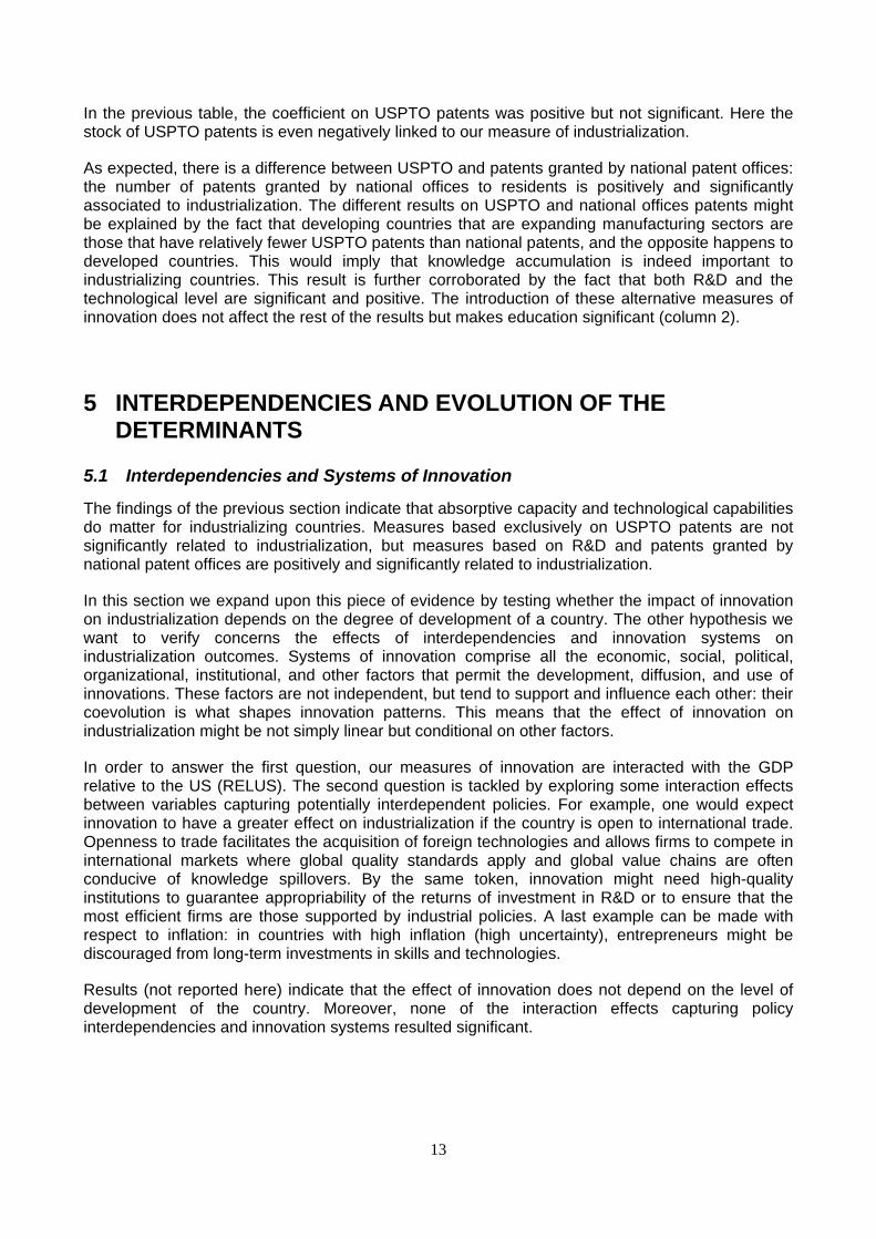
In the previous table, the coefficient on USPTO patents was positive but not significant. Here the stock of USPTO patents is even negatively linked to our measure of industrialization.

As expected, there is a difference between USPTO and patents granted by national patent offices: the number of patents granted by national offices to residents is positively and significantly associated to industrialization. The different results on USPTO and national offices patents might be explained by the fact that developing countries that are expanding manufacturing sectors are those that have relatively fewer USPTO patents than national patents, and the opposite happens to developed countries. This would imply that knowledge accumulation is indeed important to industrializing countries. This result is further corroborated by the fact that both R&D and the technological level are significant and positive. The introduction of these alternative measures of innovation does not affect the rest of the results but makes education significant (column 2).

5 INTERDEPENDENCIES AND EVOLUTION OF THE DETERMINANTS

5.1 Interdependencies and Systems of Innovation

The findings of the previous section indicate that absorptive capacity and technological capabilities do matter for industrializing countries. Measures based exclusively on USPTO patents are not significantly related to industrialization, but measures based on R&D and patents granted by national patent offices are positively and significantly related to industrialization.

In this section we expand upon this piece of evidence by testing whether the impact of innovation on industrialization depends on the degree of development of a country. The other hypothesis we want to verify concerns the effects of interdependencies and innovation systems on industrialization outcomes. Systems of innovation comprise all the economic, social, political, organizational, institutional, and other factors that permit the development, diffusion, and use of innovations. These factors are not independent, but tend to support and influence each other: their coevolution is what shapes innovation patterns. This means that the effect of innovation on industrialization might be not simply linear but conditional on other factors.

In order to answer the first question, our measures of innovation are interacted with the GDP relative to the US (RELUS). The second question is tackled by exploring some interaction effects between variables capturing potentially interdependent policies. For example, one would expect innovation to have a greater effect on industrialization if the country is open to international trade. Openness to trade facilitates the acquisition of foreign technologies and allows firms to compete in international markets where global quality standards apply and global value chains are often conducive of knowledge spillovers. By the same token, innovation might need high-quality institutions to guarantee appropriability of the returns of investment in R&D or to ensure that the most efficient firms are those supported by industrial policies. A last example can be made with respect to inflation: in countries with high inflation (high uncertainty), entrepreneurs might be discouraged from long-term investments in skills and technologies.

Results (not reported here) indicate that the effect of innovation does not depend on the level of development of the country. Moreover, none of the interaction effects capturing policy interdependencies and innovation systems resulted significant.

14

5.2 Evolution of the determinants of industrialization

In this section we will explore if, and how, the determinants of industrialization changed over time, i.e. we will investigate whether the estimated coefficients are constant over time. According to our data, between 1960 and 1975 the share of manufacturing increased in the developing world, but decreased in developed countries. After 1975 only Asia continued to experience an expansion of the manufacturing sector, while Africa and Latin America were deindustrializing (Szirmai, 2011). This evidence suggests that differences in the power of our determinants are likely to emerge from this analysis.

Furthermore, section 3 of this paper evidenced that industrialization became increasingly difficult as the coefficients of the time dummies were significant, negative, and decreasing over periods. Tests on whether the coefficients of the time dummies are significantly different from each other showed that coefficients for the periods ranging from 1970 to 1995 and from 1995 to 2005 could be unified.

In this analysis the original 9 periods will be aggregated into 3 sub-periods: 1960-1970, 1970-1995 and 1995-2005. Slope dummies for these 3 sub-periods are created and interacted with all the explanatory variables. Four models will be estimated: the base model, a model with patents per capita granted from national offices to residents (NATPATPC), one with R&D and the last with the index of technological level (TL). In each of these models, the coefficient on each variable will be interacted with time dummies for each of the three sub-periods. Therefore, three coefficients per variable are reported.

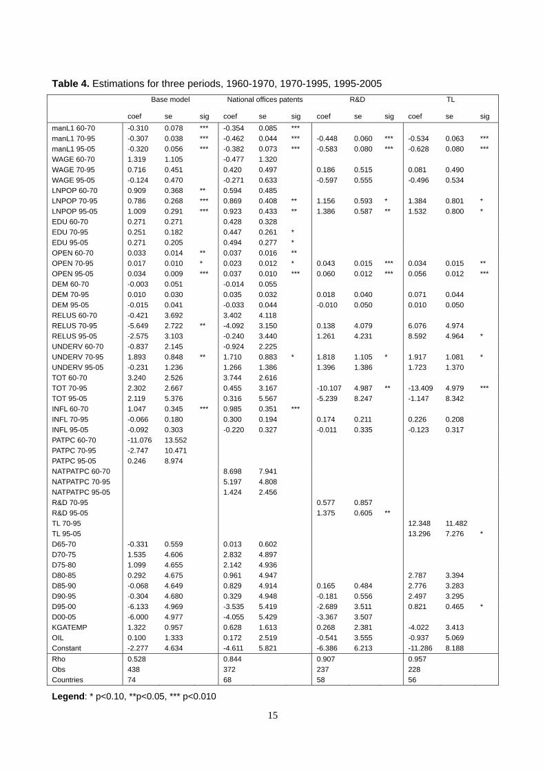
Table 4 present Hausman and Taylor estimations for these four specifications.

15

Table 4. Estimations for three periods, 1960-1970, 1970-1995, 1995-2005 Base model National offices patents R&D TL

coef se sig coef se sig coef se sig coef se sig manL1 60-70 -0.310 0.078 *** -0.354 0.085 *** manL1 70-95 -0.307 0.038 *** -0.462 0.044 *** -0.448 0.060 *** -0.534 0.063 *** manL1 95-05 -0.320 0.056 *** -0.382 0.073 *** -0.583 0.080 *** -0.628 0.080 *** WAGE 60-70 1.319 1.105 -0.477 1.320 WAGE 70-95 0.716 0.451 0.420 0.497 0.186 0.515 0.081 0.490 WAGE 95-05 -0.124 0.470 -0.271 0.633 -0.597 0.555 -0.496 0.534 LNPOP 60-70 0.909 0.368 ** 0.594 0.485 LNPOP 70-95 0.786 0.268 *** 0.869 0.408 ** 1.156 0.593 * 1.384 0.801 * LNPOP 95-05 1.009 0.291 *** 0.923 0.433 ** 1.386 0.587 ** 1.532 0.800 * EDU 60-70 0.271 0.271 0.428 0.328 EDU 70-95 0.251 0.182 0.447 0.261 * EDU 95-05 0.271 0.205 0.494 0.277 * OPEN 60-70 0.033 0.014 ** 0.037 0.016 ** OPEN 70-95 0.017 0.010 * 0.023 0.012 * 0.043 0.015 *** 0.034 0.015 ** OPEN 95-05 0.034 0.009 *** 0.037 0.010 *** 0.060 0.012 *** 0.056 0.012 *** DEM 60-70 -0.003 0.051 -0.014 0.055 DEM 70-95 0.010 0.030 0.035 0.032 0.018 0.040 0.071 0.044 DEM 95-05 -0.015 0.041 -0.033 0.044 -0.010 0.050 0.010 0.050 RELUS 60-70 -0.421 3.692 3.402 4.118 RELUS 70-95 -5.649 2.722 ** -4.092 3.150 0.138 4.079 6.076 4.974 RELUS 95-05 -2.575 3.103 -0.240 3.440 1.261 4.231 8.592 4.964 * UNDERV 60-70 -0.837 2.145 -0.924 2.225 UNDERV 70-95 1.893 0.848 ** 1.710 0.883 * 1.818 1.105 * 1.917 1.081 * UNDERV 95-05 -0.231 1.236 1.266 1.386 1.396 1.386 1.723 1.370 TOT 60-70 3.240 2.526 3.744 2.616 TOT 70-95 2.302 2.667 0.455 3.167 -10.107 4.987 ** -13.409 4.979 *** TOT 95-05 2.119 5.376 0.316 5.567 -5.239 8.247 -1.147 8.342 INFL 60-70 1.047 0.345 *** 0.985 0.351 *** INFL 70-95 -0.066 0.180 0.300 0.194 0.174 0.211 0.226 0.208 INFL 95-05 -0.092 0.303 -0.220 0.327 -0.011 0.335 -0.123 0.317 PATPC 60-70 -11.076 13.552 PATPC 70-95 -2.747 10.471 PATPC 95-05 0.246 8.974 NATPATPC 60-70 8.698 7.941 NATPATPC 70-95 5.197 4.808 NATPATPC 95-05 1.424 2.456 R&D 70-95 0.577 0.857 R&D 95-05 1.375 0.605 ** TL 70-95 12.348 11.482 TL 95-05 13.296 7.276 * D65-70 -0.331 0.559 0.013 0.602 D70-75 1.535 4.606 2.832 4.897 D75-80 1.099 4.655 2.142 4.936 D80-85 0.292 4.675 0.961 4.947 2.787 3.394 D85-90 -0.068 4.649 0.829 4.914 0.165 0.484 2.776 3.283 D90-95 -0.304 4.680 0.329 4.948 -0.181 0.556 2.497 3.295 D95-00 -6.133 4.969 -3.535 5.419 -2.689 3.511 0.821 0.465 * D00-05 -6.000 4.977 -4.055 5.429 -3.367 3.507 KGATEMP 1.322 0.957 0.628 1.613 0.268 2.381 -4.022 3.413 OIL 0.100 1.333 0.172 2.519 -0.541 3.555 -0.937 5.069 Constant -2.277 4.634 -4.611 5.821 -6.386 6.213 -11.286 8.188 Rho 0.528 0.844 0.907 0.957 Obs 438 372 237 228 Countries 74 68 58 56

Legend: * p<0.10, **p<0.05, *** p<0.010

16

The lagged value of manufacturing, the size of the domestic market and openness are constant determinants of industrialization. Inflation is a positive and significant factor only during the 60s. Technological backwardness and undervaluation were key determinants of industrialization only from 1970 to 1995. In column 2, where national patents substitute for USPTO patents, education becomes significant from 1970 onwards (this result, however, seems to be due to the sample because when we use these sample to estimate the model in column 1 education is still significant). Coefficients on patents are never significant, neither granted by USPTO (column 1) nor by national patent offices (column 2). This is in contrast with estimations in table 3 where the coefficient on national offices’ patents was positive and significant. As in previous estimations, the introduction of indicators based on R&D reduces the time series to the period 1980-2005. Results in columns 3 and 4 show that R&D expenditures and the measure of technological level have become drivers of structural change after 1995. We ran tests on the equality of coefficients, i.e. tests to check whether coefficients are significantly different from each other. Results show that almost all coefficients are not significantly different from each other. This means that these variables have a pretty stable effect across sub-periods, but matter only in some.

6 ROBUSTNESS CHECK This section presents a series of robustness checks. The introduction of the lagged regressors makes fixed effect, random effect, and Hausman and Taylor estimators inconsistent. In section 6.1 we verify the validity of our results by General Methods of Moments estimations that provide consistent parameter estimates. Provided that endogeneity does not dramatically affect our estimates, in section 6.2 we experiment with mixed linear models. These models are not often used in this type of studies but are interesting insofar as they permit to enrich fixed and random effects models. Finally, as suggested by Haan (2007), different indicators of institutions are tested (Section 6.3).

6.1 Robustness to GMM

Roodman (2006) suggests that, for a correct implementation of system GMM, a panel should be characterized by small T and large N (which is our case) and the model should include time dummies. The standard treatment of endogenous variables is to use lag 2 and deeper for the transformed equation and lag 1 for the levels equation. Moreover, the number of instruments must not exceed the number of groups; the p-value of the Hansen test must be higher than 0.1 and below 0.25, and the AR(2) above 0.1. Other authors instrument endogenous variables with fewer lags because, if all the lags are used, the number of instruments surpasses the number of groups and this makes the Sargan and Hansen tests weak and the estimations unreliable. The Sargan and Hansen tests indicate whether the instruments are jointly valid, i.e. if they are not correlated with the error term. So, if these tests are weakened, it is hard to gauge the validity of the instrumental estimation. Roodman (2009) proposes three solutions in the case of instrument proliferation and weak tests: limiting the set of instruments to certain lags, collapsing the instrument set, and combining the two former solutions.

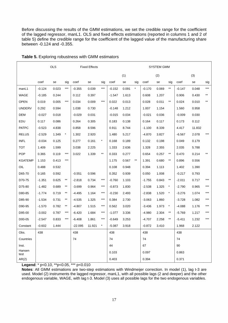
Table 5 documents different system GMM estimations. In columns 3 and 4 of table 5, we report the estimation results adopting the first of the solutions offered by Roodman. In column 3, lag 3 (manL1t-3 and WAGE t-3) are used. In column 4, the lagged value of manufacturing which is the most troublesome variable as it is the one responsible for the “dynamic panel bias” is instrumented with all possible lags (two and deeper), while WAGE, which is the other endogenous variable in our analysis, is instrumented with lag 3. In the last column of table 5 we use with all possible lags for the two endogenous variables.

17

Before discussing the results of the GMM estimations, we set the credible range for the coefficient of the lagged regressor, manL1. OLS and fixed effects estimations (reported in columns 1 and 2 of table 5) define the credible range for the coefficient of the lagged value of the manufacturing share between -0.124 and -0.355.

Table 5. Exploring robustness with GMM estimators

OLS Fixed Effects

SYSTEM GMM

(1) (2) (3)

coef se sig coef se sig coef se sig coef se sig coef se sig

manL1 -0.124 0.023 *** -0.355 0.039 *** -0.152 0.091 * -0.170 0.069 ** -0.147 0.048 ***

WAGE -0.185 0.244 0.112 0.397 -1.547 1.613 0.608 1.207 0.906 0.430 **

OPEN 0.019 0.005 *** 0.034 0.009 *** 0.022 0.013 0.028 0.011 ** 0.024 0.010 **

UNDERV 0.292 0.594 1.038 0.730 -0.148 1.212 1.007 1.154 1.560 0.958

DEM -0.027 0.018 -0.029 0.031 -0.015 0.034 -0.021 0.036 -0.009 0.030

EDU 0.117 0.086 0.264 0.305 0.183 0.138 0.164 0.117 0.173 0.112

PATPC -0.523 4.838 0.858 8.596 0.911 8.744 -1.100 8.339 4.417 11.832

RELUS -2.529 1.349 * 1.302 2.920 1.480 5.217 -4.870 3.827 -6.567 2.078 ***

INFL -0.034 0.125 0.277 0.161 * 0.168 0.189 0.132 0.198 0.049 0.179

TOT 1.409 1.599 3.038 2.225 1.333 2.636 1.328 2.355 2.035 5.788

POP 0.365 0.119 *** 3.022 1.339 ** 0.333 0.277 0.654 0.257 ** 0.470 0.214 **

KGATEMP 1.153 0.413 *** 1.175 0.567 ** 1.391 0.680 ** 0.896 0.556

OIL 0.488 0.532 0.108 0.948 0.394 1.113 1.402 1.390

D65-70 0.165 0.592 -0.551 0.596 0.352 0.939 0.050 1.008 -0.217 0.793

D70-75 -1.351 0.625 ** -2.818 0.734 *** -0.760 1.103 -1.755 0.843 ** -2.011 0.717 ***

D75-80 -1.482 0.689 ** -3.699 0.964 *** -0.873 1.830 -2.538 1.325 * -2.790 0.965 ***

D80-85 -1.774 0.719 ** -4.495 1.164 *** -0.230 2.493 -2.838 1.520 * -3.276 1.074 ***

D85-90 -1.534 0.731 ** -4.535 1.325 *** 0.384 2.730 -3.063 1.860 -3.728 1.082 ***

D90-95 -1.570 0.782 ** -4.807 1.515 *** 0.562 3.020 -3.436 1.973 * -4.088 1.176 ***

D95-00 -3.002 0.787 *** -6.420 1.684 *** -1.077 3.336 -4.980 2.304 ** -5.769 1.217 ***

D00-05 -2.547 0.833 *** -6.408 1.861 *** -0.649 3.253 -4.707 2.258 ** -5.411 1.232 ***

Constant -0.602 1.444 -22.095 11.921 * -5.087 3.918 -0.872 3.410 1.968 2.122

Obs. 438 438 438 438 438

Countries 74 74 74 74

Inst. 44 67 90 Hansen test 0.103 0.097 0.863

AR(2) 0.403 0.394 0.371

Legend: * p<0.10, **p<0.05, *** p<0.010 Notes: All GMM estimations are two-step estimations with Windmeijer correction. In model (1), lag t-3 are used. Model (2) instruments the lagged regressor, manL1, with all possible lags (2 and deeper) and the other endogenous variable, WAGE, with lag t-3. Model (3) uses all possible lags for the two endogenous variables.

18

In the case of system GMM with lags 3 (model 1), the p-value of the Hansen test is 0.103, which means that the null hypothesis of exogeneity of the instruments is not rejected. The coefficient on lagged manufacturing is significant as in all previous estimations and falls within the credible range. Nevertheless, results on the other explanatory variables do not fully confirm previous estimations.

When the set of instruments increases and includes lags 2 and deeper for the lagged value of manufacturing and lags 3 for WAGE (model 2), the p-value of the Hansen test goes slightly below 0.1 but not enough to reject the null hypothesis. The coefficient on the lagged value of manufacturing is significant and credible and the rest of the results are by and large robust.

When all available lags are allowed in the model, the number of instruments is higher than the number of groups and the Hansen test shows clear symptoms of instruments proliferation. However, the lagged value of manufacturing is significant and still within the credible range. Openness, inflation, wages, population and RELUS are significant and signs are consistent with expectations and previous estimations.

Given the criteria mentioned above, it seems that model (2) would be our preferred model. Here the effect of lagged manufacturing is lower than in Hausman and Taylor estimations and undervaluation looses significance. Still, expectations on the signs of the variables are by and large verified.

6.2 Mixed linear models

Do mixed linear models confirm or add on to our results? Mixed linear models permit random parameter variation to depend on observable variables, i.e. allow explanatory variables to have a different effect for each country. Among all the variants of mixed models, we apply a random slopes model in which not only the intercept (as in a random effect model) but also the coefficients of some variables are allowed to change across countries.

We estimated random slopes models allowing one single variable at a time to have a random coefficient. We repeated this procedure for each single explanatory variable. In the first instance, we did not impose restrictions on the correlation of the random effects, i.e. we did not assume that the random effects are uncorrelated with each other. If the model failed to converge, we assumed uncorrelated random effects. After each estimation, we checked the p-value of the LR test and retained only the models for which the null hypothesis was rejected, i.e. random slopes do add information to the random intercept model.

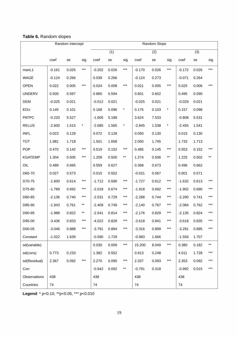
Results show that adding random slopes for all variables, but openness, USPTO patents per capita and the size of the population does not add information. In table 6 we report results of a random intercept model (this is equivalent to a random effect model and is included here for comparison to the other models) and three random slope models where OPEN, PATPC, and POP respectively are allowed to have random slopes. Note that a model where these three random slopes are contemporaneously introduced fails to converge.

19

Table 6. Random slopes Random Intercept Random Slope

(1) (2) (3)

coef se sig coef se sig coef se sig coef se sig

manL1 -0.161 0.025 *** -0.202 0.026 *** -0.170 0.026 *** -0.172 0.026 ***

WAGE -0.124 0.266 0.039 0.266 -0.124 0.273 -0.071 0.264

OPEN 0.022 0.005 *** 0.024 0.008 *** 0.021 0.005 *** 0.025 0.006 ***

UNDERV 0.500 0.597 0.860 0.594 0.601 0.602 0.495 0.590

DEM -0.025 0.021 -0.012 0.021 -0.025 0.021 -0.029 0.021

EDU 0.145 0.101 0.168 0.096 * 0.175 0.103 * 0.157 0.098

PATPC -0.220 5.527 -1.605 5.188 3.624 7.533 -0.808 5.531

RELUS -2.600 1.515 * -2.685 1.565 * -2.845 1.538 * -2.455 1.541

INFL 0.023 0.129 0.072 0.128 0.050 0.130 0.015 0.130

TOT 1.981 1.718 1.501 1.658 2.050 1.745 1.733 1.713

POP 0.470 0.142 *** 0.519 0.152 *** 0.485 0.145 *** 0.553 0.152 ***

KGATEMP 1.304 0.505 *** 1.209 0.500 ** 1.274 0.506 ** 1.225 0.502 **

OIL 0.489 0.665 0.559 0.627 0.368 0.673 0.496 0.662

D65-70 0.027 0.573 0.015 0.552 -0.021 0.567 0.001 0.571

D70-75 -1.600 0.614 *** -1.712 0.590 *** -1.727 0.612 *** -1.632 0.613 ***

D75-80 -1.789 0.692 *** -2.018 0.674 *** -1.918 0.692 *** -1.902 0.690 ***

D80-85 -2.136 0.740 *** -2.531 0.729 *** -2.288 0.744 *** -2.290 0.741 ***

D85-90 -1.943 0.761 ** -2.409 0.749 *** -2.140 0.767 *** -2.084 0.762 ***

D90-95 -1.988 0.822 ** -2.541 0.814 *** -2.176 0.829 *** -2.135 0.824 ***

D95-00 -3.436 0.833 *** -4.022 0.828 *** -3.618 0.841 *** -3.618 0.835 ***

D00-05 -3.046 0.888 *** -3.791 0.894 *** -3.316 0.899 *** -3.291 0.895 ***

Constant -1.022 1.639 -0.590 1.729 -0.983 1.666 -1.556 1.707

sd(variable) 0.030 0.009 *** 15.200 8.049 *** 0.380 0.182 **

sd(cons) 0.773 0.233 1.382 0.552 0.913 0.248 4.011 1.728 ***

sd(Residual) 2.367 0.092 *** 2.270 0.095 *** 2.337 0.093 *** 2.353 0.092 ***

Corr -0.942 0.092 ** -0.791 0.318 -0.992 0.015 ***

Observations 438 438 438 438

Countries 74 74 74 74

Legend: * p<0.10, **p<0.05, *** p<0.010

20

When OPEN, PATPC, and POP are allowed to have random slopes, previous findings are confirmed. The standard deviations of these variables are always significant and parameter estimates are pretty robust across the four specifications. Interestingly, in models (1) and (2), the coefficients on education and RELUS become significant and have the expected sign.

6.3 Alternative measures of institutions

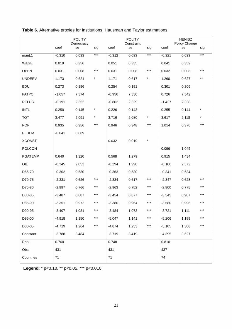
In order to check whether the results on institutions depend on the selected measure, we experiment three alternative indicators. The first two come from the Polity IV dataset (Marshall and Jaggers, 2002) and are the democracy index (P_DEM) and the measure of constraint on the executive (XCONST), which is one of the components of the democracy index. The third, POLCON, is an index of political credibility developed by Henisz (2000, 2002). This index measures the feasibility of policy change, i.e. the extent to which a change in the preferences of any one political actor may lead to a change in government policy. It goes from 0 to 1, with higher scores associated with less feasibility of policy change.

As in previous estimations, the exogeneity of these variables is checked by means of Hausman tests. The Polity measure of democracy, P_DEM, is the only exogenous variable.

Estimations results are reported in table 6 and confirm that democracy is negatively and not significantly linked to industrialization. Yet, indicators that capture decision making processes are positively associated to industrialization and the Polity indicator of constraint on the executive is even significant. These results seem to confirm that what matters is not democracy per se, but rather the presence of functioning decision rules.

21

Table 6. Alternative proxies for institutions, Hausman and Taylor estimations

POLITY Democracy

POLITY Constraint

HENISZ Policy Change

coef se sig coef se sig coef se sig

manL1 -0.310 0.033 *** -0.312 0.033 *** -0.321 0.033 ***

WAGE 0.019 0.356 0.051 0.355 0.041 0.359

OPEN 0.031 0.008 *** 0.031 0.008 *** 0.032 0.008 ***

UNDERV 1.173 0.621 * 1.171 0.617 * 1.260 0.627 **

EDU 0.273 0.196 0.254 0.191 0.301 0.206

PATPC -1.657 7.374 -0.956 7.330 0.726 7.542

RELUS -0.191 2.352 -0.802 2.329 -1.427 2.338

INFL 0.250 0.145 * 0.226 0.143 0.255 0.144 *

TOT 3.477 2.091 * 3.716 2.080 * 3.617 2.118 *

POP 0.935 0.356 *** 0.946 0.348 *** 1.014 0.370 ***

P_DEM -0.041 0.069

XCONST 0.032 0.019 *

POLCON 0.096 1.045

KGATEMP 0.640 1.320 0.568 1.279 0.915 1.434

OIL -0.345 2.053 -0.294 1.990 -0.186 2.372

D65-70 -0.302 0.530 -0.363 0.530 -0.341 0.534

D70-75 -2.331 0.626 *** -2.334 0.617 *** -2.347 0.628 ***

D75-80 -2.997 0.766 *** -2.963 0.752 *** -2.900 0.775 ***

D80-85 -3.487 0.887 *** -3.454 0.877 *** -3.545 0.907 ***

D85-90 -3.351 0.972 *** -3.380 0.964 *** -3.580 0.996 ***

D90-95 -3.407 1.081 *** -3.484 1.073 *** -3.721 1.111 ***

D95-00 -4.918 1.150 *** -5.047 1.141 *** -5.206 1.189 ***

D00-05 -4.719 1.264 *** -4.874 1.253 *** -5.105 1.308 ***

Constant -3.788 3.484 -3.719 3.419 -4.395 3.627

Rho 0.760 0.748 0.810

Obs 431 431 437

Countries 71 71 74

Legend: * p<0.10, ** p<0.05, *** p<0.010

22

7 CONCLUSIONS Since early theories in economic development, manufacturing has been viewed as a special sector capable of spurring economic growth. Cornwall (1977) formulated a model to explain the role of growth of manufacturing output for GDP growth. Two main equations constitute this model: the first explains the growth in manufacturing output, the second the growth of GDP as dependent on the growth of manufacturing output. Later studies estimated the reduced form of this model and so analysed the impact of industrialization and some other explanatory variables on growth. The present paper aimed at contributing to this strand of literature by exploring the determinants of industrialization in a sample of 74 countries from 1960 to 2005. In order to do so, it looks directly at the first equation of the Cornwall model, i.e. the one explaining the growth of the manufacturing output, before it feeds into the equation of economic growth. In this way, it investigates why some countries industrialized and some others did not. If industrialization is a crucial step towards development, this study becomes relevant for the economic and political debate on growth and development.

A measure of industrialization, the first difference of the share of manufacturing in GDP, was regressed over a set of variables that existing literature identifies as factors behind industrialization. Results show that industrialization is faster for larger countries with an undeveloped industrial base and development strategies based on trade openness, undervaluation, skills and knowledge accumulation.

Trade openness positively affects the expansion of the manufacturing sector. This result found only mild support in previous empirical studies (among others, Fagerberg and Verspagen, 1999, 2007; Rodrik et al., 2004; Fagerberg and Schrolec, 2008; Szirmai and Verspagen, 2011) and so seems to suggest that trade stimulates the expansion of the manufacturing sector, instead of affecting directly economic growth. According to our findings, price competitiveness is only partly supported as a driver of industrialization. Exchange rate undervaluation matters but wages do not. On the one hand, Rodrik (2008) provided evidence for undervaluation as a successful factor for industrialization. On the other hand, that labour costs do not constitute factors of competitiveness is consistent with the Schumpeterian view of competitiveness based on innovation rather than costs.7 Inflation is positively and significantly related to industrialization and this contradicts the theories according to which growth and industrialization strictly require low inflation. Finally, institutions, as reflected in democracy indexes, are not determinants of industrializations but an indicator of constraint on the executive is positively and significantly associated to our measure of industrialization. These results confirm previous findings about the modest impact of democratic political systems on growth in developing countries (Fagerberg and Schrolec, 2008).

Studies of the evolutionary approach to innovation and development claim that catching up demands the acquisition of technological capabilities (see the experiences of Korea and the other Asian NICs). Nevertheless, empirical work on manufacturing and growth has seldom looked at the role of R&D expenditures and patents. This paper shows that technical change matters for industrialization. In particular, innovation measured by R&D expenditures, patents granted by national patent offices and an indicator of technological level based on USPTO patents and R&D expenditures is positively and significantly related to industrialization.

Our analysis also demonstrates that industrializing has become more difficult over time. An investigation of the evolution of the determinants of industrialization over different sub-periods evidences that underdeveloped manufacturing bases, trade openness, and the size of the domestic market are constant determinant of industrialization throughout the whole panel. Undervaluation and technological backwardness, instead, mattered only in the period from 1970 to

7 This hypothesis was empirically verified by Fagerberg (1988) and Fagerberg et al. (2007).

23

1995, while absorptive capacity and technological capabilities, as measured by R&D expenditures and technological level, became critical only after 1995.

Extant literature has found a similar pattern for GDP growth and has explained it with the decreasing role of imitation and diffusion and the greater requirements in terms of skills and technological capabilities that characterize modern capitalism (Fagerberg and Verspagen, 1999, 2002, 2007). Our results confirm these findings and show that these patterns are not only relevant for GDP growth but also to manufacturing growth. This has potentially important implications as to how we perceive the manufacturing sector and how we gauge the hypothesis of manufacturing as an engine of growth in modern times.

Acknowledging that innovation has a systemic nature, we inquired into the role of innovation depends upon the interplay of different factors, such as the trade-orientation of the country or other macroeconomic factors such as inflation and undervaluation. Against expectations, none of these interactions terms turned out to be significant. One direction for future research is to find other methodologies to test for policy interdependencies that are likely to play an important role, despite the results of our econometric analysis.

This study is limited by data availability, especially with respect to wages and institutions. For the first variable, it would be useful to find reliable data sources to fill the gaps in the UNIDO dataset. For the second variable, it would be interesting to go beyond democracy indexes and explore more “governance-related” institutional variables. Different dependent variables, like labour productivity, could also be tested.

Future research can also analyse the role of innovation by disaggregating the share of manufacturing into sectoral shares. In this way, it becomes possible to investigate the determinants of structural change towards more knowledge intensive manufacturing sectors. Connected to this point it is the role of manufacturing as an engine of growth. Which types of industrialization strategies (also in terms of sector targets) are more conducive to economic growth? And which of these strategies can guarantee sustained economic growth over time?

24

References

Abramovitz, M. (1986), Catching up, Forging ahead, and Falling behind, Journal of Economic History, 46: 386-406.

Acemoglu, D., Johnson, S., Robinson, J. A. (2001), The Colonial Origins of Comparative Development: An Empirical Investigation, The American Economic Review, 91(5): 1369-1401.

Amable, B., and Verspagen, B. (1995), The Role of Technology in Market Shares Dynamics, Applied Economics, 27: 197-204.

Amendola, G., Dosi, G., and Papagni, E. (1993), The Dynamics of International Competitiveness, Review of World Dynamics, 193(3): 451-471.

Baltagi, B., Brensson, G. and Pirotte, A. (2003), Fixed Effects, random effects or Hausman-Taylor? A pretest estimator, Economics Letters, 79(3), 361-369.

Castellacci F., and Natera, J. M. (2011), A new panel dataset for cross-country analyses of national systems, growth and development (CANA), Innovation and Development, 1(2).

Chenery, H., Robinson, S., and Syrquin, M., 1986. Industrialization and Growth. A Comparative Study, New York: Oxford University Press.

Cimoli, M., and Katz, J. (2003), Structural reforms, technological gaps and economic development: a Latin American perspective, Industrial and Corporate Change, 12(2): 387-411.

Cohen, W. and Levinthal, D. (1990), Absorptive capacity: A new perspective on learning and innovation, Administrative Science Quarterly, 35(1): 128-152.

Cornwall, J., 1977, Modern Capitalism. Its Growth and Transformation, New York: St. Martin's Press.

Dollar, D., and Kraay, A. (2003), Institutions, Trade, and Growth, Journal of Monetary Economics,50: 133–162.

Fagerberg J. (1988), International competitiveness, Economic Journal, 98: 355-74.

Fagerberg, J. and B. Verspagen (1999). ‘Modern Capitalism in the 1970s and 1980s’, in M. Setterfield ed., Growth, Employment and Inflation, Houndmills, Basingstoke, MacMillan.

Fagerberg, J., and Verspagen, B. (2002), Technology-gaps, Innovation-diffusion and Transformation: an Evolutionary Interpretation, Research Policy, 31: 1291-1304.

Fagerberg, J., Srholec, M., & Knell, M. (2007). The Competitiveness of Nations: Why Some Countries Prosper While Others Fall Behind, World Development, 35(10), 1595-1620.

Fagerberg, J., and Srholec, M. (2008), National innovation systems, capabilities and economic development, Research Policy, 37: 1417–1435.

Fagerberg, J., Shrolec, M., and Verspagen, B. (2010), “Innovation and Development”, in B. Hall and N. Rosenberg (eds), Handbook of the Economics of Innovation, Elsevier: North Holland, pp. 833-872.

Fei J.C., and Ranis G. (1964) Development of the labour surplus economy. Irwin, Homewood.

Freeman, C. 1987. Technology Policy and Economic Performance: Lessons from Japan, London, Frances Pinter.

Gerschenkron, A. (1962), Economic Backwardness in Historical Perspective, Cambridge MA: Harvard University Press.

Haan, J. (2007), Political institutions and economic growth reconsidered, Public Choice (131): 281–29.

25

Hausman, J. A. and W. E. Taylor (1981). ’Panel Data and Unobservable Individual Effects’, Econometrica, 49(6): 1377-98.

Henisz, W. J. (2000), The Institutional Environment for Economic Growth, Economics and Politics, 12(1): 1-31.

Henisz, W. J. (2002), The Institutional Environment for Infrastructure Investment, Industrial and Corporate Change, 11(2): 355-389.

Heston, A., Summers, R., and Aten, B. (2009), Penn world table version 7.0, Center for International Comparisons of Production, Income and Prices at the University of Pennsylvania.

Kaldor, N. 1967, Strategic Factors in Economic Development, Ithaca: Cornell University.

Kaldor, N. (1978), The Effects of Devaluation on Trade in Manufactures, in Future Essays on Applied Economics, Duckworth, London.

Katuria, V., and Raj, R.S.N. (2009), Is Manufacturing an Engine of Growth in India? Analyis in the Post Nineties, Paper for the UNU-WIDER/UNU-MERIT/UNIDO.

Kim, L. (1980), Technology Policy for Industrialization: A Model, Research Policy, 9: 254-277.

Kosakoff, B., and Ramos, A. H. (2009), “Macroeconomic Evolution in High Uncertainty Contexts: The Manufacturing Sector in Argentina”, in M. Cimoli, G. Dosi, and J. E. Stiglitz (eds), Industrial Policy and Devleopment. The Political Economy of Capabilities Accumulation, New York: Oxford University Press, pp. 239-256.

Kuznets, S. (1973), Modern Economic Growth: Findings and Reflections, The American Economic Review, 63(3): 247-258.

Lall, S. (1992), Technological capabilities and industrialization, World Development, 20(2): 165-186.

Lederman, D. and Saenz, L. (2005), Innovation and development around the world, 1960-2000.

Lee, K., and Kim, B. (2009), Both Institutions and Policies Matter but Differently for Different Income Groups of Countries: Determinants of Long-Run Economic Growth Revisited, World Development, 37(3): 533-549.

Lewis, W.A. (1954), Economic development with unlimited supply of labor, Manchester School of Economic and Social Studies, 22: 139-191.

Lundvall, B.-A. (ed.) 1992. National Systems of Innovation: Towards a Theory of Innovation and Interactive Learning, London, Pinter.

Jacob, J. and T. Osang (2007). Institutions, Geography and Trade: A Panel Data Study, Departmental Working Papers 0706, Southern Methodist University, Department of Economics.

Marshall, M. G., and Jaggers., K., (2002) “Polity IV Dataset,” [Computer file; version p4v2001] College Park, MD: Center for International Development and Conflict Management, University of Maryland.

Nelson, R. (1993), National Innovation Systems. A Comparative Analysis, New York: Oxford University Press.

Nelson, R.R., and Pack, H. (1999), The Asian Miracle and Modern Growth Theory’, Economic Journal, 109: 416-436.

Nelson, R.R., and Sampat, B.N. (2001), Making sense of institutions as a factor shaping economic performance, Journal of Economic Behavior and Organization, 44: 31-54.

Prebisch, R., (1950), The Economic Development of Latin America and its Principal Problems, New York, United Nations. Reprinted in Economic Bulletin for Latin America, 7(1):1-22.

26

Rodrik, D. (2008), The Real Exchange Rate and Economic Growth, Brookings Papers on Economic Activity, Fall 2008, pp. 365-412.

Rodrik, D., Subramanian, A., and Trebbi, F. (2004), Institutions Rule: The Primacy of Institutions Over Geography and Integration in Economic Development, Journal of Economic Growth, 9(2), 131-165.

Roodman, D. (2006). How to Do xtabond2: An Introduction to "Difference" and "System" GMM in Stata, Center for Global Development Working Paper No. 103.

Roodman, D. (2009). A Note on the Theme of Too Many Instruments, Oxford Bulletin of Economics and Statistics, 71(1).

Singer, H. (1950), The Distribution of Gains between Investing and Borrowing Countries, American Economic Review, 40: 473-485.

Solow, R. (1957), Technical Change and the Aggregate Production Function, The Review of Economics and Statistics, 39(3): 312-320.

Szirmai, A. (2009). Industrialisation as an Engine of Growth in Developing Countries, 1950-2005, UNU-MERIT working paper, 2009-10.

Szirmai, A. (2011): “Industrialisation as an engine of growth in developing countries, 1950– 2005”, Structural Change and Economic Dynamics (06 February 2011).

Szimai and Verspagen (2011), Manufacturing and Economic Growth in Developing Countries, 1950-2005, UNU-MERIT Working Paper 2011-069.

Timmer, M. P., and de Vries, G.J. (2009), Structural Change and Growth Accelerations in Asia and Latin America: A New Sectoral Dataset, Cliometrica, 3(2): 165-190.

Tregenna, F. (2007), Which Sectors Can be Engines of Growth and Employment in South Africa?: An Analysis of Manufacturing and Services, Paper presented at the UNU-WIDER CIBS Conference.

Vanhanen, T. (2000), A New Dataset for Measuring Democracy, 1810-1998, Journal of Peace Research, 37(2): 251-265.

Veblen, T. (1915), Imperial Germany and the Industrial Revolution. New York: Macmilllan.