the determinants of australian investments abroad
TRANSCRIPT

The Determinants of Australian Investments Abroad
ERASMUS UNIVERSITY ROTTERDAM
Erasmus school of Economics
Department of Economics
Supervisor: Prof. dr. Giovanni Facchini Name: Mattia Mariani Exam number: 322565 Email address: [email protected] Key-words: Determinants of FDI, Australia, panel data, OLS analysis.

2
dedicated to my beloved grandad and my dog
3
INDEX
INDEX ..................................................................................................................... 3
1. INTRODUCTION ............................................................................................ 4
2. LITERATURE REVIEW ................................................................................ 7
2.1 Theoretical background ................................................................................. 7
2.1.1 FDI analysis models................................................................................. 7
2.1.2 Types of FDI ............................................................................................10
2.2 Determinants of FDI ......................................................................................11
2.2.1 Traditional Variables ..............................................................................12
2.2.2 Non-traditional variables .......................................................................18
3. OVERVIEW ON AUSTRALIAN FDI ........................................................ 22
3.1 Historical background...................................................................................22
3.2 Australian FDI – data and statistics ..............................................................24
4. METHODOLOGY ......................................................................................... 29
4.1 Variables selection process...........................................................................29
4.2 Estimation method ........................................................................................30
4.2.1 Econometric models ...............................................................................30
4.2.2 The extreme bounds analysis ................................................................31
5. VARIABLES................................................................................................... 34
5.1 Endogenous variable.....................................................................................34
5.2 Exogenous variables .....................................................................................35
5.2.1 Variables included in the analysis .........................................................35
5.2.2 Variables excluded from the models .....................................................39
6. EMPIRICAL ANALYSIS .............................................................................. 40
6.1 Australian direct investment abroad – general model.................................41
6.1.1 OLS and Fixed Effects estimation method .............................................41
6.1.2 Extreme bounds analysis .......................................................................45
6.2 Australian direct investment abroad – robustness check for wage variable .............................................................................................................................46
7. CONCLUSIONS ............................................................................................. 49
REFERENCES .................................................................................................... 51
ACKNOWLEDGEMENTS ............................................................................... 62
APPENDIX A ..................................................................................................... 63
APPENDIX B ..................................................................................................... 66

4
CHAPTER ONE
1. INTRODUCTION
Australia is a very interesting country, thanks to its geographical proximity to
Asia and its cultural links with Europe and the Western world.
According to CIA (2009)1 in terms of its GDP per capita, expressed in purchasing
power parity, it ranks 26th in the World, above some leading economies like
France, the UK and Germany. Moreover, Australia has seen its importance
increase both as a destination and as a source of foreign direct investments
(from now on called FDI). It is now ranked 14th in both2.
The Australian experience can be considered, according to Rafferty and Bryan
(1998), an “extreme case of FDI growth”3 with a spectacular increase from the
second half of the 1980s, faster than the rest of the world as a whole followed by
a rapid contraction between 1988 and 1991 and a second burst of growth from
1992 to the present days. After the Second World War the increasing importance
of the phenomenon of FDI seems to be exceeded only by the huge amount of
researches about this topic, as it has been pointed out among others by Agarwal
(1980). However, the amount of research which has studied outward FDI is
relatively small if compared to the amount of work which has focused on inward
FDI. Furthermore, looking at the Australian case, it seems that the difference
between the two aspects is even greater. This could derive by the fact that
inward FDI flows have been for a long time far greater than outwards flows and
1 See CIA The World Factbook https://www.cia.gov/library/publications/the-world-
factbook/rankorder/2004rank.html?countryName=Australia&countryCode=AS®ionCode=au
#AS
2 See CIA The World Factbook https://www.cia.gov/library/publications/the-world-
factbook/rankorder/2199rank.html?countryName=Australia&countryCode=AS®ionCode=au
#AS
3 See Rafferty & Bryan (1998), p.3.

5
the importance of Australian investments abroad has grown only in more recent
years.
This research aims at explaining the most important determinants of Australian
FDI abroad, focusing on macroeconomics variables that can push Australian
firms to prefer direct investment instead of simple trade with a foreign country.
Several variables, taken from previous literature and combined in an original
way, are used to model the flows, and different econometric techniques are
implemented to identify the most robust determinants. The approach takes into
account the evolution of the significance of the variables both across countries
and time. All the econometric results are linked to the existing theoretical
frameworks found in the literature, and in particular to the OLI model
(Ownership, Location and Internalization) introduced by Dunning (1977, 2000)4;
the OLI model has been deeply studied and commonly applied in the past5 so it is
a very useful benchmark for other studies focusing on the drivers of FDI.
The study focuses on the second surge of FDI, and thus our data cover the period
from 1992 until 2007. The purpose is to improve the literature making a
substantial contribution to the topic of FDI outwards, both in a general context
and in a specific one, Australia in our case.
This paper is organized as follows. Chapter Two is divided in two main parts: the
first is entirely devoted to provide a theoretical framework in order to
comprehend in a better and wider way the reasons that could make a firm opt for
a direct investment in a foreign country. It provides a brief description of the
various models that have dealt with market entry decisions, especially focusing
on the OLI model. The second part reviews the literature on the determinants of
outwards FDI; in particular, we discuss in detail previous studies, which have
used the same controls we have employed in this research. Chapter three
provides a brief historical overview on Australian FDI and multinational activity,
4 Dunning introduced the OLI model in 1977 in a Nobel Symposium in Stockholm; the model has
been updated in the following years by the author himself.
5 See Zhao & Decker (2004), p. 8.

6
focusing on the sectors where investments are prominent; a comparison
between major trading partners and investment recipients is also done to better
understand the reasons behind the different choices of market entry. Chapter
Four explains the methodology followed in the paper, provides detailed
information on the econometric approach implemented and illustrates the
variables selection process; Chapter Five describes the variables utilized in the
research, especially paying attention on how they are defined and constructed.
The regression results, with all the related interpretations, are presented in
section six. The last chapter includes concluding remarks.

7
CHAPTER TWO
2. LITERATURE REVIEW
The literature dealing with FDI can be classified in two main branches, as pointed
out by Agiomirgianakis, Asteriou and Papathoma (2003): the first explains the
effect of FDI on the process of economic growth while the second one goes deep
through the study of the determinants of the FDI. In this work we are not
concerned with the link between FDI and growth, and as a result, we focus on the
second strand of literature and it try to summarize how it answers the following
question: why would a firm -- in our case an Australian one -- want to locate its
production in a foreign country?
2.1 Theoretical background
2.1.1 FDI analysis models
Many authors have tried to find a reasonable answer to this question. One of the
earliest works dealing with that is a pioneering contribution of Mundell (1957):
his approach focuses on the relative endowments and costs of factor of
production. Its conclusions suggest that capital flows are positively correlated
with big differences between capital-rich and capital-poor country; also high
barriers to trade and migration are found as factors that facilitate FDI. Obviously
these determinants are not sufficient to explain all the reasons of direct
investments. A general theory of direct investments abroad can be found in the
so-called OLI theory. John Dunning introduces his “Eclectic Paradigm” (1977)

8
and asserts that firms choose FDI market entry to obtain three different
advantages6:
ownership advantages
location advantages
internalization advantages
The first ones derive from specific assets, tangible or intangible, owned by the
firm and that grant an advantage over the other enterprises; ownership
advantages permit the firm to afford the cost brought by foreign environment
(for example the costs of dealing with foreign administrations and regulatory
framework) and to compete with local firms. Internalization advantages could
come from retaining control over the firm-specific assets7, instead of licensing to
firms already based in the foreign country. Location advantages make it more
profitable to invest in a country instead of only trading with it, if the firm uses
some inputs located abroad. The OLI model has been supported by several
empirical studies and this is really important, as it permits to use it as a
benchmark for comparison and to give a strong theoretical background to our
work. For example8, the ideas from the OLI model have been applied by
Deichmann (2004) in explaining FDI in Poland and by Nakos and Brouthers
(2002) in a study about entry market decisions in Central and Eastern European
countries. The limitations of the model lie in the fact that in the attempt to
explore all the factors determining the entry mode it “ignores the impact of the
firm objective, the decision maker, and the situational contingency surrounding
the decision maker when the entry mode decision choice is made” (Zhao &
6 The 1977 work has been extended in further studies by Dunning with the introduction of other
characteristics that have to be considered in the market entry decision, like competition
advantages, market failure, dynamic environment and collaboration.
7 For firm-specific assets are intended the quality of a brand name, managerial skills or process
that provide an advantage to the firm over the others; licensing them would diminish this
advantage.
8 In the literature there are other several examples of empirical studies on the OLI like Agarwal
and Ramaswami (1992) and Tarzi (2005).

9
Decker, 2004)9. To better understand the decision of MNEs of becoming
international, extensions of the OLI model can be found in the more recent
literature: Guisinger (2001), for example, develops an “evolved eclectic
paradigm” also called OLMA model. In this case the “M” stands for a group of
factors representing the mode of entry; the “A” represents, on the other hand, the
adaptation that the firm has to carry out when it has to deal with the business
environment of the foreign country where the investment takes place10.
The OLI theoretical framework, with its extensions, is not the only model that
tries to capture the determinants of different market entry decisions; in their
already cited paper, Zhao and Decker (2004), in fact, end up in finding five
different models that take into account different determinants11. The “stage of
development” (SD) model, which was proposed by Johanson and Paul (1975),
considers the internalization plans of multinationals as a process depending on
the stage of a firm’s development. Another model identified is called OC and it
takes into account the organizational capacity of a firm in the choice of market
entry: the firm will chose to become international if this decision is supported by
a possibility of future development and deployment of the firm’s capabilities12.
Differently, Anderson and Gautignon (1986) assert that a firm wants, as a
primary goal, to maximize the overall efficiency of the production process by
minimizing the transaction costs. For this reason their model is known as
Transaction Costs Analysis (TCA); like for the OLI model, there are a lot of
studies on the TCA model and it can count on a lot of theoretical extensions and
support. On the other hand, these works have shown the weakness of the model:
the two most important of these weak points is surely the fact that the
9 See p.27.
10 In his explanation of this modified OLI model, Guisinger also investigates the differences
between domestic and foreign investment in order to capture the peculiar characteristics of FDI.
11 The OLI model is included and studied with these five different models. For a quick comparison
between them see table 1, p. 27. Since most of the previous studies about FDI relate to the OLI
model and since this work focuses mainly on the location determinants, the other models are
only briefly described.
12 The model was introduced by Aulakh and Kotabe (1997) and developed by Madhok (1998).
For further information see these two studies.

10
transaction costs of a firm are really hard to measure and that there is no clear
relationship between them and the firm’s corporate governance. The last model
that Zhao and Decker (2004) specify is the so-called DMP13 model: in this case
the market entry decision is seen as a decision making process consisting of
different stages that consider several factors as costs, risk, existing business
environments and so on. The model has been sistematically studied and
empirically tested (Kumar and Subramaniam, 1997; Pan and Tse, 1999 for
example) and from the empirical studies, it emerged a lack of accuracy in the role
of the decision maker and the organization.
2.1.2 Types of FDI
Now that we have briefly explored the theoretical models we provide an
overview on the different types of FDI which reflect why a firm would want to
become a multinational. Armstrong (2009), considering a view widely accepted
and found in literature, suggests two main reasons: to better serve the local
market and to exploit lower input-costs.
The first choice implies the so-called “horizontal FDI” (also denoted as “market-
seeking”), which aim at developing and building new plants for the production
similar to the one based at home. The motive of these investments is reducing
the costs of supplying the local market, by skipping in some way the transport
costs and the tariffs but especially by the use of cheap labour, often in developing
countries. Horizontal FDI tend to be more attracted by larger host economies
because a big market implies more competition of local firms and a subsequent
product at a lower price. For this reason it is more convenient to invest directly
in the foreign country instead of serving its market through exports which carry
on higher costs. Furthermore, larger markets are characterized by lower plant-
specific fixed cost per unit of output.
13 DMP stand for Decision Making Process and it was proposed by Root in the 1994.

11
The second important reason defines the commonly called “vertical FDI” also
known as “production-cost minimizing” since they are meant to relocate part of
the production chain, either upstream (or backward, towards the source of raw
materials) or downstream (or forward, towards the sale of the final product) in
low cost countries. It is clear that the so-called “raw materials seeking FDI” can
be classified among the vertical FDI: they aim at exploiting the natural resources
of the host country in order to secure a continual supply of raw materials for its
production14. Vertical investments are basically export-oriented to the market of
the investor’s home market so they are not usually affected by the size of the host
economies.
It is interesting to note that horizontal and vertical FDI are both stimulated by
agglomeration (clustering) effects and other two types of FDI are found in
Eitemann, Stonehill and Moffett (1995): “knowledge seeking” investments,
aiming at accessing technology located abroad, and “political safety seeking”,
which are strongly influenced by political risks of the possible location”.
2.2 Determinants of FDI
After having shown the basic theoretical framework, that helps to better
understand the reason of investing, we can turn to the study of the single
determinants used in the analysis and links them to previous empirical
econometric studies.
Surveying the FDI literature, Lim (2001) identifies seven particularly important
factors: as first determinant, found in almost every research, he puts the market
size of the FDI recipient country. Another important determinant is found in the
production factor costs, and economic distance (proxied often by transportation
costs) is also widely recognised as important factor in the market entry choice.
14 These investments are often located in developing countries but there are examples of
developed countries rich in natural resources that are big recipient too; for example, US, Canada
and Australia (Deng, 2003).

12
Between the other factors, the author mentions agglomeration effects, fiscal
incentives, business (investment) climate and moreover trade barriers (or
openness of trade). There are also other determinants which have been found to
play an important role in several existing works15 and we will try to provide a
brief description of the most commonly used. Since our study build a model
using the same variables indicated by Lim (2001) as “traditional variables” and
adding others (“non-traditional”), we follow here the same denomination.
2.2.1 Traditional Variables
Market size
The size of the host country’s local economy is undoubtedly one of the most
commonly used variables in FDI empirical studies; Lim (2001) argues that
horizontal FDI are encouraged by bigger market size, thanks to economies of
scale, and vertical FDI are indifferent16. In several works the market size
determinants is proxied by the GDP of the recipient country and the expected
effect is positive. For example, Shatz and Venables (2000), Padilla and Richards
(1999), Brainard (1997) and Kravis and Lipsey (1982) find a highly positive
correlation between FDI and GDP. For our research, a study by Edwards and
Buckley (1996) on the determinants of FDI from Australia for the 80s and the
first half of the 90s is particularly important: in fact, they have shown that this
factor is among the most important for Australian investments (which are found
to be basically “market seekers” in their study).
Production factor costs
Cost advantages, according to Wezel (2003), are relevant and important
especially for efficiency-seeking FDI. Lim (2001) argues that both vertical and
15 As already explained when discussing about the different types of FDI we could mention
political safety reason or knowledge seeking investments.
16 See section 2.1.2.

13
horizontal FDI are positively affected by a decrease of production factor costs
even if in a different proportion17. An experiment run by Buckley, Devinney and
Louviere (2007), surveying the decision of the managers of firms that face the
decision of investing abroad18, find that almost 50% of the last investments
made, show a tendency towards foreign markets that grant at least a reduction of
production costs of 5%.
Most of the empirical studies analysing the importance of factor of production
costs usually consider labour costs instead of other cost drivers such as capital or
intermediate goods: Wezel (2003), referring to Turner and Golub (1997),
justifies this choice asserting that labour is largely immobile and hence not
affected by price-equalizing effects while the other production factor are.
Furthermore, it is harder to quantify the costs deriving from capital than wage or
unit labour costs19. Also in the choice of proxies for labour costs there are several
different approaches varying from wage (monthly, PPP-adjusted, productivity-
adjusted and so on), unit labour cost, with different definitions20, and GDP per
capita, whenever data limitations make this necessary (for example, Majocchi
and Strange, 2007). However, it seems that the strength of the positive effect on
FDI of labour costs differ from country to country: Feenstra and Hanson (1997),
investigating US FDI in Mexico21, find a highly positive influence. A weaker effect,
but still positive and significant, can be found in the study of Wheeler and Mody
(1992) on US manufacturers worldwide. In another study, by Bevan and Estrin
17 See Lim (2001) p.12. The author asserts that “production cost-minimizing vertical FDI will be
stimulated by lower factor cost. Lower factor cost should also be viewed favourably by horizontal
FDI. The net impact of lower factor cost on FDI is positive”. In section 2.1.2 we also deal with this
topic.
18 The subjects surveyed by the authors are active managers, with both and no experience in FDI
location choice, of firms with headquarters in different countries all over the world. However, the
29% of the sample is headquartered in Australia (Denmark and US are the other two most
represented) so the survey is highly significant for our study.
19 See Lipsey (2002), p.36.
20 See Wezel (2004), p. 12 for some examples of unit labour cost proxy.
21 The authors investigate the case of maquiladoras, American owned plants set in Mexico to take
advantage exactly from lower labour costs.
14
(2004), on the determinants of FDI in Eastern European countries, low labour
costs are found to be the most important factor. On the other hand, Mody,
Dasgupta and Sinha (1999), show that in the case of Japanese FDI in Asia there is
no significant relationship between cheap labour and FDI. In the work of
Edwards and Buckley (1996), useful for a comparison, Australian FDI seems not
to be driven by the desire to exploit cheap labour22.
Economic distance / transport costs
With regard to the role of transportation costs and economic distance between
the investor and the recipient country, the effect is definitely not unambiguous
and depends on the purpose of FDI. In fact, as discussed in Lim (2001),
horizontal FDI are antagonist of trade: if transportation costs are too high, and
hence the access to the foreign market through export is not favourable, the
multinational will tend to produce directly in the host country. So, a greater
distance between the two countries will imply higher transportation costs and a
subsequent increase in horizontal FDI. On the other hand, if we consider vertical
FDI, which require transport costs of components and final products (as shown
in section 2.1.2), it is quite obvious that a great physical distance will affect
negatively the decisions of multinational to invest directly. The final effect of
distance is defined by the prevalence of horizontal or vertical investments, since
they are influenced in an opposite way.
In the literature there are several examples of this ambiguity: in the already cited
study, Brainard (1997) has found a positive relation, suggesting that in this case
the FDI taken into consideration could be more horizontal than vertical23. This
relation is not particularly robust. A very weak relation has in fact been found by
22 However, we must take into consideration that the authors investigate only three recipient
countries: UK, Thailand and Malaysia.
23 The analysis of the author mixes developed countries with developing countries FDI so it is not
possible to identify a specific basic trend that can be taken as “rule” for further studies. Probably,
in this study there is a greater number of multinational that opted for the horizontal investment
than vertical one.

15
Ekholm (1998) exploring Swedish FDI. Furthermore, another study by
Labrianidis on the importance of geographical distance for Greek investments
seems to show a negative relationship: almost all these investments are directed
to neighbouring countries, like Bulgaria, Albania and Romania and, still more
interesting, a within-country analysis shows that the regions closer to Greece are
the biggest recipient. It seems Greek FDI to be heavily affected by geographical
distance so a raise of investments can be expected if transportation costs
decrease24.
Agglomeration effect
The effect of agglomeration on FDI is quite predictable even if there are two
different ways of capturing what agglomeration really is. Some authors focus on
the size of existing FDI stock in a specific place, which makes clustering attractive
while others take into consideration the quality of the infrastructure of the
recipient country.
In the first case, a great cluster of FDI should attract new investments; this is
known as the theory of the “follow-the-leader” effect and it is well explained in
Wezel (2003)25: once a multinational decides to invest in a determined location,
gaining, in this way, competitive advantages as a “first mover”, it puts the other
firms in a position where they should invest as well in the same country to
capture the productivity advantages that would be lost in case of a late
investment. If they don’t do it, or do it too late, they could incur in a big welfare
loss. Furthermore, the best choice for the firms would be to move
simultaneously. Wheeler and Mody (1992) confirm this theory in their empirical
study: they find a highly significant positive relation both for developing and
developed countries. Mody and Srinisvan (1998), bring further evidence showing
the correlation between the amount of past FDI and the present ones.
24 A possible explanation is that Greek FDI in these countries (with very low labour costs) are
merely vertical.
25 See p. 21-22 for a more exhaustive explanation.

16
The second case includes, as a proxy for quality-of-infrastructure, different
examples: Loungani, Mody and Razin (2002) investigate whether telephone
density in developing countries has an effect on attracting FDI. A significant and
positive relationship is found. Khadaroo and Seetanah (2007), studying the FDI
in Sub Saharan Africa, find transport infrastructures to be the most significant
drivers followed by other infrastructure determinants26. Among the first scholars
who dealt with this topic we must mention Root and Ahmed (1979). In all the
cases they consider, the better the infrastructures are, the higher the level of
direct investments.
Fiscal incentives
Fiscal incentives in the recipient country tend to stimulate FDI flows, both of the
horizontal and of the vertical type. Lim (2001) argues though that horizontal FDI
is more affected by other policies that affect the viability of the host markets, like
for example protectionist policies. Fiscal incentives have of course a positive
effect on the cost structure, so cost reducing FDI flows are positively affected. In
fact, a positive effect is found in Woodward and Rolfe (1993). However, it is
important to mention the study of Reuber and others (1973)on the drivers of FDI
both in developed and developing countries: the empirical findings seem not to
be significant and the explanation could be that multinationals expect these
incentives to be only temporary and be followed by a future increase in taxes
because they are totally controlled by the governments of the host country.
Furthermore, Oman (2000) indicates the existence of a two-stage investment
decision process: investors consider at first stage a set of possible locations on
the basis of economic and political factors but here fiscal incentives play no role.
Only when the best locations are chosen that fiscal incentives are taken into
consideration. So, it seems fiscal incentives to play a secondary role.
26 For example communications network is taken into consideration in the analysis.

17
Business climate
Multinationals usually find it more profitable to invest in a friendlier
environment: in fact in such a climate the cost of operating in a foreign country
are lower and so are the risks. With “friendlier” environment we mean similar
regulatory, bureaucratic and judicial climate; both horizontal and vertical FDI
will benefit from less restrictive requirements. In general, countries that share
greater similarities with the investing country are considered better recipients
than countries that show larger differences.
Again, it is not easy to predict a positive or negative relationship and the
empirical work seem to justify this uncertainty; the problem lies in the fact that
different proxies are used to test the theory. Lim (2001) classifies the possible
variables in two categories: economic (like different labour regulations,
performance and technical requirements, difficult enforceability of contracts and
so on) and political risks (among the others, unstable democracies, governments
instability and possible wars). We prefer to analyse political risk as a separate
dimension, in order to capture the peculiarity of this proxy27. For economic
environment proxies, the level of inflation of the host country and the balance of
payments are widely used (Schneider and Frey, 1985). In their study, Edwards
and Buckley (1996) find similar business practice and legal system to be very
important for Australian multinationals.
Openness of trade (trade barriers)
FDI react in an opposite way to an increase in openness (same as a decrease of
trade barriers) depending on their nature: horizontal FDI, which are meant to
skip tariffs on trade, are subject to a decrease while vertical FDI, which imply a
massive flows of goods between the multinational’s home market and the host
economy in the form of trades (as explained in section 2.1.2), will surely benefit
from a more liberal environment. Furthermore, we must take into account that
lower tariffs can improve the quality of the business climate and increase the
27 In this approach we follow for example Wezel (2003), Mody and Srinivasan (1998) and Duncan
(2000).

18
level of FDI. For this reasons, the effect of greater openness of trade on FDI can
not be easily predicted.
Another problem in assessing the effect of trade policies on FDI flows is
represented by the choice of the measure of openness: widely accepted as the
ordinary proxy is the ratio of import or export (in several studies the sum
between the two) to GDP but another possible proxy is also the level of average
tariffs imposed by the host country. More sophisticated indices of openness are
also found in the literature28. The first type can be found in several works like
Dees (1998), Kandiero and Chitiga (2003) and Hausmann and Fernandéz-Arias
(2001) with different results and significance, depending on the nature of FDI
and host countries. Tariff proxy can be found in the already mentioned study by
Brainard (1997).
2.2.2 Non-traditional variables
Now that we have explained the characteristic of the most common determinants
of FDI in this section we give an overview of additional drivers that can help us in
our analysis.
Real Exchange rate
The impact of real exchange rate on FDI it is not clear since there are opposing
views. Kosteletou and Liargovas (2000) an upward movement of the real
exchange rate of the host country can warn foreign firms about a possible future
increase of protectionism and hence encourage further investments in order to
prevent the possible tariff growth29. The opposite effect comes from the relative
28 For example Leamer (1988) builds an index of openness that considers also the deviations
from trade flows while Pritchett (1996) proposes to adjust openness measure with country-
specific determinants like geographic size or per-capita income.
29 See Kosteletou and Liargovas (2000), p. 139. In brief, if the host country real exchange rate
moves upwards, its balance of trade worsens because it is more convenient import from other
countries. For this reason the host country could increase tariffs and level the balance of trade.

19
enrichment of foreign investors when facing a depreciation of the host country’s
currency: the depreciation makes relatively cheaper for foreign firms to buy
assets located in the host country30 (Froot & Stein, 1991) and hence attracts FDI.
As we have seen, an opposite movement of the exchange rate of the host country
can attract FDI and this is why the effect is not easily predictable. Empirically,
Kyiota and Urata (2003) find, studying Japanese and US FDI, that a depreciation
in the currency of the host country positively affects the level of foreign
investments.
Literature shows different results, confirming how difficult it is to find a
significant trend. Another variable which has been often studied is the change of
real exchange rate over time instead of just its level: further attention is paid to
the volatility of exchange rates even if the literature, both theoretical and
empirical, on its impact on FDI is quite limited. Furthermore, there are two
approaches and they seem to reach contradicting conclusions. Brzozowski
(2003) analyses theoretically and empirically both the approaches known as
“production flexibility” and “short-run risk aversion”. The first approach
basically asserts that the effect of exchange rate volatility depend on sunk costs
in capacity, competitive structures and convexity of the profit function in prices.
Since higher expected profits, which attract FDI, are linked with low volatility of
employment and production, a fixed exchange rate system (or however
characterized by low exchange rate volatility) is preferred because it is more
capable to isolate them (employment and production) from monetary shocks31.
The same idea is developed by Darby et al (1999) but in a different way and with
opposite results: both negative and positive relationship is found32. The second
30 For example, let’s say an Australian firm wants to invest in China and has to face an expense of
50 millions yuan (Chinese currency) to buy a plant located there; the firm has one million A$
available. If the exchange rate is 25 yuan/A$ the firm can not buy the plant but if the exchange
rate depreciates till 50 yuan/A$ the investment can take place.
31 See Brzozowski (2003) p. 8-9 and Aizenman (1992).
32 The authors develop a model that takes into account the possibility of waiting instead of
investing now: in this way, waiting time is linked to costs. They find two relationships: the
exchange rate volatility depresses the investment when the expected revenue, the value of

20
approach mainly focuses on risk aversion and suggests that the time lag between
investment and profit in foreign currency plays a fundamental role. Empirically
Brzozowski (2003), studying FDI flows for emerging country, finds a negative
impact of host country’s exchange rate volatility. Differently, Goldberg and
Kolstad (1995) assert that the share of investment abroad unambiguously
increases with high foreign exchange rate volatility.
Country Risk
In this study we decide to deal with country risk separately from business
climate trying to capture its features. However, also among the empirical and
theoretical studies, there are several different factors that have been taken into
account concerning country-specific risks that can discourage investments. The
choice of adding political risk variables to our analysis is justified by the work of
Beyer (2002) and Stevens (2000): the former, using the Economic Freedom
Index33, shows an improvement of his regressions and the latter, investigating
the US investments in Argentina, Brazil and Mexico, sees an increase of the R-
squared for the specifications concerning Argentina. In measuring political risk
we can distinguish between several variables, but often it is measured using
corruption indices, due to the devastating effect that corruption can have on
administrative efficiency. Literature provides proofs of how corruption may
deter direct investment. Smarzynska and Wei (2000) and Everhart and
Sumlinski (2001), for example, find that corruption has a negative effect on FDI.
A limitation of these studies lies in the fact that they do not take into account that
corruption may affect FDI in different ways, depending on the nature of FDI.
Hakkala, Norbäck and Svaleryd (2008), using firm-level data on Swedish
multinationals, try to fill this gap and they find that the probability of investing is
waiting, is at least the value of the entry sunk costs but the opportunity cost of waiting is also
increased by exchange rate volatility and so investments grow.
33 The Economic Freedom Index, provided by the Freedom House, is an average index of 10
variables: business, trade, fiscal, monetary, investment, financial and labour freedom,
government size, property rights and freedom from corruption. These variables are scaled from 1
to 100.

21
still reduced by high corruption but vertical FDI seem to increase in its presence
while horizontal does not. Other studies show the absence of a significant effect
(Henisz, 2000 and Hines, 1995). Another proxy that can be found in the literature
is the number of strikes occurring in a determined host country: examples are
the study by Singh and Jun (1995) and, more importantly for our work, by Tcha
(1997). The latter finds that labour disputes are a fact important for Australian
multinational in the decision of investing abroad. When there is a lack of data
available a possible proxy is the presence of democracy as shown in the study by
Narayan (2008). The results show that FDI are more likely attracted in countries
where working democracies are in place.
Free Trade Agreement
Many countries have entered into preferential trading arrangements, and several
scholars have studied the existence of Free Trade Agreement (FTA) separately
from openness of trade proxies, trying to explain all the possible distinctions. The
results are controversial and depend on the “quality” of the agreement, meaning
the grade of integration between the countries involved. Some empirical
examples are Velde and Bezemer (2006) and Kang and Park (2004).
Social determinants
In this category several variables can be taken into account; as explained by
Dunning (1980), cultural proximity represents an important intangible asset for
multinational firms. Different proxies have been used to study the effect on FDI:
cultural proximity, migration flows, language affinity and so on34. All these
proxies have in common the fact that the more similarities the host country
share with the investing country, the bigger will be in amount of FDI.
34 For an exhausting review of social determinants see Bandelj (2002).

22
CHAPTER THREE
3. OVERVIEW ON AUSTRALIAN FDI
The following section is structured in two parts: the first provides a brief
historical overview of Australian FDI, capturing the reasons behind the
international position of Australia as an investor rather than just as a receiver of
foreign capital, also highlighting the role played by the historical context may
help in interpreting the data. The second part deals with statistical data,
especially for the last available years, and investigates the international position
of Australia paying great attention to the comparison between its favourite
trading partners and the destination of its FDI flows. The use of tables and
graphs is meant to help the understanding of the economic statistics.
3.1 Historical background
The last two-three decades have been a time of great and increasing mobility of
capitals and finance. Many firms have turned themselves into multinationals and
investments have spread all over the World in a process of growing globalization.
Governments have changed their approach towards direct investments, shifting
from a hostile view before the 1970s to an active-seeking position through
incentives for investments35. In such a pattern, Australian FDI has experienced a
period of spectacular growth and it is really interesting and peculiar for several
reasons: first of all, differently to other investing countries, Australia has
emerged in the international scene as investor and not only as recipient from the
second part of the 1980s when its investments started to grow fast. Another
important characteristic of Australian FDI is that the bulk of these investments
has the U.S., Europe, especially the U.K. and New Zealand as favourite
35 For incentives we mean relaxation of barriers to FDI, integration of legal framework, use of
agencies, often national ones, which promote investments and so on.
23
destinations. Furthermore, these FDI have taken the form of M&A activity and
have been mainly funded through international capital markets. The latter two
features are in common with global FDI flows, but for Australia they are
extremely clear (Rafferty and Bryan, 1998).
As already mentioned, Australia has been mainly a FDI recipient country until
the second half of the 1980s, when its investments started a growth stronger
than global trend. Extremely interesting is the rapid contraction that
characterized Australian direct investment abroad from 1988 onwards and
brought to a negative sign of its flows in 199136. Starting from this point a new
period of growth defined Australian FDI, but growth took a different shape. The
first period of growth was characterized by a small group of companies that
borrowed funds on international capital markets and operated through merger
and takeover activities. These companies were then strongly exposed and
vulnerable to possible downturns of the stock market (Rafferty and Ham, 2004).
The second “wave” was driven by the return as strong investors of some firms
that were part of the first growth burst, like News Corporation and BHP Billiton,
but also by the emergence of some financial service company; among these, we
may mention National Australia Bank and AMP37. These companies changed
their way of obtaining funds, starting to borrow through international banks and
not only directly from financial markets. Especially, funds were provided by
Australian banks which decided to internationalise their own strategy. The
openness of direct investment to further funding possibilities, and the evolution
of market opportunities, totally changed the sectoral subdivision of Australian
direct investment: the massive investments in the mining sector, typical of the
1980s, starts to decrease whereas the manufacturing and especially the financial
sectors expanded their operations. Again, the presence of few and strong
36 This change in the trend is still more important if compared to the other OECD countries
during those years: in fact they still experienced a growth, even at a slower pace, while Australia
saw its investments falling rapidly.
37 These financial-service firms operate in crucial sectors like life insurances, pension funds and
retail banking.

24
companies characterized this surge of investments38 and the favourite locations
remained the United States, the United Kingdom and generally Europe, New
Zealand and in minor part Papua New Guinea. Starting from the second half of
the 1990s, China, India and especially Canada, started to play a prominent role as
recipients of Australian FDI.
3.2 Australian FDI – data and statistics
Table 1: Foreign Direct Investment (FDI) Overview, selected years
Country Type FDI Stocks (millions of $) as a percentage of GDP
1990 1995 2000 2006 2007 1990 2000 2006 2007
Australia Inward 73 644 104 074 111 139 249 331 312 275 23.2 28.6 32.9 34.4
Outward 30 507 53 009 85 385 226 039 277 917 9.6 22.0 29.9 30.6
China Inward 20 691 101 098 193 348 292 559 327 087 5.1 16.2 10.5 10.1
Outward 4 455 17 768 27 768 73 330 95 799 1.1 2.3 2.6 3.0
NZL Inward 7 938 25 728 24 894 63 358 71 312 18.1 47.3 60.2 55.6
Outward 4 422 7 676 8491 12 382 14 169 10.1 16.1 11.8 11.0
USA Inward 394 911 535 553 1 256 867 1 843 885 2 093 049 6.8 12.8 14.0 15.1
Outward 430 521 699 015 1 316 247 2 454 674 2 791 269 7.4 13.4 18.6 20.2
EU Inward 761 987 1 146 970 2 190 397 5 675 258 6 881 625 10.6 25.9 39.0 40.9
Outward 810 472 1 322 742 3 050 580 6 547 536 8 086 111 11.3 36.1 44.9 48.1
Developed
economies
Inward 1 412 605 2 051 355 3 987 624 8 766 020 10 458 610 8.1 16.2 24.9 27.2
Outward 1 640 405 2 607 460 5 265 116 10 837 952 13 042 178 9.5 21.3 30.8 33.9
World Inward 1941 252 2 914 356 5 786 700 12 470 085 15 210 560 9.1 18.1 25.5 27.9
Outward 1 785 267 2 941 198 6 148 211 12 756 149 15 602 339 8.5 19.4 26.3 28.9
Source: UNCTAD World Investment Report 2008. Country Fact Sheet: Australia
A look at Table 1, taken from UNCTAD WIR (2008) shows the stock levels of
direct investment abroad for the year 2007: Australia accounted for 277917
millions of dollars. If considered as share of the total of world investment this
number could seem low, as it represents only around 2 per cent but three other
different comparisons may have a greater importance. Looking at the level of
38 Between these companies it is worth mentioning BHP Billiton Group, CRA, News Corp, CSR,
National Bank of Australia, Bond Corp, Elders Limited and Foster’s Group

25
Chinese investments, which are growing really fast in importance all over the
world, and comparing them to Australian ones, we can see that the latter are far
above the former: this can imply that, also taking into account the dimension of
both economies, the importance of Australia as investor it is not so irrelevant as
its share in overall world investment might suggest. Furthermore, an analysis
over time and a comparison with inwards FDI39 show a consistent growth from
year 1990, both for outwards and inwards, but especially stronger for the
former.
A last interesting information we can take from the table is represented by the
share of investments to GDP: the growth from 10 to 30 per cent in almost 30
years is almost the same growth taken by the world investments considered as a
whole: in this field, then, we can say that Australia has mirrored very closely a
global trend.
Table 2: Cross-border merger and acquisition overview, 1990-2007
Country Sales Purchases
Year 1990-2000
2005 2006 2007 1990-2000
2005 2006 2007
Australia 6 756 17 154 19 071 59 940 4 021 42 712 51 014 36 949
China 558 10 131 11 452 12 185 297 5 599 15 384 4 529
NZL 2 167 5 336 5 331 4 911 1 250 1 519 2 412 5 237
USA 45 361 143 140 229 993 439 993 34 873 173 575 209 185 370 378
EU 75 313 539 490 530 040 734 550 68 135 477 530 509 018 847 882
Developed economies
142 124 774 191 921 784 1 424 211 130 113 784 411 937 747 1 414 753
World 159 269 929 362 1 118 068 1 637 107 159 269 929 362 1 118 068 1 637 107
Source: UNCTAD World Investment Report 2008. Country Fact Sheet: Australia
Table 2 provides other important information on the weight of merger and
acquisition (M&A)40 operations in the FDI taken as a whole. The data are
39 On the UNCTAD report, investments abroad and into the country are called respectively
Outward and Inward.
40 With M&A we refer to a corporate strategy that mainly consists in the buying, selling and
combining of different companies. A peculiarity of M&A is the absence of the creation of a new

26
recorded and expressed in flows FDI and we have to look on the purchases
column to capture the acquisitions performed by Australian firms. For the year
2007 the M&A purchases of Australian multinationals amount for 36949 millions
of dollars representing an important part of FDI outward. The data for the years
2005 and 2006 show a greater amount but this difference lies in the nature of
M&A itself: some year could be characterised by a large number of this kind of
operations taking into consideration that this does not depend only upon the
strategy of the firms but also, and sometimes moreover, upon the opportunity
offered by the market41.
Furthermore, as reported in UNCTAD (2008), Australia improved its importance,
captured by an FDI Performance Index42 as international investor from year
2006 to 2007, passing from the 109th position to the 63rd out of 142 economies
analysed. Another interesting information is given by the presence between the
world’s top 100 non-financial Transnational Corporations (TNCs) of an
Australian firm: the BHP Billiton Group.
business and it permits an industry to grow faster. The other form of FDI is represented by
greenfield investments, which create a new business.
41 For these reasons Table 2 should not be considered as the most important economic data
about direct investment abroad.
42 The FDI Performance Index captures the relative success of a country in investing globally.
Outward FDI performance index “is calculated as the share of a country’s outward FDI in world
FDI as a ratio of its share in world GDP”
(UNCTAD, 2008. http://www.unctad.org/templates/WebFlyer.asp?intItemID=3242&lang=1)
ONDi = (FDIi / FDIw) / (GDPi / GDPw)
Where OND is the Outward FDI Performance Index of the ith country (w stands for world)
27
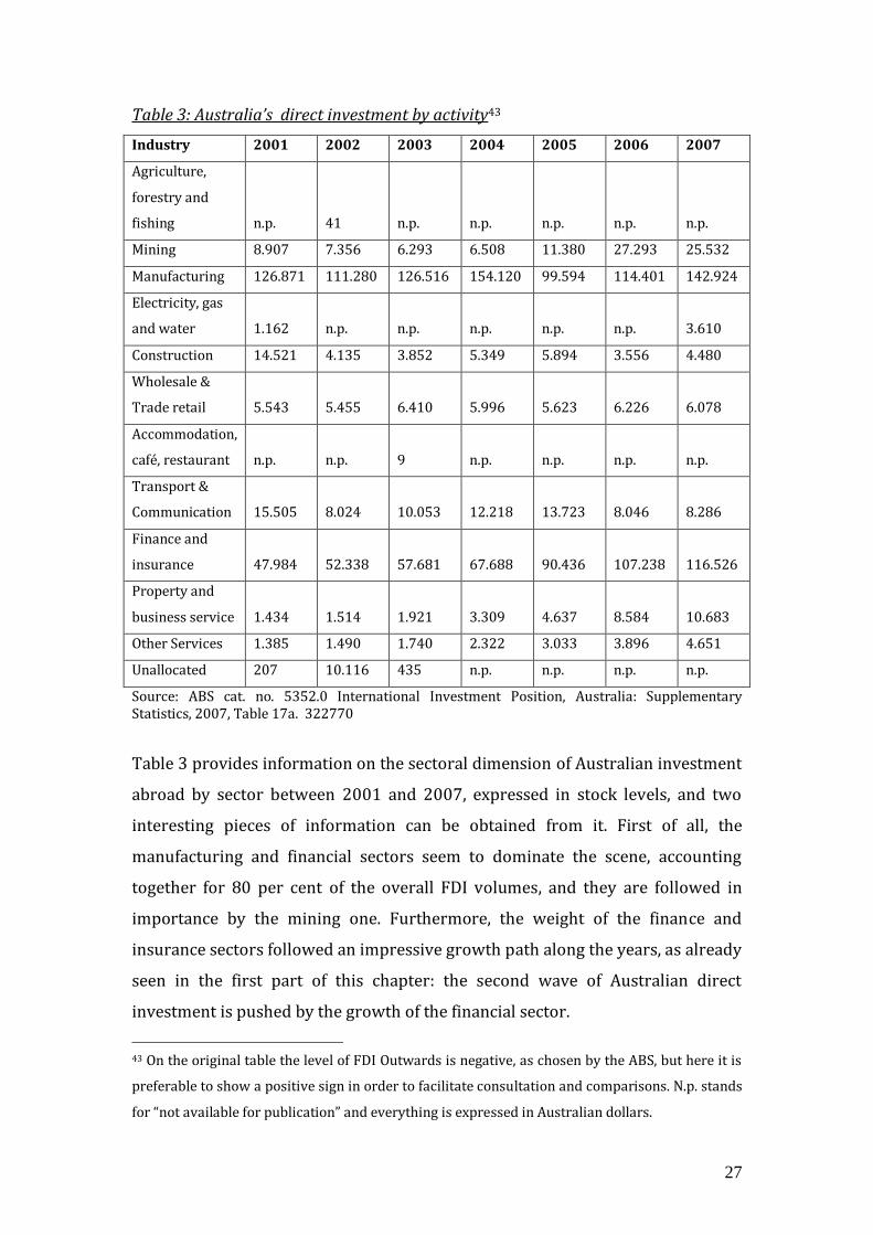
Table 3: Australia’s direct investment by activity43
Industry 2001 2002 2003 2004 2005 2006 2007
Agriculture,
forestry and
fishing n.p. 41 n.p. n.p. n.p. n.p. n.p.
Mining 8.907 7.356 6.293 6.508 11.380 27.293 25.532
Manufacturing 126.871 111.280 126.516 154.120 99.594 114.401 142.924
Electricity, gas
and water 1.162 n.p. n.p. n.p. n.p. n.p. 3.610
Construction 14.521 4.135 3.852 5.349 5.894 3.556 4.480
Wholesale &
Trade retail 5.543 5.455 6.410 5.996 5.623 6.226 6.078
Accommodation,
café, restaurant n.p. n.p. 9 n.p. n.p. n.p. n.p.
Transport &
Communication 15.505 8.024 10.053 12.218 13.723 8.046 8.286
Finance and
insurance 47.984 52.338 57.681 67.688 90.436 107.238 116.526
Property and
business service 1.434 1.514 1.921 3.309 4.637 8.584 10.683
Other Services 1.385 1.490 1.740 2.322 3.033 3.896 4.651
Unallocated 207 10.116 435 n.p. n.p. n.p. n.p.
Source: ABS cat. no. 5352.0 International Investment Position, Australia: Supplementary Statistics, 2007, Table 17a. 322770
Table 3 provides information on the sectoral dimension of Australian investment
abroad by sector between 2001 and 2007, expressed in stock levels, and two
interesting pieces of information can be obtained from it. First of all, the
manufacturing and financial sectors seem to dominate the scene, accounting
together for 80 per cent of the overall FDI volumes, and they are followed in
importance by the mining one. Furthermore, the weight of the finance and
insurance sectors followed an impressive growth path along the years, as already
seen in the first part of this chapter: the second wave of Australian direct
investment is pushed by the growth of the financial sector.
43 On the original table the level of FDI Outwards is negative, as chosen by the ABS, but here it is
preferable to show a positive sign in order to facilitate consultation and comparisons. N.p. stands
for “not available for publication” and everything is expressed in Australian dollars.
28
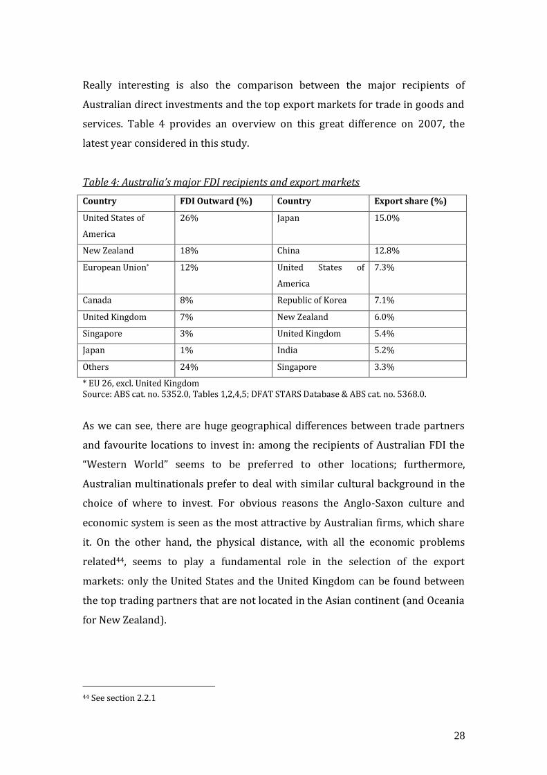
Really interesting is also the comparison between the major recipients of
Australian direct investments and the top export markets for trade in goods and
services. Table 4 provides an overview on this great difference on 2007, the
latest year considered in this study.
Table 4: Australia’s major FDI recipients and export markets
Country FDI Outward (%) Country Export share (%)
United States of
America
26% Japan 15.0%
New Zealand 18% China 12.8%
European Union* 12% United States of
America
7.3%
Canada 8% Republic of Korea 7.1%
United Kingdom 7% New Zealand 6.0%
Singapore 3% United Kingdom 5.4%
Japan 1% India 5.2%
Others 24% Singapore 3.3%
* EU 26, excl. United Kingdom Source: ABS cat. no. 5352.0, Tables 1,2,4,5; DFAT STARS Database & ABS cat. no. 5368.0.
As we can see, there are huge geographical differences between trade partners
and favourite locations to invest in: among the recipients of Australian FDI the
“Western World” seems to be preferred to other locations; furthermore,
Australian multinationals prefer to deal with similar cultural background in the
choice of where to invest. For obvious reasons the Anglo-Saxon culture and
economic system is seen as the most attractive by Australian firms, which share
it. On the other hand, the physical distance, with all the economic problems
related44, seems to play a fundamental role in the selection of the export
markets: only the United States and the United Kingdom can be found between
the top trading partners that are not located in the Asian continent (and Oceania
for New Zealand).
44 See section 2.2.1

29
CHAPTER FOUR
4. METHODOLOGY
This section illustrates the model built for the study; since the approach followed
is of a “general-to-specific” type, it also describes the improvements of the
general model and the tests applied to it. A description of the econometric
procedures in the choice of the most robust variables is also found in the chapter.
4.1 Variables selection process
As already discussed in section 2, previous studies have assessed the role played
by several different variables in the attempt to explain the reasons for FDI. This
study tries to include all the variables frequently used in econometric modelling
and especially the list of crucial factors suggested by Lim (2001) is taken into
consideration. The problem of transforming a theoretical model into a testable
model arises due to the scarcity of economic data, especially in the developing
countries45. To overcome this problem, many authors had to proxy variables
rather than the needed variables; obviously this approach generates simpler
models with a consequent loss of significance. In this section we show the
variables chosen to build our models. The next chapter will provide a full
explanation of the determinants included in our model.
The choice of the variables is never easy but we first focus on building a general
model including most of the determinants highlighted in chapter two: the proxy
chosen for market size is called GDP while production factors are represented by
45 Problems with lacking data can also occur in developed countries; en example lies in the
collection of FDI that it isn’t equal for all the countries and in different years, both in the
definition and collection system. Tcha (1999, p. 90) finds a different definition in Australian
Bureau of Statistics between years before and after 1985.

30
GDPCAP (the variable WAGE is specific only for some country so implies a
further analysis). Openness of trade and distance proxies are named respectively
OPEN and DIST while agglomeration effects with AGGLO. RER, RERVOL and
LANG stand respectively for real exchange rate, real exchange rate volatility and
social determinants. In the end DEMO gives the effects of country risk variable on
Australian direct investment. AIA represents the amount of Australian direct
investments abroad. It is worth mentioning that data are ordered in a panel in
order to capture the two-dimensional nature of the observations46.
4.2 Estimation method
4.2.1 Econometric models
With this choice of explanatory variables the general model takes the form of:
AIAjt = αGDPjt + βGDPCAPjt + γDISTjt + δOPENjt + εRERjt + ζRERVOLjt + ηLANGjt +
θAGGLOjt + λDEMOjt + C
where j stands for the host country and t represent the year the investment takes
place.
Employing this general model a first analysis is made, with the help of the
econometric software Eviews: we decided to run a first and basic pooled analysis
using the technique known as the ordinary least squares (OLS) however
conscious that other approach could be taken47.
46 We must take into account that two variables, LANG and DIST, do not change over years. They
will be fully analysed in the next chapter.
47 From Wezel (2003) we know that such an econometric tool is not the most appropriate
because of the particular nature of the subject analysed and a more technical problem: in fact the
geographical proximity of the host countries (South American countries) suggests the SUR
estimation method to be preferable because it corrects for correlation of the error terms (see p.
26). In principle, we do not have to face such a problem because Australian investments
recipients are located all over the World. Furthermore, the SUR technique requires the number of

31
According to Tcha (1999) then, we apply the OLS and we use these results as the
basis of our analysis; after we discuss the preliminary results, paying attention to
all the possible problems they could carry (serial correlation and
heteroscedasticity for example), we can run a Hausman specification test to see if
we may apply a random effects model or we have to use a fixed effects model.
Again, the improved model is studied and the possible tests and correction
applied. The last analytical technique we use is known as extreme bounds
analysis, widely explained in the next paragraph, and permits our model to get
rid of the less significant variables and construct a new model that takes into
account only the most robust determinants. A final and stronger model is then
obtained.
A further step in our research is made when a new model is built with the
introduction of a more specific variable, WAGE, instead of the generic one
GDPCAP as proxy of production factor costs. The same tests already run on the
original model are performed to see the reactions this change can bring.
However, we need to be aware of the fact that the number of countries included
in the research abruptly decreased from 32 to 15 and the years from 16 to 15.
4.2.2 The extreme bounds analysis
Furthermore, general models are often improved by getting rid of the variables
found less robust and the literature offers different approaches to this “filtering”
operation: for example Deichmann (2004) refines a general model, including ten
explanatory variables, and ends up having a model that takes into consideration
the possible correlation problems between these variables by using a simple
correlation matrix. The same operation can be found in Majocchi and Strange
(2007). A different approach is taken by Levine and Renelt (1992): they test
periods to be greater than the countries we want to analyse and this is definitely not our case
(because we analyse 32 countries and 16 years whereas Wezel studies 8 countries and 10 years).

32
their simple model through a process based on the Extreme Bounds Analysis
(EBA)48 to include in the final model only the most robust variables.
The EBA tests the robustness of each variable using a regression of the form:
γ = αj + βyj * y + βzj * z + βxj * xj + ε
where z is the variable tested, y is a vector of variables taken as fixed (so they are
always included in each regression) and xj a vector of three variables, changing at
every regression and taken from the pool of variables the model wants to test.
For example, being N a pool of 9 independent variables49 (so N equal to 9),
defining them VAR1, VAR2, VAR3 and so on till VAR9, taking a generic variable
DEP as dependent variable, the EBA checks the robustness of every single
variables in the following way:
DEP = α + β1VAR1 + β2VAR2 + β3VAR3 + β4VAR4 + β5VAR5 + β6VAR6
+ β3VAR3 + β4VAR4 + β5VAR5 + β7VAR7
+ β3VAR3 + β4VAR4 + β5VAR5 + β8VAR8
+ β3VAR3 + β5VAR5 + β6VAR6 + β7VAR7
…
+ β3VAR3 + β7VAR7 + β8VAR8 + β9VAR9
In this case, xj is a vector of three variables taken from VAR4 to VAR9 and y is the
couple VAR1 and VAR2. The variable tested, the z of the EBA regression, in this
case is VAR3 and can be defined as robust if it is always found significant when
combined with all the other variables; to check the significance the lower and the
48 The EBA process was introduced by Leamer (1983, 1985).
49 The choice of N equal to 9 in this example makes easier to understand the process because in
this research 9 independent variables are used to explain the determinants of the dependent
variable FDI.
33
upper extreme bounds50 have to be compared: if they are both negative or both
positive the variable is robust. Obviously, the same procedure has to be applied
to all the other variables (VAR4 till VAR9). The test is really strong and it has
been criticized by Sala-i-Martin (1997) for being too selective; for this reason he
suggests a different version of the EBA. Another problem of the EBA lies in the
fact that the choice of the “fixed” variables doesn’t follow a predetermined path;
in the literature, in fact, there are different examples: Wezel (2003) uses GDP and
a variable that captures the risk (political, economical) of investing in a
country51, Mauro (1995) on the other hand opts for GDP, population growth and
secondary education. A possible way to choose the fixed variables is to run the
EBA regressions with the determinants of interest and find a robust variable,
then run again with this variable taken as fixed and so on.
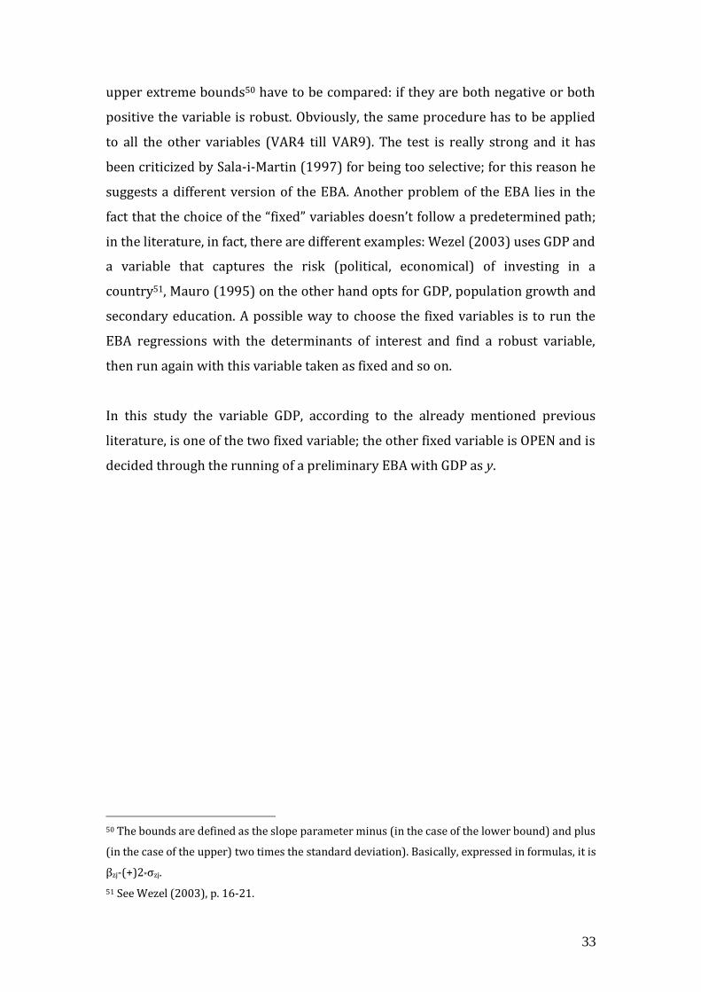
In this study the variable GDP, according to the already mentioned previous
literature, is one of the two fixed variable; the other fixed variable is OPEN and is
decided through the running of a preliminary EBA with GDP as y.
50 The bounds are defined as the slope parameter minus (in the case of the lower bound) and plus
(in the case of the upper) two times the standard deviation). Basically, expressed in formulas, it is
βzj-(+)2*σzj.
51 See Wezel (2003), p. 16-21.

34
CHAPTER FIVE
5. VARIABLES
In chapter 2 we have reviewed the existing literature and the theory behind it
supporting the choice of the explanatory variables we plan to analyse in our
empirical work; now, our study focuses on the illustration of the variables we
decided to use in building the econometric model depicted in chapter four. In
doing this, we first present the dependent variable and then we turn to the
explanatory variables.
5.1 Endogenous variable
In the literature there is no unanimously accepted method of measuring FDI;
different authors chose to work with different measures (Wezel, 2003; Tcha,
1999). Therefore, the choice between using FDI stocks or flows as dependent
variable is not an easy one, as both carry advantages and disadvantages; for
example Wezel (2003) prefers to deal with flows in his study and enounces a list
of distorting factors implied in the choice of stock. These disadvantages,
however, are found to be mostly country specific52. In our analysis stocks are
used rather than flows. In doing so, we follow the large majority of the analyses
on the determinants of inward and outward FDI and as a result, a comparison
with previous studies53 is possible; furthermore, stocks are a better indicator of
the activity in the foreign location because they show the overall amount of
52 For example, German FDI stocks are recorded in the form of balance-sheet book values and this
implies differences, in case of takeovers, between these values and the transaction data which are
recorded at market values in the balance of sheet. Furthermore, individual recipient abroad are
not listed in the Bundesbank’s statistics and this prevents a sectoral analysis from being done.
For an exhaustive explanation, see Wezel (2003), p. 4-5.
53 See among the others Tcha (1999) and Deichmann (2004).

35
capital invested. Another reason for this choice is that flows can massively differ
across years making it very difficult to carry out any specific analysis over time.
We use the stock level of Australian investment abroad collected by the
Australian Bureau of Statistics (ABS 2001, 2007) and our study covers a time
period of 16 years, from 1992 to 2007, and 32 countries54 representing almost
90% of the total Australian outward FDI. The ABS defines the direct investment
following the recommendation of the IMF Balance of Payments Manual so “the
concept of direct investment is based on an investor resident in one economy –
known as the direct investor – obtaining a lasting interest in an enterprise
resident in another economy – the direct investment enterprise”55 (OECD, 2004).
Lasting interest means that the relationship between the investor, which has to
exert a significant influence in the decision making process, and the enterprise
must be of long time. The ownership by the investor, to play a significant
influence, must be of ten per cent or more of the ordinary share or voting stock.
5.2 Exogenous variables
In this section we describe the variables used to build the model of our work and
we go through the determinants of FDI analysed in chapter 2. We also try to
show why some variables have not been included in the econometric models.
5.2.1 Variables included in the analysis
Market size
To capture market size we decide to follow the examples of the studies
mentioned in section 2.2.1 and we collect data on GDP for the 32 countries
54 For the list of the list of the countries analysed in this study, see Appendix A, Table A-1. Among
the important recipients only Taiwan is not considered because of the lack of several data,
especially due to Chinese agreement with the World Bank.
55 See p. 387-388 of OECD (2004). International Direct Investment Statistics Yearbook 1992-2003.
For a more exhaustive explanation of definitions and methods followed by ABS look at ABS
(1998).

36
recipients of Australian direct investment and for the 16 years considered in our
analysis. The data are taken from the World Bank website, in particular from the
World Development Indicators (WDI) database. The advantage of using this
proxy is that all the countries and time periods are fully recorded so there are no
missing data.
Production factor costs
Production costs play a fundamental role in several studies; in our research we
have to face an important data shortage regarding the wages of the recipient
countries. For this reason we choose, following Majocchi and Strange (2007), to
take GDP per capita as proxy of production factor costs56. As for GDP, data are
taken from the World Bank (WDI). However, as explained in section 4.2.1 we also
build a model using the data on wages taken from the Occupational Wages
around the World (OWW) database, derived from ILO October Inquiry
database57; unfortunately there are data only available for 15 years, from 1993
to 2007, and for 15 countries (listed in Appendix A, Table A-1) where Australian
investments are prominent. As a result, this additional analysis can count on
better indicators but has less observations than the previous model.
Economic distance / transport costs
The choice of the most suitable proxy for economic distance has not been
difficult since we decide to follow Deichmann’s (2004) example and consider the
geographical distance between Australia’s most important economic centre
(Sydney), and the leading economic centers of the recipient countries (for
56 We know that the assumption that all the costs of production are given by labour wages and
that all the wealth of a person, represented by GDP per capita, comes only from the wage is
definitely a really strong assumption but we prefer to lose some accuracy for an increase of the
number of observations.
57 The OWW database includes data taken from ILO (http://laborsta.ilo.org Table 01), they are
turned into a normalized wage rate for each occupation and male worker. The database can be
found at http://www.nber.org/oww/.

37
example New York for the United States, London for the United Kingdom, Paris
for France and so on; Appendix A, Table A-2). Distances are expressed in
kilometres and calculated as air distance. Obviously, distance does not change
over time, so the fixed period analysis can not take into account this variable.
Agglomeration effect
The agglomeration variable we use here is defined as suggested by Wezel (2003,
p. 22) so we take the moving-three year average of contemporary and lagged
total FDI inwards stocks relative to respective host country GDP. It is important
to notice that total FDI means that not only Australian direct investments have to
be considered but also the investments coming from other countries. Levels of
FDI inflows and GDP of the host countries are taken from the World Bank (WDI).
Openness of trade (trade barriers)
Our study tries to capture the characteristics of the openness of trade variable
choosing as a proxy the widely accepted ratio of the sum of export and import to
GDP. The choice permits the study to be highly related to previous researches. A
lack of data prevents us from using the Freedom to trade with foreigners index,
from the Fraser Institute or the Trade Freedom Index from the Freedom House
website. Import and export data, like for GDP, are available from the World Bank.
Real exchange rate (and exchange rate volatility)
In this study we decided to test both the effects of the real exchange rate level
and of its volatility on the direct investment. The nominal exchange rate has been
collected from the Reserve Bank of Australia archives and the real exchange rate
has been computed following its recommendations (RBA, 2001). For what may
concern exchange rate volatility, our research follows the study of Hubert and
Pain (1999) and as a result, volatility is defined as a “two-year moving average of
past real exchange rate fluctuations”; technically it is constructed as a variance of
the logarithm of real exchange rate over past years:

38
RERVOL = [(1/2)
2
1i
(( logRER i,t-k – logRER i,t-k+1)/logRER i,t-k+1)2]1/2
Where RERVOL stays for real exchange rate volatility, RER is the real exchange
rate between Australia and the ith country in a year.
Country risk
The choice of the best proxy for the risk that a firm can face when investing in a
certain location was not easy especially because the best indicators, like the
Polity IV dataset, show several missing observations for the countries considered
in our research. Other rich datasets, like for example the Political Risk Service
(PRS), are not freely available, so we have chosen to follow a different approach,
suggested by Narayan (2008), and we used the Polity Score. It can be found on
the Polity IV website and basically it records the political freedom of a country
distinguishing between democracies, fully institutionalized autocracies and
mixed and incoherent regimes (called “anocracies”); these differences are
captured by the Polity Score, ranging from -10 to 10, being 10 the most
institutionalized democracy58. The strength of this dataset is that we can count
on observations for all the years and countries included in our analysis.
Social determinants
As for social determinants, we decided to add a proxy that captures the
relationships existing between Australian culture and the one of the host
country; the choice fell on language similarities, assuming that a more similar
language stimulates the willingness of investing in a specific location. The
approach is supported in the literature by Deichmann (2004). For language
affinity variable we set a scale from 1 to 5 as suggested in McDonald (1997): we
assigned 5 points to English speaking countries, 4 to Germanic (German, Dutch,
58 For more exhaustive information about the Polity Score see:
http://www.systemicpeace.org/polity/polity4.htm

39
etc.) languages, 3 to Romance languages (Italian, French, Spanish, etc.), 2 to
Slavonic (Russian, Polish, etc.) and 1 to languages with negligible connections
with English.
A list of the variables used in this study, with their sources and explanation, can
be found in Appendix A, Table A-4.
5.2.2 Variables excluded from the models
Some of the variables discussed in chapter 2 have been dropped out from the
final econometric model and the reasons are different; for the fiscal incentives
variable we prefer to follow the findings of Reuber and others (1973) and Oman
(2000) consider them too country specific and of secondary importance to be
included in a general analysis. The business climate found in the host countries is
tested using two variables: the country risk proxy captures the political
environment and a social determinant proxy, in the form of language affinity,
gives an idea of cultural similarities. The decision of excluding a Free trade
agreement testable variable has for Australia some specific reason. In fact,
Australia has only 6 free trade agreements59 (ASEAN, Singapore, Thailand,
United States, New Zealand and Chile) but only the one with New Zealand is
totally effective and dated back to 1988. All the others are very recent in time
(around 2005) and at the first stages of their implementation so the possible
effect on FDI could be fully investigated only by the New Zealand-Australia
agreements.
59 For a complete list of Australian free trade agreements (FTA) see Appendix A, Table A-3.

40
CHAPTER SIX
6. EMPIRICAL ANALYSIS
The empirical results based on the panel data described in the previous chapter
aim at examining the drivers of Australian FDI. In order to simplify the
interpretation of our results, Table 5 summarizes the possible effects of the FDI
drivers we have reviewed in chapters 2 and 5.
Table 5 – expected sign of independent variables
Variables Definition Expected valence
GDP Market size +
GDPCAP Production factor costs +
WAGE Production factor costs +
DIST Economic distance + for horizontal FDI
- for vertical FDI
OPEN Openness of trade - for horizontal FDI
+ for vertical FDI
RER Real exchange rate ?
RERVOL RER volatility ?
AGGLO Agglomeration effects +
DEMO Country risk +
LANG Language affinity +
As we can see, and as we have already explained in detail in chapter 2.2.2, the
effect of RER and RERVOL is in general ambiguous. Theory suggests clearer sign
patterns for all the other variables, and this will make the interpretation of our
results easier.
We remember that GDP, GDPCAP, WAGE, DIST, RER and AGGLO are expressed in
logarithmic scale in order to interpret their coefficients as elasticity and more
easily interpret the marginal effects on Australian investment abroad (AIA).
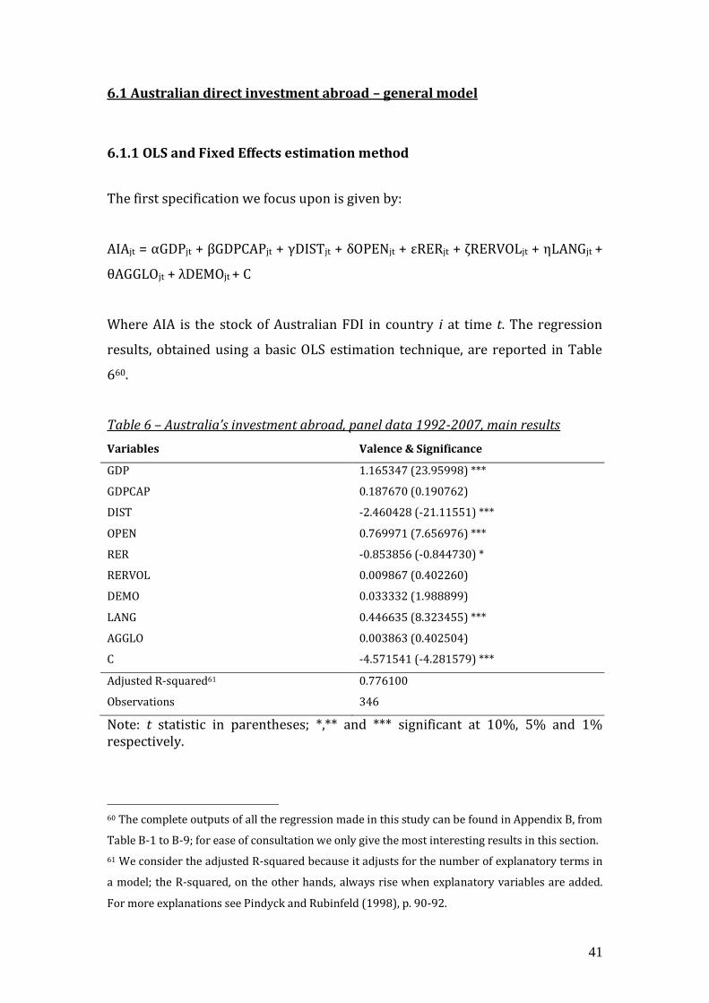
41
6.1 Australian direct investment abroad – general model
6.1.1 OLS and Fixed Effects estimation method
The first specification we focus upon is given by:
AIAjt = αGDPjt + βGDPCAPjt + γDISTjt + δOPENjt + εRERjt + ζRERVOLjt + ηLANGjt +
θAGGLOjt + λDEMOjt + C
Where AIA is the stock of Australian FDI in country i at time t. The regression
results, obtained using a basic OLS estimation technique, are reported in Table
660.
Table 6 – Australia’s investment abroad, panel data 1992-2007, main results
Variables Valence & Significance
GDP 1.165347 (23.95998) ***
GDPCAP 0.187670 (0.190762)
DIST -2.460428 (-21.11551) ***
OPEN 0.769971 (7.656976) ***
RER -0.853856 (-0.844730) *
RERVOL 0.009867 (0.402260)
DEMO 0.033332 (1.988899)
LANG 0.446635 (8.323455) ***
AGGLO 0.003863 (0.402504)
C -4.571541 (-4.281579) ***
Adjusted R-squared61 0.776100
Observations 346
Note: t statistic in parentheses; *,** and *** significant at 10%, 5% and 1% respectively.
60 The complete outputs of all the regression made in this study can be found in Appendix B, from
Table B-1 to B-9; for ease of consultation we only give the most interesting results in this section.
61 We consider the adjusted R-squared because it adjusts for the number of explanatory terms in
a model; the R-squared, on the other hands, always rise when explanatory variables are added.
For more explanations see Pindyck and Rubinfeld (1998), p. 90-92.

42
First, we can notice that four variables out of nine are strongly significant at the
1% level, and that one is weakly significant, at the 10% level; we could also
notice that, looking the F-statistic for the overall significance of the regression,
rejecting the null hypothesis lead to consider our regressors as significant so it
gives credit to the general model applied. Turning to the effect of each individual
variable, we may easily notice how GDP has a strong positive and significant
impact on FDI stocks, as predicted by theory. The positive sign may suggest that
Australian firms tend to locate their production in order to take advantage of
larger markets to exploit scale economies and lower fixed cost per unit of output.
Since we are dealing with elasticity, we can easily interpret the coefficient on
GDP: A one percentage point increase in the latter will lead to a 1.16 per cent
percentage points growth of AIA. A wider discussion deserves the outcomes of
the two variables OPEN and DIST: they are strongly significant (1% level) but
they show different relationship with AIA, respectively positive and negative.
This finding is in accordance with theoretical studies and is consistent with a
vertical motivation behind Australian investments: distance negatively affects
vertical FDI due to higher transport cost while higher openness of trade has a
positive effect on them because of lower barriers (costs) for trades62. Again, we
are considering elasticities but the effect of OPEN is weaker than GDP (around
0.77) while DIST strongly affects vertical investments reducing them by 2.46 per
cent every km farer from Sydney. Also the LANG proxy enters significantly in the
decision to invest abroad, but this result is not surprising if we remember that
four out of the first five destinations of Australian investments are English
speaking countries63. Again this result supports the theoretical predictions. A
different discussion characterizes RER: the significance is weak (at 10% level)
and the negative sign suggests that an appreciation of one unit of the Australian
62 In our work we consider openness of trade as the simple trade shares of a country so we are
conscious our proxy does not perfectly represents the effect of lower trade barriers. Average
tariff rates, export taxes and indices of non-trade barriers would be better proxies but we defend
our choice because it is the most spread through previous research and because we found lack of
data for the above mentioned indicators. For an extensive review of openness proxies see
Yannikaya (2003).
63 See Table 4 in chapter 3.2.
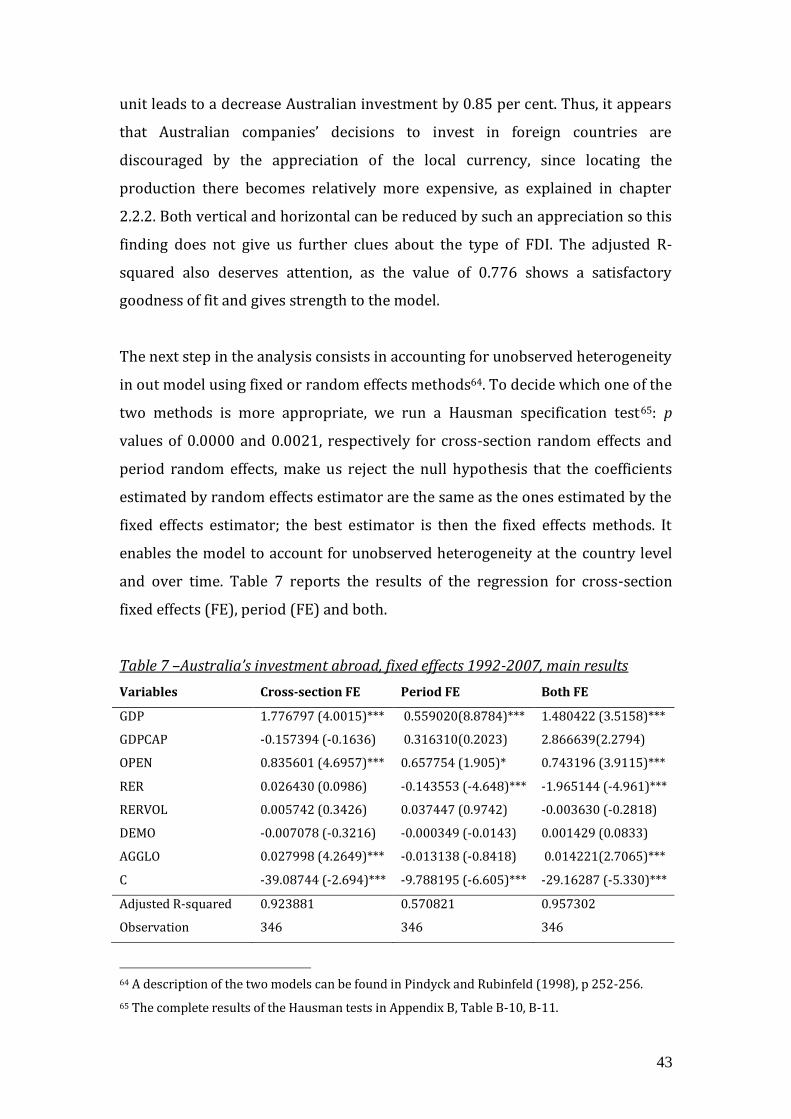
43
unit leads to a decrease Australian investment by 0.85 per cent. Thus, it appears
that Australian companies’ decisions to invest in foreign countries are
discouraged by the appreciation of the local currency, since locating the
production there becomes relatively more expensive, as explained in chapter
2.2.2. Both vertical and horizontal can be reduced by such an appreciation so this
finding does not give us further clues about the type of FDI. The adjusted R-
squared also deserves attention, as the value of 0.776 shows a satisfactory
goodness of fit and gives strength to the model.
The next step in the analysis consists in accounting for unobserved heterogeneity
in out model using fixed or random effects methods64. To decide which one of the
two methods is more appropriate, we run a Hausman specification test65: p
values of 0.0000 and 0.0021, respectively for cross-section random effects and
period random effects, make us reject the null hypothesis that the coefficients
estimated by random effects estimator are the same as the ones estimated by the
fixed effects estimator; the best estimator is then the fixed effects methods. It
enables the model to account for unobserved heterogeneity at the country level
and over time. Table 7 reports the results of the regression for cross-section
fixed effects (FE), period (FE) and both.
Table 7 –Australia’s investment abroad, fixed effects 1992-2007, main results
Variables Cross-section FE Period FE Both FE
GDP 1.776797 (4.0015)*** 0.559020(8.8784)*** 1.480422 (3.5158)***
GDPCAP -0.157394 (-0.1636) 0.316310(0.2023) 2.866639(2.2794)
OPEN 0.835601 (4.6957)*** 0.657754 (1.905)* 0.743196 (3.9115)***
RER 0.026430 (0.0986) -0.143553 (-4.648)*** -1.965144 (-4.961)***
RERVOL 0.005742 (0.3426) 0.037447 (0.9742) -0.003630 (-0.2818)
DEMO -0.007078 (-0.3216) -0.000349 (-0.0143) 0.001429 (0.0833)
AGGLO 0.027998 (4.2649)*** -0.013138 (-0.8418) 0.014221(2.7065)***
C -39.08744 (-2.694)*** -9.788195 (-6.605)*** -29.16287 (-5.330)***
Adjusted R-squared 0.923881 0.570821 0.957302
Observation 346 346 346
64 A description of the two models can be found in Pindyck and Rubinfeld (1998), p 252-256.
65 The complete results of the Hausman tests in Appendix B, Table B-10, B-11.

44
Commenting the results, it is worth mentioning that, since LANG and DIST
variables do not change over years, they can not be included in the model and
this implies the loss of two highly significant determinants. A quick comparison
between the three outputs confirms the strong significance of GDP and OPEN
(even if in the period FE case the significance is weaker) also when cross-country
and period FE are considered. Looking at the magnitude of the coefficient of
OPEN we can see that it doesn’t change too much from the OLS model and the
sign is still positive; greater changes (compared to OLS results) occur for GDP
when cross-section FE and period FE are taken into account: stronger positive
effect for the first (1.77) and smaller positive effect for the second (0.56). This
could suggest that the differences between countries tend to empower the
relationship between GDP and AIA, while the effect is mitigated across years. The
other variable found significant in the first regression was the RER and Table 7
provides an interesting picture: when cross-section FE are applied the variable
loses significance while the opposite happens when corrected with period FE
(significant at 1%) level. This fact may suggest that year fixed effects model can
better represent the influence (still negative even if weaker) on Australian
investment. The last driver found significant, when corrected for FE, is AGGLO
and this is an important difference with the OLS output. The sign of the
coefficient confirms the theoretical predictions developed in chapter 2, but it can
be detected only with cross-country FE; this could mean that agglomeration
effects play a role only if heterogeneity across country is considered. Its impact
during years seems to be not significant. However, the fact that its effect on AIA
is very weak (0.028 for cross-section FE and 0.014 for both the FE) could suggest
that Australian investments are only marginally affected by the size of the
existing FDI stock. For these reasons the results are similar to the OLS
regressions and the corrections applied do not change the situation depicted in
the general model analysis.
A final look at the adjusted R-squared shows that the model fits the data very
well when cross-section FE are considered (0.923) and a little weaker, but still
satisfactory, with period FE (0.57). The lower value of period FE adjusted R-
squared may suggest that the inclusion of year-specific effects in our research
weakens the fit of the regression.

45
6.1.2 Extreme bounds analysis
So far the analysis of the determinants of Australian investments abroad has
shown the importance of two variables: GDP and OPEN and the importance of
RER, all tested with fixed effects. Also DIST and LANG are found to be strongly
significant, buy unfortunately they can not be added to the fixed effects models.
Following a “general-to-specific” approach, we try now to narrow down the
number of variables included in the general model to create a new and more
robust one through the econometric technique known as the extreme bounds
analysis (EBA). The results from this method are reported in Table 8.
Table 8 – Extreme bounds analysis
Variables Lower bound Upper bound
GDPCAP -0.41511 0.226421
DIST -1.92122 0.395166
LANG* 3325.497 8441.698
RER -3.14209 6.183354
RERVOL -1955.69 1206.146
DEMO -591.796 885.4638
AGGLO -1045.19 2030.478
Fixed variables: GDP and OPEN66. Regressions include the fixed variables plus one of those listed above (variables of interest and three of the pool of remaining variables at a time. * denotes robust variables as found by EBA.
Only LANG is found robust at the EBA test so we can build a new model including
only the three robust variables: GDP chosen following literature examples, OPEN
through preliminary EBA and LANG as explained above.
AIAjt = αGDPjt + δOPENjt + ηLANGjt + C
66 The choice of the fixed variables is explained in chapter 4.2.2.

46
Table 9 – Australia’s investment abroad, 1992-2007, main results
Variables Valence & Significance
GDP 0.661591 (16.09002)***
OPEN 0.642358 (8.076970) ***
LANG 0.402703 (9.536579) ***
C -11.80753 (-10.35981) ***
Adjusted R-squared 0.535784
Observations 441
Note: t statistic in parenthesis; *,** and *** significant at 10%, 5% and 1%
respectively
Table 9 shows the results of the regression OLS applied to the robust model;
again, the three variables are found highly significant at 1% level so further
attention must be paid to the magnitude of the coefficient if compared to results
of Table 6. The coefficients of OPEN and LANG are very similar but differences
are seen in GDP: in fact, the coefficient of the robust model shows the same signs,
but smaller magnitudes and this fact could imply that the general model
overestimates it. The robust model is supported also by a good value of adjusted
R-squared (0.535). We decided not to apply the FE effects because we could not
include LANG in the models and it would reduce the model only at the study of
two variables67.
6.2 Australian direct investment abroad – robustness check for wage
variable
As explained in chapter 4.2.1 and 5.2.1 the GDPCAP variable is a weak proxy for
production factors costs and the analyses of section 6.1 show that it is also not
significant. The non significance might be explained by possible measurement
errors. As a result, we build a new model replacing GDCAP with a more precise
WAGE. We also must take into account that, to insert this variable in the model,
67 The behaviour of OPEN and GDP with fixed effects included has been analysed in section 6.1.1
and this is the reason we prefer to study the model with all the robust variables.

47
we have to reduce the sample and subsequently the number of observations68.
Table 10 includes the results of the OLS and the FE regressions.
Table 10 – Australia’s investment abroad, 1993-2007
Variables OLS Cross-section FE
Period FE Both FE
GDP 1.29054(19.238) ***
1.962846 (8.1526) ***
0.519296 (7.1420) ***
1.479300 (2.6311) ***
WAGE -0.007428 (-0.096)
0.082270 (0.2245)
0.260085 (0.6776)
0.347484 (1.0411)
DIST -2.300908 (-15.618) ***
OPEN 0.688378 (4.6671) ***
0.436270 (1.8432) *
0.979021 (5.3320) ***
0.555378 (3.4696) **
RER -0.305356 (-2.7820) ***
0.659184 (1.2172)
-0.641162 (-6.8257) ***
-0.355091 (-0.6448) ***
RERVOL -0.035264 (-1.2045)
0.007263 (0.3617)
-0.070290 (-5.6564)
0.010122 (0.7419)
DEMO 0.092836 (1.8469) *
0.164949 (0.981674)
0.286739 (5.8415) ***
0.065443 (0.5906)
LANG 0.078143 (1.7004) ***
AGGLO 0.024254 (2.4723) **
0.030923 (4.4192) ***
0.046689 (3.078290) ***
0.014663 (2.9945) ***
C -6.306084 (-3.960357) ***
-48.07001 (-9.0930) ***
-4.768916 (-1.1967) ***
-49.16392 (-3.4313) ***
Adjusted R-squared
0.824758 0.927551 0.694169 0.969796
Observations 197 197 197 197
Note: t statistic in parenthesis; *,** and *** significant at 10%, 5% and 1% respectively.
The object of our robustness check is the effect of labour costs, proxied by WAGE,
on Australian investments and the findings seem to confirm the non significance
of such a variable: in fact, like GDPCAP in the previous analysis, WAGE is never
found significant. This means that even a more precise measure for labour costs
does not make them significant.
Looking at the column of OLS regression we can immediately notice how the
variables GDP, OPEN, DIST, RER and LANG still remain significant, even with
different level compared to the general model analysis. In fact, RER is now
68 The modified model reduces the number of country included in the dataset from 32 to 15 and
excludes the observations for the year 1992. Luckily, the major destinations of Australian FDI are
still included in the analysis.
48
strongly significant. The coefficients of GDP, OPEN and DIST are very similar to
the ones estimated in the model including GDPCAP so the analysis is the same we
did in the previous section. The interesting part of this analysis lies in the
magnitude of RER and LANG, far smaller than the original model, and moreover
in the variable DEMO and AGGLO. DEMO is found significant also when period FE
are applied (but not with cross-section FE) showing a positive coefficient: this is
not surprising because more points a country has on the democracy scale used in
our study, the more attractive for investment it is. Here, an increase of one point
in the scale brings an increase of 0.09 and 0.28 per cent (with period FE) of AIA.
For AGGLO, there is an important proof of significance because now we do not
have to apply the correction for fixed effects (which however confirms) to see its
impact on AIA69. The high adjusted R-squared (0.824) gives strength to the
model and to our findings.
In sum, this further analysis failed in the attempt to introduce a more explicative
variable for labour costs but the fact that, also in presence of a small sample, the
outputs are basically the same of the original model could suggest Australian
investments not to be attracted by lower labour costs, regardless of the proxy
chosen to study them.
69 However, it is important to note that the effect of AGGLO on AIA is significant but still very
close to zero.

49
CHAPTER SEVEN
7. CONCLUSIONS
This work investigated the reasons which drive Australian investments abroad
and the empirical results suggest that both vertical and horizontal motives play
an important role.
Among the determinants found significant, vertical characteristics are shown by
the sign of the coefficient of the variable which captures openness of trade (trade
barriers): the positive sign, according to theory, suggests that vertical
investments are more likely, since vertical investments imply trade between the
FDI source and destination countries. This interpretation is consistent with other
findings of our analysis. In particular, Australian firms are more likely to locate
their investments in countries which are geographically closer to them.
Therefore, openness of trade and distance findings give a vertical shape to
Australian investments.
We found also that Australians companies share some preference for horizontal
FDI as well, as indicated by the importance of market size for their investments.
In fact, as predicted by theory, horizontal investments are strongly attracted by
large markets because in larger economies is possible to reduce the cost implied
in supplying them and it is easier to adapt to changes in local customs. The
importance of horizontal FDI is witnessed also by the preference for countries
who share the same language as favourite locations. A closer culture, in fact,
increases the possibility to successfully enter the market.
Nothing can be said about the type of investment chosen by Australian firms
when we consider the other significant drivers. Real exchange rate movements
do affect in the same way both vertical and horizontal investments, and in our
work we found a negative influence on them deriving from a possible

50
appreciation of the local currency. Hence, Australian firms found to be sensitive
to fluctuations. It is also interesting to note that the presence of other FDI in a
region (agglomeration effect) can attract Australian multinationals, even if the
relationship seems to be really weak. Again, no further information about the
nature of the investment can be taken from this variable.
Political risk and especially production factor costs do not play a significant role
but the reasons behind this fact could be different. For political risk the choice of
the proxy, in our work represented by the presence of democracy in the host
country, could be too generic. We must notice, however, that the sample we used
does not include countries which reported important political risks during the
period analysed and this could explain the absence of significance. For
production factor costs, on the other hand, the problem does not lie in the choice
of the proxy, as showed by the robustness check we applied. For this reason the
non significance can not be explained by a lack of accuracy but more probably,
Australian firms tend to consider other factors as main drivers of their
investments abroad.
In sum, Australian investments abroad are characterized by some typical vertical
feature, like the preference for trade open countries, favourably close to their
home market, and some horizontal trait, like the orientation towards large host
economies which also share similar cultural roots. The possibilities of cheaper
investments, offered by the host country exchange rate movements, also play an
important role, and agglomeration effect makes clustering attractive, even if in a
very weak way. Labour costs do not significantly affect the choice of investing
abroad, like political risks.

51
REFERENCES
Agarwal, J. (1980). Determinants of foreign direct investments: A survey.
Weltwirschaftliches Archiv 116(4), 739-773.
Agiomirgianakis, G., Asteriou, D. & Papathoma, K. (2003). The determinants of
foreign direct investment: a panel data study for the OECD countries.
Discussion Papers 03/06. City University London.
Aizenman, J. (1992). Exchange rate flexibility, volatility, and the patterns of
domestic and foreign direct investment, NBER Working Paper 3953.
Anderson, E. & Gatignon, H. (1986). Modes of foreign entry: a transaction cost
analysis and propositions. Journal of International Business Studies 17, 1-26.
Armstrong, S. (2009). Japanese FDI in China: determinants and performances.
Asia Pacific Economic Papers 378, 1-34.
Aulakh, P.S. & Kotabe, M. (1997). Antecedents and performance integration of
channel integration in foreign markets. Journal of International Business
Studies 28 (1), 145-175.
Australia ---- Bureau of Statistics (1998). Cat. no. 5331.0 Balance of Payments and
International Investment Position, Australia: Concepts Sources and Methods,
1998.
Australia ---- Bureau of Statistics (2002). Cat. no. 5352.0 International Investment
Position, Australia: Supplementary Statistics, 2000-2001, Table 6.
Australia ---- Bureau of Statistics (2007). Cat. no. 5352.0 International Investment
Position, Australia: Supplementary Statistics, 2007, Tables 1, 2, 4, 5, 17a.

52
Australia ---- Bureau of Statistics (2007). Cat. no. 5368.0 International Trade in
Goods and Services, December 2007.
Australia ---- Reserve Bank of Australia (2001). Measuring the Real Exchange
Rate, November 2001. Available at:
http://www.rba.gov.au/PublicationsAndResearch/Bulletin/bu_nov01/bu_1101_
2.pdf
Bandelj, N. (2002). Embedded economies: social relations as determinants of
foreign direct investment in Central and Eastern Europe. Social Forces 81 (2),
411-444.
Bevan, A.A. & Estrin, S. (2004). The determinants of foreign direct investment
into European transition economies. Journal of Comparative Economics 32
(4), 775-787.
Beyer, J. (2002). Wie erfolgreich sind Maßnhamen zur Förderung von
ausländischen Direktinvestitionen? Empirische Befunde aus den
Transformationsländern. Zeitschrift für Wirtschaftpolitik 51 (1), 63-83.
Brainard, S.L. (1997). An empirical assessment of the proximity-concentration
trade-off between multinational sales and trade. American Economic Review
87 (4), 520-544.
Brzozowski, M. (2003). Exchange rate variability and foreign direct investment –
Consequences of EMU enlargement. CASE Studies and Analyses 258, 1-26.
Buckley, P.J., Devinney, T.M. & Louviere, J.J. (2007). Do managers behave the way
theory suggests? A choice-theoretic examination of foreign direct investment
location decision-making. Journal of International Business Studies 38, 1069-
1094.
53
CIA, The World Factbook (2009). Website link:
https://www.cia.gov/library/publications/the-world-
factbook/rankorder/2004rank.html?countryName=Australia&countryCode=
AS®ionCode=au#AS
https://www.cia.gov/library/publications/the-world-
factbook/rankorder/2199rank.html?countryName=Australia&countryCode=
AS®ionCode=au#AS
Darby, J., Hughes Hallet, A., Ireland, J. and Piscitelli, L. (1999). The impact of
exchange rate uncertainty on the level of investment. Economic Journal 109,
55-67.
Dees, S. (1998). Foreign direct investment in China: determinants and effects.
Economics of Planning 31, 175-194.
Deichmann, J. (2004). Origins of foreign direct investment in Poland. Journal of
International Business Studies, 1989-2001 vol. 10(1), 12-28.
Deng, P. (2003). Foreign investments from emerging countries: the case of China.
Journal of Leadership and Organizational Studies. Website link:
http://www.entrepreneur.com/tradejournals/article/111769221_1.html
Duncan, M.H. (2000). Country risk and foreign direct investment. Business
Economics 35 (1), 33-40.
Dunning, J.H. (1977). Trade, location of the economic activity and the MNE: a
search for an eclectic approach. In The International Allocation of Economic
Activity, O. Bertil et al., eds. Proceeding of Noble Symposium held in Stockholm,
London: McMillan.
---- (1980). Toward an eclectic theory of international production: some
empirical tests. Journal of International Business Studies 11, 9-31.

54
---- (2000). The eclectic paradigm as an envelope for economic and business
theories of MNE activity. International Business Review 9, 163-190.
Edwards, R.W. & Buckley, P.J. (1996). Exporting costs: a key factor in FDI
decisions for Australian Multinationals. Monash University Working Paper
Series 96 (2), 1-29.
Eiteman, D., Moffett, M. & Stonehill, A. (1995). Multinational Business Finance.
Addison-Wesley Publishing Company.
Ekholm, K. (1998). Proximity advantages, scale economies and the location of
production. The Geography of Multinational Firms, p. 5976.
Everhart, S.S. & Sumlinski, M.A. (2001). Trends in private investment in
developing countries – statistics for 1970-2000 – and the impact on private
investment of corruption and the quality of public investment. IFC Discussion
Paper 44.
Feenstra, R.C. & Hanson G.H. (1997). Foreign direct investments and relative
wages: evidence from Mexico’s Maquiladoras. Journal of International
Economics 42, 371-393.
Formica, S. (1996). Political risk analysis in relation to foreign direct investment:
a view from the hospitality industry. Tourism Review 51 (4), 15-23.
Froot, K.A. & Stein, J.C. (1991). Exchange rate and foreign direct investment: an
imperfect capital markets approach. The Quarterly Journal of Economics 106,
1191-1217.
Goldberg, C. and Kolstad, C. (1995). Foreign direct investment, exchange rate
volatility and demand uncertainty. International Economic Review 36, 855-
873.

55
Guisinger, S. (2001). From OLI to OLMA: incorporating higher levels of
environmental and structural complexity into the eclectic paradigm.
International Journal of Economics and Business 8 (2), 257-272.
Hakkala, K., Norbäck, P. & Svaleryd, H. (2008). Asymmetric effects of corruption
of FDI: evidence from Swedish multinational firms. The Review of Economic
and Statistics, MIT Press 90(4), 627-642.
Hausmann, R. & Fernàndez-Arias, E. (2001). Foreign direct investment: good
cholesterol? In OECD (Ed): Foreign direct investment versus other flows to
Latin America, Paris.
Henisz, W. (2000). The institutional environment for multinational investment.
Journal of Law and Economics and Organization (16), 334-364.
Hines, J. (1995). Forbidden payments: foreign bribery and American business
after 1977. NBER Working Papers 5266.
Hubert, F. & Pain, N. (1999). Innovation and the regional and industrial pattern
of German foreign direct investment, in Barrell, R. & Pain, N. (Eds.)
Investment, innovation and the diffusion of technology in Europe. Cambridge
University Press (Mass.):168-194.
Johanson, J. & Paul, S. Wiedersheim (1975). The internalization of the firm: four
Swedish cases. Journal of Management Studies 12 (3), 305-322.
Kandiero, T. & Chitiga, M. (2003). Trade openness and foreign direct investment in
Africa, paper prepared for the Economic Society of Southern Africa 2003
Annual Conference, Cape Town. Published in SAJEMS NS 9 (2006), 3: 335-370.
Kang, M. & Park, S. (2004). Korea – U.S. FTA: trade and investment creation
effects and trade structure. KIEP Policy Analysis 4 (12).

56
Khadaroo, A.J. & Seetanah, B. (2007). Transport infrastructure and FDI: lessons
from Sub Saharan African Economies. Presented at the African Economic
Conference (AEC), 15-17 Nov. 2007. UN Conference, Addis Ababa, Ethiopia.
Link:
http://www.uneca.org/aec/documents/Jameel%20Khadaroo_Boopen%20Se
etanah.pdf
Kiyota, K. & Urata, S. (2004). Exchange rate, exchange rate volatility and foreign
direct investment. The World Economy, Blackwell Publishing, 27 (10), 1501-
1536.
Kosteletou, N. & Liargovas, P. (2000). Foreign direct investment and real
exchange rate linkages. Open Economic Review 11, 135-148.
Kravis, I.B. & Lipsey, R.E. (1982). The location of overseas production and
production for export by U.S. multinational firms. Journal of International
Economics 12, 201-223.
Kumar, V. & Subramaniam, V. (1997). A contingency framework for the mode of
entry decision. Journal of World Business 32 (1), 53-72.
Labrianidis, L. (2001). Geographical proximity matters in the orientation of FDI:
the case of Greek FDI in the Balkans. In Petrakos, G. & Totev, S. (2000). The
development of the Balkan region. Aldershot: Ashgate, 463-489.
Leamer, E. (1983). Let’s take the con out of econometric. American Economic
Review 73, 31-43.
---- (1985). Sensitivity analysis would help. American Economic Review 75, 308-
313.
---- (1988). Measures of openness. In Baldwin, R. (Ed): Trade policy issues and
empirical analysis. University of Chicago Press, Chicago (Illinois): 147-200.

57
Levine, R. & Renelt, D. (1992). A sensitivity analysis of cross-country growth
regressions. American Economic Review 82, 942-963.
Lim, E. G. (2001). Determinants of, and the relation between, foreign direct and
growth: a summary of the recent literature. IMF Working Paper, 01/175.
Lipsey, R.E. (2002). Home and host country effects of FDI. NBER Working Paper
9293.
Loungani, P., Mody, A. and Razin, A. (2002). The global disconnect: the role of
transactional distance and scale economies in gravity equations. Scottish
Journal of Political Economies 49(5), 526-543.
Madhok, A. (1998). The nature of multinational firm boundaries: transaction
costs, firm capabilities and foreign market entry mode. International Business
Review 7, 259-290.
Majocchi, A. & Strange, R. (2007). The FDI location decision: does liberalization
matter? Transnational Corporations, 16-2.
Mauro, P. (1995). Corruption and Growth. The Quarterly Journal of Economics
110, 681-712.
McDonald. (1997). The European scene: a geographic perspective. Englewood
Cliffs, New Jersey: Prentice Hall.
Mody, A., Dasgupta, S. & Sinha, S. (1999). Japanese multinationals in Asia: drivers
and attractors. Oxford Development Studies 27, 149-164.
Mody, A. & Srinivasan, K. (1998). Japanese and US firms as foreign investors: do
they march in the same tune? Canadian Journal of Economics 31, 778-799.
58
Mundell, R. A. (1957). International trade and factor mobility. American
Economic Review 47, 321-325.
Nakos, G. & Brouthers, K. D. (2002). Entry mode choice of SMEs in Central and
Eastern Europe. Entrepreneurship Theory and Practice 27 (1), 47-64.
Narayan, P.K. (2008). An econometric model of the determinants of private
investment and a CGE model of the impact of democracy on investment and
economic growth in Fiji. International Journal of Social Economics 35 (12),
1017-1031.
OECD (2004). International Direct Investment Statistics Yearbook 1992-2003,
387-390.
Oman, C. (2000). Policy Competition for Foreign Direct Investment: A Study of
Competition among Governments to Attract FDI. OECD Development Centre,
Paris.
Padilla, L. & Richards, T.J. (1999). Locational determinants of US foreign direct
investment of food and kindred products in Latin America. 1999 Annual
Meeting, August 8-11, Nashville, TN. Link: http://purl.umn.edu/21514
Pan, Y.G. & Tse, D.K. (2000). The hierarchical model of market entry modes.
Journal of International Business Studies 31 (4), 535-554.
Pindyck, R.S. & Rubinfeld, D.L. (1998). Econometric Models and Econometric
Forecasts. (4th edition). McGraw-Hill International Editions.
Pritchett, L. (1996). Measuring outward orientation in LDCs: can it be done?
Journal of Development Economics 49, 307-335.

59
Rafferty, M. & Bryan, D. (1998). Advance Australia everywhere: the case of
Australian foreign direct investment in the United Kingdom in the 1980s and
1990s. Working Papers in Australian Studies, no. 113.
Rafferty, M. & Ham, R. (2004). The global race for FDI: the case of Australian
investment in Europe. In European Union and the race for foreign direct
investment in Europe, ed. Ghauri, P. & Oxelheim, L., Elsevier and Oxford
University Press, London, United Kingdom, 209-236.
Reuber, G.L., Crookel, H., Emerson, M. & Gallais-Hamonno, G. (1973). Private
foreign investment in development. Oxford: Clarendon Press.
Root, F.R. (1994). Entry strategies for international markets. London: Lexington
Books.
Root, F.R. & Ahmed, A.A. (1979). Empirical determinants of manufacturing direct
foreign investment in developing countries. Economic Development and
Structural Change 27, 751-767.
Sala-i-Martin, X. (1997). I just ran four millions regressions. NBER Working Paper
6252.
Schneider, S. & Frey, B.S. (1985). Economic and political determinants of foreign
direct investment. World Development 13, 161-175.
Shatz, H. & Venables, A.J. (2000). The geography of international investment.
World Bank Policy Research Paper 2338.
Singh, H. & Jun, K.W. (1995). Some new evidence on determinants of foreign
direct investment in developing countries. World Bank Policy Research
Working Paper 1531.

60
Smarzynska, B. & Wei, S. (2000). Corruption and composition of foreign direct
investment: firm-level evidence. NBER Working Papers 7969.
Stevens, G. (2000). Politics, economics and investment: explaining plant and
equipment spending by US direct investors in Argentina, Brazil and Mexico.
Journal of International Money and Finance 19, 153-183.
Tarzi, S. (2005). Foreign direct investment into developing countries: impact of
location and government policy. The Journal of Social, Political and Economic
Studies 30 (4), 497-516.
Tcha, M. (1999). A note on Australia’s inward and outward direct foreign
investment. Papers in Regional Science 78, 89-100.
Turner, A.G. & Golub, S.S. (1997). Towards a system of multilateral unit labor
cost-based competitiveness indicators for advanced, developing and
transition countries. IMF Working Papers 97/151.
UNCTAD (2008). World Investment Report 2008. Transnational Corporation and
the Infrastructure Challenge. Country Fact Sheet: Australia
Velde, D.W., te & Bezemer, D. (2006). Regional integration and foreign direct
investment in developing countries. Transnational Corporations 15 (2), 41-
70.
Wezel, T. (2003). Determinants of German foreign direct investment in Latin
America and Asian emerging markets in the 1990s. Discussion Paper 11-03.
Economic Centre Research of the Deutsche Bundesbank.
Wheeler, M. & Mody, A. (1992). International investment location decisions – the
case of US firms. Journal of International Economics 33, 57-76.

61
Woodward, D.P. & Rolfe, R.J. (1993). The location of the export-oriented foreign
direct investment in the Caribbean Basin. Journal of International Business
studies 24, 121-144.
Yannikaya, H. (2003). Trade openness and economic growth: a cross-country
empirical investigation. Journal of Development Economics 72, 57-89.
Zhao, X. & Decker, R. (2004). Choice of foreign market entry mode. Cognitions
from empirical and theoretical studies. Available at:
http://bison.ub.uni-bielefeld.de/volltexte/2004/507/pdf/m_entry.pdf

62
ACKNOWLEDGEMENTS
Special thanks to my Mom and Dad who always supported me both in good and
hard times. I also would like to thank my brother, my grandma and some very
good friend: Fausto, Piazza, Citterio, BigK, Danny Boy, Maurizio (centurione),
Dani, Barza, Manto, Castello, Bas & Taco.
Really sincere thanks also to people who I spent great time with during this
fantastic year: Nora, Mara, Nikki, Nass, Peter, Rie, Sylwia, Inge, the Aussies from
Amsterdam (Lani, Claire, Kat, Sam, Emily), Declan, Rosa, the Englishmen, Bang,
the Irish lads, TOGB and Nico Mekel, the crazy Dutchmen (Paul, Frank, Elroy,
Jeroen, Daniel and Jordy), Esther, Daniela and Kiki, Thomas, M.J. Dundee and the
Joker.
In the end I would like to give thanks to my supervisor Giovanni Facchini who
helped me with this research.

63
APPENDIX A
Table A-1 – list of countries
Argentina Fiji Japan* Russian Federation
Bahrain France Republic of Korea*
Singapore*
Brazil Germany* Malaysia South Africa* Belgium & Luxembourg*
Greece* Mexico Sweden*
Canada* Hong Kong* Netherlands* Switzerland Centr. America & Caribbean
Indonesia New Zealand* Thailand
Chile Ireland* Papua New Guinea
United Kingdom*
China Italy Philippines United States*
The countries marked with * are included also in the second model that tests the
significance of the wages instead of GDP per capita as production costs variable.
Caribbean and Centr. America represents Virgin British Islands, Cayman Islands
and Bermuda.
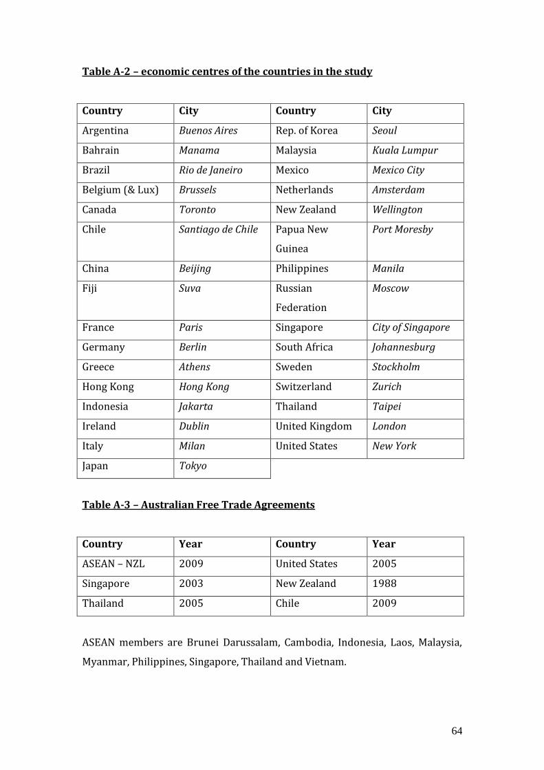
64
Table A-2 – economic centres of the countries in the study
Country City Country City
Argentina Buenos Aires Rep. of Korea Seoul
Bahrain Manama Malaysia Kuala Lumpur
Brazil Rio de Janeiro Mexico Mexico City
Belgium (& Lux) Brussels Netherlands Amsterdam
Canada Toronto New Zealand Wellington
Chile Santiago de Chile Papua New
Guinea
Port Moresby
China Beijing Philippines Manila
Fiji Suva Russian
Federation
Moscow
France Paris Singapore City of Singapore
Germany Berlin South Africa Johannesburg
Greece Athens Sweden Stockholm
Hong Kong Hong Kong Switzerland Zurich
Indonesia Jakarta Thailand Taipei
Ireland Dublin United Kingdom London
Italy Milan United States New York
Japan Tokyo
Table A-3 – Australian Free Trade Agreements
Country Year Country Year
ASEAN – NZL 2009 United States 2005
Singapore 2003 New Zealand 1988
Thailand 2005 Chile 2009
ASEAN members are Brunei Darussalam, Cambodia, Indonesia, Laos, Malaysia,
Myanmar, Philippines, Singapore, Thailand and Vietnam.

65
Table A-4 – List of exogenous variables employed
Variables Definition Dimension/Timing Further explanations
Source
AIA Level of Australian investments abroad
AUS$ million, 1992-2007 Australian Bureau of Statistics
GDP Real absolute GDP
Current US$ World Bank WDI
GDPCAP Real GDP per capita
Current US$ Proxy for wages
World Bank WDI
WAGE Occupational wages
Uniform calibration US$, 1993-2007
normalized wage rate, male worker
OWW database
DIST Distance from Sydney to economic centre
In Km Atlas of the World
OPEN Openness of Trade
(Export + Import)/GDP Exports (Imports) of goods, services and income (BoP, current US$)
World Bank WDI
RER Bilateral real exchange rate
RER (host country vs. Australia) Reserve Bank of Australia
RERVOL Volatility of real exchange rate
Two-year moving average of squared percentages changes in the bilateral RER
Uses present years and the two previous years
Reserve Bank of Australia
AGGLO Agglomeration effects
Present and past FDI flows Three-year moving average of total (global) FDI inflows/host country GDP
Uses present year and the two previous years
World Bank WDI
DEMO Country Risk Democracy/Anocracy/Democracy Scale from minus 10 to 10
Polity IV
LANG Language Language of host country Scale from 1 to 5
McDonald (1997), Deichmann (2004)
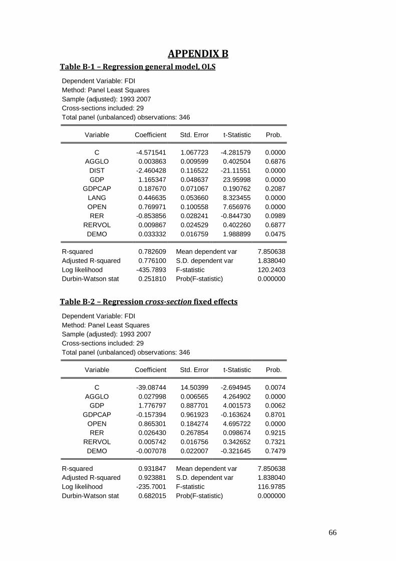
66
APPENDIX B Table B-1 – Regression general model, OLS
Dependent Variable: FDI
Method: Panel Least Squares
Sample (adjusted): 1993 2007
Cross-sections included: 29
Total panel (unbalanced) observations: 346
Variable Coefficient Std. Error t-Statistic Prob.
C -4.571541 1.067723 -4.281579 0.0000
AGGLO 0.003863 0.009599 0.402504 0.6876
DIST -2.460428 0.116522 -21.11551 0.0000
GDP 1.165347 0.048637 23.95998 0.0000
GDPCAP 0.187670 0.071067 0.190762 0.2087
LANG 0.446635 0.053660 8.323455 0.0000
OPEN 0.769971 0.100558 7.656976 0.0000
RER -0.853856 0.028241 -0.844730 0.0989
RERVOL 0.009867 0.024529 0.402260 0.6877
DEMO 0.033332 0.016759 1.988899 0.0475
R-squared 0.782609 Mean dependent var 7.850638
Adjusted R-squared 0.776100 S.D. dependent var 1.838040
Log likelihood -435.7893 F-statistic 120.2403
Durbin-Watson stat 0.251810 Prob(F-statistic) 0.000000
Table B-2 – Regression cross-section fixed effects
Dependent Variable: FDI
Method: Panel Least Squares
Sample (adjusted): 1993 2007
Cross-sections included: 29
Total panel (unbalanced) observations: 346
Variable Coefficient Std. Error t-Statistic Prob.
C -39.08744 14.50399 -2.694945 0.0074
AGGLO 0.027998 0.006565 4.264902 0.0000
GDP 1.776797 0.887701 4.001573 0.0062
GDPCAP -0.157394 0.961923 -0.163624 0.8701
OPEN 0.865301 0.184274 4.695722 0.0000
RER 0.026430 0.267854 0.098674 0.9215
RERVOL 0.005742 0.016756 0.342652 0.7321
DEMO -0.007078 0.022007 -0.321645 0.7479
R-squared 0.931847 Mean dependent var 7.850638
Adjusted R-squared 0.923881 S.D. dependent var 1.838040
Log likelihood -235.7001 F-statistic 116.9785
Durbin-Watson stat 0.682015 Prob(F-statistic) 0.000000

67
Table B-3 – Regression period fixed effects
Dependent Variable: FDI
Method: Panel Least Squares
Sample (adjusted): 1993 2007
Cross-sections included: 29
Total panel (unbalanced) observations: 346
Variable Coefficient Std. Error t-Statistic Prob.
C -9.788195 1.481721 -6.605964 0.0000
AGGLO -0.013138 0.015607 -0.841837 0.4005
GDP 0.559020 0.062964 8.878474 0.0000
GDPCAP 0.316310 0.105355 0.202329 0.8029
OPEN 0.657754 0.142640 1.905953 0.0696
RER -0.143553 0.030883 -4.648349 0.0000
RERVOL 0.037447 0.038439 0.974201 0.3307
DEMO -0.000349 0.024370 -0.014339 0.9886
R-squared 0.604664 Mean dependent var 7.850638
Adjusted R-squared 0.570821 S.D. dependent var 1.838040
Log likelihood -577.8500 F-statistic 14.91196
Durbin-Watson stat 0.123009 Prob(F-statistic) 0.000000
Table B-4 – Regression cross-section and period fixed effects
Dependent Variable: FDI
Method: Panel Least Squares
Sample (adjusted): 1993 2007
Cross-sections included: 29
Total panel (unbalanced) observations: 346
Variable Coefficient Std. Error t-Statistic Prob.
C -29.16287 12.97407 -5.330855 0.0000
AGGLO 0.014221 0.005254 2.706522 0.0072
GDP 1.480422 0.772728 3.515839 0.0001
GDPCAP 2.866639 0.874111 2.279490 0.7012
OPEN 0.743196 0.157085 3.911587 0.0027
RER -1.965144 0.396060 -4.961727 0.0000
RERVOL -0.003630 0.012880 -0.281835 0.7783
DEMO 0.001429 0.017148 0.083350 0.9336
R-squared 0.963508 Mean dependent var 7.850638
Adjusted R-squared 0.957302 S.D. dependent var 1.838040
Log likelihood -127.9458 F-statistic 155.2506
Durbin-Watson stat 0.901688 Prob(F-statistic) 0.000000

68
Table B-5 – Regression robust model (after EBA analysis)
Dependent Variable: FDI
Method: Panel Least Squares
Sample: 1992 2007
Cross-sections included: 32
Total panel (unbalanced) observations: 441
Variable Coefficient Std. Error t-Statistic Prob.
C -11.80753 1.139743 -10.35981 0.0000
GDP 0.661591 0.041118 16.09002 0.0000
OPEN 0.642358 0.079530 8.076970 0.0000
LANG 0.402703 0.042227 9.536579 0.0000
R-squared 0.539776 Mean dependent var 7.610377
Adjusted R-squared 0.535784 S.D. dependent var 1.918481
Log likelihood -756.3239 F-statistic 110.1616
Durbin-Watson stat 0.105151 Prob(F-statistic) 0.000000
Production costs robustness check
Table B-6 – Regression general model, OLS
Dependent Variable: FDI
Method: Panel Least Squares
Sample (adjusted): 1993 2007
Cross-sections included: 14
Total panel (unbalanced) observations: 197
Variable Coefficient Std. Error t-Statistic Prob.
C -6.306084 1.592302 -3.960357 0.0001
AGGLO 0.024254 0.009810 2.472349 0.0144
DIST -2.300908 0.147317 -15.61871 0.0000
GDP 1.290548 0.067081 19.23861 0.0000
LANG 0.078143 0.111562 1.700445 0.0086
OPEN 0.688378 0.147494 4.667166 0.0000
RER -0.305356 0.109760 -2.782025 0.0060
RERVOL -0.035264 0.029275 -1.204564 0.2300
DEMO 0.092836 0.050266 1.846902 0.0664
WAGE -0.007428 0.076603 -0.096965 0.9229
R-squared 0.834079 Mean dependent var 8.647526
Adjusted R-squared 0.824758 S.D. dependent var 1.884417
Log likelihood -217.6869 F-statistic 89.48000
Durbin-Watson stat 0.275907 Prob(F-statistic) 0.000000

69
Table B-7 – Regression cross-section fixed effects
Dependent Variable: FDI
Method: Panel Least Squares
Sample (adjusted): 1993 2007
Cross-sections included: 14
Total panel (unbalanced) observations: 197
Variable Coefficient Std. Error t-Statistic Prob.
C -48.07001 5.286443 -9.093073 0.0000
AGGLO 0.030923 0.006997 4.419238 0.0000
GDP 1.962846 0.240762 8.152647 0.0000
OPEN 0.436270 0.236689 1.843218 0.0671
RER 0.659184 0.541547 1.217224 0.2252
RERVOL 0.007263 0.020078 0.361754 0.7180
DEMO 0.164949 0.168028 0.981674 0.3277
WAGE 0.082270 0.366391 0.224541 0.8226
R-squared 0.935643 Mean dependent var 8.647526
Adjusted R-squared 0.927551 S.D. dependent var 1.884417
Log likelihood -128.1887 F-statistic 115.6150
Durbin-Watson stat 0.642471 Prob(F-statistic) 0.000000
Table B-8 – Regression period fixed effects
Dependent Variable: FDI
Method: Panel Least Squares
Sample (adjusted): 1993 2007
Cross-sections included: 14
Total panel (unbalanced) observations: 197
Variable Coefficient Std. Error t-Statistic Prob.
C -4.768916 2.313616 -1.196792 0.2331
AGGLO 0.046689 0.015167 3.078290 0.0024
GDP 0.519296 0.072709 7.142095 0.0000
OPEN 0.979021 0.183612 5.332003 0.0000
RER -0.641162 0.093932 -6.825790 0.0000
RERVOL -0.070290 0.042435 -5.656404 0.6995
DEMO 0.286739 0.049086 5.841579 0.0000
WAGE 0.260085 0.097131 0.677669 0.4082
R-squared 0.694169 Mean dependent var 8.647526
Adjusted R-squared 0.653637 S.D. dependent var 1.884417
Log likelihood -275.4758 F-statistic 17.12648
Durbin-Watson stat 0.336843 Prob(F-statistic) 0.000000

70
Table B-9 – Regression cross-section and period fixed effects
Dependent Variable: FDI
Method: Panel Least Squares
Sample (adjusted): 1993 2007
Cross-sections included: 14
Total panel (unbalanced) observations: 197
Variable Coefficient Std. Error t-Statistic Prob.
C -49.16392 14.32768 -3.431395 0.0008
AGGLO 0.014663 0.004897 2.994576 0.0032
GDP 1.479300 0.562224 2.631159 0.0094
OPEN 0.555378 0.173773 3.469602 0.0437
RER -0.355091 0.920503 -0.644844 0.0004
RERVOL 0.010122 0.013643 0.741905 0.4593
DEMO 0.065443 0.110805 0.590612 0.5557
WAGE 0.347484 0.333738 1.041185 0.2994
R-squared 0.975419 Mean dependent var 8.647526
Adjusted R-squared 0.969796 S.D. dependent var 1.884417
Log likelihood -37.23452 F-statistic 173.4683
Durbin-Watson stat 0.905879 Prob(F-statistic) 0.000000
Hausman tests
Table B-10 – Hausman test on cross-section random effects
Correlated Random Effects - Hausman Test
Equation: Untitled
Test cross-section random effects
Test Summary Chi-Sq. Statistic Chi-Sq. d.f. Prob.
Cross-section random 190.285418 7 0.0000
Table B-11 – Hausman test on period random effects
Correlated Random Effects - Hausman Test
Equation: Untitled
Test period random effects
Test Summary Chi-Sq. Statistic Chi-Sq. d.f. Prob.
Period random 23.909679 9 0.0044