the design of control architectures for force-controlled humanoids
TRANSCRIPT

The Design of Control Architectures
for Force-Controlled Humanoids
Performing Dynamic Tasks
Stuart O. Anderson
CMU-RI-TR-13-14
Submitted in partial fulfillment of the
requirements for the degree of
Doctor of Philosophy in Robotics
The Robotics Institute
Carnegie Mellon University
Pittsburgh, Pennsylvania 15213
May 2013
c© Copyright 2013 by Stuart O. Anderson. All Rights Reserved.

I certify that I have read this dissertation and that, in my opinion, it
is fully adequate in scope and quality as a dissertation for the degree
of Doctor of Philosophy.
(Jessica K. Hodgins) Principal Advisor
I certify that I have read this dissertation and that, in my opinion, it
is fully adequate in scope and quality as a dissertation for the degree
of Doctor of Philosophy.
(Christopher G. Atkeson)
I certify that I have read this dissertation and that, in my opinion, it
is fully adequate in scope and quality as a dissertation for the degree
of Doctor of Philosophy.
(Stefan Schaal (USC))
I certify that I have read this dissertation and that, in my opinion, it
is fully adequate in scope and quality as a dissertation for the degree
of Doctor of Philosophy.
(Hartmut Geyer)
ii

Approved for the University Committee on Graduate Studies
iii

Preface
This thesis is about improving the process of designing controllers for humanoid
robots. It describes tools we designed that enable us to iterate faster when experi-
menting with control systems that aggregate multiple model based sub-controllers.
Many model based humanoid controllers can be considered approximations to a
fully general, but computationally intractable, controller. Typically, simplified models
are used to make the control problem tractable, but must be well chosen to capture
the most important features of the problem domain. Because it is difficult to know
apriori which simplified representations will perform best, the ability to experiment
with different representations is an important feature of an effective controller design
workflow.
Control designs based on simplified state representations typically combine con-
trollers that solve specific sub-problems into a single aggregate controller. Common
examples include the aggregation of trajectory generators with trajectory trackers,
and balance controllers with end-effector force controllers. The primary contribution
of this thesis is a method for aggregating sub-controllers that automates constructing
models of the behavior of those sub-controllers. This method allows tight runtime cou-
pling between sub-controllers, while limiting the need to adjust several sub-controllers
to compensate for experimental changes made to any individual sub-controller. We
call this combination of tightly coupled sub-controllers with automated model build-
ing Informed Priority Control.
We describe the application of Informed Priority Control to humanoid balance
tasks, including the bongo-board balance task, and show experimental results in both
simulation and hardware environments. We produced stable controllers for simple
iv

balance tasks in both environments, but were only able to demonstrate robust con-
trollers for the more difficult bongo-board task in simulation. We include an analysis
of the instability of the bongo-board controller in hardware, focusing on the role of
unmodeled sensor dynamics.
v

Acknowledgments
The author wishes to thank Dr. Jessica K. Hodgins, who advised the research and
writing of this thesis, and without whose expertise, wisdom, support and patience
this work could not have succeeded. Dr. Christopher G. Atkeson was an invaluable
source of sage advice and discussion throughout the course of this work. Additional
thanks are due to the author’s unerringly supportive parents, and of course, to the
red-shoed robot’s first namesake, Dorothy Haffey.
Financial support was provided by NSF Grants CNS-0224419, DGE-0333420,
ECS-0325383, and EEC-0540865.
vi
Contents
Preface iv
Acknowledgments vi
1 Introduction 1
1.1 Example Tasks . . . . . . . . . . . . . . . . . . . . . . . . . . . . . . 5
2 Related Research 10
2.1 The Humanoid Form . . . . . . . . . . . . . . . . . . . . . . . . . . . 10
2.1.1 Aggregate Controllers and Simplified Models . . . . . . . . . . 11
2.1.2 Joint Torque Control . . . . . . . . . . . . . . . . . . . . . . . 20
2.1.3 Modeling and Sensing Errors . . . . . . . . . . . . . . . . . . . 21
3 Simplified Models 24
3.1 Related Model Reduction Research . . . . . . . . . . . . . . . . . . . 26
3.2 Notation . . . . . . . . . . . . . . . . . . . . . . . . . . . . . . . . . . 29
3.2.1 System Representation . . . . . . . . . . . . . . . . . . . . . . 29
3.2.2 Control Representation . . . . . . . . . . . . . . . . . . . . . . 30
3.3 Approximation Error in Simplified Models . . . . . . . . . . . . . . . 31
3.3.1 Computational Difficulties . . . . . . . . . . . . . . . . . . . . 33
3.3.2 Selecting Features . . . . . . . . . . . . . . . . . . . . . . . . . 34
3.3.3 Selecting Benign Actions . . . . . . . . . . . . . . . . . . . . . 34
3.4 Automated Model Reduction . . . . . . . . . . . . . . . . . . . . . . 36
3.5 Automatic Generation of Linear Models . . . . . . . . . . . . . . . . 38
vii

3.6 Automatic Generation of Reduced Models . . . . . . . . . . . . . . . 39
3.6.1 Linear Models . . . . . . . . . . . . . . . . . . . . . . . . . . . 39
3.6.2 Nonlinear Models . . . . . . . . . . . . . . . . . . . . . . . . . 41
3.6.3 Relation to Generalized Coordinates and Lagrangian Dynamics 45
3.7 Bongo-Board Reduced Model Design . . . . . . . . . . . . . . . . . . 47
3.7.1 Action Space Selection . . . . . . . . . . . . . . . . . . . . . . 49
4 Controller Architecture 53
4.1 Related Research in Humanoid Robot Control . . . . . . . . . . . . . 58
4.2 Trajectory Optimization . . . . . . . . . . . . . . . . . . . . . . . . . 60
4.3 Policy Mixing Control Framework . . . . . . . . . . . . . . . . . . . . 63
4.3.1 Dynamics . . . . . . . . . . . . . . . . . . . . . . . . . . . . . 64
4.3.2 Policy Mixing . . . . . . . . . . . . . . . . . . . . . . . . . . . 64
4.3.3 Policy mixing . . . . . . . . . . . . . . . . . . . . . . . . . . . 65
4.4 Implementation . . . . . . . . . . . . . . . . . . . . . . . . . . . . . . 65
4.4.1 Lumped mass policy . . . . . . . . . . . . . . . . . . . . . . . 66
4.4.2 Body posture policy . . . . . . . . . . . . . . . . . . . . . . . 67
4.4.3 Static contact load policies . . . . . . . . . . . . . . . . . . . . 68
4.4.4 Solving for Desired Torques . . . . . . . . . . . . . . . . . . . 69
4.5 Informed Priority Control . . . . . . . . . . . . . . . . . . . . . . . . 69
4.5.1 Informed Priority Control Framework . . . . . . . . . . . . . . 71
4.6 Implementation of Informed Priority Control . . . . . . . . . . . . . . 74
4.6.1 Base Policy . . . . . . . . . . . . . . . . . . . . . . . . . . . . 74
4.7 Linear Feedback Component . . . . . . . . . . . . . . . . . . . . . . . 76
4.8 Gravity Compensation Component . . . . . . . . . . . . . . . . . . . 81
4.9 Enforcing Output Constraints . . . . . . . . . . . . . . . . . . . . . . 83
4.10 Receding Horizon Control . . . . . . . . . . . . . . . . . . . . . . . . 84
4.10.1 System Models for Receding Horizon Control . . . . . . . . . . 86
4.11 Mode Switching Control . . . . . . . . . . . . . . . . . . . . . . . . . 87
4.12 Summary . . . . . . . . . . . . . . . . . . . . . . . . . . . . . . . . . 90
viii

5 Modeling and Sensing Error 91
5.1 Kinematic Calibration . . . . . . . . . . . . . . . . . . . . . . . . . . 91
5.1.1 Initial Calibration . . . . . . . . . . . . . . . . . . . . . . . . . 92
5.1.2 On-line kinematic recalibration . . . . . . . . . . . . . . . . . 92
5.2 Load Calibration . . . . . . . . . . . . . . . . . . . . . . . . . . . . . 94
5.2.1 Joint load sensors . . . . . . . . . . . . . . . . . . . . . . . . . 94
5.2.2 Foot load sensors . . . . . . . . . . . . . . . . . . . . . . . . . 95
5.3 Model Identification . . . . . . . . . . . . . . . . . . . . . . . . . . . 96
5.4 Model Adaptation . . . . . . . . . . . . . . . . . . . . . . . . . . . . 97
5.4.1 Full model . . . . . . . . . . . . . . . . . . . . . . . . . . . . . 98
5.4.2 Simplified models . . . . . . . . . . . . . . . . . . . . . . . . . 100
6 Experimental Results 102
6.1 Seesaw Balance . . . . . . . . . . . . . . . . . . . . . . . . . . . . . . 102
6.1.1 Experimental Setup . . . . . . . . . . . . . . . . . . . . . . . . 103
6.1.2 Trials . . . . . . . . . . . . . . . . . . . . . . . . . . . . . . . 103
6.1.3 Discussion . . . . . . . . . . . . . . . . . . . . . . . . . . . . . 104
6.2 Bongo-Board Balance . . . . . . . . . . . . . . . . . . . . . . . . . . . 110
6.2.1 Bongo-Board Simulation . . . . . . . . . . . . . . . . . . . . . 110
6.3 Results . . . . . . . . . . . . . . . . . . . . . . . . . . . . . . . . . . . 111
6.3.1 Mode Switching Control . . . . . . . . . . . . . . . . . . . . . 114
6.4 Failure Analysis . . . . . . . . . . . . . . . . . . . . . . . . . . . . . . 117
6.4.1 Discussion . . . . . . . . . . . . . . . . . . . . . . . . . . . . . 138
7 Conclusions 143
ix

List of Tables
3.1 Reduced Models . . . . . . . . . . . . . . . . . . . . . . . . . . . . . . 47
3.2 Bongo-board Eigenvectors . . . . . . . . . . . . . . . . . . . . . . . . 49
4.1 Sub-policy relationships . . . . . . . . . . . . . . . . . . . . . . . . . 55
6.1 Decision Surface Parameters . . . . . . . . . . . . . . . . . . . . . . . 116
x
List of Figures
1.1 Sarcos Primus Biped. . . . . . . . . . . . . . . . . . . . . . . . . . . . 6
1.2 The Sarcos Primus humanoid on a seesaw. . . . . . . . . . . . . . . . 7
1.3 The Sarcos Primus humanoid on a bongo-board. . . . . . . . . . . . . 8
3.1 Reduced model design processes . . . . . . . . . . . . . . . . . . . . . 37
3.2 Alterations to finite difference for model reduction . . . . . . . . . . . 40
3.3 Lumped-mass accelerations . . . . . . . . . . . . . . . . . . . . . . . . 46
3.4 Reduced models of the bongo-board . . . . . . . . . . . . . . . . . . . 48
3.5 Bongo-board kinematics . . . . . . . . . . . . . . . . . . . . . . . . . 49
3.6 Bongo-board action space . . . . . . . . . . . . . . . . . . . . . . . . 51
3.7 Bongo-board eigenvectors . . . . . . . . . . . . . . . . . . . . . . . . 52
3.8 Orthogonal Torques . . . . . . . . . . . . . . . . . . . . . . . . . . . . 52
4.1 Software architectures . . . . . . . . . . . . . . . . . . . . . . . . . . 54
4.2 The reduced lumped mass seesaw model . . . . . . . . . . . . . . . . 67
4.3 Simulated biped performing bongo-board balance task . . . . . . . . 71
4.4 Policy Mixing and Informed Priority Control . . . . . . . . . . . . . . 72
4.5 Control architecture implementations . . . . . . . . . . . . . . . . . . 73
4.6 Control flow diagram for task and base policy . . . . . . . . . . . . . 76
4.7 Oscillation during gain tuning . . . . . . . . . . . . . . . . . . . . . . 80
4.8 Underdetermined gravity compensation . . . . . . . . . . . . . . . . . 82
4.9 Sequence of optimization steps in the bongo-board controller . . . . . 83
4.10 Hybrid Linear Dynamics . . . . . . . . . . . . . . . . . . . . . . . . . 88
xi

5.1 Foot accelerations . . . . . . . . . . . . . . . . . . . . . . . . . . . . . 93
5.2 Methods for applying test torques . . . . . . . . . . . . . . . . . . . . 95
5.3 Mass model fit . . . . . . . . . . . . . . . . . . . . . . . . . . . . . . 97
6.1 Policy dominance . . . . . . . . . . . . . . . . . . . . . . . . . . . . . 107
6.2 Model adjustment during trial without external disturbance. . . . . . 108
6.3 Model adjustment during external disturbance. . . . . . . . . . . . . 109
6.4 Bongo-board angle . . . . . . . . . . . . . . . . . . . . . . . . . . . . 112
6.5 Bongo-board model robustness . . . . . . . . . . . . . . . . . . . . . . 113
6.6 Bongo-board mass error robustness . . . . . . . . . . . . . . . . . . . 115
6.7 High Frequency Failure (State) . . . . . . . . . . . . . . . . . . . . . 119
6.8 High Frequency Failure (Action) . . . . . . . . . . . . . . . . . . . . . 120
6.9 Bang-Bang Failure (State) . . . . . . . . . . . . . . . . . . . . . . . . 121
6.10 Bang-Bang Failure (Action) . . . . . . . . . . . . . . . . . . . . . . . 122
6.11 Increasing Oscillation Failure (State) . . . . . . . . . . . . . . . . . . 123
6.12 Increasing Oscillation Failure (Action) . . . . . . . . . . . . . . . . . 124
6.13 Action Transient . . . . . . . . . . . . . . . . . . . . . . . . . . . . . 125
6.14 Action Transient Velocity . . . . . . . . . . . . . . . . . . . . . . . . 126
6.15 Gain Response . . . . . . . . . . . . . . . . . . . . . . . . . . . . . . 127
6.16 Gain Trials . . . . . . . . . . . . . . . . . . . . . . . . . . . . . . . . 129
6.17 Gain Trials Actions . . . . . . . . . . . . . . . . . . . . . . . . . . . . 130
6.18 Hardware to simulation failure state comparison . . . . . . . . . . . . 131
6.19 Hardware to simulation failure action comparison . . . . . . . . . . . 132
6.20 Signal Delay Trials State . . . . . . . . . . . . . . . . . . . . . . . . . 133
6.21 Signal Delay Trials Velocity . . . . . . . . . . . . . . . . . . . . . . . 134
6.22 Contact Model Trials State . . . . . . . . . . . . . . . . . . . . . . . . 136
6.23 Contact Model Trials Action . . . . . . . . . . . . . . . . . . . . . . . 137
6.24 Force Plate Sensor Traces . . . . . . . . . . . . . . . . . . . . . . . . 139
6.25 Force Plate Sensor Error . . . . . . . . . . . . . . . . . . . . . . . . . 140
xii

Chapter 1
Introduction
The design and implementation of control systems for humanoid robots presents a
combination of challenges not encountered elsewhere in robotics literature. Principal
among these challenges are the large number of unique degrees of freedom and control
inputs, the difficulty of building accurate physical models of these systems, and the
complex contact between the robot and its environment encountered during dynamic
balancing. Extensive research during the past forty years has resulted in methods
for designing controllers that meet these challenges for specific tasks, with varying
degrees of success. Among these existing methods, we are particularly interested in
the model based optimal control framework. This framework can be applied naturally
to a wide variety of tasks, and is already well studied in other areas of robotics.
Within the model based optimal control framework, it is widely accepted that
tractable solutions for humanoid robots require the use of heuristics and simplifica-
tions based on domain knowledge. We consider two broad categories of simplifica-
tions: first, the use of approximate models to reduce dimensionality and second, the
division of a complex control task into simpler tasks, each performed by an indepen-
dent sub-controller. These simplifications are approximations that carry a cost, paid
in suboptimal performance and lost stability guarantees. While it is not surprising
that the fundamentally hard problem of designing an optimal policy for a nonlinear
time-invariant system cannot be solved practically except in approximation, there
are surprising differences between the performance of controllers based on the various
1

CHAPTER 1. INTRODUCTION 2
approximations. This thesis investigates both categories of simplification made in the
design of controllers for humanoid robots, and the impact these approximations have
on system performance.
The central contribution of this thesis, Informed Priority Control, is a method for
constructing a humanoid control system that aggregates model based sub-controllers.
Informed Priority Control is distinguished by its ability to build new models of sub-
controller behavior after every configuration change. These models allow model based
sub-controllers to automatically adapt to configuration changes made to other sub-
controllers, while still using a cascade style control architecture that tightly couples
controller outputs. In this way, Informed Priority Control provides tight run-time
coupling of sub-controllers, while de-coupling configuration-time changes made to
individual controllers. This combination of properties permits rapid experimenta-
tion with simplified model representations and other configuration-time parameters,
because changes to one sub-controller do not require reciprocal changes to other com-
ponents.
Other control designs also permit this decoupling between sub-tasks, but that de-
coupling is often achieved by enforcing a run-time separation into independent modes
or subspaces. This decoupling can be difficult to achieve when tasks are sensitive to
model error. Other existing designs that do not employ this type of stiff run-time
decoupling, such as those based on behavioral primitives or trajectory tracking, intro-
duce configuration-time dependencies between sub-policies. For example, because of
these dependencies, when a behavioral primitive is altered, any policies that employ
that primitive may need to be updated to reflect that alteration.
The primary design goal of Informed Priority Control is to allow rapid experimen-
tation with different simplified models. Model simplification is widely used because
the computational complexity of many model based controllers is tied strongly to
the dimensionality of the system model they operate on. Model reduction decreases
these computational costs by creating simplified approximations to complex system
models. The performance of a controller using a simplified model, relative to one us-
ing the corresponding full model, depends on the relationship between the task being
performed and the model simplification used. Because this relationship is complex,

CHAPTER 1. INTRODUCTION 3
efficient experimentation and iteration are important properties of an effective control
design methodology.
One example of the complexity of this relationship occurs when decoupling the
coronal and sagittal plane dynamics of the body, a common choice for simplified
models of humanoid standing balance. For some tasks, the error introduced by this
simplification is small. However, controllers that use these models can have difficulty
when the behaviors needed to complete the task require significant angular momentum
and a body configuration in which the axes of the inertia ellipse are not aligned to
the sagittal and coronal planes. For these tasks, the use of these decoupled models
may significantly reduce performance because the dynamic coupling between the two
planes is not captured in the control design process.
Similarly, if a simplified model represents only the robot’s angular momentum,
the joint accelerations required to achieve a specific change in that momentum are
determined by the current joint angles. If an optimal controller uses the simplified
model state as the input to its objective function, it cannot accurately model joint
accelerations or total kinetic energy. For example, when the knee joints are near a
singularity, some changes in total system momentum may be possible but require
very high knee acceleration to achieve. Because the current joint angles are not fully
captured by the simplified model’s state, a controller using that simplified model may
select actions that result in undesirable joint accelerations.
Likewise, the lack of a knee joint in some sagittal models can have similar effects,
restricting the space of control results to those that do not require knee motions.
Some models, like SLIP [Alexander, 1992], use a telescoping joint to approximate a
rotational knee joint. However, even this approximation does not capture the range
of motion limits and the dependence of the end effector Jacobian on knee angle that a
rotational knee introduces. Additionally, some controllers and design methodologies
are more sensitive to errors in sensor calibration and model parameters than others.
The automatic model reduction techniques we introduce in this thesis make it
feasible to rapidly iterate the design of the reduced model component of a larger
control framework, making it easier to explore which features are important for a given
task, and which models are robust to model parameter error. How well these simplified

CHAPTER 1. INTRODUCTION 4
models approximate the salient features of the full model, and the performance impact
of this approximation are the focus of Chapter 3.
Informed Priority Control specifies how the sub-controllers used to construct a task
solution are combined. By separating a control problem into discrete stages, such that
the outputs of these stages are independent, overall computational complexity can
be reduced significantly. However, when the parts of the problem solved in each of
these stages are not truly independent, assuming their independence may result in
sub-optimal performance.
One example occurs in the design of trajectory tracking zero moment point con-
trollers [Kajita et al., 2003]. In this framework the trajectory planner and trajectory
tracker are designed independently. Because performance depends on the relationship
between the tracker and the trajectory it tracks, optimizing the performance of the
aggregate system requires that both the trajectory and its tracker be optimized simul-
taneously. Similarly, when a sub-controller’s output is expressed in a low dimensional
space and used as an input to a lower-level controller, it may not be able to express
the optimal actions for its task in the input space of that lower-level controller.
In Chapter 4, we examine several control frameworks and the problems that can
result from their implicit decoupling of sub-tasks, then describe Informed Priority
Control, and its predecessor in our work, Policy Mixing Control, which attempt to
mitigate some of these effects.
Both these types of simplifications can influence a controller’s sensitivity to un-
modeled differences between the physical system and the full model of the system,
as well as its sensitivity to incomplete or inaccurate sensing of the system state. For
example, the Sarcos humanoid has a stiff hydraulic umbilical that applies forces on
the order of 25N to the robot’s hip during standing balance tasks. These unmodeled
disturbances can significantly affect the performance of controllers that are unable
to compensate for them. Model and sensor error, and methods that can be used to
mitigate them, are addressed in Chapter 5.
In Chapter 6 we describe the results of our experiments with policy mixing control
and its successor, informed priority control. With policy mixing control we were able
to demonstrate stable behavior on our seesaw-push task both in simulation and on

CHAPTER 1. INTRODUCTION 5
the physical hardware. The informed priority controller was able to complete the
bongo-board task in simulation, but we were unable to demonstrate stable perfor-
mance using the hardware. We provide an analysis and additional experimental data
investigating why the controller was unable to stabilize the system, focusing on the
role of systematic errors in sensing the position of the bongo-board roller caused by
unmodeled sensor dynamics.
This thesis describes contributions to the existing literature in humanoid robotics.
The primary contribution made by this thesis is the Informed Priority Control
framework (Section 4.5), and the Automatic Model Reduction method (Sec-
tion 3.4) that permits its practical implementation. An additional minor contribu-
tions is the Minimum Variance Gravity Compensation (Section 4.8) technique
used to build the robust base policy for our informed priority controller. It is gener-
ally applicable in the context of humanoid controllers. Finally, the Time-Coupled
Minimax dynamic programming technique (Section 4.11) used in designing a mode
switching controller that is robust to sensor error extends existing work in designing
robust model based policies.
1.1 Example Tasks
This thesis discusses controllers for two tasks performed by the Sarcos Primus hu-
manoid. These tasks are balance on a seesaw, and balance on a bongo-board. In our
earlier work we also describe controllers for standing balance, forward walking, and
motion capture playback [Anderson et al., 2006, 2007]. The primary contributions
presented in this thesis were demonstrated in the context of the seesaw and bongo-
board balance tasks. This section describes the Sarcos Primus biped, and the tasks
we studied with it.
The experimental platform for this work was the Sarcos Primus biped shown
in figure 1.1. The Sarcos Primus is a 1.6 meter tall humanoid robot that weighs
approximately 92 kilograms. It has 34 hydraulically actuated joints, seven in each
limb, three in the trunk, and an additional three in the neck. Each joint is equipped
with a position sensor and a load cell, and each foot contains a six axis load sensor. A

CHAPTER 1. INTRODUCTION 6
Figure 1.1: Sarcos Primus Biped.
five kHz local control loop allows compliant force control of all joints. In addition to
the per-joint load cells each foot is equipped with a six-axis load cell. A Microstrain
3DM-GX3 IMU [Microstrain, Inc., 2008] attached to the robot’s chest provided global
orientation information.
The seesaw balance task required the Sarcos humanoid to balance on a plank
supported by a rotational joint (figure 1.2). The robot’s feet were located at opposite
ends of the plank, and the rotational joint was positioned in the middle of the plank.
We built the small seesaw using a board mounted on bearings with a total range of
motion of 20 degrees from side to side. The task began with one end of the plank in
contact with the ground. Then, the robot shifted its weight so that the opposite end
of the plank came into contact with the ground. During the course of a single trial the
robot shifted its weight to alternate which end of the board was in contact with the
ground several times. In some trials, the robot was also pushed by the experimenter

CHAPTER 1. INTRODUCTION 7
Figure 1.2: The Sarcos Primus humanoid on a seesaw.
so that the end of the plank left the ground unexpectedly.
The seesaw task is difficult because changes in contact state are hard to predict. In
particular, the impact between the end of the board and the ground can easily cause
the foot on the end of the board opposite the impact to lose contact with the board.
Absorbing the shock of this impact requires that the robot adjust its impedance in
anticipation of the impact event. Other researchers have also studied the seesaw
balance task, and found the same principal sources of difficulty [Hyon, 2009].
The bongo-board task requires the robot to maintain its balance on a circus prop
known as a rola-bola or bongo-board. A bongo-board consists of a long cylinder that
is free to roll on the ground, and a plank placed on top of that cylinder. The cylinder
does not slip with respect to either the ground or the plank. The performer stands
on the plank and balances without allowing the plank to contact the ground, or roll

CHAPTER 1. INTRODUCTION 8
Figure 1.3: The Sarcos Primus humanoid on a bongo-board.
off the end of the cylinder. The experimental setup used for the bongo-board balance
task is shown in figure 1.3.
Both the seesaw and bongo-board tasks have underactuated degrees of freedom
that are sensitive to large forces. In the seesaw task both the seesaw itself and the
unilateral foot contact constraints have this property, and in the bongo-board task the
low-mass bongo-board sub-system has this property. In both tasks, it can be difficult
to avoid applying large forces to these degrees of freedom if the robot is controlled by
a stiff postural controller.
In the seesaw task the forces applied to the robot by the seesaw change rapidly
as the end of the board comes into contact with the ground, and can cause one or
both of the feet to lose contact with the board. In the bongo-board task the ability
to rapidly shift the position of the roller depends on that motion not being coupled to

CHAPTER 1. INTRODUCTION 9
accelerations in the position of the robot’s center of mass. Errors in state estimation
can result in large center of mass accelerations during position tracking.
The seesaw task benefits from compliance with the impact forces that occur when
an end of the seesaw hits the ground. The bongo-board task does not include impact
forces, but is simplified if the robot is able to comply with the board-roller system
as it drives the board to a desired angle and position. Controlling the board angle
requires compliance because the board-roller contact point is not precisely known
and can change rapidly. The motion of each foot relative to the robot’s center of
mass that is needed to change the board angle is determined by the kinematics of the
board-roller contact point. This constraint motivates controlling board angle through
compliant force control rather than stiff position control.
Chapter 6 discusses these tasks, and the performance of our controllers when
applied to these tasks.

Chapter 2
Related Research
This chapter provides a broad overview of the context within which the research
described in this thesis was conducted. More specific discussion of research related to
the generation and application of simplified models is included in chapter 3. Likewise,
discussion of research related to our work in control architecture design is discussed
in chapter 4.
A central theme in the humanoid robotics literature is the need to resolve diffi-
culties associated with the humanoid form. The first section of this chapter discusses
these difficulties and the range of existing approaches to resolving them. A secondary
theme that plays an important role in our work is the need for methods that produce
accurate models of the physical robot hardware, and compensate for residual inaccu-
racies in those models. The second section of this chapter discusses model fitting and
model error adaptation techniques related to those we employ.
2.1 The Humanoid Form
There are many reasons to build a robot with a humanoid form. These include the
ability to navigate and manipulate the built environment effectively, the availability of
example motion collected from humans, and the human social response to humanoid
agents [Mutlu et al., 2009]. However, the humanoid form also presents unique chal-
lenges. These include the large number of degrees of freedom, the limited base of
10

CHAPTER 2. RELATED RESEARCH 11
support, redundant degrees of freedom, and the need for low impedance controllers in
unknown environments. This section discusses existing approaches to meeting each
of these challenges.
The challenges most central to the work in this thesis are those presented by the
large number of degrees of freedom required for a humanoid robot. These challenges
have been widely studied in the robotics literature, as well as the graphics literature
related to animating humanoid characters. Because these research communities share
many techniques, we organize our discussion of related work primarily by properties
of the approach, rather than by the application domain.
2.1.1 Aggregate Controllers and Simplified Models
A common approach when developing control policies for humanoids is to decompose
a task into subtasks that are individually less difficult to solve. How a task is decom-
posed into sub-controllers and how these sub-controllers are aggregated to produce
a solution is an important property of a control approach. Methods like state space
funnels [Mason, 1985, Erdmann and Mason, 1988], behavioral primitives [Mataric
et al., 1998, Fod et al., 2002, Jenkins and Mataric, 2003], hybrid systems [Branicky
et al., 2000], and reinforcement learning based on behavioral primitives [Bentivegna
and Atkeson, 2001] are all variations of this basic divide and conquer approach. In
practice, finding a useful decomposition is often not automated and relies heavily on
expert human knowledge of a particular problem domain.
Control decompositions often take one of two forms, serial decomposition and
parallel decomposition. Controllers that combine these forms are also possible. Serial
decomposition of a control problem involves separating it into stages, arranged from
low level behavioral controllers to high level task controllers. Each stage’s control
output is treated as the control input to the next stage, and in this way a chain
of linked controllers is built. Parallel decomposition involves decomposing a complex
problem into multiple tasks that share a single control output space, such as a posture
controller that moves an end effector and a balance controller that controls center of
mass. These controllers have control outputs in non-orthogonal subspaces of the space

CHAPTER 2. RELATED RESEARCH 12
of joint torques.
Most approaches to generating motion for humanoids, including ours, make exten-
sive use of simplified models of the humanoid. Single lumped mass models are among
the most intuitive and analytically tractable of these simplified models. Researchers
have recognized that stabilizing the center of mass while respecting the constraints
imposed by the small foot contact region is often the principal challenge when bal-
ancing [Garcia et al., 1998, Goswami et al., 1996, M. Vukobratovic and B. Borovac,
2004]. Because the motion of the center of mass is fully determined by the ground
contact forces, some researchers have developed algorithms for transforming a desired
center of mass acceleration into foot contact loads, then expanding those contact loads
into joint torques [Stephens, 2010, Hyon et al., 2007]. These methods fully determine
the contact forces before considering the desired actions of other component policies,
creating a strict priority ordering of control objectives.
For example, the serial decomposition based Dynamic Balance Force Control
(DBFC) controller described in chapter five of Stephens’ thesis [Stephens, 2011] con-
structs ground contact forces in two steps. First, a space of possible contact forces
that produce desired momentum changes given expected external disturbance forces
is computed. These desired momentum changes can be computed quickly by optimiz-
ing control actions over the simplified model. After the desired momentum change is
chosen, joint torques that produce these momentum changes are computed. The first
step, because it determines the total change in system momentum, must also deter-
mines the aggregate ground contact force. This strict priority ordering is required to
extend the stability properties of the controller operating on the single mass system
to the aggregate controller operating on the full body. Only if the desired aggregate
ground contact forces produced by reduced model controller are unmodified by higher
level controllers is it possible to argue that the center of mass of the full system will
be stabilized because the center of mass of the reduced system is stabilized.
In contrast, the null space control methods introduced by Sentis and Khatib [2006]
use a parallel decomposition structure to design stable controllers, but are often used
with more complex, multi-body, approximate models. These methods combine several
controllers with non-orthogonal output spaces. The highest priority controller, often
CHAPTER 2. RELATED RESEARCH 13
a balance control task, produces a low dimensional control output, often an aggregate
ground contact force or center of mass motion. The control action of the controller
with second highest priority is projected into the null space of the first controller’s
output space, ensuring that the combined control action, when projected into the
control space of the balance task, is unaltered. This process continues until all control
actions have been combined. This process allows researchers to produce controllers
for essential tasks like maintaining balance only once. Then, task-specific controllers
can later be added to control end effector position of body posture without the risk
of altering the more important balance behavior.
While the ability to reason about the stability of the aggregate system based on the
stability of the sub-controllers delivered by a strict priority ordering is desirable, there
are two potential problems with this approach that we have tried to address in our
work. First, when two control policies with very different impedances are combined in
orthogonal subspaces, the aggregate controller can exhibit chattering behavior. This
behavior occurs because the impedance mismatch between the controllers creates an
aggregate controller with a long narrow impedance ellipse. In our early work with
policy mixing control designs [Anderson and Hodgins, 2010], we combined a desired
contact load with other control objectives to produce desired joint torques in a single
operation, taking into account the desired actions of all policies simultaneously. This
approach is similar to the null space control methods described by Sentis and Khatib,
but relaxes the null space constraint into a weighted optimization problem. The intent
was to regularize the impedance of the aggregate policy to improve stability.
The second problem with strict priority order approaches that our work attempts
to resolve is that there is no explicit exchange of information between sub-controllers
about their future control outputs. For example, a high priority balance controller
may plan a series of ground reaction forces that maintain balance when faced with
a non-minimum phases balance task. If a lower priority pose controller is unaware
of the high priority controller’s future plans it may drive the system to a configura-
tion (i.e. fully extended knees) where the desired ground reaction forces cannot be
achieved, destabilizing the aggregate controller. Alternately, if the desired pose is a
function of the current center of mass, the system may oscillate in the null space of
CHAPTER 2. RELATED RESEARCH 14
center of mass motion. This oscillation occurs when the bandwidth of the posture
and balance controllers are mismatched. Informed Priority control shares models of
sub-controller behavior between sub-controllers so that model based sub-controllers
can optimize their behavior based on knowledge of how other, lower priority, sub-
controllers will behave. Specifically, information about the impedance of the con-
nected sub-controllers is captured and provided in the form of a sub-system model.
In the case of Informed Priority control this information sharing is achieved without
relaxing the stability guarantees provided by priority based control methods.
A unicycle controller developed by Vos [1990] demonstrated two techniques for
coupling sub-controllers that were influential in our work. First, the coupling of lateral
and longitudinal controllers through gain scheduling based on the open loop dynamics
of wheel speed is similar to our use of open loop models of sub-controllers. Our interest
in this type of dynamic coupling was specifically influenced as well by Whitman’s
work on dynamic programming [Whitman and Atkeson, 2010] using instantaneously
coupled policies. The second technique from Vos’s work was the use of inner and
outer loop controllers in the longitudinal controller. The use of the inner loop’s open
loop transfer function in designing the outer loop’s Kalman filter gains was influential
in our development of the model sharing feature of Informed Priority Control.
State Machines
One increasingly popular method of aggregating sub-controllers relies on finite state
machines to transition between a set of simple control policies. These controllers are
especially appropriate for tasks with distinct phases like walking, running, or jumping.
The hybrid linear mode switching controller we discuss in section 4.11 provides an
example of this type of policy applied to bongo-board balance.
The SIMBICON controller developed by Yin and colleagues [Yin et al., 2007] pro-
duced robust two and three dimensional behavior for a simulated humanoid. The
authors show that its motions can be tuned automatically from human motion cap-
ture data. The controller design is similar to earlier work [Raibert, 1986, Anderson
et al., 2005], in that it uses a finite state machine to transition between target poses,
controls some link orientations with respect to the world frame, and achieves robust

CHAPTER 2. RELATED RESEARCH 15
performance using tuned linear feedback. The work was novel because it produced a
large variety of behaviors in two and three dimensions, presented a method for semi-
automatically altering controllers based on motion capture data, and used feedback
error learning to generate feedforward torques.
The state machine transitions between desired poses on foot contact or after fixed
time intervals. The swing leg femur orientation and the torso orientation are con-
trolled relative to world coordinates. Linear feedback is used to continuously vary
desired joint angles, often the swing leg hip and stance ankle, as a function of center
of mass position (relative to the stance ankle) and velocity. Motion capture data is
used to design controllers by using Fourier analysis to extract a periodic movement.
That periodic movement is then tracked, with the phase of the tracking being reset
on foot contact. Finally, feedback error learning is used to improve the behavior of
the system over time and permit better performance with lower gains. The particu-
lar feedback error learning method employed computes the feedforward torque as a
function of gait phase.
More recent work by Wang and colleagues extends the SIMBICON controller to
make it more robust by optimizing its parameters over many trials [Wang et al., 2009].
This work uses the covariance matrix adaptation method [Hansen and Ostermeier,
1996] to optimize the gait parameters. Covariance matrix optimization is a derivative
free optimization method that maintains a Gaussian distribution from which new test
points are drawn, and updates this distribution based on the value of the objective
function at those points. This approach allows it to make efficient use of samples,
an important property when evaluating the objective function is computationally
expensive, as it is in this case. In their later work, by optimizing in conditions where
unexpected disturbances are applied, the authors are able to generate more robust
controllers [Wang et al., 2010]. Finally, their most recent work showed that natural
and robust gait could be generated using simple models of human muscle and tendon
to drive the primary degrees of freedom, and optimizing per-muscle force and length
feedback parameters as well as trajectory tracking gains and desired poses [Wang
et al., 2012]. The resulting gait controller can be parameterized in fifty six parameters,
making direct optimization of those parameters feasible.

CHAPTER 2. RELATED RESEARCH 16
Sampling Based Methods
Sampling-based dynamic programming [Atkeson and Stephens, 2007, Atkeson and
Morimoto, 2003] and rapidly exploring random trees [LaValle, 1998] use random
sampling of states to find policies or trajectories in high dimensional spaces. Be-
cause trajectory optimization is tractable in high dimensional systems, it can be used
as a building block to construct trajectory-based controllers. These control methods
do not aggregate sub-controllers, but attempt to find a policy in the full state space
by exploring that space efficiently.
Sampling-based dynamic programming builds a locally linear policy and locally
quadratic value function incrementally using trajectory optimization. The process
iteratively improves an approximate policy and value function. At each iteration, a
random point is selected and the current policy is used to compute an initial trajec-
tory that is then refined by differential dynamic programming (DDP). The new value
function approximation at the initial point, based on the newly optimized trajectory,
is added to the value function approximation if the local approximation differs sig-
nificantly from the prior value function at that point. The empirical value of the
randomly sampled state is computed from this refined trajectory. If the expected
value and true value differ significantly then the linear policy and quadratic value
function approximation at the new point are added to the global policy. Each initial
point is selected such that the current approximation of the value function at that
point is less than some threshold value. That threshold value is slowly increased over
many iterations of the point addition process.
To improve convergence towards a global optimum, the system periodically re-
places the policy at a randomly selected point with other linear policies selected from
the set of policies associated with nearby points. This replacement is made per-
manent if it reduces the cost of the trajectory starting at that point. Because this
method only adds points with unexpected values to the policy, it constructs a sparse
representation of the true value function.
Rapidly Exploring Random Trees are a path planning technique that can be ap-
plied to systems with dynamic constraints [LaValle and Kuffner, 2001]. These meth-
ods find feasible trajectories for a system, often with many degrees of freedom, by

CHAPTER 2. RELATED RESEARCH 17
building a trajectory tree that efficiently explores state space. Efficient exploration
is achieved by sampling randomly in state space and choosing the nearest point in
the tree to the randomly sampled state. The tree is then extended toward the ran-
domly selected state by selecting an action that drives the system in the direction
of that point. Successful search in high dimensional spaces in the presence of sig-
nificant constraints requires well chosen sampling distributions [Kuffner et al., 2003].
The problem of finding good distributions from which to draw samples is a signifi-
cant challenge when using RRTs to plan trajectories for humanoid robots performing
general tasks.
One approach to generating human motion with RRTs uses a motion capture
database to constrain the results of an inverse kinematics solution [Yamane et al.,
2004]. The system generates motion for humanoid characters placing objects in con-
strained spaces. The RRT planner operates in a task space that represents the po-
sition of the characters hands. The inverse kinematics solver finds joint angles for
the full character that produce the desired hand positions while avoiding self collision
and attempting to produce poses that are similar to poses observed in a database of
motions captured from actors performing a similar task. The path is converted into
a trajectory by applying a velocity profile interpolated from nearby motions in the
database. In this way the motion generator uses both domain specific knowledge, in
the choice of representation for the RRT planner, and motion capture data, in the
inverse kinematics, to produce natural human motions.
An additional example of the combination of trajectory libraries with stochastic
methods was developed by Choi and colleagues [Choi et al., 2003]. This domain
specific method used a probabilistic roadmap method to choose footstep locations for
an animated character. The local planner that found motions to connect sequential
footsteps used motions from a motion capture database as the basis for its motion
generation.
Motion Capture
Humans are a readily available source of trajectory data. An increasing number
of techniques that rely on motion capture data are now used productively by both

CHAPTER 2. RELATED RESEARCH 18
roboticists and graphics researchers. Roboticists are interested in creating motions for
humanoid robots that appear natural [Kurazume et al., 2005] and in using humanoid
robots for increasingly diverse tasks [Asfour et al., 2006]. Research in the graphics
community on motion capture data focuses largely on reusing, modeling, and adapting
previously captured motions to generate new animation. Quickly creating natural and
physically realistic motion for animated human figures has been a primary focus for
many graphics researchers [Rose et al., 1998, Pollard and Reitsma, 2001, Safonova
et al., 2004, Kovar et al., 2002].
Motion re-targeting allows captured motions to animate characters with differ-
ent kinematic or dynamic properties than the actor who initially performed those
motions. Automatic retargeting of motion capture data to produce upper body tra-
jectories for humanoid robots has been demonstrated [Safonova et al., 2003]. This
work uses trajectory optimization techniques to modify the input trajectory to respect
constraints such as joint limits, maximum joint velocities, and self intersection. The
objective function used for optimization attempts to preserve the end effector position
and small oscillations seen in the original motion as well as the overall joint angles.
This work provides an example of how motion capture data could be transformed
into trajectories expressed in the state space of a humanoid robot.
Motion graphs allow motion capture data to be reused through resequencing and
concatenation of existing motion segments [Kovar et al., 2002, Lee et al., 2002]. Mo-
tion graph implementations must solve two problems. These problems are the con-
struction of a graph that represents the possible transitions between segments of
motion, and the identification of these segments within a motion capture database.
To produce a finished animation, an interpolation method must be used to blend
between the end of one segment and the beginning of the next. More recent work has
shown that motion graph like approaches can be used to generate reactive controllers
for humanoid walking [Levine et al., 2012].
Motion segmentation [Barbic et al., 2004, Beaudoin et al., 2007] is a technique
for identifying groups of similar motions within a motion database. These techniques
identify statistics of the states in the database and identify groups of trajectories that
share similar statistics. For example, changes in the PCA can be used to identify

CHAPTER 2. RELATED RESEARCH 19
when a change in motion type has occurred, or a Gaussian mixture model can be fit
to all states in the database and changes in behavior detected by changes in the most
likely cluster associated with the current state.
Trajectory Optimization
Using motion capture data as either the initial trajectory for subsequent optimization
and constraint enforcement [Safonova et al., 2003, Dasgupta and Nakamura, 1999] or
to provide other input to the motion generation process [Shiratori et al., 2007, Kim
et al., 2006] has been explored in the context of robotics.
Recent work on receding horizon differential dynamic programming [Tassa et al.,
2007] extends earlier work in building global policies from libraries of trajectories
for systems with many degrees of freedom [Atkeson, 1994]. This work introduces an
alternative to the local approximation of the value function. The alternative is to
compute the value function by fitting a quadratic model to a cloud of state/action
pairs. These pairs are sampled in the neighborhood of the point about which the ap-
proximation is constructed. At each sampled point, the value of the state/action pair
near each point in the trajectory is computed by simulating forward one timestep and
using the value function approximation at the next timestep to provide an estimate
of the value at the sampled point. The authors claim that this method provides a
more accurate estimate of the local value function because it uses the full nonlinear
dynamic of the system rather than a local approximation to the dynamics, and can
be more efficient because it avoids the need to compute the second state space partial
derivative of the dynamics model, Fxx.
The work of Sok and colleagues [Sok et al., 2007] is similar to the SIMBICON
work in that it animates two dimensional figures using motion capture data. It
differs significantly in its implementation. In particular, this method uses a trajectory
optimization method to modify motion capture data so that it can be tracked stably
by the animated character. Once a collection of these trajectories has been computed,
they can be combined into a single controller using a linear regression method. This
regression method computes the current desired state. The regression is based on
the weighted interpolation of the subsequent states of the k nearest neighbors to
CHAPTER 2. RELATED RESEARCH 20
the current state. This control method is then adaptively improved by simulation.
The improvement method is designed such that when a failure is detected in the
simulated controller the system creates a new trajectory in the database that starts
at the beginning of the last viable gait cycle and blends smoothly back to a stable gait
already in the database. This warped trajectory is then rectified by the trajectory
optimizer and added to the trajectory database used by the controller, ensuring that
the same mistake will not be made again.
In the context of optimizing motion capture data, dynamic filtering refers to the
process by which an input trajectory is altered to respect the constraints imposed by
environmental constraints and system dynamics. The term filter indicates that no
information about the future actions of the character are known, allowing the system
to operate in real time on streaming data. The methods described in [Yamane, 2006,
Pollard and Reitsma, 2001] modify the accelerations or torques at a joint to obey
physical constraints. These constraints include torque or acceleration limits, and
frictional contact constraints. The methods attempt to optimize tracking of joint
angles and key points on the character’s body, such as the chest or toes.
2.1.2 Joint Torque Control
Another important property of a controller design is whether it uses desired po-
sitions, velocities, or torques. Hyon [2009] argues that joint torque based control
permits low impedance behaviors that are important for interaction with unmodeled
environments. Most humanoid robots use desired joint positions and velocities as
their control output, rather than desired joint forces. This decision reflects limita-
tions introduced by hardware design decisions. Electric motors offer many advantages
over the hydraulic actuators used on the Sarcos Primus platform in terms of remote
operation, noise, size, scaling, and cost. However, most electric humanoids in exis-
tence when the Sarcos Primus system was designed lacked joint torque sensors, which
are required to build a joint level force feedback loop. Additionally most humanoids
use electric motors with a high reduction ratio, and, as a result, have large reflected

CHAPTER 2. RELATED RESEARCH 21
inertia at the joint, making compliant force control challenging. Some notable ex-
ceptions [Wisse et al., 2006] to this design do exist, where electric motors have been
used with very low reduction ratios to produce compliant actuation. The Sarcos
Primus humanoid is equipped with joint force sensors and hydraulic actuators with
low reflected inertia, making it suitable for joint torque based control.
A common joint-torque based controller design begins with desired accelerations,
often computed by differentiating a desired trajectory, then deriving joint-torques
from those accelerations using an inverse dynamics model. Full state inverse dy-
namics is widely employed by researchers trying to generate realistic animations for
humanoid characters [Fang and Pollard, 2003, Yamane, 2006, Pollard and Reitsma,
2001]. Some researchers developing controllers for humanoid robots have also used
this formulation [Nakanishi et al., 2007, Hyon et al., 2007], but in general the use
of full system dynamics has been limited to trajectory planning applications [Kajita
et al., 2003, Kuffner et al., 2002]. Sensitivity to error in the mass matrix is a signifi-
cant factor in making full inverse dynamics approaches more popular in the graphics
literature than the robotics literature.
Robust control techniques, such as model reference adaptive control [Vos and
Von Flotow, 1990], and controllers optimized for H∞ or H2 disturbance rejection
have been explored for humanoids by some researchers [Whitman and Atkeson, 2012,
Wang et al., 2012].
2.1.3 Modeling and Sensing Errors
Model fitting allows the control system to improve over time. Approaches to model
fitting can be classified by two properties. First, some approaches operate on para-
metric models, while others are designed for non-parametric models. Second, some
approaches improve the model on-line, while the controller is running, while others
improve it offline, processing batches of data between trials.
Parametric models of the system are powerful because they can describe nonlinear
behavior over large regions of state space using relatively few parameters. Because
there are fewer parameters, less data is required to produce the model. One approach
CHAPTER 2. RELATED RESEARCH 22
to model learning involves improving estimates of these parameters over time to
better match observed behavior. While this method can make efficient use of existing
knowledge about the behavior of the system, it is often the case that parametric
models cannot describe the behavior of a system in precise detail. For example, the
Sarcos biped has many flexible hoses and wires that span its joints. These hoses and
wires shift as the robot moves, changing mass distribution, joint friction, and other
parameters. These effects cannot be captured by the rigid body dynamics formulation
we use to represent the robot. However, these unmodeled effects do impact the
performance and stability of the robot. Nonparametric model learning addresses
this problem by storing a large amount of data recording the observed behavior of
the system in many states [Atkeson et al., 1997a,b]. In the methods we consider,
nonparametric methods provide precise modeling but use data only locally, while
parametric methods cannot reproduce all observed effects but use data efficiently.
Learning unmodeled robot dynamics while constructing a global control policy
has been studied with other types of robots, including helicopters [Abbeel et al.,
2006, Bagnell and Schneider, 2001] and robotic arms [An et al., 1988]. Because the
robot is expected to spend the majority of its time near the reference trajectories,
the algorithm can focus on modeling these regions of state space. This focus limits
the amount of data and number of states at which local models will need to be built.
Automated parametric modeling of the rigid body dynamics of humanoid robots
has been documented by a number of researchers [Mistry et al., 2009, Ting et al.,
2006, Venture et al., 2008]. Our method is based on the least squares regression
formulation described by An and colleagues [1988]. Because our robot has torque
sensors on every joint and we had a CAD model of the robot that could be used
as a reference for the parameter values before applying SVD, we were able to avoid
the problems with sparse data and non-physical parameters that much of the related
work in this area addresses. Although we didn’t face the sparsity problems that occur
when building a mass model without prior information, our CAD model lacked many
features of the physical system including the effect of the hydraulic umbilicals, the
weight of oil, wiring, and other components not explicitly included in the original
CAD design. Kalman filters have been used to estimate the state of a humanoid

CHAPTER 2. RELATED RESEARCH 23
robot before [Mahboobin et al., 2008], but our innovation is the use of an augmented
Kalman filter that introduces additional state variables to explicitly represent external
forces and model parameter error estimates.

Chapter 3
Simplified Models
This chapter introduces the automated reduced model generation framework we de-
veloped to support Informed Priority Control. Our method automates the process of
computing reduced model dynamics when supplied with both a function that reduces
states to the reduced model state space and a function that transforms simplified con-
trol actions to control actions in the full model. The chapter begins with a general
discussion of the role of reduced models in humanoid control systems, and reviews
existing techniques for creating those models. We then introduce the mathematical
framework used to describe reduced models, and discuss the desired properties of these
models. That framework is used to express the specific finite differencing method we
use to automatically compute these models and their associated constraints and cost
functions.
The controllers described in this thesis make frequent use of reduced model ap-
proximation, a well established technique in humanoid robotics and character anima-
tion. Many model based control design methods have a computational complexity
that scales exponentially in the number of degrees of freedom in the state or action
space of the underlying model. When the underlying model is a humanoid robot,
typically with more than thirty degrees of freedom, many methods used to develop
controllers for simpler robots cannot be applied directly. The reduced model approx-
imation technique discussed in this chapter uses simplified approximations to the full
system dynamics in situations where the complexity of the full model would increase
24
CHAPTER 3. SIMPLIFIED MODELS 25
computational cost beyond time and resource limits.
While fully automated techniques for finding reduced approximations to physical
systems do exist [James and Fatahalian, 2003], most successful techniques for hu-
manoid robots have relied on human domain knowledge to produce hand designed
simplifications. We believe that the extreme dimensionality reduction used to pro-
duce realtime controllers requires human insight into precisely which features must
be preserved in the simplified model. In particular, Safonova’s work using principal
component analysis to find reduced bases for human motion identifies a subspace that
preserves the variance in the input motion, but does not identify features important
for computing control outputs [Safonova et al., 2004]. When reducing a system to four
or fewer dimensions, the distinction between minimizing joint angle reconstruction er-
ror and accurately capturing information directly relevant to the control system, like
center of mass location, becomes pronounced. Likewise, automated model reduction
techniques used for humanoid robots, like the kernel dimension reduction techniques
used by Morimoto, require an existing controller to provide information about the
subspaces in which control outputs vary [Morimoto et al., 2008]. Because control
designers often have no existing control implementation to reference, and reduced
models must capture a set of features that suffice to compute stabilizing actions, re-
duced models and their relationships to the full models that they approximate are
often developed through an iterative manual design process.
One approach to generating a simplified model approximation is to explicitly
define the reduced model’s dynamics, usually by creating a low-dimensional rigid
body model. Additionally, a mapping that captures the designer’s insight into the
relationship between the full and reduced models is created. With this approach,
updating one model to reflect changes to the other, and ensuring a close dynamic
match between the full and reduced models, can be a laborious process because the
mapping between models must be updated as well. In practice, when using this
approach, we found that the effort required to make changes to the reduced model
often precluded extensive experimentation and tuning of that model.
The model reduction techniques we introduce in this chapter automate the process
of transforming a designer’s insight into which features of the state and action space of

CHAPTER 3. SIMPLIFIED MODELS 26
a model are important for a given task into a functional reduced model approximation.
This chapter reviews the existing literature related to model simplification in
humanoid robotics, explains the difficulties that can arise when designing reduced
models by hand, presents the automated model reduction techniques we developed
to support informed priority control, and finally presents a case study of the design
of a reduced model for the bongo-board balance task.
3.1 Related Model Reduction Research
Finding a simplified representation for a system, with many fewer degrees of free-
dom, is a commonly used technique in both graphics [Safonova et al., 2004, Liu and
Popovic, 2002] and robotics [Park and Youm, 2007, Golliday and Hemami, 1977]. The
degree to which an engineer’s knowledge of the task domain is used to determine the
problem decomposition provides a useful metric for categorizing different methods
of model reduction used for human figures. The degree to which these methods re-
quire human insight ranges from fully automatic decompositions based on the model’s
dynamics Yamane [2012], Jain and Liu [2011], or an existing source of example be-
haviors, through task-specific, hand-designed reduced models intended to capture the
designer’s insight into the important features of a particular task. Informed Priority
Control defined reduced models in terms of a state reduction function. This state
reduction can be defined explicitly by researchers or determined automatically us-
ing techniques like modal decomposition. This flexibility allows Informed Priority
Control to be used throughout the spectrum of human involvement with the reduced
model design process.
Eigenvector decomposition is a fully automated model reduction method that can
be used to find reduced representations of linear systems automatically [Simon and
Mitter, 1968]. Each eigenvector with a real eigenvalue, and each pair of eigenvectors
with complex conjugate eigenvalues represent an independent mode of the system.
Energy added to one of these independent modes will not transfer to another mode.
Because of this property it is possible to divide the full system into complementary
pairs of linear systems by removing eigenvectors or pairs of coupled eigenvectors
CHAPTER 3. SIMPLIFIED MODELS 27
without affecting the behavior of the remaining system. However, as a system evolves
in time it may pass through larger regions of state space in which its dynamics do
not match the linear models and energy transfer between modes that are locally
isolated becomes possible. Recent work has shown that modal decomposition can
be applied successfully to the control of humanoid characters [Jain and Liu, 2011].
This work re-linearizes the dynamics at iteration of the controller in order to find
local modes in the dynamics. Spong’s work using functional Routhian reductions is
an extension of this approach to nonlinear model reduction [Gregg and Spong, 2008].
While limited to fully actuated systems, this work allows nearly-cyclic Lagrangian
coordinates to be recursively separated from the remainder of the system, producing
simplified equivalent systems that capture the unstable dynamics of the original. A
survey of additional techniques for computing approximations to linear dynamics
based on singular value decomposition and moment matching approaches is provided
by [Antoulas et al., 2001].
Our model reduction approach is related to a zero dynamics reductions, which
have been applied to bipedal walking [Westervelt et al., 2003]. If the system being
approximated has a stable zero dynamics for some non-trivial choice of observation
matrix, then the state reduction and action inflation functions used by our model
reduction method can be chosen to isolate this zero dynamics and remove it from the
system representation.
Research into automated model reduction method for humanoids has employed
this eigenvector based approach [Yamane, 2012]. Yamane’s work selects the reduced
model dynamics that minimize the kinetic energy difference between the full model
system and the system being approximated. This heuristic appears to work well
for the standing balance task used as a driving example in the paper. However,
we experimented with a similar approach for automatically selecting the basis for a
reduced model and found that for the bongo-board task, low inertia modes that did
not contribute strongly to the kinetic energy, board angle in particular, were essential
for successful reduced model based control.
In graphics, motion editing and optimization in low dimensional spaces are active
topics of research. Three automatic dimensionality reduction methods that have been
CHAPTER 3. SIMPLIFIED MODELS 28
used successfully in the literature to produce low dimensional spaces that capture the
structure of human motions used in specific tasks are Principal Component Analysis
(PCA) [Safonova et al., 2004], Multidimensional Scaling (MDS) [Shin and Lee, 2006],
and ISOMAP [Jenkins and Mataric, 2004]. In many cases, researchers include some
domain knowledge in the reduction by detecting contacts with the environment or
tracking important physical quantities such as angular momentum or the character’s
center of mass. However, the objective function that these methods attempt to min-
imize is the difference between a motion capture reference library and the motions
that can be expressed in the reduced basis. When building a controller, the reduced
model state must be sufficient for computing desired control outputs, an objective
that is not necessarily related to accurately reconstructing example motions.
Work using Kernel Dimensionality Reduction [Morimoto et al., 2008] has investi-
gated the automatic generation of reduced representations for a system’s state. This
work avoids the need for direct human intervention in the model reduction process by
leveraging the behavior of an existing controller. Given a known relationship between
state and action, a reduced space that maximally preserves the covariance in that re-
lationship can be found. This provides local subspaces in which a learning algorithm
can operate to improve the known policy.
Model reductions based heavily on engineering insight are common in both ani-
mation and robotics. Popovic and Witkin [1999] suggest a model reduction based
on eliminating particular joints by fixing their pose, eliminating entire branches of
the kinematic hierarchy using the same method, and enforcing symmetry constraints
between the left and right half of the body during some motions. The balance and
gait generation strategies described in [Buschmann et al., 2007, Kajita et al., 2003,
Rebula et al., 2007, Erbatur and Seven, 2007] illustrate some of the common simpli-
fications used to represent the dynamics of a humanoid biped, including reducing the
robot to a single mass without angular momentum, a single mass with an attached
flywheel, and a three mass model, where each leg has a mass independent from the
body mass. These methods currently appear to be the most popular and successful
in developing controllers for humanoid robots.
Another problem, equal in importance to the design of a reduced model, is the

CHAPTER 3. SIMPLIFIED MODELS 29
design of the method that projects the full state of the system to and from the
reduced state of the model. Often, multiple sensors or actuators are redundant in
the reduced model, and this redundancy must be resolved robustly. Even when this
situation is not the case, the mapping between state spaces is a non-trivial problem.
The state of the reduced model may not be directly computable from current sensor
readings, as in the case of foot contact detection, which can require a hysteresis
threshold-based state estimator. Likewise, a reduced model with an action space that
includes motion of particular points on the robot’s body, for example, the hips or
the center of mass, may be difficult to map back to the action space of the robot
due to redundant or singular kinematic configurations. We have previously explored
a situation where torque redundancy, in addition to kinematic redundancy can also
challenge the mapping from a reduced model to a full humanoid robot [Anderson
et al., 2006].
3.2 Notation
This section introduces the notation we use to represent both the physical model of
the robot and its controllers. This notation is used throughout the remainder of the
thesis.
3.2.1 System Representation
We represent the position of the robot’s joints, the location of the hip, and the state
of additional objects like the seesaw or bongo-board using the combined state vector
q. The hip’s location and orientation are represented using six values that describe
a translation and an Euler rotation originating in an inertial reference frame. The
contact loads applied to the bottom of each foot are represented using the twelve
element vector λ, and the applied joint torques are represented by the torque vector
τ . Because we do not need to lift the feet off their support surface, we assume the
feet are pinned such that they do not move relative to that surface. The Jacobian of
this constraint with respect to q is the matrix Jc, which is used to express the contact

CHAPTER 3. SIMPLIFIED MODELS 30
constraint in the dynamics formulation.
The equations of motion for the robot are
Jcq = −Jcq (3.1)
Mq + JcTλ+ Sτ = RHS (q, q)
or, in matrix notation:
[
Jc 0 0
M JcT S
]
q
λ
τ
=
[
−Jcq
RHS (q, q)
]
where M is the inertia matrix, S is a selection matrix that adds zeros to τ for the
rows corresponding to unactuated degrees of freedom, and RHS is the right hand
side force vector representing the gravitational and Coriolis forces.
The seesaw adds two state variables, which represent the angular position and
velocity of the board. Twelve constraints are added to the system to prevent the feet
from moving relative to the board. The bongo-board adds eight state variables, which
represent the linear and angular displacement and velocity of the roller and board.
Two constraints are added to prevent the roller from sliding relative to either the
ground or the board. Combined with the twelve foot constraints, this design results
in fourteen total constraints for the bongo-board model.
3.2.2 Control Representation
We write a policy as a function, u = P (x), of state vector x ∈ Rn that produces an
action u ∈ Rm. A controller is a policy τ = P (q, q) that takes the current robot state
as input and outputs new desired joint torques. Chapter 4 discusses how multiple
policies can be combined to produce an aggregate controller.
CHAPTER 3. SIMPLIFIED MODELS 31
3.3 Approximation Error in Simplified Models
This section presents examples and analysis of difficulties that can arise during the
design of reduced models for humanoid robots. These are the difficulties that the
automated model reduction technique described later in this chapter was designed to
overcome.
We write the reduction of a model state x as x = R(x), where R is a function
from Rn to R
m where m < n. The expansion of the reduced action u into a full model
action u (typically joint torques) is u = A(x, u). Note that the mapping between
reduced and full model actions is a function of the current full model state as well
as the reduced model action. The ideal reduced model dynamics that we wish to
approximate is a function F , where
˙x = F (x, u)
and
R(
∫
F (x0, A(x, u(t)))dt) =
∫
F (R(x0), u(t))dt (3.2)
Most approximate model reductions do not have this property, but will perform well
if the difference between the left and right hand sides of equation 3.2 is small. This
quantity is small when a trajectory integrated from a state x0 with control sequence
A(x(t), u(t)), using the full model dynamics, ends at a state x1 that has the same
reduced model representation as a trajectory integrated using the reduced model
dynamics starting at R(x0) with control inputs u(t). In general, finding a function
F that satisfies equation 3.2 is not possible when state variations in the null space
of the reduction R have an impact on the dynamics. The model reduction process
is essentially a decision to assume that the dynamics of R and its the null space are
decoupled. Essentially, we assume a modal decomposition and later weakly enforce
that decomposition with a control policy. We call this null space the extrinsic state
of the reduced model.
If equation 3.2 is not satisfied then the trajectory of reduced model state predicted
by F will not match the reduction of the trajectory produced by the full model. This

CHAPTER 3. SIMPLIFIED MODELS 32
mismatch can be reduced or eliminated in two ways. First, if the features selected for
the reduced model are naturally decoupled from the extrinsic state, then the reduced
model will be accurate. This method of producing accurate reduced models is closely
related to functional Routhian reduction, as it too depends on identifying symmetries
in the Lagrangian.
A concrete example of this type of reduction is a model of the position of the
center of mass where the action space fully describes the sum of the contact forces.
Regardless of what the other degrees of freedom in the system do, the center of
mass acceleration depends only on contact forces. In general the model reduction is
accurate when∂F (R(x), u)
∂null(R(x))(3.3)
is small. When this quantity is not small, the reduced model dynamics change sig-
nificantly due to changes in the full model state that are not captured in the reduced
model state. We refer to null(R(x)), the full model state not captured by the reduced
model state, as the state that is extrinsic to the reduced model.
The second way that the fidelity of the reduced model can be improved is through
the active intervention of a controller acting on the full model state. If the reduced
model dynamics are sensitive to changes in the extrinsic state, then the reduced model
must assume these elements of the state have a particular value. In our automated
model generation procedure, the extrinsic state in the reference pose around which the
model is constructed is assumed to be constant. If the full-state controller maintains
the reduced model’s extrinsic state near this assumed reference state, then the reduced
model dynamics will be more accurate than if the full model state were allowed to
drift from this manifold.
In both cases, the accuracy of the reduced model dynamics depends on our as-
sumption that parts of the full model state not captured in the reduced model state
do not affect the evolution of the reduced model state (eq. 3.3). As discussed, this
condition that can be true either because the reduced model dynamics truly are sym-
metric with respect to this extrinsic state, or because the extrinsic state is regulated
to remain near the state at which the reduced model implicitly assumes the system
CHAPTER 3. SIMPLIFIED MODELS 33
will remain.
3.3.1 Computational Difficulties
Manually designing a reduced model that captures the important features of a more
complex model can be a time-consuming process. While the relationship between a
model and its simplified approximation may seem intuitively simple, several issues can
arise when formalizing this relationship. In particular, while the topological structure
of a reduced rigid body model may be easy to synthesize, the model parameters that
produce the best dynamic match to the full model can be difficult to determine.
Additionally, these parameters may need to be adjusted when the overall controller is
altered during development and tuning, requiring the designer to repeat the model-
design process many times.
One difficulty is determining the best moment of inertia to use when representing
a collection of links with a single mass. The moment of inertia of the collection of links
varies with the pose of the robot. Because the reduced model parameters are fixed, it is
unclear what moment of inertia for the reduced model mass will best approximate the
changing moment it approximates. One possible solution is to compute the moment of
inertia of the full model in a specific configuration believed to be most representative
of the likely configurations of the system during the given task [Popovic and Witkin,
1999].
During development of a controller, the robot’s behavior is constantly changing.
Because the reduced model reflects assumptions about this behavior, parameters com-
puted early in the development process may need to be recomputed several times.
For example, if the body’s default pose is changed, the moments of inertia of the re-
duced bodies will need to be recomputed to reflect this new configuration. Likewise,
choices of link lengths and center of mass locations in the reduced model depend on
the behavior of the full model controller. If these parameters are not automatically
generated, re-deriving the reduced model parameters while refining the controller’s
behavior is prohibitively time consuming.
CHAPTER 3. SIMPLIFIED MODELS 34
3.3.2 Selecting Features
If a reduced model does not capture the important dynamics of the full system, it is
unlikely that a controller based on that reduced model will succeed in stabilizing the
full system. Carefully considering the unstable modes of the full model, and ensuring
that the reduced model design captures those modes, is essential to the reduced model
design process. When the system has stable unconstrained eigenmodes, reductions
can be made without altering the accuracy of the reduced model by eliminating those
modes.
3.3.3 Selecting Benign Actions
Another consideration in reduced model design is that the reduced model controller
must avoid selecting reduced model actions that cannot be achieved accurately by the
full model. An instance of this problem, that we encountered repeatedly, occurs when
using a single free mass as the reduced model of the robot’s entire body. This reduced
model allows the linear and angular momentum of the system to vary independently,
and completely captures the important constraints on viable ground reaction forces.
Because ground reaction force limits are the only constraints expected to be encoun-
tered during standing balance, a designer might reasonably decide to use this model
reduction for such a task.
However, producing benign full model behavior requires that the linear and angu-
lar momentum vary along a fairly restricted subspace of the available reduced model
motions. For example, in the sagittal plane, significant mass is moved by rotations
about the ankles and hips. Changes in the velocity of these joints span the space of
changes in angular momentum and lateral linear momentum. However, both joints
couple positive changes in linear momentum to positive changes in angular momen-
tum. More precisely, the Jacobian relating changes in momentum to changes in joint
velocity, has a small determinant. A reduced model motion in which the changes in
angular and linear momentum have opposite sign will result in a full-body motion
with large changes in hip and ankle velocity.
An simple example of this effect occurs if a single mass is used as the reduced model

CHAPTER 3. SIMPLIFIED MODELS 35
approximating a two-link pendulum. A single mass is a common choice for reduced
model because it captures total system momentum [Macchietto et al., 2009][Stephens,
2011]. The two link pendulum is intended as a simple analog for a more complex
model of a humanoid that still captures some of the behaviors not represented well
in the single mass model. The single mass model is chosen for this example because
it exhibits surprisingly poor performance for reasons that may not be immediately
apparent. The example illustrates why a control architecture designed to preserve
flexibility in the choice of reduced model is useful when experimentation with the
reduced representation becomes necessary.
In our example, the lumped mass is free to translate horizontally and rotate about
its center of mass. At the reference pose shown in figure 3.3 the relationship between
joint velocity and reduced model velocity is
[
ρ
L
]
=
[
2LM LM2
ML2 ML2
2
]
q (3.4)
When the pendulum links have mass M and length L, and the mass of each link
is concentrated at a point located at L/2.
The magnitude of the pendulum’s joint acceleration varies significantly over the set
of lumped mass accelerations of unit magnitude. For example, a momentum change
of [LM,ML2]Trequires a joint acceleration of [0, 2ML2], while a second momentum
change with the same magnitude, [LM,−ML2]T, requires a much larger joint accel-
eration change of [2LM,−6ML2]. This result illustrates why, when using reduced
models in an optimal control context, it is important that objective functions reflect
the mapping between the reduced model and the full model. An objective function
that minimizes only reduced model acceleration without regard to the resulting full
model acceleration may result in behaviors that include large joint accelerations in
the full model. Additionally, because the relationship between joint accelerations and
reduced model action is, in practice, highly non-linear as joints approach kinematic
singularities, a constant quadratic cost function applied to reduced model actions is
often insufficient to avoid large joint accelerations.

CHAPTER 3. SIMPLIFIED MODELS 36
This problem is resolved as a side effect of our automatic model reduction formu-
lation. In our reduction framework, the designer specifies the action space in terms of
a set of full model actions, rather than reduced model actions. Additionally, because
the full model cost functions are used to compute the reduced model cost function
at the same time that the dynamics are reduced, the full model cost of performing a
specific combination of actions is accurately captured. Section 3.6 discusses how the
reduced action space and cost function are computed.
3.4 Automated Model Reduction
In this section, we introduce a procedure for generating reduced models automatically
based on a set of features and actions defined with respect to the full model. By auto-
matically recomputing the reduced model dynamics whenever a low-level control gain
is updated, this technique makes possible the informed priority approach described
in section 4.5.
Many model reduction techniques begin by defining a reduced model’s dynamics,
then developing techniques for mapping states and actions between the reduced model
and the full model. Our earlier work used these techniques extensively [Anderson
and Hodgins, 2010]. In contrast, our automated model reduction technique does not
require that the dynamics of the reduced model be developed explicitly. Instead, we
begin with a set of features defined in terms of the full model state, then derive a set
of differential equations that define the uncontrolled behavior of the reduced model.
The reduced model uses that feature set as its state vector. The action component of
the model describes how control inputs affect the system. It is defined by a mapping
from a small set of control inputs to actions applied to the full model. The reduced
model approximations to those actions are derived from the full model. Additionally,
full model constraints and cost functions are simultaneously mapped into the space
of the reduced model. Figure 3.1 illustrates the differences between these processes.

CHAPTER 3. SIMPLIFIED MODELS 37
Full System Model Reduced System Model
State Space Map
Action Map
Full System Model Reduced System Model
State Space Map
Action Map
Full System Model Reduced System Model
State Space Map
Action Map
Figure 3.1: Top: Dataflow for a reduced model. The full model state is mapped intoa reduced model state. Then, the reduced model state is used to generate a reducedmodel control output, which is then mapped to the full model’s action space. Middle:Dependencies in the traditional reduced model design process. The full and reducedmodels are generated independently, and the state and action space mappings are thendesigned to map between these two models. If either changes, the mappings must beregenerated. Bottom: Dependencies in our reduced model design process. The statereduction and action expansion depend only on the full model. The reduced model isautomatically generated from the state reduction and action expansion functions incombination with the full model.

CHAPTER 3. SIMPLIFIED MODELS 38
3.5 Automatic Generation of Linear Models
We developed a method to automatically generate the forward dynamics of reduced
models, based on the dynamic model of the full system. This method extends the
finite differencing technique used to build linear models of the full system dynamics
around a particular point in state space. Given a nonlinear dynamic model of the full
system, x = F (x, u), with additional constraints ceq(x, u) = 0 and cin(x, u) > 0, we
can build a discrete time linear approximation to that system:
xt+1 = Axt +But
0 = Ceq
[
x u]T
+ ceq(x, u)
0 < Cin
[
x u]T
+ cin(x, u)
using the well-known finite differencing technique:
A =[
a1 · · · an
]
B =[
b1 · · · bm
]
ai =
∫ tstep
t=0
F (x+ ǫi, u)− F (x− ǫi, u)
2 |ǫ|dt
bj =
∫ tstep
t=0
F (x, u+ ǫj)− F (x, u− ǫj)
2 |ǫ|dt
Similarly, for the constraint matrices:
C = [CxCu]
Cx =[
cx,1 · · · cx,n
]
Cu =[
cu,1 · · · cu,m
]
cx,i =
∫ tstep
t=0
c(x+ ǫi, u)− c(x− ǫi, u)
2 |ǫ|dt
cu,j =
∫ tstep
t=0
c(x, u+ ǫj)− c(x, u− ǫj)
2 |ǫ|dt

CHAPTER 3. SIMPLIFIED MODELS 39
If the constraints limit the possible states of the system, as in the case of kinematic
constraints, then the finite difference method above will attempt to compute F (x, u)
in a state that violates those constraints for some xref + ǫi. When this situation
occurs F (x, u) is either undefined or incorrect, depending on whether the dynamics
can be integrated from an initial state that violates the constraints. In either case, the
finite differencing step cannot be performed directly. Instead, we find an approximate
solution by altering the state offset, x + ǫ, to satisfy the constraints. We choose the
minimum norm change to the offset pose that satisfies the kinematic constraints.
argminx
‖xref + ǫi − x‖, ceq(x, u) = 0, cin(x, u) < 0
Unfortunately, this technique can introduce significant error in the resulting linear
model if the difference between x and is xref is significant. The extended technique
described below resolves this issue in the case where the dimensionality of the reduced
model is significantly less than the full model.
3.6 Automatic Generation of Reduced Models
We extended this method to the production of reduced linear approximations. Gen-
erating the reduced model requires additional design inputs. These inputs are a set
of features defined in terms of the full model state and a set of action primitives
expressed in terms of the full model’s action vector.
3.6.1 Linear Models
The method we use to compute reduced model approximations integrates the full
model dynamics but computes finite differences in terms of reduced model coordi-
nates. Because the initial state offsets are expressed in the reduced model’s coor-
dinates, (x, u), but the integrator requires an initial state and action in full model
coordinates, (x, u), an inverse of the state reduction function R is needed. Figure 3.2
illustrates this process.
Because the inverse of R is always underdetermined a pseudo-inverse is computed

CHAPTER 3. SIMPLIFIED MODELS 40
Full Model Simulation
Convert to Full Statefeature vector
full
sta
te
future full stateExtract Features
fea
ture
s
!nite di"erence
Figure 3.2: Alterations to finite difference for model reduction
instead. This inverse must have the property that for a given reduced model state,
x, it will produce a unique full model state x such that R(x) = x. We used a
simplex optimization technique searching over the full model space and initialized at
the reference pose. This optimization procedure searched for a full model state x that
produced a local minimum in a cost function composed from the difference between
a desired reduced model state x and R(x) and the difference between x and the
reference full body pose xref . The optimization process was also required to satisfy
any kinematic constraints (e.g. foot placement) that were active. We found that this
approach was numerically more stable than enforcing R(x) = x as a hard constraint.
The equations below introduce the feature inflation function inf , which computes
the result of this optimization process, and define how the normal finite differencing
procedure above is modified to produce linear reduced model dynamics:
inf(x) = argminx
[|x−R(x)|+ ω |xref − x|] , ω << 1
act(u) = Uu
ai =
∫ tstep
t=0
F (inf(ǫi), A(xref , uref ))− F (inf(−ǫi), A(xref , uref ))
2 |ǫ|dt
bj =
∫ tstep
t=0
F (xref , A(xref , ǫj))− F (xref , A(xref ,−ǫj))
2 |ǫ|dt
Similarly, a linear approximation of the constraint functions, defined in terms of

CHAPTER 3. SIMPLIFIED MODELS 41
reduced model features and actions can be derived:
cx,i =c(inf(ǫi), A(xref , uref ))− c(inf(ǫi), A(xref , uref ))
2 |ǫ|
cu,j =c(xref , A(xref , uref + ǫi))− c(xref , A(xref , uref − ǫj))
2 |ǫ|
Finally, the quadratic cost functions for states and actions, Q and R, can be
expressed in terms of the reduced model using the same technique:
qi = Qinf(ǫi))− inf(−ǫi)
2 |ǫ|
rj = RA(xref , ǫj))− A(xref ,−ǫj))
2 |ǫ|
Deriving the constraints in this fashion has the advantage that the error in the local
model of the constraints is bounded if the full system remains in the neighborhood
of xref . This bound holds because the model reduction is taken with respect to a
particular state of the full model. In many reduced model formulations, the reduced
model is not tied to a particular state of the full model. If the reduced model is not
defined with respect to a particular state of the full system then it is not possible, in
general, to define a model of the constraints in terms of the reduced state and action
with bounded error.
3.6.2 Nonlinear Models
While a particular linear model must be tied to a single reference state, it is possible
to derive multiple linear models, each corresponding to a particular reference state.
In applications where the additional time required to compute additional models is
allowable, the model computation can be carried out on the fly whenever a model
derivative at a given point is required.
We implemented nonlinear reduced models by computing a new linear approxi-
mation as needed for each reduced state x. For example, inside a receding horizon

CHAPTER 3. SIMPLIFIED MODELS 42
control trajectory optimization loop, we derived a new linear model at each colloca-
tion point of the trajectory during each major iteration of the sequential quadratic
programming optimizer. This process is computationally intensive and inappropriate
for real-time control, but in simulation it can provide a useful point of reference for
comparing performance against a single linear approximation.
We also implemented a more computationally efficient approximation to the full
nonlinear reduced dynamics. This approximation accumulated a set of linear models
at many points in state space, using locally weighted linear regression to interpolate
between them, producing an approximation to the linear approximation to the full
model at x,˜F . Models were added to the set between control runs. All points
at which models had been built in the previous run were considered candidates for
addition to the existing set of models. We defined an error threshold ǫ in terms
of the norm of the difference between the true linear approximation at a point and
the linear approximation reconstructed using locally weighted linear regression. For
all such points x where ‖F (x) −˜F (x)‖ > ǫ we added F (x) to the set of linear
approximations used in the next run. This technique avoided the need to compute
linear approximations in the inner loop of the simulation and eventually converged
to a stable set of linear approximations that produced bounded approximation error
for the particular controller and start conditions used in our experiments.
In addition to the methods we experimented with, it is also possible to compute
reduced model dynamics by first constructing a linear approximation to the full model,
then computing the Jacobian of R(x) at xref , Jr, and projecting the linearized full
model dynamics through this Jacobian.
A = JT
rAJr
However, our technique for directly constructing the entries in the reduced model
forward dynamics matrices has two advantages. First, it minimizes the number of ex-
pensive forward simulation operations that need to be performed to build the model.
When directly constructing A, the number of simulated forward steps is proportional
to the size of the reduced model state, rather than the full model state. Second, the

CHAPTER 3. SIMPLIFIED MODELS 43
region over which the linear approximation error remains below a given threshold is
often significantly larger when using the second method because the simulations can
be started well outside the region where R(x)’s first order approximation is accurate.
This improvement is enhanced when non-linear kinematic contact constraints are ac-
tive, which the inf function captures, and the projection through Jr cannot. Finally,
and most significantly, the sum of the number of features in R(x) and the number of
constraints is typically less than the number of degrees of freedom in the full model.
This inequality allows the forward simulation to begin from states that preserve the
full model constraints without altering the value of R(x), as would be necessary if
the additional degrees of freedom did not exist.
Additionally, in our experiments the features chosen for R(x) tended to have dy-
namics that could be more closely approximated by a linear model than the dynamics
defined in terms of joint angles. That is, F (x) had stronger nonlinearities than F (x)
over the set of states encountered. This outcome is a result of selecting features
such as center of mass position, that have relatively small nonlinear terms in their
dynamics, rather than an inherent feature of our extension to the finite differencing
algorithm.
Example
As a concrete example, consider developing a reduced model based on the assumption
that the sagittal plane dynamics of a standing humanoid are well approximated by a
single rigid body that is free to translate horizontally and rotate. A natural choice
for the mass and moment of inertia of that single rigid body would be to match the
humanoid’s mass and moment of inertia in the expected rest-stance pose. Given this
reduced model the designer would then define a task-specific function mapping the
full model state to the reduced model state. One part of this mapping, linear motion
of the center of mass, is well defined: the reduced model’s center of mass would
naturally be positioned to match the humanoid’s. However, the mapping between
humanoid body pose and the rotation of the rigid body is less clear. For example,
simultaneously matching the angular momentum about a point on the body and the

CHAPTER 3. SIMPLIFIED MODELS 44
angle of a specific link on the humanoid is not possible in general. Once a state
mapping had been chosen, an action mapping would be introduced to map lumped
mass accelerations to robot torques. One choice would be to constrain the sum of the
foot contact forces to match the ground reaction force resulting from the acceleration
in the lumped mass model.
By contrast, our method requires only that the designer define relevant features
of the robot’s state and an action basis. For this example, state features might be
the center of mass translation and torso inclination, while the action basis could be
symmetric motion about the ankles and the hips. Once a reference pose is chosen the
automatic differentiation techniques described in this section would produce a linear
model of the dynamics of the state features, given desired ankle and hip positions as
control inputs. This linear model avoids several ambiguities and possible sources of
error in the earlier method.
By automating the production of reduced models, we allow the designer to focus
on the problem of identifying important features of the state. This automation re-
moves the need to re-define the reduced model or its mapping when other control
variables, such as the reference posture, are changed. Additionally, it is based on
the full dynamic model, and includes effects that the designer may neglect, such as
the torques produced by a whole-body moment of inertia not aligned with the global
axes. Choosing an action basis in the space of the full model, rather than the reduced
model, avoids choosing reduced model actions that are undesirable in the full model
space. For example, combinations of linear and rotational accelerations with a cross
product with a negative (down-facing) Z component require large joint accelerations
to produce similar momentum changes in the full model, as described in section 3.3.3
of this chapter. This effect occurs because the lower body must rotate counter to
the desired change in angular momentum in order to accelerate the center of mass in
the desired direction. To achieve the desired change in angular momentum the upper
body must accelerate sharply in the direction opposite the lower body. Figure 3.3
illustrates this situation.
CHAPTER 3. SIMPLIFIED MODELS 45
3.6.3 Relation to Generalized Coordinates and Lagrangian
Dynamics
The dimensionality reduction method we described above has a natural expression in
terms of generalized coordinates and constrained Lagrangian dynamics. The reduced
state vector x can be seen as a partial set of generalized coordinates that, when
combined with a second set of coordinates, fully specifies the system’s state. That
second set of generalized coordinates must span the null space of R(x), and may
be poorly behaved in cases where that space is not connected or continuous. In this
formalism, the assumption that the system holds a specific pose in the null space of R
can be expressed as a set of constraints on the derivatives of the undefined generalized
coordinates.∂zi∂t
= 0
where zi is the ith undefined generalized coordinate.

CHAPTER 3. SIMPLIFIED MODELS 46
Figure 3.3: Resulting lumped-mass accelerations for two unit pendulum accelerations

CHAPTER 3. SIMPLIFIED MODELS 47
3.7 Bongo-Board Reduced Model Design
This section discusses the design of the reduced model used for the bongo-board
task. Our primary goal was to capture the essential dynamics with as few state
variables as possible. We tested three different reduced models, illustrated in figure
3.4. Table 3.1 shows which state variables were included in each model.s In practice,
all of these models were sufficient to produce a simulated balance controller for the
full system, and ultimately we used the fixed-body model because it had the fewest
degrees of freedom. Therefore we chose that model not because the other models
were computationally intractable, but because it had fewer parameters to fit and was
less susceptible to over-fitting with sparse training data.
We observed two phenomena when humans balanced on the bongo-board that
we believed were important to capture in our reduced model and action space. The
first of these phenomena was that humans tended to keep their heads nearly station-
ary while balancing and driving the roller in a side to side oscillation. The second
phenomenon was the ability to alter the angle of the bongo-board in space quickly,
without significant changes to the total system momentum.
The fixed-body model is able to reproduce both these aspects of human behavior.
Analysis of a linear approximation to the fixed-body model reveals that the system
has two real, and two conjugate imaginary eigenvectors. Oscillation with a stable head
position results from the kinematics of the non-real eigenmode. Figure 3.5 illustrates
how the kinematics of the bongo-board produce a motion that allows a particular
point in the body frame to remain fixed in space while the rest of the body rotates
Table 3.1: Reduced Models
2-link Free body Fixed BodyRoller Position X X XBoard Angle X XCoM Position X XCoM Rotation XPendulum Angles X
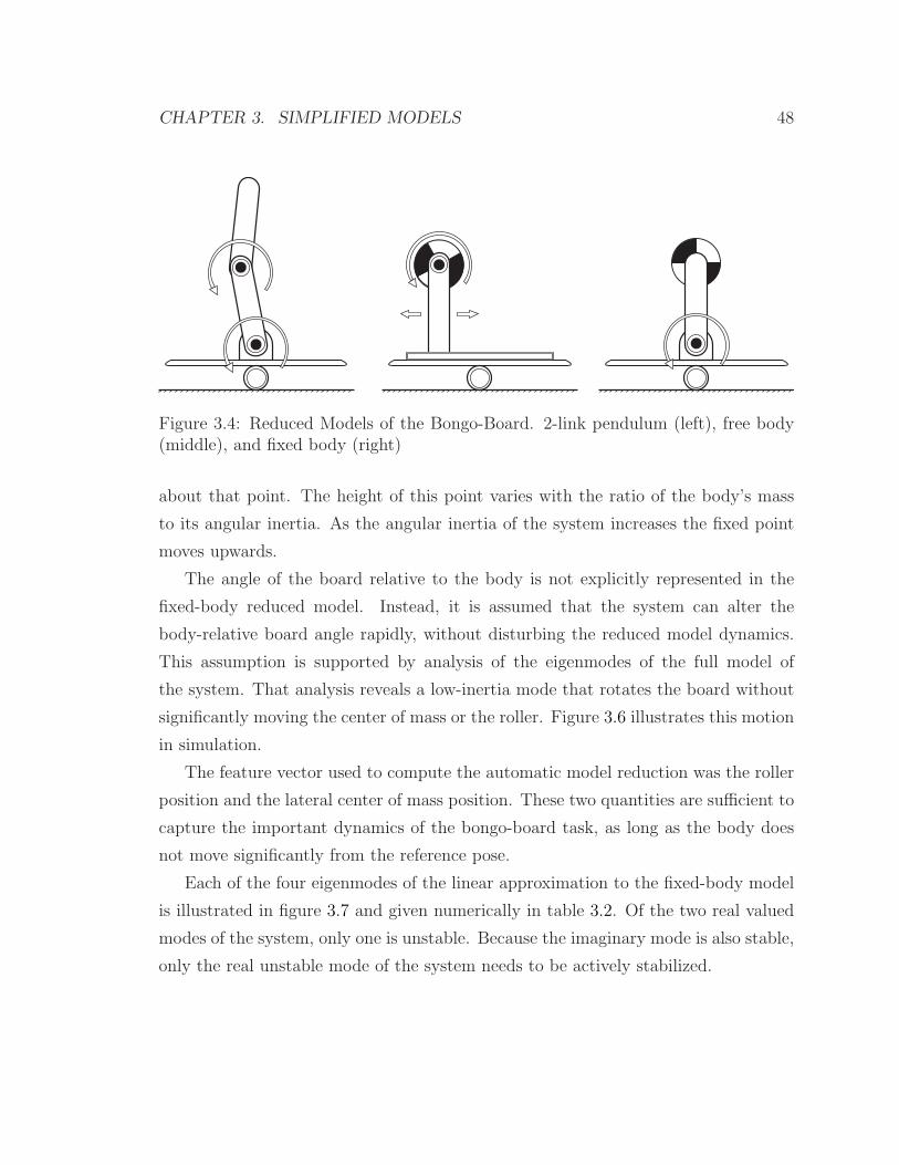
CHAPTER 3. SIMPLIFIED MODELS 48
Figure 3.4: Reduced Models of the Bongo-Board. 2-link pendulum (left), free body(middle), and fixed body (right)
about that point. The height of this point varies with the ratio of the body’s mass
to its angular inertia. As the angular inertia of the system increases the fixed point
moves upwards.
The angle of the board relative to the body is not explicitly represented in the
fixed-body reduced model. Instead, it is assumed that the system can alter the
body-relative board angle rapidly, without disturbing the reduced model dynamics.
This assumption is supported by analysis of the eigenmodes of the full model of
the system. That analysis reveals a low-inertia mode that rotates the board without
significantly moving the center of mass or the roller. Figure 3.6 illustrates this motion
in simulation.
The feature vector used to compute the automatic model reduction was the roller
position and the lateral center of mass position. These two quantities are sufficient to
capture the important dynamics of the bongo-board task, as long as the body does
not move significantly from the reference pose.
Each of the four eigenmodes of the linear approximation to the fixed-body model
is illustrated in figure 3.7 and given numerically in table 3.2. Of the two real valued
modes of the system, only one is unstable. Because the imaginary mode is also stable,
only the real unstable mode of the system needs to be actively stabilized.

CHAPTER 3. SIMPLIFIED MODELS 49
Figure 3.5: For any displacement vector with nonzero board rotation, a single pointin the body’s inertial frame is stationary as the bongo-board moves
3.7.1 Action Space Selection
We experimented with several options for the action space that reflected different
combinations of motions selected from the eigenmodes of the system. We found that
system performance depended almost entirely on the inclusion of motions along the
state vector used to generate the posture displacement illustrated in figure 3.6 and,
in the final controller, chose to include only this action for most trials.
The eigenvectors were computed from the constraint Jacobian Jc and the mass
Table 3.2: Bongo-board Eigenvectors
Unstable Real Mode Oscillating Mode Stable Real ModeEigenvalue 1.38 0.90 ± 0.22i 0.72Roller Position -0.08 -0.01 ± 0.22i 0.09Roller Relative CoM Position 0.28 0 ± 0.10 -0.27Roller Velocity -0.27 0.87 -0.28Roller Relative CoM Velocity 0.91 -0.40 ± 0.02 0.91
CHAPTER 3. SIMPLIFIED MODELS 50
matrixM at the reference pose. Ignoring right hand side forces, we write the equations
of motion:[
M JT
c
Jc 0
][
q
λ
]
= −τ
The left hand side inverse dynamics matrix is inverted using singular value decom-
position to find the forward dynamics matrix. The basis vectors for the action space
are selected from the eigenvectors of that forward dynamics matrix.
We used the eigenvectors of the linearized dynamics at the reference pose as the
action space basis for two reasons. First, because the joint torques required to pro-
duce an acceleration along each eigenmode are orthogonal, the torque magnitude
required to produce an acceleration that is a linear combination of two eigenmodes
grows more slowly than the magnitude of the torque components required to produce
each acceleration component. Figure 3.8 illustrates this effect. Second, because the
resulting accelerations are also orthogonal the total acceleration magnitude is well
behaved in the same manner as the torques. Choosing an action basis in which either
the torques or the accelerations are non-orthogonal can result in either large joint
accelerations or large torques in the full model. This allows a diagonal action cost
matrix to approximate the full model joint torque cost in terms of reduced model
actions, because there are no linear interactions between the reduced model actions
when expanded to the full model space.

CHAPTER
3.
SIM
PLIFIE
DMODELS
51
Figure 3.6: Poses from the system eigenmode corresponding to board rotation without significant mass displace-ment. Note that the vector drawn normal to the board surface moves first to the left and then to the right of thehip center as the board rotates under the robot.

CHAPTER 3. SIMPLIFIED MODELS 52
Figure 3.7: The four eigenvectors of the uncontrolled fixed-body bongo-board model.The leftmost figure is the stable real eigenvector, corresponding to a motion thatresults in the system at rest. The middle figure illustrates is the unstable real eigen-vector, which quickly leads to failure. The final figure illustrates the pair of complexeigenvectors, which correspond to a damped oscillation ending at the rest pose.
F1
F2
F3
O
Figure 3.8: If the torque vectors required to produce two base accelerations are notorthogonal, a situation analogous to that illustrated above can occur. Here, F1 and F2
are the two non-orthogonal torque vectors that produce unit accelerations along theselected action bases. Selecting a desired acceleration along only the first action basisresults in a large increase in the resulting torque magnitude if the second componentmust remain at zero.
Chapter 4
Controller Architecture
Introduction
Dividing a difficult control problem into sub-problems that can be solved indepen-
dently is a common strategy when designing controllers for humanoid robots. This
strategy is effective when the sum of the computational costs of the sub-problems
is significantly less than that of the original problem, and the problem can be de-
composed into sub-problems that are not strongly coupled. The first section of this
chapter introduces a classification of control architectures that use this strategy. The
remainder of the chapter describes the design and implementation of our policy mix-
ing and informed priority control architectures. The specific implementations of the
controller were designed to perform the seesaw balance and bongo-board tasks.
Architectures for software systems are described in terms of components, con-
nectors, and data [Fielding, 2000]. Control architectures, however, represent more
abstract mathematical relationships between functions mapping states to actions.
While the choice of control architecture and software architecture are coupled, the
choice of one does not fully determine the other. Consider, for example, the null-space
control design. As illustrated in figure 4.1, sub-policies can be combined into chains
running from high-level to low-level policies or from low-level to high-level policies,
or their outputs can all be fed into a single mixing function. Each of these possi-
ble software architectures implements the same control architecture in that for the
53

CHAPTER 4. CONTROLLER ARCHITECTURE 54
Balance Policy
Body Posture Policy
End E!ector Policy
Robot
Balance Policy
Body Posture Policy
End E!ector Policy
Robot
Balance Policy
Body Posture Policy
End E!ector Policy
Robot Mixing Function
(a) (b) (c)
Figure 4.1: Three possible software architectures that could be used to implementa hypothetical null-space controller. Diagram (a) shows a controller in which sub-policies receive a control signal from lower priority policies and must augment thissignal with their own output. Diagram (b) shows a controller where sub-policiesreceive the desired output of higher priority policies, and must constrain their ownaction so as not to alter this output. Diagram (c) show a controller where the outputof each sub-policy is combined according to the null-space priority rules by a mixingfunction.
same sub-controllers, the resulting aggregate controller behaves identically. While
it is often tempting to classify control architectures in terms of the structure of the
software architectures typically used to implement them, this tendency obscures im-
portant features of the control architecture by focusing on the features of the software
architecture.
We classify control architectures based on the structure and type of dependencies
between sub-policies. The structure of dependencies between sub-policies is limited
to a small set of possible relationships. A pair of sub-policies may be entirely inde-
pendent of each other, meaning that a change to one policy will not alter the run-time
behavior of the other. Alternately, they may have a directional dependence. When a
directional dependence exists altering the independent policy will alter the behavior
of the dependent policy, but not vice-versa. Logically a final class of sub-policies
with bidirectional dependence exists, but it is unclear in what sense two sub-policies

CHAPTER 4. CONTROLLER ARCHITECTURE 55
Table 4.1: Instances of categories of sub-policy relationships
Controller Control signal System modelVirtual model Independent Full dependency
Trajectory tracking ZMP Directional Dependency Full dependencyPriority null space Directional dependency IndependentInformed priority Directional dependency Directional dependencyPolicy mixing Independent Full dependencyModal control Independent Independent
are distinct if their outputs are co-dependent. We choose to identify groups of co-
dependent policies as a single sub-policy.
In addition to the structure of dependencies within a control architecture, the
type of information transfer that creates those dependencies is also useful for classi-
fication. The two types of information we consider are control signals and models.
These types are elements of the more general categories of run-time data and system
configuration data. To summarize, we classify control architectures based on whether
sub-policies are independent or have one-way dependency relationships, and whether
those dependencies are based on models of sub-policy behavior that can be generated
prior to execution, or on control signals that are generated during execution. Table
4.1 clarifies these possibilities with specific instances of each type of structure.
Control architectures with control signal (or runtime) independence combine the
independently generated outputs from several policies to produce a single combined
output, and can be written, in general as P (x) = M(p1(x), p2(x), . . . , pi(x)), where p1
through pi are the individual sub-policies and M is a mixing function that combines
their individual outputs into a single action. Typically, the output of each sub-policy
has lower dimensionality than P (x), while the sum of the sub-policy output dimen-
sions exceeds the dimensionality of P (x). These methods can be further classified by
the mixing function used to combine the sub-policy outputs. The simplest mixing
functions are superposition methods that combine policies by taking the sum of their
outputs. This method is effective when the policies are designed to be compatible
in this fashion [Stephens and Atkeson, 2010], but is not well suiting to tasks with

CHAPTER 4. CONTROLLER ARCHITECTURE 56
multiple competing objectives. Hierarchical methods based on null space projection
or inequality constraints can resolve conflicts between policies when a clear priority
ordering exists [Saab et al., 2011]. Mixing methods can be used to combine policies
when priority orderings are not clear or vary continuously [Anderson and Hodgins,
2010]. Finally, switching methods that select from one of several possible control sig-
nals, such as state machines, are often used when the system passes through distinct
phases in which different policies are appropriate [Raibert, 1986].
In contrast to methods with control signal independence, a second class of meth-
ods, which we call cascade methods, use the control output of one policy as the control
input to another. Although any directed acyclic graph of dependency relationships is
possible, we are aware only of instances where the dependency relationships form a
single chain. This single-chain control architecture can be expressed as P (x) = u1(x)
where un(x) = pj(x, uj+1(x))∀j < i and ui(x) = pi(x). Here, we refer to u1(x) as
the lowest level sub-policy, and un(x) as the highest level control policy. Perhaps
the most familiar instances of this structure are trajectory tracking implementations
where a high level controller or design process produces a system trajectory, and a
low level controller follows that trajectory [Park and Youm, 2007] [Westervelt et al.,
2003].
The control signal independence of hierarchical methods requires further elabora-
tion. Depending on how sub-policies are defined, it is possible to imagine equivalent
systems in which the control signals have directional dependence, or are independent.
If the sub-policies themselves compute the action space available to policies with
lower priority, then a directional dependence exists in the control signal. However, an
equivalent formulation is to use a mixing function supplied with the desired action of
each sub-policy to compute the output torques. In this case, the control architecture
includes an unlimited number of independent sub-policies and a single mixing func-
tion that combines the output of the sub-policies. If the mixing function is viewed as
an additional sub-policy then these architectures are a sub-set of the set of cascade
architectures. We choose to view hierarchical methods as belonging to the class of
control architectures with control signal independence because this class is the more
limited set.

CHAPTER 4. CONTROLLER ARCHITECTURE 57
The dependence of sub-policy behavior on the offline configuration of other sub-
policies is a less common method for distinguishing control architectures. Very few
situations exist where significant changes in the behavior of one sub-policy require
no modification to any other policy, but typically these modifications are manual
adjustments made by the control engineer. One common example of this type of
manual intervention occurs when the feedback gains used by a trajectory tracking
controller are altered. When this alteration happens the objective function used to
design the trajectories fed to that tracker may need to be updated to reflect the new
capabilities of the tracker. The costs of the trajectory’s acceleration and curvature
keep the system within the envelope where the trajectory tracker can accurately follow
the trajectory. For the trajectory optimizer, the cost function serves as an implicit
model, informing it about the expected behavior of the trajectory tracker. If the
tracker changes significantly, the parameters associated with its implicit model may
need to be manually updated to reflect the change.
In most systems these dependencies are understood by the designer but not ex-
plicitly represented in the control architecture. Informed priority control (Section 4.5,
[Anderson and Hodgins, 2011]) is an example of a control architecture that explicitly
represents these dependencies. This explicit representation allows the output of sub-
policies to change automatically when the offline configurations of the sub-policies
they depend on are changed.
We believe that including directional dependence on offline configuration changes
in the control architecture is important. Without a way to capture these relation-
ships automatically, designers must either manually maintain the dependencies be-
tween sub-policies, typically a time consuming and error prone process, or find ways
to reduce the interdependence of the sub-policies. The belief that reducing the in-
terdependence between sub-policies is desirable has been implicit in much existing
research in humanoid control architectures. For example, null space, zero-dynamics,
modal control, and functional Routhian reductions attempt to make the dynamic
system controlled by a sub-policy independent from the rest of the system.
By designing each sub-policy such that it operates in a space orthogonal to the
other sub-policies in the system, interaction between the sub-policies, and thus the
CHAPTER 4. CONTROLLER ARCHITECTURE 58
need to share information between them, can be minimized. For example, a controller
can be built from a sub-policy concerned only with the motion of the center of mass,
combined with a second sub-policy limited to affecting the system state in the null
space of center of mass motion [Sentis, 2007]. However, because the change in the null
space depends on the combined actions of both sub-policies, neither controller is able
to accurately predict the future state of the full system. Additionally, approaches
that introduce a strong decoupling of the system often require canceling the natural
dynamics of the system, increasing sensitivity to model error. If this decoupling
can be strongly enforced, the configuration dependence between sub-policies can be
reduced or eliminated. While, for fully actuated systems, it is numerically possible to
decouple the system’s dynamics in this way, the energy cost and increased sensitivity
to modeling error can lead to poor performance.
4.1 Related Research in Humanoid Robot Control
Research with robotic humanoids has focused primarily on locomotion, most often
walking gaits on smooth level surfaces, and has relied heavily on task-specific models.
A popular approach to developing a walking controller for a humanoid is to find a
gait trajectory that satisfies a set of constraints such as actuator torque limits and
the need to maintain balance. That trajectory can then be tracked using a controller
designed to maintain stability in the presence of small perturbations and modeling
errors. Variations on this method, using the Zero Moment Point (ZMP) balance con-
straint, are used by most humanoid robots with electric motors, including the HRP,
ASIMO, HUBO, KHR, HSR, and the WABIAN series. Exceptions include the elec-
tric biped developed by CMU and ATR [Morimoto et al., 2003] and Delft’s biped
Meta [Schuitema et al., 2005]. Open questions in this area include the design of refer-
ence trajectories that increase the natural appearance, efficiency, or robustness of the
resulting gait, and the development of new trajectory tracking controllers that enable
recovery from larger perturbations than the local balance controller can stabilize.
The primary challenge to stable control of humanoid robots during gait is loss
of balance. Existing approaches to maintaining stability can be categorized by their

CHAPTER 4. CONTROLLER ARCHITECTURE 59
definition of balance. Quasi-static balance constraints require that the robot only
enter states that are stable in a static analysis. Given a planar support surface this
constraint implies that the robot’s center of mass (CoM) lies above the convex hull of
the points of contact between the robot and the support surface. If this constraint is
obeyed, and the robot moves sufficiently slowly, it cannot fall unless pushed. A more
common class of balance constraints requires that the robot only perform actions that
allow its feet to remain in flat contact with the ground [Vukobratovic, 1973]. The ZMP
constraint is the most commonly used member of this class. It is limited to the case of
a robot with flat feet moving on a locally flat surface. The final and most general class
of balance definitions are those that have no definition as instantaneous constraints.
These methods include the multi-step Poincare stability analysis of passive dynamic
walking systems, point foot walkers, humans, and robots with control policies that do
not produce gaits that obey instantaneous constraints [Garcia et al., 1998, Goswami
et al., 1996].
The ZMP is the point on the ground plane at which the net moment of the forces
acting on the robot have no horizontal component. When the ZMP falls within the
region of support it is equivalent to the center of pressure (CoP). If the ZMP is
maintained within the region of support then the feet will not rotate about a non-
vertical axis. A more intuitive understanding of the ZMP constraint is provided by
the idea that as long as the robot’s motions do not violate the constraint, the feet can
be treated as if they are rigidly attached to the ground. Because natural human gait
involves rolling contact with the ground, some researchers believe that this constraint
precludes natural walking motion. The utility of the ZMP model derives from its
ability to reduce the problem of balance to the problem of controlling the change in
total system momentum. This decoupling allows the control problem to be factored
into two decoupled stages, first determining the center of mass trajectory and then
the joint trajectory that produces the current desired center of mass acceleration.
Another tradition in controlling legged robots was pioneered for running hop-
pers [Raibert, 1986] and later extended to other gait styles [Hodgins and Raibert,
1991, Hodgins, 1991]. These controllers are based on an engineered model, the single
link inverted pendulum (SLIP) [Blickhan and Full, 1993] that describes the exchange
CHAPTER 4. CONTROLLER ARCHITECTURE 60
between potential and kinetic energy observed in many animal gaits using a pogo-
stick-like model. A further simplification of that model is used to design the hopping
controller. This simplification assumes that weakly coupled modes of the full non-
linear dynamics are in fact fully decoupled and linear. In particular, the forward
velocity of the center of mass, the angular momentum, and the vertical velocity of
the center of mass are all considered to be decoupled and are controlled by indepen-
dent linear controllers. An important feature of this model is that the action spaces
of each independent controller is completely decoupled from the other controllers by
its implementation.
Both constraint-based trajectory optimization approaches, like ZMP walking, and
approaches based on finite state machines and linear controllers, like the Raibert
hoppers, use the sub-policy strategy as a key component of their approaches. The
ZMP approach separates balancing from the remainder of gait by ensuring that any
motion used to achieve gait satisfies the ZMP constraint. This assumption permits
a controller with a decoupled, tiered architecture, where the lowest level computes
joint commands that stabilize the robot as it tracks a trajectory computed by a
higher level. The controllers for the Raibert hoppers decouple the problem of biped
hopping into the problems of maintaining body pitch, maintaining forward velocity,
and maintaining hopping height.
4.2 Trajectory Optimization
Trajectory optimization techniques are a component of many of the sub-policies we
consider. These methods can be used to transform an unstable, inefficient trajectory
that violates physical constraints into a physically plausible, balanced, and efficient
trajectory, if the initial guess is sufficiently close to a viable solution. While trajectory
optimization is already used to design trajectories for humanoid robots, the methods
developed by the graphics community are of particular interest because they are
explicitly designed to make use of motion capture data both for the initial guess
of an optimal trajectory and to constrain the search space that the optimizer must
explore. Additionally, because animators desire characters that can perform a range of

CHAPTER 4. CONTROLLER ARCHITECTURE 61
actions in varied environments, trajectory optimizers developed for human animation
tend to be designed to operate on a more general set of inputs than domain specific
optimizers developed for periodic tasks such as gait. These features suggest that
the trajectory optimization techniques developed for creating physically plausible
animations of human figures may also be well suited for creating viable reference
trajectories for humanoid robots.
Trajectory optimization techniques are used by both graphics researchers and
roboticists to create motions for both animated and robotic humanoid figures. Tra-
jectory optimization refers to a class of methods for determining solutions to a system
of differential equations that minimize a functional of the solution while satisfying a
set of constraints. A taxonomy of these methods based on salient features in their
design is useful in a discussion of their application to robotics and animation. One
such feature is whether a method minimizes the objective function directly by mod-
ifying the dependent variables subject to the constraints, or indirectly by using the
calculus of variations to find a solution to the ODEs that satisfy a necessary condition
for optimality, such as the Hamiltonian described by Pontryagin’s Minimum Princi-
pal [Stengel, 1994]. Because indirect methods are often numerically unstable and
require a more accurate initial guess [Schwartz, 1996], we consider only a selection of
direct methods in this work.
Direct methods alter some or all of the independent variables to minimize the
objective function. While they produce solutions that are strictly integrable, com-
puting derivatives of the objective and constraint functions can become numerically
unstable because the effects of actions taken earlier in time can grow exponentially
over time. Shooting methods are a popular class of direct methods. These methods
integrate the equations of motion forward or backward in time from a known state,
varying the control input to achieve an optimal trajectory. Computing the gradient of
the objective function is challenging because the influence of control inputs at earlier
times can be amplified by the integration, resulting in poor numerical conditioning
in the resulting Jacobian. Multiple shooting methods can ameliorate this problem by
dividing time into a series of epochs that are integrated separately [Morrison et al.,
1962].

CHAPTER 4. CONTROLLER ARCHITECTURE 62
Differential dynamic programming is another method that integrates forward in
time [Jacobson and Mayne, 1970]. This method iteratively improves a trajectory us-
ing quadratic approximations of the value function computed using linear models of
the system at many points along the trajectory. It has the advantage of producing not
only the optimal control inputs, but also an optimal linear policy at each discretization
point. Researchers have suggested that improvements to the value function approx-
imation could be made by fitting a quadratic model to values obtained by forward
simulation of the system dynamics [Tassa et al., 2007].
A separate class of direct trajectory optimization methods, referred to as direct
collocation methods, vary both the sequence of states and the control inputs. The
equations describing the system dynamics are treated as additional constraints. All
constraints are enforced only at discretization points, meaning that the system cannot
necessarily be integrated forward in time. Direct collocation methods are popular
because they are numerically stable and tend to converge from less accurate initial
guesses than other methods [Schwartz, 1996]. In the graphics community, trajectory
optimization methods were introduced by Witkin and Kass [1988] under the name
spacetime constraints. The optimization approach presented in that work and used
often in the graphics literature is a direct collocation method [von Stryk and Bulirsch,
1992].
Trajectory optimization for high dimensional systems can be computationally in-
tensive due to the need to compute the Jacobian of cost and constraint parameters
with respect to the free parameters. In the traditional formulation of the problem,
joint torques appear in the objective function and require O(n2) time to compute,
where n is the number of degrees of freedom in the system. Fang and Pollard [2003]
demonstrated a method for computing the force and torque about a single joint or
the kinematic root in O(n) time. They showed that if the objective function is refor-
mulated in terms of joint accelerations rather than torques, and physical constraints
are specified in terms of wrenches applied to the kinematic root, then a significant
speedup to trajectory optimization for systems with many degrees of freedom can be
achieved.

CHAPTER 4. CONTROLLER ARCHITECTURE 63
4.3 Policy Mixing Control Framework
This section describes the policy mixing control framework [Anderson and Hodgins,
2010] we developed for the seesaw task. The Informed Priority framework we describe
in section 4.5 is a later development that supersedes the design described in this
section. Understanding the design of Policy Mixing Control helps to motivate the
development of Informed Priority control.
The policy mixing control framework composes fully independent sub-policies and
does not require an explicit ordering of control priorities. It computes desired joint
torques by assigning a numerical weight to each of several sub-policies and finding
joint torques that best reproduce the desired outputs of these sub-policies. Given the
desired actions from each component policy, the controller computes joint torques that
minimize the sum of the weighted deviations from the desired action of each policy.
For example, our balance policy provides desired contact forces, while the posture
policy provides desired joint accelerations. While it is not, in general, possible to
choose a set of joint torques that simultaneously produces the desired contact forces
and joint accelerations, we can choose the set of joint torques that minimizes the
total weighted difference between the actual and desired contacts forces and joint
accelerations.
We developed the policy mixing control framework because we believed that the
strict priority ordering present in hierarchical control architectures resulted in insta-
bility due to impedance mismatches. As a single example of this problem, consider a
two link planar arm. Suppose a two-level hierarchical controller is used, with a high
level control policy that controls the distance between the end effector and the origin,
and a low level control policy that tries to return the system to a rest pose. The end
effector impedance is a combination of the impedance of the high level policy with the
impedance of the low level policy in the null space of the high level level policy’s state
space. If the impedances of these two policies are significantly different, chattering
can occur. By softening the hierarchical constraints from a subspace projection to a
least squares combination of the inputs we hoped to reduce this problem.

CHAPTER 4. CONTROLLER ARCHITECTURE 64
4.3.1 Dynamics
Our controller combines several component policies with different dimensionality and
weight to produce by a full set of desired joint torques. Combining these policies
requires a dynamic model of the system, and a mathematical description of how joint
torques relate to the output values produced by the component policies. Given this
information, we can solve a system of linear equations to produce the output joint
torques. Unlike other formulations of full body inverse dynamics [Mistry et al., 2010,
Nakanishi et al., 2007], the solution vector for this linear system includes all acceler-
ations, contact forces, and joint torques, avoiding the need to explicitly compute the
inverse of the mass matrix, at the expense of solving a larger system of equations.
We write this solution vector x =[
q λ τ]T
.
4.3.2 Policy Mixing
All the sub-policies we combine produce both a desired action vector, Udes, and an
action error matrix, Jact. We compute Jact =∂Udes
∂xsuch that
Uerr = Jactx− Udes
Here, Uerr goes to zero when the computed torque solution vector exactly reproduces
the desired policy action. For example, Udes could express a desired lateral accelera-
tion for the system’s center of mass. In this case, Uerr would be the difference between
this desired acceleration and the true acceleration of the system’s center of mass. The
non-zero terms of Jact would be the Jacobian of the center of mass acceleration with
respect to the joint accelerations in the solution vector.
Given N policies and a set of corresponding component policy outputs Uerr, and
policy weights w, the total output error is
E =N∑
i=1
wiUerri =
w1Jact1...
wNJactN
x−
w1Udes1
...
wNUdesN
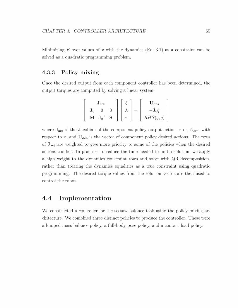
CHAPTER 4. CONTROLLER ARCHITECTURE 65
Minimizing E over values of x with the dynamics (Eq. 3.1) as a constraint can be
solved as a quadratic programming problem.
4.3.3 Policy mixing
Once the desired output from each component controller has been determined, the
output torques are computed by solving a linear system:
Jact
Jc 0 0
M JcT S
q
λ
τ
=
Udes
−Jcq
RHS(q, q)
where Jact is the Jacobian of the component policy output action error, Uerr, with
respect to x, and Udes is the vector of component policy desired actions. The rows
of Jact are weighted to give more priority to some of the policies when the desired
actions conflict. In practice, to reduce the time needed to find a solution, we apply
a high weight to the dynamics constraint rows and solve with QR decomposition,
rather than treating the dynamics equalities as a true constraint using quadratic
programming. The desired torque values from the solution vector are then used to
control the robot.
4.4 Implementation
We constructed a controller for the seesaw balance task using the policy mixing ar-
chitecture. We combined three distinct policies to produce the controller. These were
a lumped mass balance policy, a full-body pose policy, and a contact load policy.

CHAPTER 4. CONTROLLER ARCHITECTURE 66
4.4.1 Lumped mass policy
The lumped mass policy used a simplified model of the robot. The robot’s body was
treated as a single rigid mass (figure 4.2). The lumped mass model reduction is
yp =
r
θ
p
L
=
CM(q)
O(q)
p(q, q)
L(q, q)
= Rp(q, q)
where r is the lumped mass position, θ is the lumped mass Euler angle orientation, p
is the lumped mass linear momentum, and L is the lumped mass angular momentum.
The function CM(q) computes the center of mass of the robot using the rigid body
model,O(q) computes the orientation of a “key body” on the robot (we used the upper
torso), p(q, q) computes the linear momentum of the robot, and L(q, q) computes the
angular momentum of the robot.
The lumped mass policies take the state of the lumped mass and use a linear
policy to produce a desired total center of mass load, or a desired center of pressure
location. We selected a center of pressure output for the seesaw task, but also used the
total CoM load output successfully for standing balance. The output is constrained
so that the center of pressure corresponding to the desired total load remains within
the region of support. When the lumped mass policy produces contact loads directly,
the relationship between x and Up is defined in terms of the λ component of x:
Uerr = Up −
[
fl + fr
τl + τr + (rCM − rl)× fl + (rCM − rr)× fr
]
When the lumped mass policy is producing a desired center of pressure the action
error is
Uerr =[
τl + τr + (rCoP − rl)× fl + (rCoP − rr)× fr
]
Where τl and τr are the moments about the left and right feet, fl and fr are the
forces on the left and right feet, rCoP is the location of the center of pressure, and rr
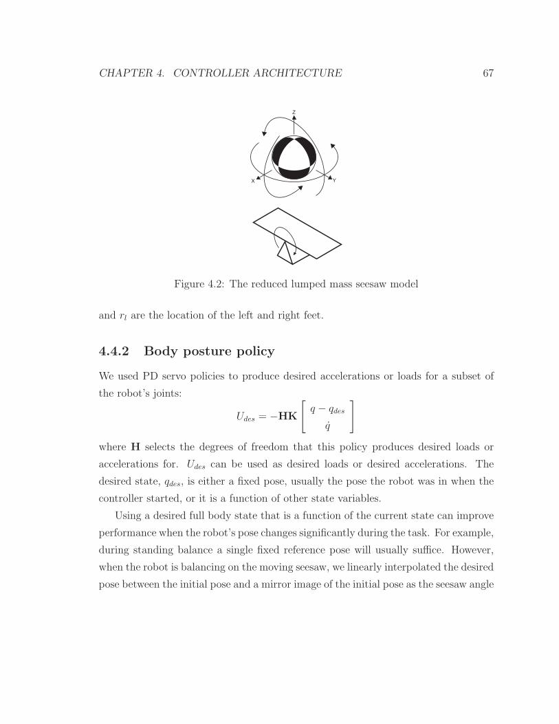
CHAPTER 4. CONTROLLER ARCHITECTURE 67
YX
Z
Figure 4.2: The reduced lumped mass seesaw model
and rl are the location of the left and right feet.
4.4.2 Body posture policy
We used PD servo policies to produce desired accelerations or loads for a subset of
the robot’s joints:
Udes = −HK
[
q − qdes
q
]
where H selects the degrees of freedom that this policy produces desired loads or
accelerations for. Udes can be used as desired loads or desired accelerations. The
desired state, qdes, is either a fixed pose, usually the pose the robot was in when the
controller started, or it is a function of other state variables.
Using a desired full body state that is a function of the current state can improve
performance when the robot’s pose changes significantly during the task. For example,
during standing balance a single fixed reference pose will usually suffice. However,
when the robot is balancing on the moving seesaw, we linearly interpolated the desired
pose between the initial pose and a mirror image of the initial pose as the seesaw angle

CHAPTER 4. CONTROLLER ARCHITECTURE 68
changed from its initial angle to the inverse of the initial angle.
qdes = αqinit + (1− α)mirrorx(qinit)
α =θcur − θinit2 |θinit|
Here, θ is the angle of the board. This computation provides desired poses with a
center of mass near the desired center of mass as the board moves. This computation
is a simpler and faster operation than solving the inverse kinematics to determine a
desired full body pose that matches the desired center of mass location and preserves
the foot contact constraint.
The relationship between Udes and x depends on whether desired torques or ac-
celerations are produced, but is simple in either case:
Uerr = Udes − Sτ
Uerr = Udes − Sq
4.4.3 Static contact load policies
The lumped mass balance policies produce a desired total ground contact load, but
provide no information about how this load is to be divided between the feet. Because
no higher weight policy fully determines the contact forces, the PD servo policies can
produce undesirable contact loads, even when they have very low weights.
To solve this problem, a third type of policy, the static contact load policy, is
introduced. This policy’s output is constant in the robot’s state, and always requests
that the foot contact torques on each foot be equal to a constant value, or that the
difference between the torques on each foot be constant. The relationship between
the components of the solution vector x and Udes is
Uerr = G(τl − τr)
Uerr =
[
Gτl
Gτr
]
CHAPTER 4. CONTROLLER ARCHITECTURE 69
where G selects the particular axis being controlled by the static contact load policy.
In our experiments on the seesaw, the static contact load policy tried to maintain
zero torque about the foot load cells along the X axis.
4.4.4 Solving for Desired Torques
We solve the system by applying a high weight to the dynamics constraint rows and
solving with QR decomposition. The desired torque values from the solution vector
are then used to control the robot.
The contact constraint Jacobian is computed numerically using a finite difference
method. Each column of Jc is computed by altering the corresponding component of
the current pose and computing the resulting change in the translation and rotation
of each foot relative to the seesaw. The time derivative of this Jacobian, Jcq, is
computed by Euler-integrating the current pose forward in time by a 1e− 8 second,
computing a new contact Jacobian at this new pose, and taking the difference between
the current and future contact Jacobians.
4.5 Informed Priority Control
Informed priority control is a serial cascade control design that introduces explicit
dependencies between policies for both run time and configuration time information.
It is a complete replacement for the policy mixing design described in the previous
section. Like all cascade controllers, control signal information travels down the
cascade, with the control signal output of one policy used as the control input to the
next. In our case, this cascade produced a final torque vector that is sent to the robot
hardware. In addition to this downward information flow, models of each controller
travel up the cascade in the form of automatically generated models of the behavior of
the partial downstream cascade. These models are used by the sub-policies to predict
the future behavior of policies lower in the cascade, allowing every policy to have a
complete and coherent model of the system it controls. This section describes the
informed priority control framework and demonstrates a particular implementation
CHAPTER 4. CONTROLLER ARCHITECTURE 70
of that framework for control of a humanoid robot balancing on a bongo-board.
Informed Priority Control differs from existing cascading control or inner and outer
loop control designs in that it includes a general facility for automatically building
reduced models of each inner loop system. This facility provides outer loop controllers
are provided with linear models of the system they control, linearized about arbitrary
points in the full system’s state space.
Based on the difficulties we encountered applying policy mixing control, we de-
veloped a new control design that resolves some of these problems. In the policy
mixing formulation, none of the component policies has information about any other
policy. Informed priority control informs component policies about the behavior of
other policies in two ways. First, high-priority policies use models of the system that
include the behavior of low priority policies. Second, low priority policies take the
output of the high priority policies as their control inputs.
Informed priority control combines sub-policies by passing the control output of
one policy to the control input of another, eventually connecting all sub-policies into
a single cascade. Additionally, every policy is provided with a model of the system its
control output is passed to. We automatically construct these models of the behavior
of the existing cascade before adding each additional link.
For example, the lowest-level policy in the cascade receives only the rigid body
model of the robot, while the second to lowest policy receives a model of the closed
loop system that includes both the first policy and the rigid body model. Figure 4.4
shows which parts of the control system are included in the model presented to each
policy. While the informed priority control framework is defined without reference to
model reduction, the automated model construction process it uses can build models
in a reduced feature space, if this reduction is desired.
Each model fully describes the behavior of the system controlled by the policy
using that model. Actions taken by policies higher in the cascade are not predicted
by the model. However, the accuracy of the model is unaffected because the output
of those higher-level policies is presented as a control input to the policy using the
model. Direct analysis of the stability and optimality of controllers built using the
informed priority control framework is possible because model error is bounded and
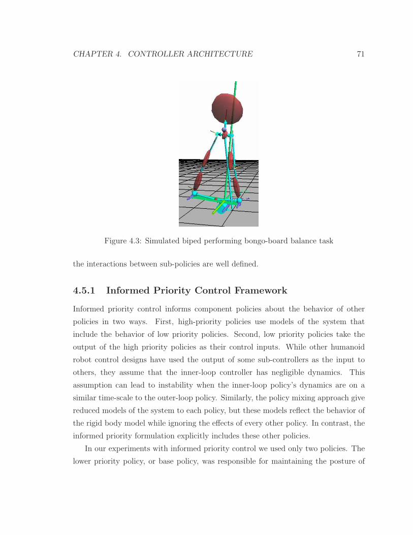
CHAPTER 4. CONTROLLER ARCHITECTURE 71
Figure 4.3: Simulated biped performing bongo-board balance task
the interactions between sub-policies are well defined.
4.5.1 Informed Priority Control Framework
Informed priority control informs component policies about the behavior of other
policies in two ways. First, high-priority policies use models of the system that
include the behavior of low priority policies. Second, low priority policies take the
output of the high priority policies as their control inputs. While other humanoid
robot control designs have used the output of some sub-controllers as the input to
others, they assume that the inner-loop controller has negligible dynamics. This
assumption can lead to instability when the inner-loop policy’s dynamics are on a
similar time-scale to the outer-loop policy. Similarly, the policy mixing approach give
reduced models of the system to each policy, but these models reflect the behavior of
the rigid body model while ignoring the effects of every other policy. In contrast, the
informed priority formulation explicitly includes these other policies.
In our experiments with informed priority control we used only two policies. The
lower priority policy, or base policy, was responsible for maintaining the posture of

CHAPTER 4. CONTROLLER ARCHITECTURE 72
Plant
Policy 1
Policy 2
Policy 3
Plant
Policy 1 Policy 2 Policy 3
Policy Mixer
Figure 4.4: Policy Mixing and Informed Priority Control Diagrams. Policy mixingcontrol (left) produces a single output from many policies that use the same systemmodel. Informed priority control (right) presents each policy with a model thatincludes the behavior of all lower priority policies.
the robot. It produced desired joint torques based on the current state of the robot
and a desired state set by the higher priority policy. The base policy was designed to
work well over a wide range of tasks, and to track the desired pose without oscillation.
The informed priority control framework provides predictive models of the policies
lower in the control cascade to those higher in the chain. This arrangement allows
higher level policies to design their control inputs in order to accommodate the future
behaviors of lower level policies. For example, a disturbance to the upper torso
may trigger a response from a low-level posture controller. This response will alter
the future center of pressure, and may require that the balance controller alter its
planned future actions to compensate for the upper body correction. Without this
model, the balance controller would have no prior expectation of the upper body
correction. Additionally, if the low-level policy’s gains are re-tuned, the higher level
policy’s model is automatically updated to reflect the new response rate of the low
level controller. This updated model permits the higher level policy to automatically
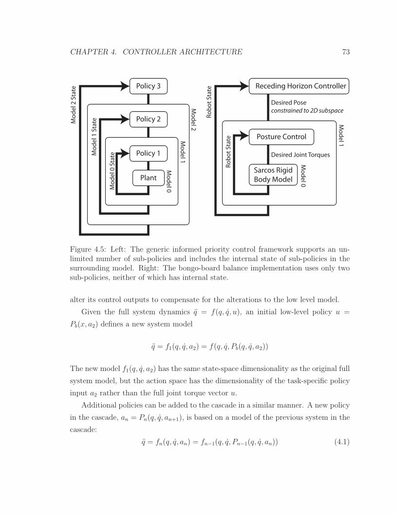
CHAPTER 4. CONTROLLER ARCHITECTURE 73
Plant
Policy 1
Policy 2
Policy 3
Mo
de
l 2
Mo
de
l 1
Mo
de
l 0
Sarcos Rigid
Body Model
Posture Control
Receding Horizon Controller
Mo
de
l 1
Mo
de
l 0
Desired Pose
constrained to 2D subspace
Desired Joint Torques
Ro
bo
t S
tate
Mo
de
l 2 S
tate
Mo
de
l 1 S
tate
Ro
bo
t S
tate
Mo
de
l 0 S
tate
Figure 4.5: Left: The generic informed priority control framework supports an un-limited number of sub-policies and includes the internal state of sub-policies in thesurrounding model. Right: The bongo-board balance implementation uses only twosub-policies, neither of which has internal state.
alter its control outputs to compensate for the alterations to the low level model.
Given the full system dynamics q = f(q, q, u), an initial low-level policy u =
Pb(x, a2) defines a new system model
q = f1(q, q, a2) = f(q, q, Pb(q, q, a2))
The new model f1(q, q, a2) has the same state-space dimensionality as the original full
system model, but the action space has the dimensionality of the task-specific policy
input a2 rather than the full joint torque vector u.
Additional policies can be added to the cascade in a similar manner. A new policy
in the cascade, an = Pn(q, q, an+1), is based on a model of the previous system in the
cascade:
q = fn(q, q, an) = fn−1(q, q, Pn−1(q, q, an)) (4.1)
CHAPTER 4. CONTROLLER ARCHITECTURE 74
The ability of the policy Pn to stabilize the system fn(x, a) depends on the choice
of the underlying policies Pi(x, a) where i ∈ {1 . . . (n − 1)}. In particular, the base
policy should attempt to stabilize as many modes of the full system as possible, avoid
violating constraints, and keep fn(x, a) smooth.
The models of the system constraints and cost functions are also updated and
supplied to each sub-policy as in equation 4.1. If a simplified model is desired at
some point in the chain, it can be built using the normal model reduction procedure.
Note that even if a reduced model is used at one point in the chain, policies further
up the chain are not limited to the state space of this model, and can build their own
models in the full state space.
4.6 Implementation of Informed Priority Control
We used an informed priority controller for the bongo-board balance task. This
controller used a base policy that was responsible for maintaining the overall posture
of the robot and maintaining contact between the robot’s feet and the bongo-board.
The input to the base policy was a desired posture, generated by a second task-
specific policy. We experimented with two distinct designs for this task-specific policy,
a receding horizon trajectory optimization based controller, and a mode-switching
controller. In this section, the base policy and the task-specific policies are described
in detail.
4.6.1 Base Policy
The postures chosen by the task policy must be transformed into desired joint torques
before they can be sent to the individual joint controllers. The base policy performs
this transformation. Moreover, the role of the base policy is to reduce the dimen-
sionality of the action space presented to the task policy without making the system
uncontrollable due to underactuation. Figure 4.6 illustrates the relationship between
the task and base policies. In the final bongo-board simulation controller, the task
controller selected a pose from a one or two dimensional space of poses, and the base

CHAPTER 4. CONTROLLER ARCHITECTURE 75
policy tracked this desired pose quickly and without oscillation.
We defined a base policy that stabilized the joint angles of the robot, but not
the bongo-board state. This policy was the sum of gravity compensation torques
and a linear PD feedback term that provided well damped responses to inputs. The
baseline policy was not designed to stabilize the system on the bongo-board. The
goal of the baseline policy was to track the desired pose control signal generated
by the higher level bongo-board task controller. To achieve this goal, the baseline
controller included the rigid body mode of the bongo-board when calculating both
the damping gains for the linear component of the policy and the variance minimizing
gravity compensation torques. The result of this base policy is that the joint angle
coordinates of the system model presented to the task-specific controller are passively
stable. The only unstable coordinates in the model presented to the task controller
are those that describe the state of the bongo-board. We write the combination of
the linear feedback term and the gravity compensation term as:
Pb(x, a) = −K(x− inflate(u)) +G(x)
Here inflate(u) produces the full state pose corresponding to the task action u. Be-
cause the action space is linear in this case, inflate(a) ≈ Uu where the matrix U
contains the basis poses for the action space. Because the kinematic constraints are
nonlinear in the state space of the full model, this linear inflation will produce desired
poses that violate the kinematic contact constraints. We used a computationally ef-
ficient method of correcting these errors. This method pre-computed poses near the
space spanned by U that do not violate the kinematic constraints, using sequen-
tial quadratic programming. Then, at runtime, it used locally weighted regression
[Atkeson et al., 1997a] to interpolate between these points to construct poses that
significantly reduced kinematic constraint violations. While the system did not re-
quire this correction term in simulation, in hardware the limited friction between the
board and feet allowed the feet to slip when the desired pose moved far from the
reference state, if this term was not present.
The remainder of this section discusses the procedure we used to design K so that

CHAPTER 4. CONTROLLER ARCHITECTURE 76
Robot
Robot Model
Base Policy
Task Policy
State Estimatorestimated state prediction error
joint torques
simple action
Figure 4.6: Control flow diagram for task and base policy
the system would respond quickly to changes in u without being underdamped, and
the construction of G we used to reduce sensitivity to model error and accommodate
unactuated degrees of freedom in the model.
4.7 Linear Feedback Component
The linear feedback policy K was designed with the intent that the robot would track
the desired position specified by the input a quickly, but without oscillation. We tried
three methods for designing K. While all three methods produced stable controllers,
only one design process gave meaningful tuning inputs that allowed us to adjust the
behavior to match the desired performance.
The first design process we used was to linearize the system dynamics, including
the gravity compensation term, about a reference pose and design a linear quadratic
regulator to stabilize the system about this point. However, the gains produced by
the LQR process tended to produce damping gains that resulted in underdamped
oscillation. We were unable to produce the desired performance characteristics by
tuning the Q and R cost matrices directly because the relationship to the whole
body behavior is complex. We found that it was possible to produce sets of gains
that were critically damped but not stiff enough, or stiff gains that were underdamped,
but were unable to find a set of cost matrices that produced the desired body stiffness
while remaining critically damped. It was unclear how to modify the cost function
CHAPTER 4. CONTROLLER ARCHITECTURE 77
to produce the specific behavior changes we wanted, and difficult to manually tune
because there are many parameters.
The second design process we used was to hand tune independent feedback gains
for each joint, in an attempt to reduce the number of parameters that required tuning
and to clarify the relationship between those parameters and the system’s behavior.
This approach worked poorly because the best gains for a specific joint depend on
the configuration of the entire system. For example, the inertia of the leg observed
from the hip flex extend joint is much larger when the knee is straight than when the
knee is fully bent. Additionally, without off diagonal terms in the feedback matrix the
system tends to be underdamped when using the minimum stiffnesses necessary to
overcome model error in the gravity compensation and the maximum damping gains
that do not cause uncontrolled oscillation.
The final design process we used, and the one that produced the desired behavior,
was based on identifying the eigenmodes of the system and treating those modes,
instead of the individual joints, as the basis for independent feedback gains. This
preserved the smaller number of parameters that required tuning while reducing the
effects of not having feedback coupling between modes. We computed a linear ap-
proximation to the forward dynamics of the full model at a reference pose and found
the eigenvectors of this forward dynamics matrix. Because this matrix transforms
generalized control forces into generalized accelerations, the eigenvalues correspond
to the inverse of the effective inertia of each independent mode. Tuning independent
linear controllers in this modal space proved easier than tuning full state Q and R
matrices.
The linear feedback terms are computed using the singular value decomposition of
the forward dynamics, computed from the inverse dynamics D and a selection matrix
s that removes elements that correspond to base coordinates, constraint forces, or

CHAPTER 4. CONTROLLER ARCHITECTURE 78
constraint violations, leaving only those elements that correspond to joints:
D =
[
M Jc
JT
c 0
]
D
[
q
λ
]
=τ
0
q = sD−1sτ = USVTτ
Because each torque vector in the rows of V produces an acceleration that is orthog-
onal to the acceleration produced by any other torque vector in V, we can design the
linear feedback term for each mode without considering potential interactions with
other feedback terms. In practice, we choose a uniform stiffness value that is applied
to every mode and a damping term that is proportional to the square root of the
effective inertia of the mode.
Kp = VkpS+UT
Kd = Vkd(
S+)
1
2 UT
We found that the best performance could be obtained by making further adjustments
to the overall gain scaling for each mode. This adjustment allowed us to increase the
overall stiffness and damping of the system while not increasing the gains of modes
that would have developed instabilities at these higher gains. Specifically, we dropped
the feedback gains for the first five modes by half, and increased the damping gains
for the largest three modes by twenty five percent. When underdamped oscillations
did develop during tuning it was easy to diagnose which mode’s gains needed to be
adjusted because the oscillation typically limited itself to only one mode, as expected.
Figure 4.7 shows an example of this behavior where the gain on mode three has been
increased past the stable limit. If this same data were viewed in terms of joint angles
the oscillation would appear on every plot, making it exceedingly difficult to determine
which gains needed to be adjusted.
Because of the contact constraints that prevent the feet from moving relative to
each other, the six modes with the largest apparent inertia correspond to the null

CHAPTER 4. CONTROLLER ARCHITECTURE 79
space of Jc. If the linear model of the system’s kinematics were perfectly accurate,
the system would be unable to move in this null space. However, because Jc is
slightly inaccurate, and because JC changes as the system state changes, we treat
these six modes as if they were unconstrained modes with a moderate inertia and
supply feedback terms for them by replacing the zeros on the diagonal of S with a
uniform non-zero value.
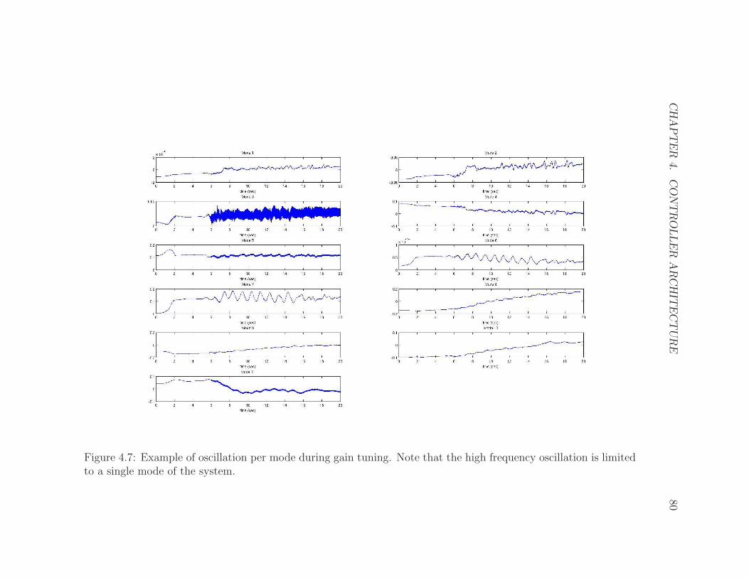
CHAPTER
4.
CONTROLLER
ARCHIT
ECTURE
80
Figure 4.7: Example of oscillation per mode during gain tuning. Note that the high frequency oscillation is limitedto a single mode of the system.
CHAPTER 4. CONTROLLER ARCHITECTURE 81
4.8 Gravity Compensation Component
We compensated for the effect of gravity on the actuated joints. In a fully actuated
system gravity compensation can be achieved by using the inverse of the right hand
side forces as the joint torques. Because the bongo-board joints and the root coor-
dinates are unactuated in our model it was not possible to apply the inverse of the
right hand side forces directly. We chose to compensate only for gravitational accel-
eration at the actuated joints and allow the unactuated degrees of freedom to have
uncontrolled accelerations. Because the loop constraint eliminates several degrees of
freedom, there is not a unique solution for the set of torques that compensate for grav-
itational acceleration at the joints. We resolved this redundancy by minimizing an
objective function defined by the expected variance in the resulting joint accelerations
due to load cell scale factor miscalibration.
When the robot is standing there is typically a redundant degree of freedom in
each leg corresponding to an internal motion of the leg without changing the location
of either the hip or the foot. This degree of freedom usually involves rotating the
knee about the line connecting hip to ankle using joints in the hip and ankle. This
situation is similar to the case of a human with fixed hip and foot positions.
Transmitting a large gravitational load across a free body with low inertia requires
the actuators on both sides of that body to apply counteracting forces. If these forces
are slightly imbalanced a large acceleration of the low mass body will result. Because
the remaining degree of freedom in the leg has a low effective moment of inertia, small
load cell miscalibrations can cause large accelerations in this mode.
Consider figure 4.8 as a simplified example of a gravity compensation problem
with redundancy. Gravity compensation requires that a + b = 10g and c − b = 1g.
This constraint leaves one unconstrained degree of freedom in the solution. The
torque vector that minimizes the sum of squared torques as expressed by the objective
function τTIτ is
τ =
a
b
c
=
7
4
3
g

CHAPTER 4. CONTROLLER ARCHITECTURE 82
10kg
1kgab
c
Figure 4.8: Example of a system in which gravity compensation at the joints is under-determined. The torque minimizing and variance minimizing solutions are distinct.
However, if we assume that each actuator will apply a force with an error that
grows linearly with the applied force, we can define an alternate objective func-
tion that minimizes the acceleration error due to this force error. Using this error-
minimizing objective function the gravity compensation forces are
τ =
a
b
c
=
10.42
−0.42
0.57
g
We construct the objective function for the variance minimizing redundancy resolu-
tion using the forward dynamics. Given a forward dynamics matrix A with columns
An, we use the magnitude of each column vector as the cost for the corresponding
torque. Assuming that the scale factors for the torque feedback sensor on each joint
have independent error with uniform variance σ, the variance of the torque error for
any particular joint is στTAT
nAnτ . Using a uniform cost for acceleration error across
all joints we can compute the acceleration error variance:
E [V ar(q)] = σ∑
i
∑
j
(Ai,jτj)2 = στT
AT
1A1
. . .
AT
nAn
τ

CHAPTER 4. CONTROLLER ARCHITECTURE 83
This matrix can be used as the quadratic cost function in solving a quadratic pro-
gramming problem to find a set of torques that produces zero acceleration at the
actuated joints.
4.9 Enforcing Output Constraints
The desired torques that are computed as the sum of the gravity compensation and lin-
ear feedback components may violate contact constraints. These contact constraints
limit the center of pressure under each foot to remain within the base of support for
that foot, so that the feet do not roll on the ground. Because these contact con-
straints are linear in the constraint forces, λ, and the constraint forces are included
in the forward dynamics solution, we can efficiently derive linear constraints on the
output torque. These output constraints are enforced while running the optimization
process that produces the final output torques, minimizing the difference between the
unconstrained output torques and the final output torques. Figure 4.9 shows how
the QP optimization performed by the pose controller is combined with the SQP
optimization performed by the receding horizon controller to produce a final control
output.
Receding Horizon Control
(SQP)
Posture Control
(includes contact constraints)
(QP)Desired State
Posture Control
(QP)
Joint Torques
Figure 4.9: Sequence of optimization steps in the bongo-board controller

CHAPTER 4. CONTROLLER ARCHITECTURE 84
4.10 Receding Horizon Control
We developed a receding horizon controller that produced a sequence of future desired
poses as its output. The receding horizon controller used a model of how the base
policy would track these sequence of desired poses, and could use that model to
choose a sequence that minimized expected future costs given contact and joint limit
constraints. To reduce the computational complexity of the trajectory optimization
problem, the controller was restricted to selecting poses from a small subspace of the
full space of valid poses. Because the base policy stabilizes the internal degrees of
freedom of the robot, leaving only the unactuated bongo-board joints to be stabilized,
the significant underactuation of the model did not result in an uncontrollable system.
We implemented the receding horizon control policy using sequential quadratic
programming. We developed methods for using either reduced model dynamics or
linearized full model dynamics as the basis of a real-time control algorithm, although
reduced action spaces were used in both cases. In this section, we describe the general
formulation of the receding horizon controller and the sequential quadratic program-
ming method we used to compute control solutions. This optimization operates on
many time steps using a simplified model, unlike the optimization process described
in section 4.6, which operates on the full model over a single timestep.
The receding horizon controller computes a predicted output sequence,
u = {u1 . . . un}, that minimizes an objective function C(x,u) computed from the
current state and u.
C(x,u) = XTQX + UTRU
X = [x1, x2, . . . , xn]T
U = [u1, u2, . . . , un]T
(4.2)
where X is a column vector constructed by concatenating the set of predicted future
states and the current state. Likewise, U is a column vector constructed by concate-
nating the predicted future actions and the current action. While Q and R can be
block diagonals constructed from per-state and per-action quadratic cost functions,
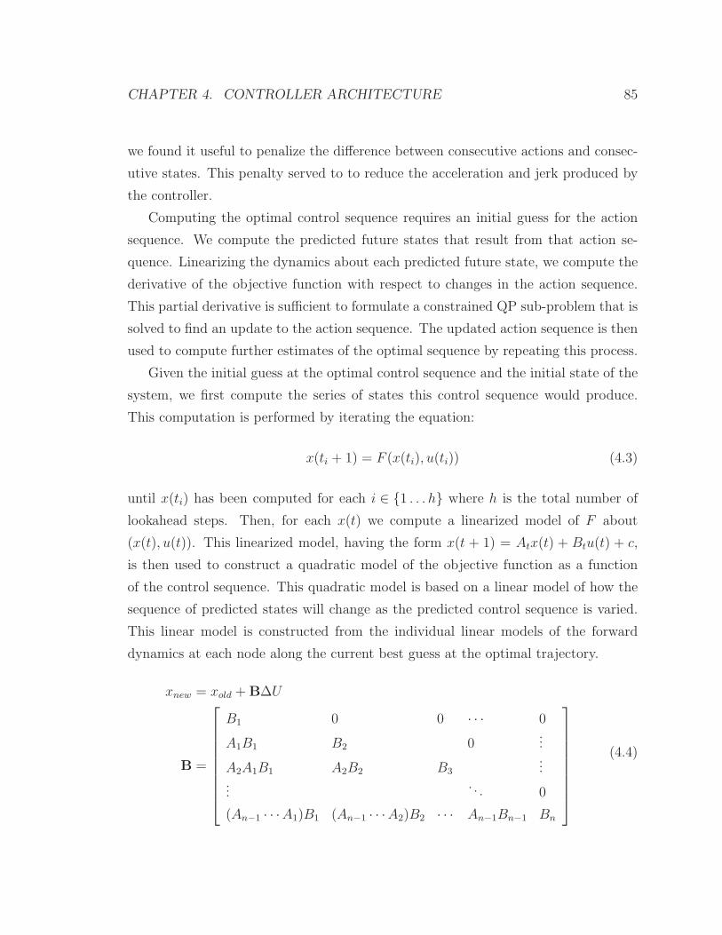
CHAPTER 4. CONTROLLER ARCHITECTURE 85
we found it useful to penalize the difference between consecutive actions and consec-
utive states. This penalty served to to reduce the acceleration and jerk produced by
the controller.
Computing the optimal control sequence requires an initial guess for the action
sequence. We compute the predicted future states that result from that action se-
quence. Linearizing the dynamics about each predicted future state, we compute the
derivative of the objective function with respect to changes in the action sequence.
This partial derivative is sufficient to formulate a constrained QP sub-problem that is
solved to find an update to the action sequence. The updated action sequence is then
used to compute further estimates of the optimal sequence by repeating this process.
Given the initial guess at the optimal control sequence and the initial state of the
system, we first compute the series of states this control sequence would produce.
This computation is performed by iterating the equation:
x(ti + 1) = F (x(ti), u(ti)) (4.3)
until x(ti) has been computed for each i ∈ {1 . . . h} where h is the total number of
lookahead steps. Then, for each x(t) we compute a linearized model of F about
(x(t), u(t)). This linearized model, having the form x(t + 1) = Atx(t) + Btu(t) + c,
is then used to construct a quadratic model of the objective function as a function
of the control sequence. This quadratic model is based on a linear model of how the
sequence of predicted states will change as the predicted control sequence is varied.
This linear model is constructed from the individual linear models of the forward
dynamics at each node along the current best guess at the optimal trajectory.
xnew = xold +B∆U
B =
B1 0 0 · · · 0
A1B1 B2 0...
A2A1B1 A2B2 B3
......
. . . 0
(An−1 · · ·A1)B1 (An−1 · · ·A2)B2 · · · An−1Bn−1 Bn
(4.4)

CHAPTER 4. CONTROLLER ARCHITECTURE 86
Once this linear relationship has been computed, the full quadratic objective func-
tion model can be derived:
C(x,u+∆u) =(X + B∆U)TQ(X + B∆U)T + (U +∆U)R(U +∆U)
=∆UT(BTQB+R)∆U+(
UT(R+RT) +XT(Q+QT)B)
∆U+
XTQX + UTRU
(4.5)
The minimum of this quadratic function with respect to the constraints is computed
using a quadratic programming routine with linear constraints that limit the max-
imum distance from the reference pose and maximum action. The optimal update
to the control sequence is then added to the current control sequence, and the en-
tire process is repeated until the control sequence converges or an iteration limit is
reached.
4.10.1 System Models for Receding Horizon Control
The receding horizon control formulation described in the previous subsection does
not depend on the use of a full or reduced model of the system. However, using a
full model increases the size of the actions space dramatically, and increases the time
required to solve each QP sub-problem. The computational resources available did
not allow us to optimize a control sequence for the action space of the full robot
within one control cycle. We developed an alternate formulation for the receding
horizon controller that avoided the need for reduced model dynamics while keeping
the dimensionality of the action space small.
Because the pose controlled robot that the receding horizon controller controls
is passively stable in the actuated degrees of freedom, it can have a small set of
available actions and still be stable. We exploit this fact by selecting only a subset
of the eigenmodes of the system as the action space of available accelerations. We
manually selected one or two motions that reflected our understanding of the actions
humans used to perform the task. More detail on this process is available in section
3.7.

CHAPTER 4. CONTROLLER ARCHITECTURE 87
4.11 Mode Switching Control
While the receding horizon controller performed well in simulation, it performed
poorly on the physical hardware. Because the receding horizon approach depends
on the accuracy of its model of the system, we suspected that inaccurate parameters
for the reduced model of the system could be a significant factor. To further re-
duce the number of model parameters, we designed a mode switching controller that
limited the number of possible output actions to a finite set of states. This simplifica-
tion limits the amount of experimental training data needed to determine the model
parameters. In particular, we have a single linear model with only four states that
describes the system dynamics with a fixed body pose. The transition between out-
put poses is modeled with a second, independent, linear model. Our implementation
included only two output actions, and these actions were symmetric mirror images
of each other. This output representation reduced the parameter space for the entire
model to a pair of four by four matrices, one for the continuous dynamics as the robot
held a steady pose, and one that captured the transition between the steady poses.
We built a hybrid linear model of the dynamics from the full rigid body dynamics
by applying the finite difference algorithm described in section 3.4 to the simulated
the full body dynamics. For the continuous time model, where the body pose is fixed
and the bongo-board moves, we set the body’s initial pose equal to the output pose
and varied the initial state of the bongo-board. To build the model of the transition
between desired poses, we simulated 0.3 second periods, in which the desired body
pose shifted smoothly from the initial pose to the mirror image of that pose over the
first 0.1 seconds. This smooth shift was the same shift used in the actual controller
when a transition was triggered. We built a linear model of the transition function
by simulating from many initial bongo-board states and fitting a first order model to
the resulting data.
The task policy selected one of two possible postures and provided that posture as
input to the base policy. The postures we chose tipped the board to the left or right,
without moving the center of mass. Because the state space was small we used a grid
based dynamic programming policy generation method to build a globally optimal

CHAPTER 4. CONTROLLER ARCHITECTURE 88
Start of Mode Switch
End of Mode Switch
State Mirroring
Continuous Dynamics
(Fixed Pose)
1
43
2
1 2 3 4
Figure 4.10: Hybrid Linear Dynamics
switching policy for this model.
Figure 4.10 describes a possible steady state behavior of the simulated hybrid
linear controller. Beginning with the state labeled one, the robot maintains a fixed
body pose as the board and roller move. A linear model of this system is simulated
with a time step of 0.01 seconds and at each timestep the decision policy may choose
to initiate a mode switch action. The continuous time dynamics (dashed blue line)
take the system through state two and eventually reach state three. When the system
reaches the decision boundary (gray region) the policy initiates a mode switch action
(state three). When the mode switch action occurs the desired pose shifts smoothly
to the mirror image of the initial pose over 0.1 seconds. The mode switch is modeled
as a single linear transform applied to the current state and represents 0.3 seconds of
elapsed time (solid red line). The additional 0.2 second after the desired pose reaches

CHAPTER 4. CONTROLLER ARCHITECTURE 89
the new fixed pose allows the robot’s body state to settle after the transition. After
the 0.3 second transition is complete, the system is in state four, which is the mirror
image of state one. To simplify the dynamic programming problem, we then invert
the state variables, effectively mirroring the system from left to right, and continue
the continuous time simulation.
Our first task when building the controller was to determine whether or not this
hybrid linear model had any stable orbits. In particular, we wanted to know if stable
orbits existed given pessimistic assumptions about model and sensor error. The pes-
simistic assumption we made was that following each transition action, the true state
of the system could be any state within the grid cell containing the point predicted
by the forward dynamics. This state uncertainty would persist until the system made
another transition. A state is not viable if there is no time at which all trajectories
originating from the vertices of the grid cell containing that state are passing through
other viable grid cells. The requirement that all vertex-originating trajectories be in
viable cells at the same time is required to build a control policy that determines the
time to wait before switching control outputs under the uncertainty conditions we
impose. To find the viable region, we iteratively update viability over all grid cells
until reaching a steady state. Even with the pessimistic assumption that the worst
possible transition would always be taken, we found a viable region in the simplified
model. Unfortunately, this viable region was very thin — applying PCA to the set of
viable grid cells revealed that it has nearly zero extent in the direction of the unstable
eigenmode.
The hybrid linear model was used as the basis for designing a switching policy that
chose when to initiate a transition between the two basic body poses. We wanted to
maximize the robustness of the policy, so we used a minimax dynamic programming
method to design the policy. We represented the policy on a grid, but instead of
choosing whether or not to begin a transition in each grid cell, we chose how long to
delay before starting a transition in each cell. We chose the time that minimized the
maximum cost of a transition, over the set of trajectories beginning at the vertices of
the current cell.
V (x) = min{t}∞
0
{C(x, t) + β
[
max{i}16
1
{V (xi(t))}
]
}
CHAPTER 4. CONTROLLER ARCHITECTURE 90
Where xi(t) is the trajectory starting at the ith vertex of the policy grid cell centered
on x, V (x) is the value function being computed, and C(x, t) is the cost of moving
along the trajectory beginning at x for t seconds, then executing a transition to the
other pose. The cost matrices Q and R used to compute the cost of both continuous
movement along a trajectory and the discrete transition function are produced by the
model reduction procedure, and derive directly from the full-model cost function.
Requiring that the elapsed time before the mode switch be identical for each mode
maximizes the insensitivity of the resulting policy to sensor error. The alternative,
in which the optimal transition time for each trajectory exiting a cell is selected
independently, assumes that the system is able to correctly identify the precise state
of the system, rather than only the nearest cell vertices. Coupling the decision times
for nearby trajectories results in a policy that selects actions that are viable regardless
of the precise initial state. This alternate formulation would be written as
V (x) = max{i}16
1
{min{t}∞
0
{C(x, t) + βV (xi(t))}}
4.12 Summary
This chapter described the two control architectures we developed to support dynamic
balance tasks with humanoids. The first, policy mixing control, combined the control
signals from several independent controllers using a single QP optimization step. This
softened that hard constraints found in strict priority control schemes, at the cost of
the ability to reason clearly about the stability of the aggregate system. The second
architecture, informed priority control, uses a serial cascade pattern to connect several
controllers, but uses automatic model generation to build a new model at each stage
of the cascade, allowing model based controllers to adapt their behavior based on the
configuration of the controllers consuming their output. This preserves the ability to
reason about the stability of the aggregate system, while allowing sub-controllers to
modify their behavior based on the behavior of other sub-controllers.
Chapter 5
Modeling and Sensing Error
The ability to accurately predict future states of the system is essential to our model
based controllers. This ability depends both on developing and maintaining an accu-
rate model of the robot and accurate estimation of the current state of the system.
The system model includes both the conversion from sensor raw signals to meaning-
ful units, and the rigid body model of the robot. The sensor signals that require
conversion to calibrated units are the joint position sensors, the joint load cells, the
six-axis foot load cells, and the valve command signals. The physical model of the
robot is a parametric rigid body model based initially on a CAD model of the robot.
This chapter describes the methods we used to identify best-fit parameters for the
mass, center of mass position, and moment of inertia for each link in the body based
on collected data. In addition to determining offline model parameters, we estimated
both model parameters and state online. This chapter also discusses how these online
adjustments were performed.
5.1 Kinematic Calibration
The first stage of our model parameter identification process was to build a kinematic
model of the robot. Based on the CAD model supplied by Sarcos, and verifying that
model with our own measurements, we constructed an initial kinematic model. The
Sarcos biped senses joint angles using linear plastic-film potentiometers, which provide
91

CHAPTER 5. MODELING AND SENSING ERROR 92
excellent linearity and a scale factor that does not vary significantly over time. We
needed to calibrate the linear scaling and zero-offset of these position sensors to sense
accurate joint angles. Additionally, because the zero offsets tended to shift over time,
we used a combination of an initial calibration procedure that established both the
scaling coefficients and the zero-offsets, and an on-line recalibration procedure that
corrected for drift in the zero-offsets.
5.1.1 Initial Calibration
We performed initial kinematic calibration using accelerometers fixed to the robot’s
feet and legs. With the hip fixed to a rigid stand we were able to measure the
difference in the observed gravitational acceleration between the first and last links
of each leg. We moved each joint in a sinusoidal trajectories to explore the space of
possible configurations. To avoid redundant configurations, we chose frequencies for
the sinusoidal trajectories that were prime relative to each other. To minimize the
error in the measurement of the gravity vector, we limited the maximum acceleration
of the feet by using a maximum sinusoidal trajectory frequency of 0.1Hz.
Once the acceleration data was collected we used a nonlinear optimizer [Gill et al.,
2002] to establish values for the linear coefficients and zero-offsets that best recon-
structed the observed data from the accelerometers. The objective function used for
the optimization was the sum-squared difference between the predicted and observed
accelerations at the distal accelerometer relative to the proximal accelerometer. The
results of this optimization process can be seen in figure 5.1.
5.1.2 On-line kinematic recalibration
While the scaling coefficients for the calibration were stable over long periods of time,
the zero-offsets for the position sensors shifted frequently. These zero-offset shifts
caused errors in foot placement or center of mass position estimation on the order
of a few centimeters. To correct this error, we developed a procedure to quickly
recalibrate the zero offsets for the lower body. This procedure used a wooden jig
that reliably positioned each foot at one of several locations by pressing two of its

CHAPTER 5. MODELING AND SENSING ERROR 93
Figure 5.1: Observed and predicted accelerations at the foot after nonlinear optimiza-tion of the kinematic calibration parameters. Horizontal scale is sample index at 0.1Hz. Pitch and roll are measured in radians. G is gravity vector projected onto Z axis.
edges against raised registration surfaces. We placed the feet at a sequence of known
locations and recorded the joint sensor readings and hip accelerometer gravitational
acceleration at each pose. Note that even with the feet fixed in known locations the
hip can still move freely in six dimensions. To find the zero offsets, we minimized
a cost function representing observation error over possible zero-offsets. This cost
function was the weighted sum of the difference between the predicted and known
position of the feet and the predicted and observed gravitational accelerations at the
hip. The values resulting from this optimization produced reliable updates to the
zero-offsets of the position sensors.

CHAPTER 5. MODELING AND SENSING ERROR 94
5.2 Load Calibration
Mechanical loads were measured using strain gauges attached at both the joint ac-
tuator linkages and the feet. The joint strain gauges measured strain in the linkage
between the hydraulic piston and the rotational joint, and could be used to recon-
struct joint torques. The foot strain gauges measured six-axis forces and torques
between the foot sole plates and the outboard ankle body. We developed separate
procedures for calibrating the joint and foot sensors.
5.2.1 Joint load sensors
We calibrated the joint loads by applying known torques to the joints and recording
the resulting strain gauge excitations. These torques were applied with a hand-held
strain gauge (IMADA DPS-44) connected to the same logging system that recorded
the bridge excitations. We attached the hand-held strain gauge to a known location
on the robot’s body with a length of filament and used the tension on this filament to
produce a test torque while the robot held a fixed position using an integral controller.
Using a filament, instead of directly pushing on the robot with the strain gauge,
reduced errors due to the angle of force applied. With a sufficiently long filament the
error in the force angle due to a given offset in the position of the strain gauge can be
made very small, as illustrated in figure 5.2. This figure shows that when a filament is
used, a much larger position error is needed to produce the same error in the effective
torque arm. The error in the effective torque arm is the difference between r and r′.
For each joint we recorded the sensor readings that resulted from four applied
forces with different magnitudes, then used a least squares regression to find the
scaling factor and zero-offset that best matched the observations. For the ankle
joints, where the robot’s physical structure does not provide an outboard point at
a distance sufficient to generate large torques, we clamped a board to the robot’s
foot, and attached the strain gauge filament to this board in order to generate large
torques about the ankle.

CHAPTER 5. MODELING AND SENSING ERROR 95
r
r’
r
r’
Figure 5.2: (left) Pressing the strain gauge directly onto the robot to produce a torqueis sensitive to the orientation of applied force and the alignment between the appliedforce vector and the strain gauge. (right) Using a filament to connect the strain gaugeto the robot reduces sensitivity to positioning error and aids alignment between thesensor axis and the applied force axis.
5.2.2 Foot load sensors
The foot sensors each contain eight strain gauge bridges and measured the six elements
of the wrench applied by the ground to the inboard ankle body. Calibrating the foot
load cells required the identification of a matrix with six rows and eight columns that
transforms bridge excitations into foot wrenches. We used a calibrated six-axis force
plate (Equitest MSA-6810) to measure the wrench applied to the robot’s foot. We
clamped the foot to a known location on the force plate, then applied forces to the
inboard ankle body that caused matching loads to be applied to both the foot load
cells and the Equitest force plate. We recorded both the calibrated wrench applied to
the force plate and the excitation voltages at each of the eight strain gauge bridges,
then computed the calibration matrix that minimized the reconstruction error in the
excitation.
If the strain gauges were perfectly linear, the full calibration matrix would not be
observable, because the number of strain gauges exceeds the number of dimensions
in the observation space. Sensor noise and other small nonlinearities can cause the
parameter matrix identification to be numerically unstable, because the extra degrees
of freedom are used to try to fit this noise. To make the computation more robust,
CHAPTER 5. MODELING AND SENSING ERROR 96
we included a hand-tuned ridge regression term that penalized selecting regression
coefficients far from zero. Without this ridge regression term very large coefficients
appeared in the solution due to the redundant bridges.
5.3 Model Identification
We identified the parameters of the robot’s rigid body model by collecting data from
the robot and then computing offline updates to these parameters that minimized
the difference between expected and observed sensor readings. Because the dynamics
are linear in the parameters [An et al., 1988], we were able to use singular value
decomposition to solve for the best parameters. By setting small singular values to
zero, we changed only the parameters that were well determined by the available
data.
By bolting a 5.76kg mass to a known position at the end of each leg and repeating
the trajectories used for position calibration, we were able to simultaneously calculate
the load cell scale factors for each joint, and the masses and first mass moment
parameters of the rigid body model, as well as the calibration matrices for the foot load
cells. Because the joint and foot load cell parameters had already been determined,
we performed the model fit twice, once with the load cell scale factors, and once
without. We were able to confirm that the model fit produced scale factors similar
to those we had found with our per-joint procedure. Ultimately, we chose to use the
model parameters produced by fixing the scale factors to the per-joint calibration
values.
After completing the leg calibration with the robot’s hip fixed to the rigid stand,
we performed additional model calibration with the robot standing freely. We moved
the robot through a sequence of postures while standing, and recorded both joint
torques and contact forces. We extended the method described by [An et al., 1988]
to include the additional parameters for load cell sensor calibration and a constant
external force applied by the umbilical. Figure 5.3 shows the resulting agreement
between the joint torques predicted by the model and those reported by the load
cells. This graph shows the hip and knee flexion torques as the robot slowly moves

CHAPTER 5. MODELING AND SENSING ERROR 97
Time (seconds)
Torq
ue
(N
m)
Figure 5.3: Observed and predicted torques at the hip and knee after mass model fit
all joints through co-prime sinusoidal trajectories.
5.4 Model Adaptation
Error in predicting future states, particularly errors in contact forces, center of mass
location, and total body momentum, can severely impact the performance of our
model based controllers. We experimented with several techniques intended to reduce
these errors. This section describes the techniques we used to adapt the parametric
model of the robot to the conditions we encountered in each trial. We first describe
model adaptations that were applied to the full model of the robot, then describe
adaptations that were applied to the lumped mass model. For each model type, we

CHAPTER 5. MODELING AND SENSING ERROR 98
describe separately the adaptations that were constant during the entire trial and the
adaptations that varied continuously during the trial.
5.4.1 Full model
Constant model adaptations
The predicted right hand side forces can have significant errors. Possible sources of
these errors are external forces applied by the umbilical tether and gravitational load
error due to inaccuracies in the model of the robot’s mass distribution. We developed
a technique to compensate for the zero-order components of these errors. Each trial
begins with the robot at rest. In this state we know that both q and q are zero. The
joint and contact loads, τ and λ, are directly observable, and can be used to compute
an observed right hand side force using those values:
RHSobs = Sτ + JcTλ
RHSerr = RHSmdl(q, q)−RHSobs
M(q)q + JcTλ+ Sτ = RHSmdl −RHSerr = RHSobs
We then subtract RHSerr from the right hand side forces when computing the inverse
dynamics constraints during the trial. When the robot is in the initial pose and the
expected acceleration is zero the commanded joint torques will be those that actually
produce zero acceleration. This offset makes switching to a model based controller
from an initial stance pose controller much more benign, because if the initial desired
acceleration is zero then there will be no instantaneous change in desired joint torques.
Modifying the mass matrix, M, can make model based control more robust to
error. The modifications we experimented with were adding a constant offset to the
diagonal and scaling the diagonal or off-diagonal elements of the mass matrix.
The first type of model error is the presence of unmodeled torques introduced
by joint stiction, pressurized hydraulic lines that cross joints, and errors in the rigid
body model parameters. If a particular joint has a small generalized inertia, then the
torque that the model predicts is necessary to achieve normal accelerations may be
CHAPTER 5. MODELING AND SENSING ERROR 99
small relative to these unmodeled disturbance forces. Adding a constant offset to the
diagonal of the mass matrix increases the output torques required to achieve desired
accelerations, and has a proportionally greater effect on low inertia joints.
We can show that adding a term to the diagonal of the mass matrix is approxi-
mately equivalent to adding a PD torque gain policy to the joint torques selected by
the policy mixer:
q = −Kacc
[
q q]T
[M+ cI] q = RHS − Sτ − JcTλ
Mq = RHS − Sτ − JcTλ+ cK
[
q q]T
Mq ≈ RHS − S
(
τ + cK[
q q]T)
− JcTλ
where cK is the PD gain matrix that is approximately equivalent to offsetting the
mass matrix by cI.
The off-diagonal elements of the mass matrix indicate the dynamic coupling be-
tween degrees of freedom in the system. By reducing the magnitude of these elements
of the matrix, we bias the system towards under-compensating for these couplings.
This decision also tends to make the system behave more like a pure decoupled PD
servo policy. We found that scaling the off-diagonal terms in the mass matrix could
increase the stability of some inverse-dynamics based policy mixing controllers.
By tuning both the scaling and offset parameters, we were able to access a con-
tinuous space of control solutions that range from model based inverse dynamics to
decoupled PD torque servos. In practice, for our experiments, we found that an offset
of 3kgm2
radand no scaling of the off-diagonal terms produced the best behavior on the
seesaw task with a policy mixing controller. We used these mass matrix manipula-
tion techniques only with the policy mixing controllers, not with the informed priority
controllers.

CHAPTER 5. MODELING AND SENSING ERROR 100
Time-varying model adaptations
During dynamic balance tasks, controlling contact forces precisely is more important
than controlling joint accelerations precisely. Additionally, because forces are sensed
directly, unlike accelerations, we can adapt to force errors faster. We minimize contact
force errors at the expense of joint acceleration errors by computing the contact force
model error λerr = λobs−λexp, where λobs is the current force and torque readings from
the foot load cells, and λexp is the expected contact force computed from the current
joint torques. Integrating λerr and projecting it into joint coordinates produces a
right hand side offset:
τerr = CλJcT∑
λerr
We add τerr to the right hand side forces in the inverse dynamics computation be-
fore solving for x. The error integration converges such that the expected contact
forces match the observed contact forces. In our experiments, the constant value Cλ
ranged from 0.01 to 0.001 with a 1kHz control rate. This value results in an effective
bandwidth ranging from 10Hz to 1Hz. We determined Cλ by searching for the largest
value that did not create oscillation, then reducing that maximum value by at least
half to arrive at the value used during the experiments.
5.4.2 Simplified models
Because the reduced model state drives the high level control actions, errors in the
estimation of this state can have the most significant effects on performance. We de-
veloped state estimation techniques that focus specifically on estimating the reduced
model state accurately.
Constant model adaptations
When using a single mass model the position and velocity of the center of mass are
computed using the rigid body model of the robot. Using this model to predict
the center of pressure while the robot is at rest can result in errors of two or three
centimeters. We use two techniques to improve the center of mass model. First, we
CHAPTER 5. MODELING AND SENSING ERROR 101
observe the center of pressure when the trial begins, and compute a constant offset to
the center of mass estimate that places the center of mass over the center of pressure.
Second, using data from several quasi-static trials we compute off-line, a linear model
of the center of mass estimate error, and apply this scaling term to the center of mass
estimate in future trials. The estimated center of mass becomes:
pcom = Ecommcom(q) + ecom
Where pcom is the estimated center of mass, Ecom is the linear model of center of
mass error computed from several earlier trials, and ecom is the center of mass offset
computed at the beginning of each trial.
Time-varying model adaptation
With the policy mixing controller, we used Kalman filters to compute the time-
varying error in the single mass model. A separate Kalman filter is used for the
coronal and sagittal planes. The Kalman filter estimates the center of mass position,
velocity, as well as the difference between the observed center of mass and the true
center of mass. This estimate of model error is treated as an additional state, but
is assumed to be constant except for process noise. The observations provided to
the filter are the position and velocity of the center of mass computed from q and q
using the rigid body model, and the location of the center of pressure. The process
and measurement covariances matrices are tuned so that the response time of the
error estimate is approximately 0.5 seconds. This value is the lowest we could achieve
without creating oscillation due to feedback between the control system and the model
adaptation.

Chapter 6
Experimental Results
This chapter discusses the experimental results from our seesaw balance and bongo-
board balance tasks. For the seesaw task, we review the experimental setup, then
show data collected from trial runs of the task, and finally discuss the significance
of these results. We verify that expected properties of policy mixing control were
present, and discuss the need for online model adaptation when working with the
robot hardware. In the bongo-board results section, we describe the robustness of
the controller in simulation and its failure to balance using the hardware. We provide
an analysis of why the controller failed in hardware, concluding that the contact
dynamics between the force plate and the bongo-board’s roller could have introduced
a small error in the estimation of the roller position that would have been sufficient
to destabilize the system.
6.1 Seesaw Balance
We demonstrate that our policy mixing controller is capable of performing the seesaw
balance task and responding to unexpected external disturbances. We also show that
the model adaption methods we described in chapter 5 are essential parts of this
controller, without which it does not function. This section begins with a description
of the hardware and software configuration used to perform the seesaw balance ex-
periments, then presents the experimental procedures used for each set of trials, and
102
CHAPTER 6. EXPERIMENTAL RESULTS 103
finally discusses the results of those experiments.
6.1.1 Experimental Setup
In our experiments, the robot stood on the seesaw and either maintained its balance in
the presence of unexpected pushes, or rocked the seesaw from side to side by moving
its center of mass. In some trials, unexpected pushes were applied to either the robot’s
body or to the seesaw. The feet were not fixed to the board, but were prevented from
sliding outward by raised ridges at the ends of the board. These ridges are intended
to assist repeatable placement of the robot’s feet on the board, rather than to prevent
foot sliding. In all the experiments, we used a 3DM-GX2 IMU to sense the angle and
velocity of the seesaw.
The software configuration we used for the experiments actively controlled only
the fourteen joints in the lower body. The upper body was controlled by a stiff PD-
servo policy that maintained a nearly constant pose. The initial postures for both the
upper and lower body were found by manually tuning joint positions until the robot
balanced statically on the seesaw while one end of the board rested on the ground.
We weighted the contact load, posture, and single-mass policies to give priority to
the single mass policy and the contact load policy. The single-mass policy attempted
to control the robot’s center of mass motion in both the sagittal and coronal planes.
The contact load policy prevented the edges of the feet from lifting off the ground by
keeping the center of pressure withing the area of support for each foot.
6.1.2 Trials
Our first trial was to slowly shift the desired position of the center of mass. This
objective was achieved by slowly changing the desired center of mass position in the
lumped mass balance policy. As it tracked the desired position, the center of mass
would pass over the rotational axis of the seesaw. When this event occurred the
seesaw rotated until the opposite end struck the ground.
When we performed this trial, we found that as the robot compensated for the
board’s unexpected rotation, it caused the board to move back to the left. Then, as

CHAPTER 6. EXPERIMENTAL RESULTS 104
the desired center of mass continued to move to the right, the board shifted one final
time, and came to rest with its right end on the ground. To provide some hysteresis,
we moved the desired center of mass slightly further to the right when the board was
tipped to the right. The online Kalman center of mass estimator (section 5.4.2) and
contact force integrator (section 5.4.1) were both essential to the success of this trial.
Their performance is shown in figure 6.2.
In the second and third trials, we manually forced the seesaw to move by pushing
on the board. In the second set of trials, we forced it remain in place for a period of
time. In the third set, we immediately allowed it to return to the left. The robot was
able to accommodate these unexpected disturbances, as seen in the accompanying
video and figure 6.3.
We also experimented with removing each of our model adaptation techniques
individually. We found that removing some model adaptations led to immediate
failure. These adaptations were the initial full model and reduced model RHS force
offsets, and the inertia matrix diagonal offset. Removing any of the online model
adaptation techniques resulted in failure once the system was perturbed.
6.1.3 Discussion
We were surprised that such extensive online correction was required, given the ap-
parent success of the offline model identification procedure. However, because the
balance controller must bring the center of mass close to the edge of the contact
region, balance can fail due to center of mass errors on the order of only a few cen-
timeters. Considering that the magnitudes of the errors introduced by umbilical hose
forces and mass model errors are on the order of a few centimeters, the need for these
additional corrective measures is not unreasonable.
For example, suppose that the hydraulic umbilical is applying 40N of lateral force
to the robot. This force is representative of the lateral force magnitude we have
observed when the robot is standing unsupported on a calibrated force plate. Because
the only connection between the robot and its environment are the umbilical and the
force plate, and non-gravitational force observed by the force plate must be due to
CHAPTER 6. EXPERIMENTAL RESULTS 105
the hose forces. With a body weight of about 900N, this lateral load will cause a
center of pressure displacement of slightly more than four centimeters.
In a static trial, the center of mass position estimator will converge to estimating
that the center of mass is located directly above the observed center of pressure. This
error-integrating behavior causes the single-mass sub-policy to eventually drive the
observed center of pressure to its desired position. Because there is an offset between
the true center of mass and the center of pressure, the expected steady state center
of mass displacement is four centimeters.
A calibration error in the ankle zero-offset on the order of 0.02 radians would also
be typical for our robot. Given a center of mass height of 0.8 meters this error results
in an additional two centimeter mass displacement. Six centimeters error in the center
of mass location is easily enough to destabilize the robot during normal balance, and
explains the need for online model error correction even given a completely accurate
offline mass model.
As we predicted, policies with larger weights dominated the output, while policies
with smaller weights operated primarily in the null space of these high-weight policies.
Figure 6.1 shows that low weight policies had larger differences between their desired
and actual control outputs than did the higher weight policies. For example, the
lumped mass policy’s error is expressed in terms of the moment about the desired
center of pressure. When the policy’s desired output is achieved exactly, this value
will be zero. During the trial, the moment about the desired center of pressure had
a maximum magnitude of 0.02N. Given a typical surface normal load on the order of
900N, this moment represents an expected center of pressure displacement of less than
a millimeter. By contrast, the difference between the low-weight joint torque policy’s
desired left ankle flex torque and the applied torque had a maximum magnitude of
about 50N. A 50N change in ankle torque corresponds to roughly a 5cm displacement
in the center of pressure location. This result is consistent with finding a torque
output that minimizes the weighted action error∑
i wiUerri .
Finding values for the Kalman filter process and noise covariance matrices that
produced fast convergence without oscillation, tuning the contact force integration
constant, and selecting the full body PD servo gains all required significant trial

CHAPTER 6. EXPERIMENTAL RESULTS 106
and error. Selecting these values was difficult because the stiffness and damping of
the balance and full body controllers determines how quickly the error estimators
can be allowed to converge without oscillating, and vice-versa. This interdependence
is another example of tight coupling between the offline configuration of separate
components of the control architecture.
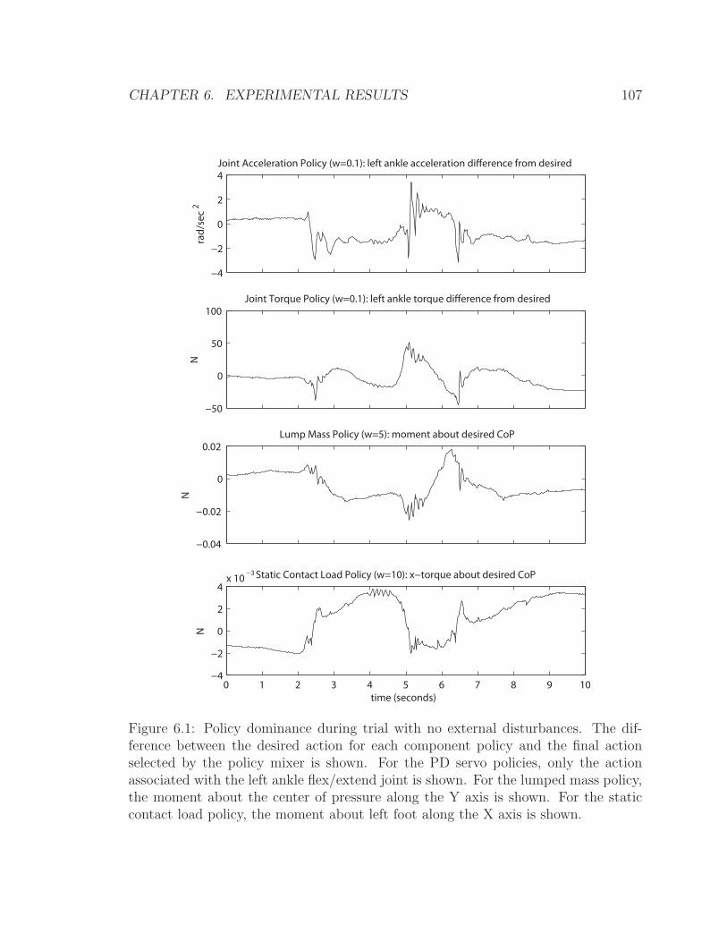
CHAPTER 6. EXPERIMENTAL RESULTS 107
−4
−2
0
2
4
rad
/se
c2
Joint Acceleration Policy (w=0.1): left ankle acceleration di!erence from desired
−50
0
50
100
N
Joint Torque Policy (w=0.1): left ankle torque di!erence from desired
−0.04
−0.02
0
0.02
N
Lump Mass Policy (w=5): moment about desired CoP
0 1 2 3 4 5 6 7 8 9 10−4
−2
0
2
4x 10
−3 Static Contact Load Policy (w=10): x−torque about desired CoP
N
time (seconds)
Figure 6.1: Policy dominance during trial with no external disturbances. The dif-ference between the desired action for each component policy and the final actionselected by the policy mixer is shown. For the PD servo policies, only the actionassociated with the left ankle flex/extend joint is shown. For the lumped mass policy,the moment about the center of pressure along the Y axis is shown. For the staticcontact load policy, the moment about left foot along the X axis is shown.
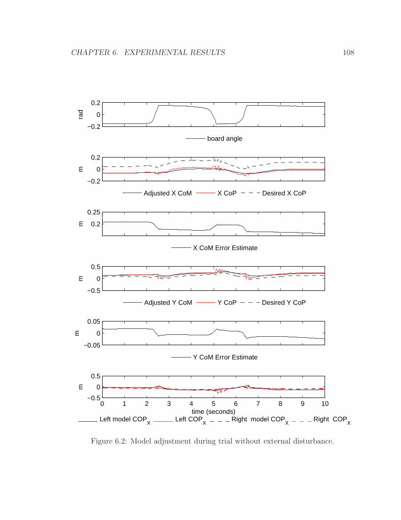
CHAPTER 6. EXPERIMENTAL RESULTS 108
−0.2
0
0.2
rad
board angle
−0.2
0
0.2
m
Adjusted X CoM X CoP Desired X CoP
0.2
0.25
m
X CoM Error Estimate
−0.5
0
0.5
m
Adjusted Y CoM Y CoP Desired Y CoP
−0.05
0
0.05
m
Y CoM Error Estimate
0 1 2 3 4 5 6 7 8 9 10−0.5
0
0.5
m
time (seconds)
Left model COPX
Left COPX
Right model COPX
Right COPX
Figure 6.2: Model adjustment during trial without external disturbance.

CHAPTER 6. EXPERIMENTAL RESULTS 109
−0.2
0
0.2
rad
−0.2
0
0.2
m
0
0.1
0.2
m
−0.5
0
0.5
m
−0.02
0
0.02
m
0 5 10 15 20 25 30−0.5
0
0.5
m
time (seconds)
board angle
Adjusted X CoM X CoP Desired X CoP
X CoM Error Estimate
Adjusted Y CoM Y CoP Desired Y CoP
Y CoM Error Estimate
Left model COPX
Left COPX
Right model COPX
Right COPX
Figure 6.3: Model adjustment during external disturbance.
CHAPTER 6. EXPERIMENTAL RESULTS 110
6.2 Bongo-Board Balance
We conducted balance experiments with a bongo-board setup that included addi-
tional sensors intended to simplify the control problem. The bongo-board’s roller
was constructed using a 6 inch diameter section of PVC pipe with three strips of
high-friction grip-tape applied on equally spaced radial bands. The bongo-board’s
board was constructed from 3
8inch birch plywood reinforced with 1 by 2 pine strips
fastened along each edge of the board. These strips also provided a hard stop for
positioning the robot’s feet on the board in a repeatable position. The bongo-board
was placed on a six axis force plate that continuously measured the load applied by
the roller. This load was used to compute the center of pressure on the force plate.
Ideally, that center of pressure lies along the line of contact between the roller and
plate, and indicates the position of the roller during balance.
We also experimented with hard rubber and soft foam coverings for both the force
plate and the bottom of the board. These coverings increase friction, eliminating
unwanted stick-slip yaw motion between roller and force plate or board and roller.
The coverings also change the dynamics of the bongo-board task, adding damping,
slowing down roller motion, and increasing the roller torque needed to initiate roller
motion.
The force plate used in our experiments was an AMTI Accusway. The analog
signal from this force plate was amplified and digitized by an AMTI MSA-6 amplifier
and processed at 200Hz by the control system.
6.2.1 Bongo-Board Simulation
In section 4.5, we described the informed priority control system for a Sarcos hu-
manoid balancing on a bongo-board. This controller used two sub-policies. The
task-level policy used a receding horizon controller based on a single linear model of
the system. The inner policy was a linear feedback, gravity compensated, pose con-
troller. This inner policy was designed to generate well damped responses to changes
in the desired pose and to minimize the expected acceleration error due to scaling
errors in torque outputs.
CHAPTER 6. EXPERIMENTAL RESULTS 111
We tested the receding horizon controller using both full-state and reduced-state
models of the system. The reduced-state model used two features of the full model as
its state. These features were the lateral center of mass displacement and the bongo-
board roller displacement. The board angle relative to the body was controlled,
but not include in the system state. We limited the available action space to one
or two dimensions, depending on the trial. For the action space basis, we selected
low-inertia modes of the forward dynamics that changed the board angle and roller
position without significantly altering the robot’s center of mass.
The receding horizon controller used between ten and seventeen collocation points
spaced at 0.2 second intervals. Using the reduced action space, the controller was
able to produce control outputs in less than 1 millisecond given a good initial guess
supplied to the QP solver. The previous solution for predicted action sequence worked
well as this initial guess. We selected a reference pose by optimizing for joint angles
that placed the center of mass over the roller while minimizing distance from the
basic stance pose and maintaining the kinematic contact constraints. An exponential
decay term was used to reduce the cost of states and actions that occurred further
in the future. This decay term helped to reduce rapid changes in the current torque
output due to predicted events far in the future.
6.3 Results
The simulated robot was able to balance successfully in trials using a range of control
parameters and simulated model errors. We varied the cost functions used in the
receding horizon controller, as well as the node spacing and look-ahead time. Ad-
ditionally, we varied the stiffness and damping of the pose controller. Finally, we
simulated constant offsets in the mass model and external disturbance forces to eval-
uate the effect these errors had on the performance of the system. These results can
be viewed in the video included with this thesis.
The damping of the pose controller significantly affected the success of the overall
controller. With excess damping the pose response was slow, and the system was
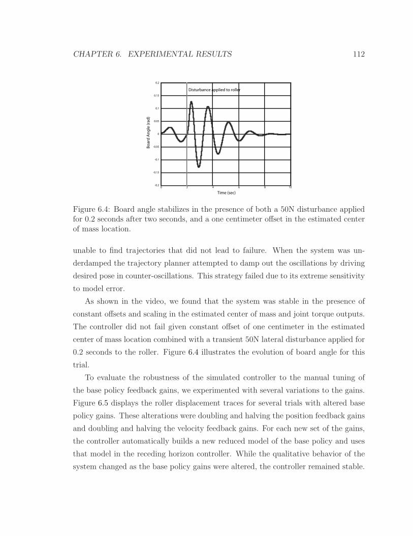
CHAPTER 6. EXPERIMENTAL RESULTS 112
-0.2
-0.15
-0.1
-0.05
0
0.05
0.1
0.15
0.2
0 2 4 6 8 10
Bo
ard
An
gle
(ra
d)
Time (sec)
Disturbance applied to roller
Figure 6.4: Board angle stabilizes in the presence of both a 50N disturbance appliedfor 0.2 seconds after two seconds, and a one centimeter offset in the estimated centerof mass location.
unable to find trajectories that did not lead to failure. When the system was un-
derdamped the trajectory planner attempted to damp out the oscillations by driving
desired pose in counter-oscillations. This strategy failed due to its extreme sensitivity
to model error.
As shown in the video, we found that the system was stable in the presence of
constant offsets and scaling in the estimated center of mass and joint torque outputs.
The controller did not fail given constant offset of one centimeter in the estimated
center of mass location combined with a transient 50N lateral disturbance applied for
0.2 seconds to the roller. Figure 6.4 illustrates the evolution of board angle for this
trial.
To evaluate the robustness of the simulated controller to the manual tuning of
the base policy feedback gains, we experimented with several variations to the gains.
Figure 6.5 displays the roller displacement traces for several trials with altered base
policy gains. These alterations were doubling and halving the position feedback gains
and doubling and halving the velocity feedback gains. For each new set of the gains,
the controller automatically builds a new reduced model of the base policy and uses
that model in the receding horizon controller. While the qualitative behavior of the
system changed as the base policy gains were altered, the controller remained stable.

CHAPTER 6. EXPERIMENTAL RESULTS 113
0 5 10 15−0.06
−0.04
−0.02
0
0.02
0.04
0.06
0.08
Time (seconds)
Rol
ler
disp
lace
men
t (m
eter
s)
NormalUnderdampedOverdampedIncreased P GainDecreased P Gain
Figure 6.5: Roller displacement traces for several different base policy gain selections.Both position and velocity terms were doubled and halved independently.
CHAPTER 6. EXPERIMENTAL RESULTS 114
Robustness to model error was of particular interest to us. We ran twenty trials
in which the mass of each link was altered during only the model building phase. The
altered masses were uniformly distributed within twenty five percent of their original
values. The result of this change is that while all the simulations used an identical
model, the model presented to the receding horizon controller varied in each trial
and did not match the simulated model. In only one of the simulations did this mis-
match result in failure, although several simulations converged slowly or to different
steady state behaviors. It is important to note that while these model errors alter
the predicted future behavior of the system (the A and B matrices in the linearized
dynamics), they do not alter the observed state of the reduced model.
6.3.1 Mode Switching Control
We replaced the receding horizon control component with the mode switching con-
troller described in section 4.11. The intent in performing this replacement was to
make the control system more robust to sensor and model error in determining the
system center of mass position. The controller interpolated smoothly between two
output actions over a fixed time period. Once a transition was initiated no further
transitions could be initiated until the first transition completed. Transition time was
fixed at 0.3 seconds. The two output actions were a pair of mirror image poses that
corresponded to tipping the board to the left and right without moving the center of
mass.
We used a planar decision surface to initiate the output transition, rather than the
grid based policy generated by the dynamic programming procedure. We derived the
parameters for this decision surface using both a hand-tuned experimental process and
the hybrid linear model described in section 4.11. We found that the policy produced
by the grid based dynamic programming solution to the hybrid linear system was
closely approximated by a planar decision surface, and that its parameters were very
close to those derived by hand-tuning. We used a support vector machine to compute
max-margin parameters for this plane. Both sets of decision surface parameters are
listed in table 6.1.

CHAPTER
6.
EXPERIM
ENTALRESULTS
115
0 5 10 15−0.1
−0.05
0
0.05
0.1
Time (seconds)Rol
ler
disp
lace
men
t (m
eter
s)
0 5 10 15−0.05
0
0.05
Time (seconds)
Rol
ler
angl
e (r
adia
ns)
Figure 6.6: In each trial the mass of each body used to build the model has been altered by a uniformly distributedamount up to 25 percent of the simulated value.
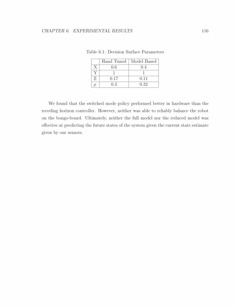
CHAPTER 6. EXPERIMENTAL RESULTS 116
Table 6.1: Decision Surface Parameters
Hand Tuned Model BasedX 0.6 0.4Y 1 1Z 0.17 0.11ρ 0.3 0.32
We found that the switched mode policy performed better in hardware than the
receding horizon controller. However, neither was able to reliably balance the robot
on the bongo-board. Ultimately, neither the full model nor the reduced model was
effective at predicting the future states of the system given the current state estimate
given by our sensors.

CHAPTER 6. EXPERIMENTAL RESULTS 117
6.4 Failure Analysis
Given that the task-level controller did not exhibit asymptotic stability in hard-
ware, we wanted to understand what factors might have contributed to the difference
in stability between simulation and hardware. To develop this understanding, we
conducted several experiments in simulation. Each experiment added an additional
element to the simulation that we suspected may have contributed to the failure in
hardware. These additional elements included several sensing delays and sensing er-
rors introduced by the roller-floor contact area. While all these elements were capable
of destabilizing the simulation when configured aggressively, most did not produce
a failure mode that reflected the failures we observed in hardware. Only the roller-
floor contact area simulation produced the characteristic low frequency bang-bang
control output we encountered in the hardware controller. Moreover, it produced this
effect for very conservative tunings of the simulation, suggesting that the task-level
bongo-board controller is very sensitive to this particular effect.
In hardware we had observed three distinct failure modes, two of which we were
able to resolve with appropriate tuning. These first two were high frequency oscillation
of the body pose, which was resolved by turning down the pose tracking damping
gains. The second was increasing low frequency oscillations of the reduced order
system, essentially the roller and center of mass would oscillate side to side two or
three times, with the magnitude of the oscillation growing until failure. This second
failure mode was resolved by tuning the pose controller to respond faster, but in
doing so a third failure mode was encountered. In this mode, the output action
oscillated at 3-7 Hz between its limits, eventually becoming unstable. Examples
of these failure modes from hardware trials are shown in figures 6.7 and 6.8 (high
frequency mode), figures 6.9 and 6.10 (bang-bang mode), and figures 6.11 and 6.12
(increasing oscillation mode).
Our initial hypothesis was that phase lag in the pose controller was causing the
predicted and observed behavior of the reduced model system to diverge. The reduced
model is built using the assumption that the body pose is precisely equal to the desired
body pose, without respect to how quickly the desired body pose is changing. This
CHAPTER 6. EXPERIMENTAL RESULTS 118
assumption is violated when the pose controller cannot precisely track the desired
pose produced by the task controller. The result of violating this assumption is that
the reduced model system no longer behaves according to the model built using the
assumption of perfect tracking.
The first step in testing this hypothesis was to verify that violating the assumption
that the pose tracked the desired pose precisely produced significant changes in the
evolution of the reduced model state. To test this assumption we conducted two
simulated trials that began with identical reduced model state (i.e. the roller and the
center of mass in identical locations) and used a constant pose control input, but
had different initial body postures. In the first trial, the initial body pose matched
the constant desired pose exactly, while in the second trial a neutral initial pose that
did not match the desired pose was chosen. The initial reduced model state for both
trials was identical, and the task-level control input was identical, but the systems
behaved differently while the desired and actual poses did not match. This result is
shown in figures 6.13 and 6.14.
Having established that pose tracking performance could have a significant im-
pact on the behavior of the reduced model system we conducted additional trials
to determine whether the performance impacts of changing pose tracking behavior
produced the specific failure modes we had observed in hardware. We augmented
the pose-control generation procedure described in section 4.6 with two additional
inputs. One input, Kp, scaled the output gain matrix linearly. The second input,
Ks, scaled the damping gains relative to the expected value needed to achieve critical
damping. By varying these two parameters, we were able to rapidly generate several
sets of gains with different tracking performance. We evaluated the performance of
these different gain configurations in their response to a step input in command sig-
nal. These results can be seen in figure 6.15, demonstrating that the range of gain
configurations significantly altered the time needed for the system to converge to the
desired pose, as well as secondary characteristics of the performance, such as over-
shoot and oscillation. To determine whether any of these gains produced changes in
performance that matched the hardware failure, we simulated the full controller using
each set of gains. We found that low gains produced slowly increasing oscillations

CHAPTER
6.
EXPERIM
ENTALRESULTS
119
0 1 2 3 4 5 6−0.05
−0.04
−0.03
−0.02
−0.01
0
0.01
0.02
0.03
0.04
0.05
seconds
met
ers
High Frequency Oscillation
RollerCoM
Figure 6.7: High Frequency Failure (State)

CHAPTER
6.
EXPERIM
ENTALRESULTS
120
0 1 2 3 4 5 6
−0.3
−0.2
−0.1
0
0.1
0.2
0.3
seconds
met
ers
High Frequency Oscillation
Desired Displacement
Figure 6.8: High Frequency Failure (Action)
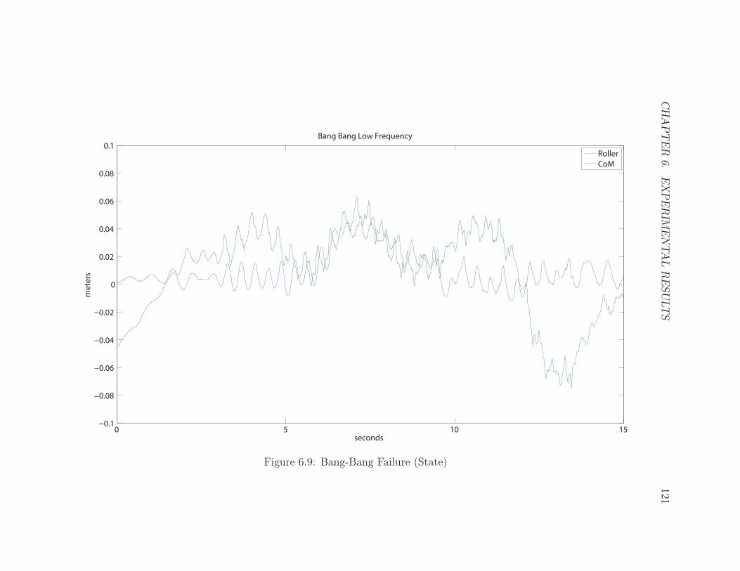
CHAPTER
6.
EXPERIM
ENTALRESULTS
121
0 5 10 15−0.1
−0.08
−0.06
−0.04
−0.02
0
0.02
0.04
0.06
0.08
0.1
Bang Bang Low Frequency
seconds
meters
Roller
CoM
Figure 6.9: Bang-Bang Failure (State)
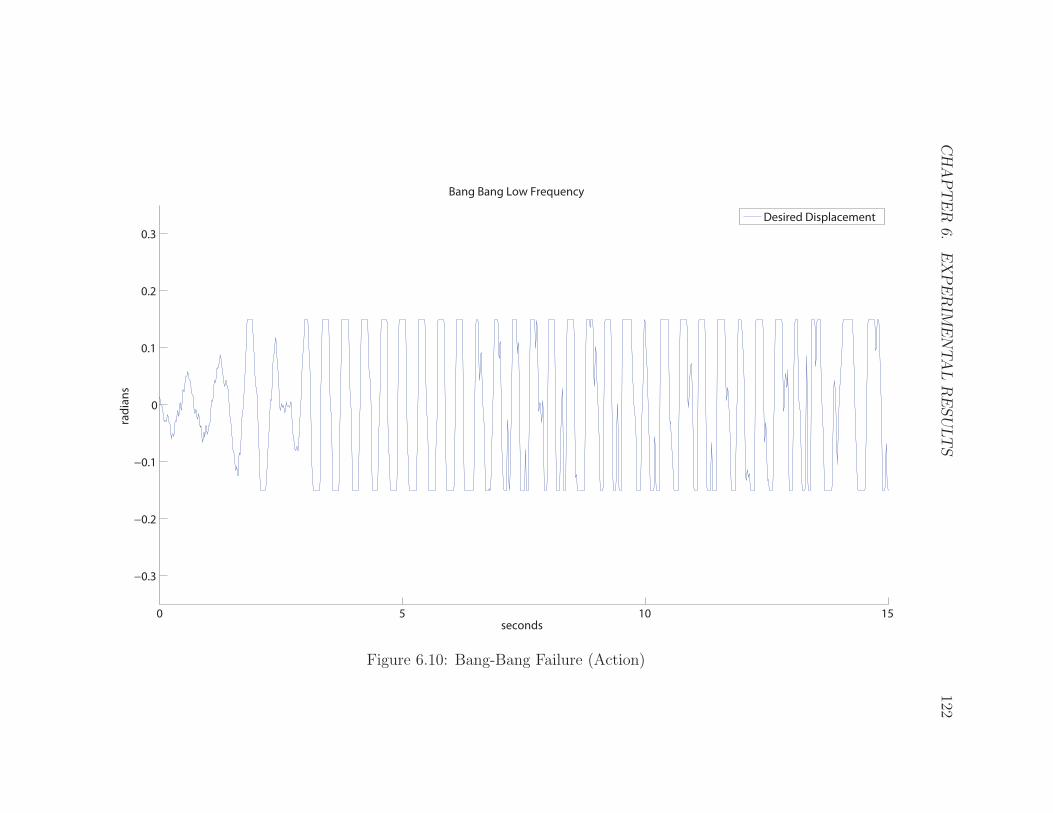
CHAPTER
6.
EXPERIM
ENTALRESULTS
122
0 5 10 15
−0.3
−0.2
−0.1
0
0.1
0.2
0.3
seconds
radians
Bang Bang Low Frequency
Desired Displacement
Figure 6.10: Bang-Bang Failure (Action)

CHAPTER
6.
EXPERIM
ENTALRESULTS
123
0 5 10 15−0.1
−0.08
−0.06
−0.04
−0.02
0
0.02
0.04
0.06
0.08
0.1
Increasing Oscillation
seconds
meters
Roller
CoM
Figure 6.11: Increasing Oscillation Failure (State)

CHAPTER
6.
EXPERIM
ENTALRESULTS
124
0 5 10 15−0.4
−0.3
−0.2
−0.1
0
0.1
0.2
0.3
0.4
seconds
radians
Increasing Oscillation
Desired Displacement
Figure 6.12: Increasing Oscillation Failure (Action). Clipping at -0.3 radians reflects software limits on outputcontrol signal.
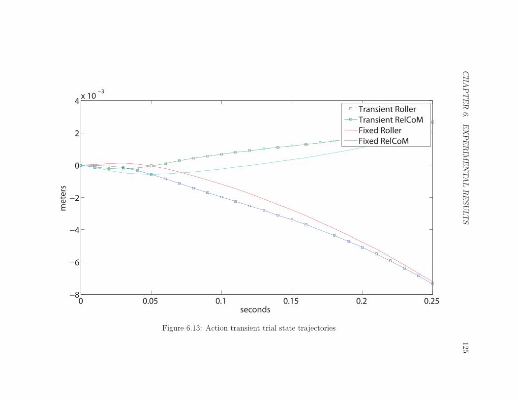
CHAPTER
6.
EXPERIM
ENTALRESULTS
125
0 0.05 0.1 0.15 0.2 0.25−8
−6
−4
−2
0
2
4x 10
−3
seconds
meters
Transient Roller
Transient RelCoM
Fixed Roller
Fixed RelCoM
Figure 6.13: Action transient trial state trajectories

CHAPTER
6.
EXPERIM
ENTALRESULTS
126
0 0.05 0.1 0.15 0.2 0.25−0.06
−0.05
−0.04
−0.03
−0.02
−0.01
0
0.01
0.02
0.03
0.04
seconds
meters
Transient Roller Vel
Transient RelCoM Vel
Fixed Roller Vel
Fixed RelCoM Vel
Figure 6.14: Action transient trial command trajectories

CHAPTER
6.
EXPERIM
ENTALRESULTS
127
0 0.1 0.2 0.3 0.4 0.5 0.6 0.7 0.8 0.9 10
0.05
0.1
0.15
0.2
0.25
0.3
0.35
0.4
Time (seconds)
Join
t dis
plac
emen
t alo
ng a
ctio
n ba
sis
(rad
ians
)
Pose Response For Multiple Gain Configurations
Kp=0.4, Sd=1 Response
Kp=1, Sd=1 Response
Kp=10, Sd=1 Response
Kp=10, Sd=0.5 Response
Kp=10, Sd=0.25 Response
Command
Figure 6.15: Variations in pose tracking behavior induced by choosing different gain tuning parameters. Thedisplacement value shown is the magnitude of the body pose projected onto the action basis vector.

CHAPTER 6. EXPERIMENTAL RESULTS 128
in the reduced model state, while gains that were tuned too stiffly produced unsta-
ble pose control at much higher frequencies (approximately 10Hz). These results are
shown in figures 6.16 and 6.17.
These results showed that values of Ks that were either too low or too high would
cause the system to fail. While we did observe both the slowly growing oscillations
that occurred with Ks = 1 and the high frequency pose control failure that occurred
when Ks = 0.5, neither of these exhibited the low-frequency bang-bang command
signal we encountered in hardware. These failures agree with our intuition about
how the value Ks should affect performance. Higher values of KS result in pose
controllers with longer transients, which make the task-level controller unable to
compensate quickly for errors, while lower values underdamp the pose controller and
lead to increasing high frequency oscillations. We attempted to produce the low-
frequency bang-bang failure mode by including additional features in the simulation.
A comparison between increasing oscillation failure in hardware and simulation is
shown in figures 6.18 and 6.19.
We introduced several additional features into the simulation and tested each
in isolation. These features were joint velocity signal delay, IMU velocity signal
delay, IMU position signal delay, and roller position error introduced by roller contact
dynamics with the force plate. Introducing signal delays easily destabilized the pose
controller, the task controller, or both, but the failures were similar to those we had
already observed in the gain configuration trials. The most significant difference
being that we could produce both the high-frequency pose controller oscillations and
the low frequency task-controller oscillations simultaneously. Figure 6.20 illustrates
the results of the signal delay trials. The most striking feature of these results is
that the system is relatively insensitive to delays in the IMU angular rate signal.
This observation produced the hypothesis that the reduced model state velocities
were determined largely by the force plate state signals, and that simulating errors
in these signals might produce the velocity-dependent bang-bang control outputs we
had seen in hardware.
The roller contacts the force plate through a layer of foam rubber that prevents
the roller from spinning around the vertical axis. As the force applied to the roller

CHAPTER
6.
EXPERIM
ENTALRESULTS
129
0 2 4 6 8 10−0.05
0
0.05
Ks = 1
seconds
radians
0 2 4 6 8 10−0.05
0
0.05
Ks = 0.5
seconds
radians
0 2 4 6 8 10−0.05
0
0.05
Ks = .75
seconds
radians
0 2 4 6 8 10−0.05
0
0.05
Ks = .6
seconds
radians
Roller
CoM
Figure 6.16: Four trials with varying effective damping. Kp was set to ten in each trial, but Ks varied from 0.5to 1. For low values of Ks the system responded quickly and the task-level controller damped out oscillations inthe reduced model state (e.g. Ks = 0.5, upper right), but the pose controller itself was unstable resulting in highfrequency pose oscillations.

CHAPTER
6.
EXPERIM
ENTALRESULTS
130
0 2 4 6 8 10
−0.3
−0.2
−0.1
0
0.1
0.2
0.3
Ks = 1
seconds
radians
0 2 4 6 8 10
−0.3
−0.2
−0.1
0
0.1
0.2
0.3
Ks = 0.5
seconds
radians
0 2 4 6 8 10
−0.3
−0.2
−0.1
0
0.1
0.2
0.3
Ks = .75
seconds
radians
0 2 4 6 8 10
−0.3
−0.2
−0.1
0
0.1
0.2
0.3
Ks = .6
seconds
radians
Desired Displacement
Pose Displacement
Figure 6.17: These plots show the pose command and pose displacement corresponding to the four trials shown infigure 6.16. They show that the system tracked the desired pose more closely in the trials where Ks was smaller.

CHAPTER
6.
EXPERIM
ENTALRESULTS
131
0 1 2 3 4 5 6 7 8−0.05
0
0.05
Simulation
seconds
meters
0 1 2 3 4 5 6 7 8−0.05
0
0.05
Hardware
seconds
meters
Roller
CoM
Figure 6.18: A comparison between the increasing low frequency oscillation failure mode in both simulation andhardware.

CHAPTER
6.
EXPERIM
ENTALRESULTS
132
23 24 25 26 27 28 29 30 31
−0.4
−0.2
0
0.2
Hardware
Action (radians)
0 1 2 3 4 5 6 7 8
−0.3
−0.2
−0.1
0
0.1
0.2
0.3
seconds
Action (radians)
Simulation
Desired Displacement
Pose Displacement
Figure 6.19: A comparison between the action trajectories in simulation and hardware in the increasing lowfrequency oscillation failure mode.

CHAPTER
6.
EXPERIM
ENTALRESULTS
133
0 2 4 6 8 10
−0.3
−0.2
−0.1
0
0.1
0.2
0.3
Joint Velocity Delay
seconds
radians
0 2 4 6 8 10
−0.3
−0.2
−0.1
0
0.1
0.2
0.3
IMU Position Delay
seconds
radians
0 2 4 6 8 10
−0.3
−0.2
−0.1
0
0.1
0.2
0.3
IMU Velocity Delay
seconds
radians
0 2 4 6 8 10
−0.3
−0.2
−0.1
0
0.1
0.2
0.3
Force Plate (Roller Position) Delay
seconds
radians
Desired Displacement
Pose Displacement
Figure 6.20: Four trials with various signal delays. In the upper left plot, the joint velocity was delayed by twentymilliseconds. In the upper right plot, the IMU orientation signal was delayed by four milliseconds. In the lower leftplot, the IMU angular rate signal was delayed by twenty milliseconds. The lower right plot shows the force platesignal delayed by ten milliseconds. Longer delays produced immediate failure in all cases.
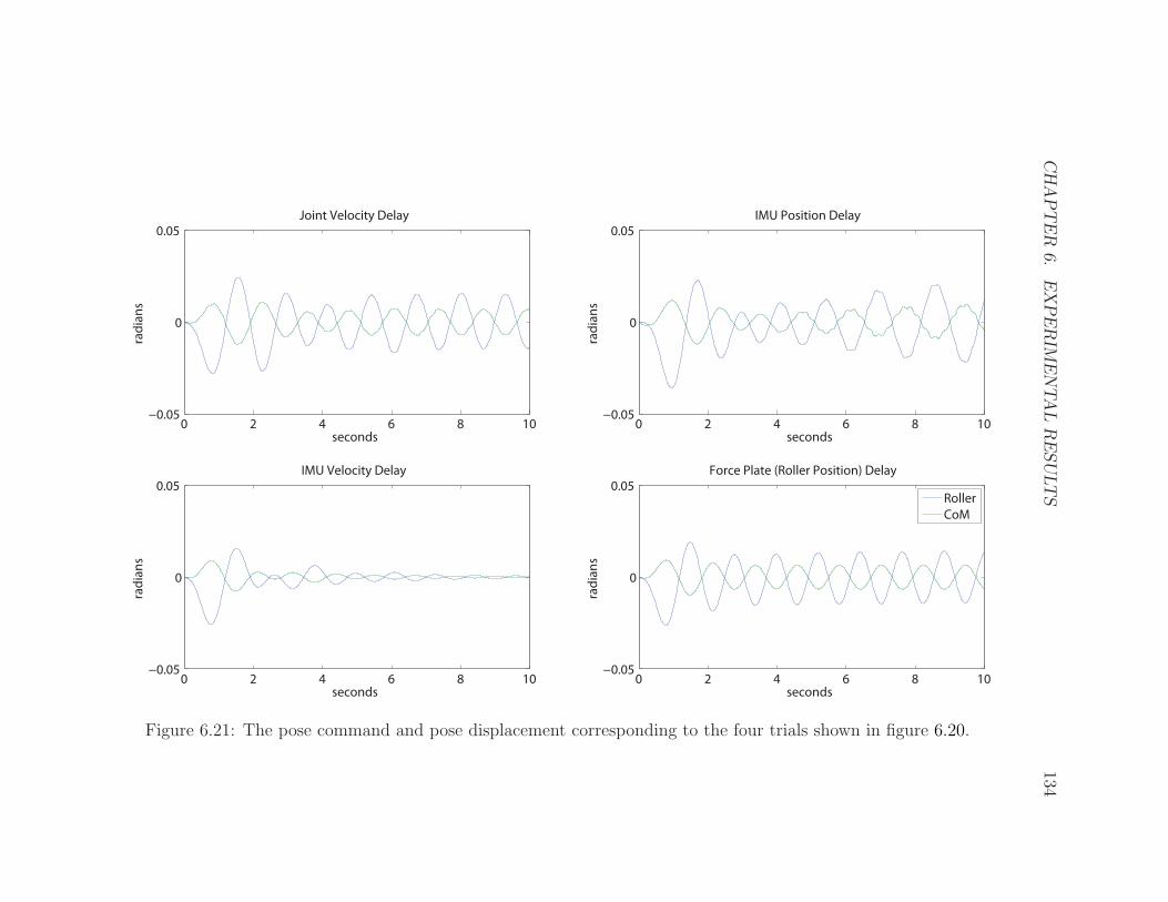
CHAPTER
6.
EXPERIM
ENTALRESULTS
134
0 2 4 6 8 10−0.05
0
0.05
Joint Velocity Delay
seconds
radians
0 2 4 6 8 10−0.05
0
0.05
IMU Position Delay
seconds
radians
0 2 4 6 8 10−0.05
0
0.05
IMU Velocity Delay
seconds
radians
0 2 4 6 8 10−0.05
0
0.05
Force Plate (Roller Position) Delay
seconds
radians
Roller
CoM
Figure 6.21: The pose command and pose displacement corresponding to the four trials shown in figure 6.20.

CHAPTER 6. EXPERIMENTAL RESULTS 135
by the board changes, the center of pressure can move away from the bottom of
the roller. We approximated this displacement in simulation by scaling the lateral
acceleration of the roller and using that value to offset the position signal recorded
from the simulated force plate. We used a scaling coefficient of 0.0025 s2, which yields
a position displacement of 5mm for an roller acceleration of 2ms2. In simulation, we
observed maximum roller accelerations of slightly less than 1.5ms2, so the maximum
absolute position error introduced by the simulation of this error is less than 5mm.
Simulating with a smaller scaling coefficient of 0.001 produced a stable simulation,
while 0.01 resulted in nearly immediate failure. The important feature of the failures
caused by the contact sensing simulation is that it matches the low frequency bang-
bang control output we saw in hardware.
Examination of the simulation data revealed that the roller’s lateral acceleration
was tightly coupled to the joint space displacement along the action basis, with the
data being well fit by a linear relationship with acceleration equal to 8.5 times the
basis excitation. This relationship completes a feedback loop which begins with the
roller velocity signal, which drives the control output, which in turn drives the pose
excitation, which directly alters the observed roller position, which changes the esti-
mated roller velocity. With a CoM velocity feedback gain of approximately 50 and
an output range of ±0.3 a velocity perturbation of 6mmsec
can drive the output over its
full range. This perturbation is within the range of the disturbance introduced by the
observed accelerations. Figure 6.22 illustrates the results of this simulation. Further
evidence for the roller position sensing error hypothesis is provided by a comparison
between the roller position sensed using motion capture and the roller position sensed
using the force plate. Using the larger diameter roller, we attached motion capture
markers to each end of the shaft running through the axis of the roller. A human
balanced on a bongo-board on the roller to simulate the contact forces experienced
during robot bongo-boarding. Both the motion capture marker positions and the
force plate readings were recorded simultaneously by the motion capture controller.
This configuration eliminated differences in time base between the two traces because
both signals were recorded on the same clock pulse. Figure 6.24 shows the difference
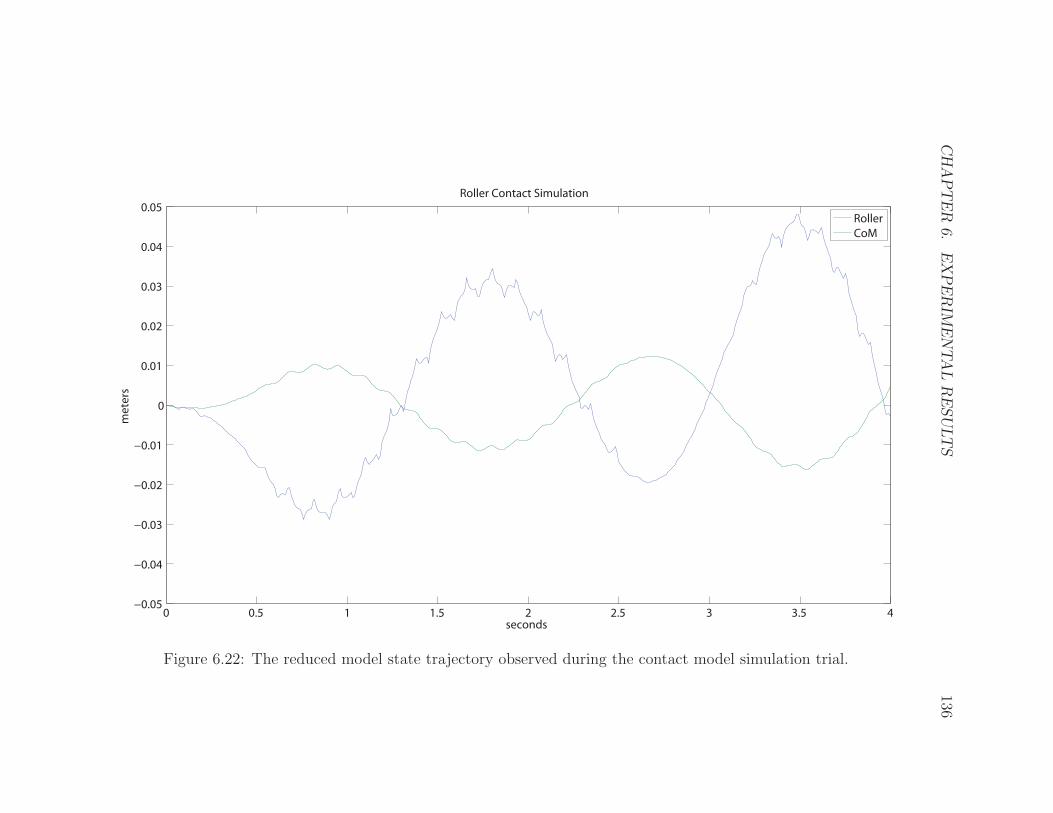
CHAPTER
6.
EXPERIM
ENTALRESULTS
136
0 0.5 1 1.5 2 2.5 3 3.5 4−0.05
−0.04
−0.03
−0.02
−0.01
0
0.01
0.02
0.03
0.04
0.05
Roller Contact Simulation
seconds
meters
Roller
CoM
Figure 6.22: The reduced model state trajectory observed during the contact model simulation trial.

CHAPTER
6.
EXPERIM
ENTALRESULTS
137
0 0.5 1 1.5 2 2.5 3 3.5 4
−0.3
−0.2
−0.1
0
0.1
0.2
0.3
Roller Contact Simulation
seconds
radians
Desired Displacement
Pose Displacement
Figure 6.23: Low frequency bang-bang control output produced by modeling the effects of contact dynamics onthe sensed roller position. The state trajectory for this trial is shown in figure 6.22.

CHAPTER 6. EXPERIMENTAL RESULTS 138
between these two traces. The error magnitude, shown in figure 6.25, was on the or-
der of 5mm. Fitting the error with a linear regression based on the roller acceleration
and velocity reduces the mean squared error from 4.7mm to 1.8mm.
While multiple failure modes are possible in simulation, and all of these modes can
be forced by introducing features that more accurately reflect the delays present in
hardware, only the model of the effect that contact dynamics have on the sensed roller
position produced the characteristic bang-bang control outputs we saw in hardware
when the system was tuned so that it did not produce either the high-frequency pose
control instability or the low-frequency increasing oscillations caused by slow response
times. Furthermore, our observation in hardware that lowering velocity feedback gains
and slowing down the response time of the pose controller helped to avoid entering
this failure mode is consistent with our observations in simulation. We conclude that
this error, and other potential unmodeled coupling between observed roller position
and commanded action are probably the root cause of poor performance in hardware.
In general, any unexpected motion of the roller caused by the commanded action
could produce similar perturbations in the roller velocity signal, with the potential
for similar feedback to occur.
6.4.1 Discussion
This failure analysis yields some insight into how our controller design methodology
might be improved. The surprising feature of the hardware failure is that it happened
despite the apparent robustness of the controller to model parameter and state esti-
mation error in simulation. Before moving to hardware, we demonstrated that our
reduced model learning procedure quickly converged to stable gains in simulation,
over a range of model parameter perturbations. Additionally, we had shown that
the controller was robust to the introduction of sensor error in the form of Gaussian
noise and constant offset, and to external perturbations. Despite this robustness, our
failure analysis shows that a particular type of a state estimation error could have
caused the failures we saw in hardware. Our earlier evaluation did not consider this
class of errors.
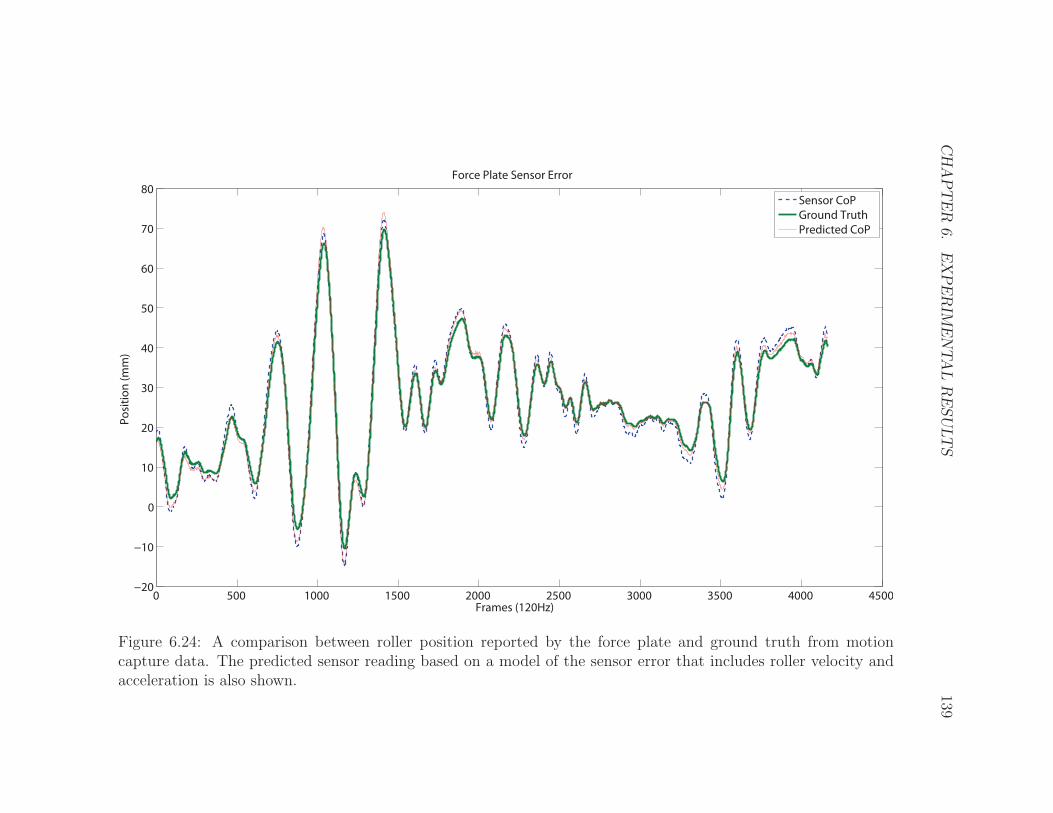
CHAPTER
6.
EXPERIM
ENTALRESULTS
139
0 500 1000 1500 2000 2500 3000 3500 4000 4500−20
−10
0
10
20
30
40
50
60
70
80
Force Plate Sensor Error
Frames (120Hz)
Position (mm)
Sensor CoP
Ground Truth
Predicted CoP
Figure 6.24: A comparison between roller position reported by the force plate and ground truth from motioncapture data. The predicted sensor reading based on a model of the sensor error that includes roller velocity andacceleration is also shown.
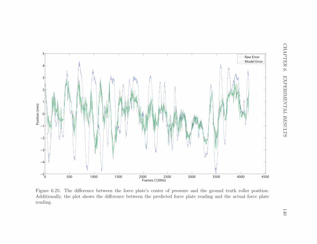
CHAPTER
6.
EXPERIM
ENTALRESULTS
140
0 500 1000 1500 2000 2500 3000 3500 4000 4500−5
−4
−3
−2
−1
0
1
2
3
4
5
Frames (120Hz)
Position (mm)
Raw Error
Model Error
Figure 6.25: The difference between the force plate’s center of pressure and the ground truth roller position.Additionally, the plot shows the difference between the predicted force plate reading and the actual force platereading.

CHAPTER 6. EXPERIMENTAL RESULTS 141
In our experience, the most difficult errors to correct are correlated disturbances
over time, because most of the robust control tools we use, like linear quadratic
regulators and Kalman filters, are designed to compensate for uncorrelated noise.
We compensated for some errors of this more difficult type with control features like
the acceleration variance minimizing gravity compensation torque solution, which
compensates for constant scaling errors in torque output, and tested our ability to
model and correct for other long-term sources of correlated error like model parameter
miscalibration. The coupling of the roller motion to the observed roller position was
not captured by any of these evaluations, and our controller proved to be very sensitive
to this particular type of error. This error is one of a large class of sensing errors in
which the observed state can be expressed as a linear function of the true state and
the control input. While our control formulation includes an observation matrix, we
did not learn its parameters from data, but supplied values based on earlier sensor
calibration.
It seems unlikely that the approach to state estimation we used could have pre-
vented this problem. Specifically, our Kalman filter based state estimator is designed
to be robust to uncorrelated white noise in sensor readings and state updates, but
does not include the possibility of an altered observation matrix that could be used
to represent the unmodeled roller position sensor error. This deficiency suggests two
changes to our methodology. First, we could attempt to learn a general model relat-
ing system state to sensor readings. Presently we refine the reduced model dynamics
based on experimental data, but it is possible that the observation matrix in our
linear system could also be fit to the data. Second, when evaluating failures, we as-
sumed that large discrepancies between the observed and predicted trajectories were
due to errors in the dynamic model, rather than in sensing. Adding an additional
source of ground truth data, for example a robust motion tracking system, could have
been used to disambiguate these two sources of error and to learn the values of the
observation matrix.
We did not use ground truth from motion capture because processing delays made
it difficult to incorporate into real-time control feedback. However, our failure analysis
suggests that it would have been an early way to detect our sensing errors if it had
CHAPTER 6. EXPERIMENTAL RESULTS 142
been used in an off-line capacity to verify the state estimation and sensor readings
we were using in the real time controller.
Future attempts at performing the bongo-board task in hardware could consider
forgoing the need to directly sense roller position. Humans are able to perform the
bongo-board task without directly observing the roller position, and report having
a strong sense of roller location while performing the task. This data suggests that
foot contact forces and body inertia provide enough information to infer the roller
position.
The control design we used in our trials provides several important features that
should be preserved in future attempts. First, it allows the control problem to be
decomposed into components that can be tested independently. The body pose con-
troller can be tested in standing balance, and then observed while supported on the
bongo-board to gather data that is used to refine the bongo-board reduced model
parameters. Once the pose-control component is tested the task-controller can be
implemented and tested independently. Several specific features of the pose con-
troller were also important to producing robust and compliant pose-control while on
the bongo-board. Representing gains in the space of the modes of the mass model
allowed us to quickly tune the behavior of the pose controller to produce the desired
compliance for the bongo-board task. The acceleration-variance minimizing gravity
compensation design and learned error correction term for gravity compensation were
important elements of producing a stable and compliant pose controller on the bongo-
board. The reduced model parameter learning methodology we used proved able to
adapt to significant changes in the mass model in simulation, and could be preserved
in a future approach that included more robust sensor error calibration.

Chapter 7
Conclusions
In this thesis, we described a method for designing and implementing humanoid
robot control systems. The control system design we developed was informed priority
control. Informed priority control uses a serial composition of two or more model
based controllers, and automates the generation of each model. In section 3.4, we
showed how approximate models for the system regulated by each controller could
be built using an automatic differentiation process, and discussed the limits of those
approximations.
Automating the generation of these models and controllers makes experimenting
with many reduced model representations feasible. We demonstrated that this exper-
imentation is important because the best choice for the reduced model of a system is
often non-obvious. In section 3.3.3, we showed that some plausible choices for reduced
models can result in unexpectedly poor performance. We also explained why the pre-
dominant work flow for designing controllers for humanoid robots, which begins with
the choice of a reduced model and builds the control system on top of that model, is
not well suited for rapid experimentation with alternative reduced models.
The implementation of a controller for the bongo-board task included several
techniques that were particularly important to producing a functioning controller.
Minimum variance gravity compensation (section 4.8) chose gravity compensation
torques that minimized unwanted accelerations due to scaling errors in the torque
output calibrations. Designing whole-body linear feedback gains using an eigenmode
143

CHAPTER 7. CONCLUSIONS 144
decomposition was an effective and practical way to produce a pose controller with
the response characteristics we wanted. Linear models of the error in the joint torque
estimate provided by the rigid body model (section 5.4.2) also allowed us improve the
match between predicted and observed joint torques at rest.
Finally, faced with divergent performance in simulation and hardware, we ana-
lyzed probable causes for the degraded hardware performance (section 6.4) . Using
simulations of possible sources of error, we discovered that the characteristic failure
behavior we observed could have been caused by the coupling between the lateral
load on the support surface and the sensor reading for the roller position. We also
established that the failures were most likely not due to improper tuning of the pose
controller’s behavior, or delays in the readings from various sensors.
This thesis has shown that the choice of reduced model representation for hu-
manoid control problems is an important factor in the performance of the control
system, and that most approaches to control system design in the literature require
significant effort to change the reduced model representation once a control system
has been implemented. The technique we suggest, informed priority control, reduced
the effort required to change reduced model representations. Additionally, we showed
that informed priority control, combined with other techniques discussed in this the-
sis, could be used to construct robust controllers in simulation.
Future Work
The automated model reduction technique developed for Informed Priority Control
can be applied in other contexts. Of particular interest is sub-dividing the policy
optimization stage of developing a SIMBICON style controller to reduce the number
of free parameters being optimized in each stage. For example, rather than simul-
taneously optimizing policy parameters for a full three dimensional walking biped,
a policy for an inverted pendulum walker based on a reduction of the full system
dynamics could be build first. That walker could be extended to a more complex
sagittal plane simulation and additional policy parameters introduced and optimized.
Finally, the full dynamics could be introduced and the full set of policy parameters
CHAPTER 7. CONCLUSIONS 145
optimized over. The links between these simplified models and the full system, as
well as the relationships between the control policies for the simplified models and the
full model could be expressed using the action inflation and state reduction functions
used by Informed Priority Control.
We have not developed in detail a technique that would allow Informed Priority
Control to update simplified models based on data collected from experiments. Be-
cause low dimensional models have fewer free parameters, they should require less data
to fit robustly than the full state dynamic model. Future work could explore the use
of experimental data, in either online or offline context, to update sub-system models.
Specifically, when sub-system configurations change, a technique that updated mod-
els based on experiments conducted with earlier configurations could eliminate the
need to re-collect experimental data describing sub-system performance after each
configuration change.
Finally, when developing the linear feedback component of the pose controller
for the bongo-board task we did not investigate using an LQR design process in
the mode space representation. It’s possible that this design would have simpli-
fied choosing the entries of the cost matrices, while using more information about
the model in choosing the gains than the direct gain tuning approach we used.

Bibliography
Pieter Abbeel, Varun Ganapathi, and Andrew Y. Ng. Learning vehicular dynamics,
with application to modeling helicopters. In Proc., Advances in Neural Information
Processing Systems (NIPS), 2006. 22
R. McN. Alexander. A model of bipedal locomotion on compliat legs. Philosophical
Transactions: Biological Sciences, 338(1284):189–198, October 1992. 3
Chae H. An, Christopher G. Atkeson, and John Hollerbach. Model-Based Control of
a Robot Manipulator. MIT Press, 1988. 22, 96
S. O. Anderson and J. K. Hodgins. Adaptive torque-based control of a humanoid
robot on an unstable platform. In Proc., IEEE Humanoids, Nashville, Tennessee,
2010. 13, 36, 56, 63
S. O. Anderson and J. K. Hodgins. Informed priority control for humanoids. In Proc.,
IEEE Humanoids, Bled, Slovenia, November 2011. 57
S. O. Anderson, M. Wisse, C. G. Atkeson, J. K. Hodgins, G. J. Zeglin, and B. Moyer.
Powered bipeds based on passive dynamic principles. In Proc., IEEE Humanoids,
pages 110–116, December 2005. 14
S.O. Anderson, C.G. Atkeson, and J.K. Hodgins. Coordinating feet in bipedal balance.
In Proc., IEEE Humanoids, pages 624 – 628, November 2006. 5, 29
Stuart O Anderson, Jessica K Hodgins, and Christopher G Atkeson. Approximate
policy transfer applied to simulated bongo board balance. In Proc., IEEE Hu-
manoids, 2007. 5
146
BIBLIOGRAPHY 147
A.C. Antoulas, D.C. Sorenson, and S. Gugercin. Structured Matrices in Mathematics,
Computer Science, and Engineering, volume 1, chapter A survey of model reduction
methods for large-scale systems. 2001. 27
T. Asfour, K. Regenstein, P. Azad, J. Schroder, A. Bierbaum, N. Vahrenkamp, and
R. Dillmann. ARMAR-III: An integrated humanoid platform for sensory-motor
control. In Proc., IEEE Humanoids, pages 169–175, Genova, Italy, December 2006.
18
C. G. Atkeson and J. Morimoto. Non-parametric representation of a policies and value
functions: A trajectory based approach. In Proc., Advances in Neural Information
Processing Systems (NIPS), volume 15, 2003. 16
C. G. Atkeson and B. Stephens. Random sampling of states in dynamic programming.
In Proc., Advances in Neural Information Processing Systems (NIPS), 2007. 16
C. G. Atkeson, A. W. Moore, and S. Schaal. Locally weighted learning. Artificial
Intelligence Review, 11:11–73, 1997a. 22, 75
Christopher G. Atkeson. Using local trajectory optimizers to speed up global opti-
mization in dynamic programming. In Jack D. Cowan, Gerald Tesauro, and Joshua
Alspector, editors, Proc., Advances in Neural Information Processing Systems, vol-
ume 6, pages 663–670. Morgan Kaufmann Publishers, Inc., 1994. 19
Christopher G. Atkeson, Andrew W. Moore, and Stefan Schaal. Locally weighted
learning for control. Artificial Intelligence Review, 11(1-5):75–113, 1997b. 22
J. Andrew Bagnell and Jess G. Schneider. Autonomous helicopter control using
reinforcement learning policy search methods. In Proc. International Conference
on Robotics and Automation (ICRA), May 2001. 22
J. Barbic, A. Safonova, J. Pan, C. Faloutsos, J. Hodgins, and N. Pollard. Segmenting
motion capture data into distinct behaviors. In Proc., Graphics Interface, 2004. 18
BIBLIOGRAPHY 148
Philippe Beaudoin, Michiel van de Panne, and Pierre Poulin. Automatic construction
of compact motion graphs. Technical Report 1296, DIRO, Universite de Montreal,
May 2007. 18
D.C. Bentivegna and C.G. Atkeson. Learning from observation using primitives. In
Proc., IEEE International Conference on Robotics and Automation (ICRA), pages
1988–1993, 2001. 11
R. Blickhan and R. J. Full. Similarity in multilegged locomotion: Bouncing like a
monopode. Journal of Comparative Physiology A: Neuroethology, Sensory, Neural,
and Behavioral Physiology, 173(5):509–517, November 1993. 59
M.S. Branicky, T.A. Johansen, I. Petersen, and E. Frazzoli. On-line techniques for
behavioral programming. In Proc., IEEE Conference on Decision and Control,
pages 1840–1845, 2000. 11
Thomas Buschmann, Sebastian Lohmeier, Mathias Bachmayer, Heinz Ulbrich, and
Friedrich Pfeiffer. A collocation method for real-time pattern generation. In Proc.,
IEEE Humanoids, 2007. 28
Min Gyu Choi, Jehee Lee, and Sun Yong Shin. Planning biped locomotion using
motion capture data and probabalistic roadmaps. ACM Transactions on Graphics
(SIGGRAPH 2003), 22(2):182–203, April 2003. 17
A. Dasgupta and Y. Nakamura. Making feasible walking motion of humanoid robots
from human motion capture data. In Proc., IEEE International Conference on
Robotics and Automation (ICRA), volume 2, pages 1044–1049, Detroit, MI, May
1999. 19
Kemalettin Erbatur and Utku Seven. An inverted pendulum based approach to biped
trajectory generation with swing leg dynamics. In Proc., IEEE Humanoids, 2007.
28
M. Erdmann and M. Mason. An exploration of sensorless manipulation. IEEE J.
Robot. Automat., 4(4), August 1988. 11

BIBLIOGRAPHY 149
A. Fang and N. Pollard. Efficient synthesis of physically valid human motion. In
ACM Transactions on Graphics, 22, 2003., 2003. 21, 62
Ray Fielding. Architectural Styles and the Design of Network-based Software Archi-
tectures. PhD thesis, University of California, Irvine, 2000. 53
A. Fod, M.J. Mataric, and O.C. Jenkins. Automated derivation of primitives for
movement classification. Autonomous Robots, 1:39–54, January 2002. 11
M. Garcia, A. Chatterjee, A. Ruina, and M. J. Coleman. The simplest walking model:
Stability, complexity, and scaling. ASME J. Biomech. Eng., 120(2):281–288, April
1998. 12, 59
P.E. Gill, W. Murray, and M.A. Saunders. SNOPT: An SQP algorithm for large-scale
constrained optimization. SIAM Journal on Optimization, 12(4):979–1006, 2002.
92
Jr. Golliday, C. and H. Hemami. An approach to analyzing biped locomotion dy-
namics and designing robot locomotion controls. IEEE Transactions on Automatic
Control, 22(6):963–972, December 1977. ISSN 0018-9286. 26
A. Goswami, B. Espiau, and A. Keramane. Limit cycles and their stability in a passive
bipedal gait. In Proc., IEEE International Conference on Robotics and Automation
(ICRA), Piscataway, NJ, 1996. 12, 59
Robert D. Gregg and Mark W. Spong. Reduction based control with application
to three-dimensional bipedal walking robots. In American Control Conference,
Seattle, Washington, 2008. 27
N. Hansen and A. Ostermeier. Adapting arbitrary normal mutation distributions in
evolution strategies: The covariance matrix adaptation. In Proc., IEEE Interna-
tional Conference on Evolutionary Computation, 1996. 15
J. K. Hodgins and M. N. Raibert. Adjusting step length for rough terrain locomotion.
IEEE Trans. Robotics and Automation, 7(3):289 – 298, 1991. 59

BIBLIOGRAPHY 150
J.K. Hodgins. Biped gait transitions. In Proc., IEEE International Conference on
Robotics and Automation, 1991. 59
S.H. Hyon. Compliant terrain adaptation for biped humanoids without measuring
ground surface and contact forces. IEEE Transactions on Robotics, 25(1):171–178,
2009. 7, 20
S.H. Hyon, JG Hale, and G. Cheng. Full-body compliant human–humanoid interac-
tion: balancing in the presence of unknown external forces. IEEE Transactions on
Robotics, 23(5):884–898, 2007. 12, 21
D.H. Jacobson and D.Q. Mayne. Differential Dynamic Programming. Elsevier, 1970.
62
Sumit Jain and C. Karen Liu. Modal-space control for articulated characters. ACM
Transactions on Graphics, 30:118:1–118:12, October 2011. 26, 27
Doug L. James and Kayvon Fatahalian. Precomputing interactive dynamic de-
formable scenes. ACM Transactions on Graphics (SIGGRAPH 2003), 22(3):879–
887, July 2003. 25
O.C. Jenkins and M.J. Mataric. Automated derivation of behavior vocabularies for
autonomous humanoid motion. In Proc., Autonomous Agents and Multi Agent
Systems, pages 225–232, 2003. 11
Odest C. Jenkins and Maja J Mataric. A spatio-temporal extension to isomap nonlin-
ear dimension reduction. In Proc., International Conference on Machine Learning,
pages 441–448, July 2004. 28
Shuuji Kajita, Fumio Kanehiro, Kenji Kaneko, Kiyoshi Fujiwara, Kensuke Harada,
Kazuhito Yokoi, and Hirohisa Hirukawa. Biped walking pattern generation by using
preview control of zero-moment point. In Proc., IEEE International Conference on
Robotics and Automation (ICRA), 2003. 4, 21, 28

BIBLIOGRAPHY 151
Jung-Yup Kim, Ill-Woo Park, and Jun-Ho Oh. Experimental realization of dynamic
walking of biped humanoid robot khr-2 using zmp feedback and inertial measure-
ment. Advanced Robotics, 20(6):707 – 736, June 2006. 19
Lucas Kovar, Michael Gleicher, and Frederic Pighin. Motion graphs. ACM Transac-
tions on Graphics, 21(3):473–482, July 2002. 18
James Kuffner, Koichi Nishiwaki, Satoshi Kagami, Masayuki Inaba, and Hirochika
Inoue. Motion planning for humanoid robots. In Proc. 11th Intl. Symp. of Robotics
Research, 2003. 17
J.J. Kuffner, S. Kagami, K. Nishiwaki, M. Inaba, and H. Inoue. Dynamically-stable
motion planning for humanoid robots. Autonomous Robots, 12(1):105–118, 2002.
21
Ryo Kurazume, Shuntaro Tanaka, Masahiro Yamashita, Tsutomu Hasegawa, and Kan
Yoneda. Straight legged walking of a biped robot. In Proc. IEEE/RSJ International
Conference on Intelligent Robots and Systems (IROS), 2005. 18
S. M. LaValle and J. J. Kuffner. Randomized kinodynamic planning. International
Journal of Robotics Research, 20(5):378–400, May 2001. 16
Steven M. LaValle. Rapidly-exploring random trees: A new tool for path planning.
Technical Report 98-11, Iowa State University, Ames, IA, 50011, USA, 1998. 16
Jehee Lee, Jinxiang Chai, Paul Reitsma, Jessica Hodgins, and Nancy Pollard. Inter-
active control of avatars animated with human motion data. ACM Transactions
on Graphics (SIGGRAPH 2002), 21(3), July 2002. 18
S. Levine, J. M. Wang, A. Haraux, Z. Popovi, and V. Koltun. Continuous char-
acter control with low-dimensional embeddings. ACM Transactions on Graphics
(SIGGRAPH 2012), 31(4), 2012. 18
C. Karen Liu and Zoran Popovic. Synthesis of complex dynamic character motion
BIBLIOGRAPHY 152
from simple animations. In SIGGRAPH ’02: Proc., Computer graphics and inter-
active techniques, pages 408–416, New York, NY, USA, 2002. ACM Press. ISBN
1-58113-521-1. 26
M. Vukobratovic and B. Borovac. Zero-moment point - thirty five years of its life.
Int. J. of Humanoid Robotics, 1(1):157–173, March 2004. 12
A. Macchietto, V. Zordan, and C. R. Shelton. Momentum control for balance. In
Transactions on Graphics, volume 28, 2009. 35
Arash Mahboobin, Patrick J. Loughlin, Mark S. Redfern, Stuart O. Anderson,
Christopher G. Atkeson, and Jessica K. Hodgins. Sensory adaptation in human
balance control: Lessons for biomimetic robotic bipeds. Neural Networks, 21(4):
621 – 627, 2008. ISSN 0893-6080. Robotics and Neuroscience. 23
M. Mason. The mechanics of manipulation. In Proc., IEEE International Conference
on Robotics and Automation (ICRA), volume 2, pages 544–548, March 1985. 11
M.J. Mataric, M. Williamson, J. Demiris, and A. Mohan. Behavior-based primitives
for articulated control. In Proc., Fifth Interational Conference on Simulation of
Adaptive Behavior, pages 165–170. MIT Press, 1998. 11
Microstrain, Inc. http://www.microstrain.com/, 2008. 6
M. Mistry, S. Schaal, and K. Yamane. Inertial parameter estimation of floating-base
humanoid systems using partial force sensing. In Proc., IEEE Humanoids, 2009.
22
M. Mistry, J. Buchli, and S. Schaal. Inverse dynamics control of floating base systems
using orthogonal decomposition. In Proc., International Conference on Robotics
and Automation (ICRA), 2010. 64
J. Morimoto, G. J. Zeglin, and C. G. Atkeson. Minimax differential dynamic program-
ming: application to a biped walking robot. In Proc., International Conference on
Intelligent Robots and Systems, volume 2, pages 1927 – 1932. IEEE, 2003. 58
BIBLIOGRAPHY 153
J. Morimoto, Sang-Ho Hyon, C. G. Atkeson, and G. Cheng. Low-dimensional feature
extraction for humanoid locomotion using kernel dimension reduction. In Proc.,
IEEE International Conference on Robotics and Automation (ICRA), pages 2711–
2716, Pasadena, CA, 2008. 25, 28
David D. Morrison, James D. Riley, and John F. Zancanaro. Multiple shooting
method for two-point boundary value problems. Commun. ACM, 5(12):613–614,
1962. ISSN 0001-0782. 61
Bilge Mutlu, Fumitaka Yamaoka, Takayuki Kanda, Hiroshi Ishiguro, and Norihiro
Hagita. Nonverbal leakage in robots: communication of intentions through seem-
ingly unintentional behavior. In Proc., ACM/IEEE International Conference on
Human Robot Interaction, 2009. 10
J. Nakanishi, M. Mistry, and S. Schaal. Inverse dynamics control with floating base
and constraints. In Proc., IEEE International Conference on Robotics and Au-
tomation (ICRA), pages 1942–1947, 2007. 21, 64
Jonghoon Park and Youngil Youm. General zmp preview control for bipedal walking.
In Proc., IEEE International Conference on Robotics and Automation, 2007. 26,
56
N. S. Pollard and P. S. A. Reitsma. Animation of humanlike characters: Dynamic
motion filtering with a physically plausible contact model. In Proc., Yale Workshop
on Adaptive and Learning Systems, 2001. 18, 20, 21
Zoran Popovic and Andrew Witkin. Physically based motion transformation. In
SIGGRAPH, pages 11–20. ACM, 1999. ISBN 0-201-48560-5. 28, 33
M. H. Raibert. Legged robots that balance. The MIT Press, Cambridge, Massachusetts,
1986. ISBN 0-262-18117-7. 14, 56, 59
John Rebula, Fabian Ca nas, and Jerry Pratt. Learning capture points for humanoid
push recovery. In Proc., IEEE Humanoids, 2007. 28
BIBLIOGRAPHY 154
C. Rose, M. F. Cohen, and B. Bodenheimer. Verbs and adverbs: multidimensional
motion interpolation. IEEE Computer Graphics and Applications, 18(5):32–40,
September/October 1998. ISSN 0272-1716. 18
L. Saab, N. Mansard, F. Keith, J-Y. Fourquet, and P. Soueres. Generation of dynamic
motion for anthropomorphic systems under prioritized equality and inequality con-
straints. In Proc., IEEE International Conference on Robotics and Automation
(ICRA), pages 1091–1096, 2011. 56
Alla Safonova, Nancy S. Pollard, and Jessica K Hodgins. Optimizing human motion
for the control of a humanoid robot. In Proc., International Symposium on Adaptive
Motion of Animals and Machines (AMAM2003), March 2003. 18, 19
Alla Safonova, Jessica K Hodgins, and Nancy Pollard. Synthesizing physically realistic
human motion in low-dimensional, behavior-specific spaces. ACM Transactions on
Graphics (SIGGRAPH 2004), 23(3), August 2004. 18, 25, 26, 28
E. Schuitema, D. G. E. Hobbelen, P. P. Jonker, M. Wisse, and J. G. D. Karssen.
Using a controller based on reinforcement learning for a passive dynamic walking
robot. In Proc., IEEE Humanoids, pages 232–237, December 2005. 58
Adam L. Schwartz. Theory and Implementation of Numerical Methods Based on
Runge-Kutta Integration for Solving Optimal Control Problems. PhD thesis, Uni-
versity of California at Berkeley, Berkeley, CA, 1996. 61, 62
L. Sentis and O. Khatib. A whole-body control framework for humanoids operating
in human environments. Proc., IEEE International Conference on Robotics and
Automation (ICRA), pages 2641–2648, May 2006. ISSN 1050-4729. 12
Luis Sentis. Synthesis and Control of Whole-Body Behaviors in Humanoid Systems.
PhD thesis, Stanford University, 2007. 58
Hyun Joon Shin and Jehee Lee. Motion synthesis and editing in low-dimensional
spaces. Computer Animation and Virtual Worlds (Special Issue: CASA 2006), 17
(3-4):219 – 227, July 2006. 28
BIBLIOGRAPHY 155
Takaaki Shiratori, Shunsuke Kudoh, Shin’ichro Nakaoka, and Katsushi Ikeuchi. Tem-
poral scaling of upper body motion for sound feedback system of a dancing hu-
manoid robot. In Proc., IEEE/RSJ International Conference on Intelligent Robots
and Systems (IROS), 2007. 19
J. D. Simon and S. K. Mitter. A theory of modal control. Information and Control,
13:316–353, 1968. 26
Kwang Won Sok, Manmyung Kim, and Jehee Lee. Simulating biped behaviors from
human motion data. ACM Transactions on Graphics, 26(3):105:1–105:10, July
2007. 19
R. F. Stengel. Optimal Control and Estimation. Dover, New York, 1994. 61
B. Stephens. Push Recovery Control for Force-Controlled Humanoid Robots. PhD
thesis, Carnegie Mellon University, August 2011. 12, 35
B. J. Stephens and C. G. Atkeson. Dynamic balance force control for compliant
humanoid robots. In Proc., IEEE/RSJ International Conference on Intelligent
Robots and Systems (IROS), pages 1248–1255, 2010. 55
Benjamin Stephens. Dynamic balance force control for compliant humanoid robots.
In Proc., International Conference on Intelligent Robots and Systems (IROS), 2010.
12
Yuval Tassa, Tom Erez, and William D. Smart. Receding horizon differential dy-
namic programming. In Proc., Advances in Neural Information Processing Systems
(NIPS), 2007. 19, 62
J.A. Ting, M. Mistry, J. Peters, S. Schaal, and J. Nakanishi. A bayesian approach
to nonlinear parameter identification for rigid body dynamics. In Proc., Robotics:
Science and Systems. Citeseer, 2006. 22
G. Venture, K. Ayusawa, and Y. Nakamura. Dynamics identification of humanoid
systems. In Proc. CISM-IFToMM Symp. on Robot Design, Dynamics, and Control
(ROMANSY, pages 301–308, 2008. 22
BIBLIOGRAPHY 156
O. von Stryk and R. Bulirsch. Direct and indirect methods for trajectory optimization.
Ann. Oper. Res., 37(1-4):357–373, 1992. ISSN 0254-5330. 62
D. W. Vos and A. H. Von Flotow. Dynamics and nonlinear adaptive control of
an autonomous unicycle: theory and experiment. In Proc., IEEE Decision and
Control, 1990. 14, 21
M. Vukobratovic. How to control the artificial anthropomorphic systems. IEEE Trans.
System, Man and Cybernetics SMC-3, pages 497–507, 1973. 59
J. M. Wang, D. J. Fleet, and A. Hertzmann. Optimizing walking controllers. ACM
Transactions on Graphics (SIGGRAPH 2009), 28(5), July 2009. 15
J. M. Wang, D. J. Fleet, and A. Hertzmann. Optimizing walking controllers for
uncertain inputs and environments. ACM Transactions on Graphics (SIGGRAPH
2010), 29(4), July 2010. 15
J. M. Wang, Samuel R. Hamner, Scott L. Delp, and Vladlen Koltun. Optimiz-
ing locomotion controllers using biologically-based actuators and objectives. ACM
Transactions on Graphics (SIGGRAPH 2012), 31(4), July 2012. 15, 21
E. R. Westervelt, J. W. Grizzle, and D. E. Koditschek. Hybrid zero dynamics of
planar biped walkers. IEEE Trans. on Automatic Control, 48(1):42–56, 2003. 27,
56
E. C. Whitman and C. G. Atkeson. Control of instantaneously coupled systems
applied to humanoid walking. In Proc., IEEE Humanoids, volume 10, 2010. 14
E.C Whitman and C.G Atkeson. Multiple model robust dynamic programming. In
Proc. American Controls Conference, 2012. 21
M. Wisse, D.G.E Hobbelen, R.J.J Rottevell, S.O. Anderson, and G.J. Zeglin. Ankle
springs instead of arc-shaped feet for passive dynamic walking. In Proc., IEEE
Humanoids, pages 110 – 116, 2006. 21

BIBLIOGRAPHY 157
Andrew Witkin and Michael Kass. Spacetime constraints. In Computer Graphics
(Proc., SIGGRAPH 88), pages 159–168, August 1988. 62
Katsu Yamane. Simulating and Generating Motions of Human Figures. Springer
tracts in advanced robotics 9. Springer, 2006. 20, 21
Katsu Yamane. Systematic derivation of simplified dynamics for humanoid robots.
In Proc., IEEE Humanoids, volume 12, 2012. 26, 27
Katsu Yamane, James J. Kuffner, and Jessica K. Hodgins. Synthesizing animations of
human manipulation tasks. ACM Transactions on Graphics (SIGGRAPH 2004),
23(3), August 2004. 17
Kangkang Yin, Kevin Loken, and Michiel van de Panne. Simbicon: Simple biped
locomotion control. ACM Transactions on Graphics, 26(3):105:1–105:10, July 2007.
14