the design, development and vibration analysis of a high ... · the bearing bush ... test set up...
TRANSCRIPT
The Design, Development and Vibration Analysis
of a High-speed Aerostatic Bearing
D.A. Frew
23rd November 2006
The Design, Development and Vibration Analysis
of a High-speed Aerostatic Bearing
David Anthony Frew
Thesis presented in partial fulfilment of the requirements for the degree of Master of
Engineering Science (Mechanical) at the University of Stellenbosch
Supervisor: Prof. C. Scheffer
March 2007

Declaration
I, the undersigned, hereby declare that the work contained in this thesis is my own
original work and that I have not previously in its entirety or in part submitted it at
any university for a degree.
Signature: …………………………… Date: 28th February 2007
Copyright © 2007 Stellenbosch University

This report is dedicated to my father, Tony Frew, for the support he provided
throughout the project and the encouragement he has given me to pursue
the honorable profession of mechanical engineering.
iii
Acknowledgements
The success of this project was made possible by the generous input of many
people, and the least that can be done is to give the following individuals and
sponsors heartfelt thanks.
Karl Deckert, the brainchild behind the project, and a constant source of ideas and
enthusiasm. His assistance during the project was invaluable.
HBD Venture #7 Pty. Ltd. for the funding made available for the prototype
development.
Mike Sheridan and Norbert Leicher at Daliff Precision Engineering for the
machining work they completed. They were always accommodating to any
concepts being tested and their interest in the success of the project can be seen in
the standard of their workmanship.
Ferdi Zietsman, for his regular assistance during the experimental testing and
component manufacture.
Carl Zietsman and Anton van der Berg, for the machining work carried out, often at
short notice. The effort made to complete the work as soon as possible was always
greatly appreciated.
Professor W. van Niekerk, for his valuable assistance during the modal testing as
well as for the use of the vibrations laboratory and equipment.
Professor S. Heyns and Abrie Oberholster at the University of Pretoria for the use
of their laser vibrometer equipment as well as their assistance during the test
session.
And last, but certainly not least, my study supervisor, Professor Cornie Scheffer, for
making this and many other opportunities available for myself. His help, experience
and enthusiasm made the project enjoyable throughout.
iv
Table of Contents
Abstract……………………………………………………………………………........... i
Opsomming……………………………………………………………………………….. ii
Acknowledgements………………………………………………………………........... iv
Table of Contents………………………………………………………………………… v
List of Tables…………………………………………………………………….............. viii
List of Figures……………………………………………………………………............. ix
Nomenclature……………………………………………………………………............. xiii
1. Introduction to Diamond Processing and the Project Objectives......................... 1
2. Literature survey………………………………....................................................... 9 2.1. Recent research in bearing concepts for the diamond saw.............................. 9
2.2. Recent research in gas film bearings................................................................ 10
2.3. Recent research in high-speed rotordynamics...................................... ............14
3. The Design of the Rotor and Aerostatic Bearing………....................................... 17 3.1. Customer requirements for the new bearing design......................................... 17
3.2. Engineering requirements for the new bearing design..................................... 18
3.3. Bearing concepts - reasons for the use of an aerostatic bearing...................... 19
3.4. General bearing description.............................................................................. 20
3.5. Bearing component design............................................................................... 21
3.5.1. The journal shaft................................................................................ 21
3.5.2. The bearing bush............................................................................... 23
3.5.3. The feed jets...................................................................................... 23
3.5.4. The thrust faces................................................................................. 25
3.5.5. The blade flanges............................................................................... 27
3.6. Bearing design strategy.................................................................................... 29
4. Modelling of the Aerostatic Bearing and Rotor.................................................... 33 4.1. The flexible body analysis of the rotor (Design A)............................................ 33
4.1.1 FEM analysis of an isolated rotor – no air film.................................... 34
4.1.2. FEM analysis of a supported rotor – with air film............................... 35
4.2. The rigid body analysis of the rotor................................................................... 37
4.2.1. The pressure distribution within the bearing...................................... 37
4.2.2. The modified Euler 3-dimensional numerical model.......................... 39
4.2.3. Natural mode frequencies for the two rotor designs.......................... 42
4.2.4. The effect of rotor speed on the system frequencies......................... 45
v
4.2.5. The effect of rotor mass, rotor inertia, bearing stiffness and the
position of the centre of gravity on the system frequencies............. 46
4.2.6. The effect of imbalance on rotor motion amplitudes.......................... 47
4.2.7. The bearing angular stiffness............................................................. 50
5. Experimental Modal Analysis and Results………................................................ 55 5.1. Modal analysis experimental set up.................................................................. 55
5.2. Investigation of the flexible body modes for Design A...................................... 56
5.3. Investigation of the frequencies of the rigid body modes.................................. 57
5.3.1. The x translation (axial) mode............................................................ 58
5.3.2. The Ø and θ angular (transverse) modes.......................................... 59
5.4. Investigation of the damping of the rigid body modes....................................... 60
5.4.1. The x translation (axial) mode............................................................ 62
5.4.2. The Ø and θ angular (transverse) modes.......................................... 64
5.4.3. The y and z translation (radial) modes ............................................... 65
5.5. Rotor amplitude investigation............................................................................ 69
5.6. Sawing tests – vibration levels for the conventional and aerostatic
machines...................................................................................................... 70
5.7. Operational runs – housing vibration for motor and turbine drive..................... 73
6. Conclusions and Recommendations…………………………............................... 75 6.1. The FEM analysis, Euler rigid body model and EMA........................................ 75
6.2. An improved bearing and rotor design – Design C........................................... 76
6.3. The design of the surrounding components...................................................... 79
6.4. The diamond sawing process........................................................................... 80
6.5. Possible further investigation – EMA on rotating components.......................... 80
References………………………………………………………………........................ 81
Bibliography………………………………………………………………....................... 85
Appendix A: Formula Derivation for the Rotor Modelling……………....................... A1 A1. The model basis................................................................................................ A1
A2. The Euler modified equation of motion.............................................................. A2
A2.1. Transformation equations................................................................... A2
A2.2. The frame and body velocities............................................................ A3
A2.3. Euler’s modified rotational equations of motion.................................. A3
A2.4. Euler’s modified translational equations of motion............................. A6
A3. The forces applied to the rotor........................................................................... A7
A3.1. The turbine-drive forces...................................................................... A7
A3.2. The normal cutting force on the blade................................................ A9
A3.3. The friction force due to cutting .......................................................... A9
vi
A3.4. The force components of the imbalance in the rotor.......................... A10
A3.5. The weight of the rotor........................................................................ A10
A3.6. The forces due to the air stiffness....................................................... A10
A3.6.1. Derivation of the spring stiffness distribution....................... A11
A3.6.2. Even number of springs used for the model........................ A12
A3.6.3. Odd number of springs used in the model........................... A12
A3.6.4. Spring forces due to translation y and rotation Ø................. A13
A3.6.5. Spring forces due to translation z and rotation θ................. A14
A3.7. Spring stiffness – axial........................................................................ A15
A3.8. Damping forces................................................................................... A15
A3.8.1. Damping forces due to translational velocity and y&
angular velocity ................................................................. A15 φ&
A3.8.2. Damping forces due to translational velocity ż and
angular velocity ................................................................. A16 θ&
A3.9. Damping forces – axial....................................................................... A17
A3.10. Translation of rotor (mass M-m)....................................................... A17
A4. The moments applied to the rotor...................................................................... A18
A4.1. Moments due to the turbine drive....................................................... A18
A4.2. Moment due to cutting force............................................................... A19
A4.3. Moment due to the frictional force...................................................... A19
A4.4. Moment due to rotor imbalance.......................................................... A20
A4.5. Moments due to spring forces............................................................ A20
A4.5.1. Moment due to translation y and rotation Ø......................... A20
A4.5.2. Moment due to translation z and rotation θ.......................... A21
A4.6. Moments due to damping forces........................................................ A22
A4.6.1. Moment due to translational velocity and y&
angular velocity ................................................................. A22 φ&
A4.6.2. Moment due to translational velocity ż and
angular velocity ................................................................. A23 θ&
A4.7. Rotation of the rotor............................................................................ A23
Appendix B: Aerostatic Bearing Design Calculations.............................................. B1 B1. The input parameters........................................................................................ B1
B2. The approximate load capacities from bearing dimensions.............................. B1
B3. The approximate bearing flow rate.................................................................... B2
B4. The simple jet size from the MRC.......................................................... ........... B3
B5. The annular jet size from the MRC........................................................ ........... B4
vii
B6. The theoretical load capacity – the load coefficient Cj....................................... B4
B7. The theoretical flow rate.................................................................................... B5
B8. The theoretical pressure drop over the jet......................................................... B6
B9. The axial bearing load capacity and stiffness.................................................... B7
Appendix C: Computer Programs............................................................................ C1 C1. Bearing design program.................................................................................... C1
Appendix D: Experimental Data............................................................................... D1 D1. Sawing tests...................................................................................................... D1
D2. Specifications of equipment used in the EMA................................................... D2
List of Tables
Chapter 3 Table 3.1: Bearing design specifications................................................................. 30
Table 3.2: Theoretical bearing performance specifications..................................... 31
Chapter 4 Table 4.1: Frequencies of the natural modes from FEM analysis and the
Euler model........................................................................................ 36
Table 4.2: The accuracy of the angular stiffness calculation as per the number of
model springs..................................................................................... 51
Chapter 5 Table 5.1: Damping ratio estimates from the bearing clearance ratio
(Grassam and Powell, 1964).............................................................. 68
Table 5.2: RMS vibration measurements taken during sawing tests....................... 72
viii
List of Figures
Chapter 1 Figure 1.1: Flow diagram illustrating the basic steps involved in
diamond preparation................................................................ .......... 1
Figure 1.2: The implements used in diamond cleaving................................. .......... 2
Figure 1.3: The lines marked in black ink used to denote the desired
sawing plane...................................................................................... 3
Figure 1.4: A typical belt-driven diamond saw in use today..................................... 4
Figure 1.5: A typical saw spindle with saw blades................................................... 5
Figure 1.6: Diamond sawing.................................................................................... 6
Figure 1.7: A Bettonville COMBI Laser System – diamond sawing, bruting
and shape cutting all in one................................................................ 7
Figure 1.8: An automatic feed upgrade using a stepper motor................................ 7
Chapter 2 Figure 2.1: The sliding bearing design by van Schalkwyk (2006)............................ 10
Figure 2.2: A cross-sectional view through a typical micro-rotor............................. 11
Figure 2.3: A comparison of theoretical and experimental load capacities for an
aerodynamic micro-bearing (Wong, 2002)......................................... 11
Figure 2.4: Test set up for the micro-turbine incorporating hybrid gas bearing
(Piers, 2004)....................................................................................... 13
Figure 2.5: The natural frequencies and damping ratio plotted against rotor
speed for the rigid rotor (Friswell, 2000)............................................. 16
Chapter 3 Figure 3.1: The graphite v-block bearings used in the conventional diamond
sawing machine..................................................................................17
Figure 3.2: The three possible design layouts for the new bearing......................... 20
Figure 3.3: The generic form of the designed aerostatic bearing............................ 21
Figure 3.4: Half- versus quarter-station jet positions............................................... 24
Figure 3.5: The effective flow areas of simple and annular jets............................... 24
Figure 3.6: A sketch of a simple jet, sealed by a brass washer............................... 25
ix
Figure 3.7: The problem encountered with using an integral thrust/journal
bearing surface................................................................................... 26
Figure 3.8: The various problems related to radiused bore and shaft edges........... 26
Figure 3.9: An exaggerated sketch showing that rotor contact would never
be encountered with the thrust faces................................................. 27
Figure 3.10: Various design options regarding the front thrust face and
blade flanges...................................................................................... 28
Figure 3.11: The bearing design strategy................................................................ 29
Figure 3.12: Design A in cross-section.................................................................... 32
Figure 3.13: Design B in cross-section.................................................................... 32
Chapter 4 Figure 4.1: The non-constrained FEM model.......................................................... 34
Figure 4.2: The FEM model incorporating an ‘air film’............................................. 35
Figure 4.3: Pressure distribution in the aerostatic bearing model............................ 37
Figure 4.4: Theoretical pressure and equivalent spring stiffness distribution used
for modelling purposes....................................................................... 38
Figure 4.5: The rotor attached to the xyz reference frame and moving within
the inertial XYZ frame......................................................................... 39
Figure 4.6: Linear coil springs used to represent the air stiffness............................ 41
Figure 4.7: Solution path of the Euler simulation of the rigid rotor........................... 41
Figure 4.8: The FFT of the y response for Design A (10 000 rpm).......................... 42
Figure 4.9: The FFT of the x response for Design A (10 000 rpm).......................... 43
Figure 4.10: The FFT of the y response for Design B (10 000 rpm)........................ 44
Figure 4.11: The FFT of the x response for Design B (10 000 rpm)........................ 44
Figure 4.12: The variation in the frequency of the angular modes with rotor speed
(Design B, no damping)...................................................................... 45
Figure 4.13: Whirl amplitude of the rotor end as a function of the residual
imbalance and rotor speed – no damping assumed.......................... 47
Figure 4.14: Whirl amplitude of the rotor end as a function of residual
imbalance and rotor speed – damping assumed............................... 48
Figure 4.15: Whirl amplitude of the rotor end as a function of axial imbalance
position and rotor speed – no damping assumed.............................. 49
x
Figure 4.16: Whirl amplitude of the rotor end as a function of axial imbalance
position and rotor speed – damping assumed................................... 49
Figure 4.17: The angular bearing stiffness plotted against the number of springs
used to represent the gas film stiffness.............................................. 50
Figure 4.18: The effect of the radial stiffness and the centre of gravity position on
the angular stiffness…........................................................................ 51
Figure 4.19: The effect of the position of the rotor’s centre of gravity on the
angular stiffness for different spring stiffness ratios........................... 52
Figure 4.20: The effect of the bearing length and the centre of gravity position on
the angular stiffness……………………………………………………… 53
Figure 4.21: Variation of the constant H against the spring stiffness ratio Q........... 54
Figure 4.22: Effect of stiffness ratio and bearing length on angular stiffness .......... 54
Chapter 5 Figure 5.1: Diagram illustrating the test set up for the modal analysis using impulse
and random excitation........................................................................ 55
Figure 5.2: Transfer function showing the first two bending modes of the rotor...... 56
Figure 5.3: Transfer function showing the axial mode of the rotor........................... 57
Figure 5.4: A transfer function for an axial impulse test on Design A...................... 58
Figure 5.5: A transfer function for an axial impulse test on Design B...................... 59
Figure 5.6: A transfer function for a radial impulse test on Design A....................... 59
Figure 5.7: A transfer function for a radial impulse tests on Design B..................... 60
Figure 5.8: A characteristic response to an axial impulse in the time domain......... 61
Figure 5.9: The half-power point method using a specific peak in the transfer
function to estimate the damping of the mode................................... 61
Figure 5.10: Distortion of an axial mode by a nearby housing mode....................... 62
Figure 5.11: The axial damping ratios for the two rotors.......................................... 63
Figure 5.12: The axial damping coefficients for the two rotors................................ 63
Figure 5.13: The angular damping ratios for the two rotors..................................... 64
Figure 5.14: The angular damping coefficients for the two rotors............................ 65
Figure 5.15: The ΣΣ/s term plotted against the number of model springs............... 66
Figure 5.16: The radial damping coefficients for the two rotors............................... 67
Figure 5.17: The radial damping ratios for the two rotors........................................ 68
Figure 5.18: The blade flange displacement in the y direction (10 200 rpm)……… 69
xi
Figure 5.19: The amplitude of the blade flange motion plotted against
rotor speed for the y and z direction…………………………………… 70
Figure 5.20: The accelerometer placement on the conventional machine……….... 70
Figure 5.21: The accelerometer placement on the aerostatic machine……………. 71
Figure 5.22: An FFT of the response for a sawing test on the conventional
saw at 12 000 rpm.............................................................................. 71
Figure 5.23: An FFT of the response for a sawing test on the aerostatic
saw at 12 000 rpm.............................................................................. 72
Figure 5.24: FFT taken on Design B housing at 12 000 rpm – turbine drive........... 73
Figure 5.25: FFT taken on Design B housing at 12 000 rpm – motor drive............. 73
Chapter 6 Figure 6.1: A transfer function for an impulse test on the bare housing of
Design A............................................................................................. 79
Appendix A Figure A1: The Euler 2-3-1 transformation of the xyz axes…………………………. A1
Figure A2: The rotor axis system xyz within the inertia axis system XYZ…………. A2
Figure A3: The maximum range of angles θ and Ø………………………………….. A5
Figure A4: Forces applied to the rotor…………………………………………………. A7
Figure A5: The two turbine nozzle forces and the phase difference
between them…………………………………………………………….. A8
Figure A6: The resulting turbine nozzle force on the rotor…………………………... A9
Figure A7: Sketch of representation of air stiffness using linear coil springs……… A10
Figure A8: The pressure and spring stiffness distribution of the bearing model….. A11
Figure A9: Pressure distribution in bearing using an even number of springs……. A12
Figure A10: Pressure distribution in bearing model using an odd number
of springs………………………………………………………………….. A12
Figure A11: Spring deflections caused by translation y and rotation Ø……………. A13
Figure A12: Spring deflections caused by translation z and rotation θ……………. A14
Figure A13: Forces due to translational velocity and angular velocity ………… A15 y& φ&
Figure A14: Forces due to translational velocity ż and angular velocity …………. A16 θ&
Figure A15: Applicable dimensions of the rotor………………………………………. A18
xii
Nomenclature
Roman symbols
A – the cross-sectional area of the jet orifice.
a (with subscript) – the acceleration of the rotor, further designated by a subscript.
a (no subscript) – the axial distance from the centre of gravity to the position of the
mass imbalance.
B – the amplitude of the oscillating turbine force.
b – the axial distance from the centre of gravity to the first turbine nozzle.
C – the radial, angular or axial damping of the air film, further designated by a
subscript.
Cl – the load coefficient of the bearing.
Cd – the discharge coefficient of the bearing.
c – the axial distance from the centre of gravity to the second turbine nozzle.
D – the diameter of the journal section of the bearing.
d – the diameter of the jet orifice.
E – the mean turbine force.
e – the eccentric position of the mass imbalance away from the rotor axis.
F – a force applied to the rotor, further designated by a subscript.
f – the axial distance from the centre of gravity to the turbine face.
fr – the gas flow rate of the bearing.
g – the gravitational acceleration constant. H – the constant used in the calculation of the angular bearing stiffness.
h – the axial distance from the centre of gravity to the blade.
I – the moment of inertia of the rotor, either transverse or polar, further designated
by a subscript.
j – the axial distance from the jets to the nearest journal end.
K – the radial, angular or axial stiffness of the air film, further designated by a
subscript.
Kgo – the gauge pressure ratio of the journal section of the bearing.
k – correction factors for the bearing design.
l – a length dimension of the rotor, further designated by a subscript.
M – the mass of the rotor.
m – the mass imbalance present in the rotor.
xiii
n – the number of turbine pockets around the circumference of the turbine.
P – the pressure at a specific point in the bearing, further designated by a subscript.
Q – the ratio of the middle spring stiffness to that of the springs at each end of the
journal.
R – the gas constant of the bearing gas.
r – a radius dimension of the rotor, further designated by a subscript.
s – the number of springs and dampers used to represent the air film in the Euler
rigid body model.
T – the mean temperature of the bearing gas.
u – the number of jets per row of the bearing bush.
v (with subscript) – the velocity of the rotor, further designated by a subscript.
v (without subscript) – the number denoting a specific spring or damper (i.e. v =
[1:s]).
W – the weight of the rotor.
x – the position of the centre of gravity of the rotor relative to its equilibrium position
along the x axis.
y – the position of the centre of gravity of the rotor relative to its equilibrium position
along the y axis.
z – the position of the centre of gravity of the rotor relative to its equilibrium position
along the z axis.
Greek symbols
α – the phase difference between the two nozzles forces.
Δ – the elongation of a specific spring due to rotation of the rotor about its centre of
gravity.
∑ – a term defining the damping force applied to the rotor due to rotation of the rotor
as well as the damping moment applied to the rotor due to translational velocity of
the rotor (defined in Appendix A).
ε – the eccentricity ratio of the rotor.
∑∑ – a term relating the total radial coefficient to the angular damping coefficient
(defined in Appendix A).
Γ – a term defining the spring force due to rotation of the rotor as well as the spring
torque applied to the rotor due to translation of the rotor (defined in Appendix A).
θ – the angle of the rotor around the y axis, relative to the rotor equilibrium position.
xiv
Φ – the angle of the rotor around the z axis, relative to the rotor equilibrium position.
Ψ – the spin angle of the rotor around the x axis.
ω – a general angular velocity, further designated by a subscript.
μ – the dynamic coefficient of friction between the blade and the diamond.
γ – the ratio of the specific heats of the bearing gas.
Subscripts
a – indicates the pressure concerned is that of the atmosphere. ang – indicates the stiffness or damping concerned relates to the angular mode of
the rotor.
ax – indicates that the stiffness or damping concerned applies to the axial direction.
b – signifies that the dimension concerned applies to the blade.
cri – critical, used to denote the critical damping coefficient.
cut – indicates the force concerned is the normal cutting force.
d1 – indicates the pressure concerned is that at the exit of the feed jets.
d2 – indicates the pressure concerned is that at the journal exhaust/thrust inlet.
damp – signifies the damping concerned is of a single representative damper.
fric – indicates the force concerned is due to friction.
fw1 – signifies the force concerned applies to the first turbine nozzle in the forward
direction.
fw2 – signifies the force concerned applies to the second turbine nozzle in the
forward direction.
j – signifies that the dimension concerned applies to the journal.
o – indicates the pressure concerned is that of the supply.
rad – indicates that the stiffness or damping concerns applies to the entire journal.
s – signifies that the dimension concerned applies to the blade flanges and thrust
faces.
spr – signifies the stiffness concerned is that of a single representative spring.
t – signifies that the dimension concerns applies to the turbine.
unb – signifies that the dimension concerned applies to the imbalance mass.
v – the vth spring or damper in a series of s springs.
xx – indicates the moment of inertia is that along the x axis (polar moment of
inertia).
xv
yy – indicates the moment of inertia is that along the y axis (transverse moment of
inertia).
zz – indicates the moment of inertia is that along the z axis (transverse moment of
inertia).
Time derivatives
˙ – first derivative against time (for example, ). x&
˙˙ – second derivative against time (for example, ). x&&
Abbreviations
DOF – Degrees of freedom
CFD – Computational fluid dynamics
CG – Centre of gravity
CVD – Chemical vapour deposition (coating)
EMA – Experimental modal analysis
FEM – Finite element methods
FRF – Frequency response function
HPP – Half-power point (method)
LD – Logarithmic decrement (method)
MAC – Mean axial clearance
MEMS – Micro-electromechanical systems
MRC – Mean radial clearance
RMS – Root mean squared (vibration measurement)
SDOF – Single degree of freedom
TD – Thermal deposition (coating)
xvi
Abstract
This thesis examines the development of a specialized, high-speed bearing in order
to reduce vibration levels, reduce cutting times and increase blade stability during
diamond sawing.
The sawing process is required to be smooth, straight and unhindered – a task
which is made difficult by the extreme hardness of the diamond as well as unseen
grains which could potentially ruin the cut by deflecting the blade. This has an
adverse effect on the quality of the cut and the yield obtained from the stone. The
current equipment used for diamond sawing is very basic and a significant
improvement can be made in terms of quality and sawing speed with the addition of
an improved bearing.
An aerostatic bearing was designed in order to achieve lower vibration levels and
increased spindle speeds. A speed of 18 500 rpm was achieved with this bearing. A
numerical model of the bearing was built with the aim of predicting the bearing’s
dynamic behaviour. A finite element method (FEM) analysis was done to confirm
the rigid body assumption made. Experimental modal analysis (EMA) was done to
determine the frequencies and damping ratios of the natural modes of the rotor.
The model was seen to predict the frequencies of the modes to within 6%. This
model would be used for future design work to ensure that the frequencies of these
modes are designed outside of the operating speed range of the aerostatic bearing.
Tests were done to compare the vibration levels between the conventional machine
and the aerostatic machine during sawing. The overall RMS acceleration was
reduced by 70% on the housing of the aerostatic machine and by 50% on the
diamond clamp.
i
Opsomming
Hierdie tesis ondersoek die onwikkeling van ‘n gespesialeerde, hoë-spoed laer om
vibrasie en sny tye te verminder, asook om lem stabilitiet te verhoog in die diamant
sny proses.
Die sny proses moet glad, reguit en akkuraat wees, maar dit is nie altyd moontlik
nie as gevolg van die variasie in hardheid van die diamant asook die naat in die
daimant wat die lem maklik kan laat akwyk. Hierdie het ‘n negative effek op die
kwalitiet van die snit. Die konvensionele diamant saag masjien is baie eenvoudig en
‘n groot verbetering in die snit kwalitiet en lemspoed is moontlik as ‘n nuwe laer
ontwerp en implementeer kan word.
‘n Aerostatiese laer en rotor is ontwikkel om die vibrasie te verminder en die
lemspoed to verhoog. ‘n Lemspoed van 18 500 rpm was verkry met die nuwe laer.
‘n Numeriese model is ontiwkkel om die beweging van die rotor dinamies te
bereken. Die Eindige Element Metode (EEM) is gebruik om te bepaal of die
aanname dat die rotor rigied is, wel aanvaarbaar is. Eksperimentele Modale Analise
(EMA) is gebuik om die natuurlike frekwensies en die dempingsverhoudings vir die
rotor te bepaal. Die model het die frekwensies tot binne 6% van die werklike
waardes bereken. Hierdie model sal in die toekoms gebruik kan word vir die
ontwerp van aerostatiese laers om te verseker dat die natuurlike frewkensies buite
die spoedbereik van die aerostatiese masjien val.
Toetse is gedoen om die vibrasievlakke van die huidige en die aerostatise masjien
te meet tydens die snyproses. Die totale WGK versnelling het met 70% op die huls
van die aerostatiese masjien, en met 50% op die diamant dop, verminder.
ii
Chapter 1: Introduction to Diamond Processing and the
Project Objectives
The preparation of diamonds for gem use is a complex, time consuming profession
that requires personnel with significant experience and skill. Only a small
percentage of mined rough diamonds are suitable for gem use (the majority are
impure, low grade stones suitable for industrial purposes only) and the gem
producers are expected to achieve a high percentage yield with the stones that they
do receive.
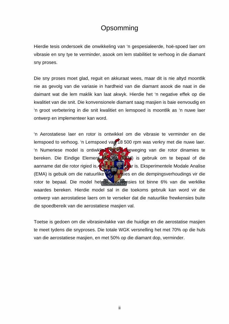
Each rough gem stone forms the basis for several finished products - the initial task
in the preparation involves studying the rough stone to decide on the most
profitable manner in which to pare it. The position for the initial cut is decided upon
by the marker and drawn in ink on the stone as a guide for the person responsible
for the paring. The paring is achieved by either cleaving or sawing – tasks on which
the quality of the finished stone is strongly dependant. These techniques are also
used to rough-cut each stone to the desired shape prior to polishing.
Mining of Rough Diamonds
Gem Diamonds Industrial Diamonds Boart
Industrial Use Gem Use
Studying & Marking of the Diamond
Cleaving Sawing Bruting
Polishing
Figure 1.1: Flow diagram illustrating the basic steps involved in diamond preparation.
1
The Design and Development of a High-speed Aerostatic Bearing
Diamond cleaving originating in India several centuries ago and was the first known
method of shaping a rough diamond. It thrived because it was the ideal method for
producing the octahedron shape, the basis for the point cut popular at the time. The
continued preference of round brilliants (a specific diamond cut) caused cleaving to
become almost obsolete, until a revival of the art in the 1970s due to the
introduction of the Princess cut (Watermeyer, 1982).
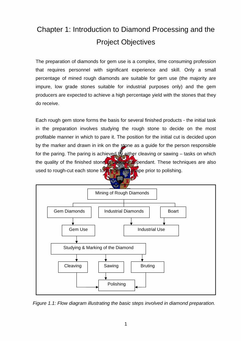
Cleaving involves splitting the stone using a blade and mallet. The stone is
cemented into a holder after which a groove, termed the kerf, is ground into the
marked lines of a single plane, normally using the sharp edge of a sawn off stone.
The blade is held in the kerf and tapped sharply using a steel rod or wooden mallet
with the intention of splitting the stone cleanly along the marked lines.
Figure 1.2: The implements used in diamond cleaving.
While sounding straightforward, cleaving is a practice requiring great precision and
its success relies heavily on the experience of the cleaver. Experienced cleavers
will admit that cleaving is never without risk as unknown variables such as
inclusions and internal stresses in the diamond make the outcome unpredictable.
The path of the fracture could easily deviate from the desired course, either
shattering the stone or at least resulting in a situation from which it is difficult to
salvage any good stones to work with. Cleaving is thus not as popular nowadays as
sawing which, while taking significantly longer (as much as a few days), is more
predictable, can be readily mechanized and does not rely as heavily on worker
experience (Watermeyer, 1982).
2
Chapter 1: Introduction to Diamond Processing and the Project Objectives
Bruting is a process similar to metal turning on a lathe, where a work stone (termed
the ‘sharp’) is used to shape the product stone. It is not an alternative method to
cleaving or sawing (as it is not a paring method as such) but is used for general
shaping before or after the paring process.
Diamond sawing originated from a method of separating diamonds using a fine wire
(of brass or iron) coated in oil and diamond powder (first documented in 1823). A
kerf is ground in the stone and the wire drawn repeatedly through it – teeth would
eventually form on the wire by the fine diamond particles which become embedded
in it. In this way the stone would be cut through, albeit very slowly with large stones
taking several months to separate. The first report of circular diamond sawing,
which uses a circular blade in a driven spindle, occurred in 1874, but due to the
steps taken to keep the method a secret, it was 40 years later that the practice
came into general use. Thus the method was never properly developed, and it is
only of late that it is reaching its full potential. Circular diamond sawing is now
considered a necessary task in diamond processing (Watermeyer, 1982).
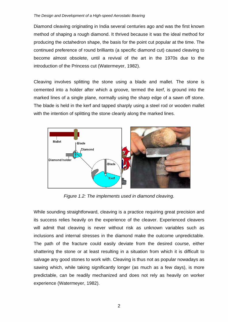
The rough stones come from the marker who has marked out the specific cut line.
The sawing needs to be completed accurately in terms of this line to maximise the
yield from the stone. There is only one opportunity for a successful cut and any
interruption to correct a deviation in the sawing line is rarely recoverable. This
requires that the process be smooth and exact – a task which is complicated by the
hardness of the diamond and the presence of unseen grains and imperfections
which deflect the blade and ruin the cut (Wilks and Wilks, 1994). For such an
important process, the sawing equipment currently available is very basic and does
not produce very reliable cuts.
Figure 1.3: The lines marked in black ink used to denote the desired sawing plane
(Lexus-com diamond equipment).
3
The Design and Development of a High-speed Aerostatic Bearing
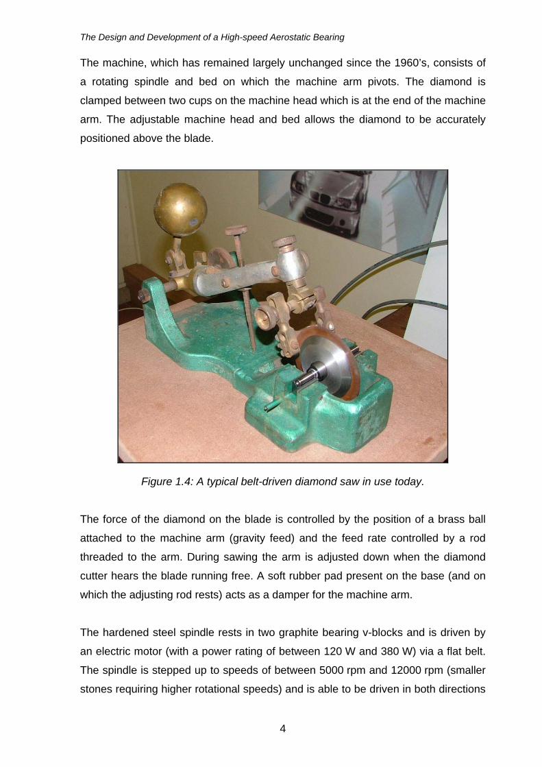
The machine, which has remained largely unchanged since the 1960’s, consists of
a rotating spindle and bed on which the machine arm pivots. The diamond is
clamped between two cups on the machine head which is at the end of the machine
arm. The adjustable machine head and bed allows the diamond to be accurately
positioned above the blade.
Figure 1.4: A typical belt-driven diamond saw in use today.
The force of the diamond on the blade is controlled by the position of a brass ball
attached to the machine arm (gravity feed) and the feed rate controlled by a rod
threaded to the arm. During sawing the arm is adjusted down when the diamond
cutter hears the blade running free. A soft rubber pad present on the base (and on
which the adjusting rod rests) acts as a damper for the machine arm.
The hardened steel spindle rests in two graphite bearing v-blocks and is driven by
an electric motor (with a power rating of between 120 W and 380 W) via a flat belt.
The spindle is stepped up to speeds of between 5000 rpm and 12000 rpm (smaller
stones requiring higher rotational speeds) and is able to be driven in both directions
4
Chapter 1: Introduction to Diamond Processing and the Project Objectives
via a reverse switch on the motor. The blocks and the belt tension control the radial
position of the spindle and suitable steps on the spindle itself control the axial
positioning.
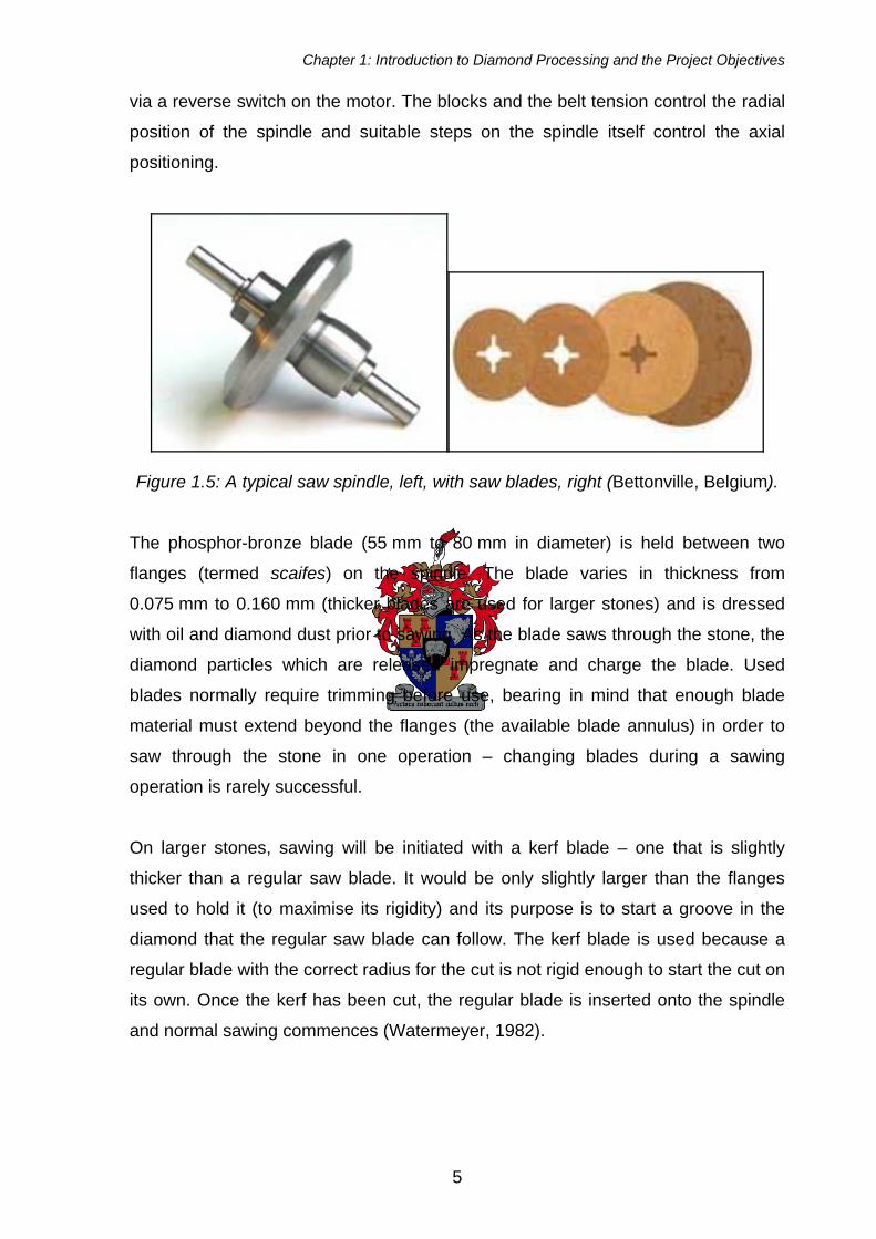
Figure 1.5: A typical saw spindle, left, with saw blades, right (Bettonville, Belgium).
The phosphor-bronze blade (55 mm to 80 mm in diameter) is held between two
flanges (termed scaifes) on the spindle. The blade varies in thickness from
0.075 mm to 0.160 mm (thicker blades are used for larger stones) and is dressed
with oil and diamond dust prior to sawing. As the blade saws through the stone, the
diamond particles which are released impregnate and charge the blade. Used
blades normally require trimming before use, bearing in mind that enough blade
material must extend beyond the flanges (the available blade annulus) in order to
saw through the stone in one operation – changing blades during a sawing
operation is rarely successful.
On larger stones, sawing will be initiated with a kerf blade – one that is slightly
thicker than a regular saw blade. It would be only slightly larger than the flanges
used to hold it (to maximise its rigidity) and its purpose is to start a groove in the
diamond that the regular saw blade can follow. The kerf blade is used because a
regular blade with the correct radius for the cut is not rigid enough to start the cut on
its own. Once the kerf has been cut, the regular blade is inserted onto the spindle
and normal sawing commences (Watermeyer, 1982).
5
The Design and Development of a High-speed Aerostatic Bearing
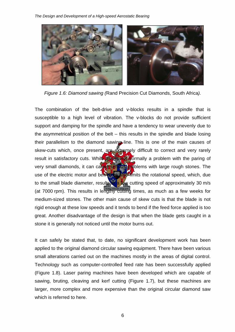
Figure 1.6: Diamond sawing (Rand Precision Cut Diamonds, South Africa).
The combination of the belt-drive and v-blocks results in a spindle that is
susceptible to a high level of vibration. The v-blocks do not provide sufficient
support and damping for the spindle and have a tendency to wear unevenly due to
the asymmetrical position of the belt – this results in the spindle and blade losing
their parallelism to the diamond sawing line. This is one of the main causes of
skew-cuts which, once present, are extremely difficult to correct and very rarely
result in satisfactory cuts. While this is not normally a problem with the paring of
very small diamonds, it can cause serious problems with large rough stones. The
use of the electric motor and belt drive also limits the rotational speed, which, due
to the small blade diameter, results in a low cutting speed of approximately 30 m/s
(at 7000 rpm). This results in lengthy cutting times, as much as a few weeks for
medium-sized stones. The other main cause of skew cuts is that the blade is not
rigid enough at these low speeds and it tends to bend if the feed force applied is too
great. Another disadvantage of the design is that when the blade gets caught in a
stone it is generally not noticed until the motor burns out.
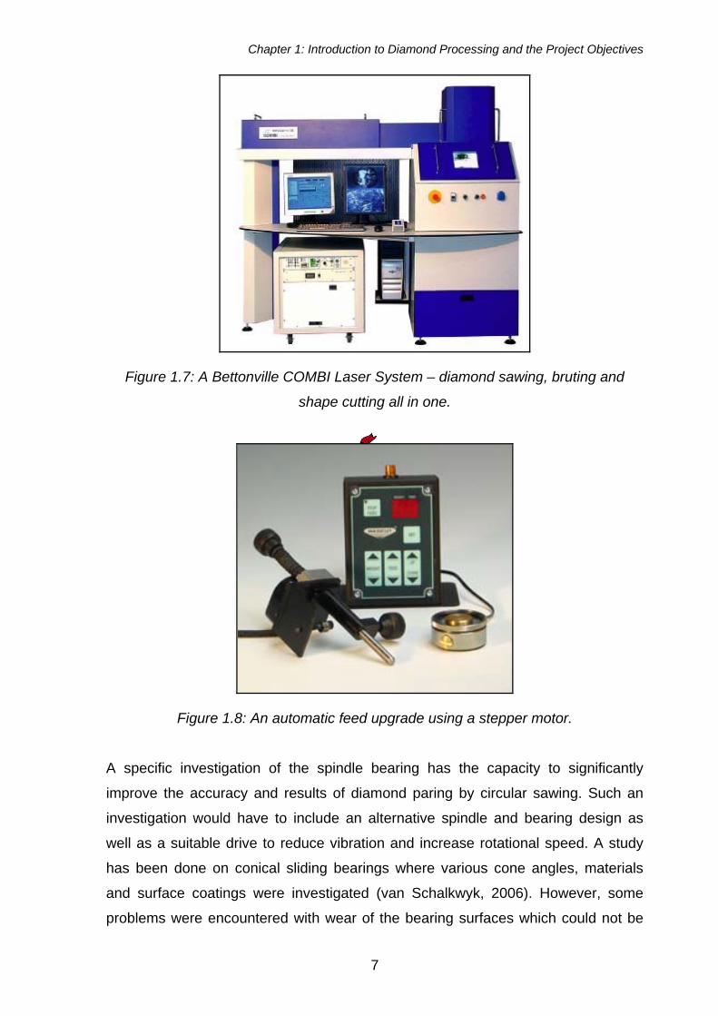
It can safely be stated that, to date, no significant development work has been
applied to the original diamond circular sawing equipment. There have been various
small alterations carried out on the machines mostly in the areas of digital control.
Technology such as computer-controlled feed rate has been successfully applied
(Figure 1.8). Laser paring machines have been developed which are capable of
sawing, bruting, cleaving and kerf cutting (Figure 1.7), but these machines are
larger, more complex and more expensive than the original circular diamond saw
which is referred to here.
6
Chapter 1: Introduction to Diamond Processing and the Project Objectives
Figure 1.7: A Bettonville COMBI Laser System – diamond sawing, bruting and
shape cutting all in one.
Figure 1.8: An automatic feed upgrade using a stepper motor.
A specific investigation of the spindle bearing has the capacity to significantly
improve the accuracy and results of diamond paring by circular sawing. Such an
investigation would have to include an alternative spindle and bearing design as
well as a suitable drive to reduce vibration and increase rotational speed. A study
has been done on conical sliding bearings where various cone angles, materials
and surface coatings were investigated (van Schalkwyk, 2006). However, some
problems were encountered with wear of the bearing surfaces which could not be
7
The Design and Development of a High-speed Aerostatic Bearing
resolved. Vibration levels tended to be too high and so it was decided that another
look at an alternative bearing design would be beneficial.
The aim of this project was to develop a superior, high-speed bearing to replace the
system used on conventional diamond sawing machines. Vibration levels and
cutting times were to be reduced in order to decrease cycle times and increase
production. In addition, a consistent and accurate blade position had to be ensured
to facilitate accurate sawing. A higher blade speed would also increase the rigidity
of the blade and help reduce the risk of skew cuts. The ultimate goal would be the
elimination of skew cuts, thus ensuring a higher production yield.
This report details the design and development of a high speed rotor supported by
an aerostatic bearing. Also included in the report are details of the modelling of the
rotor in order to accurately predict its dynamic characteristics at high speeds
(specifically natural modes and whirl magnitudes), so that stability of the sawing
operation can be assured. The modelling predominantly follows the principle of rigid
rotor dynamics, but a short investigation is done into flexible rotor analysis to
ascertain the validity of the rigid rotor assumption. The rotor is intended to be driven
by a mechanism of low vibration. The drive mechanism has been developed, but
the details are beyond the scope of this report.
The next chapter gives a brief review of previous research that is relevant to the
project. Chapter 3 details the development of the aerostatic bearing prototypes and
provides specifications for the two prototypes that were used for comparison
against the rotor models. The formulation of the finite element method (FEM) and
Euler rotor models is presented in Chapter 4, which also includes the results
obtained from these models. Chapter 5 presents the results obtained from
experimental modal analysis (EMA) of the two bearing systems, which are
compared with the model predictions. The conclusions and recommendations are
given in Chapter 6.
8
Chapter 2: Literature Survey
In this chapter, previous research relevant to the project is reviewed. Previous
relevant research can be divided into two areas: aerostatic bearing design and the
dynamic analysis of rotating shafts (rotordynamics). A large amount of attention has
been given to both of these areas as separate fields of study. However, the amount
of literature concerning the rotordynamics of aerostatic journal bearings is limited.
This in itself is not a problem as the principles of rotordynamics can readily be
applied to the case of aerostatic bearings. Most of the research available focuses
on either flexible shafts with a concentrated mass between two supports or the whirl
of rigid shafts supported by hydrodynamic bearings (Surial and Kaushal, undated;
Abulrub et al. 2005; Nicholas et al. undated; Antkowiak and Nelson, 1997). What
makes this study distinct is that, contrary to hydrodynamic bearing research, it does
not consider fluid dynamics in any detail – it is a rotordynamic study applied to
aerostatic bearings. The rotor is modelled with a non-symmetric centre of gravity
(CG) and is supported by a single, central bearing area with a non-constant
stiffness distribution along its length. This makes it different to the research
concerned with two or more concentrated bearing supports of specific stiffness.
2.1. Recent research in bearing concepts for the diamond saw
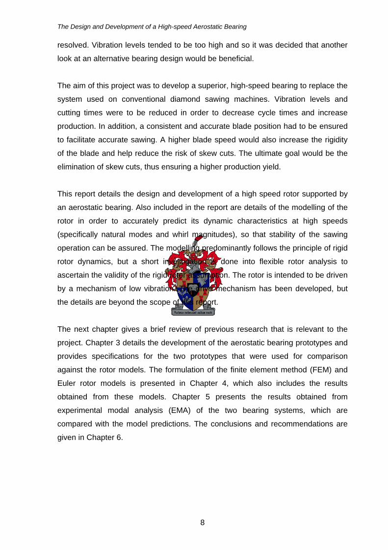
In order to address the requirement for reduced vibration, a new bearing concept
for the diamond saw was the main focus in the early stages of the project, done by
van Schalkwyk (2006). The initial concept was a spindle with conical ends which
rotated within female bushes. This type of dry, sliding bearing was similar to the
graphite bearings of the conventional saw and if successful would be a simple
modification. Various tests were conducted with the aim of determining the most
appropriate material combination of the spindle and bushes.
A tool-steel spindle with a chemical vapour deposition (CVD) coating, running in
similarly coated carbide bushes tended to wear heavily after approximately 10
hours of operation, with the majority of the wear occurring on the rotor and not on
the bushes which would have been preferred. An improved spindle with detachable
conical ends allowed a harder thermal diffusion (TD) coating to be used.
9
The Design and Development of a High-speed Aerostatic Bearing
Figure 2.1: The sliding bearing design by van Schalkwyk (2006).
When run in graphite bushes no visible wear on the spindle occurred, however the
graphite was too soft and brittle to be considered for the application. Ceramic
bushes were more successful in terms of strength, but particles tended to break
away from the bushes, wearing the coated spindle heavily (van Schalkwyk, 2006).
2.2. Recent research in gas film bearings
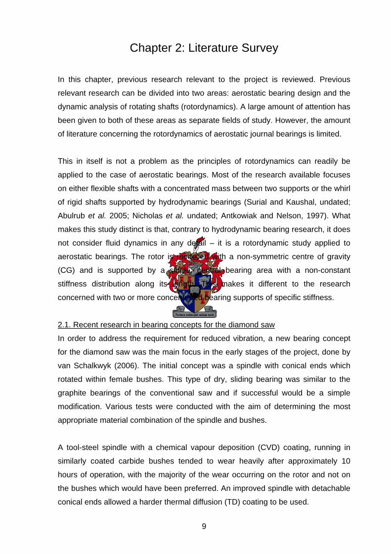
Much research has been done in recent years on gas film bearings for modern-
technology applications. Focus has specifically been given to micro-
electromechanical systems (MEMS), micro-scale machines (compressors, turbines
etc.) for propulsion and mobile power generation etc (Piers et al. 2003). These
micro-machines must rotate at very high speeds (on the order of 1x10⁶ rpm) in
order to achieve power densities comparable with normal-scale turbomachines, and
thus low friction bearings are required. Current limitations in microfabrication
techniques result in low length-to-diameter (aspect) ratios (0.1:1) compared to
typical gas-film bearings in industrial applications (1:1 to 4:1). The clearance ratios
are also much larger than typical gas film bearings. Figure 2.2 shows a typical
micro-motor - the thin outer rim of the bearing provides radial support with thrust
bearings at each end. One face would typically house either a motor or a generator.
10
Chapter 2: Literature Survey
Figure 2.2: A cross-sectional view through a typical micro-rotor.
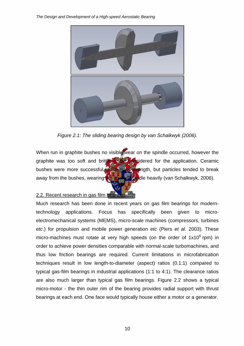
Wong et al. (2002) developed a self-acting (aerodynamic) bearing of 4.2 mm
diameter for a high speed micro-rotor. It was successfully rotated at 450 000 rpm,
driven by a micro-scale radial inflow turbine. It was suggested that without the
design constraints present, more than 1x10⁶ rpm would be possible. The
aerodynamic principle was researched to eliminate two disadvantages present with
an aerostatic bearing – the air supply requirement and the increased manufacturing
complexity of using feed orifices in micro-machines.
Figure 2.3: A comparison of theoretical and experimental load capacities for an
aerodynamic micro-bearing (Wong, 2002).
11
The Design and Development of a High-speed Aerostatic Bearing
Equations for load carrying capacity and drag (which are dependent on rotor speed)
were derived. A full profile spiral groove was incorporated into the thrust face to
maximise load capacity and bearing stiffness. The stiffness was proportional to the
rotor speed and reached 6x10⁵ N/m at 820 000 rpm (constant 3x10⁵ N/m for the
aerostatic bearing). It was shown that at speeds below 100 000 rpm the
aerodynamic load capacity was less than that required to support the aft rotor
forces (aerostatic support was used to carry the rotor above this speed). At speeds
exceeding 169 0000 rpm the aerodynamic capacity alone was sufficient. The gross
load carrying capacity of the bearing was approximately 50% greater than predicted
by the theory, but followed the same trend with increasing speed.
A second-order, two degree of freedom (DOF) model was developed by Savoulides
et al. (2000) to analyse the stability region and whirling frequency of a balanced
micro-scale gas bearing. This model development was prompted by the inability of
conventional theory and design tools to adequately model these unique bearings.
For increased stability, high and low pressure plenums were used to impart a net
load on the rotor thereby displacing it radially from the bearing’s geometric centre.
Thus the eccentricity of the rotor could be controlled during testing. Stiffness
coefficients consisted of hydrodynamic stiffness (derived from numerical simulation
of the Reynolds equation) and hydrostatic stiffness (derived from a numerical model
for axial flow through a short bearing, developed by Piekos). Damping coefficients
were derived from the Full-Sommerfield short-width bearing theory. The stability
boundary (defined by a load parameter) plotted by the model against the bearing
number showed good agreement with the compressible Reynolds equation. While
the model results are slightly lower than the full numerical simulation, they are
obtained much quicker, and illustrate the same trend. In conclusion, it was noted
that aerostatic support was beneficial at low speeds (making start-up at the high
eccentricities possible) with a transition to aerodynamic support at higher speeds.
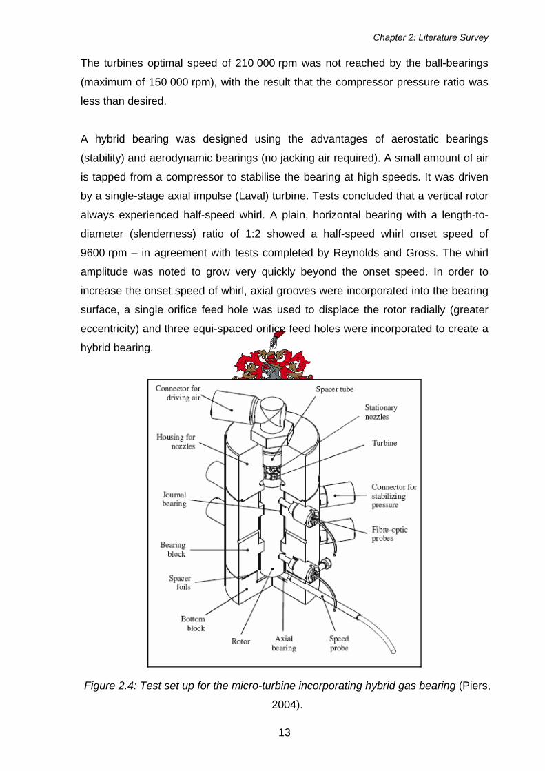
Piers et al. (2004) developed a hybrid gas bearing to replace the high-speed ball-
bearings in a micro-gas turbine (Figure 2.4). A maximum rotational speed of
96 000 rpm was attained with the gas bearing. In order to maximise the efficiency
and output of these micro-turbines the rotational speed has to be extremely high.
12
Chapter 2: Literature Survey
The turbines optimal speed of 210 000 rpm was not reached by the ball-bearings
(maximum of 150 000 rpm), with the result that the compressor pressure ratio was
less than desired.
A hybrid bearing was designed using the advantages of aerostatic bearings
(stability) and aerodynamic bearings (no jacking air required). A small amount of air
is tapped from a compressor to stabilise the bearing at high speeds. It was driven
by a single-stage axial impulse (Laval) turbine. Tests concluded that a vertical rotor
always experienced half-speed whirl. A plain, horizontal bearing with a length-to-
diameter (slenderness) ratio of 1:2 showed a half-speed whirl onset speed of
9600 rpm – in agreement with tests completed by Reynolds and Gross. The whirl
amplitude was noted to grow very quickly beyond the onset speed. In order to
increase the onset speed of whirl, axial grooves were incorporated into the bearing
surface, a single orifice feed hole was used to displace the rotor radially (greater
eccentricity) and three equi-spaced orifice feed holes were incorporated to create a
hybrid bearing.
Figure 2.4: Test set up for the micro-turbine incorporating hybrid gas bearing (Piers,
2004).
13
The Design and Development of a High-speed Aerostatic Bearing
The axially grooved bearing was limited to 26 000 rpm (horizontally) and
18 000 rpm (vertically). It was noted that the 26 000 rpm limit on the horizontal rotor
was due to fractional-speed whirl. Starting the rotor with a single orifice feed was
difficult and no reliable conclusions could be drawn. The hybrid bearing was able to
reach 96 000 rpm before limited by fractional whirl.
J.P. Khatait et al. (2005) investigated the effect of orifice diameter, clearance,
supply pressure and bearing diameter on the load capacity and stiffness of an
aerostatic thrust bearing with the aim of using simple tools to build low cost, high
performance air bearings. In addition, a computational fluid dynamics (CFD)
analysis was done to plot the pressure distribution radially along the bearing
surface. This also agreed well with the theory, except for a pressure drop at the
pocket edge, which was attributed to throttling. Experimental testing showed good
agreement with his analysis at large clearances, with some deviation occurring at
smaller clearances.
2.3. Recent research in high-speed rotordynamics
In the past decade, new methods to increase rotational speeds and improve
stability and control of rotating machinery have remained key focus areas for
manufacturing, power production and aerospace industries. This has resulted in
ongoing research focusing specifically in areas of high-speed rotordynamics.
G.V. Brown et al. (2006) developed a superior control system for magnetic bearings
which support high-speed flywheels. The specific aim of the research was to
stabilize the forward and backward tilt whirling modes, the frequencies of which
depend on the shaft speed due to gyroscopic effects. These modes are normally
instable and exhibit low damping and thus often prevent the attainment of the
desired shaft speed.
A rigid shaft was considered, treated as a free body and acted upon only by the
speed dependent gyroscopic torques and the support forces from the two magnetic
bearings. Only the tilt modes were considered – all of the pure translation modes
were ignored. It was noted that the product of the absolute values of the
frequencies was approximately constant with rotor speed and that the damping
14
Chapter 2: Literature Survey
ratios of the two modes were identical. However, the damping coefficient of the
forward-whirl mode is greater than the backward-whirl mode due to the fact that the
mode occurs at a higher frequency.
Cross-axis proportional gains are investigated as a superior alternative to same-
axis derivative or cross-axis derivative gains in magnetic bearing control systems.
Due to the tilt mode’s dependency on rotor speed it is possible to completely
eliminate the need for differentiation of the displacement to obtain shaft velocity.
However the cross-axis proportional gain required to stabilise the forward-whirl
mode destabilizes the backward-whirl mode and vice-versa. This was overcome by
taking advantage of the increased difference in the frequencies of the two modes
that occurs at high rotor speeds. Two parallel paths are utilized in the controller
separated by high- and low-pass filters. The path using the low-pass filter stabilizes
the backward-whirl mode using an appropriate signed cross-axis proportional gain,
and other using the high-pass filter stabilizes the forward-whirl mode with an
oppositely-signed cross-axis proportional gain.
The effectiveness of using cross-axis proportional gains was investigated in an
energy storage flywheel at speeds of up to 60 000 rpm. An unfiltered cross-axis
gain could only reduce the amplitude of one of the whirl modes at a time. A filtered
cross-axis gain was effective in reduce the amplitude of both whirl modes
simultaneously.
The research of M.I. Friswell et al. (2000) focused on how gyroscopic forces and
bearing characteristics cause bifurcation of the natural frequencies and damping
ratios of the tilt modes as the shaft rotational speed is increased. Two cases for
rigid rotors were considered: one for when the bearing supports are isotropic in
terms of stiffness and damping and the other where the supports display isotropic
stiffness but anisotropic damping.
A theoretical derivation for the first case (isotropic damping) showed that the natural
frequencies will separate but the damping ratio will stay the same for the two
modes. Above a certain speed the same trend is displayed for the second case
(anisotropic damping), but the behaviour is dependent on the mean of the damping
15
The Design and Development of a High-speed Aerostatic Bearing
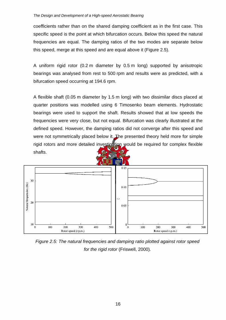
coefficients rather than on the shared damping coefficient as in the first case. This
specific speed is the point at which bifurcation occurs. Below this speed the natural
frequencies are equal. The damping ratios of the two modes are separate below
this speed, merge at this speed and are equal above it (Figure 2.5).
A uniform rigid rotor (0.2 m diameter by 0.5 m long) supported by anisotropic
bearings was analysed from rest to 500 rpm and results were as predicted, with a
bifurcation speed occurring at 194.6 rpm.
A flexible shaft (0.05 m diameter by 1.5 m long) with two dissimilar discs placed at
quarter positions was modelled using 6 Timosenko beam elements. Hydrostatic
bearings were used to support the shaft. Results showed that at low speeds the
frequencies were very close, but not equal. Bifurcation was clearly illustrated at the
defined speed. However, the damping ratios did not converge after this speed and
were not symmetrically placed below it. The presented theory held more for simple
rigid rotors and more detailed investigation would be required for complex flexible
shafts.
Figure 2.5: The natural frequencies and damping ratio plotted against rotor speed
for the rigid rotor (Friswell, 2000).
16
Chapter 3: The Design of the Rotor and Aerostatic Bearing
This chapter concerns the design of the rotor and the aerostatic bearing in which it
would run. It includes customer requirements and specifications for the diamond
saw, general information on the bearing design as well as individual component
specifications. A design strategy for the aerostatic bearing is also included.
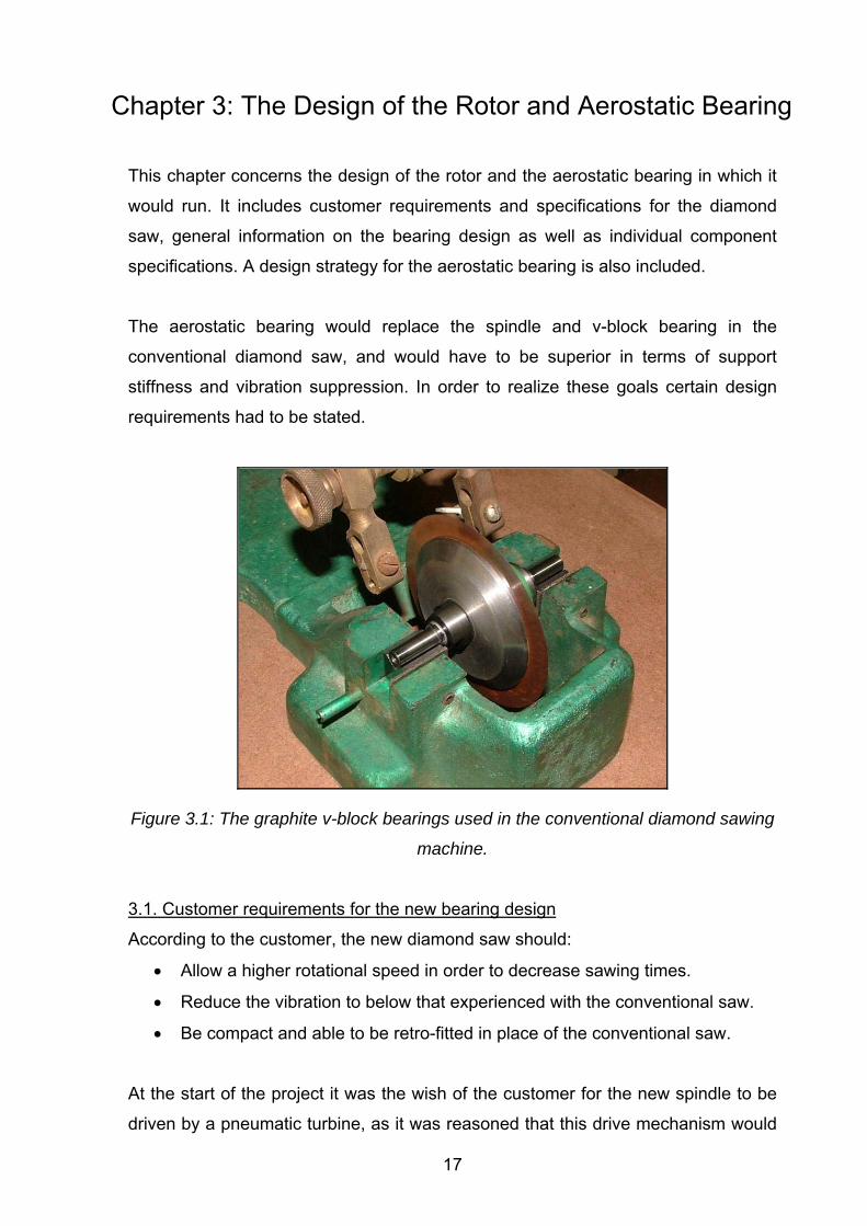
The aerostatic bearing would replace the spindle and v-block bearing in the
conventional diamond saw, and would have to be superior in terms of support
stiffness and vibration suppression. In order to realize these goals certain design
requirements had to be stated.
Figure 3.1: The graphite v-block bearings used in the conventional diamond sawing
machine.
3.1. Customer requirements for the new bearing design
According to the customer, the new diamond saw should:
• Allow a higher rotational speed in order to decrease sawing times.
• Reduce the vibration to below that experienced with the conventional saw.
• Be compact and able to be retro-fitted in place of the conventional saw.
At the start of the project it was the wish of the customer for the new spindle to be
driven by a pneumatic turbine, as it was reasoned that this drive mechanism would
17
The Design and Development of a High-speed Aerostatic Bearing
combine high speeds with the lowest vibration transmission. Thus, additional
customer requirements were specified for the turbine:
• The rotor should be driven in both directions by a pneumatic turbine.
• The turbine should operate off a common workshop air supply.
• The turbine should be efficient in terms of power consumption.
3.2. Engineering requirements for the new bearing design
The following engineering requirements were specified for the new saw:
• The operating speed should be increased to 20 000 rpm. The lowest natural
frequency of the system should be 20% higher than the highest operational
speed (i.e. greater than 24 000 rpm, 400 Hz).
• The RMS acceleration value in the range 0 - 2 kHz measured on the bearing
housing at 20 000 rpm should be less 0.04 m/s2.
• The bearing lifetime should be no less than five years (maintenance free)
and as long as practically possible.
• The minimum power output of the rotor drive should be 500 W at 25 000 rpm.
• The radial load capacity of the bearing should be at least 20 N.
• The bearing should operate off a 5 bar workshop air supply.
• The turbine, if used, should be small enough in size and weight not to
dominate the rotor’s dynamic characteristics.
• The coupling of the rotor to the drive should be of such a design that no ill-
effect is suffered in the case of the blade catching in the stone.
• The entire saw should fit in the space occupied by the existing spindle and
able to be retro-fitted in place of it.
• The total air consumption of the saw should be less than 200 l/min.
Concerning the drive, a simple radial air-turbine was investigated utilizing the same
air source as the bearing. In addition a high speed brushless DC motor was also
considered. Values of the cutting force during sawing were not available making it
difficult to accurately predict the power requirement for successful sawing at
20 000 rpm. The power requirement of 500 W has been calculated from the fact
that 120 W machines are conventionally being used to saw stones at 7000 rpm.
However, the design and selection of the drive mechanism is beyond the scope of
this report.
18
Chapter 3: The Design of the Rotor and Aerostatic Bearing
3.3. Bearing concepts – reasons for the use of an aerostatic bearing
The bearing concepts considered for the new sawing machine were sliding
bearings, rolling contact bearings (ball or roller), magnetic bearings, liquid lubricated
bearings and gas lubricated bearings. The first of these bearing types were
eliminated as possibilities for various reasons, leaving the gas lubricated bearing as
the most capable concept for the application.
As mentioned in the literature survey (Chapter 2), conical sliding bearings were
investigated and eliminated on the following grounds:
• Friction and subsequent heat build-up limited high speed operation.
• Vibration levels were too high.
• A lack of suitable bearing materials.
Rolling contact bearings would have been limited in the speed requirement of the
new saw. Special roller bearings rated at 25 000 rpm are available, but require
cooling and would have a limited lifespan. A gas lubricated bearing would be able to
run at the desired operating speed without any cooling system required, and the
vibration transmitted would be lower than with roller contact bearings. In addition
the gas bearing would have lower friction, allowing for a less powerful drive and a
longer bearing life. Roller contact bearings would also make axle removal (in the
case of blade changing) impossible if the original design layout was retained.
Magnetic bearings would have been another promising bearing type to consider in
terms of vibration and friction, but were eliminated due to the complexity of the
control system required and the added risk on ensuring a constant power source.
Similarly, liquid bearings could have been successfully implemented but would have
required a cooling system, a pumping system and a storage volume, none of which
is required for an aerostatic type. The larger load capacity of the liquid bearing
would not be required in the diamond saw application, and the friction would be
larger than that of a gas bearing.
Of the gas lubricated bearing types, an aerostatic bearing was considered superior
to an aerodynamic type in terms of load capacity, stability, ease of manufacture and
19
The Design and Development of a High-speed Aerostatic Bearing
surface wear. It was therefore chosen as the bearing type to be used in the new
diamond saw, and would provide the following advantages:
• Low levels of friction allowing for low vibration and high speeds without
cooling. Low vibration transmission and moderate damping properties of the
air film would allow for a lighter rotor housing and base.
• Only an additional small compressor would be required; no cooling systems
or gas storage volume tanks would be necessary.
• The load capacity of a medium sized aerostatic bearing would be sufficient in
the low-load application of the diamond saw.
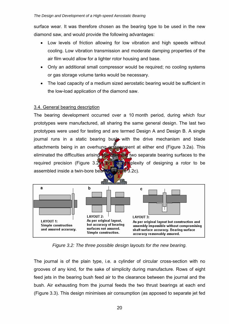
3.4. General bearing description
The bearing development occurred over a 10 month period, during which four
prototypes were manufactured, all sharing the same general design. The last two
prototypes were used for testing and are termed Design A and Design B. A single
journal runs in a static bearing bush with the drive mechanism and blade
attachments being in an overhung arrangement at either end (Figure 3.2a). This
eliminated the difficulties arising from aligning two separate bearing surfaces to the
required precision (Figure 3.2b) or the complexity of designing a rotor to be
assembled inside a twin-bore bearing (Figure 3.2c).
Figure 3.2: The three possible design layouts for the new bearing.
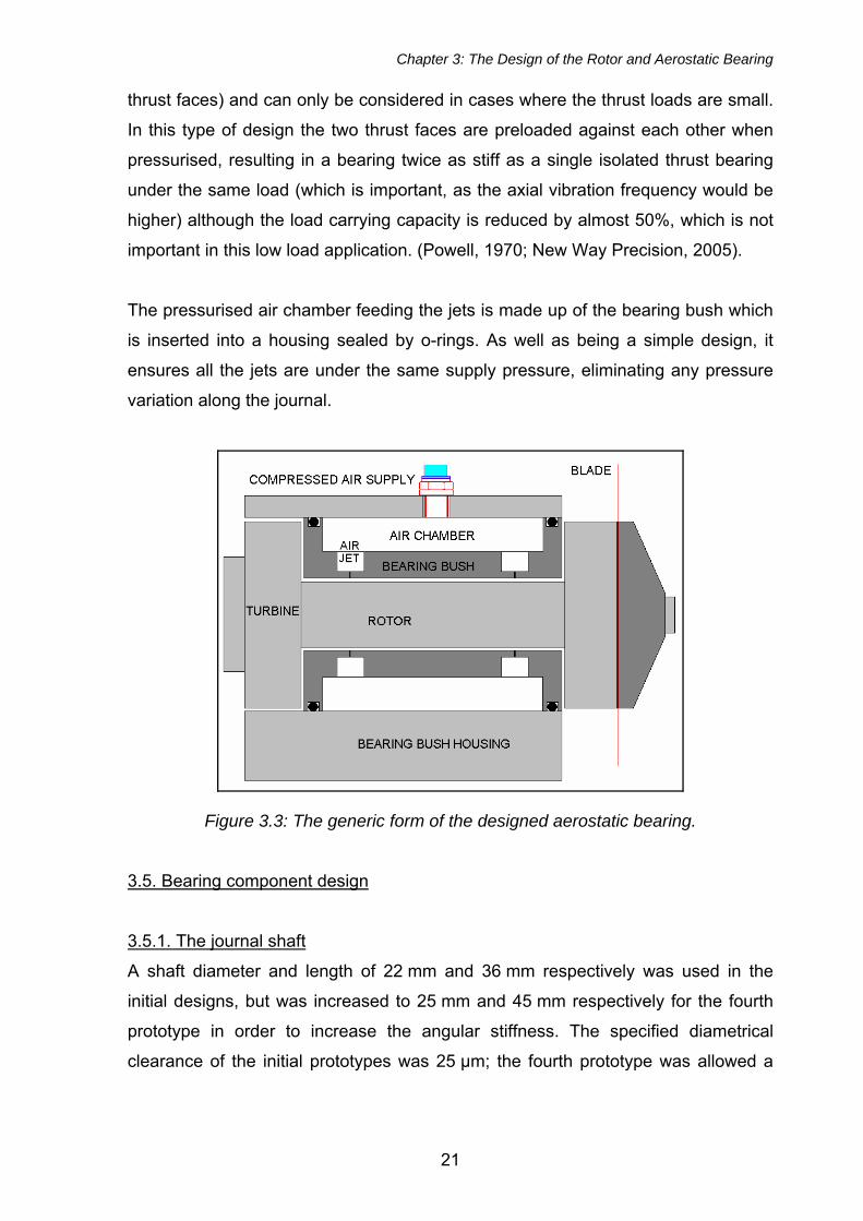
The journal is of the plain type, i.e. a cylinder of circular cross-section with no
grooves of any kind, for the sake of simplicity during manufacture. Rows of eight
feed jets in the bearing bush feed air to the clearance between the journal and the
bush. Air exhausting from the journal feeds the two thrust bearings at each end
(Figure 3.3). This design minimises air consumption (as apposed to separate jet fed
20
Chapter 3: The Design of the Rotor and Aerostatic Bearing
thrust faces) and can only be considered in cases where the thrust loads are small.
In this type of design the two thrust faces are preloaded against each other when
pressurised, resulting in a bearing twice as stiff as a single isolated thrust bearing
under the same load (which is important, as the axial vibration frequency would be
higher) although the load carrying capacity is reduced by almost 50%, which is not
important in this low load application. (Powell, 1970; New Way Precision, 2005).
The pressurised air chamber feeding the jets is made up of the bearing bush which
is inserted into a housing sealed by o-rings. As well as being a simple design, it
ensures all the jets are under the same supply pressure, eliminating any pressure
variation along the journal.
Figure 3.3: The generic form of the designed aerostatic bearing.
3.5. Bearing component design
3.5.1. The journal shaft
A shaft diameter and length of 22 mm and 36 mm respectively was used in the
initial designs, but was increased to 25 mm and 45 mm respectively for the fourth
prototype in order to increase the angular stiffness. The specified diametrical
clearance of the initial prototypes was 25 μm; the fourth prototype was allowed a
21
The Design and Development of a High-speed Aerostatic Bearing
diametrical clearance of 36 μm to ease manufacture. These clearances are
considered medium to large by aerostatic bearing standards.
It is generally recommended that the tolerance on the shaft diameter be no more
than one-third of that of the mean radial clearance (MRC). As the MRC was
12.5 μm (18 μm for the fourth prototype), the shaft diameter was limited to a 5 μm
tolerance along its length (6 μm for the fourth prototype). This tolerance is not small
by aerostatic component standards, but was considered very tight by the
machinists. The MRC was thus a compromise between the reliable accuracy of the
machinists and the air consumption of the bearing, which is normally required to be
an absolute minimum, bearing in mind that the air consumption increased with the
cubed power of the MRC. This applies to the bearing bush machining as well.
Shaft material was initially hard-anodised aluminium (chosen to reduce rotor mass),
which was inadequate in the event of rotor contact. The shafts have to be ground to
size, which is only possible on an aluminium component if it is hard-anodised. It
would mark easily and anodised particles would come free, blocking the clearance
and making it necessary to disassemble and clean the bearing.
Taking into account the fact that a high polar moment of inertia for the rotor was as
an important criteria as low mass, a high-carbon, high-chromium tool steel (Bohler
K110) was specified for the fourth prototype. This provided the necessary surface
finish after grinding and could also be finished to the required tolerance more
reliably than the anodized aluminium. The increased eccentric position of the
heavier rotor would theoretically result in greater stability due to higher damping
(which increases with the eccentricity ratio). Also, small imbalance inducing events
(blade damage etc) would have less of an effect on the overall balance of the rotor
if it were heavier. However the steel also tended to mark in the event of rotor
contact, though not as badly as with the hard-anodised aluminium.
Regarding material choice and the rotor’s natural frequencies, a compromise has to
be made against the mass and polar moment of inertia of the rotor. The highest
inertia possible is desired while still ensuring that the lowest natural mode is higher
than 400 Hz. As stainless-steel was used for the bearing bush, it was never
considered as a shaft material in view of its tendency to seize when run together.
22
Chapter 3: The Design of the Rotor and Aerostatic Bearing
Shaft surface material selection was never considered more important than
eliminating the risk of rotor contact itself (which should not occur until the most
arduous conditions are reached). However, material selection is important from the
point of view that should contact occur (due to a broken blade, inferior balancing or
insufficient bearing pressure) it should be a minor event limited to investigation into
the cause and not requiring extensive repairs.
3.5.2. The bearing bush
The journal shaft rotates within the bearing bush which houses the air feed jets.
Both aluminium and stainless steel were used as materials, with the stainless steel
being preferable for the following reasons:
• The aluminium bush could only be turned to size (anodising was not an
option in the bore) whereas the stainless-steel could be ground and/or honed
to size. This improved the ability to ensure the correct shaft tolerance.
• The surface finish obtained on the stainless bush was slightly better than
with the aluminium.
• The stainless-steel was more wear resistant than the aluminium.
• With the use of simple jets (discussed in Section 3.5.3), the stainless-steel
bush would be less prone to distortion when the jets are inserted – this is
very important considering the small clearances involved.
The two flat faces of the bush form part of the axial thrust bearings and are thus
finished as per the journal shaft, with special attention given to ensure that they are
perpendicular to the bore axis. Each end of the bush makes provision for an o-ring
to seal the air cavity that is created when the bush is inserted into the housing.
3.5.3. The feed jets
Two jet positions were investigated – half-station and quarter-station. This refers to
the position of the jet relative to each end of the journal. A half-station bearing has a
single row of jets halfway along the journal length. A quarter-station bearing has two
rows of jets positioned one-quarter of the journal length from each end; this
improves bearing stiffness at the expense of air consumption, which is effectively
doubled (Figure 3.4).
23
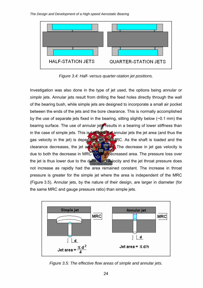
The Design and Development of a High-speed Aerostatic Bearing
Figure 3.4: Half- versus quarter-station jet positions.
Investigation was also done in the type of jet used, the options being annular or
simple jets. Annular jets result from drilling the feed holes directly through the wall
of the bearing bush, while simple jets are designed to incorporate a small air pocket
between the ends of the jets and the bore clearance. This is normally accomplished
by the use of separate jets fixed in the bearing, sitting slightly below (~0.1 mm) the
bearing surface. The use of annular jets results in a bearing of lower stiffness than
in the case of simple jets. This is because for annular jets the jet area (and thus the
gas velocity in the jet) is dependent on the MRC. As the shaft is loaded and the
clearance decreases, the jet area decreases. The decrease in jet gas velocity is
due to both the decrease in MRC and the decreased area. The pressure loss over
the jet is thus lower due to the decreased velocity and the jet throat pressure does
not increase as rapidly had the area remained constant. The increase in throat
pressure is greater for the simple jet where the area is independent of the MRC
(Figure 3.5). Annular jets, by the nature of their design, are larger in diameter (for
the same MRC and gauge pressure ratio) than simple jets.
Figure 3.5: The effective flow areas of simple and annular jets.
24
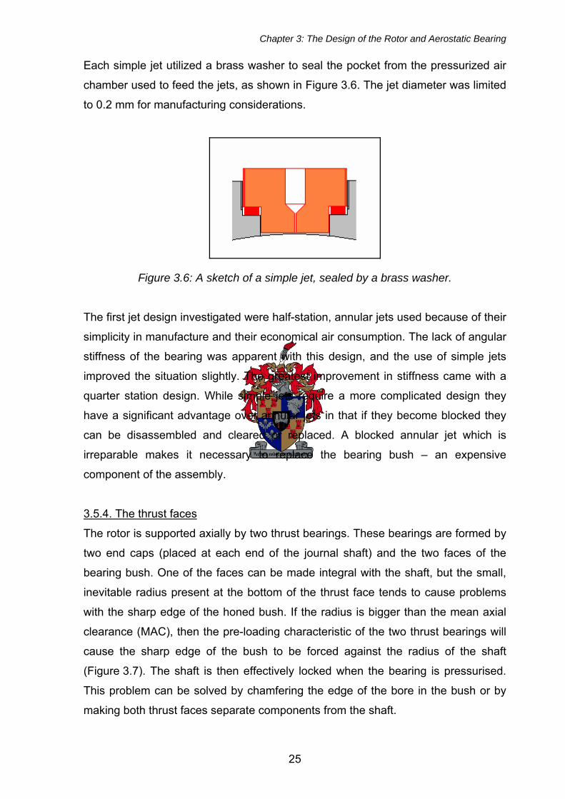
Chapter 3: The Design of the Rotor and Aerostatic Bearing
Each simple jet utilized a brass washer to seal the pocket from the pressurized air
chamber used to feed the jets, as shown in Figure 3.6. The jet diameter was limited
to 0.2 mm for manufacturing considerations.
Figure 3.6: A sketch of a simple jet, sealed by a brass washer.
The first jet design investigated were half-station, annular jets used because of their
simplicity in manufacture and their economical air consumption. The lack of angular
stiffness of the bearing was apparent with this design, and the use of simple jets
improved the situation slightly. The greatest improvement in stiffness came with a
quarter station design. While simple jets require a more complicated design they
have a significant advantage over annular jets in that if they become blocked they
can be disassembled and cleared or replaced. A blocked annular jet which is
irreparable makes it necessary to replace the bearing bush – an expensive
component of the assembly.
3.5.4. The thrust faces
The rotor is supported axially by two thrust bearings. These bearings are formed by
two end caps (placed at each end of the journal shaft) and the two faces of the
bearing bush. One of the faces can be made integral with the shaft, but the small,
inevitable radius present at the bottom of the thrust face tends to cause problems
with the sharp edge of the honed bush. If the radius is bigger than the mean axial
clearance (MAC), then the pre-loading characteristic of the two thrust bearings will
cause the sharp edge of the bush to be forced against the radius of the shaft
(Figure 3.7). The shaft is then effectively locked when the bearing is pressurised.
This problem can be solved by chamfering the edge of the bore in the bush or by
making both thrust faces separate components from the shaft.
25
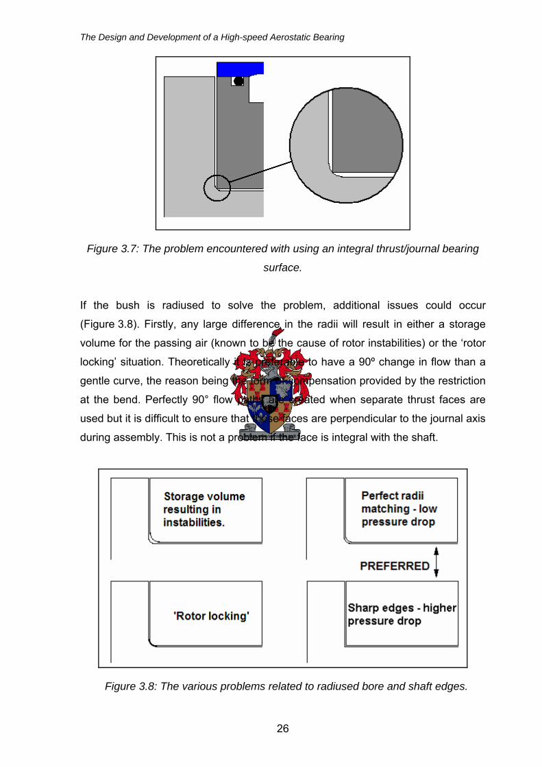
The Design and Development of a High-speed Aerostatic Bearing
Figure 3.7: The problem encountered with using an integral thrust/journal bearing
surface.
If the bush is radiused to solve the problem, additional issues could occur
(Figure 3.8). Firstly, any large difference in the radii will result in either a storage
volume for the passing air (known to be the cause of rotor instabilities) or the ‘rotor
locking’ situation. Theoretically it is preferable to have a 90º change in flow than a
gentle curve, the reason being the form of compensation provided by the restriction
at the bend. Perfectly 90° flow paths are created when separate thrust faces are
used but it is difficult to ensure that these faces are perpendicular to the journal axis
during assembly. This is not a problem if the face is integral with the shaft.
Figure 3.8: The various problems related to radiused bore and shaft edges.
26
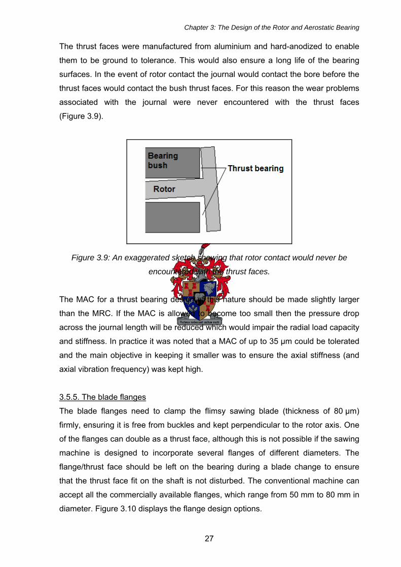
Chapter 3: The Design of the Rotor and Aerostatic Bearing
The thrust faces were manufactured from aluminium and hard-anodized to enable
them to be ground to tolerance. This would also ensure a long life of the bearing
surfaces. In the event of rotor contact the journal would contact the bore before the
thrust faces would contact the bush thrust faces. For this reason the wear problems
associated with the journal were never encountered with the thrust faces
(Figure 3.9).
Figure 3.9: An exaggerated sketch showing that rotor contact would never be
encountered with the thrust faces.
The MAC for a thrust bearing design of this nature should be made slightly larger
than the MRC. If the MAC is allowed to become too small then the pressure drop
across the journal length will be reduced which would impair the radial load capacity
and stiffness. In practice it was noted that a MAC of up to 35 μm could be tolerated
and the main objective in keeping it smaller was to ensure the axial stiffness (and
axial vibration frequency) was kept high.
3.5.5. The blade flanges
The blade flanges need to clamp the flimsy sawing blade (thickness of 80 µm)
firmly, ensuring it is free from buckles and kept perpendicular to the rotor axis. One
of the flanges can double as a thrust face, although this is not possible if the sawing
machine is designed to incorporate several flanges of different diameters. The
flange/thrust face should be left on the bearing during a blade change to ensure
that the thrust face fit on the shaft is not disturbed. The conventional machine can
accept all the commercially available flanges, which range from 50 mm to 80 mm in
diameter. Figure 3.10 displays the flange design options.
27
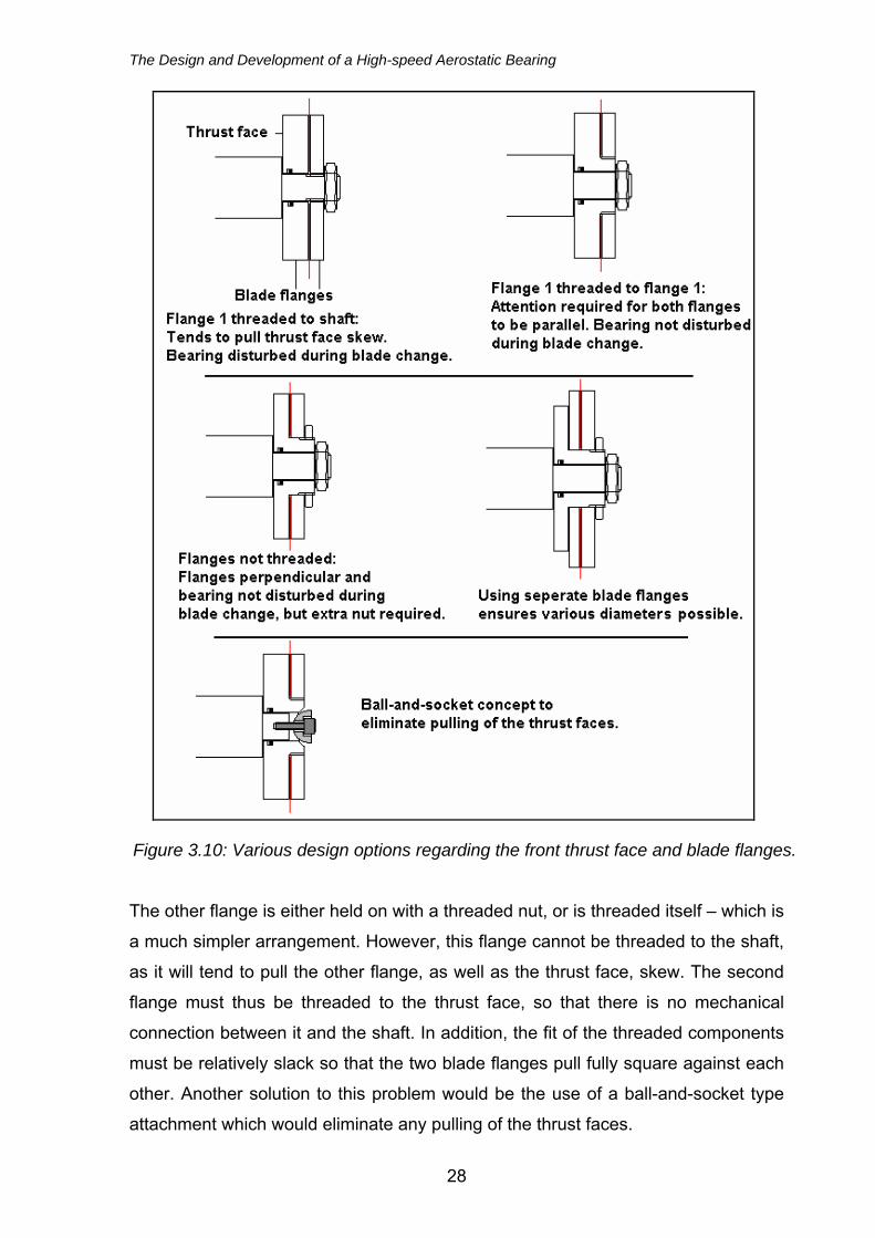
The Design and Development of a High-speed Aerostatic Bearing
Figure 3.10: Various design options regarding the front thrust face and blade flanges.
The other flange is either held on with a threaded nut, or is threaded itself – which is
a much simpler arrangement. However, this flange cannot be threaded to the shaft,
as it will tend to pull the other flange, as well as the thrust face, skew. The second
flange must thus be threaded to the thrust face, so that there is no mechanical
connection between it and the shaft. In addition, the fit of the threaded components
must be relatively slack so that the two blade flanges pull fully square against each
other. Another solution to this problem would be the use of a ball-and-socket type
attachment which would eliminate any pulling of the thrust faces.
28
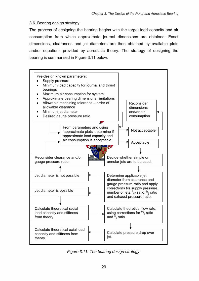
Chapter 3: The Design of the Rotor and Aerostatic Bearing
3.6. Bearing design strategy
The process of designing the bearing begins with the target load capacity and air
consumption from which approximate journal dimensions are obtained. Exact
dimensions, clearances and jet diameters are then obtained by available plots
and/or equations provided by aerostatic theory. The strategy of designing the
bearing is summarised in Figure 3.11 below.
Pre-design known parameters: • Supply pressure • Minimum load capacity for journal and thrust
bearings • Maximum air consumption for system • Approximate bearing dimensions, limitations • Allowable machining tolerance – order of
allowable clearance • Minimum jet diameter • Desired gauge pressure ratio
From parameters and using ‘approximate plots’ determine if approximate load capacity and air consumption is acceptable.
Not acceptable
Reconsider dimensions and/or air consumption.
Acceptable
Decide whether simple or annular jets are to be used.
Determine applicable jet diameter from clearance and gauge pressure ratio and apply corrections for supply pressure, number of jets, lj/D ratio, j/lj ratio and exhaust pressure ratio.
Jet diameter is possible
Jet diameter is not possible
Reconsider clearance and/or gauge pressure ratio.
Calculate theoretical radial load capacity and stiffness from theory.
Calculate theoretical flow rate, using corrections for D/lj ratio and j/lj ratio.
Calculate pressure drop over jet.
Calculate theoretical axial load capacity and stiffness from theory.
Figure 3.11: The bearing design strategy.
29
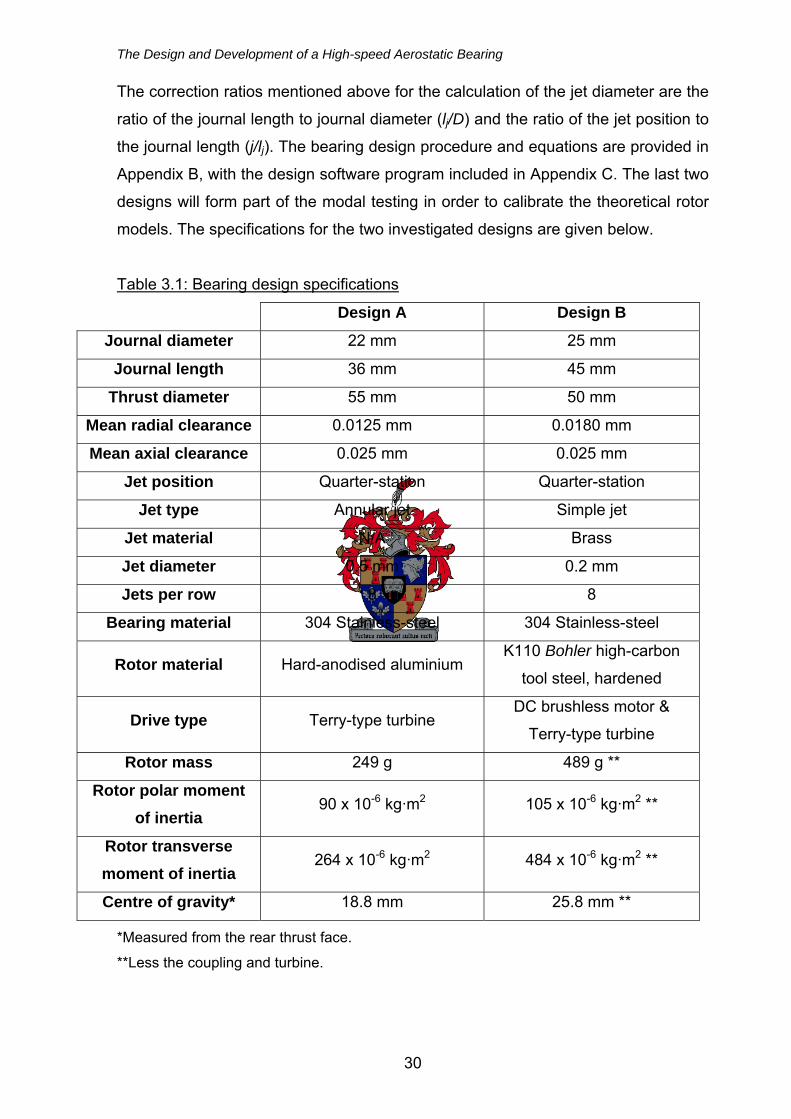
The Design and Development of a High-speed Aerostatic Bearing
The correction ratios mentioned above for the calculation of the jet diameter are the
ratio of the journal length to journal diameter (lj/D) and the ratio of the jet position to
the journal length (j/lj). The bearing design procedure and equations are provided in
Appendix B, with the design software program included in Appendix C. The last two
designs will form part of the modal testing in order to calibrate the theoretical rotor
models. The specifications for the two investigated designs are given below.
Table 3.1: Bearing design specifications
Design A Design B
Journal diameter 22 mm 25 mm
Journal length 36 mm 45 mm
Thrust diameter 55 mm 50 mm
Mean radial clearance 0.0125 mm 0.0180 mm
Mean axial clearance 0.025 mm 0.025 mm
Jet position Quarter-station Quarter-station
Jet type Annular jet Simple jet
Jet material N/A Brass
Jet diameter 0.5 mm 0.2 mm
Jets per row 8 8
Bearing material 304 Stainless-steel 304 Stainless-steel
Rotor material Hard-anodised aluminium K110 Bohler high-carbon
tool steel, hardened
Drive type Terry-type turbine DC brushless motor &
Terry-type turbine
Rotor mass 249 g 489 g **
Rotor polar moment of inertia
90 x 10-6 kg·m2 105 x 10-6 kg·m2 **
Rotor transverse moment of inertia
264 x 10-6 kg·m2 484 x 10-6 kg·m2 **
Centre of gravity* 18.8 mm 25.8 mm **
*Measured from the rear thrust face.
**Less the coupling and turbine.
30
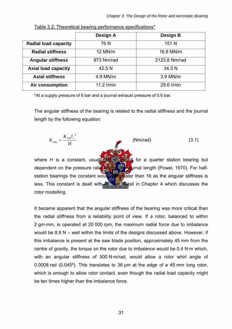
Chapter 3: The Design of the Rotor and Aerostatic Bearing
Table 3.2: Theoretical bearing performance specifications*
Design A Design B
Radial load capacity 76 N 151 N
Radial stiffness 12 MN/m 16.8 MN/m
Angular stiffness 973 Nm/rad 2123.8 Nm/rad
Axial load capacity 42.5 N 34.3 N
Axial stiffness 4.9 MN/m 3.9 MN/m
Air consumption 11.2 l/min 29.6 l/min
*At a supply pressure of 6 bar and a journal exhaust pressure of 0.6 bar.
The angular stiffness of the bearing is related to the radial stiffness and the journal
length by the following equation:
H
lKK jrad
ang
2
= (Nm/rad) (3.1)
where H is a constant, usually taken as 16 for a quarter station bearing but
dependent on the pressure ratio across the journal length (Powel, 1970). For half-
station bearings the constant would be greater than 16 as the angular stiffness is
less. This constant is dealt with in more detail in Chapter 4 which discusses the
rotor modelling.
It became apparent that the angular stiffness of the bearing was more critical than
the radial stiffness from a reliability point of view. If a rotor, balanced to within
2 gm·mm, is operated at 20 000 rpm, the maximum radial force due to imbalance
would be 8.8 N – well within the limits of the designs discussed above. However, if
this imbalance is present at the saw blade position, approximately 45 mm from the
centre of gravity, the torque on the rotor due to imbalance would be 0.4 N·m which,
with an angular stiffness of 500 N·m/rad, would allow a rotor whirl angle of
0.0008 rad (0.045º). This translates to 36 μm at the edge of a 45 mm long rotor,
which is enough to allow rotor contact, even though the radial load capacity might
be ten times higher than the imbalance force.
31
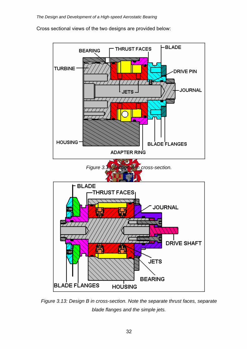
The Design and Development of a High-speed Aerostatic Bearing
Cross sectional views of the two designs are provided below:
Figure 3.12: Design A in cross-section.
Figure 3.13: Design B in cross-section. Note the separate thrust faces, separate
blade flanges and the simple jets.
32
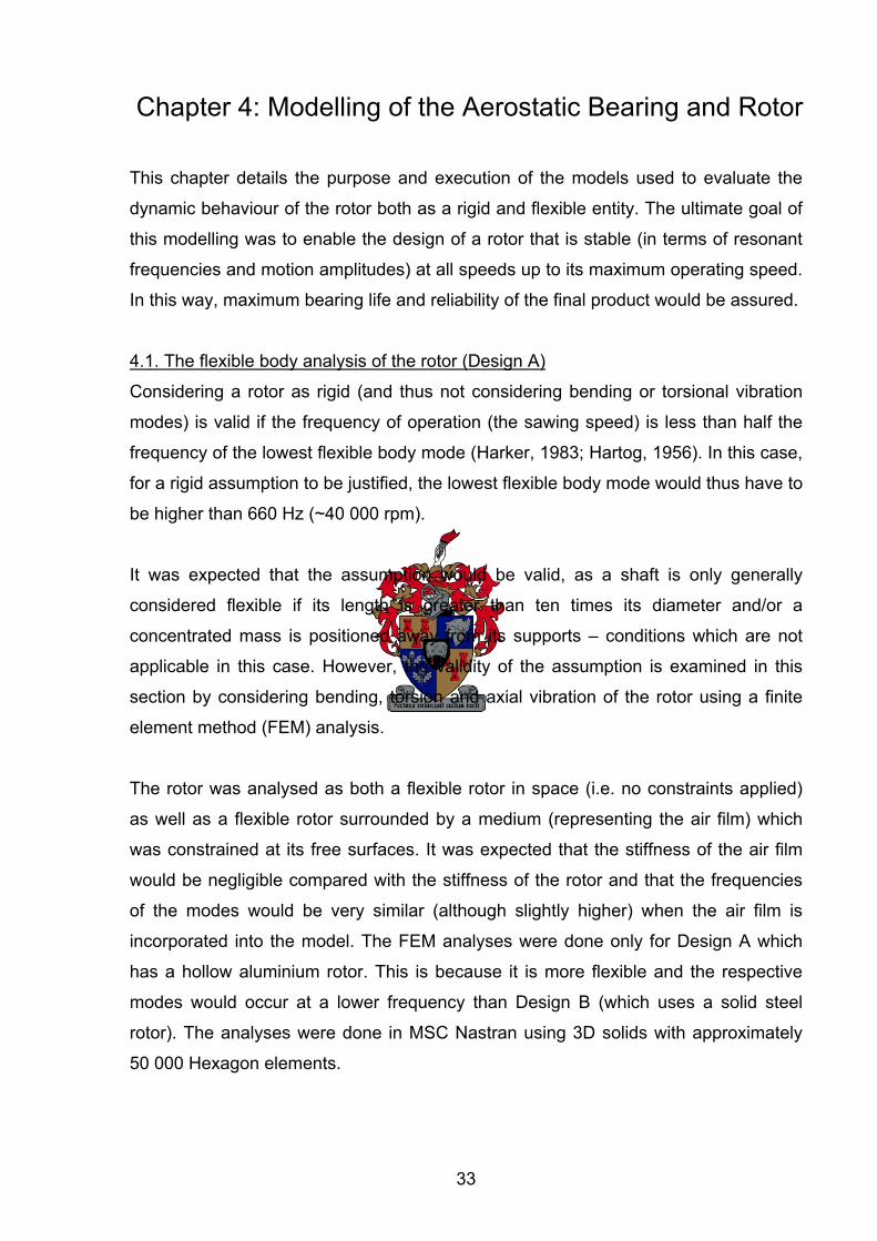
Chapter 4: Modelling of the Aerostatic Bearing and Rotor
This chapter details the purpose and execution of the models used to evaluate the
dynamic behaviour of the rotor both as a rigid and flexible entity. The ultimate goal of
this modelling was to enable the design of a rotor that is stable (in terms of resonant
frequencies and motion amplitudes) at all speeds up to its maximum operating speed.
In this way, maximum bearing life and reliability of the final product would be assured.
4.1. The flexible body analysis of the rotor (Design A)
Considering a rotor as rigid (and thus not considering bending or torsional vibration
modes) is valid if the frequency of operation (the sawing speed) is less than half the
frequency of the lowest flexible body mode (Harker, 1983; Hartog, 1956). In this case,
for a rigid assumption to be justified, the lowest flexible body mode would thus have to
be higher than 660 Hz (~40 000 rpm).
It was expected that the assumption would be valid, as a shaft is only generally
considered flexible if its length is greater than ten times its diameter and/or a
concentrated mass is positioned away from its supports – conditions which are not
applicable in this case. However, the validity of the assumption is examined in this
section by considering bending, torsion and axial vibration of the rotor using a finite
element method (FEM) analysis.
The rotor was analysed as both a flexible rotor in space (i.e. no constraints applied)
as well as a flexible rotor surrounded by a medium (representing the air film) which
was constrained at its free surfaces. It was expected that the stiffness of the air film
would be negligible compared with the stiffness of the rotor and that the frequencies
of the modes would be very similar (although slightly higher) when the air film is
incorporated into the model. The FEM analyses were done only for Design A which
has a hollow aluminium rotor. This is because it is more flexible and the respective
modes would occur at a lower frequency than Design B (which uses a solid steel
rotor). The analyses were done in MSC Nastran using 3D solids with approximately
50 000 Hexagon elements.
33
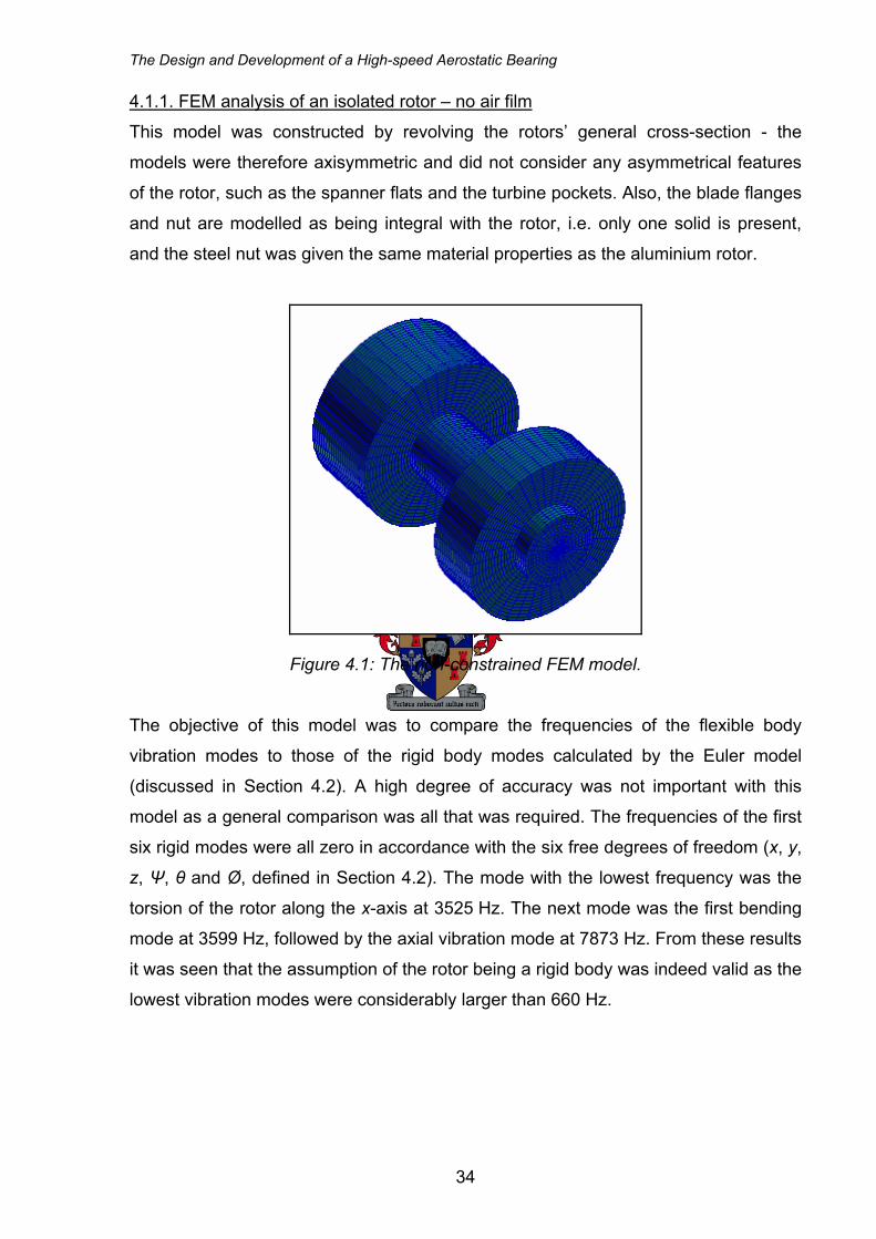
The Design and Development of a High-speed Aerostatic Bearing
4.1.1. FEM analysis of an isolated rotor – no air film
This model was constructed by revolving the rotors’ general cross-section - the
models were therefore axisymmetric and did not consider any asymmetrical features
of the rotor, such as the spanner flats and the turbine pockets. Also, the blade flanges
and nut are modelled as being integral with the rotor, i.e. only one solid is present,
and the steel nut was given the same material properties as the aluminium rotor.
Figure 4.1: The non-constrained FEM model.
The objective of this model was to compare the frequencies of the flexible body
vibration modes to those of the rigid body modes calculated by the Euler model
(discussed in Section 4.2). A high degree of accuracy was not important with this
model as a general comparison was all that was required. The frequencies of the first
six rigid modes were all zero in accordance with the six free degrees of freedom (x, y,
z, Ψ, θ and Ø, defined in Section 4.2). The mode with the lowest frequency was the
torsion of the rotor along the x-axis at 3525 Hz. The next mode was the first bending
mode at 3599 Hz, followed by the axial vibration mode at 7873 Hz. From these results
it was seen that the assumption of the rotor being a rigid body was indeed valid as the
lowest vibration modes were considerably larger than 660 Hz.
34
Chapter 4: Modelling of the Aerostatic Bearing and Rotor
4.1.2. FEM analysis of a supported rotor – with air film
Additional FEM models were built with an ‘air-film’ incorporated. This consisted of an
additional solid with its own unique material properties surrounding the journal.
Figure 4.2: The FEM model incorporating an ‘air film’.
The ‘air film’ solid was shaped so that it represented the fall in air pressure along the
journal. The properties of this ‘air film’ solid were adjusted until the frequencies of the
five rigid body modes (x, y, z, θ and Ø) approximated that of the Euler model. The
FEM analysis calculated an additional axial torsion by considering the shear strength
of the air film which is negligible in reality. The purpose of this FEM analysis was to
determine whether the air film has any significant effect on the modal frequencies of
the free flexible rotor.
The frequencies of the flexible body modes for the constrained model were slightly
higher than that obtained with the free model. Although it was not possible to
construct the model so that it would mimic the results of the Euler model exactly, it
was clear that the effect of the air film was very small.
The results for the frequencies of the rotor’s natural modes obtained from the two
FEM models as well as the Euler model are presented in Table 4.1. Although the
Euler model has yet to be discussed, displaying the results here enables the FEM
results to be put in perspective.
35
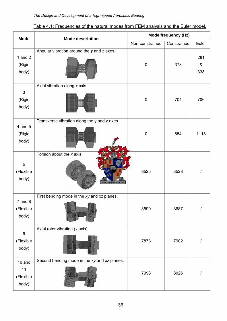
The Design and Development of a High-speed Aerostatic Bearing
Table 4.1: Frequencies of the natural modes from FEM analysis and the Euler model.
Mode frequency (Hz) Mode Mode description
Non-constrained Constrained Euler
1 and 2
(Rigid
body)
Angular vibration around the y and z axes.
0 373
281
&
338
3
(Rigid
body)
Axial vibration along x axis.
0 704 706
4 and 5
(Rigid
body)
Transverse vibration along the y and z axes.
0 854 1113
6
(Flexible
body)
Torsion about the x axis.
3525 3528 /
7 and 8
(Flexible
body)
First bending mode in the xy and xz planes.
3599 3687 /
9
(Flexible
body)
Axial rotor vibration (x axis).
7873 7902 /
10 and
11
(Flexible
body)
Second bending mode in the xy and xz planes.
7998 8026 /
36
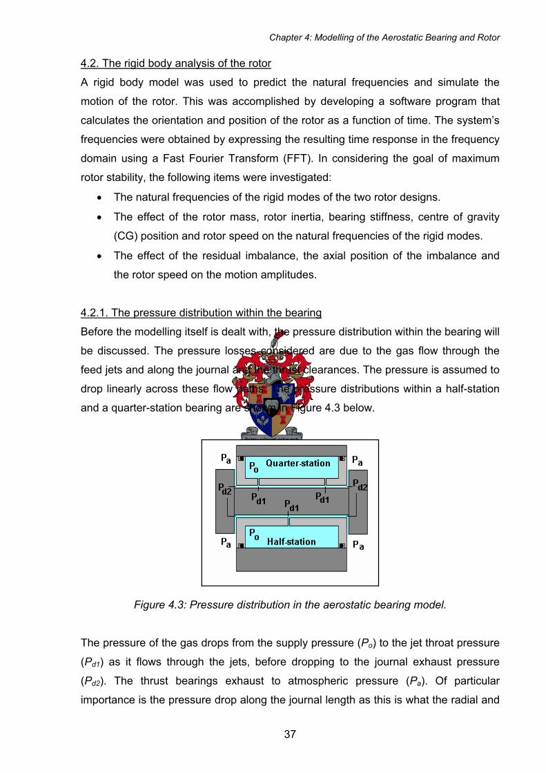
Chapter 4: Modelling of the Aerostatic Bearing and Rotor
4.2. The rigid body analysis of the rotor
A rigid body model was used to predict the natural frequencies and simulate the
motion of the rotor. This was accomplished by developing a software program that
calculates the orientation and position of the rotor as a function of time. The system’s
frequencies were obtained by expressing the resulting time response in the frequency
domain using a Fast Fourier Transform (FFT). In considering the goal of maximum
rotor stability, the following items were investigated:
• The natural frequencies of the rigid modes of the two rotor designs.
• The effect of the rotor mass, rotor inertia, bearing stiffness, centre of gravity
(CG) position and rotor speed on the natural frequencies of the rigid modes.
• The effect of the residual imbalance, the axial position of the imbalance and
the rotor speed on the motion amplitudes.
4.2.1. The pressure distribution within the bearing
Before the modelling itself is dealt with, the pressure distribution within the bearing will
be discussed. The pressure losses considered are due to the gas flow through the
feed jets and along the journal and the thrust clearances. The pressure is assumed to
drop linearly across these flow paths. The pressure distributions within a half-station
and a quarter-station bearing are shown in Figure 4.3 below.
Figure 4.3: Pressure distribution in the aerostatic bearing model.
The pressure of the gas drops from the supply pressure (Po) to the jet throat pressure
(Pd1) as it flows through the jets, before dropping to the journal exhaust pressure
(Pd2). The thrust bearings exhaust to atmospheric pressure (Pa). Of particular
importance is the pressure drop along the journal length as this is what the radial and
37
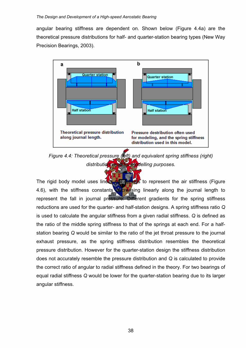
The Design and Development of a High-speed Aerostatic Bearing
angular bearing stiffness are dependent on. Shown below (Figure 4.4a) are the
theoretical pressure distributions for half- and quarter-station bearing types (New Way
Precision Bearings, 2003).
Figure 4.4: Theoretical pressure (left) and equivalent spring stiffness (right)
distribution used for modelling purposes.
The rigid body model uses linear coil springs to represent the air stiffness (Figure
4.6), with the stiffness constants decreasing linearly along the journal length to
represent the fall in journal pressure. Different gradients for the spring stiffness
reductions are used for the quarter- and half-station designs. A spring stiffness ratio Q
is used to calculate the angular stiffness from a given radial stiffness. Q is defined as
the ratio of the middle spring stiffness to that of the springs at each end. For a half-
station bearing Q would be similar to the ratio of the jet throat pressure to the journal
exhaust pressure, as the spring stiffness distribution resembles the theoretical
pressure distribution. However for the quarter-station design the stiffness distribution
does not accurately resemble the pressure distribution and Q is calculated to provide
the correct ratio of angular to radial stiffness defined in the theory. For two bearings of
equal radial stiffness Q would be lower for the quarter-station bearing due to its larger
angular stiffness.
38
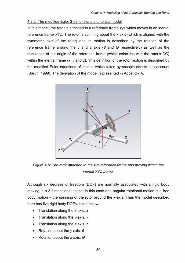
Chapter 4: Modelling of the Aerostatic Bearing and Rotor
4.2.2. The modified Euler 3-dimensional numerical model
In this model, the rotor is attached to a reference frame xyz which moves in an inertial
reference frame XYZ. The rotor is spinning about the x axis (which is aligned with the
symmetric axis of the rotor) and its motion is described by the rotation of the
reference frame around the y and z axis (θ and Ø respectively) as well as the
translation of the origin of the reference frame (which coincides with the rotor’s CG)
within the inertial frame (x, y and z). This definition of the rotor motion is described by
the modified Euler equations of motion which takes gyroscopic effects into account
(Baruh, 1999). The derivation of the model is presented in Appendix A.
Figure 4.5: The rotor attached to the xyz reference frame and moving within the
inertial XYZ frame.
Although six degrees of freedom (DOF) are normally associated with a rigid body
moving in a 3-dimensional space, in this case one angular rotational motion is a free
body motion – the spinning of the rotor around the x-axis. Thus the model described
here has five rigid body DOFs, listed below:
• Translation along the x-axis, x
• Translation along the y-axis, y
• Translation along the z-axis, z
• Rotation about the y-axis, θ
• Rotation about the z-axis, Ø
39
The Design and Development of a High-speed Aerostatic Bearing
The corresponding equations of motion are (as derived in Appendix A):
( ) ( )[ ]( ) ( )( zyx
cutfricaxax
vvmMvMtetetetem
WFFtntnBxCxKiF
θφψψφψψθψφψθ )φφθθαψψ
&&&&&&&&&&&&&&&
&&&
+−+=−−−−
−−++−+−−Σ
cos2sin2sincos
sinsin:)( (4.1)
( ) ( )[ ]( ) ( )( zxycutfric
dampradrad
vvmMvMteamWFF
tntnBCyCyKjF
φθφψψφθφ
θφαψψφφ&&&&&&&
&&&&
−−+=−−−−−
+−−Σ−−Γ−−Σ
sin
sinsin:)(2 ) (4.2)
( ) ( ) ( )[ ]( ) ( )( )yxzfric
dampradrad
vvmMvMteamF
tntnBCzCzKkF
φθθψψθ
αψψθφφθθ&&&&&&&
&&&&&
+−−+=−−−
+−−Σ−+−Γ+−Σ
cos
sinsin:)(2
(4.3)
( ) ( ) ( )( )[ ] ( )( ) ( )φθφθψψψψθ
ψψψφαωω&&&&&&&&&&&&
&&&&&&
++=−+−
−++++Σ
xxz
yt
Iteteavm
teteavmtntnBriM
sincos
cossinsinsin:2
2
(4.4)
( ) ( ) ( ) ( )[ ]( ) ( )
( ) ( ) ( ) ( )φθφψφφθφφφθθψ
ψψψφψψθψφψψμ
ωαωθφφθθ
&&&&&&&&&&&
&&&&&&&&&&&&&&
&&&
zzxxyyyy
xzcut
dampdampang
IIItmemaI
tetetetevmtevamFh
tntncBCCzKzjM
−++−+−=
−−−−−++
−++ΣΣ−−Σ+−ΓΣ
222
2
cos
coscos2sin2sincos
sinsin: (4.5)
( ) ( ) ( )[ ]( ) ( )( )[ ]( )
( ) ( ) ( ) ( ψθφθφθψφψψ
ψψψφψψθψθθμ
θφμφθαψψ
θφαψψφφ
&&&&&&&&&&
&&&&&&&&&&&
&&
&&&&
+−+++=−−
−−++−
−−+++++
+−+ΣΣ−Σ−−Γ−Σ
222222 sinsin
sincos..2sin..2cos.
sinsin2
sinsin:
xxyyzzy
xcutb
cutcutcutbt
dampdampang
IImatmeItevam
tetetetevmFr
FhhFFrtntnBEr
tntncBCCyKykM
) (4.6)
The rotor is modelled as a geometrically-uniform shaft with a non-symmetric CG. A
mass imbalance is incorporated into the model at an axial distance a from the CG and
a radial distance e from the journal axis. The springs and viscous dampers
representing the air film support the journal axially as well as radially. The stiffness
and damping coefficients are independent of the rotor displacement and velocity
respectively, i.e. they exhibit linear behaviour.
40
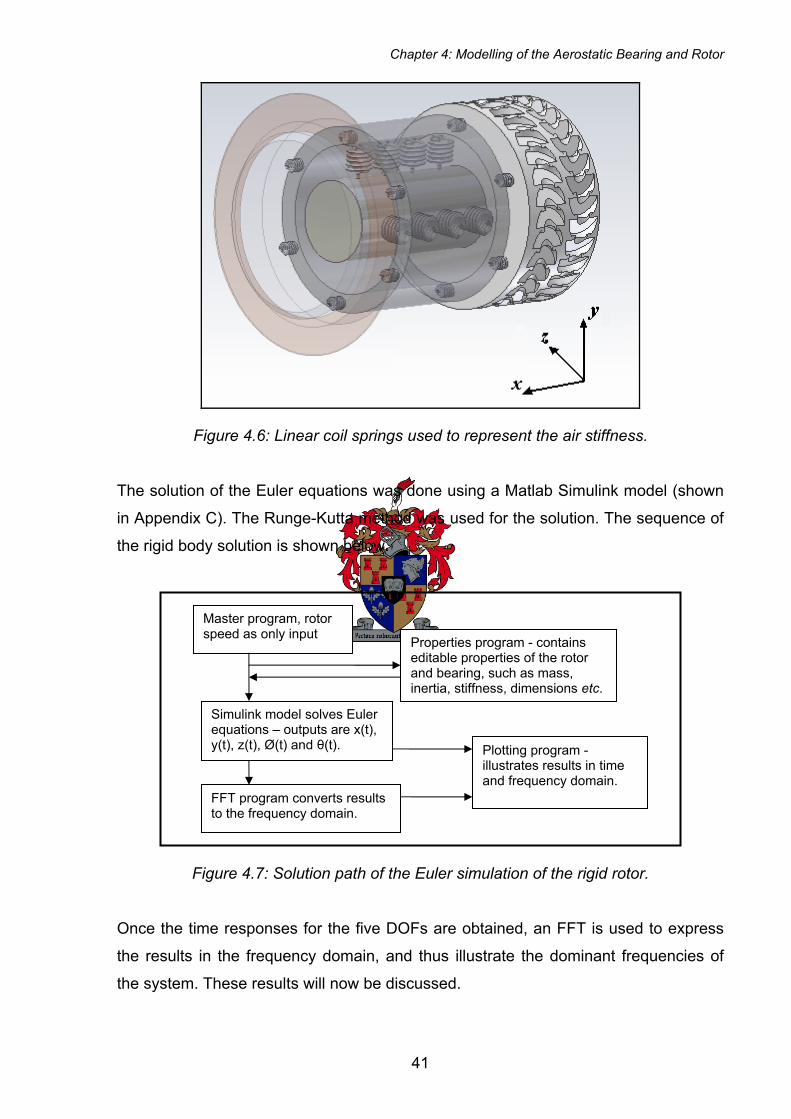
Chapter 4: Modelling of the Aerostatic Bearing and Rotor
Figure 4.6: Linear coil springs used to represent the air stiffness.
The solution of the Euler equations was done using a Matlab Simulink model (shown
in Appendix C). The Runge-Kutta method was used for the solution. The sequence of
the rigid body solution is shown below.
Master program, rotor speed as only input Properties program - contains
editable properties of the rotor and bearing, such as mass, inertia, stiffness, dimensions etc.
Simulink model solves Euler equations – outputs are x(t), y(t), z(t), Ø(t) and θ(t). Plotting program -
illustrates results in time and frequency domain.
FFT program converts results to the frequency domain.
Figure 4.7: Solution path of the Euler simulation of the rigid rotor.
Once the time responses for the five DOFs are obtained, an FFT is used to express
the results in the frequency domain, and thus illustrate the dominant frequencies of
the system. These results will now be discussed.
41
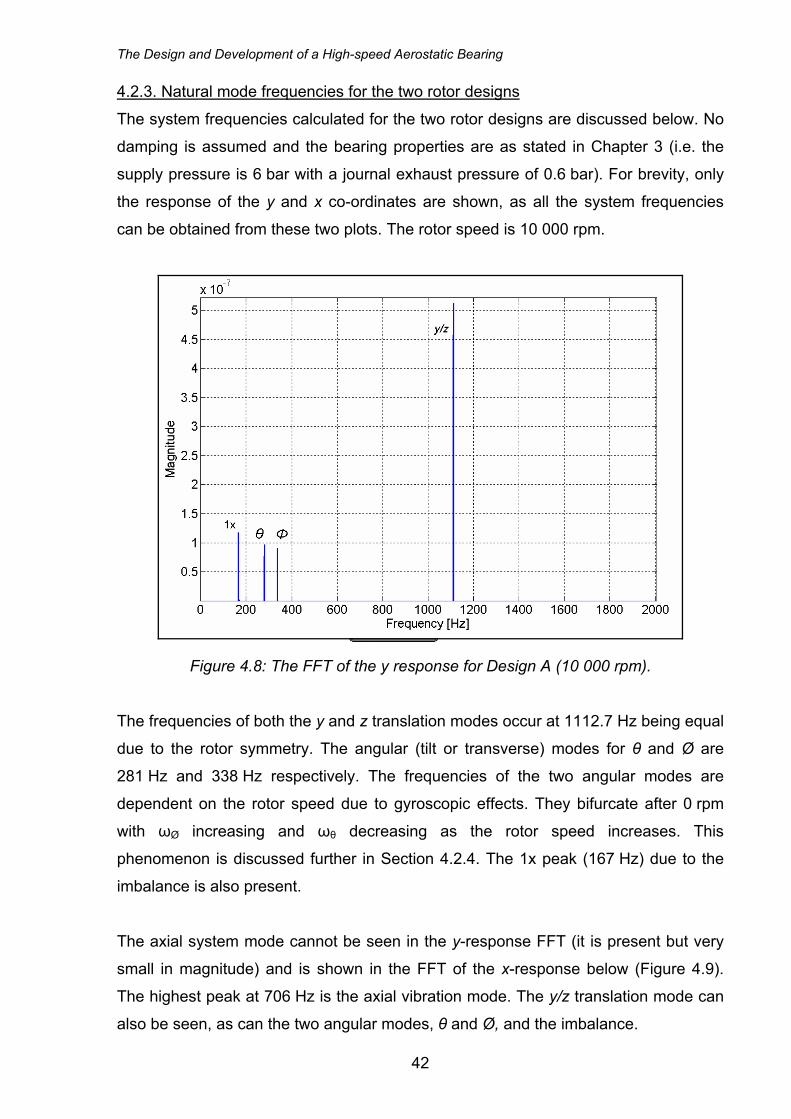
The Design and Development of a High-speed Aerostatic Bearing
4.2.3. Natural mode frequencies for the two rotor designs
The system frequencies calculated for the two rotor designs are discussed below. No
damping is assumed and the bearing properties are as stated in Chapter 3 (i.e. the
supply pressure is 6 bar with a journal exhaust pressure of 0.6 bar). For brevity, only
the response of the y and x co-ordinates are shown, as all the system frequencies
can be obtained from these two plots. The rotor speed is 10 000 rpm.
Figure 4.8: The FFT of the y response for Design A (10 000 rpm).
The frequencies of both the y and z translation modes occur at 1112.7 Hz being equal
due to the rotor symmetry. The angular (tilt or transverse) modes for θ and Ø are
281 Hz and 338 Hz respectively. The frequencies of the two angular modes are
dependent on the rotor speed due to gyroscopic effects. They bifurcate after 0 rpm
with ωØ increasing and ωθ decreasing as the rotor speed increases. This
phenomenon is discussed further in Section 4.2.4. The 1x peak (167 Hz) due to the
imbalance is also present.
The axial system mode cannot be seen in the y-response FFT (it is present but very
small in magnitude) and is shown in the FFT of the x-response below (Figure 4.9).
The highest peak at 706 Hz is the axial vibration mode. The y/z translation mode can
also be seen, as can the two angular modes, θ and Ø, and the imbalance.
42
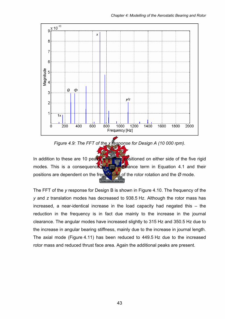
Chapter 4: Modelling of the Aerostatic Bearing and Rotor
Figure 4.9: The FFT of the x response for Design A (10 000 rpm).
In addition to these are 10 peaks which are positioned on either side of the five rigid
modes. This is a consequence of the imbalance term in Equation 4.1 and their
positions are dependent on the frequencies of the rotor rotation and the Ø mode.
The FFT of the y response for Design B is shown in Figure 4.10. The frequency of the
y and z translation modes has decreased to 938.5 Hz. Although the rotor mass has
increased, a near-identical increase in the load capacity had negated this – the
reduction in the frequency is in fact due mainly to the increase in the journal
clearance. The angular modes have increased slightly to 315 Hz and 350.5 Hz due to
the increase in angular bearing stiffness, mainly due to the increase in journal length.
The axial mode (Figure 4.11) has been reduced to 449.5 Hz due to the increased
rotor mass and reduced thrust face area. Again the additional peaks are present.
43
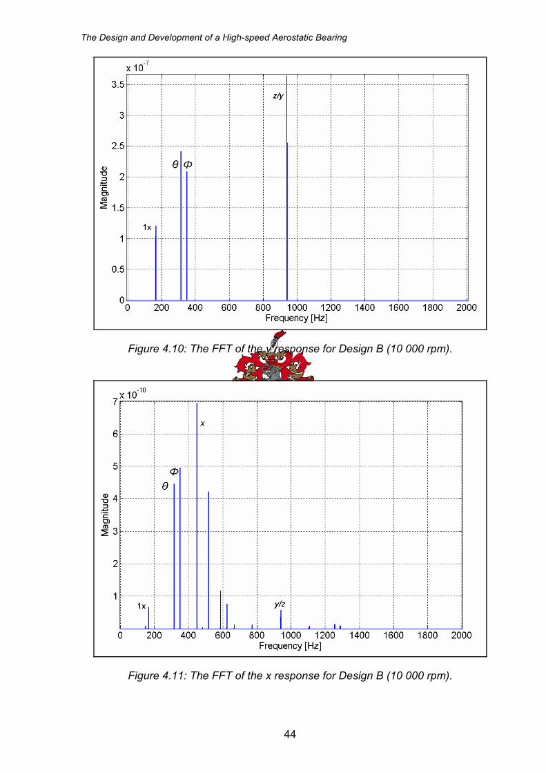
The Design and Development of a High-speed Aerostatic Bearing
Figure 4.10: The FFT of the y response for Design B (10 000 rpm).
Figure 4.11: The FFT of the x response for Design B (10 000 rpm).
44
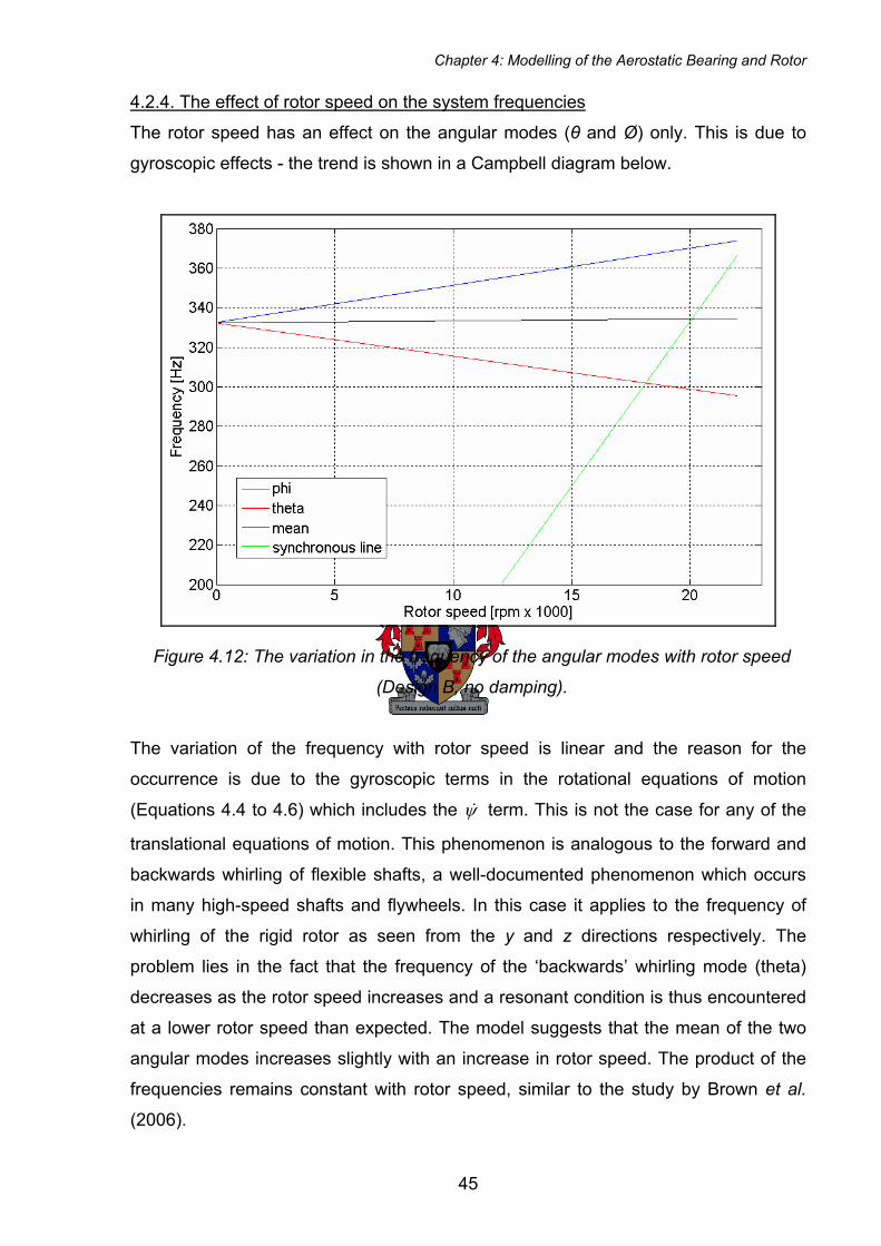
Chapter 4: Modelling of the Aerostatic Bearing and Rotor
4.2.4. The effect of rotor speed on the system frequencies
The rotor speed has an effect on the angular modes (θ and Ø) only. This is due to
gyroscopic effects - the trend is shown in a Campbell diagram below.
Figure 4.12: The variation in the frequency of the angular modes with rotor speed
(Design B, no damping).
The variation of the frequency with rotor speed is linear and the reason for the
occurrence is due to the gyroscopic terms in the rotational equations of motion
(Equations 4.4 to 4.6) which includes the ψ& term. This is not the case for any of the
translational equations of motion. This phenomenon is analogous to the forward and
backwards whirling of flexible shafts, a well-documented phenomenon which occurs
in many high-speed shafts and flywheels. In this case it applies to the frequency of
whirling of the rigid rotor as seen from the y and z directions respectively. The
problem lies in the fact that the frequency of the ‘backwards’ whirling mode (theta)
decreases as the rotor speed increases and a resonant condition is thus encountered
at a lower rotor speed than expected. The model suggests that the mean of the two
angular modes increases slightly with an increase in rotor speed. The product of the
frequencies remains constant with rotor speed, similar to the study by Brown et al.
(2006).
45
The Design and Development of a High-speed Aerostatic Bearing
4.2.5. The effect of rotor mass, rotor inertia, bearing stiffness and the position of the
centre of gravity on the system frequencies
The effect of rotor mass, rotor inertia and bearing stiffness on the system frequencies
is similar to that of single degree of freedom (SDOF) vibration theory (Inman, 2001).
The frequency of the axial vibration mode given by the Euler model is exactly as that
given by SDOF theory and is independent on the position of the CG. That is, the
frequency of the axial mode can be calculated by the equation:
π
ω2MKax
x = (Hz) (4.7)
The y and z transverse vibration frequency is slightly higher than that given by SDOF
theory, due to the non-symmetric position of the CG. This variation is very small –
less than 1% change in frequency for a 15% change in the distance of gravity position
from the journal end. If the CG is positioned in the geometric centre of the journal, the
Euler model and SDOF theory give the same frequencies and thus can be defined by
the equation:
πω
2,M
Krad
zy = (Hz) (4.8)
Considering the fact that the frequencies of the angular modes change with the rotor
speed, it is necessary to compare the mean frequency of the two modes with the
single frequency calculated from SDOF theory. This mean value also increases
slightly with rotor speed, as seen in Figure 4.12. When the CG of the rotor and the
geometric centre of the journal coincide, the SDOF theory and Euler model give the
same results at 0 rpm – that is, the frequency defined by the following equation:
πω φθ 2,
zz
ang
IK
= (Hz) (4.9)
46
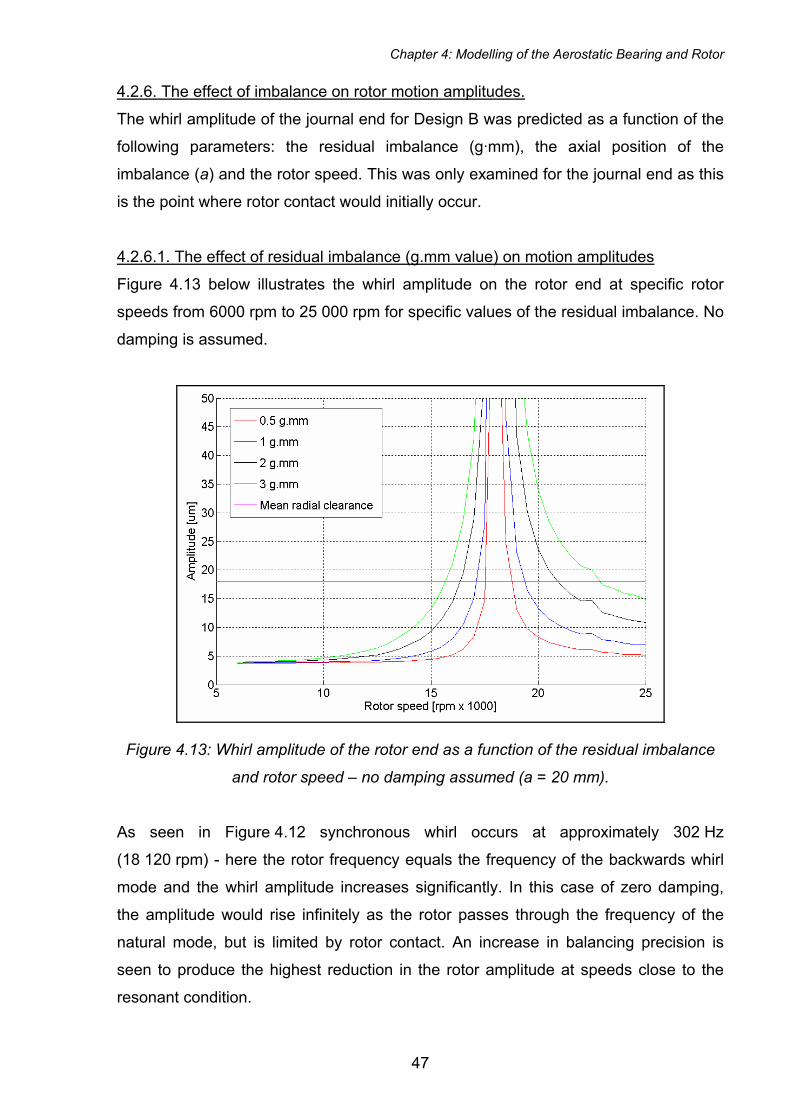
Chapter 4: Modelling of the Aerostatic Bearing and Rotor
4.2.6. The effect of imbalance on rotor motion amplitudes.
The whirl amplitude of the journal end for Design B was predicted as a function of the
following parameters: the residual imbalance (g·mm), the axial position of the
imbalance (a) and the rotor speed. This was only examined for the journal end as this
is the point where rotor contact would initially occur.
4.2.6.1. The effect of residual imbalance (g.mm value) on motion amplitudes
Figure 4.13 below illustrates the whirl amplitude on the rotor end at specific rotor
speeds from 6000 rpm to 25 000 rpm for specific values of the residual imbalance. No
damping is assumed.
Figure 4.13: Whirl amplitude of the rotor end as a function of the residual imbalance
and rotor speed – no damping assumed (a = 20 mm).
As seen in Figure 4.12 synchronous whirl occurs at approximately 302 Hz
(18 120 rpm) - here the rotor frequency equals the frequency of the backwards whirl
mode and the whirl amplitude increases significantly. In this case of zero damping,
the amplitude would rise infinitely as the rotor passes through the frequency of the
natural mode, but is limited by rotor contact. An increase in balancing precision is
seen to produce the highest reduction in the rotor amplitude at speeds close to the
resonant condition.
47
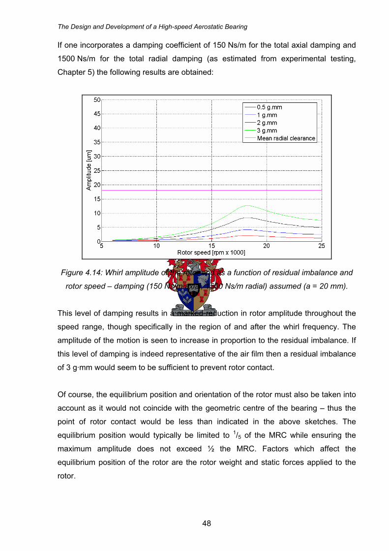
The Design and Development of a High-speed Aerostatic Bearing
If one incorporates a damping coefficient of 150 Ns/m for the total axial damping and
1500 Ns/m for the total radial damping (as estimated from experimental testing,
Chapter 5) the following results are obtained:
Figure 4.14: Whirl amplitude of the rotor end as a function of residual imbalance and
rotor speed – damping (150 Ns/m axial, 1500 Ns/m radial) assumed (a = 20 mm).
This level of damping results in a marked reduction in rotor amplitude throughout the
speed range, though specifically in the region of and after the whirl frequency. The
amplitude of the motion is seen to increase in proportion to the residual imbalance. If
this level of damping is indeed representative of the air film then a residual imbalance
of 3 g·mm would seem to be sufficient to prevent rotor contact.
Of course, the equilibrium position and orientation of the rotor must also be taken into
account as it would not coincide with the geometric centre of the bearing – thus the
point of rotor contact would be less than indicated in the above sketches. The
equilibrium position would typically be limited to 1/5 of the MRC while ensuring the
maximum amplitude does not exceed ½ the MRC. Factors which affect the
equilibrium position of the rotor are the rotor weight and static forces applied to the
rotor.
48
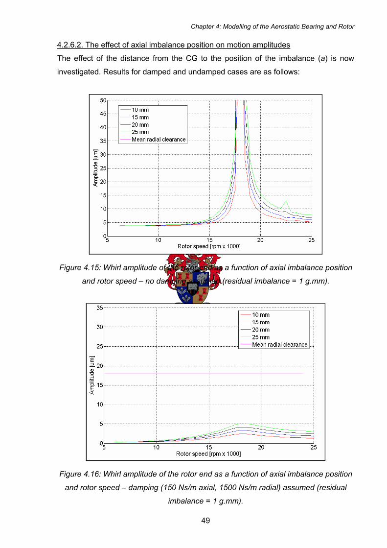
Chapter 4: Modelling of the Aerostatic Bearing and Rotor
4.2.6.2. The effect of axial imbalance position on motion amplitudes
The effect of the distance from the CG to the position of the imbalance (a) is now
investigated. Results for damped and undamped cases are as follows:
Figure 4.15: Whirl amplitude of the rotor end as a function of axial imbalance position
and rotor speed – no damping assumed (residual imbalance = 1 g.mm).
Figure 4.16: Whirl amplitude of the rotor end as a function of axial imbalance position
and rotor speed – damping (150 Ns/m axial, 1500 Ns/m radial) assumed (residual
imbalance = 1 g.mm).
49
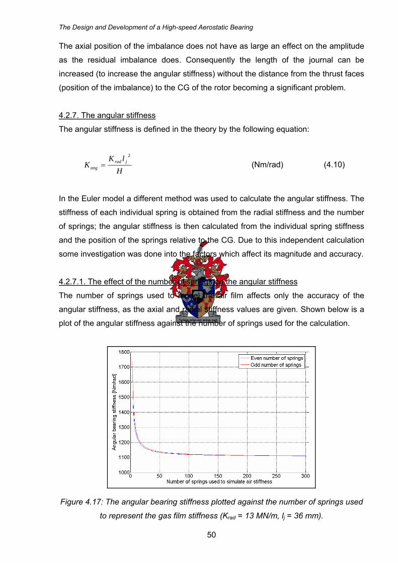
The Design and Development of a High-speed Aerostatic Bearing
The axial position of the imbalance does not have as large an effect on the amplitude
as the residual imbalance does. Consequently the length of the journal can be
increased (to increase the angular stiffness) without the distance from the thrust faces
(position of the imbalance) to the CG of the rotor becoming a significant problem.
4.2.7. The angular stiffness
The angular stiffness is defined in the theory by the following equation:
H
lKK jrad
ang
2
= (Nm/rad) (4.10)
In the Euler model a different method was used to calculate the angular stiffness. The
stiffness of each individual spring is obtained from the radial stiffness and the number
of springs; the angular stiffness is then calculated from the individual spring stiffness
and the position of the springs relative to the CG. Due to this independent calculation
some investigation was done into the factors which affect its magnitude and accuracy.
4.2.7.1. The effect of the number of springs on the angular stiffness
The number of springs used to model the air film affects only the accuracy of the
angular stiffness, as the axial and radial stiffness values are given. Shown below is a
plot of the angular stiffness against the number of springs used for the calculation.
Figure 4.17: The angular bearing stiffness plotted against the number of springs used
to represent the gas film stiffness (Krad = 13 MN/m, lj = 36 mm).
50
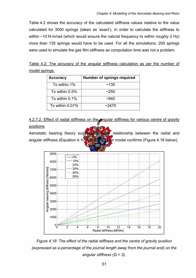
Chapter 4: Modelling of the Aerostatic Bearing and Rotor
Table 4.2 shows the accuracy of the calculated stiffness values relative to the value
calculated for 3000 springs (taken as ‘exact’). In order to calculate the stiffness to
within ~10 N·m/rad (which would ensure the natural frequency to within roughly 2 Hz)
more than 135 springs would have to be used. For all the simulations, 200 springs
were used to simulate the gas film stiffness as computation time was not a problem.
Table 4.2: The accuracy of the angular stiffness calculation as per the number of
model springs.
Accuracy Number of springs required
To within 1% ~135
To within 0.5% ~250
To within 0.1% ~940
To within 0.01% ~2470
4.2.7.2. Effect of radial stiffness on the angular stiffness for various centre of gravity
positions
Aerostatic bearing theory suggests a linear relationship between the radial and
angular stiffness (Equation 4.10) which the Euler model confirms (Figure 4.18 below).
Figure 4.18: The effect of the radial stiffness and the centre of gravity position
(expressed as a percentage of the journal length away from the journal end) on the
angular stiffness (Q = 3).
51
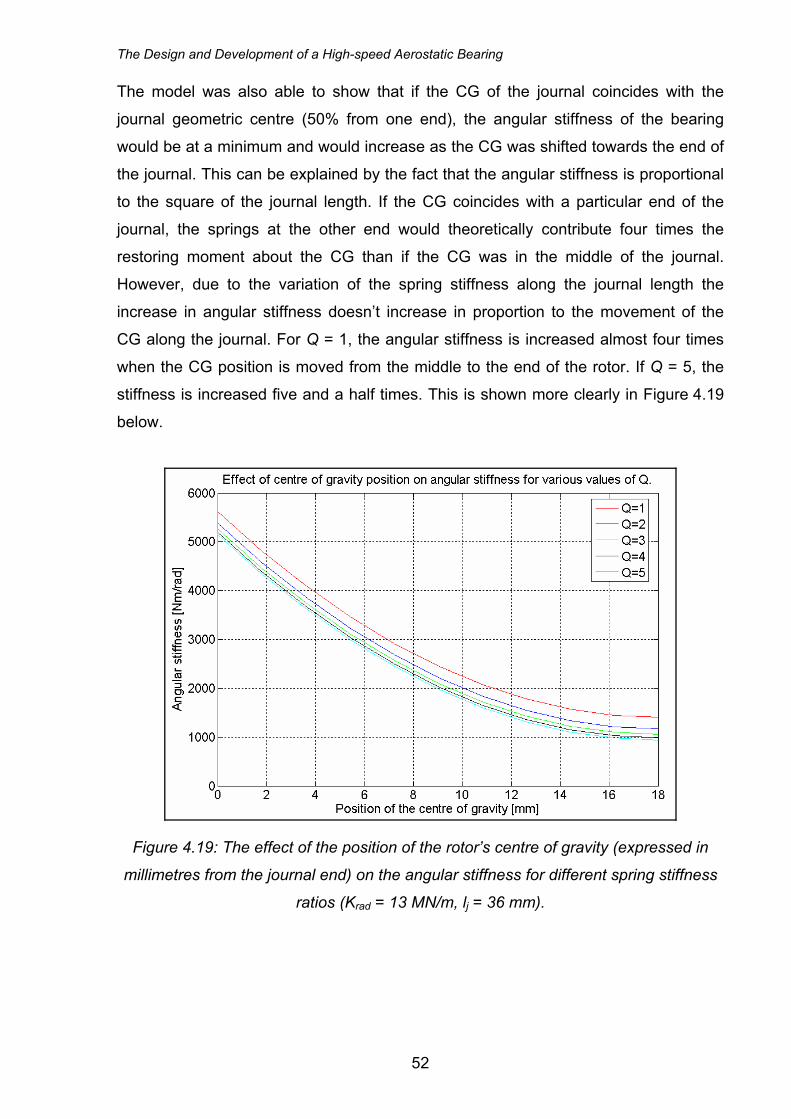
The Design and Development of a High-speed Aerostatic Bearing
The model was also able to show that if the CG of the journal coincides with the
journal geometric centre (50% from one end), the angular stiffness of the bearing
would be at a minimum and would increase as the CG was shifted towards the end of
the journal. This can be explained by the fact that the angular stiffness is proportional
to the square of the journal length. If the CG coincides with a particular end of the
journal, the springs at the other end would theoretically contribute four times the
restoring moment about the CG than if the CG was in the middle of the journal.
However, due to the variation of the spring stiffness along the journal length the
increase in angular stiffness doesn’t increase in proportion to the movement of the
CG along the journal. For Q = 1, the angular stiffness is increased almost four times
when the CG position is moved from the middle to the end of the rotor. If Q = 5, the
stiffness is increased five and a half times. This is shown more clearly in Figure 4.19
below.
Figure 4.19: The effect of the position of the rotor’s centre of gravity (expressed in
millimetres from the journal end) on the angular stiffness for different spring stiffness
ratios (Krad = 13 MN/m, lj = 36 mm).
52
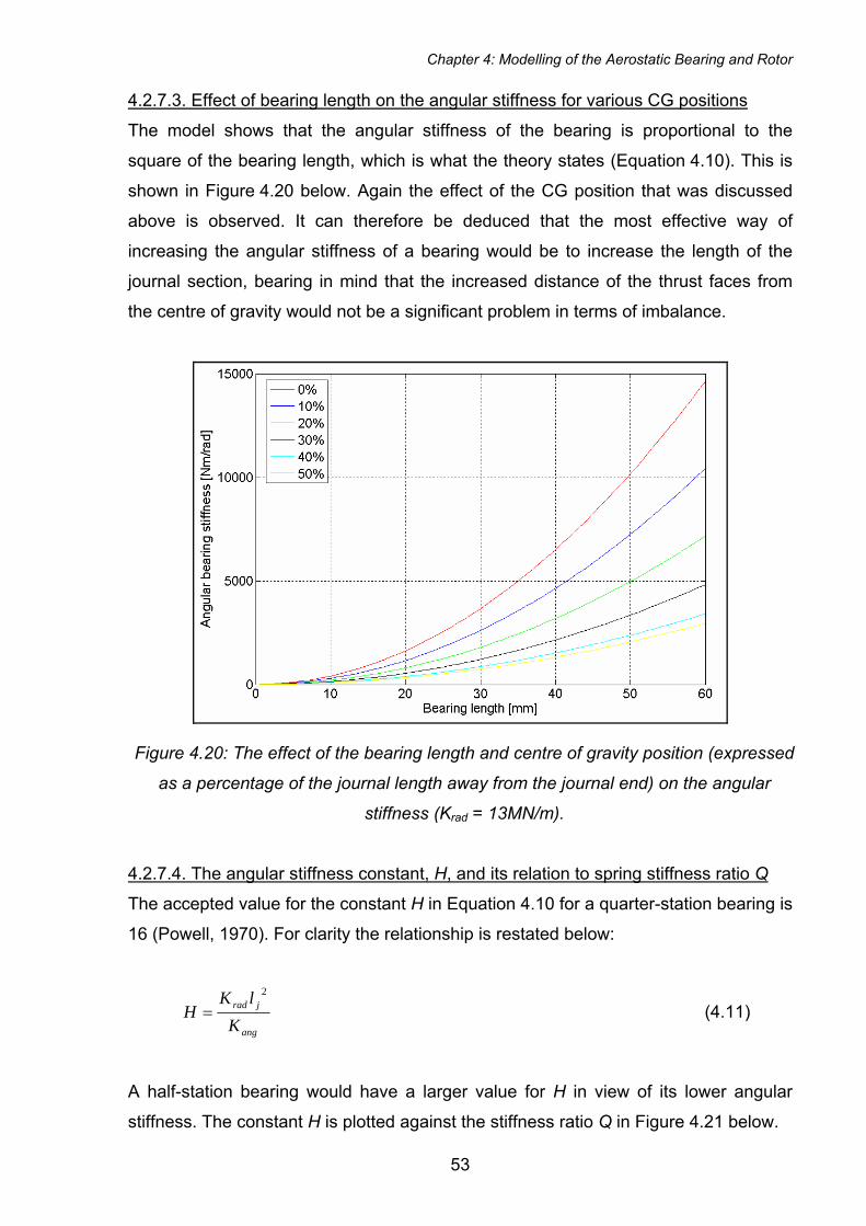
Chapter 4: Modelling of the Aerostatic Bearing and Rotor
4.2.7.3. Effect of bearing length on the angular stiffness for various CG positions
The model shows that the angular stiffness of the bearing is proportional to the
square of the bearing length, which is what the theory states (Equation 4.10). This is
shown in Figure 4.20 below. Again the effect of the CG position that was discussed
above is observed. It can therefore be deduced that the most effective way of
increasing the angular stiffness of a bearing would be to increase the length of the
journal section, bearing in mind that the increased distance of the thrust faces from
the centre of gravity would not be a significant problem in terms of imbalance.
Figure 4.20: The effect of the bearing length and centre of gravity position (expressed
as a percentage of the journal length away from the journal end) on the angular
stiffness (Krad = 13MN/m).
4.2.7.4. The angular stiffness constant, H, and its relation to spring stiffness ratio Q
The accepted value for the constant H in Equation 4.10 for a quarter-station bearing is
16 (Powell, 1970). For clarity the relationship is restated below:
ang
jrad
KlK
H2
= (4.11)
A half-station bearing would have a larger value for H in view of its lower angular
stiffness. The constant H is plotted against the stiffness ratio Q in Figure 4.21 below.
53
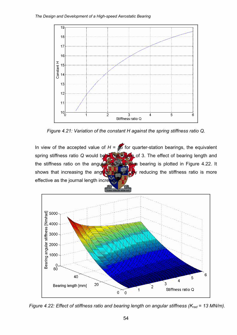
The Design and Development of a High-speed Aerostatic Bearing
Figure 4.21: Variation of the constant H against the spring stiffness ratio Q.
In view of the accepted value of H = 16 for quarter-station bearings, the equivalent
spring stiffness ratio Q would be in the region of 3. The effect of bearing length and
the stiffness ratio on the angular stiffness of a bearing is plotted in Figure 4.22. It
shows that increasing the angular stiffness by reducing the stiffness ratio is more
effective as the journal length increases.
Figure 4.22: Effect of stiffness ratio and bearing length on angular stiffness (Krad = 13 MN/m).
54
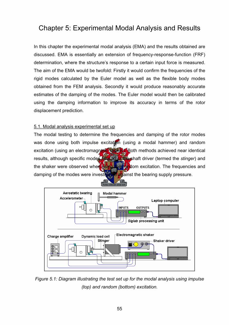
Chapter 5: Experimental Modal Analysis and Results
In this chapter the experimental modal analysis (EMA) and the results obtained are
discussed. EMA is essentially an extension of frequency-response-function (FRF)
determination, where the structure’s response to a certain input force is measured.
The aim of the EMA would be twofold: Firstly it would confirm the frequencies of the
rigid modes calculated by the Euler model as well as the flexible body modes
obtained from the FEM analysis. Secondly it would produce reasonably accurate
estimates of the damping of the modes. The Euler model would then be calibrated
using the damping information to improve its accuracy in terms of the rotor
displacement prediction.
5.1. Modal analysis experimental set up
The modal testing to determine the frequencies and damping of the rotor modes
was done using both impulse excitation (using a modal hammer) and random
excitation (using an electromagnetic shaker). Both methods achieved near identical
results, although specific modes related to the shaft driver (termed the stinger) and
the shaker were observed when using the random excitation. The frequencies and
damping of the modes were investigated against the bearing supply pressure.
Figure 5.1: Diagram illustrating the test set up for the modal analysis using impulse
(top) and random (bottom) excitation.
55
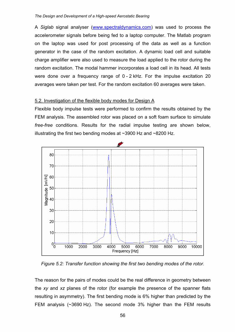
The Design and Development of a High-speed Aerostatic Bearing
A Siglab signal analyser (www.spectraldynamics.com) was used to process the
accelerometer signals before being fed to a laptop computer. The Matlab program
on the laptop was used for post processing of the data as well as a function
generator in the case of the random excitation. A dynamic load cell and suitable
charge amplifier were also used to measure the load applied to the rotor during the
random excitation. The modal hammer incorporates a load cell in its head. All tests
were done over a frequency range of 0 - 2 kHz. For the impulse excitation 20
averages were taken per test. For the random excitation 60 averages were taken.
5.2. Investigation of the flexible body modes for Design A
Flexible body impulse tests were performed to confirm the results obtained by the
FEM analysis. The assembled rotor was placed on a soft foam surface to simulate
free-free conditions. Results for the radial impulse testing are shown below,
illustrating the first two bending modes at ~3900 Hz and ~8200 Hz.
Figure 5.2: Transfer function showing the first two bending modes of the rotor.
The reason for the pairs of modes could be the real difference in geometry between
the xy and xz planes of the rotor (for example the presence of the spanner flats
resulting in asymmetry). The first bending mode is 6% higher than predicted by the
FEM analysis (~3690 Hz). The second mode 3% higher than the FEM results
56
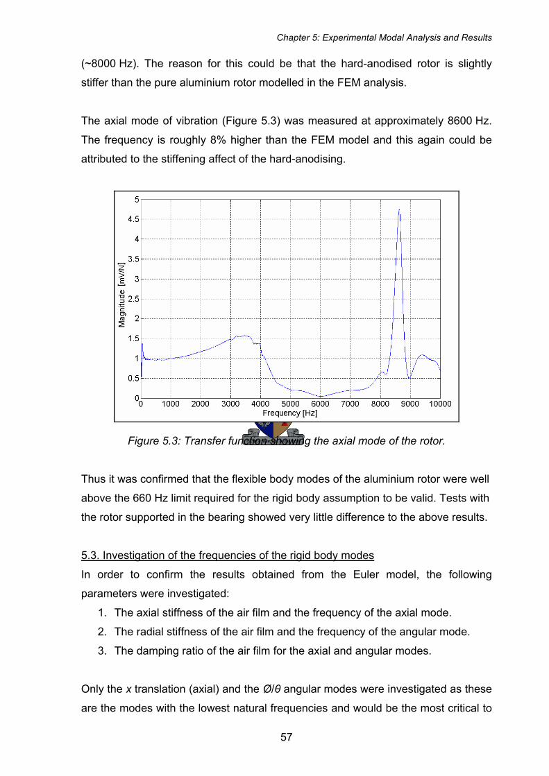
Chapter 5: Experimental Modal Analysis and Results
(~8000 Hz). The reason for this could be that the hard-anodised rotor is slightly
stiffer than the pure aluminium rotor modelled in the FEM analysis.
The axial mode of vibration (Figure 5.3) was measured at approximately 8600 Hz.
The frequency is roughly 8% higher than the FEM model and this again could be
attributed to the stiffening affect of the hard-anodising.
Figure 5.3: Transfer function showing the axial mode of the rotor.
Thus it was confirmed that the flexible body modes of the aluminium rotor were well
above the 660 Hz limit required for the rigid body assumption to be valid. Tests with
the rotor supported in the bearing showed very little difference to the above results.
5.3. Investigation of the frequencies of the rigid body modes
In order to confirm the results obtained from the Euler model, the following
parameters were investigated:
1. The axial stiffness of the air film and the frequency of the axial mode.
2. The radial stiffness of the air film and the frequency of the angular mode.
3. The damping ratio of the air film for the axial and angular modes.
Only the x translation (axial) and the Ø/θ angular modes were investigated as these
are the modes with the lowest natural frequencies and would be the most critical to
57
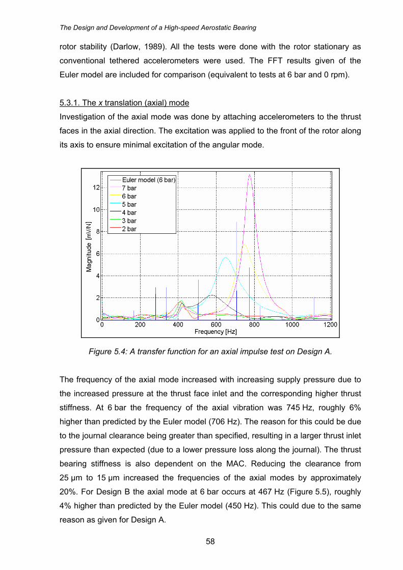
The Design and Development of a High-speed Aerostatic Bearing
rotor stability (Darlow, 1989). All the tests were done with the rotor stationary as
conventional tethered accelerometers were used. The FFT results given of the
Euler model are included for comparison (equivalent to tests at 6 bar and 0 rpm).
5.3.1. The x translation (axial) mode
Investigation of the axial mode was done by attaching accelerometers to the thrust
faces in the axial direction. The excitation was applied to the front of the rotor along
its axis to ensure minimal excitation of the angular mode.
Figure 5.4: A transfer function for an axial impulse test on Design A.
The frequency of the axial mode increased with increasing supply pressure due to
the increased pressure at the thrust face inlet and the corresponding higher thrust
stiffness. At 6 bar the frequency of the axial vibration was 745 Hz, roughly 6%
higher than predicted by the Euler model (706 Hz). The reason for this could be due
to the journal clearance being greater than specified, resulting in a larger thrust inlet
pressure than expected (due to a lower pressure loss along the journal). The thrust
bearing stiffness is also dependent on the MAC. Reducing the clearance from
25 μm to 15 µm increased the frequencies of the axial modes by approximately
20%. For Design B the axial mode at 6 bar occurs at 467 Hz (Figure 5.5), roughly
4% higher than predicted by the Euler model (450 Hz). This could due to the same
reason as given for Design A.
58
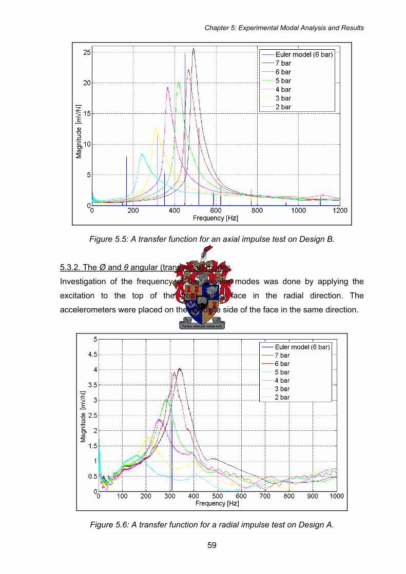
Chapter 5: Experimental Modal Analysis and Results
Figure 5.5: A transfer function for an axial impulse test on Design B.
5.3.2. The Ø and θ angular (transverse) modes
Investigation of the frequency of the angular modes was done by applying the
excitation to the top of the front thrust face in the radial direction. The
accelerometers were placed on the opposite side of the face in the same direction.
Figure 5.6: A transfer function for a radial impulse test on Design A.
59
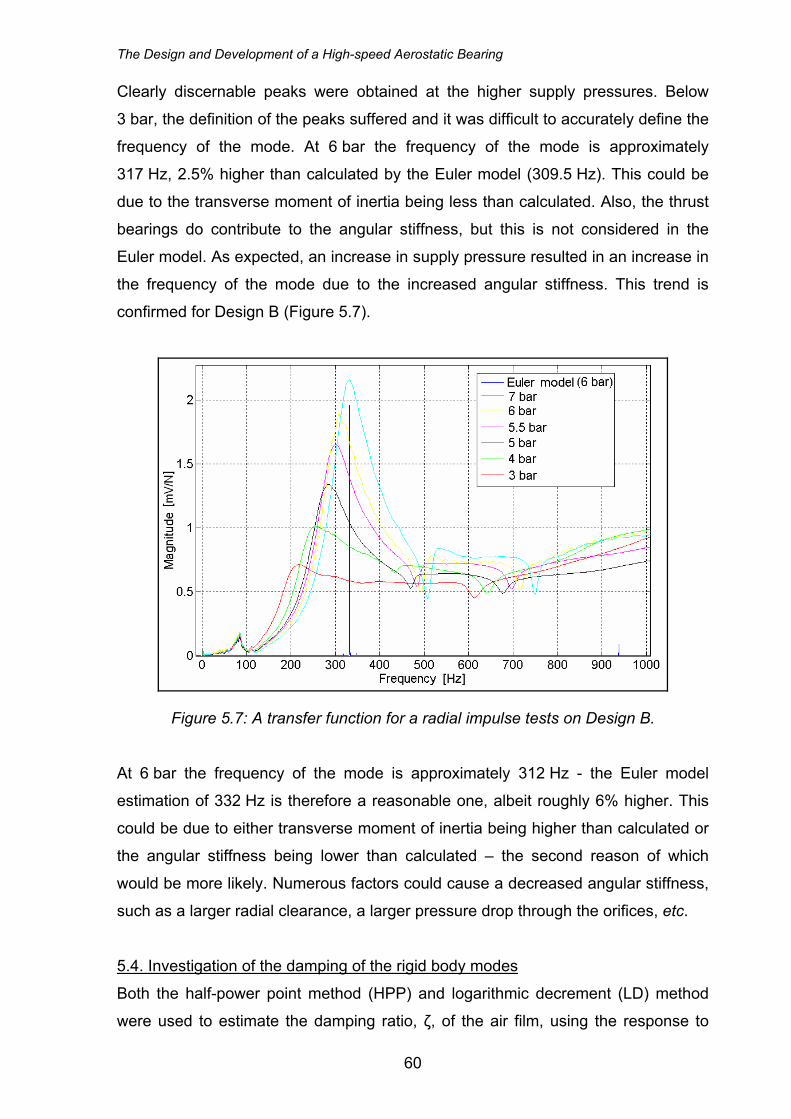
The Design and Development of a High-speed Aerostatic Bearing
Clearly discernable peaks were obtained at the higher supply pressures. Below
3 bar, the definition of the peaks suffered and it was difficult to accurately define the
frequency of the mode. At 6 bar the frequency of the mode is approximately
317 Hz, 2.5% higher than calculated by the Euler model (309.5 Hz). This could be
due to the transverse moment of inertia being less than calculated. Also, the thrust
bearings do contribute to the angular stiffness, but this is not considered in the
Euler model. As expected, an increase in supply pressure resulted in an increase in
the frequency of the mode due to the increased angular stiffness. This trend is
confirmed for Design B (Figure 5.7).
Figure 5.7: A transfer function for a radial impulse tests on Design B.
At 6 bar the frequency of the mode is approximately 312 Hz - the Euler model
estimation of 332 Hz is therefore a reasonable one, albeit roughly 6% higher. This
could be due to either transverse moment of inertia being higher than calculated or
the angular stiffness being lower than calculated – the second reason of which
would be more likely. Numerous factors could cause a decreased angular stiffness,
such as a larger radial clearance, a larger pressure drop through the orifices, etc.
5.4. Investigation of the damping of the rigid body modes
Both the half-power point method (HPP) and logarithmic decrement (LD) method
were used to estimate the damping ratio, ζ, of the air film, using the response to
60
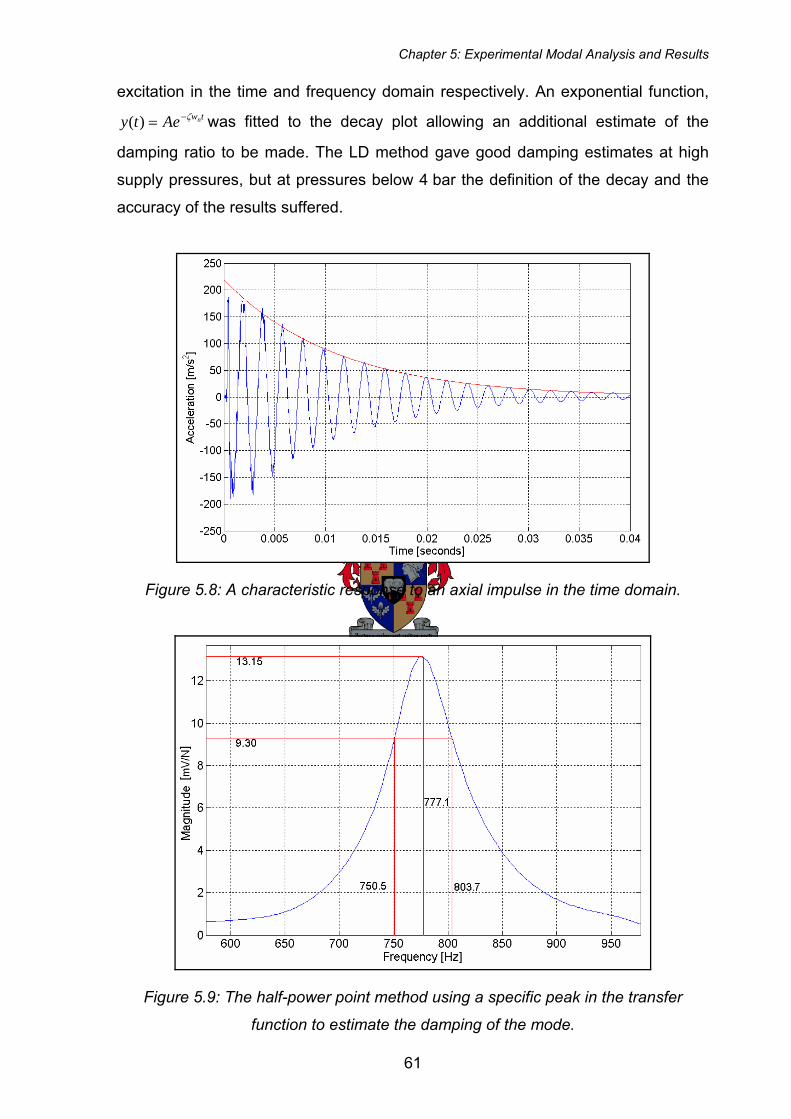
Chapter 5: Experimental Modal Analysis and Results
excitation in the time and frequency domain respectively. An exponential function,
was fitted to the decay plot allowing an additional estimate of the
damping ratio to be made. The LD method gave good damping estimates at high
supply pressures, but at pressures below 4 bar the definition of the decay and the
accuracy of the results suffered.
twnAety ζ−=)(
Figure 5.8: A characteristic response to an axial impulse in the time domain.
Figure 5.9: The half-power point method using a specific peak in the transfer
function to estimate the damping of the mode.
61
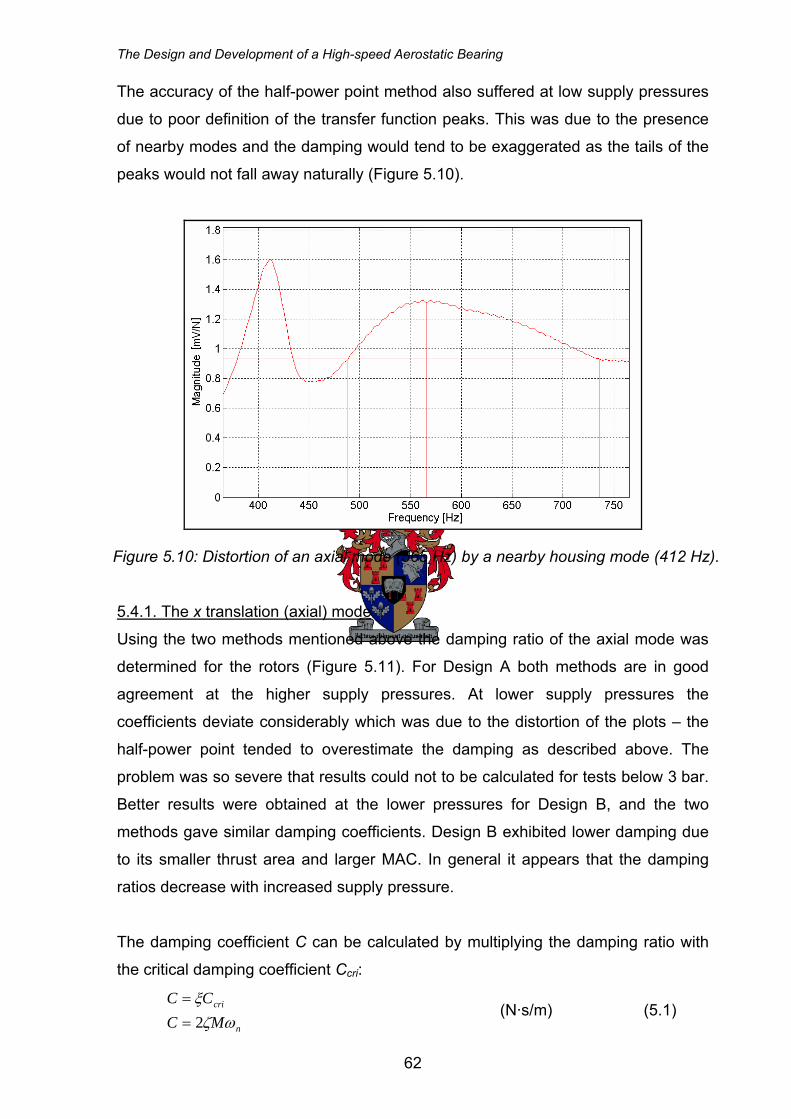
The Design and Development of a High-speed Aerostatic Bearing
The accuracy of the half-power point method also suffered at low supply pressures
due to poor definition of the transfer function peaks. This was due to the presence
of nearby modes and the damping would tend to be exaggerated as the tails of the
peaks would not fall away naturally (Figure 5.10).
Figure 5.10: Distortion of an axial mode (565 Hz) by a nearby housing mode (412 Hz).
5.4.1. The x translation (axial) mode
Using the two methods mentioned above the damping ratio of the axial mode was
determined for the rotors (Figure 5.11). For Design A both methods are in good
agreement at the higher supply pressures. At lower supply pressures the
coefficients deviate considerably which was due to the distortion of the plots – the
half-power point tended to overestimate the damping as described above. The
problem was so severe that results could not to be calculated for tests below 3 bar.
Better results were obtained at the lower pressures for Design B, and the two
methods gave similar damping coefficients. Design B exhibited lower damping due
to its smaller thrust area and larger MAC. In general it appears that the damping
ratios decrease with increased supply pressure.
The damping coefficient C can be calculated by multiplying the damping ratio with
the critical damping coefficient Ccri:
n
cri
MCCC
ωζξ2=
= (N·s/m) (5.1)
62
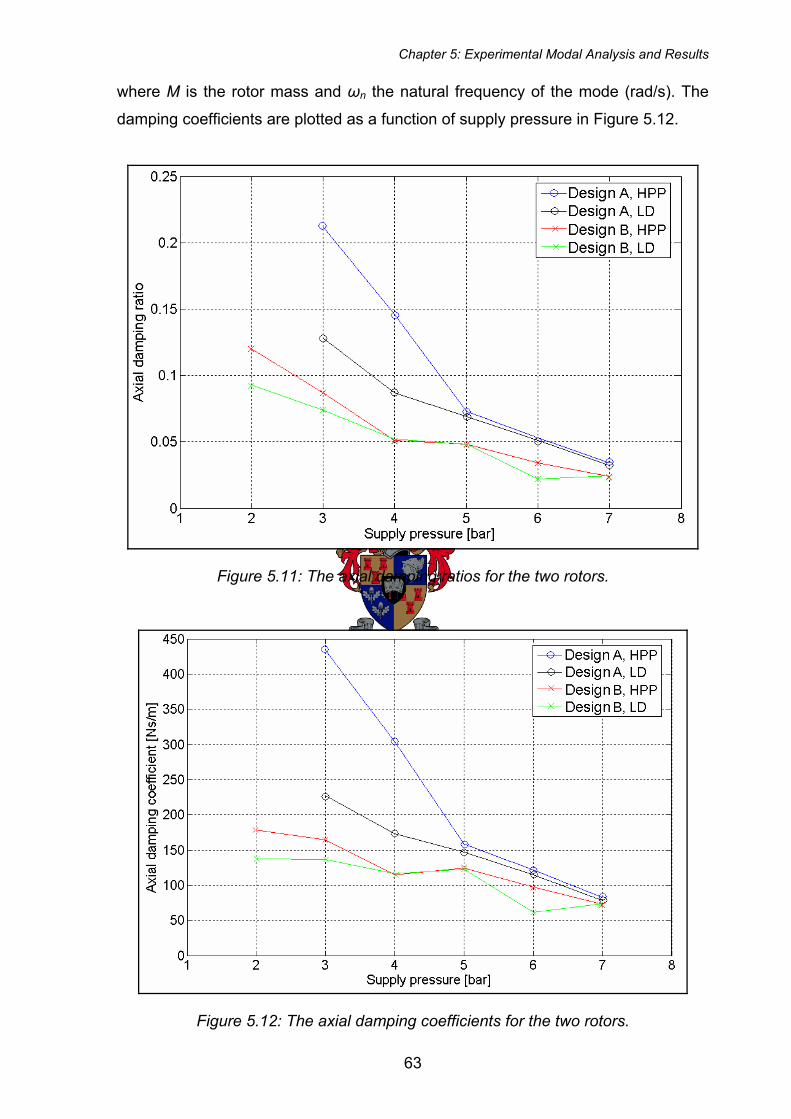
Chapter 5: Experimental Modal Analysis and Results
where M is the rotor mass and ωn the natural frequency of the mode (rad/s). The
damping coefficients are plotted as a function of supply pressure in Figure 5.12.
Figure 5.11: The axial damping ratios for the two rotors.
Figure 5.12: The axial damping coefficients for the two rotors.
63
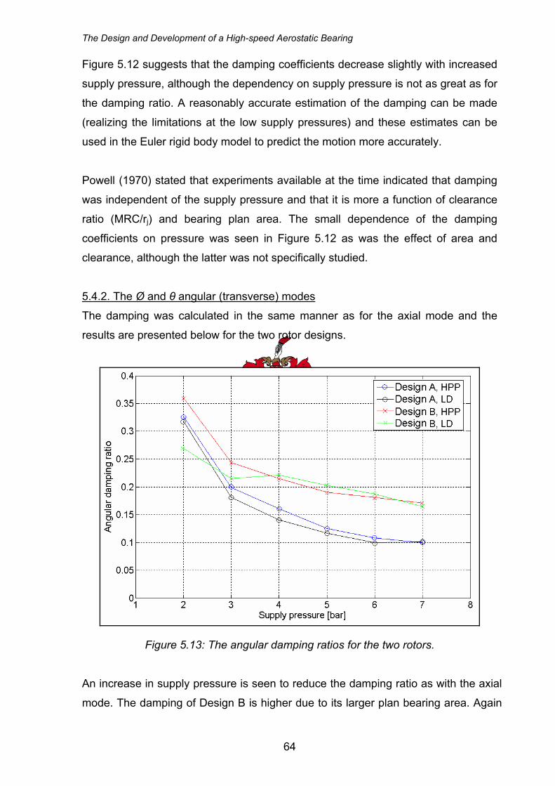
The Design and Development of a High-speed Aerostatic Bearing
Figure 5.12 suggests that the damping coefficients decrease slightly with increased
supply pressure, although the dependency on supply pressure is not as great as for
the damping ratio. A reasonably accurate estimation of the damping can be made
(realizing the limitations at the low supply pressures) and these estimates can be
used in the Euler rigid body model to predict the motion more accurately.
Powell (1970) stated that experiments available at the time indicated that damping
was independent of the supply pressure and that it is more a function of clearance
ratio (MRC/rj) and bearing plan area. The small dependence of the damping
coefficients on pressure was seen in Figure 5.12 as was the effect of area and
clearance, although the latter was not specifically studied.
5.4.2. The Ø and θ angular (transverse) modes
The damping was calculated in the same manner as for the axial mode and the
results are presented below for the two rotor designs.
Figure 5.13: The angular damping ratios for the two rotors.
An increase in supply pressure is seen to reduce the damping ratio as with the axial
mode. The damping of Design B is higher due to its larger plan bearing area. Again
64
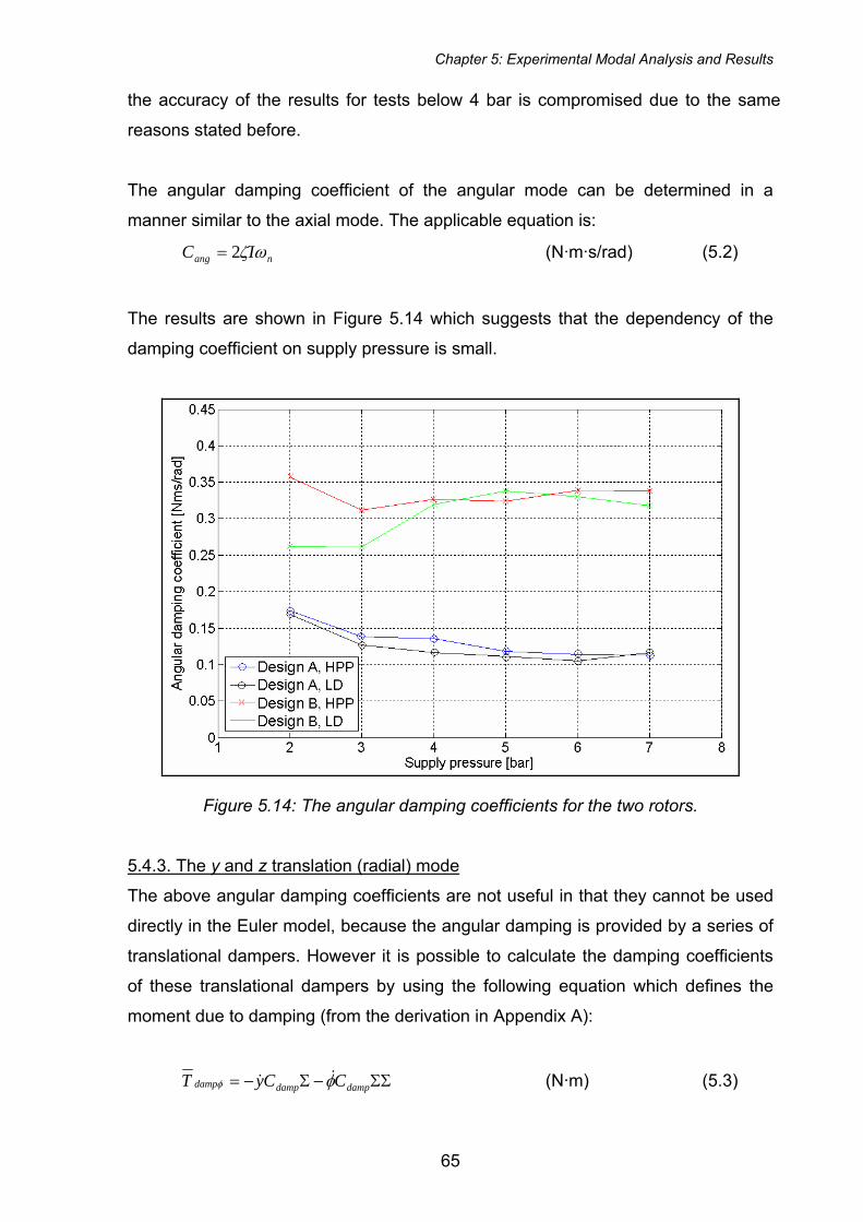
Chapter 5: Experimental Modal Analysis and Results
the accuracy of the results for tests below 4 bar is compromised due to the same
reasons stated before.
The angular damping coefficient of the angular mode can be determined in a
manner similar to the axial mode. The applicable equation is:
nang IC ωζ2= (N·m·s/rad) (5.2)
The results are shown in Figure 5.14 which suggests that the dependency of the
damping coefficient on supply pressure is small.
Figure 5.14: The angular damping coefficients for the two rotors.
5.4.3. The y and z translation (radial) mode
The above angular damping coefficients are not useful in that they cannot be used
directly in the Euler model, because the angular damping is provided by a series of
translational dampers. However it is possible to calculate the damping coefficients
of these translational dampers by using the following equation which defines the
moment due to damping (from the derivation in Appendix A):
ΣΣ−Σ−= dampdampdamp CCyT φφ && (N·m) (5.3)
65
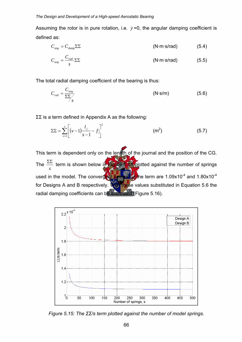
The Design and Development of a High-speed Aerostatic Bearing
Assuming the rotor is in pure rotation, i.e. =0, the angular damping coefficient is
defined as:
y&
(N·m·s/rad) (5.4) ΣΣ= dampang CC
ΣΣ=s
CC rad
ang (N·m·s/rad) (5.5)
The total radial damping coefficient of the bearing is thus:
s
CC ang
rad ΣΣ= (N·s/m) (5.6)
ΣΣ is a term defined in Appendix A as the following:
( )2
1 11∑
=⎥⎦
⎤⎢⎣
⎡−
−−=ΣΣ
s
v
j fsl
v (m2) (5.7)
This term is dependent only on the length of the journal and the position of the CG.
The sΣΣ term is shown below in Figure 5.15 plotted against the number of springs
used in the model. The convergent values for the term are 1.09x10⁻⁴ and 1.80x10⁻⁴
for Designs A and B respectively. With these values substituted in Equation 5.6 the
radial damping coefficients can be estimated (Figure 5.16).
Figure 5.15: The ΣΣ/s term plotted against the number of model springs.
66
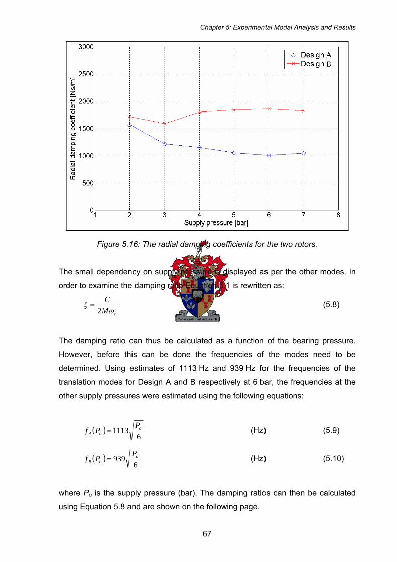
Chapter 5: Experimental Modal Analysis and Results
Figure 5.16: The radial damping coefficients for the two rotors.
The small dependency on supply pressure is displayed as per the other modes. In
order to examine the damping ratio Equation 5.1 is rewritten as:
nM
Cω
ξ2
= (5.8)
The damping ratio can thus be calculated as a function of the bearing pressure.
However, before this can be done the frequencies of the modes need to be
determined. Using estimates of 1113 Hz and 939 Hz for the frequencies of the
translation modes for Design A and B respectively at 6 bar, the frequencies at the
other supply pressures were estimated using the following equations:
( )6
1113 ooA
PPf = (Hz) (5.9)
( )6
939 ooB
PPf = (Hz) (5.10)
where Po is the supply pressure (bar). The damping ratios can then be calculated
using Equation 5.8 and are shown on the following page.
67
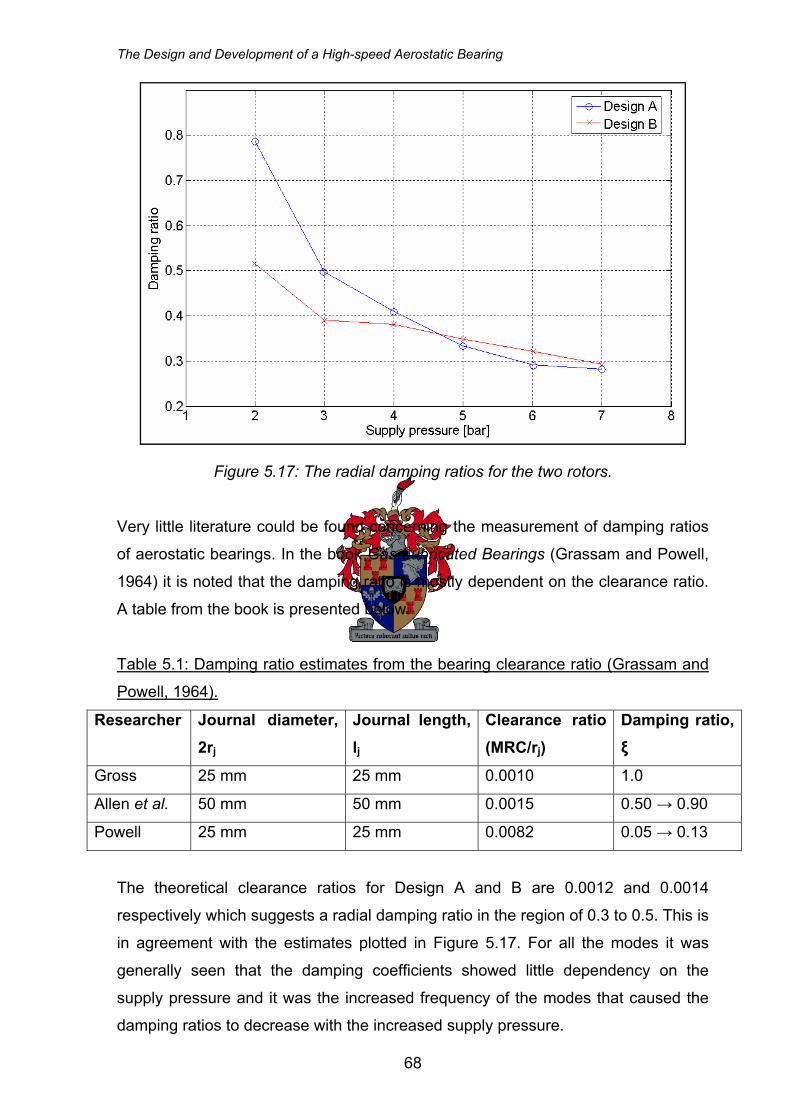
The Design and Development of a High-speed Aerostatic Bearing
Figure 5.17: The radial damping ratios for the two rotors.
Very little literature could be found concerning the measurement of damping ratios
of aerostatic bearings. In the book Gas Lubricated Bearings (Grassam and Powell,
1964) it is noted that the damping ratio is mostly dependent on the clearance ratio.
A table from the book is presented below.
Table 5.1: Damping ratio estimates from the bearing clearance ratio (Grassam and
Powell, 1964).
Researcher Journal diameter, 2rj
Journal length, lj
Clearance ratio (MRC/rj)
Damping ratio, ξ
Gross 25 mm 25 mm 0.0010 1.0
Allen et al. 50 mm 50 mm 0.0015 0.50 → 0.90
Powell 25 mm 25 mm 0.0082 0.05 → 0.13
The theoretical clearance ratios for Design A and B are 0.0012 and 0.0014
respectively which suggests a radial damping ratio in the region of 0.3 to 0.5. This is
in agreement with the estimates plotted in Figure 5.17. For all the modes it was
generally seen that the damping coefficients showed little dependency on the
supply pressure and it was the increased frequency of the modes that caused the
damping ratios to decrease with the increased supply pressure.
68
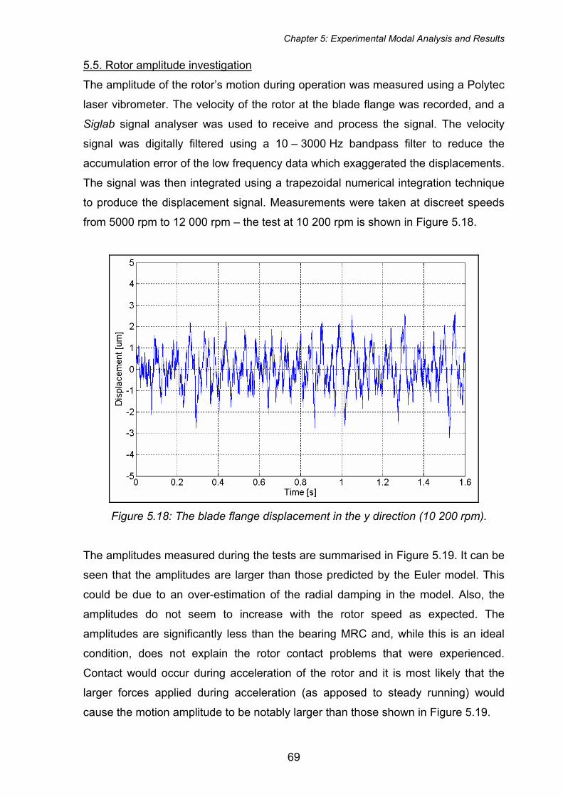
Chapter 5: Experimental Modal Analysis and Results
5.5. Rotor amplitude investigation
The amplitude of the rotor’s motion during operation was measured using a Polytec
laser vibrometer. The velocity of the rotor at the blade flange was recorded, and a
Siglab signal analyser was used to receive and process the signal. The velocity
signal was digitally filtered using a 10 – 3000 Hz bandpass filter to reduce the
accumulation error of the low frequency data which exaggerated the displacements.
The signal was then integrated using a trapezoidal numerical integration technique
to produce the displacement signal. Measurements were taken at discreet speeds
from 5000 rpm to 12 000 rpm – the test at 10 200 rpm is shown in Figure 5.18.
Figure 5.18: The blade flange displacement in the y direction (10 200 rpm).
The amplitudes measured during the tests are summarised in Figure 5.19. It can be
seen that the amplitudes are larger than those predicted by the Euler model. This
could be due to an over-estimation of the radial damping in the model. Also, the
amplitudes do not seem to increase with the rotor speed as expected. The
amplitudes are significantly less than the bearing MRC and, while this is an ideal
condition, does not explain the rotor contact problems that were experienced.
Contact would occur during acceleration of the rotor and it is most likely that the
larger forces applied during acceleration (as apposed to steady running) would
cause the motion amplitude to be notably larger than those shown in Figure 5.19.
69
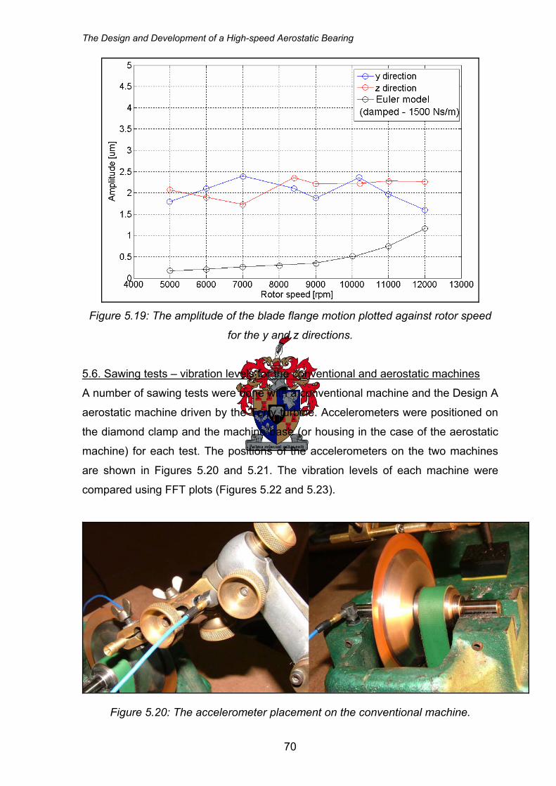
The Design and Development of a High-speed Aerostatic Bearing
Figure 5.19: The amplitude of the blade flange motion plotted against rotor speed
for the y and z directions.
5.6. Sawing tests – vibration levels for the conventional and aerostatic machines
A number of sawing tests were done with a conventional machine and the Design A
aerostatic machine driven by the Terry turbine. Accelerometers were positioned on
the diamond clamp and the machine base (or housing in the case of the aerostatic
machine) for each test. The positions of the accelerometers on the two machines
are shown in Figures 5.20 and 5.21. The vibration levels of each machine were
compared using FFT plots (Figures 5.22 and 5.23).
Figure 5.20: The accelerometer placement on the conventional machine.
70
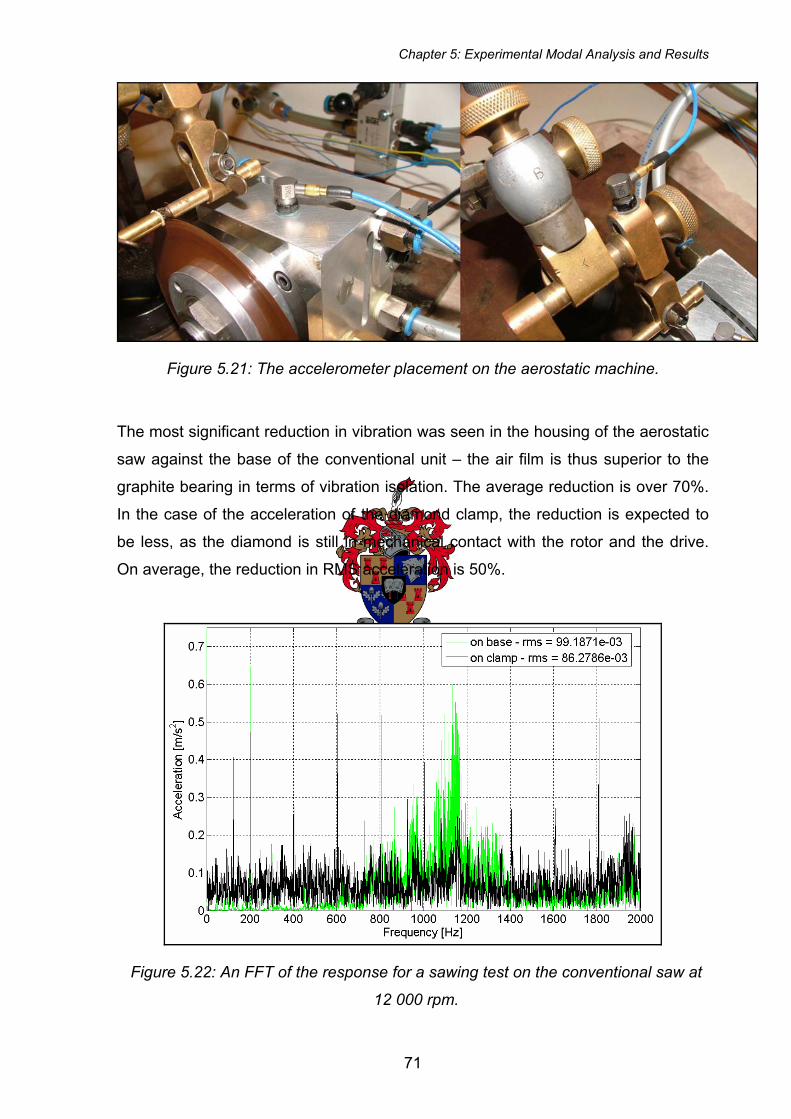
Chapter 5: Experimental Modal Analysis and Results
Figure 5.21: The accelerometer placement on the aerostatic machine.
The most significant reduction in vibration was seen in the housing of the aerostatic
saw against the base of the conventional unit – the air film is thus superior to the
graphite bearing in terms of vibration isolation. The average reduction is over 70%.
In the case of the acceleration of the diamond clamp, the reduction is expected to
be less, as the diamond is still in mechanical contact with the rotor and the drive.
On average, the reduction in RMS acceleration is 50%.
Figure 5.22: An FFT of the response for a sawing test on the conventional saw at
12 000 rpm.
71
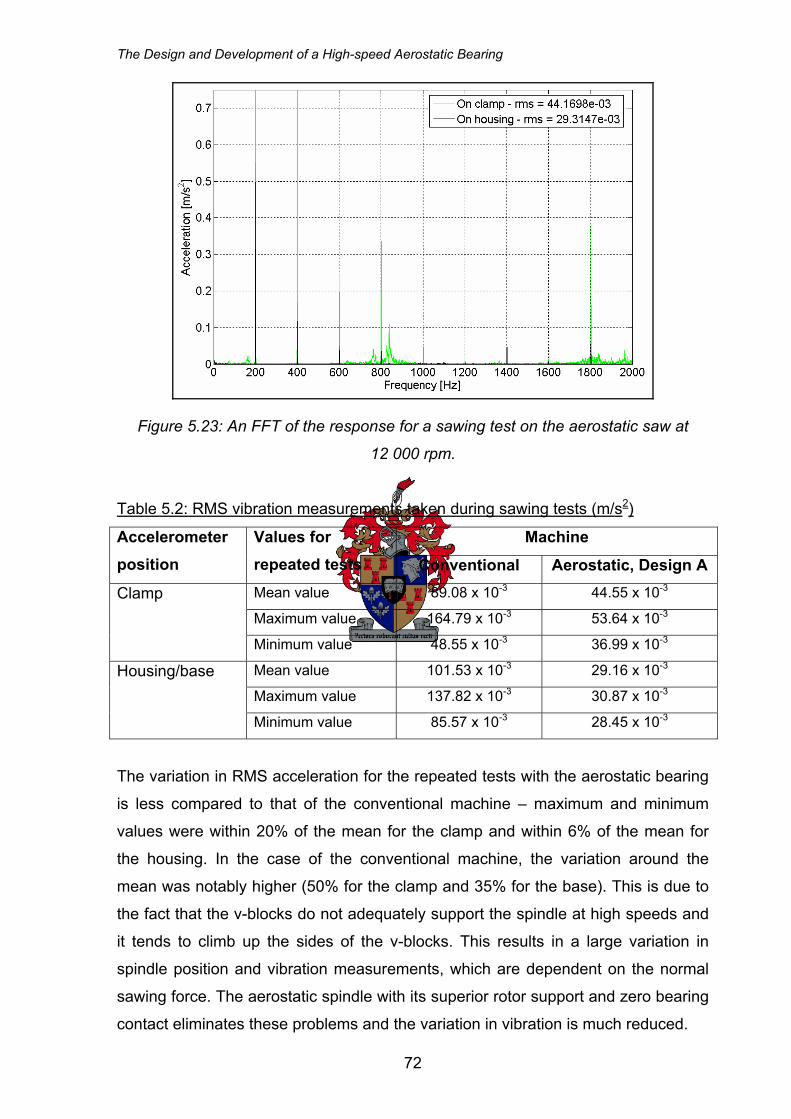
The Design and Development of a High-speed Aerostatic Bearing
Figure 5.23: An FFT of the response for a sawing test on the aerostatic saw at
12 000 rpm.
Table 5.2: RMS vibration measurements taken during sawing tests (m/s2)
Machine Accelerometer position
Values for repeated tests Conventional Aerostatic, Design A Mean value 89.08 x 10⁻³ 44.55 x 10⁻³
Maximum value 164.79 x 10⁻³ 53.64 x 10⁻³
Clamp
Minimum value 48.55 x 10⁻³ 36.99 x 10⁻³
Mean value 101.53 x 10⁻³ 29.16 x 10⁻³
Maximum value 137.82 x 10⁻³ 30.87 x 10⁻³
Housing/base
Minimum value 85.57 x 10⁻³ 28.45 x 10⁻³
The variation in RMS acceleration for the repeated tests with the aerostatic bearing
is less compared to that of the conventional machine – maximum and minimum
values were within 20% of the mean for the clamp and within 6% of the mean for
the housing. In the case of the conventional machine, the variation around the
mean was notably higher (50% for the clamp and 35% for the base). This is due to
the fact that the v-blocks do not adequately support the spindle at high speeds and
it tends to climb up the sides of the v-blocks. This results in a large variation in
spindle position and vibration measurements, which are dependent on the normal
sawing force. The aerostatic spindle with its superior rotor support and zero bearing
contact eliminates these problems and the variation in vibration is much reduced.
72
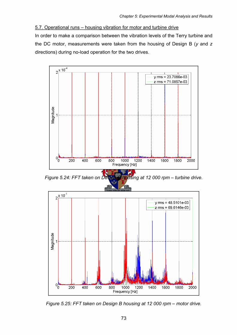
Chapter 5: Experimental Modal Analysis and Results
5.7. Operational runs – housing vibration for motor and turbine drive
In order to make a comparison between the vibration levels of the Terry turbine and
the DC motor, measurements were taken from the housing of Design B (y and z
directions) during no-load operation for the two drives.
Figure 5.24: FFT taken on Design B housing at 12 000 rpm – turbine drive.
Figure 5.25: FFT taken on Design B housing at 12 000 rpm – motor drive.
73
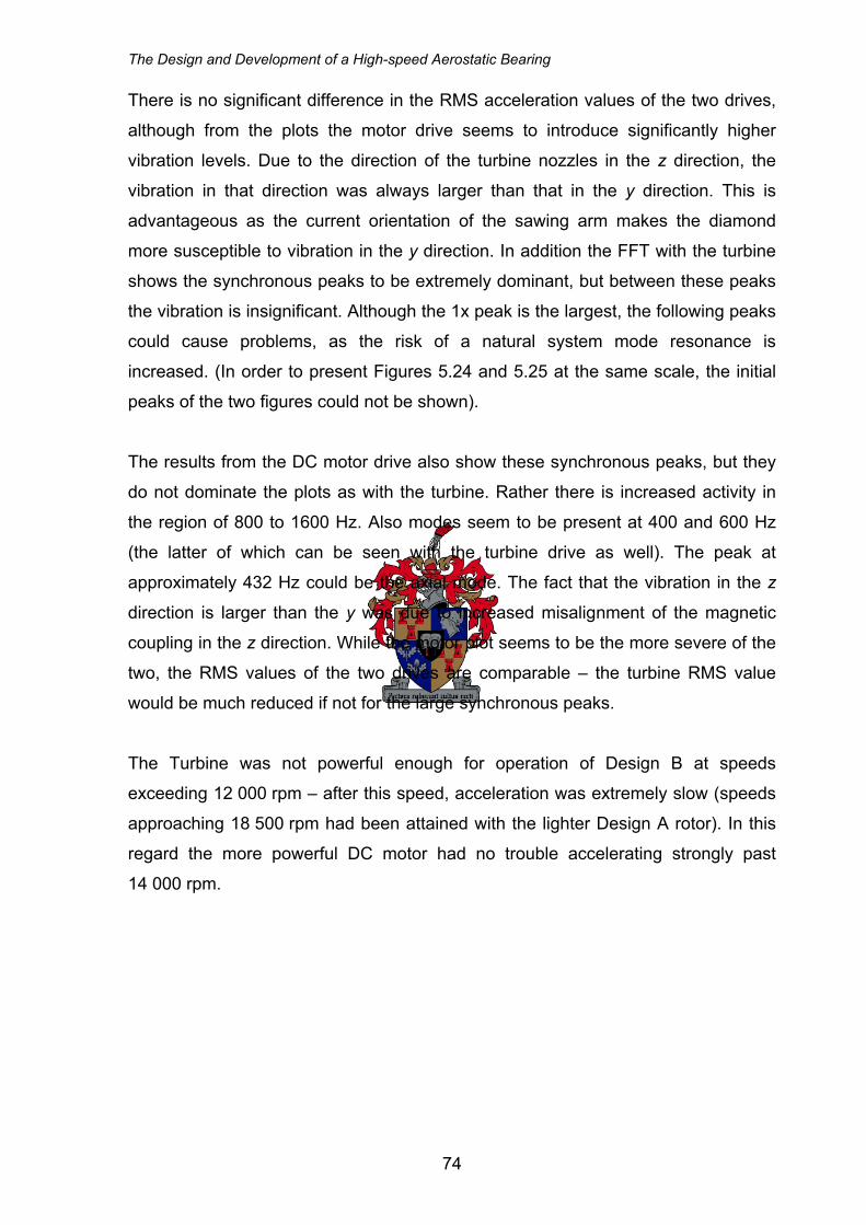
The Design and Development of a High-speed Aerostatic Bearing
There is no significant difference in the RMS acceleration values of the two drives,
although from the plots the motor drive seems to introduce significantly higher
vibration levels. Due to the direction of the turbine nozzles in the z direction, the
vibration in that direction was always larger than that in the y direction. This is
advantageous as the current orientation of the sawing arm makes the diamond
more susceptible to vibration in the y direction. In addition the FFT with the turbine
shows the synchronous peaks to be extremely dominant, but between these peaks
the vibration is insignificant. Although the 1x peak is the largest, the following peaks
could cause problems, as the risk of a natural system mode resonance is
increased. (In order to present Figures 5.24 and 5.25 at the same scale, the initial
peaks of the two figures could not be shown).
The results from the DC motor drive also show these synchronous peaks, but they
do not dominate the plots as with the turbine. Rather there is increased activity in
the region of 800 to 1600 Hz. Also modes seem to be present at 400 and 600 Hz
(the latter of which can be seen with the turbine drive as well). The peak at
approximately 432 Hz could be the axial mode. The fact that the vibration in the z
direction is larger than the y was due to increased misalignment of the magnetic
coupling in the z direction. While the motor plot seems to be the more severe of the
two, the RMS values of the two drives are comparable – the turbine RMS value
would be much reduced if not for the large synchronous peaks.
The Turbine was not powerful enough for operation of Design B at speeds
exceeding 12 000 rpm – after this speed, acceleration was extremely slow (speeds
approaching 18 500 rpm had been attained with the lighter Design A rotor). In this
regard the more powerful DC motor had no trouble accelerating strongly past
14 000 rpm.
74
Chapter 6: Conclusions and Recommendations
The implementation of an aerostatic bearing in the diamond sawing machine was
successful in reducing vibration at both the housing (by 70%) and the diamond
clamp (by 50%), while at the same time making significantly higher spindle speeds
possible – 18 500 rpm was achieved by Design A. In terms of the reduced vibration
and increased speed requirements it was the most appropriate bearing type for the
application. This chapter includes the concluded remarks on the project and
provides further recommendations.
6.1. The FEM analysis, Euler rigid body model and EMA
FEM analysis was used to verify the validity of assuming the rotor to be rigid. EMA
confirmed the theoretical results to within 6%. A rigid body model was developed
using the modified Euler equations of motion in order to predict the natural
frequencies of the rotor system as well as the amplitude of the rotor motion. The
natural frequencies of the rotor’s vibration modes can be calculated with sufficient
accuracy by using SDOF vibration theory. This excludes the two angular vibration
modes which, due to gyroscopic forces, are dependent on the rotor speed. This
bifurcation is similar to that observed with the forwards and backwards whirling of
flexible shafts. The EMA was successful in determining the experimental
frequencies and damping of the rigid body modes. The frequencies of the natural
modes were predicted reasonably accurately by the Euler model with the maximum
error of 6%. The bearing stiffness (and thus mode frequency) was seen to be
strongly dependent on the clearance. There was not sufficient theory available to
gauge the accuracy of the damping results obtained. The results indicated that the
damping coefficients were not strongly dependent on supply pressure, but because
the frequency of the modes increased with pressure the damping ratios tended to
decrease with increased pressure. The bearing clearance was seen to have a
larger effect although this was not specifically studied.
The accuracy of the amplitude prediction was not as good as that of the
frequencies. This was mainly due to the uncertainty in the radial damping of the
bearing. The laser vibrometer test results indicated that the amplitude of the rotor
motion was well within the clearance of the bearing, yet rotor contact was a serious,
75
The Design and Development of a High-speed Aerostatic Bearing
persistent problem during test sessions. The maximum speed obtained by Design A
was 18 500 rpm and 15 000 rpm for Design B. This is less than the desired speed
of the machine and thus this aspect of the design requires further attention. No
specific rotor modes were observed during vibration measurement of a running
rotor, neither on the housing nor on the rotors, which is highly desirable in terms of
reduced vibration. This could be due to the fact that the rotor could not be run at
speeds that could excite these modes sufficiently.
6.2. An improved bearing and rotor design – Design C
Based on the comparison with the experimental results and the Euler model, an
improved design, Design C, was completed - it is described in this section.
The use of a single, central journal bearing with two exhaust-fed thrust bearings on
either end was a suitable design choice. It simplified manufacture and minimised air
consumption while providing sufficient axial support of the rotor. It can be added
that if a magnetic coupling is used, only a single thrust face would be required as
the tension of the coupling would support the rotor axially. This would eliminate the
extra components and extra set-up time concerned with an additional thrust face.
Design C would utilise a quarter-station design in order to increase the angular
stiffness. For the same reason simple jets will be used, with the added advantage
that they can be replaced if they become blocked. In order to solve the contact
problems the angular stiffness of the new bearing has been increased by over
100%, mainly due to an increase in the journal dimensions and a reduction in the
MRC. These specifications were achieved in spite of a reduced design pressure of
4 bar. The decrease in clearance was motivated by the following bearing design
characteristics (Slocum, 1994; Wilcock, 1957; Stansfield, 1970):
MRCStiffness 1
∝ , 3
1MRC
Damping ∝ , Air 3MRCnconsumptio ∝
Thus the MRC should be made as small as practically possible, while ensuring that
the machinist responsible for the manufacture is able to finish the components to
within the correct tolerance reliably. The frequency of angular vibration had to be at
least 20% higher than the highest conceivable operating speed, which for Design C
76
Chapter 6: Conclusions and Recommendations
has been set at 25 000 rpm (417 Hz). Thus the frequency of the angular mode
needed to be more than 500 Hz. These stiffness specifications were designed at
4 bar to reduce air consumption, take advantage of the increased damping at the
lower pressure and allow a margin of safety (i.e. an increase in supply pressure) in
case the stiffness needs to be increased.
The best solution regarding material selection for the shaft is to use a hard-
anodised aluminium rotor and to incorporate a safety control system which brings
the rotor to rest if the supply pressure falls below a certain value. The reason for
this is that a hardened steel shaft was not seen to be significantly better than the
hard-anodised aluminium in terms of resistance to contact, and it was clearly
inferior in terms of rotor mass which needs to be minimised. This route would result
in the smallest and lightest rotor, which in turn would reduce manufacturing costs.
The use of stainless-steel and brass for the bearing-bush and feed jets respectively
will be retained. The thrust faces will be hard-anodised aluminium to reduce weight.
One thrust face will be integral with the shaft to eliminate the set up effort during
assembly. Contrary to Design A, the integral face will be on the blade flange side,
rather on the drive side, to improve the support of the blade and ensure its
perpendicular requirement is as accurate as possible. The other thrust face needs
to be secured to the shaft in such a way that it is not pulled skew from the axis
when tightened. Using a threaded connection is not acceptable and a ball-and-
socket or similar concept would be far better. The MAC has been increased to ease
assembly. The reduction in axial stiffness will have no adverse effect on the rotor in
the application but its effect on the axial vibration frequency was taken into account.
The specifications of the new bearing at 4 bar are as follows:
• Journal diameter, 30 mm
• Journal length, 60 mm
• Thrust bearing diameter, 60 mm
• Mean radial clearance, 15 μm
• Mean axial clearance, 30 μm
• Rotor mass, 350 g
• Polar moment of inertia, 100 kg·m2
77
The Design and Development of a High-speed Aerostatic Bearing
• Transverse moment of inertia, 370 kg·m2
• Radial stiffness, 20 MN/m
• Angular stiffness, 4555 N·m/rad
The theoretical frequencies of the system modes estimated by the Euler model at
25 000 rpm are:
• Axial mode, 535 Hz
• Phi angular mode, 505 Hz
• Theta angular mode, 617.5 Hz
• Radial translation, 1207 Hz
With the vibration of the two drives being comparable, the decision of which one to
use becomes more economical in nature. The current Terry turbine is not powerful
enough for operation at the desired speeds and so the economic factors of a more
powerful turbine versus the DC motor must be weighed up. It can be added that a
radial inflow turbine of the required power output might be superior to the Terry
turbine. The many synchronous peaks observed in the vibration data could be
eliminated by the absence of the pockets in the radial turbine. If so, this turbine
would achieve lower vibration than the DC motor and would be a better choice.
However, the air consumption of the turbine would have to be compared with the
cost of the DC motor controller and power supply before a decision can be made.
The air consumption of the Terry-type turbine was in the region of 100 l/m at
14 000 rpm with zero load on the blade (driving the Design A rotor).
In order to increase the stability of the rotor at speed, two additional design routes
may be visited. One would be the investigation of a porous compensated bush in
place of the jet compensation. It is stated in the literature (New Way Precision,
2003) that porous compensation creates a more uniform pressure distribution along
the journal length as well as increases the damping of the system. It is also more
resistant to rotor contact (especially if a self-lubricating material such as sintered
carbon is used) and has a lower Q value to improve the angular stiffness. If this
route is investigated, a study of the permeability of the bushes would be required in
order to achieve the correct compensation for the bearing.
78
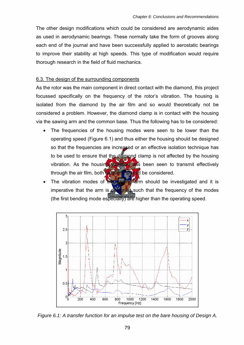
Chapter 6: Conclusions and Recommendations
The other design modifications which could be considered are aerodynamic aides
as used in aerodynamic bearings. These normally take the form of grooves along
each end of the journal and have been successfully applied to aerostatic bearings
to improve their stability at high speeds. This type of modification would require
thorough research in the field of fluid mechanics.
6.3. The design of the surrounding components
As the rotor was the main component in direct contact with the diamond, this project
focussed specifically on the frequency of the rotor’s vibration. The housing is
isolated from the diamond by the air film and so would theoretically not be
considered a problem. However, the diamond clamp is in contact with the housing
via the sawing arm and the common base. Thus the following has to be considered:
• The frequencies of the housing modes were seen to be lower than the
operating speed (Figure 6.1) and thus either the housing should be designed
so that the frequencies are increased or an effective isolation technique has
to be used to ensure that the diamond clamp is not affected by the housing
vibration. As the housing vibration has been seen to transmit effectively
through the air film, both solutions should be considered.
• The vibration modes of the sawing arm should be investigated and it is
imperative that the arm is designed such that the frequency of the modes
(the first bending mode especially) are higher than the operating speed.
Figure 6.1: A transfer function for an impulse test on the bare housing of Design A.
79
The Design and Development of a High-speed Aerostatic Bearing
6.4. The diamond sawing process
The current method of periodically lowering the diamond into the blade results in a
small percentage of the total sawing time being used for effective sawing. Most of
the time the diamond is not completely in contact with the blade and the risk of the
feed being too heavy is always present. The reason for the use of this arrangement
is that, with the very small normal feed force required (0.1 N to 0.5 N), a bearing of
very low friction is required at the saw arm pivot. Any stiction (stick-slip condition)
present in the bearing is detrimental to the control of the feed force and results in
erratic variation in the force. With this in mind, a new concept is proposed whereby
the correct feed force is applied during the entire sawing time. This would consist of
a sawing arm similar to the one used in the current machine, with a translating
mass that can be slid along its length. No threaded feeding rod would be used and
the feed force would be dependent only on the centre of gravity of the arm, which
itself depends on the position of the translating mass. The pivot point of the arm
would incorporate a bearing of very low friction (ideally an aerostatic unit) to ensure
that only the mass affects the feed force. The diamond would be lowered onto the
rotating blade and left until the cut is complete. Using an aerostatic unit would also
provide a measure of isolation against housing vibration.
6.5. Possible further investigation – EMA on rotating components
Additional investigation which would be extremely useful to the success of the
project involves EMA on the rotor while it is operation. This would allow the
examination of the frequencies and damping of the system modes as a function of
the rotor speed (Bucher and Ewins, 2001).
The bifurcation of the angular modes could potentially be the cause of resonance
problems as the frequency of the ‘backwards’ whirling mode would be lower than
expected. Thus an investigation to confirm this phenomenon would be
advantageous to the stability of the rotor.
The theory indicates that the damping of fluid film bearings is dependent on the
velocity of the bearing surface. Thus it is dependent on rotor speed, and greater
knowledge of the dependency would greatly improve the accuracy of the Euler
model and allow a more efficient design of the bearing system.
80
References
A.G. Abulrub, P.S. Keogh, M.N. Sahinkaya, C.R. Burrows, 2005, Effective Model
reduction for Magnetically Levitated Flexible Rotor including Contact Dynamics,
Proceedings of IDETC/CIE 2005 (DETC2005-84418), ASME 2005 International
Design Engineering Technical Conferences, and Computers and Information in
Engineering Conference (Long Beach, USA)
B.M. Antkowiak, F.C. Nelson, undated, Rotordynamic Modeling of an Actively
Controlled Magnetic Bearing Gas Turbine Engine, Based on the paper published in
the Proceedings of the 1997 International Gas Turbine and Aeroengine Congress
and Exposition, ASME
H. Baruh, 1999, Analytical Dynamics, McGraw-Hill International Editions,
Mechanical Engineering Series
G.V. Brown, A.F. Fascak, R.H. Jansen, T.P. Dever, K.P. Duffy, January 2006,
Stabilizing Gyroscopic Modes in Magnetic-Bearing-Supported Flywheels by using
Cross-Axis Proportional Gains, National Aeronautics and Space Administration
Glenn Research Centre, Prepared for the Guidance, Navigation and Control
Conference and Exhibit
I. Bucher, D.J. Ewins, 2001, Modal Analysis and Testing of Rotating Structures, The
Royal Society London A (2001) 359, 61-96
C. T. Crowe, D. F. Elger, J. A. Roberson, 2001, Engineering Fluid Mechanics, 7th
Edition, John Wiley & Sons, Inc
M. S. Darlow, 1989, Balancing of High-Speed Machinery, Mechanical Engineering
Series, Springer-Verlag, New York
M.I. Friswell, J.E.T. Penny, S.D. Garvey, A.W. Lees, 2001, Damping Ratio and
Natural Frequency Bifurcations in Rotating Systems, Journal of Sound and
Vibration (2001) 245(5), 960-967
81
Design and Development of a High-speed Aerostatic Bearing
N.S. Grassam, J.W. Powell, 1964, Gas Lubricated Bearings, Butterworth & Co˙,
London
R.K. Harker, 1983, Generalized Methods of Vibration Analysis, University of
Wisconsin, Madison, John Wiley & Sons Inc., New York
J.P. Hartog, Mechanical Vibrations, Massachusetts Institute of Technology,
McGraw-Hill, New York, 1956
D. J. Inman, 2001, Engineering Vibration, 2nd Edition, Prentice Hall International
J.P. Khatait, W. Lin, W.J. Lin, 2005, Design and Development of an Orifice-Type
Aerostatic Thrust Bearing, SIMTech technical reports, Volume 6, Number 1
New Way Precision Bearings, 2003, Air Bearing Design and Application Guide,
Revision D, accessed July 2006
www.newwayairbearings.com
J.C. Nicholas, J.K. Whalen, S.D. Franklin, undated, Improving Critical Speed
Calculations using Flexible Bearing Support FRF Compliance Data, Dresser-Rand
Co.
J. Piers, D. Reynaerts, F. Verplaetsen, 2003, A Micro-Turbine for Electric Power
generation, Journal of Sensors and Actuators A: Physical (Elsevier) 113 (2004) 86-
93
J. Piers, D. Reynaerts, F. Verplaetsen, 2003, Development of an axial microturbine
for a portable gas turbine generator, Journal of Micromechanics and
Microengineering, 13 (2003) S190-S195
J. Piers, P. Vleugels, T. Waumans, M. Verlinden, D. Reynaerts, F. Verplaetsen,
2004, Development of High-Speed Bearings for Micro Gas Turbines,
MicroMechanics Europe Workshop
82
References
E.S. Piekos, K.S. Breuer, 2000, Manufacturing Effects in Microfabricated Gas
Bearings: Axially Varying Clearance, Journal of Tribology, Volume 124, October
2002
J.W. Powell, 1970, Design of Aerostatic Bearings, The Machinery Publishing
Company Ltd., Brighton
N. Savoulides, K.S. Breuer, S.A. Jacobson, F.F. Ehrich, 2000, Low Order Model for
Very Short Hybrid Gas Bearings, ASME, Tribology Division, Paper No. 2000-TRIB-
12
A. H. Slocum, 1994, Precision Machine Design, Topic 18: Externally Pressurised
Bearings
F.M. Stansfield, 1970, Hydrostatic Bearings, The Machinery Publishing Co˙ Ltd.,
Brighton
A. Surial, A. Kaushal, undated, Dynamic Analysis of Flexible Turbo-Rotor Systems
using Super-Elements
E. van Schalkwyk, 2006, Design and Control of a High Speed Rotor of a Diamond
Sawing Machine, Faculty of Mechanical Engineering, Stellenbosch University
B. Watermeyer, 1982, Diamond Cutting – 2nd Edition, Centaur Publishers
Johannesburg, South Africa
D.F. Wilcock, E.R. Booser, 1957, Bearing Design and Application, McGraw-Hill
Series in Mechanical Engineering, New York
E. Wilks, J. Wilks, 1994, Properties and Applications of Diamond
Butterworth-Heineman Ltd., Oxford
83

Design and Development of a High-speed Aerostatic Bearing
C.W. Wong, X. Zhang, S.A. Jacobson, A.H. Epstein, 2002, A Self-acting Thrust
Bearing for High Speed Micro-rotors, Journal of Microelectromechanical Systems
Volume 13, No˙ 2, April 2004
84

Bibliography
S. Zhou, J. Shi, 2001, Active Balancing and Vibration Control of Rotating
Machinery: A Survey, The Shock and Vibration Digest, Volume 33, No. 4
A.D. Dimarogonas, S.A. Paipetis, 1983, Analytical Methods in Rotor Dynamics,
Applied Science Publishers
Bently Pressurised Bearings, accessed June 2006
www.bentlypressurizedbearing.com
L. Meirovitch, 2001, Fundamentals of Vibrations, McGraw-Hill International Edition,
Mechanical Engineering Series
R.J. Harker, 1983, Generalized Methods of Vibration Analysis, John Wiley & Sons
Inc.
International Standard 20806, 2004, Mechanical vibration – Criteria and safeguards
for the in-situ balancing of medium and large rotors, International Organization for
Standardization (ISO)
V. Wowk, 1995, Machinery Vibration: Balancing, McGraw-Hill
P.P. Benham, R.J. Crawford, C.G. Armstrong, 1996, Mechanics of Engineering
Materials, 2nd Edition, Prentice Hall
P.S. Heyns, 1998, Mechanical Vibration – Measurement and Analysis, University of
Pretoria
H. Nakazawa, 1991, Principles of Precision Engineering, Oxford University Press
S. Zhou, J. Shi, undated, Supervisory Adaptive Balancing of Rigid Rotors during
Acceleration, University of Michigan
85
Design and Development of a High-speed Aerostatic Bearing
M.F. Dimentberg, 2005, Transverse Vibration of Rotating Shafts: Probability Density
and First-Passage Time of Whirl Radius, Journal of Non-linear Mechanics, 40
(2005) 1263-1267
O.E. Balje, 1981, Turbomachines – A Guide to Design, Selection and Theory, John
Wiley & Sons Inc., New York
C.W. de Silva, 2005, Vibration and Shock Handbook: Section I, Fundamentals and
Analysis, Chapter 3, Modal Analysis, Editor: C.W. de Silva, Taylor & Francis
C.W. de Silva, 2005, Vibration and Shock Handbook: Section I, Fundamentals and
Analysis, Chapter 18, Experimental Modal Analysis, Editor: C.W. de Silva, Taylor &
Francis
C.K. Mechefske, 2005, Vibration and Shock Handbook: Section I, Fundamentals
and Analysis, Chapter 25, Machine Condition Monitoring and Fault Diagnostics,
Editor: C.W. de Silver, Taylor & Francis
H.S. Samarasekera, 2005, Vibration and Shock Handbook: Section VIII, Design
and Applications, Chapter 34, Vibrations in Rotating Machinery, Editor: C.W. de
Silver, Taylor & Francis
M. Roseau, 1987, Vibrations in Mechanical Systems – Analytical Methods and
Applications, University of Paris VI – Pierre et Marie Curie, Springer-Verslag Berlin
Heidelberg
K. G. McConnell, 1995, Vibration Testing – Theory and Practice, Iowa State
University of Science and Technology, John Wiley & Sons, Inc
86
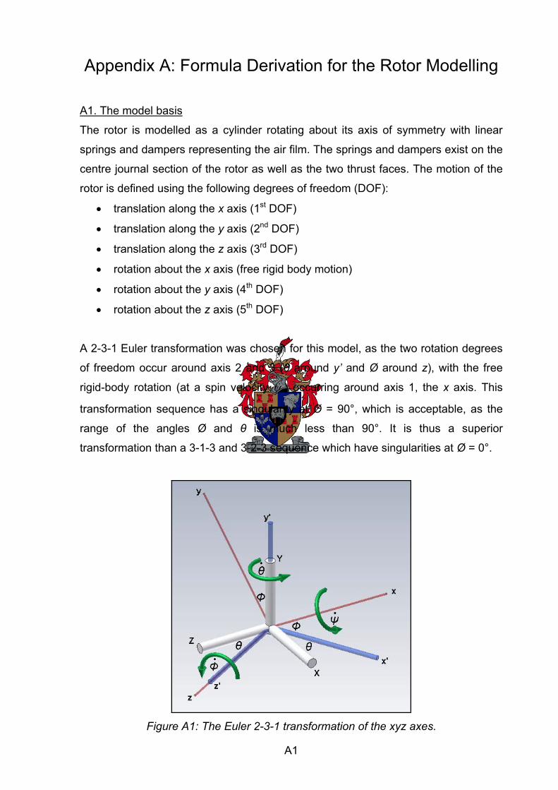
Appendix A: Formula Derivation for the Rotor Modelling
A1. The model basis
The rotor is modelled as a cylinder rotating about its axis of symmetry with linear
springs and dampers representing the air film. The springs and dampers exist on the
centre journal section of the rotor as well as the two thrust faces. The motion of the
rotor is defined using the following degrees of freedom (DOF):
• translation along the x axis (1st DOF)
• translation along the y axis (2nd DOF)
• translation along the z axis (3rd DOF)
• rotation about the x axis (free rigid body motion)
• rotation about the y axis (4th DOF)
• rotation about the z axis (5th DOF)
A 2-3-1 Euler transformation was chosen for this model, as the two rotation degrees
of freedom occur around axis 2 and 3 (θ around y’ and Ø around z), with the free
rigid-body rotation (at a spin velocity ψ& ) occurring around axis 1, the x axis. This
transformation sequence has a singularity at Ø = 90°, which is acceptable, as the
range of the angles Ø and θ is much less than 90°. It is thus a superior
transformation than a 3-1-3 and 3-2-3 sequence which have singularities at Ø = 0°.
Figure A1: The Euler 2-3-1 transformation of the xyz axes.
A1
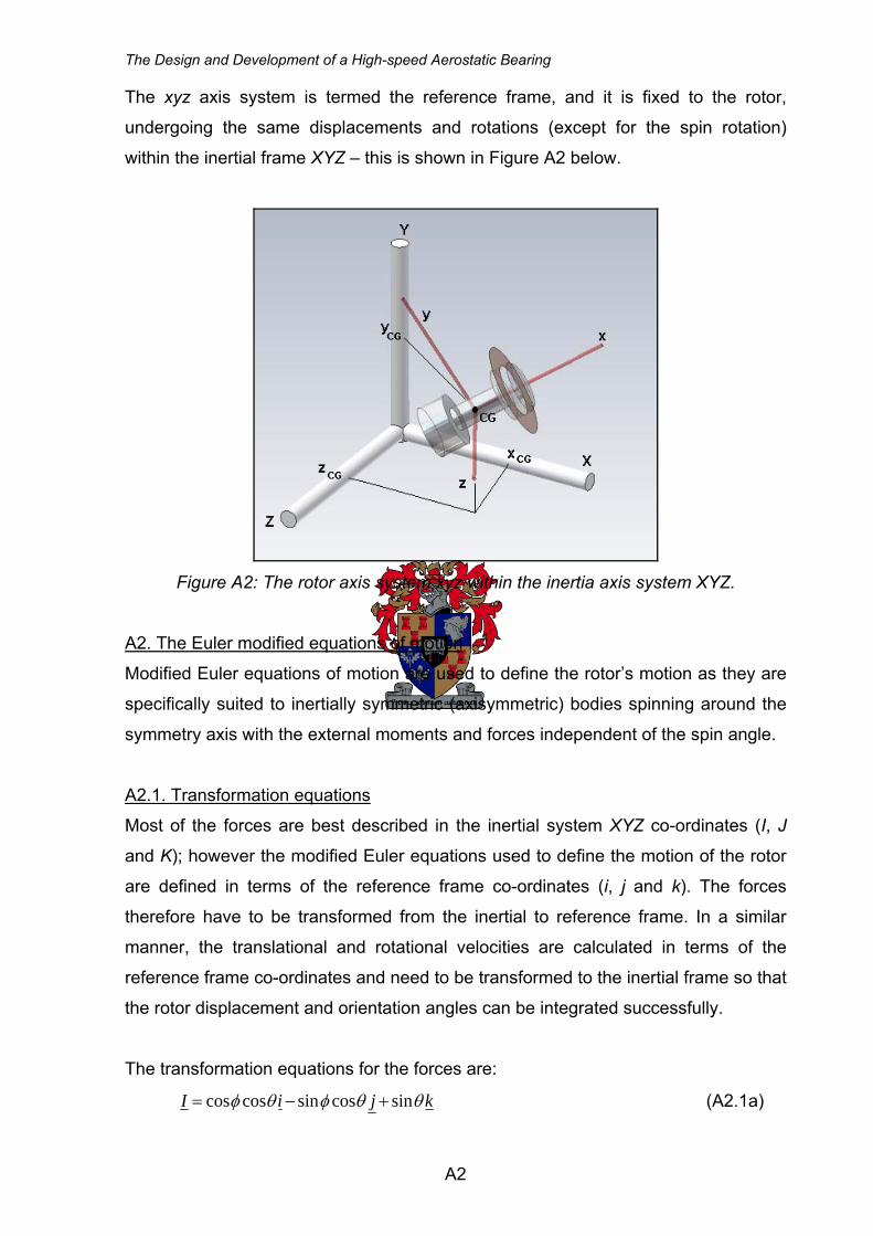
The Design and Development of a High-speed Aerostatic Bearing
The xyz axis system is termed the reference frame, and it is fixed to the rotor,
undergoing the same displacements and rotations (except for the spin rotation)
within the inertial frame XYZ – this is shown in Figure A2 below.
Figure A2: The rotor axis system xyz within the inertia axis system XYZ.
A2. The Euler modified equations of motion
Modified Euler equations of motion are used to define the rotor’s motion as they are
specifically suited to inertially symmetric (axisymmetric) bodies spinning around the
symmetry axis with the external moments and forces independent of the spin angle.
A2.1. Transformation equations
Most of the forces are best described in the inertial system XYZ co-ordinates (I, J
and K); however the modified Euler equations used to define the motion of the rotor
are defined in terms of the reference frame co-ordinates (i, j and k). The forces
therefore have to be transformed from the inertial to reference frame. In a similar
manner, the translational and rotational velocities are calculated in terms of the
reference frame co-ordinates and need to be transformed to the inertial frame so that
the rotor displacement and orientation angles can be integrated successfully.
The transformation equations for the forces are:
kjiI θθφθφ sincossincoscos +−= (A2.1a)
A2
Appendix A: Formula Derivation for the Rotor Modelling
jiJ φφ cossin += (A2.1b)
kjiK θφθφθ cossinsincossin ++−= (A2.1c)
The transformation equations for the body velocities are:
KJIi φθφφθ cossinsincoscos −+= (A2.2a)
KJIj φθφφθ sinsincossincos ++−= (A2.2b)
KIk θθ cossin += (A2.2c)
A2.2. The frame and body rotation velocities
The specific rotational velocities utilized in the Euler equations of motion are
described as follows:
Body spin rotational velocity, iBF
ψω &= (A2.3)
Frame rotational velocity, kji
jkFA
FA
φφθφθω
θφω
&&&
&&
++=
+=
cossin
' (A2.4)
Body rotational velocity, ( ) kji
BA
BFFABA
φφθψφθω
ωωω&&&& +++=
+=
cossin (A2.5)
A2.3. Euler’s modified rotational equations of motion
Euler’s modified equation of rotational motion is defined as:
{ } [ ]{ } [ ][ ]{ }ωωω GfrelGG IIM ~+= & (A2.6)
⎪⎭
⎪⎬
⎫
⎪⎩
⎪⎨
⎧
⎥⎥⎥
⎦
⎤
⎢⎢⎢
⎣
⎡
⎥⎥⎥
⎦
⎤
⎢⎢⎢
⎣
⎡
−−
−+
⎪⎭
⎪⎬
⎫
⎪⎩
⎪⎨
⎧
⎥⎥⎥
⎦
⎤
⎢⎢⎢
⎣
⎡=
⎪⎭
⎪⎬
⎫
⎪⎩
⎪⎨
⎧
3
2
1
12
13
23
3
2
1
000000
00
0
000000
ωωω
ωωωωωω
ωωω
zz
yy
xx
ff
ff
ff
zz
yy
xx
z
y
x
II
I
II
I
MMM
&
&
&
⎪⎭
⎪⎬
⎫
⎪⎩
⎪⎨
⎧
+−−++−
=⎪⎭
⎪⎬
⎫
⎪⎩
⎪⎨
⎧
21123
31132
32231
ωωωωωωωωωωωωωωω
yyfxxfzz
zzfxxfyy
zzfyyfxx
z
y
x
IIIIIIIII
MMM
&
&
&
(A2.7)
A3
The Design and Development of a High-speed Aerostatic Bearing
where the angular velocities for the reference frame and body are defined as
Body 1: (A2.8) ψφθω && += sin1
Frame 1: (A2.9) φωφθω tansin 21 == &f
Body and frame 2: (A2.10) φθωω cos22&== f
Body and frame 3: (A2.11) φωω &== 33 f
Using Equations A2.9 to A2.11, Equation A2.7 can be rewritten in terms of the body
angular velocities.
⎪⎭
⎪⎬
⎫
⎪⎩
⎪⎨
⎧
+−−++−
=⎪⎭
⎪⎬
⎫
⎪⎩
⎪⎨
⎧
22123
32132
32231
tantan
ωφωωωωωφωωωω
ωωωωω
yyxxzz
zzxxyy
zzyyxx
z
y
x
IIIIII
III
MMM
&
&
&
In this case Iyy = Izz, so further simplifications is possible
(( )⎪⎭
⎪⎬
⎫
⎪⎩
⎪⎨
⎧
−+−+=
⎪⎭
⎪⎬
⎫
⎪⎩
⎪⎨
⎧
1223
2132
1
tantan
ωφωωωφωωωω
ω
xxyyzz
zzxxyy
xx
z
y
x
IIIIII
I
MMM
&
&
&
) (A2.12)
Substituting equations (A2.8) to (A2.11) into Equation A2.12 yields the equations of
motion in terms of the Euler angles.
( )φφθφθψ cossin &&&&&& ++= xxx IM (A2.13)
( ) ( ) ( )φθφψφφθφφφθφθ sinsinsincos &&&&&&&&&&zzxxyyy IIIM −++−= (A2.14)
( ) ( ) ( )φψθφφθφφθφ cossincossincos 22 &&&&&& +−+= xxyyzzz IIIM (A2.15)
The range of the rotation angles θ and Ø is required to ascertain whether further
reduction of the above equations is possible. The maximum range of the two rotor
angles is shown in Figure A3.
A4
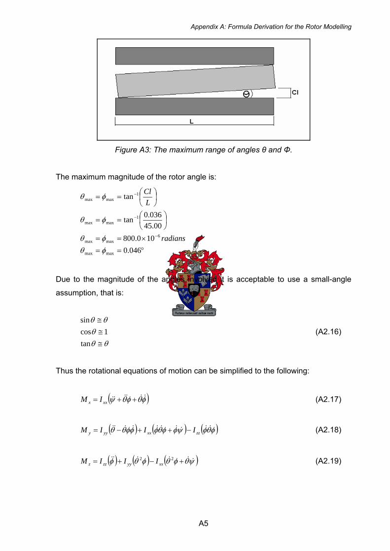
Appendix A: Formula Derivation for the Rotor Modelling
Figure A3: The maximum range of angles θ and Φ.
The maximum magnitude of the rotor angle is:
°==×==
⎟⎠⎞
⎜⎝⎛==
⎟⎠⎞
⎜⎝⎛==
−
−
−
046.0100.800
00.45036.0tan
tan
maxmax
6maxmax
1maxmax
1maxmax
φθφθ
φθ
φθ
radians
LCl
Due to the magnitude of the angles involved it is acceptable to use a small-angle
assumption, that is:
θθθ
θθ
≅≅≅
tan1cos
sin (A2.16)
Thus the rotational equations of motion can be simplified to the following:
( )φθφθψ &&&&&& ++= xxx IM (A2.17)
( ) ( ) ( )φθφψφφθφφφθθ &&&&&&&&&&zzxxyyy IIIM −++−= (A2.18)
( ) ( ) ( )ψθφθφθφ &&&&&& +−+= 22xxyyzzz IIIM (A2.19)
A5
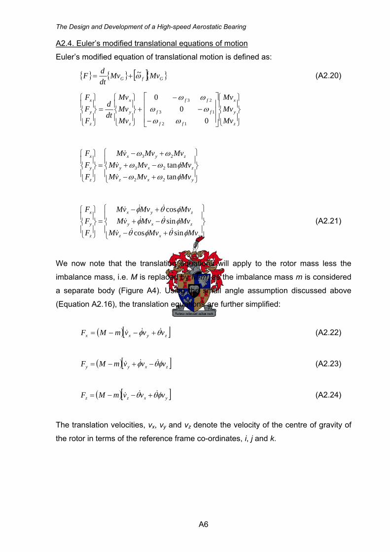
The Design and Development of a High-speed Aerostatic Bearing
A2.4. Euler’s modified translational equations of motion
Euler’s modified equation of translational motion is defined as:
{ } { } [ ]{ GfG MvMvdtdF ω~+= } (A2.20)
⎪⎭
⎪⎬
⎫
⎪⎩
⎪⎨
⎧
⎥⎥⎥
⎦
⎤
⎢⎢⎢
⎣
⎡
−−
−+
⎪⎭
⎪⎬
⎫
⎪⎩
⎪⎨
⎧=
⎪⎭
⎪⎬
⎫
⎪⎩
⎪⎨
⎧
z
y
x
ff
ff
ff
z
y
x
z
y
x
MvMvMv
MvMvMv
dtd
FFF
00
0
12
13
23
ωωωωωω
⎪⎭
⎪⎬
⎫
⎪⎩
⎪⎨
⎧
+−−++−
=⎪⎭
⎪⎬
⎫
⎪⎩
⎪⎨
⎧
yxz
zxy
zyx
z
y
x
MvMvvMMvMvvM
MvMvvM
FFF
φωωφωω
ωω
tantan
22
23
23
&
&
&
⎪⎭
⎪⎬
⎫
⎪⎩
⎪⎨
⎧
+−−++−
=⎪⎭
⎪⎬
⎫
⎪⎩
⎪⎨
⎧
yxz
zxy
zyx
z
y
x
MvMvvMMvMvvMMvMvvM
FFF
φθφθφθφφθφ
sincossincos
&&&
&&&
&&&
(A2.21)
We now note that the translation equations will apply to the rotor mass less the
imbalance mass, i.e. M is replaced by M-m, as the imbalance mass m is considered
a separate body (Figure A4). Using the small angle assumption discussed above
(Equation A2.16), the translation equations are further simplified:
( )[ ]zyxx vvvmMF θφ &&& +−−= (A2.22)
( )[ ]zxyy vvvmMF φθφ &&& −+−= (A2.23)
( )[ ]yxzz vvvmMF φθθ &&& +−−= (A2.24)
The translation velocities, vx, vy and vz denote the velocity of the centre of gravity of
the rotor in terms of the reference frame co-ordinates, i, j and k.
A6
Appendix A: Formula Derivation for the Rotor Modelling
A3. The forces applied to the rotor
The forces which are applied to the rotor are shown in Figure A4 below.
Figure A4: Forces applied to the rotor.
The forces applied to the rotor are as follows:
• Forces from the two turbine nozzles, Ffw1 and Ffw2 for clockwise rotor rotation
(positive i) or Fbw1 and Fbw2 for counter clockwise rotation (negative i).
• Forces due to an imbalance present in the rotor, Fx, Fy and Fz.
• A normal cutting force on the blade, Fcut.
• A corresponding friction force, Ffric.
• The weight of the rotor, W.
A3.1. The turbine-drive forces
The force of the airflow on the turbine pockets from a single nozzle is defined as:
( tnBEFturb )ψ&sin+= (N) (A3.1)
It consists of a mean force E over which a small oscillation occurs with magnitude B.
The oscillation is due to the presence of a finite number of turbine pockets, and its
frequency is equal to the product of the number of pockets n (which is 30 in this
particular case) and the rotor speed ψ& . Because there are two nozzles present for
each drive direction the nozzle forces should, in theory, be completely in balance.
The resultant turbine force responsible for rotor translation should thus be zero.
A7
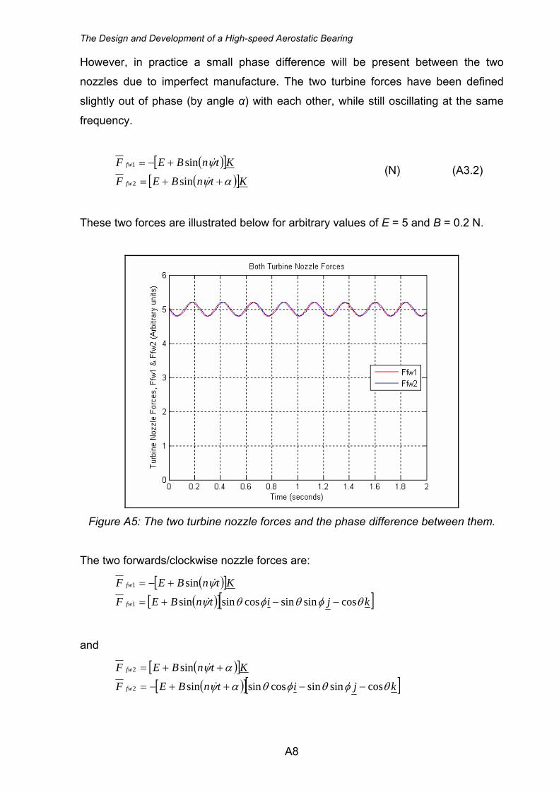
The Design and Development of a High-speed Aerostatic Bearing
However, in practice a small phase difference will be present between the two
nozzles due to imperfect manufacture. The two turbine forces have been defined
slightly out of phase (by angle α) with each other, while still oscillating at the same
frequency.
( )[ ]( )[ ]KtnBEF
KtnBEF
fw
fw
αψ
ψ
++=
+−=
&
&
sin
sin
2
1 (N) (A3.2)
These two forces are illustrated below for arbitrary values of E = 5 and B = 0.2 N.
Figure A5: The two turbine nozzle forces and the phase difference between them.
The two forwards/clockwise nozzle forces are:
( )[ ]( )[ ][ ]kjitnBEF
KtnBEF
fw
fw
θφθφθψ
ψ
cossinsincossinsin
sin
1
1
−−+=
+−=
&
&
and
( )[ ]( )[ ][ ]kjitnBEF
KtnBEF
fw
fw
θφθφθαψ
αψ
cossinsincossinsin
sin
2
2
−−++−=
++=
&
&
A8
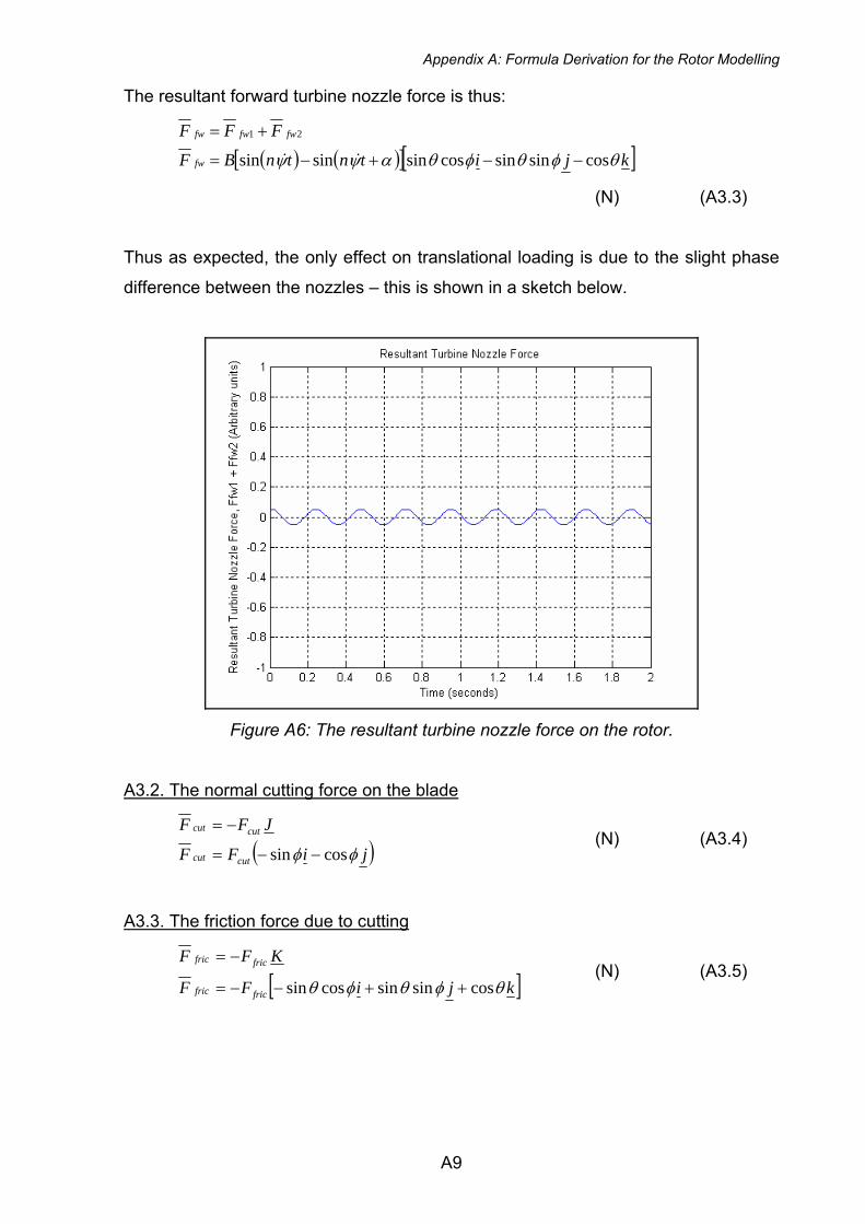
Appendix A: Formula Derivation for the Rotor Modelling
The resultant forward turbine nozzle force is thus:
( ) ( )[ ][ ]kjitntnBF
FFF
fw
fwfwfw
θφθφθαψψ cossinsincossinsinsin21
−−+−=
+=
&&
(N) (A3.3)
Thus as expected, the only effect on translational loading is due to the slight phase
difference between the nozzles – this is shown in a sketch below.
Figure A6: The resultant turbine nozzle force on the rotor.
A3.2. The normal cutting force on the blade
( jiFF
JFF
cutcut
cutcut
φφ cossin −−=
−=
) (N) (A3.4)
A3.3. The friction force due to cutting
[ kjiFF
KFF
fricfric
fricfric
θφθφθ cossinsincossin ++−−=
−=
] (N) (A3.5)
A9
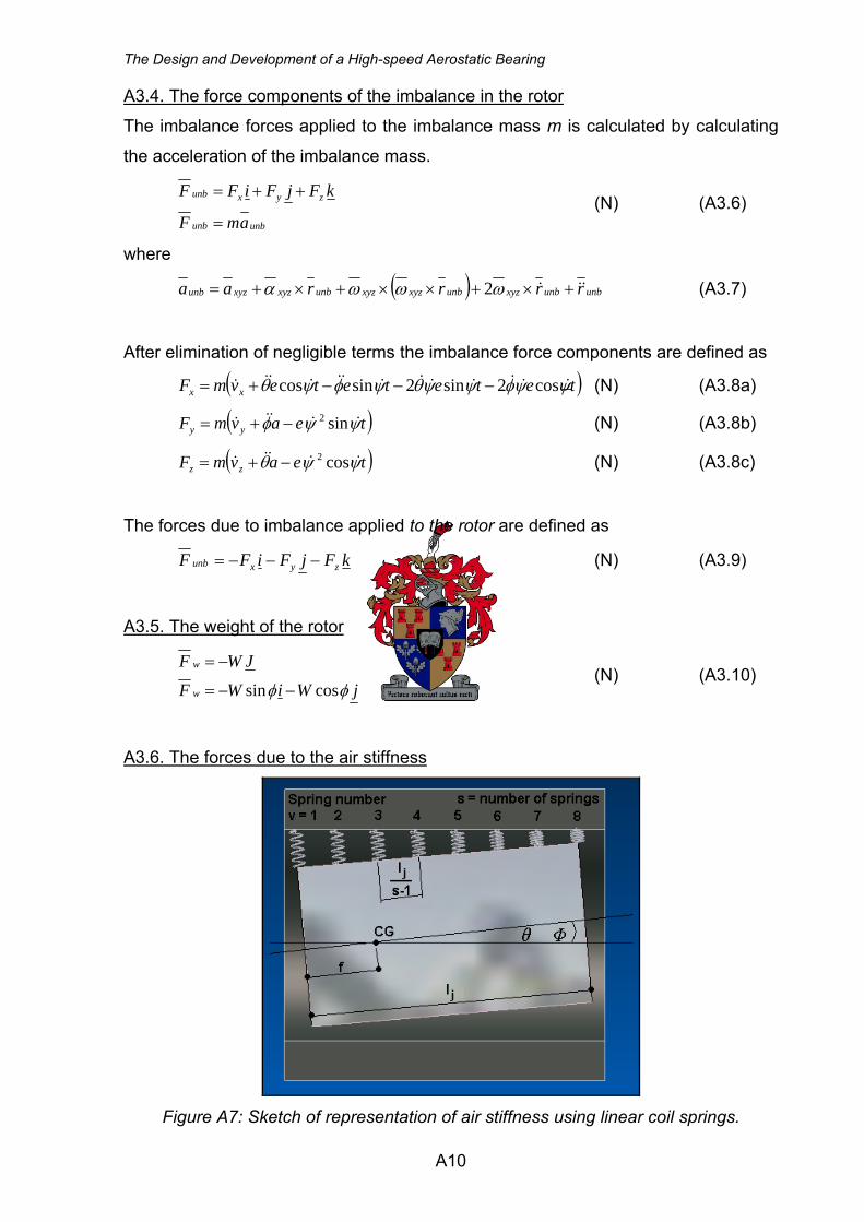
The Design and Development of a High-speed Aerostatic Bearing
A3.4. The force components of the imbalance in the rotor
The imbalance forces applied to the imbalance mass m is calculated by calculating
the acceleration of the imbalance mass.
unbunb
zyxunb
amF
kFjFiFF
=
++= (N) (A3.6)
where
( ) unbunbxyzunbxyzxyzunbxyzxyzunb rrrraa &&& +×+××+×+= ωωωα 2 (A3.7)
After elimination of negligible terms the imbalance force components are defined as
( )tetetetevmF xx ψψφψψθψφψθ &&&&&&&&&&&&& cos2sin2sincos −−−+= (N) (A3.8a)
( )teavmF yy ψψφ &&&&& sin2−+= (N) (A3.8b)
( )teavmF zz ψψθ &&&&& cos2−+= (N) (A3.8c)
The forces due to imbalance applied to the rotor are defined as
kFjFiFF zyxunb −−−= (N) (A3.9)
A3.5. The weight of the rotor
jWiWF
JWF
w
w
φφ cossin −−=
−= (N) (A3.10)
A3.6. The forces due to the air stiffness
Figure A7: Sketch of representation of air stiffness using linear coil springs.
A10
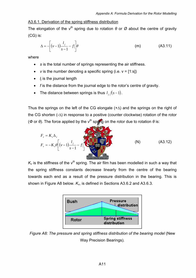
Appendix A: Formula Derivation for the Rotor Modelling
A3.6.1. Derivation of the spring stiffness distribution
The elongation of the vth spring due to rotation θ or Ø about the centre of gravity
(CG) is:
( ) θ⎥⎦
⎤⎢⎣
⎡−
−−−=Δ f
sl
v j
11 (m) (A3.11)
where
• s is the total number of springs representing the air stiffness.
• v is the number denoting a specific spring (i.e. v = [1:s])
• lj is the journal length
• f is the distance from the journal edge to the rotor’s centre of gravity.
• The distance between springs is thus ( )1−sl j .
Thus the springs on the left of the CG elongate (+∆) and the springs on the right of
the CG shorten (-∆) in response to a positive (counter clockwise) rotation of the rotor
(Φ or θ). The force applied by the vth spring on the rotor due to rotation θ is:
( ) ⎥⎦
⎤⎢⎣
⎡−
−−−=
Δ=
fsl
vKF
KF
jvv
vvv
11θ
(N) (A3.12)
Kv is the stiffness of the vth spring. The air film has been modelled in such a way that
the spring stiffness constants decrease linearly from the centre of the bearing
towards each end as a result of the pressure distribution in the bearing. This is
shown in Figure A8 below. Kv, is defined in Sections A3.6.2 and A3.6.3.
Figure A8: The pressure and spring stiffness distribution of the bearing model (New
Way Precision Bearings).
A11
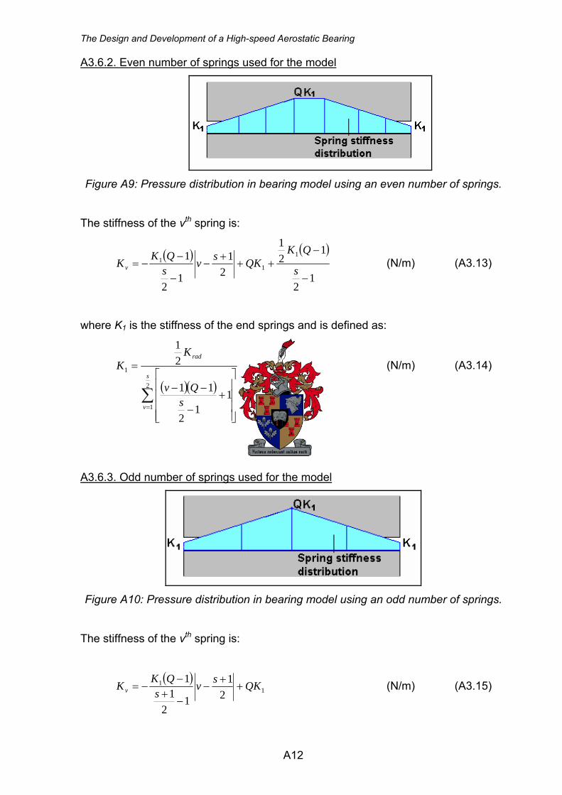
The Design and Development of a High-speed Aerostatic Bearing
A3.6.2. Even number of springs used for the model
Figure A9: Pressure distribution in bearing model using an even number of springs.
The stiffness of the vth spring is:
( ) ( )
12
121
21
12
1 1
11
−
−++
+−
−
−−=
s
QKQKsv
sQKKv (N/m) (A3.13)
where K1 is the stiffness of the end springs and is defined as:
( )( )∑=
⎥⎥⎥⎥
⎦
⎤
⎢⎢⎢⎢
⎣
⎡
+−
−−
=
2
1
1
11
2
11
21
s
v
rad
sQv
KK (N/m) (A3.14)
A3.6.3. Odd number of springs used for the model
Figure A10: Pressure distribution in bearing model using an odd number of springs.
The stiffness of the vth spring is:
( )1
1
21
12
11 QKsv
sQKKv +
+−
−+
−−= (N/m) (A3.15)
A12
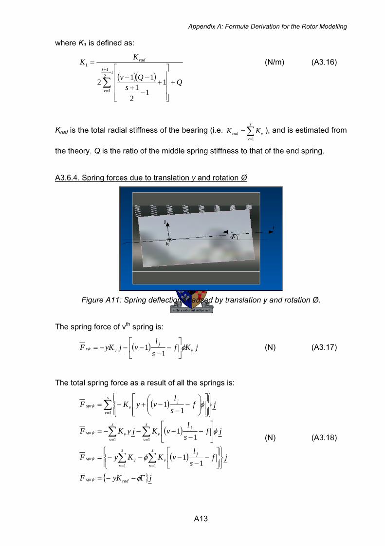
Appendix A: Formula Derivation for the Rotor Modelling
where K1 is defined as:
( )( ) Qs
Qv
KK
s
v
rad
+
⎥⎥⎥⎥
⎦
⎤
⎢⎢⎢⎢
⎣
⎡
+−
+−−
=
∑−
+
=
121
1
1
11
21
112
(N/m) (A3.16)
Krad is the total radial stiffness of the bearing (i.e. ), and is estimated from
the theory. Q is the ratio of the middle spring stiffness to that of the end spring.
∑=
=s
vvrad KK
1
A3.6.4. Spring forces due to translation y and rotation Ø
Figure A11: Spring deflections caused by translation y and rotation Ø.
The spring force of vth spring is:
( ) jKfsl
vjyKF vj
vv φφ ⎥⎦
⎤⎢⎣
⎡−
−−−−=
11 (N) (A3.17)
The total spring force as a result of all the springs is:
( )
( )
( )
{ }jyKF
jfsl
vKKyF
jfsl
vKjyKF
jfsl
vyKF
radspr
s
v
jv
s
vvspr
s
v
s
v
jvvspr
s
v
jvspr
Γ−−=
⎪⎭
⎪⎬⎫
⎪⎩
⎪⎨⎧
⎥⎦
⎤⎢⎣
⎡−
−−−−=
⎥⎦
⎤⎢⎣
⎡−
−−−−=
⎪⎭
⎪⎬⎫
⎪⎩
⎪⎨⎧
⎥⎥⎦
⎤
⎢⎢⎣
⎡⎟⎟⎠
⎞⎜⎜⎝
⎛−
−−+−=
∑∑
∑ ∑
∑
==
= =
=
φ
φ
φ
φ
φ
φ
φ
φ
11
1 1
1
11
11
11
(N) (A3.18)
A13
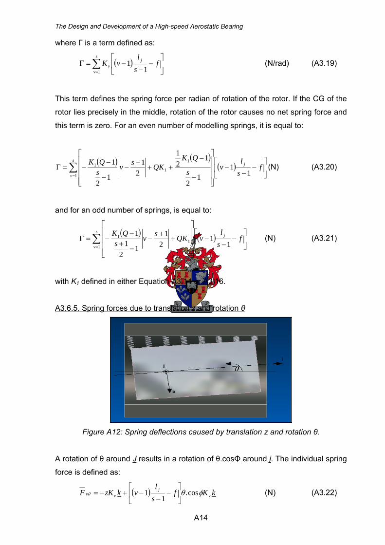
The Design and Development of a High-speed Aerostatic Bearing
where Γ is a term defined as:
( )∑=
⎥⎦
⎤⎢⎣
⎡−
−−=Γ
s
v
jv f
sl
vK1 1
1 (N/rad) (A3.19)
This term defines the spring force per radian of rotation of the rotor. If the CG of the
rotor lies precisely in the middle, rotation of the rotor causes no net spring force and
this term is zero. For an even number of modelling springs, it is equal to:
( ) ( )( )∑
=⎥⎦
⎤⎢⎣
⎡−
−−
⎥⎥⎥⎥
⎦
⎤
⎢⎢⎢⎢
⎣
⎡
−
−++
+−
−
−−=Γ
s
v
j fsl
vs
QKQKsv
sQK
1
1
11
11
12
121
21
12
1 (N) (A3.20)
and for an odd number of springs, is equal to:
( ) ( )∑=
⎥⎦
⎤⎢⎣
⎡−
−−
⎥⎥⎥⎥
⎦
⎤
⎢⎢⎢⎢
⎣
⎡
++
−−
+−
−=Γs
v
j fsl
vQKsvs
QK1
11
11
21
12
11 (N) (A3.21)
with K1 defined in either Equation A3.14 or A3.16.
A3.6.5. Spring forces due to translation z and rotation θ
Figure A12: Spring deflections caused by translation z and rotation θ.
A rotation of θ around J results in a rotation of θ.cosΦ around j. The individual spring
force is defined as:
( ) kKfsl
vkzKF vj
vv φθθ cos.1
1 ⎥⎦
⎤⎢⎣
⎡−
−−+−= (N) (A3.22)
A14
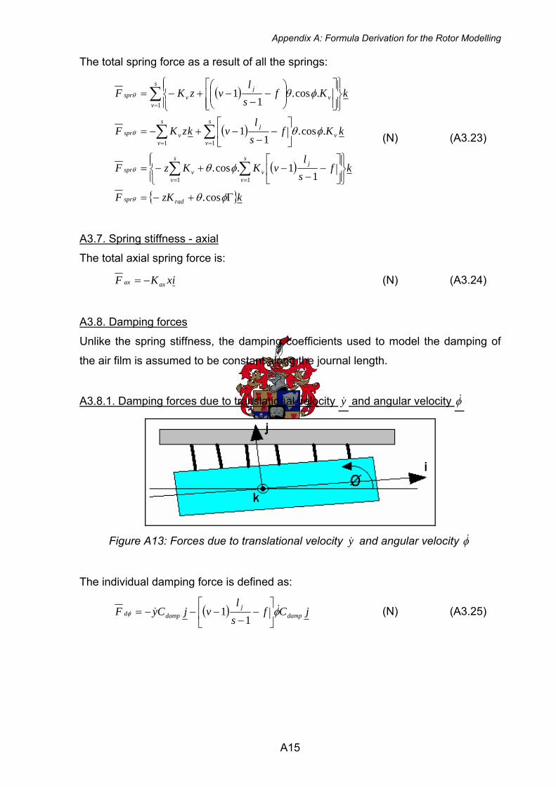
Appendix A: Formula Derivation for the Rotor Modelling
The total spring force as a result of all the springs:
( )
( )
( )
{ }kzKF
kfsl
vKKzF
kKfsl
vkzKF
kKfsl
vzKF
radspr
s
v
jv
s
vvspr
s
v
s
vv
jvspr
s
vv
jvspr
Γ+−=
⎪⎭
⎪⎬⎫
⎪⎩
⎪⎨⎧
⎥⎦
⎤⎢⎣
⎡−
−−+−=
⎥⎦
⎤⎢⎣
⎡−
−−+−=
⎪⎭
⎪⎬⎫
⎪⎩
⎪⎨⎧
⎥⎥⎦
⎤
⎢⎢⎣
⎡⎟⎟⎠
⎞⎜⎜⎝
⎛−
−−+−=
∑∑
∑ ∑
∑
==
= =
=
φθ
φθ
φθ
φθ
θ
θ
θ
θ
cos.
11.cos.
.cos.1
1
.cos.1
1
11
1 1
1
(N) (A3.23)
A3.7. Spring stiffness - axial
The total axial spring force is:
ixKF axax −= (N) (A3.24)
A3.8. Damping forces
Unlike the spring stiffness, the damping coefficients used to model the damping of
the air film is assumed to be constant along the journal length.
A3.8.1. Damping forces due to translational velocity y& and angular velocity φ&
Figure A13: Forces due to translational velocity and angular velocity y& φ&
The individual damping force is defined as:
( ) jCfsl
vjCyF dampj
dampd φφ && ⎥⎦
⎤⎢⎣
⎡−
−−−−=
11 (N) (A3.25)
A15
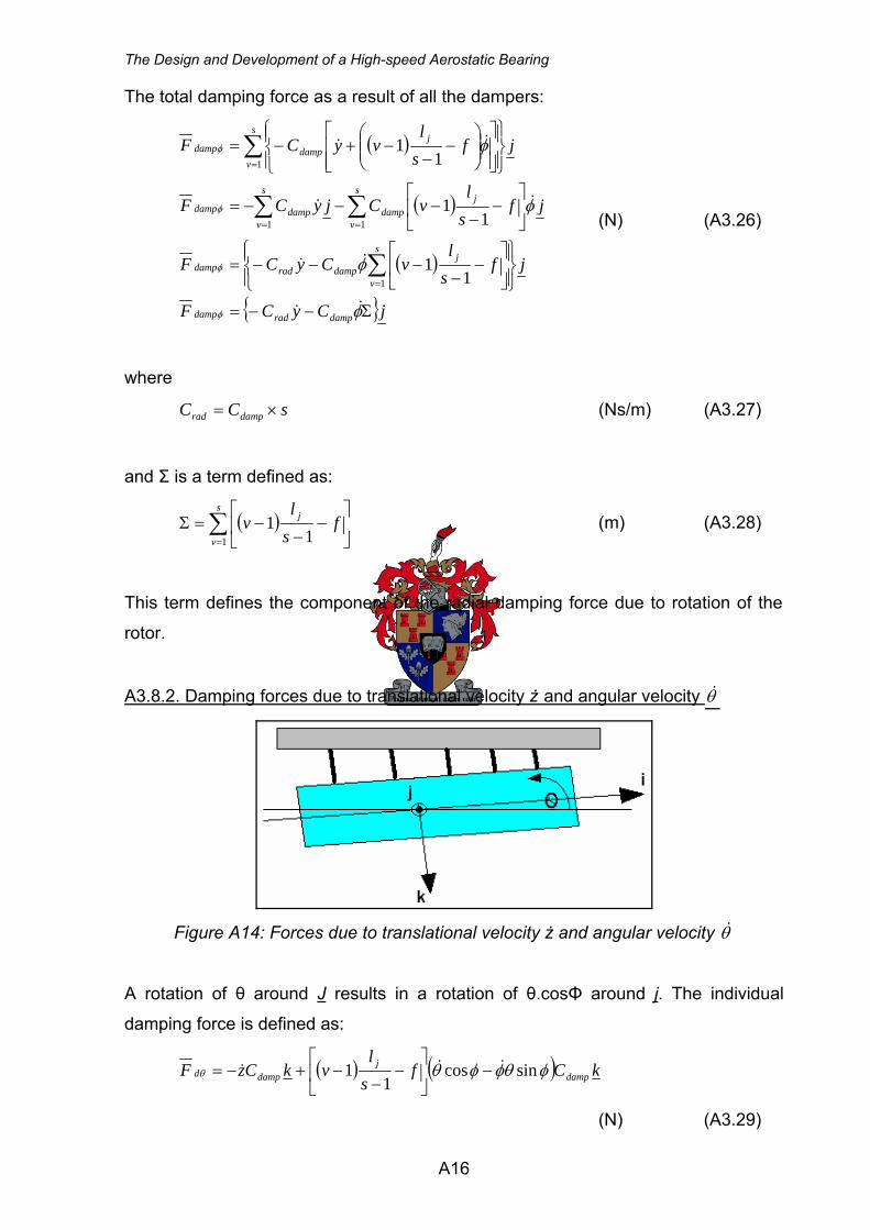
The Design and Development of a High-speed Aerostatic Bearing
The total damping force as a result of all the dampers:
( )
( )
( )
{ }jCyCF
jfsl
vCyCF
jfsl
vCjyCF
jfsl
vyCF
dampraddamp
s
v
jdampraddamp
s
v
s
v
jdampdampdamp
s
v
jdampdamp
Σ−−=
⎪⎭
⎪⎬⎫
⎪⎩
⎪⎨⎧
⎥⎦
⎤⎢⎣
⎡−
−−−−=
⎥⎦
⎤⎢⎣
⎡−
−−−−=
⎪⎭
⎪⎬⎫
⎪⎩
⎪⎨⎧
⎥⎥⎦
⎤
⎢⎢⎣
⎡⎟⎟⎠
⎞⎜⎜⎝
⎛−
−−+−=
∑
∑ ∑
∑
=
= =
=
φ
φ
φ
φ
φ
φ
φ
φ
&&
&&
&&
&&
1
1 1
1
11
11
11
(N) (A3.26)
where
sCC damprad ×= (Ns/m) (A3.27)
and Σ is a term defined as:
( )∑=
⎥⎦
⎤⎢⎣
⎡−
−−=Σ
s
v
j fsl
v1 1
1 (m) (A3.28)
This term defines the component of the radial damping force due to rotation of the
rotor.
A3.8.2. Damping forces due to translational velocity ż and angular velocity θ&
Figure A14: Forces due to translational velocity ż and angular velocity θ&
A rotation of θ around J results in a rotation of θ.cosΦ around j. The individual
damping force is defined as:
( ) ( ) kCfsl
vkCzF dampj
dampd φθφφθθ sincos1
1 &&& −⎥⎦
⎤⎢⎣
⎡−
−−+−=
(N) (A3.29)
A16
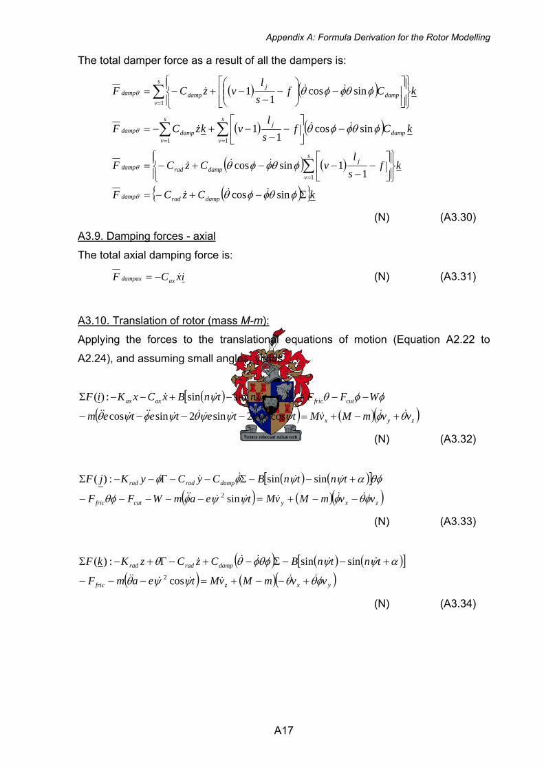
Appendix A: Formula Derivation for the Rotor Modelling
The total damper force as a result of all the dampers is:
( ) ( )
( ) ( )
( ) ( )
( ){ }kCzCF
kfsl
vCzCF
kCfsl
vkzCF
kCfsl
vzCF
dampraddamp
s
v
jdampraddamp
s
v
s
vdamp
jdampdamp
s
vdamp
jdampdamp
Σ−+−=
⎪⎭
⎪⎬⎫
⎪⎩
⎪⎨⎧
⎥⎦
⎤⎢⎣
⎡−
−−−+−=
−⎥⎦
⎤⎢⎣
⎡−
−−+−=
⎪⎭
⎪⎬⎫
⎪⎩
⎪⎨⎧
⎥⎥⎦
⎤
⎢⎢⎣
⎡−⎟⎟
⎠
⎞⎜⎜⎝
⎛−
−−+−=
∑
∑ ∑
∑
=
= =
=
φθφφθ
φθφφθ
φθφφθ
φθφφθ
θ
θ
θ
θ
sincos
11sincos
sincos1
1
sincos1
1
1
1 1
1
&&&
&&&
&&&
&&&
(N) (A3.30)
A3.9. Damping forces - axial
The total axial damping force is:
ixCF axdampax &−= (N) (A3.31)
A3.10. Translation of rotor (mass M-m):
Applying the forces to the translational equations of motion (Equation A2.22 to
A2.24), and assuming small angles, yields:
( ) ( )[ ]( ) ( )( zyx
cutfricaxax
vvmMvMtetetetem
WFFtntnBxCxKiF
θφψψφψψθψφψθ )φφθθαψψ
&&&&&&&&&&&&&&&
&&&
+−+=−−−−
−−++−+−−Σ
cos2sin2sincos
sinsin:)(
(N) (A3.32)
( ) ( )[ ]( ) ( )( zxycutfric
dampradrad
vvmMvMteamWFF
tntnBCyCyKjF
φθφψψφθφ
θφαψψφφ&&&&&&&
&&&&
−−+=−−−−−
+−−Σ−−Γ−−Σ
sin
sinsin:)(2 )
(N) (A3.33)
( ) ( ) ( )[ ]( ) ( )( )yxzfric
dampradrad
vvmMvMteamF
tntnBCzCzKkF
φθθψψθ
αψψθφφθθ&&&&&&&
&&&&&
+−−+=−−−
+−−Σ−+−Γ+−Σ
cos
sinsin:)(2
(N) (A3.34)
A17
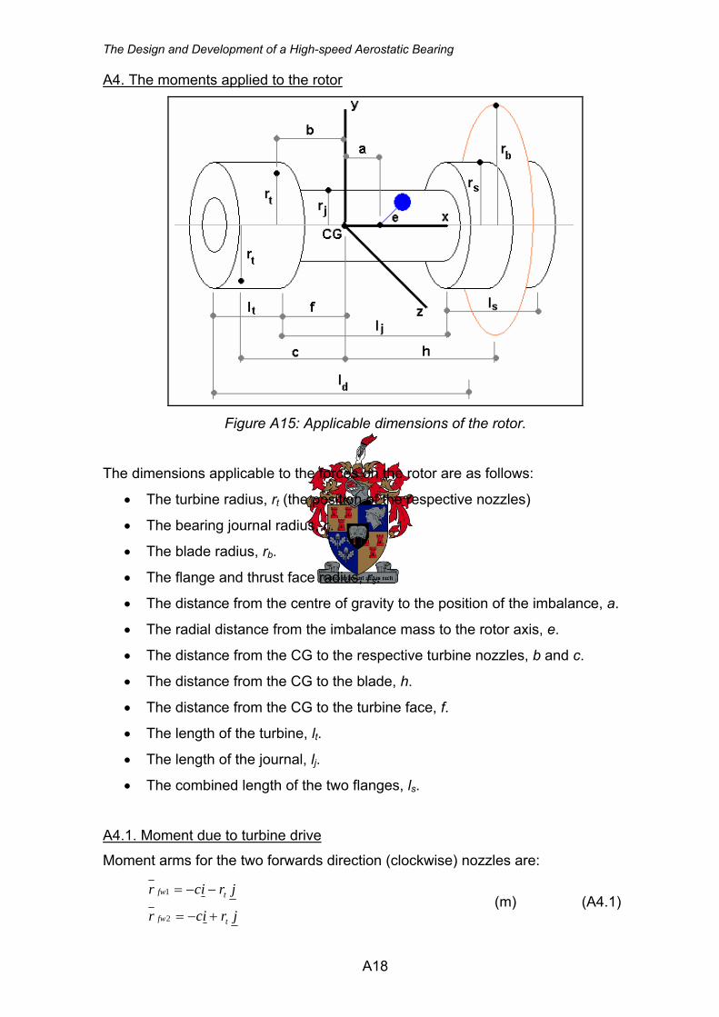
The Design and Development of a High-speed Aerostatic Bearing
A4. The moments applied to the rotor
Figure A15: Applicable dimensions of the rotor.
The dimensions applicable to the forces on the rotor are as follows:
• The turbine radius, rt (the position of the respective nozzles)
• The bearing journal radius, rj.
• The blade radius, rb.
• The flange and thrust face radius, rs.
• The distance from the centre of gravity to the position of the imbalance, a.
• The radial distance from the imbalance mass to the rotor axis, e.
• The distance from the CG to the respective turbine nozzles, b and c.
• The distance from the CG to the blade, h.
• The distance from the CG to the turbine face, f.
• The length of the turbine, lt.
• The length of the journal, lj.
• The combined length of the two flanges, ls.
A4.1. Moment due to turbine drive
Moment arms for the two forwards direction (clockwise) nozzles are:
jricr
jricr
tfw
tfw
+−=
−−=
2
1 (m) (A4.1)
A18
Appendix A: Formula Derivation for the Rotor Modelling
Resulting moment:
[ ] ( )[ ][ ][ ] ( )[ ][ ]kjitnBEjric
kjitnBEjricT
FrFrT
t
tfw
fwfwfwfwfw
θφθφθαω
θφθφθω
cossinsincossinsin
cossinsincossinsin2211
−−++−×+−+
−−+×−−=
×+×=
( )[ ] ( )[ ]( )[ ] ( )[ ]( )[ ] ( )[ ]( )[ ] ( )[ ] itnBErktnBEr
jtnBEcktnBEcitnBErktnBEr
jtnBEcktnBEcT
tt
tt
fw
θαωφθαω
θαωφθαωθωφθω
θωφθω
cossincossinsin
cossinsinsinsincossincossinsin
cossinsinsinsin
++++++
+++++−++++
+−+=
( ) ( )( )[ ]{ }( ) ( )( )[ ]{ }( ) ( )( )[ ] ( ) ( )( )[ ]{ }ktntnBErtntnBc
jtntnBcitntnBErT
t
tfw
φθαωωφθαωω
θωαωθαωω
cossinsinsin2sinsinsinsin
cossinsincossinsin2
+++++−+
−+++++=
(N·m) (A4.2)
A4.2. Moment due to cutting force
Moment arm:
jrihr bcut += (m) (A4.3)
Resulting moment:
[ ] [ ]
[ ]khFFrT
kFrkhFT
jiFjrihT
FrT
cutcutbcut
cutbcutcut
cutbcut
cutcutcut
φφ
φφ
φφ
cossin
sincos
cossin
−=
+−=
−−×+=
×=
(N·m) (A4.4)
A4.3. Moment due to frictional force
Moment arm:
jrihr bfric += (m) (A4.5)
A19
The Design and Development of a High-speed Aerostatic Bearing
Resulting moment for forwards (clockwise) direction:
[ ] [ ]
( )kFrhFjhFiFrT
iFrkFrjhFkhFT
kjiFjrihT
FrT
fricbfricfricfricbfric
fricbfricbfricfricfric
fricbfric
fricfricfric
φθφθθθ
θφθθφθ
θφθφθ
cossinsinsincoscos
coscossincossinsin
cossinsincossin
−−++−=
−−+−=
−−×+=
×=
(N·m) (A4.6)
A4.4. Moment due to rotor imbalance
Moment arm:
ktejteiarunb ψψ && cossin ++= (m) (A4.7)
Resulting moment:
( ) ( )( ) ( ) ( )kaFteFjteFaFiteFteFT
kFjFiFktejteiaT
FrT
yxxzzyunb
zyxunb
unbunbunb
−+−+−=
−−−×++=
×=
ψψψψ
ψψ
&&&&
&&
sincossincos
cossin
(N·m) (A4.8)
where the imbalance forces Fx, Fy and Fz are defined in Equations A3.8a to A3.8c.
Thus Equation A4.8 is rewritten more completely as:
( ) ( )( )( ) ( )( )( )( )( ) kteavamtetetetetevm
jtetetetetevmteavam
iteteavmteteavmT
yx
xz
zyunb
ψψφψψψφψψθψφψθ
ψψψφψψθψφψθψψθ
ψψψθψψψφ
&&&&&&&&&&&&&&&&&&&
&&&&&&&&&&&&&&&&&&&
&&&&&&&&&&&&
sinsincos2sin2sincos
coscos2sin2sincoscos
sincoscossin
2
2
22
−+−−−−++
−−−+−−++
−+−−+=
(N·m) (A4.9)
A4.5. Moments due to spring forces
A4.5.1 Moment due to translation y and rotation Ø
Moment arm:
( ) jrifsl
vr jj +⎥
⎦
⎤⎢⎣
⎡−
−−=
11φ (m) (A4.10)
A20
Appendix A: Formula Derivation for the Rotor Modelling
Resulting moment of all the springs:
[ ]
( ) ( )
( ) ( )
( ) ( )
[ ]kKyT
kfsl
vKkfsl
vyKT
kfsl
vyKfsl
vT
jfsl
vKyKjrifsl
vT
FrT
angspr
s
v
s
v
jv
jvspr
s
v
jv
jspr
s
v
jvvj
jspr
s
vvspr
φ
φ
φ
φ
φ
φ
φ
φ
φφφ
−Γ−=
⎥⎦
⎤⎢⎣
⎡−
−−−⎥
⎦
⎤⎢⎣
⎡−
−−−=
⎥⎥⎦
⎤
⎢⎢⎣
⎡⎟⎟⎠
⎞⎜⎜⎝
⎛⎟⎟⎠
⎞⎜⎜⎝
⎛−
−−+−⎥
⎦
⎤⎢⎣
⎡−
−−=
⎪⎭
⎪⎬⎫
⎪⎩
⎪⎨⎧
⎥⎦
⎤⎢⎣
⎡−
−−−−×
⎪⎭
⎪⎬⎫
⎪⎩
⎪⎨⎧
+⎥⎦
⎤⎢⎣
⎡−
−−=
×=
∑ ∑
∑
∑
∑
= =
=
=
=
1 1
2
1
1
1
11
11
11
11
11
11
(N·m) (A4.11)
The function Γ has been defined in Equation A3.19 – in this instance it defines the
component of the moment due to rotor translation. If the rotor’s centre of gravity falls
in the middle of the journal, translation has no effect on spring torque and this term is
zero. The angular stiffness, Kang, is defined as:
( )2
1 11∑
=⎥⎦
⎤⎢⎣
⎡−
−−=
s
v
jvang f
sl
vKK (N·m/rad) (A4.12)
Thus the angular stiffness is proportional to the radial stiffness and to the square of
the journal length, as described in the literature (Powell, 1970). It is also seen to be
dependent on the position of the CG.
A4.5.2. Moment due to translation z and rotation θ
Moment arm:
( ) krifsl
vr jj −⎥
⎦
⎤⎢⎣
⎡−
−−=
11θ (m) (A4.13)
A21
The Design and Development of a High-speed Aerostatic Bearing
Resulting moment of all the springs:
[ ]
( ) ( )
( ) ( )
( ) ( )
[ ]jKzT
jKfsl
vjfsl
vzKT
jKfsl
vfsl
vzKT
kfsl
vKzKkrifsl
vT
FrT
angspr
s
v
s
vv
jjvspr
s
vv
jjvspr
s
v
jvvj
jspr
s
vvspr
φθ
φθ
φθ
φθ
θ
θ
θ
θ
θθθ
cos
cos1
11
1
cos1
11
1
11cos
11
1 1
2
1
2
1
1
−Γ=
⎥⎦
⎤⎢⎣
⎡−
−−−⎥
⎦
⎤⎢⎣
⎡−
−−=
⎪⎭
⎪⎬⎫
⎪⎩
⎪⎨⎧
⎥⎦
⎤⎢⎣
⎡−
−−+⎥
⎦
⎤⎢⎣
⎡−
−−−−=
⎪⎭
⎪⎬⎫
⎪⎩
⎪⎨⎧
⎥⎦
⎤⎢⎣
⎡−
−−+−×
⎪⎭
⎪⎬⎫
⎪⎩
⎪⎨⎧
−⎥⎦
⎤⎢⎣
⎡−
−−=
×=
∑ ∑
∑
∑
∑
= =
=
=
=
(N·m) (A4.14)
A4.6. Moments due to damping forces
A4.6.1. Moment due to translational velocity y& and angular velocity φ&
Moment arm:
( ) jrifsl
vr jj +⎥
⎦
⎤⎢⎣
⎡−
−−=
11φ (m) (A4.15)
Resulting moment:
[ ]
( ) ( )
( ) ( )
( ) ( )
[ ]kCCyT
kfsl
vCkCyfsl
vT
kfsl
vCCyfsl
vT
jfsl
vCCyjrifsl
vT
FrT
dampdampdamp
s
v
s
v
jdampsprdamp
jdamp
s
v
jdampdamp
jdamp
s
v
jdampdampj
jdamp
s
vddamp
ΣΣ−Σ−=
⎥⎦
⎤⎢⎣
⎡−
−−−⎥
⎦
⎤⎢⎣
⎡−
−−−=
⎥⎥⎦
⎤
⎢⎢⎣
⎡⎟⎟⎠
⎞⎜⎜⎝
⎛−
−−−−⎥
⎦
⎤⎢⎣
⎡−
−−=
⎪⎭
⎪⎬⎫
⎪⎩
⎪⎨⎧
⎥⎦
⎤⎢⎣
⎡−
−−−−×
⎪⎭
⎪⎬⎫
⎪⎩
⎪⎨⎧
+⎥⎦
⎤⎢⎣
⎡−
−−=
×=
∑ ∑
∑
∑
∑
= =
=
=
=
φ
φ
φ
φ
φ
φ
φ
φ
φφφ
&&
&&
&&
&&
1 1
2
1
1
1
11
11
11
11
11
11
(N·m) (A4.16)
The function ΣΣ, is defined as:
( )2
1 11∑
=⎥⎦
⎤⎢⎣
⎡−
−−=ΣΣ
s
v
j fsl
v (m2) (A4.17)
This term relates the total radial coefficient to the angular damping coefficient.
A22
Appendix A: Formula Derivation for the Rotor Modelling
A4.6.2. Moment due to translational velocity ż and angular velocity θ&
Moment arm:
( ) krifsl
vr jj −⎥
⎦
⎤⎢⎣
⎡−
−−=
11θ (m) (A4.18)
Resulting moment of all the springs:
[ ]
( ) ( ) ( )
( ) ( ) ( )
( ) ( ) ( )
( )[ ]jCzCT
jCfsl
vjfsl
vzCT
jCfsl
vzCfsl
vT
kfsl
vCzCkrifsl
vT
FrT
dampdampdamp
s
v
s
vdamp
jjdampdamp
s
vdamp
jdamp
jdamp
s
v
jdampdampj
jdamp
s
vddamp
ΣΣ−−Σ=
−⎥⎦
⎤⎢⎣
⎡−
−−−⎥
⎦
⎤⎢⎣
⎡−
−−=
⎪⎭
⎪⎬⎫
⎪⎩
⎪⎨⎧
⎥⎥⎦
⎤
⎢⎢⎣
⎡−⎟⎟
⎠
⎞⎜⎜⎝
⎛−
−−+−⎥
⎦
⎤⎢⎣
⎡−
−−−=
⎪⎭
⎪⎬⎫
⎪⎩
⎪⎨⎧
⎥⎦
⎤⎢⎣
⎡−
−−−+−×
⎪⎭
⎪⎬⎫
⎪⎩
⎪⎨⎧
−⎥⎦
⎤⎢⎣
⎡−
−−=
×=
∑ ∑
∑
∑
∑
= =
=
=
=
φθφφθ
φθφφθ
φθφφθ
φθφφθ
θ
θ
θ
θ
θθθ
sincos
sincos1
11
1
sincos1
11
1
11sincos
11
1 1
2
1
1
1
&&&
&&&
&&&
&&&
(N·m) (A4.19)
A4.7. Rotation of the rotor
Substituting the above moment definitions into the rotational equations of motion
(Equations A2.17 to A2.19) yields a complete set of equations. For the case of
moments around the x axis:
( ) ( ) ( )( )[ ] ( )( ) ( )φθφθψψψψθ
ψψψφθθαωω&&&&&&&&&&&&
&&&&&&
++=−+−
−++−+++Σ
xxz
yfricbt
Iteteavm
teteavmFrtntnBEriM
sincos
cossincoscossinsin2:2
2
(N·m) (A4.20)
As this analysis pertains to a rotor at constant speed (ψ&& mean = 0), the frictional
moment should equal the moment due to the mean turbine nozzle forces:
b
tfric
tbfric
rr
EF
ErrF
2
cos2cos
=
= θθ (N·m) (A4.21)
A23
The Design and Development of a High-speed Aerostatic Bearing
As so, assuming small angles, Equation A4.23 can be rewritten as:
( ) ( ) ( )( )[ ] ( )( ) ( )φθφθψψψψθ
ψψψφαωω&&&&&&&&&&&&
&&&&&&
++=−+−
−++++Σ
xxz
yt
Iteteavm
teteavmtntnBriM
sincos
cossinsinsin:2
2
(N·m) (A4.22)
which in itself means that any variation in rotor speed ψ& will be due to the oscillation
of the turbine nozzle forces. In addition, it is noted that:
cutfric FF μ= (N) (A4.23)
with μ representing the dynamic coefficient of friction between the blade and the
diamond - thus moment summations around the j and z axes are as follows:
( ) ( ) ( ) ( )[ ]( ) ( )
( ) ( ) ( ) ( )φθφψφφθφφφθθψ
ψψψφψψθψφψψμ
ωαωθφφθθ
&&&&&&&&&&&
&&&&&&&&&&&&&&
&&&
zzxxyyyy
xzcut
dampdampang
IIItmemaI
tetetetevmtevamFh
tntncBCCzKzjM
−++−+−=
−−−−−++
−++ΣΣ−−Σ+−ΓΣ
222
2
cos
coscos2sin2sincos
sinsin:
(N·m) (A4.24)
( ) ( ) ( )[ ]( ) ( )( )[ ]( )
( ) ( ) ( ) ( ψθφθφθψφψψ
ψψψφψψθψθθμ
θφμφθαψψ
θφαψψφφ
&&&&&&&&&&
&&&&&&&&&&&
&&
&&&&
+−+++=−−
−−++−
−−+++++
+−+ΣΣ−Σ−−Γ−Σ
222222 sinsin
sincos..2sin..2cos.
sinsin2
sinsin:
xxyyzzy
xcutb
cutcutcutbt
dampdampang
IImatmeItevam
tetetetevmFr
FhhFFrtntnBEr
tntncBCCyKykM
)
(N·m) (A4.25)
Equations A3.32 to A3.34 as well as A4.22, A4.24 and A4.25 form the basis for the
MATLAB Simulink model used to predict the rotor’s dynamic characteristics. As the
forces depend on the rotational motion and the moments are dependent on the
motion of the centre of gravity, a separate solution of the above equations of motion
is not possible.
A24
Appendix B: Aerostatic Bearing Design Calculations
This appendix contains the design procedure for the aerostatic bearing. All of the
equations stated below were sourced from the book by J. W. Powell, Design of
Aerostatic Bearings, either from the text or from plotted graphs (in which case the
equations were obtained by fitting curves to the available graphs).
B1. The input parameters
The following parameters are specified at the start of the design:
1. Journal diameter, D
2. Journal length, lj
3. The larger radius of the thrust face, rs
4. The mean radial clearance in the journal bearing, MRC
5. The mean axial clearance in the thrust bearing, MAC
6. The supply pressure, Po
7. An estimated value for the journal exhaust pressure, Pd2
8. Atmospheric pressure at thrust exhaust, Pa
9. The jet type, i.e. either annular or simple
10. The jet position, i.e. either quarter-station (j=0.25lj) or half-station (j=0.5lj)
11. The number of jets per row, u
12. The intended gauge pressure ratio of journal section, Kgo
13. The mean gas temperature, T
14. The gas specific heat ratio, γ 15. The gas constant, R
B2. The approximate load capacities from bearing dimensions
For D = 25.4 mm, 06.72688.9477.925.2679
*23
−+−= jjj l
llW (N) (B1)
For D = 50.8 mm, 12.136271.15504.14
*2
−+−= jj l
lW (N) (B2)
For D = 76.2 mm, 52.213038.18008.29
*2
−+−= jj l
lW (N) (B3)
For D = 101.6 mm, 15.180546.9338.19
*2
++= jj l
lW (N) (B4)
B1
The Design and Development of a High-speed Aerostatic Bearing
For D = 127 mm, 03.556882.7504.14
*2
++= jj l
lW (N) (B5)
The length is given in millimetres and the load capacity in Newtons. For bearing of
which the diameter falls between the above set points, linear interpolation is used to
obtain the approximate load capacity. The above load capacities apply to a bearing
using simple jets at quarter stations and it must be noted that the use of annular jets
can reduce the load capacity by as much as 30% (Powell, 1970). Half-station
bearings can reduce the load capacity by as much as 50% on bearings with large lj/D
ratios (see Section B6). The above load capacities correspond to a supply pressure
of 6.8 bar gauge and the following correction is required for other supply pressures:
8.6
* 2do PPWW
−×= (N) (B6)
where the supply and journal exhaust pressures are expressed in bars.
B3. The approximate bearing flow rate
The approximate gas flow rate for a journal bearing is:
jl
Dfr 628.9* = (l/min) (B7)
The following corrections factors apply to the flow rate:
For pressure, ( ) ( ) 26.0144.00433.0 22
21 +−−−= dodo PPPPk (B8)
where the supply and journal exhaust pressures are expressed in bars.
For the MRC (mm), 3
2 0127.0⎟⎠⎞
⎜⎝⎛=
MRCk (B9)
For the gauge pressure ratio, (B10) 0214.09793.0661.3 23 ++= gogo KKk
The corrected flow rate is then
321* kkkfrfr ×××= (l/min) (B11)
B2
Appendix B: Aerostatic Bearing Design Calculations
If half-station jets are used, the flow rate is effectively halved:
2frfrhalf = (l/min) (B12)
The above equations are used solely in the initial stages of the bearing design to
gain some insight into the approximate bearing size required for the application.
B4. The simple jet size from the MRC
Kgo=0.4, (mm) (B13) 0046.00506.5972.162* 2 −+= MRCMRCd
Kgo=0.6, (mm) (B14) 0043.06182.6872.283* 2 −+= MRCMRCd
Kgo=0.8, (mm) (B15) 0027.04218.916.425* 2 −+= MRCMRCd
where the MRC is in millimetres. For other gauge pressure ratios, linear interpolation
is used. The following correction factors apply to the jet diameter:
For the supply pressure, ( ) ( ) 5314.01847.00133.0 22
24 +−+−−= dodo PPPPk (B16)
For the number of jets, u
k 85 = , (B17)
where u is the number of jets
For the lj/D ratio, jl
Dk =6 (B18)
For the station position, j/lj, jl
k j
47 = (B19)
For the exhaust pressure ratio,
7696.211
485.1911
629.8011
77.16311
78.15611
932.56 2
2
2
3
2
4
2
5
28 +⎟⎟
⎠
⎞⎜⎜⎝
⎛++
−⎟⎟⎠
⎞⎜⎜⎝
⎛++
+⎟⎟⎠
⎞⎜⎜⎝
⎛++
−⎟⎟⎠
⎞⎜⎜⎝
⎛++
+⎟⎟⎠
⎞⎜⎜⎝
⎛++
−=o
d
o
d
o
d
o
d
o
d
PP
PP
PP
PP
PP
k
(B20)
where the supply and exhaust pressures are gauge pressures expressed in bars.
The correct jet diameter is thus:
87654* kkkkkdd ×××××= (mm) (B21)
B3
The Design and Development of a High-speed Aerostatic Bearing
B5. The annular jet size from the MRC
Kgo=0.4, (mm) (B22) 0114.08352.1728.14216.62705* 23 −+−= MRCMRCMRCd
Kgo=0.6, (mm) (B23) 0025.01096.048.1859* 2 −−= MRCMRCd
Kgo=0.8, (mm) (B24) 0066.013.38.4038* 2 +−= MRCMRCd
For other gauge pressure ratios, linear interpolation is used. The following correction
factors apply to the jet diameter:
For the supply pressure, ( ) ( ) 1546.0323.00197.0 22
24 +−+−−= dodo PPPPk (B25)
For the number of jets, u
k 85 = (B26)
For the lj/D ratio, jl
Dk =6 (B27)
For the station position, j/lj, jl
k j
47 = (B28)
For the exhaust pressure ratio,
5063.411
998.3311
17.12211
97.21811
8.18811
516.62 2
2
2
3
2
4
2
5
28 +⎟⎟
⎠
⎞⎜⎜⎝
⎛++
−⎟⎟⎠
⎞⎜⎜⎝
⎛++
+⎟⎟⎠
⎞⎜⎜⎝
⎛++
−⎟⎟⎠
⎞⎜⎜⎝
⎛++
+⎟⎟⎠
⎞⎜⎜⎝
⎛++
−=o
d
o
d
o
d
o
d
o
d
PP
PP
PP
PP
PP
k
(B29)
The correct jet diameter is thus:
87654* kkkkkdd ×××××= (mm) (B30)
B6. The theoretical load capacity – the load coefficient Cl
For 5.0=jl
j (half-station bearings)
5.11 <≤Dl j , 173.0
25.31
1+
−= D
lC
j
l (B31)
25.1 <<Dl j , 157.0
889.13
5.1+
−= D
lC
j
l (B32)
32 ≤<Dl j , 121.0
81.33
0.2+
−= D
lC
j
l (B33)
B4
Appendix B: Aerostatic Bearing Design Calculations
For 25.0=jl
j (quarter station bearings)
5.11 <≤Dl j , 266.0
333.83
1+
−= D
lC
j
l (B34)
25.1 <<Dl j , 260.0
316.26
5.1+
−= D
lC
j
l (B35)
32 ≤<Dl j , 241.0
493.14
0.2+
−= D
lC
j
l (B36)
The theoretical load capacity in Newtons is
)(1.0 2dojl PPDlCW −××××= (N) (B37)
where the length and diameter of the journal are expressed in millimetres and the
pressure drop over the journal is expressed in bars.
If annular jets are used:
WWannular ×= 7.0 (N) (B38)
The bearing radial stiffness is, MRC
WK rad2000
= (N/m) (B39)
where the load capacity is in Newtons, and the MRC is in millimetres.
Bearing angular stiffness, 6
2
1016××
= jradang
lKK (N·m/rad) (B40)
with the radial stiffness in Newtons per meter and the bearing length in millimetres.
B7. The theoretical flow rate
For Po-Pd2 = 0.68 bar, (kg/s) (B41) 986.0log171.3 1010* += MRCfr
For Po-Pd2 = 3.40 bar, (kg/s) (B42) 655.1log047.3 1010* += MRCfr
For Po-Pd2 = 6.12 bar, (kg/s) (B43) 994.1log033.3 1010* += MRCfr
B5
The Design and Development of a High-speed Aerostatic Bearing
The MRC is expressed in millimetres. For other pressure drops, linear interpolation
can be used. The following correction factors apply to the theoretical flow rate:
For the D/lj ratio, jl
Dk =9 (B44)
For the gauge pressure ratio, 0214.09793.0661.3 23 ++= gogo KKk
The applicable flow rate for a quarter station bearing is thus:
(kg/s) (B45) 39* kkfrfr ××=
and if a half-station jet position is used, the applicable flow rate is:
(kg/s) (B46) 39*5.0 kkfrfr ×××=
B8. The theoretical pressure drop over the jet
The jet area for simple jets is: 2
2000⎟⎠⎞
⎜⎝⎛=
dAsimple π (m2) (B47)
where d is the jet diameter in millimetres. The jet area for annular jets is:
6101×××
=MRCdAannular
π (m2) (B48)
where the MRC and jet diameter are in millimetres.
The velocity at the jet throat is defined as
ACuljfr
vdd
j
×××
××
=ρ
2 (m/s) (B49)
where the bearing flow rate fr is given in kg/s, Cd is the discharge coefficient (taken
as 0.8), ρd is the density at the throat of the jet (kg/m3) and A is the jet area (m2).
However the density at the throat is not know, as the pressure at the throat has not
yet been calculated – so at this stage an estimate of the density is used (Crowe,
2001).
B6
Appendix B: Aerostatic Bearing Design Calculations
The static pressure at the jet throat is defined as
( )1
15.273211)1(
12
2 −⎥⎥
⎦
⎤
⎢⎢
⎣
⎡
⎟⎟⎠
⎞⎜⎜⎝
⎛
+−
−+=−γγ
γγ
TRvPP od (bar, gauge) (B50)
with the supply pressure expressed in bars gauge and the gas temperature in
degrees Celsius.
The density at the throat using the calculated throat pressure, Pd2, is
γ
ρρ
1
11⎟⎟⎠
⎞⎜⎜⎝
⎛++
=o
dod P
P (kg/m3) (B51)
The new calculated density would be used to calculate a new iterated value for the
velocity, and so the iterations would continue until the change in calculated density is
within the desired precision. The critical pressure ratio over the jet is defined as
12
12
11 −
⎟⎟⎠
⎞⎜⎜⎝
⎛+
=++ γ
γ
γo
d
PP
which for air (γ = 1.4) is 0.528. The pressure ratio over the jet must be kept higher
than this value in order to ensure the jets are not choked, which could cause bearing
instability.
B9. The axial bearing load capacity and stiffness
Load capacity, ⎟⎠⎞
⎜⎝⎛
⎟⎟⎠
⎞⎜⎜⎝
⎛⎟⎟⎠
⎞⎜⎜⎝
⎛⎟⎠⎞
⎜⎝⎛ +⎟
⎠⎞
⎜⎝⎛−
×××=
Dr
DrDr
PWs
ss
dt 2ln2
12
ln22
1.0
22
2 π (N) (B52)
where D is the journal diameter (mm), rs is the larger thrust radius, and Pd2 is the
journal exhaust pressure in bars gauge.
Axial stiffness, MAC
WK t
ax2880
= , (N/m) (B53)
with the MAC expressed in millimetres.
B7
Appendix C: Computer Programs
C1. Bearing design program
%This program calculates specific parameters required for a successful aerostatic bearing design, using
%thrust faces fed by the journal exhaust. Jet position can be either 1/4 or 1/2 station. clear all close all clc %%Input Data%% D=25; %Journal diameter, mm L=45; %Journal length, mm b=25; %Maximum radius of thrust face, mm %Minimum radius is the shaft radius, D/2 ho=0.0180; %Mean radial clearance, mm ht=0.0300; %Mean axial clearance, mm Po=6.0; %Supply pressure, bar gauge Pd2=0.6; %Estimated journal exhaust pressure, bar gauge jet=['annular']; %Specify the jet type %jet=['simple.']; l=0.25*L; %Jet station, either 0.25 or 0.5 x L n=8; %Number of jets per row Kgo=0.7; %Desired gauge pressure ratio T=15; %Mean gas temperature, degrees Celcius k=1.4; %Specific heat ratio for gas R=287; %Gas constant, J/kg.K %%Reference data%% P_ref=6.8; %Reference supply pressure, bar gauge ho_ref=0.0254/2; %Reference journal clearance, mm %%Calculating the ball park load capacity%% u=2; if D>=127 disp(['Warning: Journal diameter is larger than calculations can predict.']) end if D<25.4 u=L^3/2679.25-L^2/9.477+9.688*L-72.061; ld=(D/25.4)*u;
C1
The Design and Development of a High-speed Aerostatic Bearing
elseif D>=25.4 & D<50.8 low=L^3/2679.25-L^2/9.477+9.688*L-72.061; u=-L^2/14.5038+15.271*L-136.1156; ld=((D-25.4)/25.4)*(u-low)+low; elseif D>=50.8 & D<76.2 low=-L^2/14.5038+15.271*L-136.1156; u=-L^2/29.008+18.0375*L-213.515; ld=((D-50.8)/25.4)*(u-low)+low; elseif D>=76.2 & D<101.6 low=-L^2/29.008+18.0375*L-213.515; u=L^2/19.3383+9.5459*L+180.153; ld=((D-76.2)/25.4)*(u-low)+low; elseif D>=101.6 & D<127 low=L^2/19.3383+9.5459*L+180.153; u=L^2/14.5038+7.8823*L+556.0277; ld=((D-101.6)/25.4)*(u-low)+low; end ld_coeff=(Po-Pd2)/P_ref; %Load coefficient due to supply pressure W_bp=ld*ld_coeff; %Ball park load capacity of bearing, N %%Calculating the ball-park flow rate%% fr_bp=(D*9.6277/L); %Bearing flow rate, l/min, Fig 3.2, Pg 70 fr_coeff1=0.0433*(Po-Pd2)^2-0.1441*(Po-Pd2)+0.26; %Flow rate pressure coefficient 1, Fig 3.2, Pg 70 fr_coeff2=(ho/ho_ref)^3; %Flow rate clearance coefficient 2, Fig 3.2, Pg 70 fr_coeff3=3.6607*Kgo^2+0.9793*Kgo+0.0214; %Flow rate gauge ratio coefficient 3, Fig 3.12, Pg 82, only @ 6.7 bar gauge fr_bp=fr_bp*fr_coeff1*fr_coeff2*fr_coeff3; %Ball park flow rate, l/min %%Calculating the ball-park jet diameter%% if Kgo>0.8 disp(['Warning: Pressure ratio is larger than calculations can predict.']) end
if jet==['simple.'] %Calculating feed hole diameter for simple orrifices% if Kgo<0.4 u=40.743*(ho*2)^2+2.5253*(ho*2)-0.0046; d=(Kgo/0.4)*u; elseif Kgo>=0.4 & Kgo<0.6
C2
Appendix C: Computer Programs
low=40.743*(ho*2)^2+2.5253*(ho*2)-0.0046; u=70.968*(ho*2)^2+3.3091*(ho*2)-0.0043; d=((Kgo-0.4)/0.2)*(u-low)+l; elseif Kgo>=0.6 %& Kgo<0.8 low=70.968*(ho*2)^2+3.3091*(ho*2)-0.0043; u=106.29*(ho*2)^2+4.7109*(ho*2)-0.0027; d=((Kgo-0.6)/0.2)*(u-low)+low; else disp('Error - gauge pressure ratio is out of bounds') end hole_coeff1=-0.0133*(Po-Pd2)^2+0.1847*(Po-Pd2)+0.5314; %First hole pressure coefficient, Fig 3.8, Pg77 hole_coeff2=sqrt(8/n); %Second hole jet coefficient, Fig 3.8, Pg77 hole_coeff3=sqrt(D/L); %Third hole L/D coefficient, Fig 3.8, Pg77 hole_coeff4=sqrt(L/(4*l)); %Fourth hole station coefficient, Fig 3.8, Pg77 hole_coeff5=-56.932*((Pd2+1)/(Po+1))^5+156.78*((Pd2+1)/(Po+1))^4-163.77*((Pd2+1)/(Po+1))^3+... 80.629*((Pd2+1)/(Po+1))^2-19.485*((Pd2+1)/(Po+1))+2.7696; %Fourth hole Pd2/Po coeffic., Fig 3.19,
Pg88 d=d*hole_coeff1*hole_coeff2*hole_coeff3*hole_coeff4*hole_coeff5; elseif jet==['annular'] %Calculating feed hole diameter for annular orrifices% if Kgo<0.4 u=7838.2*(ho*2)^3-355.32*(ho*2)^2+8.9176*(ho*2)-0.0114; d=(Kgo/0.4)*u; elseif Kgo>=0.4 & Kgo<0.6 low=7838.2*(ho*2)^3-355.32*(ho*2)^2+8.9176*(ho*2)-0.0114; u=464.87*(ho*2)^2-0.0548*(ho*2)-0.0025; d=((Kgo-0.4)/0.2)*(u-low)+low; elseif Kgo>=0.6 %& Kgo<0.8 low=464.87*(ho*2)^2-0.0548*(ho*2)-0.0025; u=1009.7*(ho*2)^2-1.565*(ho*2)+0.0066; d=((Kgo-0.6)/0.2)*(u-low)+low; else disp('Error - Gauge pressure ratio is out of bounds') end hole_coeff1=-0.0197*(Po-Pd2)^2+0.323*(Po-Pd2)+0.1546; %First hole pressure coefficient, Fig 3.10, Pg79 hole_coeff2=(8/n); %Second hole jet coefficient, Fig 3.10, Pg79 hole_coeff3=D/L; %Third hole L/D coefficient, Fig 3.8, Pg77 hole_coeff4=L/(4*l); %Fourth hole station coefficient, Fig 3.8, Pg77
C3
The Design and Development of a High-speed Aerostatic Bearing
hole_coeff5=-62.516*((Pd2+1)/(Po+1))^5+188.8*((Pd2+1)/(Po+1))^4-218.97*((Pd2+1)/(Po+1))^3+... 122.17*((Pd2+1)/(Po+1))^2-33.998*((Pd2+1)/(Po+1))+4.5063;%Fourth hole Pd2/Po coeffic., Fig 3.19, Pg88 d=d*hole_coeff1*hole_coeff2*hole_coeff3*hole_coeff4*hole_coeff5; else disp(['Error - incorrect jet type specified - either "simple" or "annular"']) end dd=d*10;dd=round(dd);dd=dd/10; %%Calculating the theoretical load coefficient and capacity%% if l/L==0.5 if L/D>=1 & L/D<1.5 Cl=(1-L/D)/31.25+0.173; elseif L/D>=1.5 & L/D<2 Cl=(1.5-L/D)/13.889+0.157; elseif L/D>=2 & L/D<3 Cl=(2-L/D)/23.81+0.121; else disp('Error - L/D ratio is out of bounds.') Cl=0; end elseif l/L==0.25 if L/D>=1 & L/D<1.5 Cl=(1-L/D)/83.333+0.266; elseif L/D>=1.5 & L/D<2 Cl=(1.5-L/D)/26.316+0.260; elseif L/D>=2 & L/D<3 Cl=(2-L/D)/14.493+0.241; else disp('Error - L/D ratio is out of bounds.') Cl=0; end else disp('Error - Jet station incorrect, must be either 0.25 x L or 0.5 x L') Cl=0; end W=0.1*Cl*L*D*(Po-Pd2); %Theoretical load capacity, N if jet==['annular'] W=W*0.7; end
C4
Appendix C: Computer Programs
Krad=2*W/(ho/1000); %Radial stiffness, N/m Kang=Krad*(L/1000)^2/16; %Angular stiffness, Nm/rad %%Calculating the flow rate, kg/s%% if Po-Pd2>=0.68 & Po-Pd2<3.4 low=10^(3.170678*log10(ho)+0.986312); u=10^(3.047364*log10(ho)+1.654843); fr=(u-low)*((Po-Pd2)-0.68)/(3.4-0.68)+low; elseif Po-Pd2>=3.4 & Po-Pd2<=6.122 low=10^(3.047364*log10(ho)+1.654843); u=10^(3.033464*log10(ho)+1.993894); fr=(u-low)*((Po-Pd2)-3.4)/(6.12-3.4)+low; else disp('Error-Pressure drop Po-Pd2 is out of bounds') end fr=fr*D/L; %Flow rate compenstaion for bearing dimensions, Fig 3.17, Pg 87 fr=fr*fr_coeff3; %Flow rate gauge ratio coefficient 3, Fig 3.12, Pg 82, only @ 6.7 bar gauge if l==0.5*L fr=fr*0.5; %Flow rate compensation for 1/2 station jet position, Fig 3.17, Pg 87 end %%Confirming pressure drops with flow theory%% a=sqrt(k*R*(T+273.15)); %Speed of sound at throat, m/s crit_rat=(2/(k+1))^(k/(k-1)); %Critical pressure ratio across jet, Pd1/Po if jet==['simple.'] jet_area=pi*(d/2000)^2; elseif jet==['annular'] jet_area=pi*(d/1000)*(ho/1000); %Jet area, m2 else disp('Error - jet must be specified as either "simple." or "annular"') end po=((Po+1)*100000/(R*(T+273.15))); %Density of gas, supply conditions, kg/m3 Cd=0.8; %Coeff of discharge pd_i=0.8*po; %Initial estimate of density of gas at throat, kg/m3 diff=1;
C5

The Design and Development of a High-speed Aerostatic Bearing
while diff>0.1 v=(fr*2*l)/(n*L*Cd*pd_i*jet_area); %Velocity at throat, m/s Pd1=(Po+1)*(1-((k-1)/2)*(v/a)^2)^(k/(k-1))-1; %Static pressure at throat, gauge, bar pd_f=po*((Pd1+1)/(Po+1))^(1/k); %New iterated throat density diff=abs(pd_i-pd_f); pd_i=pd_f; %pause end %%Thrust bearing calculations%% W_t=(Pd2)*0.1*pi*(b^2-(D/2)^2*(2*log(2*b/D)+1))/(2*log(2*b/D)); %Axial load capacity K_ax=2880*W_t/ht;
C6
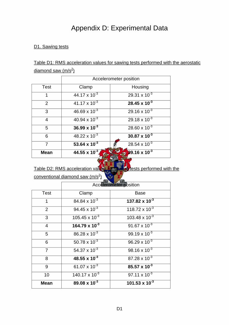
Appendix D: Experimental Data
D1. Sawing tests
Table D1: RMS acceleration values for sawing tests performed with the aerostatic
diamond saw (m/s2)
Accelerometer position
Test Clamp Housing
1 44.17 x 10⁻³ 29.31 x 10⁻³
2 41.17 x 10⁻³ 28.45 x 10⁻³
3 46.69 x 10⁻³ 29.16 x 10⁻³
4 40.94 x 10⁻³ 29.18 x 10⁻³
5 36.99 x 10⁻³ 28.60 x 10⁻³
6 48.22 x 10⁻³ 30.87 x 10⁻³
7 53.64 x 10⁻³ 28.54 x 10⁻³
Mean 44.55 x 10⁻³ 29.16 x 10⁻³
Table D2: RMS acceleration values for sawing tests performed with the
conventional diamond saw (m/s2)
Accelerometer position
Test Clamp Base
1 84.84 x 10⁻³ 137.82 x 10⁻³
2 94.45 x 10⁻³ 118.72 x 10⁻³
3 105.45 x 10⁻³ 103.48 x 10⁻³
4 164.79 x 10⁻³ 91.67 x 10⁻³
5 86.28 x 10⁻³ 99.19 x 10⁻³
6 50.78 x 10⁻³ 96.29 x 10⁻³
7 54.37 x 10⁻³ 98.16 x 10⁻³
8 48.55 x 10⁻³ 87.28 x 10⁻³
9 61.07 x 10⁻³ 85.57 x 10⁻³
10 140.17 x 10⁻³ 97.11 x 10⁻³
Mean 89.08 x 10⁻³ 101.53 x 10⁻³
D1
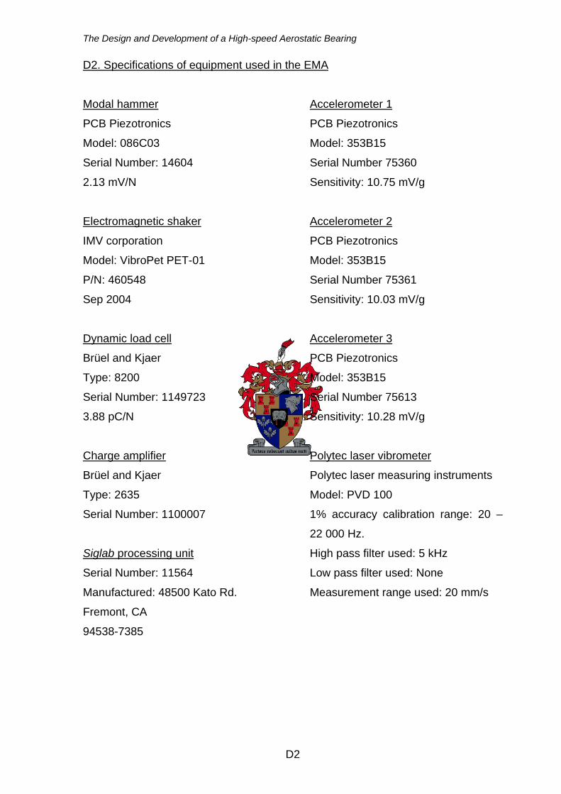
The Design and Development of a High-speed Aerostatic Bearing
D2. Specifications of equipment used in the EMA
Modal hammer
PCB Piezotronics
Model: 086C03
Serial Number: 14604
2.13 mV/N
Electromagnetic shaker
IMV corporation
Model: VibroPet PET-01
P/N: 460548
Sep 2004
Dynamic load cell
Brüel and Kjaer
Type: 8200
Serial Number: 1149723
3.88 pC/N
Charge amplifier
Brüel and Kjaer
Type: 2635
Serial Number: 1100007
Siglab processing unit
Serial Number: 11564
Manufactured: 48500 Kato Rd.
Fremont, CA
94538-7385
Accelerometer 1
PCB Piezotronics
Model: 353B15
Serial Number 75360
Sensitivity: 10.75 mV/g
Accelerometer 2
PCB Piezotronics
Model: 353B15
Serial Number 75361
Sensitivity: 10.03 mV/g
Accelerometer 3
PCB Piezotronics
Model: 353B15
Serial Number 75613
Sensitivity: 10.28 mV/g
Polytec laser vibrometer
Polytec laser measuring instruments
Model: PVD 100
1% accuracy calibration range: 20 –
22 000 Hz.
High pass filter used: 5 kHz
Low pass filter used: None
Measurement range used: 20 mm/s
D2