the derive - newsletter #87 user group - austromath

THE DERIVE - NEWSLETTER #87 ISSN 1990-7079

T H E B U L L E T I N O F T H E

U S E R G R O U P C o n t e n t s: 1 Letter of the Editor 2 Editorial - Preview Guido Herweyers 3 Statistics with TI-Nspire (3) 11 Surfaces from the Newspaper (7) Josef Böhm 12 Overcoming Branch & Bound by Simulation 38 User Forum Two hints for TI-NspireCAS A special sequence – a challenge for DUG members Eigendecomposition of a matrix

September 2012

D-N-L#87

I n f o r m a t i o n D-N-L#87

Unser DUG-Mitglied Johannes Zerbs ersucht um Bekanntgabe seiner Mathe Chilled Website. Dieser Bitte komme ich gerne nach. Was besonders bemerkenswert ist: Es handelt sich hier um kein kommerzielles Angebot! Ja, so was gibt es auch noch, Josef.

Mathe Chilled- ein Online Mathe Buch: Ein Rätselblock nach den neuesten Standards und Kompetenzen

www.mathe-chilled.at Gestern Mathe. Heute Mathe Chilled. Morgen in Mathe chillen....

As TIME Goes by …

Past TIME and future TIME

The “Kissing Students” are one of the most famous landmarks of Tartu, hosting town of TIME 2012 (left).

View of the old town of Krems (right). Krems is the entrance to the Wachau which is surely the most romantic part of the Danube valley between the Blackwood Forest and the Black Sea. Krems will host TIME 2014. Here is the place where it all began in 1992 with the first DERIVE Conference.

D-N-L#87

L e t t e r o f t h e E d i t o r p 1

Liebe DUG-Mitglieder,

leider bin ich wieder einmal nicht rechtzeitig mit unserem Newsletter fertig geworden.

Einerseits war ich sehr mit anderen Aufgaben beschäftigt und andererseits war dieser DNL sehr zeitaufwändig. Die Über-setzung des Statistikartikels ging rasch von statten – ermöglicht durch die gute Kommunikation mit Guido Herweyers. Dage-gen brauchte mein eigener Branch & Bound-Beitrag viel Zeit bis er meinen Wünschen entsprach. Aber das war ein schöner Aus-flug in meine Lehrervergangenheit.

Piotr Trebisz hat den letzten Teil sei-ner Schneckenhausserie geschickt. Ein spannender Austausch von E-Mails ermög-lichte interessante Ergänzungen zur Dar-stellung seiner schönen konischen Spiral-flächen. Aus Platzgründen muss ich das für den nächsten DNL zurückstellen.

Auch Dietmar Oertel wartet schon lan-ge auf die Veröffentlichung seiner Arbei-ten an den Primzahlen und Taylorreihen. Ich ersuche auch ihn um Geduld. Sie sind „under construction“.

Noch kurz zur TIME 2012: Herzlichen Dank an die Organisatoren vor Ort, Marina und Eno samt ihrem Team an der Universi-tät Tartu, Estland. Großen Dank auch an alle Teilnehmer, die hervorragende Hauptvor-träge und hochklassige Lektionen angebo-ten haben.

Eine Reihe von Vortragenden hatte nicht die Absicht, ihre Beiträge zur Veröf-fentlichung in Journalen einzureichen. Sie haben ihre Papiere dem DNL zur Verfügung gestellt. Vielen Dank dafür.

Schließlich möchte ich noch besonders auf die Themen im User Forum aufmerksam machen. Sie finden zwei kurze Hinweise auf TI-Nspire-Funktionen und zwei Probleme, die auf unsere DUG-Mitglieder warten.

Ganz aktuell: gemeinsam mit der Donau Universität Krems wird ACDCA die TIME 2014 vom 1. – 5. Juli 2014 in Krems an der Donau veranstalten.

Dear DUG Members, unfortunately I am too late with this

newsletter once more. On the one hand I was busy with other

duties and on the other hand production of this DNL was very time consuming. Transla-tion of the statistics contribution was – thanks good communication with Guido Herweyers – quickly done. My own article on Branch & Bound took much time until it met my expectations – and during writing new ideas wanted to be realized … This was a nice trip back to my past as teacher.

Piotr Trebisz sent the last part of his snail shell series. An exciting email ex-change brought interesting additions to the representation of his beautiful conic spiral surfaces. Because lack of space I must leave this for the next issue.

Dietmar Oertel has also been waiting a long time for publication of his prime num-ber and Taylor series investigations. Please be patient. They are “under construction”.

Concerning TIME 2012: many thanks to the local organizers, Marina, Eno and their team at Tartu University, Estonia. Many thanks also to all participants and present-ers. We had excellent keynotes and great lectures.

Some presenters didn’t intend to sub-mit their full papers for publication in spe-cial journals. They provided their presenta-tions for the DNL. Thanks for this offer.

Finally I’d like to draw your attention to the User Forum. You will find two short notes on Nspire functionality and two prob-lems waiting to be tackled by DUG mem-bers.

Latest – great – news: The Danube Uni-versity Krems and ACDCA will organize TIME 2014 from 1 to 5 July 2014 in Krems, Lower Austria.

Viele Grüße, kindest regards

Download all DNL-DERIVE- and TI-files from http://www.austromath.at/dug/

p 2

E D I T O R I A L

D-N-L#87 The DERIVE-NEWSLETTER is the Bulle-tin of the DERIVE & CAS-TI User Group. It is published at least four times a year with a content of 40 pages minimum. The goals of the DNL are to enable the ex-change of experiences made with DERIVE, TI-CAS and other CAS as well to create a group to discuss the possibilities of new methodical and didactical manners in teaching mathematics.

Editor: Mag. Josef Böhm D´Lust 1, A-3042 Würmla, Austria Phone: ++43-(0)660 3136365 e-mail: [email protected]

Contributions: Please send all contributions to the Editor. Non-English speakers are encouraged to write their contributions in English to rein-force the international touch of the DNL. It must be said, though, that non-English articles will be warmly welcomed nonethe-less. Your contributions will be edited but not assessed. By submitting articles the author gives his consent for reprinting it in the DNL. The more contributions you will send, the more lively and richer in contents the DERIVE & CAS-TI Newsletter will be. Next issue: December 2012

Preview: Contributions waiting to be published Some simulations of Random Experiments, J. Böhm, AUT, Lorenz Kopp, GER Wonderful World of Pedal Curves, J. Böhm, AUT Tools for 3D-Problems, P. Lüke-Rosendahl, GER Hill-Encryption, J. Böhm, AUT Simulating a Graphing Calculator in DERIVE, J. Böhm, AUT Do you know this? Cabri & CAS on PC and Handheld, W. Wegscheider, AUT An Interesting Problem with a Triangle, Steiner Point, P. Lüke-Rosendahl, GER Graphics World, Currency Change, P. Charland, CAN Cubics, Quartics – Interesting features, T. Koller & J. Böhm, AUT Logos of Companies as an Inspiration for Math Teaching Exciting Surfaces in the FAZ / Pierre Charland´s Graphics Gallery BooleanPlots.mth, P. Schofield, UK Old traditional examples for a CAS – what’s new? J. Böhm, AUT Truth Tables on the TI, M. R. Phillips, USA Where oh Where is It? (GPS with CAS), C. & P. Leinbach, USA Embroidery Patterns, H. Ludwig, GER Mandelbrot and Newton with DERIVE, Roman Hašek, CZK Tutorials for the NSpireCAS, G. Herweyers, BEL Some Projects with Students, R. Schröder, GER Structures in the Set of Prime Numbers, D. Oertel, GER Dirac Algebra, Clifford Algebra, D. R. Lunsford, USA Laplace Transforms, ODEs and CAS, G. Picard & Ch. Trottier, CAN A New Approach to Taylor Series, D. Oertel, GER Cesar Multiplication, G. Schödl, AUT Henon & Co; Find your very own Strange Attractor, J. Böhm, AUT Rational Hooks, J. Lechner, AUT Mathematical Model for Snail Shells (4), P. Trebisz, GER Simulation of Dynamic Systems with various Tools, J. Böhm, AUT An APL-like SHAPE function in DERIVE 6, D. R. Lunsford, USA Brussels Gate in Dendermonde, E. van Lantschoot, GER and others

Impressum: Medieninhaber: DERIVE User Group, A-3042 Würmla, D´Lust 1, AUSTRIA Richtung: Fachzeitschrift Herausgeber: Mag. Josef Böhm

D-N-L#87

Guido Herweyers: Statistics with TI-Nspire 3.1 (3) p 3

Statistics with TI-Nspire 3.1/3.2 (Part 3) Visualising and Simulating Dynamically with TI-Nspire

Guido Herweyers, KHBO Campus Oostende [email protected]

Part 2: Simulating with TI-Nspire

(1) Generating random numbers

Open a calculator page. In the menu 5: Prob-ability > 4: Random can you find the com-mands for generating random numbers.

Click on Seed or type randseed followed by space. Then type any natural number in order to initiate a new series of random numbers.

Examples for generating random numbers (you may compare with the TI-84 Plus com-mands) are:

→ rand(): a real random number between 0 and 1. So gives 3 + 5 ⋅ rand() a random number within the interval (3,8).

→ rand(10): a list of 10 random numbers between 0 and 1.

→ randint(1,6): a natural number from 1 to 6 (throwing a die).

→ rand(1,6,20): a list of 20 integers within [1,6] (throwing a die 20 times).

→ randbin(10,0.5): the number of heads when throwing a coin 10 times.

→ randbin(10,0.5,20): a list of the results repeating “= TIMES the coin experiment from above.

→ randnorm(175,10): a normal distributed random number with mean = 175 and standard deviation = 10.

→ randnorm(175,10,50): a sample (list) of 50 random numbers from a normal distribution with mean = 175 and standard deviation = 10.

p 4

Guido Herweyers: Statistics with TI-Nspire 3.1 (3) D-N-L#87

(2) Samples with and without replacement A sample from a list of numerical or categorical data is taken using the command randsamp. Its syn-tax is: with replacement: randsamp(list name, sample size, 1) without replacement: randsamp(list name, sample size)

(You can find the roulette rules together with the win chances in http://www.casino-gids.be/artikels/spelregels/beginners/roulette.php.) The screen shown above was created in a Notes Application.

The output of a Maths Box used in a Notes Application can be shown or hidden. Perform a right mouse click in the Maths Box and choose the respective attributes. The lottery list {1,2, …, 44, 45} is hidden and the roulette list is shown.

The Notes Application is very useful. It is an elementary text processor combined with a dynamic calculator in an environment which enables easy quick repetitions of simulations.

• You are able to combine text and mathematical expressions (like in a calculator page). A mathe-matical expression is written in a Maths Box, which can be activated by pressing Ctrl + M. As shown above you can hide the result of the evaluation: right click on the Maths Box and then choose the Maths Box Attributes.

• The Notes Application is dynamic (in contrary to the static Calculator Application): changes of a definition result in an immediate recalculation of all expressions in the Notes.

• A simulation – which is an expression containing rand… in any form – is automatically reevalu-ated by clicking on the expression followed by ENTER (or by pressing Ctrl+ENTER in order to perform quick repetitions of the simulation). Unfortunately this does not work any longer in ver-sion 3.2. Here you need a respective column in the spreadsheet where you can repeat the simula-tion by pressing Ctrl+R. Read more about this on page 6.

D-N-L#87


Hint: Having defined a column in a spreadsheet application using a simulation command then the simulation is immediately reevaluated after clicking the spreadsheet and then pressing Ctrl+R.

Ctrl+R Ctrl+R

(3) Rolling two Dice We split the screen into three applications: Lists & Spreadsheet, Notes, and Data & Statistics. Sample size n and simulation sumd (sum of the two dice) are defined within the Notes. Spreadsheet and bar chart as well will change dynamically when performing a new simulation by changing the sample size n and by repeating the simulation or by clicking in the sumd Maths Box and then pressing ENTER. Investigate the influence of the sample size on the variability of the sample and the “convergence” to the theoretic probabilities of the sum of two dice.

It is really a pity that the full text in this paper is only static and not dynamical …

p 6


(4) Probability distribution of the sample mean In the following we will discuss the principle how to find an approximation for the probability model of the sample mean.

• Take a big number of samples from a population with a discrete or continuous probability distribution.

• Note for each sample its mean and append its value to a list via automatic capturing in a column of the spreadsheet application.

• A dot plot of the list shows whether the probability model of the sample means should be a discrete or a continuous one.

• Observe graphically the convergence of the percental distribution of the bar chart for a discrete model or the convergence of the density histogram (with small enough class widths) for a continuous model to a stable situation.

• The “equilibrium situation” gives an approximation of the probability distribution of the sample means.

For didactical reasons it is recommended to take the sample from a concrete given population of num-bers like the results of main part 4 of the life guards which is a population of 367 data showing a nega-tively (= left) skewed distribution (long lower tail).

This is much more realistic for the students than taking a sample from an artificial population which is generated by applying a probability model (e.g. the uniform distribution for rolling a die).

Introduce the data as shown below in the Notes. Sometimes it is necessary to execute a command with Ctrl+ENTER (instead of only ENTER) in order to get the result in decimal form (instead of a frac-tion). Examples for this are samplemean and mean(h4).

The mean of each sample will be automatically added to the list means, which has been defined in the spreadsheet application: click into the formula cell and call Data > Data Capture > Automatic in the Spreadsheet Toolbox, then change capture(var,1) to capture(samplemean,1).

For taking random samples provide a Maths Box (Ctrl+M) and type sample:=randsamp(h4,n). Another Math Box is necessary to calculate the samplemeans: samplemean:=mean(sample). These results are collected in the spreadsheet column means. To get a really good impression you need many samples, so keep pressing Ctrl+ENTER in the sample-Maths Box for repeating the process many times. Accomplish the Notes according to the screenshot given below … but …

… inspecting this screenshot you will find another column sample in the spreadsheet. Why this? Un-fortunately TI-Nspire changed its behaviour from Version 3.1 to 3.2 as mentioned on page 4 in such a way that pressing Ctrl+ENTER in the Maths Box does not repeat the simulation. You have to define the sample in a column. Then click into any cell of the spreadsheet and press Ctrl+R.

Perform a sufficient large number of samples.

Don’t forget to change the RandSeeds or ask the students to take different RandSeeds otherwise they could get identical results – and this is will not give a “random like” impression.

D-N-L#87


Working with sample size n = 4 we find the probability distribution of the mean less skewed than the populations’s one. You can see a simulation of 2055 samples. The average of all means is 64.98 which is very close to the mean of the population 65.00. The deviation is almost halved.

Sample size n = 16 and a series of simulation of 2251 samples. Deviation is halved again.

p 8


Sample size n = 64, 1382 samples. Sample is … Illustration of the Central Limit Theorem. The reader is invited to experiment with samples taken from other (discrete or continuous) popula-tions. This shall lead to the conjecture that the probability model of the sample mean population – on condition that the sample size is sufficient large – can be approximated by a bell-shaped model – the normal distribution.

The bell-shaped probability model of a normal distributed population is completely defined by its population mean µ and its standard deviation σ. The influence of these parameters on the graph of the density function will be investigated by introducing sliders.

How to achieve the screen given below? This is the answer:

• Split the page horizontally into a Graphs-application and a Notes-Application.

• Activate the Graphs and introduce four sliders via the Graphs & Geometry Toolbox: 1:Actions > B:Insert Slider. The Greek letters can be found among the Utilities in the Documents Toolbox.

(Take care that you take the right µ.

The µ-character shown in the first row is a system variable which cannot be used.)

Insert sliders for two means µ1, µ2 and two standard deviation σ1 and σ2.

D-N-L#87


• Define the functions f1(x) and f2(x) via the entry line which appears after clicking on the

>> symbol bottom left (version 3.1). In version 3.2 make a right mouse click on the graph page. 2:Hide/Show > 5: Show Entry Line.

• Define two points on the x-axis using Points & Lines > Point On in Graphs & Geometry Toolbox > 8:Geometry. Then press ESC for leaving this menu.

• Show the coordinates of these points via 1:Actions > 8:Coordinates and Equations.

• Switch to the Notes and define the variables a and b as shown below.

• Return to the Graphs-application, move the cursor to the x-coordinate of the first point (the word “text” appears). Make a right mouse click on it and choose in the appearing pop-up menu 6:Variables > 2:Link to > a. Now this point is linked with the variable a. Repeat this procedure for the second point linking its x-coordinate with variable b.

• Calculate the area under the graph of f2(x) between a and b using the Analyse Graph menu > 7:Integral. Click on the graph and then fix the two points as boundaries.

Hint: In the Calculator Application and in the Spreadsheet Application you have access to the Maths Operators. Go to Statistics > Distributions and there you will find a couple of probability distribu-tions offered with the normal distribution among them.

If X ~ N(µ,σ), then

→ normPdf(x,µ,σ) = f(x) with f being the normal density function

→ normCdf(a,b,µ,σ) = P(a ≤ x ≤ b) and

→ invnorm(a,µ,σ) = x with a = P(X ≤ x)

p 10


(5) Variability of samples in box plots It is worth while to observe the variability of the samples by generating box plots for samples follow-ing in a row.

When taking small samples then the box plots should vary very much and should also differ from the population box plot significantly. Increasing the sample size the box plots of samples following each other are differing less and less. The random generated box plots shall also become more and more similar to the population box plot.

Take again h4 (367 life guards data) as population and take random samples of sample size n.

Random generated box plots with version 3.1 (above) and version 3.2 (below).

Next DNL: Part 4: Discovering Probability Distributions

D-N-L#87

Surfaces from the Newspaper (7) p 11

It was in DNL#71/72 when I presented some surfaces whose equations I found in the FAZ (Frankfurter Allgemeine Zeitung) some time ago. One empty page in this DNL is reason enough to have another three solids with DPGraph (left) and DERIVE (right), Josef

p 12

Josef Böhm: Overcoming Branch & Bound D-N-L#87

Overcoming Branch & Bound by Simulation

Josef Böhm

When I was a teacher at the St.Pölten College for Business Administration (Handelsakademie) I had to teach several years “Planungsmathematik” which is a possible German word for Operations Research. This was in the early 70ties. The curriculum covered topics as Linear Programming, Critical Path Methods, and heuristic methods as Branch & Bound. Using Branch & Bound we solved Travelling Salesman problems, Knapsack problems and Assignment problems. Very small problems can be solved by complete enumeration, i.e. trying all possible combinations and checking them for validity and for leading to a maximum or minimum of the given goal function.

All these problems are NP hard (they have no polynomial algorithm for solving). Bigger problems become very time consuming.

Branch and Bound (B&B) is by far the most widely used tool for solving large scale NP-hard combinatorial optimization problems. B&B is, however, an al-gorithm paradigm, which has to be filled out for each specific problem type, and numerous choices for each of the components exist. Even then, princi-ples for the design of efficient B&B algorithms have emerged over the years[*].

Guido Herweyers explains simulation performed with TI-Nspire. So I believe that it might be a good idea to demonstrate applying simulation for solving the problems mentioned above by simulation.

1 The Travelling Salesman Problem (Rundreiseproblem)

Given a set of locations, and known distances between each pair of loca-tions, the Travelling Salesman Problem is the problem of finding a tour that visits each location exactly once and that minimises the total distance trav-elled.

Let’s start with 5 towns. The distances are given in the table below. The matrix needs not to be sym-metric.

A B C D E

A – 5 10 6 7

B 5 – 8 8 5

C 10 8 – 8 5

D 6 8 8 – 7

E 7 5 5 7 –

It needs 5 miles from A to B, 10 miles from A to C, etc. We will find the shortest trip starting in A visiting all other places and then returning to A.

Route A-B-C-D-E-A would be 35 miles. [1] http://www.diku.dk/OLD/undervisning/2003e/datV-optimer/JensClausenNoter.pdf

http://www.informatik.uni-trier.de/~ley/db/indices/a-tree/c/Clausen:Jens.html http://citeseerx.ist.psu.edu/viewdoc/summary?doi=10.1.1.5.7475

D-N-L#87

Josef Böhm: Overcoming Branch & Bound p 13

We could do it in the enumerative way and check all possible ( 1)! 12

2n −

= roundtrips in our case. This

is not so bad, but thinking on 20 cities to be visited gives 60822550204416000 possible tours! So enumeration is not the best choice to find a solution.

Question for students: Why are there ( 1)!2

n − different routes possible?

You can find a lot of materials about algorithms to tackle this classic problem. Among the heuristic methods you will meet the Branch & Bound Method. I will present this method later.

Now my idea is as follows: I generate a series of random tours (= random permutations of the loca-tions), calculate the respective mileage (cost, …) and then select the tour with the minimum value. Finally I will apply statistic means for estimating the quality of the “solution” which is in fact only an approximation.

My DERIVE approach:

I produce a random permutation of the “towns”:

As I am missing the useful randsamp-command which is available for TI-Nspire I took the chance to define a randperm()-function for DERIVE. (See also page 31.)

p 14


But for now I will proceed on my travel route. I append the starting point because I have to finish the roundtrip and calculate the mileage which is again 35. Is this the shortest roundtrip?

It would be very boring to do this one route after the other. The solution is collecting all steps in one program:

I didn’t include simul in the parameter list because it is a global variable which is necessary for my intention. p, cost, way, and dummy are local variables.

This is my first run of the program performing 5 simulations. Of course, It can happen that tours are appearing twice or even more often.

The first route is the shortest one with length 29.

We can assume that the lengths L of the routes follow a normal distribution[1]. First we calculate mean and standard deviation of the sample and then the probability p(L ≤ 29).

There is a probability of only 4% to find a better solution, i.e. a shorter route combining all towns.

A sample of size 5 is too small. I increase the number of simulations 1000 random routes.

D-N-L#87


When evaluating expression #19, the resulting matrix (1000 rows) is stored as global variable simul. I need simul for determining mean and standard deviation of the route lengths. If we would not take simul in #21 but run1 instead then a new simulation would be performed. If you try dim(simul)= you will get immediately 1000 but when simplifying dim(run1)= it will need some time to first per-form internally the next 1000 simulations and then show the number of rows = 1000.

The probability to find a better solution has decreased to 2.5% which is pretty good.

There are 87 routes with minimal length 87 which need not be all the same. I’d like to see the first three of them and am finding out that they all are the same. Maybe that there is at least one another one among the remaining 84 solutions. But we cannot be absolutely sure that 29 is the shortest possi-ble route. It remains an approximation.

Selecting the minimum together with returning the optimal route could also be included into the pro-gram travel. I did without in the first application but I will do this for the other problems.

You will see that my programming style will improve stepwise. This could also be done with students. I remember that at similar occasions the students had ideas what should – and often really could – be improved

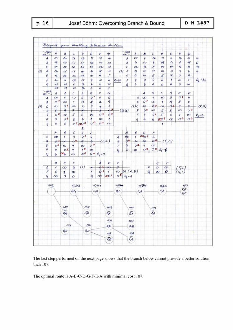
Let’s have a problem with more locations. This is a problem I used as teacher demonstrating the Branch & Bound Method. As I said above this was in the early 70ties. I will show my original “prepa-ration” provided for the classroom, doing all calculations by hand. The distance matrix – which is now defined as a cost matrix – is not symmetric and there are 7 locations.

p 16


The last step performed on the next page shows that the branch below cannot provide a better solution than 107. The optimal route is A-B-C-D-G-F-E-A with minimal cost 107.

D-N-L#87


The DERIVE procedure:

The selection of all routes with a given value (107) is done by a function sel(val). Comparing with my solution found in the last century we can see the correspondence.

p 18


The probability of 0.5% finding a shorter path is sufficiently small to accept 107 miles at least as a good approximation – even without knowing the exact result – as we do here.

Finally let me show a more extended travel route as given in [2]:

This is the map with the distances between villages A to M. We need to find the shortest path connect-ing all places starting and ending in town A.

The first problem is to find out the shortest connections in pairs be-tween all villages – considering all nodes. We will assume that this problem has been solved for using a special algorithm (Dantzig).

The distance matrix trm is given.

D-N-L#87


11 villages give 1 814 400 possible routes. Which of them is the shortest one? I run three time 10000 simulations:

The best result is 104.5 miles. Calculation gives a very small chance to find a better one.

Starting in A the route is: A – F – D – C – B – E – J – H – L – K – G – M – A.

Preparing the DNL I tried once more hoping to find a better approximation:

The approximation given in [2] is much better. After some pages following a tiresome algorithm the approximation leads to a total distance of 84.1 when using the route A-B-C-D-F-E-J-H-K-L-G-M-A.

The first figure shows the graph connected with the route length 104.5.

p 20


The next one gives the route with total length 84.1.

Even be inspection we recognize that this is a much better solution. So we would need more simula-tions to obtain a shorter path? Maybe that we would be lucky with the next single simulation. The reader is invited to follow the route with length 100.1.

The Travelling Salesman problem tackled with the TI-92 / Voyage 200:

D-N-L#87


As you can see it works pretty well.

The route produced by this simulation (50 tries) gives the optimal solution.

I tried the second problem – with 7 locations:

Not so bad!! [1] Autorenkollektiv, Mathematische Standardmodelle der Operationsforschung, Verlag Die

Wirtschaft Berlin 1972.

[2] Autorenkollektiv, Mathematische Standardmodelle der Operationsforschung, Aufgabensamm-lung, Verlag Die Wirtschaft Berlin 1972.

http://en.wikipedia.org/wiki/Travelling_salesman_problem

http://de.wikipedia.org/wiki/Problem_des_Handlungsreisenden

http://www.tsp.gatech.edu/

http://mathworld.wolfram.com/TravelingSalesmanProblem.html

http://www.lancs.ac.uk/staff/letchfoa/talks/TSP.pdf

http://elib.zib.de/pub/UserHome/Groetschel/Spektrum/index2.html

p 22


2 The Assignment Problem (Zuordnungsproblem)

There are a number of agents and a number of tasks. Any agent can be assigned to perform any task, incurring some cost that may vary depending on the agent-task assignment. It is required to perform all tasks by assigning exactly one agent to each task in such a way that the total cost of the assignment is minimized.

The cost matrix – 6 projects are to be assigned to 6 agents is given by:

We can also interpret the matrix as a profit matrix because the agents perform their tasks more or less efficient. Then the maximum assignment is required. My program assign(matrix, number of simulations) is looking for minimum and maximum as well.

Additionally I have included all steps leading to the final answers (fixing min and max, selecting the respective assignments and providing a nicely formatted output of the results).

D-N-L#87


Having performed 10 simulations which will very likely not give good approximations, I will try 2000 randomly chosen assignments. This needs only 9.7 seconds:

This is much better now.

The probabilities to find better solutions are very small.

Here is a second example from the 70ties-textbook. Seven jobs shall be assigned to seven machines.

The cost/profit-matrix is given by:

Looking back to my 40 years old papers I see that there are more optimal assignments possible. This reminiscence gives the opportunity for demonstrating the Branch & Bound method once more.

p 24


We see that the manual procedure gives four solutions for the minimum problem – and there are two solutions for the maximum problem. I changed my program assign in order to return not only one solution – but I cannot be sure that we will find all possible solutions.

D-N-L#87


This took me 228 seconds. Comparing with my papers from the past, I can say that all optimal as-signments for minimum and maximum as well have been found by simulation. Look at the probabili-ties!

http://faculty.ksu.edu.sa/jkhan/Documents/OR/opt-lp5.pdf

http://cse.spsu.edu/bmorrison/cs4413_ppt/branch&bound.ppt

Josef, Karsten Schmidt and Carl Leinbach (Tartu 2012)

p 26


3 The Knapsack Problem (Rucksackproblem)

Given a set of items, each with a weight and a value, determine the number of each item to include in a collection so that the total weight is less than or equal to a given limit and the total value is as large as possible. It derives its name from the problem faced by someone who is constrained by a fixed-size knapsack and must fill it with the most valuable items.

Example:

Let’s assume there is a burglar. He finds 6 items worthwhile to take them. They differ in weight and value. He is able to carry not more than 65 pounds. What is his best choice?

Item i A1 A2 A3 A4 A5 A6

Weight wi 30 20 8 25 12 15

Value vi 25 18 10 20 15 8

There is a recursive algorithm. The respective recursion formula is given by:

( 1, )( , )

max( ( 1, ), ( 1, ))k k

f k gf k g

v f k g w f k g−

= + − − −

ifif and 0

k

k

w gw g k

>≤ >

The last values are k = n (which is 6 in our case, and g = M = 65).

The result of the procedure should be f(6,65) = 63.

D-N-L#87


See three series of simulations followed by the original binary B & B from my OR-teaching.

p 28


This is a so called (0,1)-problem: Take it (= 1) or do not (= 0). So we have 26 possible choices from (0,0,0,0,0,0) – leave all items – to (1,1,1,1,1,1) – take them all. It is left to the reader to write an enu-merative procedure to check all possibilities (= end of all branches) for validity (total weight not more than 65 pounds) and for maximal total value.

I transferred the Travelling Salesman problem to the TI-92 / Voyage 200. Now I will tackle the Knap-sack problem with TI-NspireCAS.

The problem is from my old textbook again. It is a really “Knapsack = Rucksack” problem:

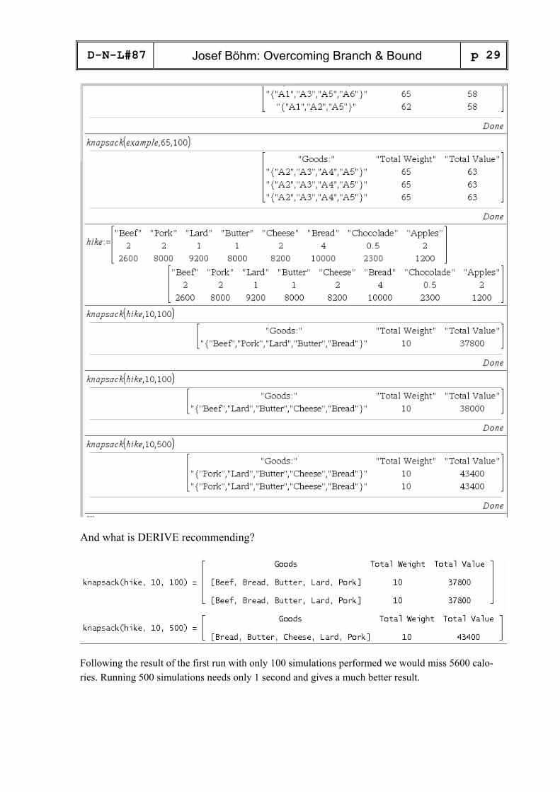
A hiker packs his rucksack. He can to choose between eight victuals.

The second row gives the weight (kg), the third one shows the calorie content. The hiker doesn’t want to carry more than 10 kg.

Find the selection with maximum calorie content under the condition that the eatables are indivisible.

This is the TI-Nspire program:

D-N-L#87


And what is DERIVE recommending?

Following the result of the first run with only 100 simulations performed we would miss 5600 calo-ries. Running 500 simulations needs only 1 second and gives a much better result.

p 30


I found in Müller-Merbach[1] an economic application: An investor wants to invest 1300 monetary units (say 1000 €). He has the choice of 7 indivisible investments with different returns of investment (also given in 1000 €). How should he put together his portfolio?

Our recommendation is: buy stocks A, C, E, F and G and make a profit of 93 000 €!!

D-N-L#87


[1] Müller-Merbach, Operations Research, Vahlen 1971 [2] The Operations Research Problem Solver, REA, New York 1985 http://www.diku.dk/users/pisinger/95-1.pdf http://en.wikipedia.org/wiki/Knapsack_problem http://www.es.ele.tue.nl/education/5MC10/Solutions/knapsack.pdf http://www.diku.dk/users/pisinger/95-1.pdf http://www.nuigalway.ie/mat/algorithms/knapsack.html (a program!!) http://www.cs.ucsb.edu/~jacopo/BB/ (a Branch & Bound Solver)

I’d like to add two comments: (1) I really like to undertake extended hikes. But I never had the idea to carry lard with me. It

might be difficult enough to have butter in the rucksack climbing up a mountain on its sunny side in summer time …. And I never had beef and pork with me. And why should I not be able to divide butter, bread, cheese, …? Believe it or not this is the original text from the textbook.

(2) I also like programming and exploring the advantages and disadvantages of various program-ming languages and various programmable computer algebra systems. I missed Nspire’s randSamp function. So what to do? Easy answer: make your own DERIVE randSamp-function and benefit from DERIVE’s feature to implement “real” random processes without needing a “randseed” using its RANDOM(0) command.

4 randSamp & co

Let’s start with a random permutation of n elements. I wantd to avoid simplifying RANDOM(0) at the beginning of each session so I included this command in the function in order to have every time an-other initial value for the random number generating process.

This looked pretty good. I proceeded with a sequence of three random permutations of the set test in a row.

I was very disappointed that the same permutation is appearing three times!

p 32


Ok, I’ll come back to this problem later. We wanted to have random samples – with and without re-placement (of the elements).

The same problem as above occurred. One function call after the other worked properly, a sequence of random samples seemed not to be really randomly!! randsamp(population,n) generates a sample of n elements with repetition by default). Including 1 as third parameter avoids repetition of elements in the sample.

Do you know the reason for the repeated samples? I believe to know. The CPU works too fast. RAN-DOM(0) uses the internal CPU time as initial value for the random number generating algorithm. And it seems to be that this time does not change between two or even more calls of the function. What to do is, giving the machine some time for “thinking” or doing some useless work:

I let DERIVE count from 1 to 100 in the last loop. Counting only to 10 or 20 is not sufficient (I tried).

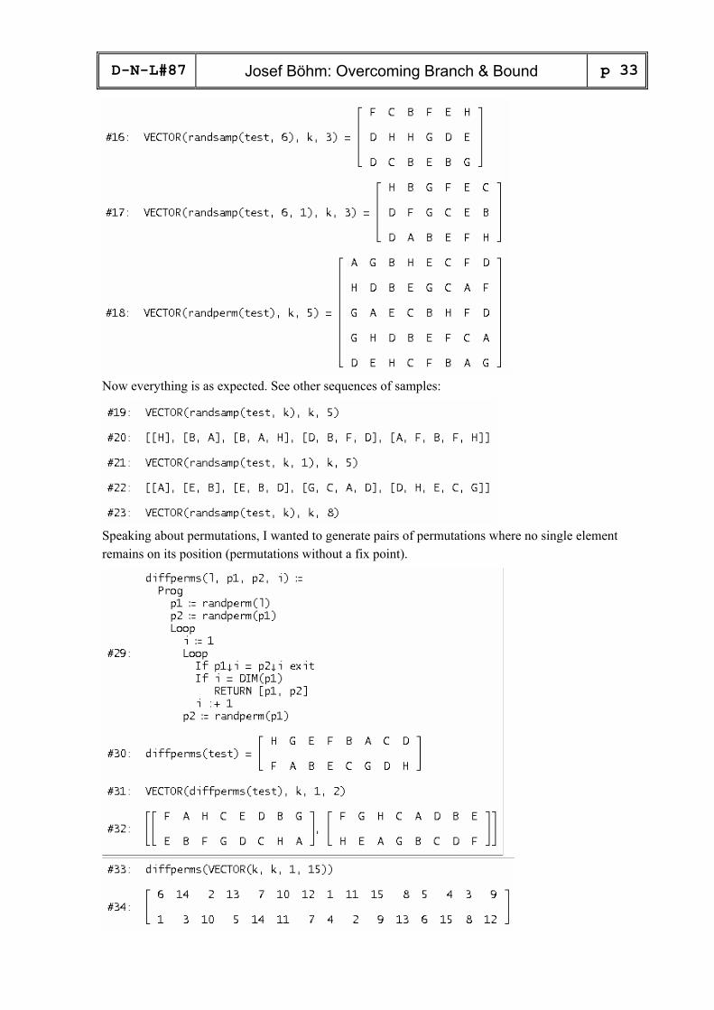
I can use randsamp to produce a random permutation, too, because this is only a special case (taking a sample of all elements without replacement).

I try again generating a sequence of samples and permutations:

D-N-L#87


Now everything is as expected. See other sequences of samples:

Speaking about permutations, I wanted to generate pairs of permutations where no single element remains on its position (permutations without a fix point).

p 34


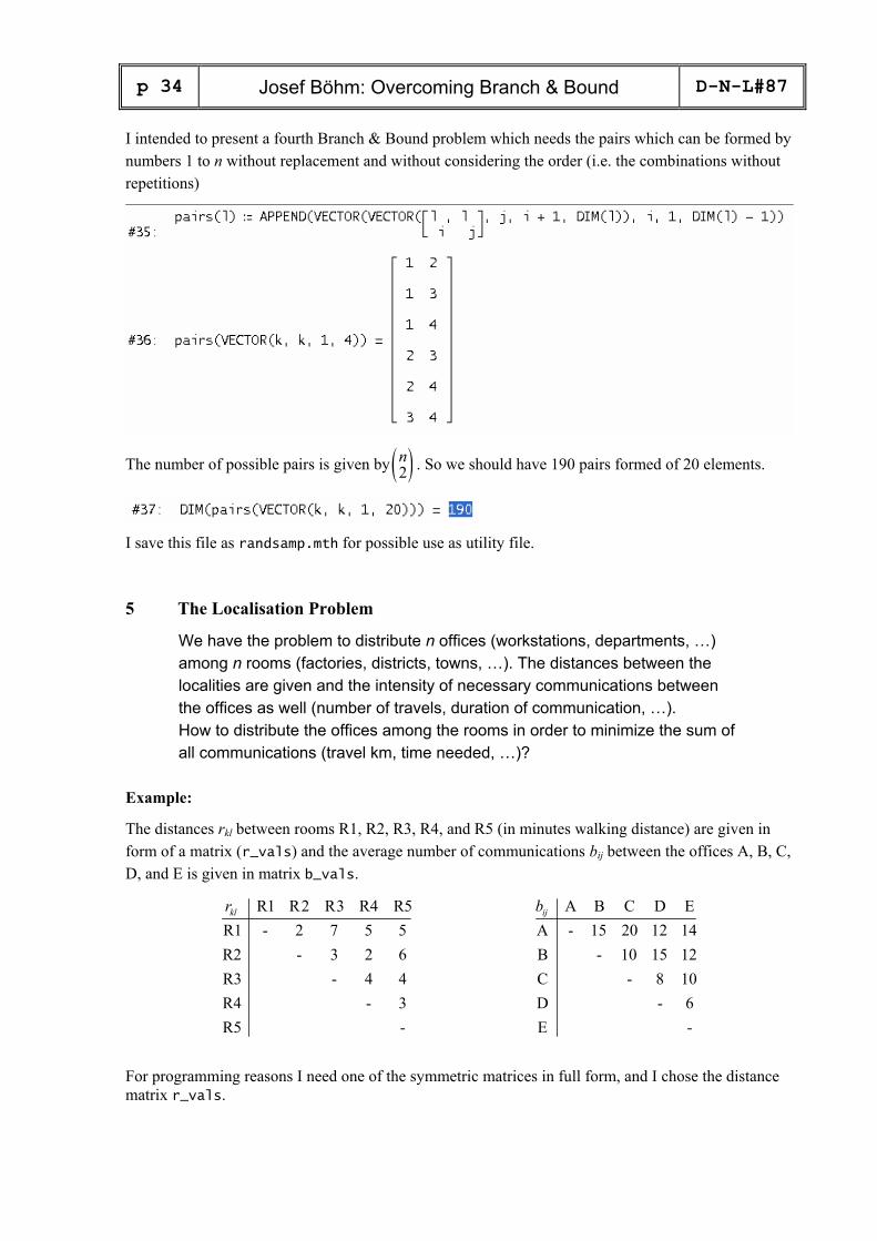
I intended to present a fourth Branch & Bound problem which needs the pairs which can be formed by numbers 1 to n without replacement and without considering the order (i.e. the combinations without repetitions)

The number of possible pairs is given by ( )2n . So we should have 190 pairs formed of 20 elements.

I save this file as randsamp.mth for possible use as utility file.

5 The Localisation Problem

We have the problem to distribute n offices (workstations, departments, …) among n rooms (factories, districts, towns, …). The distances between the localities are given and the intensity of necessary communications between the offices as well (number of travels, duration of communication, …). How to distribute the offices among the rooms in order to minimize the sum of all communications (travel km, time needed, …)?

Example:

The distances rkl between rooms R1, R2, R3, R4, and R5 (in minutes walking distance) are given in form of a matrix (r_vals) and the average number of communications bij between the offices A, B, C, D, and E is given in matrix b_vals.

R1 R2 R3 R4 R5R1 - 2 7 5 5R2 - 3 2 6R3 - 4 4R4 - 3R5 -

klr

A B C D EA - 15 20 12 14B - 10 15 12C - 8 10D - 6E -

ijb

For programming reasons I need one of the symmetric matrices in full form, and I chose the distance matrix r_vals.

D-N-L#87


Read this matrices as follows:

15 communications between A and B if A is located in room 1 and B in room 3 will need totally b12⋅r13 = 15 ⋅ 7 = 105 minutes, but if A and B were located in rooms 5 and 3 then the time needed for walking between A and B would be b12⋅r53 = 15 ⋅ 4 = 60 minutes, etc.

For understanding my program let’s assume that the present distribution is given by:

Offices A B C D ERooms R3 R4 R2 R1 R5

All necessary walks sum up as follows to 467 minutes.

12 34 13 32 23 14 31 13 15 35

23 24 24 14 25 45

34 12 35 25

45 15

(A,B) (R3,R4) (A,C) (R3,R2) (A,D) (R3,R1) + (A,E) (R3,R5)

15 4 10 3 12 7 14 4 230

10 2 15 5 12 3 131

8 2 10 6 76

6 5 30

467

b r b r r b r r b r

b r b r b r

b r b r

b r

⋅ + ⋅ + ⋅ ⋅⋅ + ⋅ = + ⋅ = + ⋅⋅ + ⋅ + ⋅ + ⋅ =

⋅ + ⋅ + ⋅⋅ + ⋅ + ⋅ =

⋅ + ⋅⋅ + ⋅ =

⋅⋅ =

Now you can recognize the purpose of the list of pairs (named co in the following program).

I preload randsamp.mth as utility file to use randperm and pairs as well.

The core line for finding the sum as described above is given by cost:=….

p 36


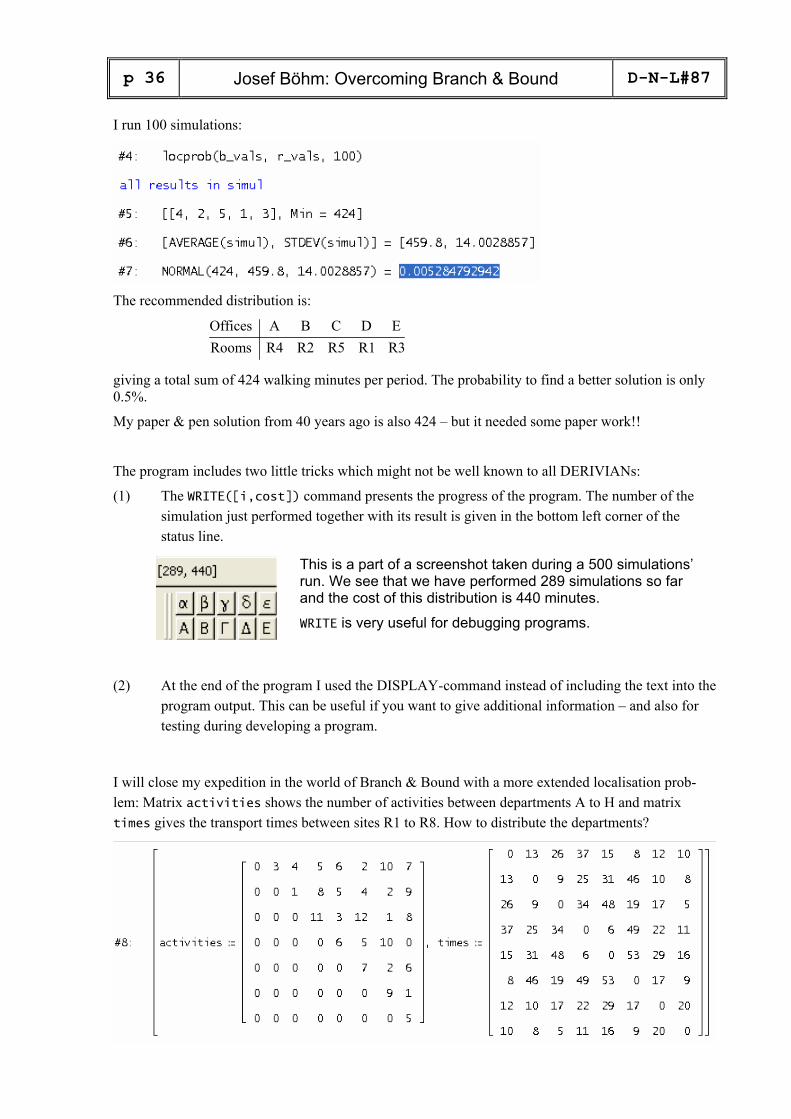
I run 100 simulations:

The recommended distribution is:

Offices A B C D ERooms R4 R2 R5 R1 R3

giving a total sum of 424 walking minutes per period. The probability to find a better solution is only 0.5%.

My paper & pen solution from 40 years ago is also 424 – but it needed some paper work!!

The program includes two little tricks which might not be well known to all DERIVIANs:

(1) The WRITE([i,cost]) command presents the progress of the program. The number of the simulation just performed together with its result is given in the bottom left corner of the status line.

This is a part of a screenshot taken during a 500 simulations’ run. We see that we have performed 289 simulations so far and the cost of this distribution is 440 minutes.

WRITE is very useful for debugging programs.

(2) At the end of the program I used the DISPLAY-command instead of including the text into the program output. This can be useful if you want to give additional information – and also for testing during developing a program.

I will close my expedition in the world of Branch & Bound with a more extended localisation prob-lem: Matrix activities shows the number of activities between departments A to H and matrix times gives the transport times between sites R1 to R8. How to distribute the departments?

D-N-L#87


My approximation is:

Departments A B C D E F G HLocalities R4 R2 R6 R8 R7 R1 R5 R3

with a minimal amount of time which is 2611 time units. (You may double check the result!)

There is tiny probability of 0.2% to find a better way to distribute the departments, so we are pretty fine with the result.

I had much pleasure doing all the programming and I am quite sure that there are some ways to improve the procedures. I would like to invite you to improve the programs and to provide other B & B methods for simulation.

Many DUG members in front of the Kissing Students on the town square of Tartu (above). Part of the TIME 2012 social program: Learning and practising counting in Estonian (right).

p 38

User Forum D-N-L#87

Comment on “Circles in a Point” (DNL#86) Lieber Herr Böhm, vielen Dank für die neue Ausgabe des DNL! Besonders gelungen finde ich diesmal den Artikel „Points in a Circ-le“ von Roland Schröder. Bei der Anpassung der Lösung für die TI-Nspire-Software haben Sie mangels VECTOR-Befehl eine andere Lösung vorgeschlagen. Mit dem Nspire-Befehl constructMat lässt sich Herrn Schröders Vorge-hensweise jedoch weitgehend identisch übertragen: Many thanks for the new DNL issue. In particular I liked Roland Schöder’s contribution on “Points in a Circle” very much. Adapting the solution for TI-Nspire you proposed another approach because you missed the VECTOR command. But by applying the Nspire command constructMat it is possible to transfer Roland’s procedure nearly identical.

Herzliche Grüße / Best regards Jürgen Wagner, DUG Member since 1992 The Tribonacci Sequence with TI-Nspire In DNL#86 I did not use recursion for producing this sequence with TI-NspireCAS because I thought that this would be impossible – and I complained in Tartu about the lack of recur-sion. But Michel Beaudin gave a very valuable advice how to perform a recursion:

Many thanks to Michel. It is my pleasure to revise my opinion. Recursion is possible, Josef.

D-N-L#87

User Forum p 39

DERIVE 4 for DOS on HP 200LX

Minh Nguyen [mailto:[email protected]]

Hi, I am looking for derive 4 for dos to run on my HP 200LX. you know where i can get this now? Can’t find it anywhere. Much appreciated. Thanks

Two problems provided by Fred Tydeman and Karsten Schmidt

Problem 1: Non Recursive Definition

Fred Tydeman wrote on 11 August 2012: I have a set of values and two recursive definitions:

(1) 0(2) 2*0 1 1*1 1(3) 3*1 1 2*1 2*(1 0) 2(4) 4*2 1 3*3 3*(2 1) 9(5) 5*9 1 4*11 4*(9 2) 44(6) 6*44 1 5*53 5*(44 9) 265

...

...

ffffff

== + = == − = = + == + = = + == − = = + == + = = + =

The generalisation reads as follows:

( ) * ( 1) ( 1) ; (1) 0or

( ) ( 1)*( ( 1) ( 2)); (1) 0, (2) 1

nf n n f n f

f n n f n f n f f

= − + − =

= − − + − = =

Is there some way to get a non-recursive definition? His comment on 12 August was: Thanks to all that responded. They used either Maple or MATHEMATICA to solve this.

No one used DERIVE.

In looking at the various solutions sent to me, I came up with this:

!( ) nf ne

= , rounded to the nearest integer.

This should be a challenge for the DERIVIANs – and the “Nspirians” as well to tackle this problem!

p 40

User Forum D-N-L#87

Problem 2: Eigendecomposition

… and for this I need the eigendecomposition (spectral decomposition = Spektralzerlegung) of a symmetric matrix: Let A a symmetric matrix. Then A = Q⋅L⋅Q´. L is a diagonal matrix with the eigenvalues of A in the main diagonal and Q is the orthogonal matrix of the eigenvectors of A (see rule 4.1.11 in our Springer textbook[1]). Do you know if anybody has done this with DERIVE before? This is, you know, very tiresome to write the eigenvalues into the main diagonal of a diagonal matrix. (The eigenvalues can appear multi-ple, i.e. the number of them which are returned by the EIGENVALUES function can be too small.) And it is much more laborious to calculate the respective eigenvectors using the EX-ACT_EIGENVECTORS-function, scale them to length 1, and then write them into matrix Q. Best regards Karsten Schmidt I am no matrix algebra specialist at all. I took Karsten’s textbook and studied carefully rule 4.1.11 presenting the spectral decomposition of a 2x2 matrix together with the following ex-ample 9. I wanted to apply this decomposition on a 3x3 example. On the web I found (I don’t know which CAS was used): Example: Spectral Decomposition of a Correlation Matrix[2]

C <- matrix(nrow=3, ncol=3, data=0.5) C[1,2] = C[2,1] <- 0.7 C[2,3] = C[3,2] <- 0.9 diag(C) <- 1 print(C) gives [,1] [,2] [,3] [1,] 1.0 0.7 0.5 [2,] 0.7 1.0 0.9 [3,] 0.5 0.9 1.0 Eigenvalue Decomposition: sz <- eigen(C) # matrix of eigenvectors Gamma <- sz$vectors # diagonal matrix of eigenvectors Lambda <- diag( sz$values ) # test, if it results as C again test <- Gamma %*% Lambda %*% t(Gamma) print(test) gives [,1] [,2] [,3] [1,] 1.0 0.7 0.5 [2,] 0.7 1.0 0.9 [3,] 0.5 0.9 1.0

D-N-L#87

User Forum p 41

I was curious and wanted to know if I were able to reproduce this with DERIVE, too. This is how I did: First of all I tried to find a DERIVE function like diag(row vector) from TI-Voyage 200 and TI-NspireCAS to make the procedure easier.

My first surprise was that the scaled vectors w1, w2 and w3 were approximated to empty vectors (#6). Then I simplified the expression [w1:= …] and received a huge expression full of roots and trigonometric expressions (the solutions of the characteristic equation which is here a cubic). Then I approximated the exact result (resulting on #7) and built up the matrix of the scaled eigenvectors (= Q). It is possible to form the matrix and its transpose in exact mode, too, but …

Following Karsten’s rule matrix Q should be an orthogonal matrix, i.e. the product of Q and Q` should result in the 3x3 identity matrix.

p 42

User Forum D-N-L#87

I tried simplifying Q⋅Q` but I could not wait for the result, so I approximated the product and was pretty sure to receive the unity matrix (#11) – more or less approximated – as expected. Finally I performed the “test” from above using the approximated matrices only.

I had expected a result close to the given matrix A because of my numerical procedure, but – and this was my second, but positive surprise – the result was exact matrix A (in decimal form!). To be honest, if you increase the number of decimal places you will recognize that the result is rounded. This is the story of my first successful eigendecomposition of a symmetric matrix. [1] Schmidt, Trenkler, Einführung in die Moderne Matrix-Algebra, Springer 2006 I tried with TI-NspireCAS. I did not benefit from diag() only but also from the fact that eigVc(matrix) immediately returns the orthogonal matrix of eigenvectors. At the other hand TI-Nspire does not provide any exact results.

Karsten sent two additional DERIVE files: spectral2x2.dfw (treating example 9 from [1] spectral 3x3F (decomposition of a 3x3-matrix with multiple eigenvalues) http://www.stat.uni-muenchen.de/~chris/rkurs/Rkurs6.pdf http://www.ece.ucsb.edu/~roy/classnotes/210a/ECE210a_lecture15_small.pdf http://cseweb.ucsd.edu/~dasgupta/291/lec7.pdf

http://www.youtube.com/watch?v=hmahoeta4KY