the dangers of precipitous adjustment speed of recovery … · the dangers of precipitous...

The Dangers of Precipitous Adjustment Speed of Recovery Price tothe Closed-loop Supply Chain and Improvement Measure

LEI XIETianjin University

College of Management and EconomicsTianjin 300072

[email protected]

JUNHAI MATianjin University

College of Management and EconomicsTianjin 300072

[email protected]

Abstract: This paper analyzes the recycling price game in waste household appliance market in China. Basedon the analysis of recycling behavior game of two retailers and a manufacturer in closed-loop supply chain, wepropose that precipitous adjustment speed of recovery price will lead to the system go into a chaotic state. In thisstate, the recycling price of each recovery party will enter the chaotic state, and it will be significantly affectedby the initial price, the profit of each corporate will be apparent fluctuations, and thus the chaotic state caused bythe precipitous speed of price adjustment will make competition be invalid and vicious. In this regard, this paperintroduces delay decision-making to control the chaotic state and gives the Economics of chaos control.

Key–Words: supply chain, recycling household appliance, Nash equilibrium, chaos, delay decision

1 IntroductionReuse of resources, energy conservation, are impor-tant measures of the sustainable development strategy.The sustainable development strategy has become ahot topic. Today, the traditional supply chain addsthe reverse logistics process, to become a closed-loopsupply chain. The reverse logistics process is a pro-cess for product recycling. There are many things canbe recycled by reverse logistics, such as used batter-ies, used bottles, scrap metal and used household ap-pliances. Now in China, there has been the companyrecycling waste household appliances, such as TCLAOBO. Consumers can sell the used household appli-ances recycling companies to get some compensation.The recycling companies recycle the waste householdfrom the market while recycle it from retailers. Appli-ance recycling vendors can use reusable parts for re-production, in order to reduce production costs. Theycan also sell the useful parts to scrap material recy-cling market to get some benefits. Retailers play arole as recyclers in the recovery process, they earnthe difference of the price between manufacturer andthemselves. This paper will study the game complex-ity of appliance recycling market gradually developedin China.

Some people have done some research in the areaof appliance recycling. Adam D. Read [1] found theway to improve people’s awareness of recycling bystudying door-to-door household waste recycling inChelsea and other UK regions. Frans Melissen [2]

analysed the Dutch consumer several waste recyclingbehaviour and appliance recycling pilot program, anddraw some suitable measures to improve the recoveryof waste household appliances. Carsten Nagel [3] ad-vocated the use of reverse logistics to recycle IT prod-ucts. Carsten Nagel and Peter Meyer[4] establishedan EOL network model to analyze an electronics re-cycling company collection network in Germany. H.R. Krikke et al. [5] proposed a stochastic dynamicprogramming model for the largest net gain of prod-uct recovery. Zsolt Istvan et al. [6] studied reverse lo-gistics management system at the end electronic prod-ucts. Anna Nagurney and Fuminori Toyasaki [7] usedgenetic algorithm to analyze production and price oflogistics. Jae-chun Lee et al. [8] described the statusof the recovery of waste electrical and electronic inKorea.

The enterprises which participate in the processof reverse logistics, not only can contribute to envi-ronmental protection, but also can benefit from therecycling process. Therefore, there are more andmore studies about recycling channels and recyclingstrategy under different conditions, to get an optimalrecovery strategies and reasonable contract. Fleis-chmann [9] summarized reverse logistics activitiesfrom the reverse distribution, inventory control andproduct planning. Fleischmann [10] also investigatedthe product recovery reverse logistics network designof different sectors, summed up the composition oftypical reverse logistics network. Shih [11] studied

WSEAS TRANSACTIONS on MATHEMATICS Lei Xie, Junhai Ma

E-ISSN: 2224-2880 1 Volume 13, 2014

reverse logistics network model of Taiwan discardedappliances and computer, in a variety of recovery ratesand recovery produce conditions, determine the op-timal system by the mixed integer linear program-ming (MILP), to determine the number and positionof members involved in recycling network , and theservice area of each facility. Sheu [12] considered therecovery rate of waste products and the correspond-ing availability of subsidies from government orga-nizations, constructed multi-objective programmingmodel. Sun Zhihui et al. [13] analyzed price game inChinese cold rolled steel market and showed that howrelevant parameters cause chaos to occur and how tochange the relevant parameters to control the chaoticstate. Guo Yuehong [14] et al. established a collect-ing price game model for a closed-loop supply chainsystem with a manufacturer and a retailer, analyzedcomplex dynamic phenomena and the influences ofthe system parameters. Ma, J et al.[15] considereda three-species symbiosis Lotka - Volterra model withdiscrete delays and analyzed the influence of delays tolocal stability.

The structure of this paper is: The second part de-scribes the assumptions of this study, and a number ofsymbolic variables explanation, as well as the struc-ture of the model; the third part introduces the anal-ysis methods of the model; the fourth part describesthe occurrence of the chaos state and the adverse ef-fects of the chaotic state by numerical simulation; thefifth part describes the method to control chaos; andthe sixed part summarized.

2 Model Description

2.1 Model Framework

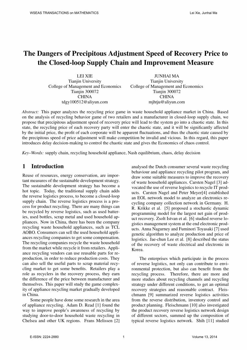
There are three main game parties in the appliance re-cycling market in the paper: appliance manufactur-ers, appliance retailers Gome and Suning. Retailersact as recyclers in the reverse logistics process of aclosed loop supply chain. Gome and Suning are thetwo largest home appliance retailers in China. Recov-ery amount they can obtain in the recycling processare so great that other small retailers cannot match.Therefore, the recovery process can be approximatedas a kind of oligopoly game. Manufacturers and retail-ers recover the waste products in the market as com-petitors. Manufacturer recovers waste products thatrecovered by the retailers and itself. The closed-loopsupply chain’s structure is shown in Fig.1 (solid linerepresents the forward supply chain, while dotted linerepresents reverse supply chain).

Figure 1: MR model closed-loop supply chain

2.2 Symbols and assumptions

First, give a description of symbols related in this pa-per:

i=1,2,3 represent manufacturer 1, retailer 2 andretailers 3, respectively.

qi: recovery amount obtained by recycling partyi in the market;

pi: recycling price of recycling party i;πi: profit of party i;γ, α and β: ratio that consumer willing to give

the waste products back to manufacturer 1, retailer 2and retailer 3, this variable is influenced by corporateimage of recycling party;

bi: price impact factor of the recycling amount,that is, the price elasticity of recycling;

ci and di: competitive factor, that is, the degreeof influence by other parties recycling prices;

ρ: recovery rate;Cm: the cost of a new product;Cr: remanufacturing costs of a recycling prod-

uct;Cb: disposal costs of a waste product;qs2 and qs3: sales volume of retailer 2 and retailer

3;Qs: sales volume of manufacturer, Qs=qs2+qs3;w: wholesale price of manufacturer 1;ps2 and ps3: sale price of retailer 2 and retailer 3.Based on the recycling amount model Guo Yue-

hong [14] proposed, the recycling amount model inthis paper can be written as model (1). The hypothet-ical scenario of this paper is that, the manufacturerand the two retailers recover the waste, manufacturerrecovers from retailers at a market recycling price.There is a price game between manufacturer and re-tailers in the recycling market. Recycling amountis influence by recycling price and corporate image,so the recycling amount consists of three parts: theamount that the consumer willing to give back, theamount influenced by its own price, the amount influ-enced by the other parties prices. In addition, the con-sumers have the same preference for the old products


E-ISSN: 2224-2880 2 Volume 13, 2014

and the new products.q1 = γ (qs2 + qs3) + b1p1 − c1p2 − d1p3q2 = α (qs2 + qs3) + b2p2 − c2p3 − d2p1q3 = β (qs2 + qs3) + b3p3 − c3p1 − d3p2

(1)

So the total amount on the chain is the sum of threesides recycling amount, that is Q = q1 + q2 + q3.

The profits of three vendors are shown in func-tion (2). Manufacturer’s profit is expressed as sellingnew products and the remanufacturing product, mi-nus the cost of production of new manufactured prod-ucts, minus available remanufacturing products pro-cessing costs, minus the payment cost of recovery pro-cess, minus the treatment cost of the recycled productwhich can not be reused.

Retailer’s profit consists of two parts, sales profitsand the price difference earned in the recycling pro-cess.

π1 = wQs − Cm (Qs − ρQ)− CrρQ− p1Q−Cb (1− ρ)Qπ2 = (ps2 − w) qs2 + (p1 − p2) q2π3 = (ps3 − w) qs3 + (p1 − p3)q3

(2)This paper studies the impact of recycling prices

on the corporate profits, therefore, it is necessary toconsider the marginal profitability of recycling price,that is, how many changes per unit change of recy-cling price can impact on the corporate profits. It isshown by function (3)

∂π1∂p1

= −Cb (b1 − c3 − d2) (1− ρ)

−ρ((2p1 −D) (b1 − c3 − d2) + (b2 − c1 − d3) p2+(b3 − c2 − d1) p3 + (α+ β + γ)Qs)

∂π2∂p2

= −αQs + p1 (d2 + b2)− 2p2b2 + c3p3∂π3∂p3

= −βQs + p1 (c3 + b3)− 2p3b3 + d3p3(3)

Model (4) is a cournot model, represents a priceadjustment model.

p1 (t+ 1) = p1 (t) + g1p1(t)∂π1(t)∂p1(t)

p2 (t+ 1) = p2 (t) + g2p2(t)∂π2(t)∂p2(t)

p3 (t+ 1) = p3 (t) + g3p3(t)∂π3(t)∂p3(t)

(4)

Three parties will determine the next phase of the re-cycling price based on their current marginal prof-its. When the marginal profit is positive, the higherprice will bring an increase in profits, so the corporatewill raise price. On the other hand, negative marginalprofit may lead to the fact that the lower price willbring an increase in profit, so the corporate will re-duce price. We introduce the concept of price adjust-ment factors: g1, g2 and g3. Price adjustment factorindicates the pace of price adjustment.

3 Model analysisTo further analyze the nature of the price adjustmentmodel to understand the game process of three partiesrecycling prices, we should find the equilibrium pointof the system and analyze the nature of the equilib-rium point.

3.1 Solving the equilibrium point

Under the condition of price stability, the threevendors’ prices will never change, so system haveachieved stable. In this state, the price will neverchange as time goes on. So we can use the follow-ing equation to express this state: pi (t+ 1) = pi (t).

The three parties profits for the second derivativeof the price function should be less than zero, in orderto ensure the highest profits are exist.

Solving equations (4), we can get eight group so-lutions

E1(0, 0, 0), E2(0, 0,−βQs

2b3), E3(0,−

αQs

2b2, 0),

E4(−(Cb(1− ρ)− dρ)m1 + ηQsρ

2m1ρ, 0, 0),

E5(0,−(2αb3 + βc2)Qs

4b2b3 − c2d3,−(2βb2 + αd3)Qs

4b2b3 − c2d3),

E6(e61, 0, e63), E7(e71, e72, 0), E8(e81, e82, e83).

where

e61 = [βm3Qs + 2b3(−Cbm1 −Qsη +m1ρCυ)]/

[(b3 + c3)m3 + 4b3m1]

e63 = −[(b3 + c3)(−βm3Qs − 2b3(−Cbm1

−Qsηm1ρCυ))]/[2b3((b3 + c3)m3 + 4b3m1)]

−βQs/2b3

e71 = [αm2Qs + 2b2(−Cbm1 −Qsη +m1ρCυ)]/

[4b2m1 + (b2 + d2)m2]

e72 = −[(b2 + d2)(−αm2Qs − 2b2(−Cbm1

−Qsηm1ρCυ))]/[2b2(4b2m1 + (b2 + d2)m2)]

−[αQs]/[2b2]

e81 = [(2b2m3 + c2m2)(2αb3 + βc2)Qs − (4b2b3

−c2d3)(αm3Qs + c2(m1Cb +Qs(α+ β + γ)

−m1ρ(Cb + Cm − Cr)))]/[(m3(b2 + d2)

−2c2m1)(−4b2b3 + c2d3) + (c2(b3 + c3)

+2b3(b2 + d2))(2b2m3 + c2m2)]

e82 = [(2αb3 + βc2)Qs]/[−4b2b3 + c2d3]

+[c2(b3 + c3) + 2b3(b2 + d2))((2b2m3

+c2m2)(−2αb3 − βc2)Qs + (4b2b3 − c2d3)

(αm3Qs + c2(m1Cb +Qs(α+ β + γ)

−m1ρ(Cb + Cm − Cr)))]/[(−4b2b3 + c2d3)


E-ISSN: 2224-2880 3 Volume 13, 2014

((m3(b2 + d2)− 2c2m1)(−4b2b3 + c2d3)

+(c2(b3 + c3) + 2b3(b2 + d2))(2b2m3 + c2m2))]

e83 = [(2b2β + αd3)Qs]/[−4b2b3 + c2d3]

+[2b2(b3 + c3) + d3(b2 + d2))(2b2m3

−c2m2(2αb3 + βc2)Qs + (4b2b3

−c2d3)(−αm3Qs + c2(−m1Cb −Qs(α+ β + γ)

+m1ρ(Cb + Cm − Cr)))]/[(−4b2b3

+c2d3)((m3(b2 + d2)− 2c2m1)(−4b2b3 + c2d3)

−(c2(b3 + c3)− 2b3(b2 + d2))(2b2m3 + c2m2)))]

To demonstrate this 8 groups of solution more clearly,we make

m1 = b1 − c3 − d2m2 = b2 − c1 − d3m3 = b3 − c2 − d1

(5)

The above 8 solutions are the 8 equilibrium points ofthe system.

3.2 Stability AnalysisNash equilibrium provides neither side will be ableto take the initiative to change in order to increaserevenue. When the profit margin is zero, increasingor decreasing the recovery price will result in loss ofprofits. Therefore, when each of the three vendorsprofit margin for the price is zero, the Nash equilib-rium point is obtained. E1 to E7 are the fixed pointswhich cant guarantee the three parties profit margin iszero, only E8 is obtained when three parties Marginis zero. Therefore, only E8 is the Nash equilibriumpoint.

Function (6) is the Jacobian matrix of the model(4), it is shown as follows:

J =

∣∣∣∣∣∣∣j1, j2, j3j4, j5, j6j7, j8, j9

∣∣∣∣∣∣∣ =∣∣∣∣∣∣∣

j1,−m2g1p1,−m3g1p1(b2 + d2) g2p2, j5, c2g2p2(b3 + d3)g3p3, d3g3p3, j9

∣∣∣∣∣∣∣(6)

where

j1 = 1− g1((4p1 + Cb − (Cm − Cr + Cb) ρ)(b1 − c3 − d2) (b2 − c1 − d3) p2+(b3 − c2 − d1) p3 + (α+ β + γ)Qs)j5 = 1− 2b2g2p2 + g2((b2 + d2) p1−2b2p2 + c2p3 − αQs)j9 = 1− 2b3g3p3 + g3((b3 + d3) p1−2b3p3 + d3p2 − βQs)

(7)Function (8) is the corresponding characteristic

equation of function (6), is shown as follows

F (λ) = |λE − J | = A+A1λ+A2λ2 +A3λ

3 (8)

where

A0 = j1j6j8 + j2j4j9 + j3j5j7 − j1j5j9−j3j4j8 − j2j6j7A1 = j1j5 + j1j9 + j5j9 − j3j7 − j2j4 − j6j8A2 = −j1 − j5 − j9A3 = 1

(9)After getting a unique Nash equilibrium point E8,

it needs to determine local stability. Routh-Hurwitzstability criterion proposes that the necessary and suf-ficient condition for system fixed points asymptoti-cally stable is all zero points of its characteristic poly-nomial are inside the unit circle in the complex plane,it should meet the following condition (10)

F (1) = A0 +A1 +A2 +A3 > 0F (−1) = A0 −A1 +A2 −A3 < 0A2

0 −A3 < 0

(A3 −A20)

2 − (A1 −A2A0)2 > 0

(10)

Based on the condition (10), we can work out thestable region composed by g1, g2 and g3. And thenwe can know when the system is stable and when itwill be chaos. Through numerical simulations, it canbe more visually to observe system status.

4 Numerical SimulationIn order to visualize the dynamic performance of theprocess, we do the numerical simulation of the modelin this section. Recovery rate is impossible to achieveone hundred percent in the market. In the recoveryprocess, the amount of recovery and its own recoveryprice are positive correlation, while the amount of re-covery and competitors recovery price is negative cor-relation. In addition, ensure the price is greater thanthe wholesale price, cost saved by recovery process isgreater than recycling prices. According to the con-tent of the above analysis, we can make the followingsettings: α = 0.12, β = 0.06, γ = 0.42, ρ = 0.9,b1 = 6, b2 = 4, b3 = 5, c1 = 2, c2 = 1, c3 = 2,d1 = 1, d2 = 2, d3 = 2, w = 13, Cm = 11, Cr = 1,Cb = 1, ps2 = 16, ps3 = 15, qs2 = 8, qs3 = 12.

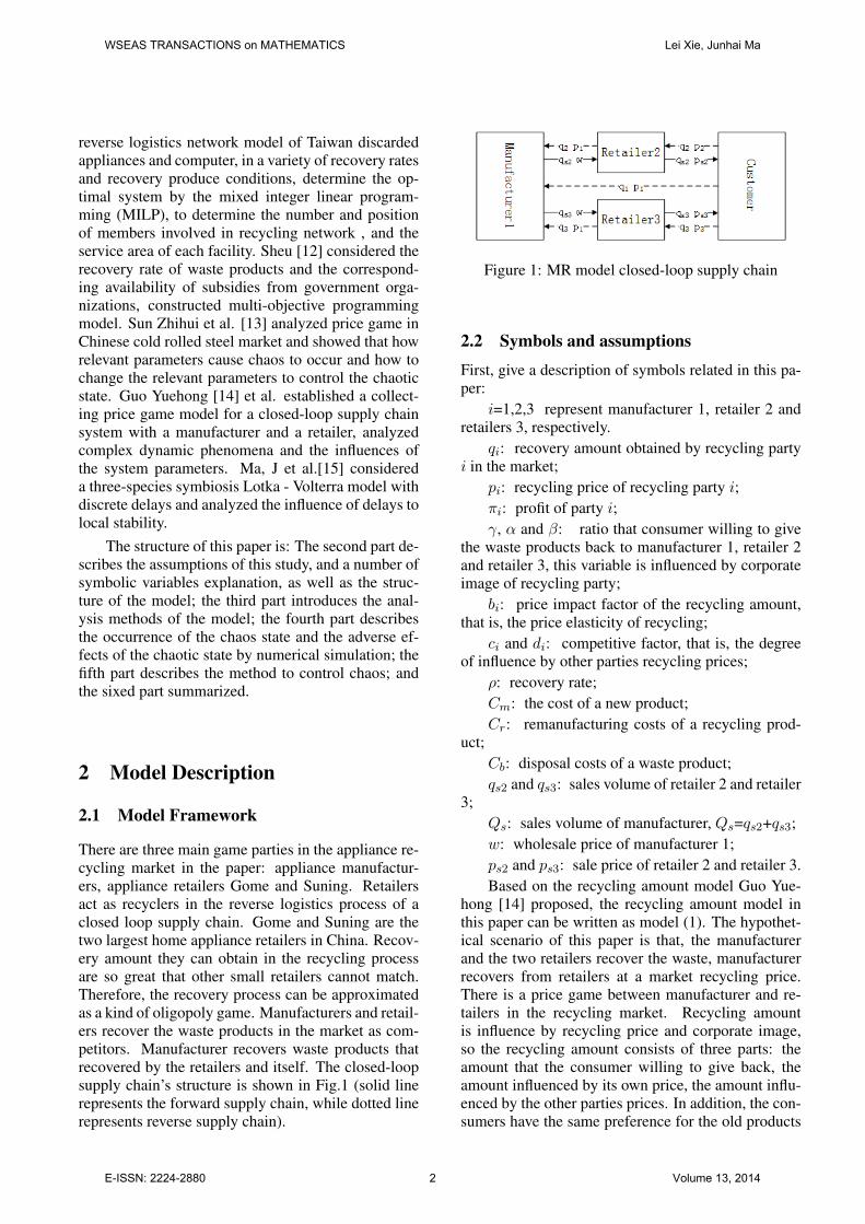
Through the above model, we can calculate theequilibrium price is p1 = 0.96, p2 = 0.50, p3 = 0.65.Based on the condition (10) and the above numericalsimulation, we can work out the stable region, it isshown as Fig.2.

When combination of g1, g2, g3 is in the stableregion, the system is in a steady state. It can alsobe observed through the evolution of the system asgi changes. Assuming g1 constant, when g1 and g2simultaneously changes, the evolution of the system


E-ISSN: 2224-2880 4 Volume 13, 2014

0.0

0.5

1.0

0.0

0.5

1.0

0.0

0.5

1.0

Figure 2: The stable region of the system

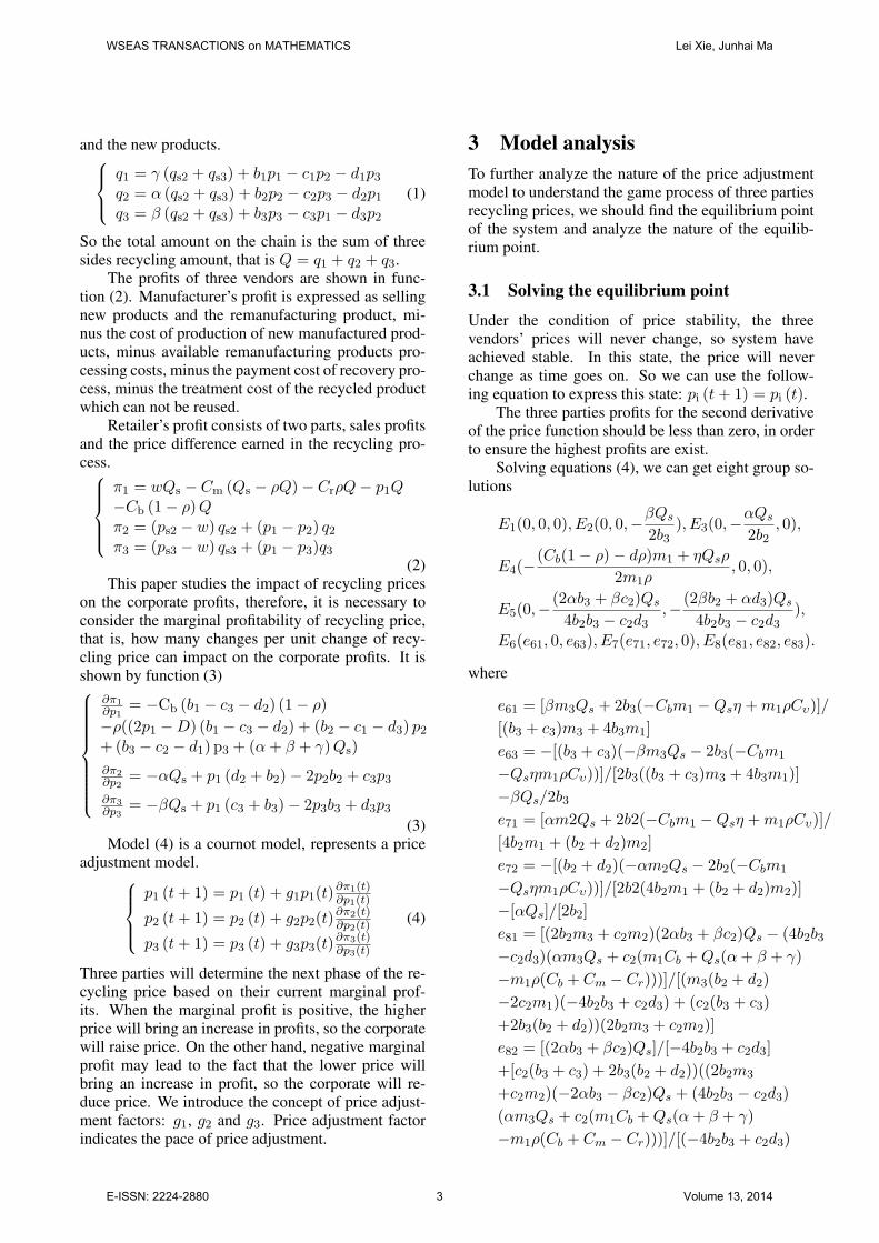
is shown as Fig.3. As can be seen, when gi is largerand larger, the system will enter into chaos state fromstable state. In order to analyze the impact of g3 tothe system expediently, we observe the impact of g3to the system by fixing g1 and g2. When g1 = 0.1,g2 = 0.1, we can observe how price adjustment fac-tor g3 of retailer 3 changes the three parties profitsand prices. According to the Routh-Hurwitz criterion,we can precisely calculate stability domain of g3 is0 <g3< 0.340.

00.1

0.20.3

0.40.5

0

0.2

0.4

0.6

0.80.9

0.95

1

1.05

1.1

1.15

p1

g3g2

Figure 3: Dynamic Evolution of P1 as g2, g2 changeswith g1=0.1

4.1 Lyapunov exponent and the dynamicevolution of the system

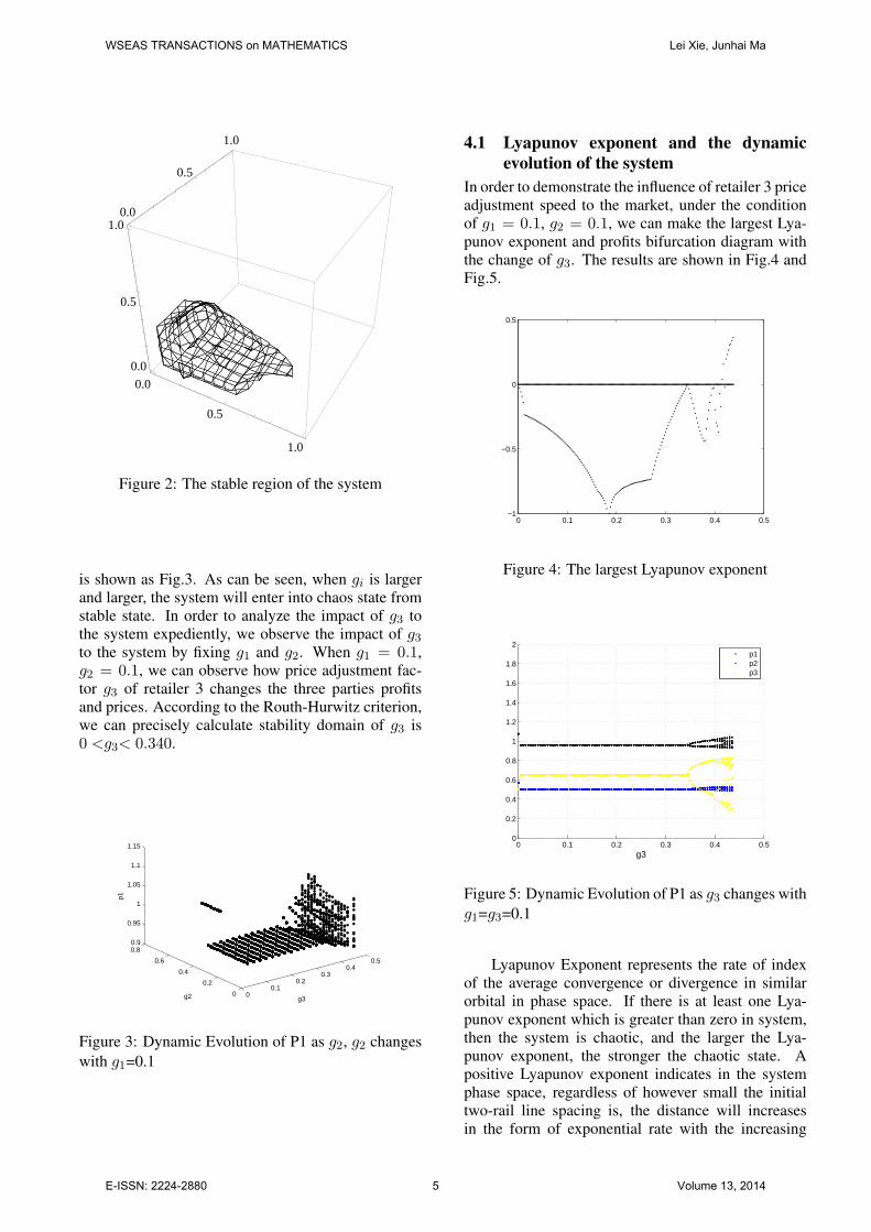
In order to demonstrate the influence of retailer 3 priceadjustment speed to the market, under the conditionof g1 = 0.1, g2 = 0.1, we can make the largest Lya-punov exponent and profits bifurcation diagram withthe change of g3. The results are shown in Fig.4 andFig.5.

0 0.1 0.2 0.3 0.4 0.5−1

−0.5

0

0.5

Figure 4: The largest Lyapunov exponent

0 0.1 0.2 0.3 0.4 0.50

0.2

0.4

0.6

0.8

1

1.2

1.4

1.6

1.8

2

g3

p1p2p3

Figure 5: Dynamic Evolution of P1 as g3 changes withg1=g3=0.1

Lyapunov Exponent represents the rate of indexof the average convergence or divergence in similarorbital in phase space. If there is at least one Lya-punov exponent which is greater than zero in system,then the system is chaotic, and the larger the Lya-punov exponent, the stronger the chaotic state. Apositive Lyapunov exponent indicates in the systemphase space, regardless of however small the initialtwo-rail line spacing is, the distance will increasesin the form of exponential rate with the increasing


E-ISSN: 2224-2880 5 Volume 13, 2014

of the number of iterations, and ultimately achievean unpredictable state, that is, chaos state. Fromlargest Lyapunov exponent, it can be seen that, in theinterval 0 <g3< 0.340, the maximum Lyapunov ex-ponent is less than zero, according to the definitionabove, its corresponding price is in a steady state,in the interval 0.34 < g3 < 0.40, the correspond-ing system is period-doubling bifurcation state, wheng3 = 0.40, the system reaches a second bifurcation,and so on. Until the largest Lyapunov exponent ofsystem is greater than 0 for the first time, from thispoint on, the system goes into chaos.

From system equilibrium dynamic evolutionchart of the recovery prices, it also easy to see thatwhen 0 < g3 < 0.340, the three parties equilibriumprice is stable. But when g3> 0.34, the recovery priceis beginning to go into the state of period-doublingbifurcation, until to the chaos. Meanwhile, usingMatlab software, we can easily calculate the systemtwo cycle bifurcation points are: (1.01,0.52,0.80),(0.95,0.50,0.44).

Similar as analysis of the equilibrium price, it canalso be observed that the influence of retailer 3 priceadjustment coefficient to three parties profits wheng1 = 0.1 and g2 = 0.1. The results are as shownin Fig.6 and Fig.7.

0 0.1 0.2 0.3 0.4 0.5150

155

160

165

170

175

180

g3

Pro

fit o

f M1

Figure 6: Dynamic Evolution of profit of manufac-turer as g3 changes with g1 = g2 = 0.1

It is obvious that, the bifurcation of the profit be-gins to appear when g3 = 0.34, the system goes into achaotic state. At this point, the market appears invalidvicious competition state.

4.2 Changes of recycling priceIn order to understand the recycle price changes overtime in the stability and chaos state, the following sim-ulates the changes in price. According to the above

0 0.1 0.2 0.3 0.4 0.522

22.5

23

23.5

24

24.5

25

25.5

26

g3

Pro

fit o

f Ret

aile

rs

Profit of R2Profit of R3

Figure 7: Dynamic Evolution of profit of retailers asg3 changes with g1=g2=0.1

analysis, it is easy to know the price adjustment factorg1 = 0.1, g2 = 0.1, g3 = 0.3 may represent a stablestate. At this point, the price of three vendors changeas shown in Fig.8.

0 20 40 60 80 1000

0.5

1

1.5

t

p

P1

P2

P3

Figure 8: Three vendors price changes when the sys-tem is in stable state

Similarly, when the system is in a chaotic statewith g1 = 0.1, g2 = 0.1, g3 = 0.43, the time series ofthree parties equilibrium price are as shown in Fig.9.It is obvious that when the system is in steady state,the three parties price will go into the stable state aftera brief recovery fluctuations; when the system is in achaotic state, the three parties price fluctuates all thetime, can not go into a stable state.

When the game runs after a certain period in astable system, it will get a set of stable equilibrium.When a sudden change occurs in one of the decision-making for some reason, it will break this equilibriumstate. But a stable system can make such mutation of


E-ISSN: 2224-2880 6 Volume 13, 2014

0 20 40 60 80 1000

0.5

1

1.5

t

p

P2P3

P1

Figure 9: Three vendors price changes when the sys-tem is in chaos state

decision variables gradually stabilized, so that the sys-tem can go back to its original equilibrium state. Asshown in Fig.10, when the game goes to the 20 cyclesand 60 cycles, changes in party decision variables willmake the system enter into a short unstable state, butwhen the game runs enough times, the system will bestable again.

0 20 40 60 80 100

−0.2

0

0.2

0.4

0.6

0.8

1

1.2

1.4

1.6

t

p

P1(61)=0.5

P1(21)=1.3

Figure 10: The influence of sudden changes in priceon the stability of system

4.3 Chaotic attractor and initial sensitivityg1 = 0.1, g2 = 0.1, g3 = 0.43 means a chaoticstate. In this chaotic state and initial recovery price ofp1=0.5, p2=0.5, p3=0.5, the system’s chaotic attractoris shown in Fig.11.

A distinctive feature of chaotic attractor is thatthe exponential segregation of attractor neighboringpoints, which indicates that chaotic systems have sen-sitive dependence on the initial conditions.

0

0.5

1

1.5

0

0.2

0.4

0.6

0.80

0.2

0.4

0.6

0.8

1

xy

z

Figure 11: The chaos attractor in a chaotic state withg1=0.1, g2=0.1, g3=0.43

The system in chaotic state has a certain sensitiv-ity to initial values, just as the butterfly effect, smallchanges in initial may bring enormous changes in ad-jacent tracks. In the chaotic state g1=0.1, g2 = 0.1,g3 = 0.43, the small changes in initial, from p1 = 0.5,p2 = 0.5, p3 = 0.5 to p1 = 0.5, p2 = 0.5,p3 = 0.5001, observe three parties recycling pricessensitivity to initial. Fig.12 and Fig.13 are analysis onthree recycling prices sensitivity to initial.

0 20 40 60 80 100−0.8

−0.6

−0.4

−0.2

0

0.2

0.4

0.6

t

p

Figure 12: The initial value sensitivity of three partiesrecycling prices with g1=0.1, g2=0.1, g3=0.43

It is obvious in Fig.12 that, in the case that theoriginal recovery price changes small, the differenceof three parties recycling prices is not obvious be-tween the two original prices conditions until t = 20.But as time goes on, the difference gradually emerged,and the maximum is more than 0.5. This differenceappears in retailer 3 whose price changes too fast.

On the other hand, the stable system is not af-


E-ISSN: 2224-2880 7 Volume 13, 2014

0 20 40 60 80 100−0.1

−0.05

0

0.05

0.1

0.15

t

p

Figure 13: The initial value sensitivity of three partiesrecycling prices with g1=0.1, g2=0.1, g3=0.3

fected by changes in the initial value. Fig.13 showsthat the price difference when the initial value changesfrom p1 = 0.5, p2 = 0.5, p3 = 0.5 to p1 = 0.5,p2 = 0.5, p3 = 0.6.

It is not difficult to see the stable system can playa role in stabilizing prices. But when the market isin a chaotic state, a small recycling price changesmay have a huge impact on the others’ recovery price.What is worse, the current price will have a huge im-pact on the next period recovery prices. In this case,the manufacturer is difficult to make accurate judg-ments on the market, and difficult to draw the best re-cycle price.

In summary, it is necessary to control the unstablestate.

5 Chaos controlIn a recovery market, the price equilibrium is short-term, temporary. The factors such as price adjustmentspeed, will broke equilibrium into the chaotic state.Once the market goes into the chaotic state, it willbe difficult for companies to adjust price to a suit-able state, to obtain a higher stable income. There-fore, a method of controlling chaos is needed. Thereare many ways of chaos control, such as the OGYmethod, continuous feedback control method, adap-tive control method, etc. In order to reflect the eco-nomic characteristics of the model, we use delayedfeedback control method, which belong to the contin-uous feedback control method.

The core idea of the delay control method is touse part of the information of the output signal feed-back to the system after a time delay, as an alterna-tive to an external input, and ultimately achieve sta-

bilization of unstable periodic orbits of chaotic attrac-tor. Response signal functions is the main differencebetween the delay control method and force feedbackcontrol method. Response signal function of delayedfeedback control method is:

f (t) = k [y (t− T )− y (t)] = kD(t) (11)

Function (11) is response signal function. Where,f(t) represents the control signal, k represents chaoscontrol factor, T is the delay time, in order to facili-tate the analysis of the economic characteristics of themodel, delay time the paper selected is 1. Thus thecontrol signal may be expressed by function (12):

f (t) = k [pi (t)− pi (t+ 1)] (12)

As this study is about the influence of retailer3 price adjustment factor to the chaotic phenomena,Therefore, we should exert control to retailer 3. Sosystem joined the chaos control signal can be ex-pressed as

p1 (t+ 1) = p1 (t) + g1p1 (t)∂π1(t)∂p1(t)

p2 (t+ 1) = p2 (t) + g2p2 (t)∂π2(t)∂p2(t)

p3 (t+ 1) = p3 (t) + g3p3 (t)∂π3(t)∂p3(t)

+ k[p3 (t)

−p3 (t+ 1)](13)

After adjustment, the model (13) can be writtenas

p1 (t+ 1) = p1 (t) + g1p1 (t)∂π1(t)∂p1(t)

p2 (t+ 1) = p2 (t) + g2p2 (t)∂π2(t)∂p2(t)

p3 (t+ 1) = p3 (t) +g31+kp3 (t)

∂π3(t)∂p3(t)

(14)

Also in chaotic state of g1=0.1, g2=0.1, g3=0.43,we consider the influence of chaos control factor k tothe system equilibrium prices.

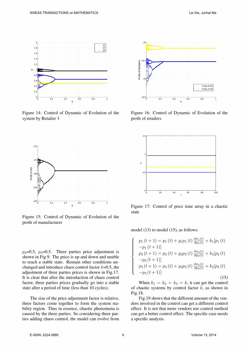
It is not difficult to see from the Fig.14, with thechaos control factor k increases, the system graduallygoes into the period-doubling bifurcation state from achaotic state, when k=0.26, the system begins to enterthe steady state. That is, when chaos control factork is greater than 0.26, the chaotic state is controlled.Similarly, we can change the state of chaos to observethe changes of k.

It is obvious that different chaotic state needs dif-ferent k to be controlled, with the retailer 3’s priceadjustment speed increases, the chaotic state needs agreater k to be controlled.

Similarity, we can also get the changes of 3 par-ties profits.

On condition that Price adjustment speed isg1=0.1, g2=0.1, g3=0.43 and Initial Price is p1=0.5,


E-ISSN: 2224-2880 8 Volume 13, 2014

0 0.2 0.4 0.6 0.8 10

0.2

0.4

0.6

0.8

1

1.2

1.4

1.6

1.8

2

k

p

p1p2p3

Figure 14: Control of Dynamic of Evolution of thesystem by Retailer 3

0 0.2 0.4 0.6 0.8 1155

160

165

170

175

k

Pro

fit o

f M1

Figure 15: Control of Dynamic of Evolution of theprofit of manufacturer

p2=0.5, p3=0.5. Three parties price adjustment isshown in Fig.9. The price is up and down and unableto reach a stable state. Remain other conditions un-changed and introduce chaos control factor k=0.5, theadjustment of three parties prices is shown in Fig.17.It is clear that after the introduction of chaos controlfactor, three parties prices gradually go into a stablestate after a period of time (less than 10 cycles).

The size of the price adjustment factor is relative,three factors come together to form the system sta-bility region. Thus in essence, chaotic phenomena iscaused by the three parties. So considering three par-ties adding chaos control, the model can evolve from

0 0.2 0.4 0.6 0.8 123.5

24

24.5

25

k

Pro

fit o

f Ret

aile

rs

Profit of R2Profit of R3

Figure 16: Control of Dynamic of Evolution of theprofit of retailers

0 20 40 60 80 1000

0.5

1

1.5

t

p

Figure 17: Control of price time array in a chaoticstate

model (13) to model (15), as follows:

p1 (t+ 1) = p1 (t) + g1p1 (t)∂π1(t)∂p1(t)

+ k1[p1 (t)

−p1 (t+ 1)]

p2 (t+ 1) = p2 (t) + g2p2 (t)∂π2(t)∂p2(t)

+ k2[p2 (t)

−p2 (t+ 1)]

p3 (t+ 1) = p3 (t) + g3p3 (t)∂π3(t)∂p3(t)

+ k3[p3 (t)

−p3 (t+ 1)](15)

When k1 = k2 = k3 = k, it can get the controlof chaotic systems by control factor k, as shown inFig.18.

Fig.19 shows that the different amount of the ven-dors involved in the control can get a different controleffect. It is not that more vendors use control methodcan get a better control effect. The specific case needsa specific analysis.


E-ISSN: 2224-2880 9 Volume 13, 2014

0 0.2 0.4 0.6 0.8 10

0.2

0.4

0.6

0.8

1

1.2

1.4

1.6

1.8

2

k

p

p1p2p3

Figure 18: Control of Dynamic of Evolution of thesystem by three vendors

0 0.2 0.4 0.6 0.8 10.9

0.92

0.94

0.96

0.98

1

1.02

1.04

1.06

1.08

1.1

k

p

Figure 19: The different control effect of the amountof vendors use control method

Based on function (11), we can change thecournot model (4) to function model (14). By replac-ing ∂π3

∂p3, we can get the function (16):

p3 (t+ 1) = p3 (t) +g31+kp3 (t) (−βQs + p1 (c3 + b3)

−2p3b3 + d3p2)(16)

In order to investigate the economic characteris-tics of the model, and use the economic argument toexplain the model, we transform chaos control func-tion (16) to function (17):

p3 (t+ 1) = p3 (t) + g3p3 (t) (− 2b31+kp3 +

c3+b31+k p1

+ d31+kp2 +

−β1+kQs)

(17)From function (16), we can easily to see, the de-

lay control method we used in this case can reducethe original price adjustment factor g3 to g3

1+k . It can

be seen as reducing the speed of the original price ad-justment. From function (17), we can see that in orderto avoid recycling prices going into chaotic state, sev-eral other parameters can be changed, in addition tocontrolling the price adjustment speed.

By means of integral, we can integrate the part ofthe function (17), and get the following formula (18):

(p1−p3)(b3

1 + kp3−

c31 + k

p1−d3

1 + kp2+

β

1 + kQs)

(18)Adding chaos control factor k is equal to making

the recycling amount function of retailer 3 become

q3 =β

1 + kQs+

b31 + k

p3−c3

1 + kp1−

d31 + k

p2 (19)

Chaos control factor k increases mean coefficientβ, b3, c3, d3 reduce respectively, and under the condi-tions of k > 0.26, Four coefficients will also have acertain degree of reduced.

It is obvious that it is an effective way to controlthe chaotic state by reducing the price elasticity, com-petitive factors, as well as the proportion of voluntary.That is, if one party price changes too fast, it shouldreduce voluntary recycling amount it can get, reducethe influence of its price to recovery amount, reducethe influence of the others price to recovery amount.

To achieve this purpose, the vendors should payattention to the recycling process and recycling ser-vices, in order to avoid consumers choosing the re-covery channel only by comparing recycling prices.In conclusion, the vendors should control their priceadjustment factors in a low degree. Or they shoulddo the following improvement to keep the system in astable state:

• To improve the quality of recycling service.

• To provide differentiated recovery services.

• To promote the importance of environmentalprotection to the consumers.

6 ConclusionThe paper analyzes recovery price of three parties inwaste household appliance market in China, proposesthat if price adjustments speed is too fast, the sys-tem will go into a chaotic state, and describes this ad-verse outcome of the chaotic state. Finally, we give achaos control method, and explain its economic sig-nificance.

To simplify the study, we consider only one man-ufacturer in the model, and we do not consider otherfactors such as government subsidies. Therefore, in


E-ISSN: 2224-2880 10 Volume 13, 2014

future studies, we can increase the number of manu-facturers, and introduce manufacturer game process inthe system. We can also add other factors to make themodel more perfect.

Acknowledgements: This work was supportedby National Natural Science Foundation of China61273231 and the Doctoral Scientific Fund Projectof the Ministry of Education of China (No.2013003211073).

References:

[1] A. D. Read, A weekly doorstep recycling collec-tion, I had no idea we could!: Overcoming thelocal barriers to participation. Resources, Con-servation and Recycling, Vol.26, 1999, pp.217-249.

[2] F. Melissen, Designing Collection Rate Enhanc-ing Measures for’small’Consumer Electronics,Technische Universiteit Eindhoven, 2003.

[3] C. Nagel, Take IT back-European approaches forsetting up logistics systems, Proceedings of the1998 IEEE International Symposium on, 1998.

[4] C. Nagel, and P. Meyer, Caught between ecologyand economy: end-of-life aspects of environ-mentally conscious manufacturing, Computers& industrial engineering, Vol.36, No.4, 1999,pp.781-792.

[5] H. R. Krikke, A. Van Harten, and P. C. Schuur,Business case Roteb: recovery strategies formonitors, Computers & Industrial Engineering,Vol.36, No.4, 1999, pp.739-757.

[6] Z. Istvan, and E. Garamvolgyi, Reverse logisticsand management of end-of-life electric products,2000, pp.15-19.

[7] A. Nagurney, and F. Toyasaki, Reverse supplychain management and electronic waste recy-cling:a multitiered network equilibrium frame-work for e-cycling, ransportation Research PartE: Logistics and Transportation Review, Vol.41,No.1 2005, pp.1-28.

[8] J. Lee, T. S. H, and M. Y. J, Present status ofthe recycling of waste electrical and electronicequipment in Korea, Resources, Conservationand Recycling, Vol.50, No.4, 2007, pp.380-397.

[9] M. Fleischmann, M. B. J, and R. Dekker,Quantitative models for reverse logistics: a re-view, European journal of operational research,Vol.103 No.1, 1997, pp.1-17.

[10] M. Fleischmann, P. Beullens, and M. B. R. J,The impact of product recovery on logistics net-work design, Production and operations man-agement, Vol.10 No.2, 2001, pp.156-173.

[11] H. S. Li, Reverse logistics system planning forrecycling electrical appliances and computers inTaiwan, Resources, conservation and recycling,Vol.32, No.1, 2001, pp.55-72.

[12] J. Sheu, and A. Y. Lin, Hierarchical facil-ity network planning model for global logisticsnetwork configurations, Applied MathematicalModelling, Vol.36, No.7, 2012, pp.3053-3066.

[13] Z. Sun, and J. Ma, Complexity of triopoly pricegame in Chinese cold rolled steel market, Non-linear Dynamics, Vol.67, No.3, 2012, pp.2001-2008.

[14] G. Yuehong, and M. Junhai, Research on gamemodel and complexity of retailer collecting andselling in closed-loop supply chain, AppliedMathematical Modelling, Vol.37 No.37, 2013,pp.5047-5058.

[15] J. Ma, Q. Zhang, and Q. Gao, Stability of a three-species symbiosis model with delays, NonlinearDynamics, Vol.67, No.1, 2012, pp.567-572.


E-ISSN: 2224-2880 11 Volume 13, 2014

the dangers of precipitous adjustment speed of recovery … · the dangers of precipitous...

Documents