The d-Level Nested Logit Model:Assortment and Price Optimization Problems

Guang Li Paat Rusmevichientong Huseyin Topaloglu

guangli@usc.edu rusmevic@marshall.usc.edu topaloglu@orie.cornell.edu

November 18, 2014 @ 4:04pm

Abstract

We consider assortment and price optimization problems under the d-level nested logit model. In the

assortment optimization problem, the goal is to find the revenue-maximizing assortment of products to offer,

when the prices of the products are fixed. Using a novel formulation of the d-level nested logit model as a

tree of depth d, we provide an efficient algorithm to find the optimal assortment. For a d-level nested logit

model with n products, the algorithm runs in O(dn log n) time. In the price optimization problem, the

goal is to find the revenue-maximizing prices for the products, when the assortment of offered products is

fixed. Although the expected revenue is not concave in the product prices, we develop an iterative algorithm

that generates a sequence of prices converging to a stationary point. Numerical experiments show that

our method converges faster than gradient-based methods, by many orders of magnitude. In addition to

providing solutions for the assortment and price optimization problems, we give support for the d-level

nested logit model by demonstrating that it is consistent with the random utility maximization principle

and equivalent to the elimination by aspects model.

1. Introduction

In their seminal work, Talluri and van Ryzin (2004) demonstrated the importance of incorporating

customer choice behavior when modeling demand in operations management problems. They

observed that customers make a choice among the available products after comparing them in

terms of price, quality, and possibly other features. This choice process creates interactions among

the demand for different products, and it is important to capture these interactions. One of the

models that is most commonly used to capture the choice process of customers among different

products is the multinomial logit model, pioneered by Luce (1959) and McFadden (1974). In this

paper, we consider the d-level nested logit model, allowing for an arbitrary number of levels d. In

this model, each product is described by a list of d features. As an example, if the products are

flight itineraries, then such features might include the departure time, fare class, airline, and the

number of connections. We describe the products by using a tree with d levels, where each level in

the tree corresponds to a particular feature. When choosing a product, a customer first chooses the

desired value of the first feature, say the departure time, which gives rise to a subset of compatible

1

flight itineraries. Then, she chooses the value of the second feature, which further narrows down

the set of compatible flight itineraries. Each subsequent feature selection reduces the compatible

set of flight itineraries further, until we are left with a single flight itinerary after d features have

been selected. In this way, each product corresponds to a leaf node in the tree, whose unique path

of length d from the root node describes the list of d features of the product.

We consider both assortment optimization and pricing problems under the d-level nested logit

model. In the assortment optimization problem, the prices of the product are fixed. The goal

is to find the revenue-maximizing assortment of products to offer. In the pricing problem, the

assortment of offered products is fixed, but the utility that a customer derives from a product

depends on the price of the product. The goal is to find the revenue-maximizing set of prices for

the products. We make contributions in terms of formulation of the d-level nested logit model,

solution to the assortment optimization problem and solution to the pricing problem. We proceed

to describing our contributions in each one of these three domains.

We provide a novel formulation of the d-level nested logit model using a tree of depth d. Building

on this formulation, we can describe the product selection probabilities through a succinct recursion

over the nodes of the tree. Using the succinct description of the product selection probabilities, we

formulate our assortment optimization and pricing problems. To our knowledge, this is the first

paper to present a description of the d-level nested logit model that works for an arbitrary tree

structure and an arbitrary number of levels.

We provide a complete solution to the assortment optimization problem. We give a recursive

characterization of the optimal assortment, which, in turn, leads to an efficient assortment

optimization algorithm for computing the optimal assortment. For a d-level nested logit model

with n products, the running time of the algorithm is O(dn log n). To our knowledge, this is the

first solution to the assortment optimization problem under the d-level nested logit model.

For the pricing problem, it is known that the expected revenue is not concave in the prices of

the products even when the customers choose according to the two-level nested logit model. Thus,

we cannot hope to find the optimal prices in general. Instead, we focus on finding stationary

points, corresponding to the prices at which the gradient of the expected revenue function is zero.

Using our recursive formulation of the d-level nested logit model, we give a simple expression for

the gradient of the expected revenue. Although our gradient expression allows us to compute a

stationary point by using a standard gradient ascent method, we find the gradient ascent method

to be relatively slow and it requires a careful selection of step size. We develop a new iterative

algorithm that generates a sequence of prices converging to a stationary point of the expected

2

revenue function. Our algorithm is different from gradient ascent because the prices it generates do

not follow the direction of the gradient. Furthermore, our algorithm completely avoids the problem

of choosing a step size. Numerical experiments show that our algorithm converges to a stationary

point of the expected revenue function much faster than gradient ascent.

2. Literature Review

We focus our literature review on papers that use variants of the multinomial and nested logit

models in assortment and price optimization problems. We refer the reader to Kok et al. (2006)

and Farias et al. (2013) for assortment optimization and pricing work under other choice models.

The multinomial logit model dates back to the work of Luce (1959) and it is known to be consistent

with random utility maximization. However, this model suffers from the independence of irrelevant

alternatives property, which implies that if a new product is added to an assortment, then the

demand for each existing product decreases by the same percentage. This property should not

hold when different products cannibalize each other to different extents and the multinomial logit

model can lead to biased estimates of the selection probabilities in such settings; see Train (2003).

The nested logit model avoids the independence of irrelevant alternatives property, while remaining

compatible with random utility maximization; see Borch-Supan (1990).

Talluri and van Ryzin (2004) and Gallego et al. (2004) consider assortment optimization

problems under the multinomial logit model. They show that the optimal assortment is revenue

ordered in the sense that it includes a certain number of products with the largest revenues. Liu

and van Ryzin (2008) provide an alternative proof of the same result. Gallego et al. (2011) consider

generalizations of the multinomial logit model, in which the attractiveness of the no purchase option

increases when more restricted assortments are offered to customers. They show that the assortment

problem under this choice model remains tractable and make generalizations to the network revenue

management setting, in which customers arriving into the system observe the assortment of available

fare classes and make a choice among them. Bront et al. (2009) and Rusmevichientong et al. (2013)

consider assortment optimization problems under the mixture of logits model. They show that

the problem is NP-hard, propose heuristic solution methods and investigate integer programming

formulations. The papers by van Ryzin and Mahajan (1999) and Li (2007) consider models in

which a firm needs to make joint assortment optimization and stocking quantity decisions. There

is a certain revenue and a procurement cost associated with each product. Once the firm chooses

the products to offer and their corresponding stocking quantities, a random number of customers

arrive into the system and each customer chooses among the offered products according to the

multinomial logit model. The goal is to choose the assortment of offered products and the stocking

3

quantities to maximize the expected profit. Li (2007) assumes that the demand for each product

is proportional to a random store traffic volume, whereas van Ryzin and Mahajan (1999) model

the demand for different products with random variables whose coefficients of variation decrease

with demand volume, capturing economies of scale. The paper by van Ryzin and Mahajan (1999)

assumes that products have the same profit margin and shows that the optimal assortment includes

a certain number of products with the largest attractiveness parameters in the choice model. If

there are p products, then their result reduces the number of assortments to consider to p. For a

nested logit model with m nests and p products in each nest, even if their ordering result holds in

each nest, the number of assortments to consider is pm.

Assortment optimization under the two-level nested logit model has been considered only

recently. Kok and Xu (2010) study joint assortment optimization and pricing problems under

the two-level nested logit model, where both the assortment of offered products and their prices are

decision variables. They work with two nest structures. In the first nest structure, customers first

choose a brand out of two brands, and then, a product type within the selected brand. In the second

nest structure, customers first choose a product category, and then, a brand for the selected product

category out of two brands. The authors show that the optimal assortment of product types within

each brand is popularity ordered, in the sense that it includes a certain number of product types

with the largest mean utilities. Thus, if there are p product types within each brand, then there

are p possible assortments of product types to consider in a particular brand. Since there are two

brands, the optimal assortment to offer is one of p2 assortments. The optimal assortment can be

found by checking the performance of all p2 assortments. The problem becomes intractable when

there is a large number of brands. If there are b brands, then the number of possible assortments to

consider is pb, which quickly gets large with b. We note that if we apply our assortment optimization

algorithm in Section 5 to the two-level nested logit model with b brands and p product types within

each brand, then the optimal assortment can be computed in O(2pb log(pb)) operations because

the total number of products is pb.

Davis et al. (2014) show how to compute the optimal assortment under the two-level nested logit

model with an arbitrary number of nests. Assuming that there are m nests and p products within

each nest (for a total of mp products), the authors show that there are only p possible assortments

of products to consider in each nest. Furthermore, they formulate a linear program to find the

best one of these assortment to choose from each nest. In this way, their approach avoids checking

the performance of all pm possible values for the optimal assortment. Gallego and Topaloglu

(2012) extend this work to accommodate a variety of constraints on the offered assortment. Li

and Rusmevichientong (2014) establish structural properties and use these properties to develop

4

a greedy algorithm for computing the optimal assortment. All work so far focuses on the two-

level nested logit model. To our knowledge, there is no assortment optimization work under the

general d-level nested logit model. The linear program proposed by Davis et al. (2014) and the

greedy algorithm developed by Li and Rusmevichientong (2014) do not generalize to the d-level

nested logit model. We note that, to our knowledge, assortment optimization problems under

other variants of logit models – the mixture of logits, the cross nested logits (Vovsha, 1997), paired

combinatorial and generalized nested logit models (Wen and Koppelman, 2001) – are not tractable.

In this paper, we show that the assortment optimization problem under the nested logit model is

tractable, regardless of the number of levels and the structure of the tree.

For pricing problems under the multinomial logit model, Hanson and Martin (1996) point out

that the expected revenue is not necessarily concave in prices. Song and Xue (2007) and Dong

et al. (2009) make progress by noting that the expected revenue is concave in market shares. Chen

and Hausman (2000) study the structural properties of the expected revenue function for a joint

product selection and pricing problem. There is some recent work on price optimization under the

two-level nested logit model. Li and Huh (2011) consider the case in which the products in the

same nest share the same price sensitivity parameter, and show that the expected revenue function

is concave in market shares. Gallego and Wang (2013) generalize this model to allow for arbitrary

price sensitivity parameters, but the expected revenue function is no longer concave in market

shares. Similar to assortment optimization, all of the earlier work on pricing under the nested logit

model focuses on two levels. Subsequent to our work, Li and Huh (2013) consider pricing problems

under the d-level nested logit model. They give a characterization of the optimal prices, but do not

provide an algorithm to compute them and do not address the assortment problem.

The rest of the paper is organized as follows. After the literature review in Section 2, we

describe the d-level nested logit model in Section 3 and formulate the assortment optimization

problem. In Section, 4, we give a characterization of the optimal assortment. This characterization

is translated into an algorithm for computing an optimal assortment in Section 5. In Section 6,

we test the numerical performance of our assortment optimization algorithm. In Section 7, we

formulate our pricing problem and give an algorithm to find a stationary point of the expected

revenue function. In Section 8, we give numerical experiments that test the performance of our

pricing algorithm. In Section 9, we provide practical motivation for the d-level nested logit model

by showing that it is compatible with random utility maximization principle and equivalent to the

elimination by aspects model. Also, we give practical situations where the assortment and price

optimization problems studied in this paper become useful. We conclude in Section 10.

5

3. Assortment Optimization Problem

We have n products indexed by {1, 2, . . . , n}, and the no-purchase option is denoted by

product 0. The taxonomy of the products is described by a d-level tree, denoted by T = (V,E)

with vertices V and edges E. The tree has n leaf nodes at depth d, corresponding to the n products

in {1, 2, . . . , n}. Throughout the paper, we will use the terms depth and level interchangeably. A

sample tree with d = 3 and n = 9 is given in Figure 1. The tree describes the process in which a

customer chooses a product. Starting at the root node, denoted by root, the edges emanating from

root represent the first criterion, or feature, that the customer uses in choosing her product. Each

node in the first level corresponds to subsets of products that fit with a particular value of the

first criterion. Product 0, corresponding to the no-purchase option, is labeled as node 0. It is

located in level one and directly connected to root, with no children. The edges in the second level

represent the second criterion that a customer uses to narrow down her choices, and each level-two

node represents a subset of products that are compatible with the particular values of the first two

criteria. The same interpretation applies to other levels. We use Children(j) to denote the set of

child nodes of node j in the tree, and Parent(j) to denote the parent node of node j.

Associated with each node j is a set of products Nj ⊆ {0, 1, . . . , n}, where Nj is the set of

products, or leaf nodes, that are included in the subtree rooted at node j. In particular, if j is a

leaf node, then Nj = {j}, which is just a singleton consisting of the product itself. On the other

hand, if j is a non-leaf node, then Nj =⋃· k∈Children(j)Nk, which is the disjoint union of the sets

of products at the child nodes of j. Note that if node j is in level h, then Nj corresponds to the

subset of products that fit with the specific values of the first h criteria, as specified by the path

from root to node j. We refer to a subset of products S ⊆ {1, 2, . . . , n} as an assortment. Each

assortment S defines a collection of subsets (Sj : j ∈ V) at each node of the tree with Sj ⊆ Nj ,

where if j is a leaf node other than node 0, then

Sj =

{j} if j ∈ S

∅ if j /∈ S .

If j corresponds to node 0, then we set S0 = {0} by convention. If j is a non-leaf node, then

Sj =⋃· k∈Children(j) Sk. Thus, Sj corresponds to the products in S that are included in the subtree

rooted at node j; that is, Sj = S ∩Nj . Often times, we refer to an assortment S by its collection of

subsets (Sj : j ∈ V), and write S = (Sj : j ∈ V). To illustrate the notation so far, we consider the

tree shown in Figure 1. Including the no-purchase option, there are 10 products in this tree, and they

are given by {0, 1, . . . , 9}. The nodes of the tree are indexed by {0, 1, . . . , 15}. We have, for example,

6

0 14 15

10 11 12 13

1 2 3 4 5 6 7 8 9

root

Figure 1: An illustration of the model formulation.

Children(10) = {1, 2, 3}, Parent(3) = 10, N2 = {2}, N10 = {1, 2, 3}, and N14 = {1, 2, 3, 4, 5}. For

an assortment S = {1, 3, 4, 6}, we have S1 = {1}, S2 = ∅, S10 = {1, 3}, S11 = {4}, S13 = ∅,

S14 = {1, 3, 4}, and Sroot = {0, 1, 3, 4, 6}.

Associated with each leaf node j, we have the attractiveness parameter vj , capturing the

attractiveness of the product corresponding to this leaf node. Given an assortment S = (Sj : j ∈ V),

a customer associates the preference weight Vj(Sj) with each node j ∈ V, which is a function

of the offered assortment S = (Sj : j ∈ V) and the attractiveness parameters of the products

(v1, . . . , vn). To make her choice, a customer starts from root in the tree and walks over the

nodes of the tree in a probabilistic fashion until she reaches a leaf node. In particular, if

the customer is at a non-leaf node j, then she follows node k ∈ Children(j) with probability

Vk(Sk)/∑

`∈Children(j) V`(S`). Thus, the customer is more likely to visit the nodes that have higher

preference weights. Once the customer reaches a leaf node, if this leaf node corresponds to a product,

then she purchases the product corresponding to this leaf node. If this leaf node corresponds to

the no-purchase option, then she leaves without making a purchase. As a function of the offered

assortment S = (Sj : j ∈ V) and the attractiveness parameters of the products (v1, . . . , vn), the

preference weight Vj(Sj) for each node j in the tree is computed as follows. If j is a leaf node, then

Sj is either {j} or ∅. In this case, the preference weight of a leaf node j is defined as Vj({j}) = vj

and Vj(∅) = 0. We assume that the no-purchase option, node 0, has a preference weight v0 so that

V0(S0) = v0. For each non-leaf node j, the preference weight of this node is computed as

Vj(Sj) =

∑k∈Children(j)

Vk(Sk)

ηj

, (1)

where ηj ∈ (0, 1] is a parameter of the nested logit model associated with node j. As we discuss

in Section 9, the d-level nested logit model can be derived by appealing to the random utility

maximization principle. Roughly speaking, 1− ηj is a measure of correlation between the utilities

7

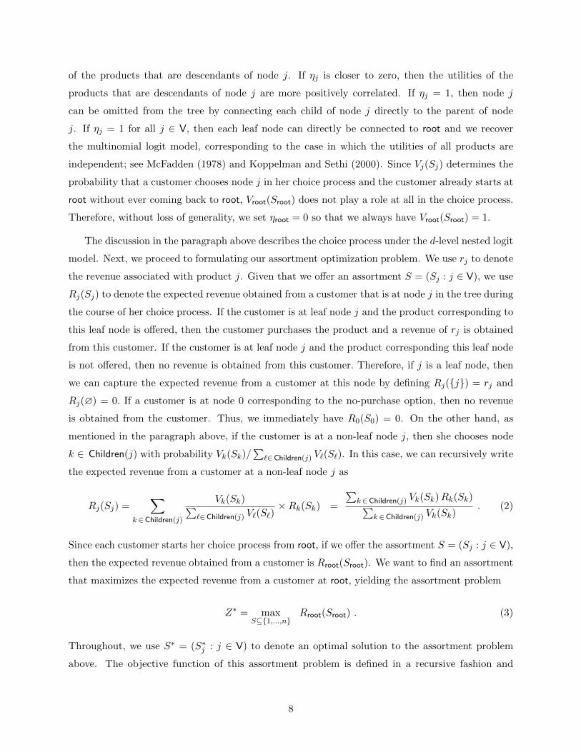
of the products that are descendants of node j. If ηj is closer to zero, then the utilities of the

products that are descendants of node j are more positively correlated. If ηj = 1, then node j

can be omitted from the tree by connecting each child of node j directly to the parent of node

j. If ηj = 1 for all j ∈ V, then each leaf node can directly be connected to root and we recover

the multinomial logit model, corresponding to the case in which the utilities of all products are

independent; see McFadden (1978) and Koppelman and Sethi (2000). Since Vj(Sj) determines the

probability that a customer chooses node j in her choice process and the customer already starts at

root without ever coming back to root, Vroot(Sroot) does not play a role at all in the choice process.

Therefore, without loss of generality, we set ηroot = 0 so that we always have Vroot(Sroot) = 1.

The discussion in the paragraph above describes the choice process under the d-level nested logit

model. Next, we proceed to formulating our assortment optimization problem. We use rj to denote

the revenue associated with product j. Given that we offer an assortment S = (Sj : j ∈ V), we use

Rj(Sj) to denote the expected revenue obtained from a customer that is at node j in the tree during

the course of her choice process. If the customer is at leaf node j and the product corresponding to

this leaf node is offered, then the customer purchases the product and a revenue of rj is obtained

from this customer. If the customer is at leaf node j and the product corresponding this leaf node

is not offered, then no revenue is obtained from this customer. Therefore, if j is a leaf node, then

we can capture the expected revenue from a customer at this node by defining Rj({j}) = rj and

Rj(∅) = 0. If a customer is at node 0 corresponding to the no-purchase option, then no revenue

is obtained from the customer. Thus, we immediately have R0(S0) = 0. On the other hand, as

mentioned in the paragraph above, if the customer is at a non-leaf node j, then she chooses node

k ∈ Children(j) with probability Vk(Sk)/∑

`∈Children(j) V`(S`). In this case, we can recursively write

the expected revenue from a customer at a non-leaf node j as

Rj(Sj) =∑

k∈Children(j)

Vk(Sk)∑`∈Children(j) V`(S`)

×Rk(Sk) =

∑k∈Children(j) Vk(Sk)Rk(Sk)∑

k∈Children(j) Vk(Sk). (2)

Since each customer starts her choice process from root, if we offer the assortment S = (Sj : j ∈ V),

then the expected revenue obtained from a customer is Rroot(Sroot). We want to find an assortment

that maximizes the expected revenue from a customer at root, yielding the assortment problem

Z∗ = maxS⊆{1,...,n}

Rroot(Sroot) . (3)

Throughout, we use S∗ = (S∗j : j ∈ V) to denote an optimal solution to the assortment problem

above. The objective function of this assortment problem is defined in a recursive fashion and

8

involves nonlinearities, but it turns out that we can solve this problem in a tractable manner.

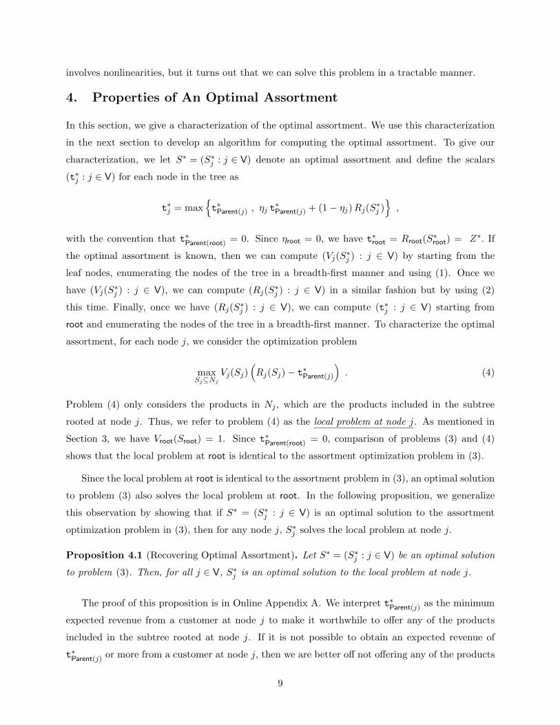
4. Properties of An Optimal Assortment

In this section, we give a characterization of the optimal assortment. We use this characterization

in the next section to develop an algorithm for computing the optimal assortment. To give our

characterization, we let S∗ = (S∗j : j ∈ V) denote an optimal assortment and define the scalars

(t∗j : j ∈ V) for each node in the tree as

t∗j = max{t∗Parent(j) , ηj t

∗Parent(j) + (1− ηj)Rj(S∗j )

},

with the convention that t∗Parent(root) = 0. Since ηroot = 0, we have t∗root = Rroot(S∗root) = Z∗. If

the optimal assortment is known, then we can compute (Vj(S∗j ) : j ∈ V) by starting from the

leaf nodes, enumerating the nodes of the tree in a breadth-first manner and using (1). Once we

have (Vj(S∗j ) : j ∈ V), we can compute (Rj(S

∗j ) : j ∈ V) in a similar fashion but by using (2)

this time. Finally, once we have (Rj(S∗j ) : j ∈ V), we can compute (t∗j : j ∈ V) starting from

root and enumerating the nodes of the tree in a breadth-first manner. To characterize the optimal

assortment, for each node j, we consider the optimization problem

maxSj⊆Nj

Vj(Sj)(Rj(Sj)− t∗Parent(j)

). (4)

Problem (4) only considers the products in Nj , which are the products included in the subtree

rooted at node j. Thus, we refer to problem (4) as the local problem at node j. As mentioned in

Section 3, we have Vroot(Sroot) = 1. Since t∗Parent(root) = 0, comparison of problems (3) and (4)

shows that the local problem at root is identical to the assortment optimization problem in (3).

Since the local problem at root is identical to the assortment problem in (3), an optimal solution

to problem (3) also solves the local problem at root. In the following proposition, we generalize

this observation by showing that if S∗ = (S∗j : j ∈ V) is an optimal solution to the assortment

optimization problem in (3), then for any node j, S∗j solves the local problem at node j.

Proposition 4.1 (Recovering Optimal Assortment). Let S∗ = (S∗j : j ∈ V) be an optimal solution

to problem (3). Then, for all j ∈ V, S∗j is an optimal solution to the local problem at node j.

The proof of this proposition is in Online Appendix A. We interpret t∗Parent(j) as the minimum

expected revenue from a customer at node j to make it worthwhile to offer any of the products

included in the subtree rooted at node j. If it is not possible to obtain an expected revenue of

t∗Parent(j) or more from a customer at node j, then we are better off not offering any of the products

9

included in the subtree rooted at node j. To see this interpretation, note that if S∗ = (S∗j : j ∈ V)

is an optimal assortment for problem (3), then by Proposition 4.1, S∗j solves the local problem at

node j. Also, the optimal objective value of the local problem at node j has to be non-negative,

because the empty set trivially yields an objective value of zero for problem (4). Thus, if S∗j 6= ∅

so that it is worthwhile to offer any of the products included in the subtree rooted at node j, then

we must have Rj(S∗j ) ≥ t∗Parent(j). Otherwise, S∗j provides a negative objective value for the local

problem at node j, contradicting the fact that S∗j solves the local problem at node j.

If j is a leaf node, then the local problem at node j given in (4) can be solved efficiently because

Nj = {j} so that Sj is simply either {j} or ∅. The crucial question is whether we can use a

bottom-up approach and construct a solution for the local problem at any node j by using the

solutions to the local problems at its child nodes. The following theorem affirmatively answers this

question by showing that we can synthesize the solution of the local problem at node j by using

the solutions of the local problems at each of its children.

Theorem 4.2 (Synthesis from Child Nodes). Consider an arbitrary non-leaf node j ∈ V. If for all

k ∈ Children(j), Sk is an optimal solution to the local problem at node k, then⋃· k∈Children(j) Sk is

an optimal solution to the local problem at node j.

Thus, if we solve the local problem at all nodes k ∈ Children(j) and take the union of the optimal

solutions, then we obtain an optimal solution to the local problem at node j. We give the proof of

Theorem 4.2 in Online Appendix A. In Section 5, we use this theorem to develop an algorithm for

computing the optimal assortment. The next corollary shows that the optimal assortment can be

obtained by comparing the revenues of the products with the scalars (t∗j : j ∈ V).

Corollary 4.3 (Revenue Comparison). Let S ={` ∈ {1, 2, . . . , n} : r` ≥ t∗Parent(`)

}. Then, S is an

optimal solution to problem (3).

Proof: Let Sj ≡ S ∩Nj ={` ∈ Nj : r` ≥ t∗Parent(`)

}, in which case, Sroot = S. By induction on the

depth of node j, we will show that Sj is an optimal solution to the local problem at node j. Since

the local problem at root is identical to problem (3), the desired result follows. If j is a leaf node,

then Nj = {j}, Rj({j}) = rj , Vj({j}) = vj , and Rj(∅) = Vj(∅) = 0. So,

arg maxSj⊆Nj

Vj(Sj)(Rj(Sj)− t∗Parent(j)

)= arg max

{vj

(rj − t∗Parent(j)

), 0}

=

{j} if rj ≥ t∗Parent(j)

∅ if rj < t∗Parent(j)

= Sj ,

10

establishing the result for a leaf node j. Now, suppose that the result is true for all nodes at depth

h and consider node j at depth h − 1. By the induction hypothesis, for all k ∈ Children(j), Sk

is an optimal solution to the local problem at node k. So, by Theorem 4.2,⋃· k∈Children(j) Sk is an

optimal solution to the local problem at node j. To complete the proof, note that

⋃·

k∈Children(j)

Sk =⋃·

k∈Children(j)

{` ∈ Nk : r` ≥ t∗Parent(`)

}={` ∈ Nj : r` ≥ t∗Parent(`)

}= Sj ,

where the second equality uses the fact that Nj =⋃· k∈Children(j)Nk. 2

By the above result, if product ` is in the optimal assortment, then any larger-revenue product

sharing the same parent with product ` is also in the optimal assortment. As shown below, for a

tree with one or two levels, this result recovers the optimality of revenue ordered assortments found

in the existing literature for the multinomial and two-level nested logit models.

Example 4.4 (Multinomial Logit). The multinomial logit model with n products, indexed by

{1, 2, . . . , n}, corresponds to a one-level nested logit model, with n + 1 leaf nodes connected to

root. The first n of these nodes correspond to individual products and the last one corresponds

to the no-purchase option. Since these is only one level in the tree, each leaf node has root as its

parent. So, it follows from Corollary 4.3 that an optimal assortment is given by

S∗ ={` ∈ {1, 2, . . . , n} : r` ≥ t∗Parent(`)

}= {` ∈ {1, 2, . . . , n} : r` ≥ Z∗} ,

where the second equality follows because t∗Parent(`) = t∗root = Z∗. The last expression above shows

that if a particular product is in the optimal assortment, then any product with a larger revenue

is in the optimal assortment as well.

Example 4.5 (Two-Level Nested Logit). In the two-level nested logit model, the set of n products

{1, 2, . . . , n} =⋃· mi=1Ni is a disjoint union of m sets. The products in Ni are said to be in nest i. In

this case, the associated tree has m + 1 first-level nodes. The last one of these first-level nodes

corresponds to the no-purchase option. For the other m first-level nodes, each first-level node i has

|Ni| children. Using Corollary 4.3, we have

S∗ ={` ∈ {1, . . . , n} : r` ≥ t∗Parent(`)

}=

m⋃·i=1

{` ∈ Ni : r` ≥ t∗Parent(`)

}=

m⋃·i=1

{` ∈ Ni : r` ≥ t∗i

},

where the last equality uses the fact that the node corresponding to each product ` in nest i has

the first-level node i as its parent. The last expression above shows that if a product in nest i is

included in the optimal assortment, then any product in this nest with a larger revenue is included

11

in the optimal assortment as well. This characterization of the optimal assortment for the two-level

nested logit model was proved in Davis et al. (2014).

5. An Algorithm for Assortment Optimization

In this section, we use the characterization of an optimal assortment given in Section 4 to develop

an algorithm that can be used to solve the assortment optimization problem in (3). For any set X,

let 2X denote the collection of all subsets of X. To find an optimal assortment, for each node j,

we will construct a collection of subsets Aj ⊆ 2Nj such that Aj includes an optimal solution to the

local problem at node j. As pointed out in Section 4, the local problem at root is identical to the

assortment optimization problem in (3). Thus, the collection Aroot includes an optimal solution to

problem (3) and if the collection Aroot is reasonably small, then we can check the expected revenue

of each subset in Aroot to find the optimal assortment.

To construct the collection Aj for each node j, we start from the leaf nodes and move up the

tree by going over the nodes in a breadth-first manner. If ` is a leaf node, then N` = {`}, so that

the optimal solution to the local problem at node ` is either {`} or ∅. Thus, if we let A` = {{`},∅}

for each leaf node `, then the collection A` includes an optimal solution to the local problem at

node `. Now, consider a non-leaf node j and assume that for each node k ∈ Children(j), we

already have a collection Ak that includes an optimal solution to the local problem at node k. To

construct a collection Aj that includes an optimal solution to the local problem at node j, for each

k ∈ Children(j) and u ∈ R, we let Sk(u) be an optimal solution to the problem

maxSk∈Ak

Vk(Sk) (Rk(Sk)− u) . (5)

Note that problem (5) considers only the subsets in the collection Ak. We claim that the collection{⋃· k∈Children(j) Sk(u) : u ∈ R

}includes an optimal solution to the local problem at node j.

Claim 1: Let Aj ={⋃· k∈Children(j) Sk(u) : u ∈ R

}. Then, the collection of subsets Aj includes an

optimal solution to the local problem at node j given in problem (4).

The objective function of problem (5) with u = t∗Parent(k) is identical to the objective function of

the local problem at node k. Furthermore, by our hypothesis, Ak includes an optimal solution to the

local problem at node k. Thus, if we solve problem (5) with u = t∗Parent(k), then the optimal solution

Sk(t∗Parent(k)) is an optimal solution to the local problem at node k. In this case, Theorem 4.2 implies

that the assortment⋃· k∈Children(j) Sk(t

∗Parent(k)) is an optimal solution to the local problem at node

j. Since⋃· k∈Children(j) Sk(t

∗Parent(k)) ∈ Aj , the collection Aj includes an optimal solution to the local

problem at node j, establishing the claim.

12

�

��,���(�)

��,���(�)

��,���(�)

��,�� (�)

��� ��

� ���

Figure 2: The lines {Lk,Sk(·) : Sk ∈ Ak} and the points {Iqk : q = 0, . . . , Qk} for some collection

Ak = {S1k , S

2k , S

3k , S

4k}.

Next, we show that all of the subsets in the collection Aj ={⋃· k∈Children(j) Sk(u) : u ∈ R

}can

be constructed in a tractable fashion.

Claim 2: We have |Aj | ≤∑

k∈Children(j) |Ak|, and all of the subsets in the collection Aj can be

computed in O(∑

k∈Children(j) |Ak| log |Ak|)

operations.

For each Sk ∈ Ak, let Lk,Sk(u) = Vk(Sk) (Rk(Sk) − u), in which case, problem (5) can be

written as maxSk∈Ak Lk,Sk(u). Since Lk,Sk(u) is a linear function of u, with slope −Vk(Sk) and

y-intercept Vk(Sk)Rk(Sk), problem (5) reduces to finding the highest line at point u among the lines

{Lk,Sk(·) : Sk ∈ Ak}. By checking the pairwise intersection points of the lines {Lk,Sk(·) : Sk ∈ Ak},

we can find points −∞ = I0k ≤ I1

k ≤ . . . ≤ IQk−1k ≤ IQkk = ∞ with Qk = |Ak| such that the

highest one of the lines {Lk,Sk(·) : Sk ∈ Ak} does not change as long as u takes values in one of the

intervals {[Iq−1k , Iqk ] : q = 1, . . . , Qk}. Figure 2 shows an example of the lines {Lk,Sk(·) : Sk ∈ Ak}

for some collection Ak = {S1k , S

2k , S

3k , S

4k}. The solid lines in this figure correspond to the lines in

{Lk,Sk(·) : Sk ∈ Ak} and the circles correspond to the points in {Iqk : q = 0, . . . , Qk}, with Qk = 4,

I0k = −∞ and I4

k = ∞. Thus, the discussion in this paragraph shows that we can construct Qk

intervals {[Iq−1k , Iqk ] : q = 1, . . . , Qk} such that these intervals partition the real line and the optimal

solution to problem (5) does not change when u takes values in one of these intervals. It is a standard

result in analysis of algorithms that we can compute the intersection points {Iqk : q = 0, . . . , Qk}

using O(Qk logQk) = O(|Ak| log |Ak|) operations; see Kleinberg and Tardos (2005).

Following the approach described in the above paragraph, we can construct the collection of

points {Iqk : q = 0, . . . , Qk} for all k ∈ Children(j). Putting these collections together, we obtain the

13

collection of points⋃· k∈Children(j){I

qk : q = 0, . . . , Qk}. Note that I0

k = −∞ and IQkk = ∞ for all

k ∈ Children(j). Ordering the points in this collection in increasing order and removing duplicates

at −∞ and ∞, we obtain the collection of points {Iqj : q = 0, . . . , Qj}, with −∞ = I0j ≤ I1

j ≤ . . . ≤

IQj−1j ≤ I

Qjj = ∞. Note that Qj ≤ 1 +

∑k∈Children(j)(Qk − 1) ≤

∑k∈Children(j)Qk. The points

{Iqj : q = 0, . . . , Qj} will form the basis for constructing the collection of subsets Aj .

We make a crucial observation. Consider an arbitrary interval [Iq−1j , Iqj ], with 1 ≤ q ≤ Qj . By

our construction of the points {Iqj : q = 0, . . . , Qj} in the above paragraph, for all k ∈ Children(j),

there exists some index 1 ≤ ζk ≤ Qk such that [Iq−1j , Iqj ] ⊆ [Iζk−1

k , Iζkk ]. On the other hand,

we recall that the optimal solution to problem (5) does not change as u takes values in one of

the intervals {[Iq−1k , Iqk ] : q = 1, . . . , Qk}. Therefore, since [Iq−1

j , Iqj ] ⊆ [Iζk−1k , Iζkk ], the optimal

solution to problem (5) does not change when u takes values in the interval [Iq−1j , Iqj ]. In other

words, the collection of subsets{Sk(u) : u ∈ [Iq−1

j , Iqj ]}

can be represented by just a single subset ,

which implies that the collection of subsets{⋃· k∈Children(j) Sk(u) : u ∈ [Iq−1

j , Iqj ]}

can also be

represented by a single subset. Let Sqj denote the single subset that represents the collection

of subsets{⋃· k∈Children(j) Sk(u) : u ∈ [Iq−1

j , Iqj ]}

. In this case, we obtain

Aj ={⋃· k∈Children(j) Sk(u) : u ∈ R

}=

Qj⋃·

q=1

{⋃· k∈Children(j) Sk(u) : u ∈ [Iq−1

j , Iqj ]}

={Sqj : q = 1, 2, . . . , Qj

}. (6)

Thus, the number of subsets in the collection Aj satisfies |Aj | = Qj ≤∑

k∈Children(j)Qk =∑k∈Children(j) |Ak|. Finally, the number of operations required to compute the collection Aj is

equal to the running time for computing the intersection points {Iqk : q = 0, . . . , Qk} for each

k ∈ Children(j), giving the total running time of O(∑

k∈Children(j) |Ak| log |Ak|)

. The following

lemma summarizes the key findings from the above discussion.

Lemma 5.1. Consider an arbitrary non-leaf node j ∈ V. For each k ∈ Children(j), suppose there

exists a collection of subsets Ak ⊆ 2Nk such that Ak contains an optimal solution to the local

problem at node k. Then, we can construct a collection of subsets Aj ⊆ 2Nj such that Aj includes

an optimal solution to the local problem at node j with |Aj | ≤∑

k∈Children(j) |Ak|. Moreover, this

construction requires O(∑

k∈Children(j) |Ak| log |Ak|)

operations.

To obtain an optimal assortment, we iteratively apply Lemma 5.1 starting at the leaf nodes. For

each leaf node `, letting A` = {{`},∅} suffices. Then, using the above construction and going over

the nodes in a breadth-first manner, we can construct the collection Aj for every node j in the

tree. To find an optimal assortment, we check the expected revenue of each subset in the collection

14

3

0 14 15

10 11 12 13

1 2 4 5 6 7 8 9

root

j 0 1 2 3 4 5 6 7 8 9 10 11 12 13 14 15 root

vj 17 4 5 10 6 9 4 7 10 13 · · · · · · ·rj 0 14.8 9 5 13.4 7.5 15 8 18 6 · · · · · · ·ηj · · · · · · · · · · 0.93 0.87 0.89 0.67 0.75 0.9 0

Figure 3: A three-level problem instance and its parameters.

Aroot and choose the subset that provides the largest expected revenue. The following theorem

shows that all of this work can be done in O(dnlog n) operations.

Theorem 5.2. For each node j ∈ V, we can construct a collection Aj ⊆ 2Nj such that |Aj | ≤ 2n

and Aj includes an optimal solution to the local problem at node j. Moreover, constructing Aj for

all j ∈ V requires O(dnlog n) operations.

As a function of {|Ak| : k ∈ Children(j)}, Lemma 5.1 bounds the number of subsets in the

collection Aj and gives the number of operations required to construct the collection Aj . We can

show Theorem 5.2 by using these relationships iteratively. The details are in Online Appendix B.

6. Numerical Illustrations for Assortment Optimization

In this section, we demonstrate our assortment optimization algorithm on one small problem

instance and report its practical performance when applied on large problem instances. For the

demonstration purpose, we consider a three-level nested logit model with nine products indexed by

1, 2, . . . , 9, along with a no-purchase option. We index the nodes of the tree by {0, 1, . . . , 15}∪{root},

where the nodes {0, 1, . . . , 9} correspond to leaf nodes and the rest are non-leaf nodes. The top

portion of Figure 3 shows the organization of the tree, whereas the bottom portion shows the model

parameters. The parameters rj and vj are given for each leaf node j, whereas the parameter ηj is

given for each non-leaf node j.

For this problem instance, if we let A10 = {{1, 2, 3}, {1, 2}, {1},∅}, then one can verify that

this collection includes an optimal solution to the local problem at node 10. Similarly, if we let

A11 = {{4, 5}, {4},∅}, then this collection includes an optimal solution to the local problem at node

11. By using the discussion in Section 5, we will construct a collection A14 such that this collection

15

S10 {1, 2, 3} {1, 2} {1} ∅V10(S10) 15.46 7.72 3.63 0

V10(S10)R10(S10) 125.48 89.35 53.73 0

Optimal in Interval [−∞, 4.67] [4.67, 8.72] [8.72, 14.80] [14.80,∞]

S11 {4, 5} {4} ∅V11(S11) 10.55 4.75 0

V11(S11)R11(S11) 104.01 63.69 0

Optimal in Interval [−∞, 6.96] [6.96, 13.40] [13.40,∞]

u [−∞, 4.67] [4.67, 6.96] [6.96, 8.72] [8.72, 13.40] [13.40, 14.80] [14.8,∞]

S10(u) ∪· S11(u) {1, 2, 3, 4, 5} {1, 2, 4, 5} {1, 2, 4} {1, 4} {1} ∅

Table 1: Computation of A14. The top two portions show the solution to problem (5) for k = 10and k = 11, respectively, for every value of u ∈ R. The bottom portion lists each subset in A14.

includes an optimal solution to the local problem at node 14. To that end, for each S10 ∈ A10,

we consider the line L10,S10(u) = V10(S10) (R10(S10)− u) with the slope −V10(S10) and y-intercept

V10(S10) × R10(S10). The second and third rows in the top portion of Table 1 list the slopes

and intercepts for the lines corresponding to the four assortments in the collection A10. Finding

the pairwise intersection points of these four lines, we determine that if u ∈ [−∞, 4.67], then the

highest one of these lines is the one corresponding to the subset {1, 2, 3}. Similarly, if u ∈ [4.67, 8.72],

then the highest line is the one corresponding to the subset {1, 2}. In other words, following the

notation in Section 5, if u ∈ [−∞, 4.67], then the optimal solution to problem (5) for k = 10

is given by S10(u) = {1, 2, 3}. Similarly, if u ∈ [4.67, 8.72], then S10(u) = {1, 2}. The last row

in the top portion of Table 1 lists the intervals such that if u belongs to one of these intervals,

then S10(u) takes the value in the first row. Thus, the points {Iq10 : q = 0, 1, . . . , 4} are given by

{−∞, 4.67, 8.72, 14.80,∞}. The middle portion of Table 1 focuses on the lines corresponding to

the assortments in the collection A11. The formats of the top and middle portions of the table

are the same. Thus, the points {Iq11 : q = 0, 1, . . . , 3} are given by {−∞, 6.96, 13.40,∞}. Taking

the union of these two sets of points, we obtain {−∞, 4.67, 6.96, 8.72, 13.40, 14.80,∞}. In this

case, we note that if u ∈ [−∞, 4.67], then the optimal solution to problem (5) for k = 10 is

given by S10(u) = {1, 2, 3}, whereas the optimal solution to problem (5) for k = 11 is given by

S11(u) = {4, 5}. Thus, if u ∈ [−∞, 4.67], then⋃· k∈Children(14) Sk(u) = {1, 2, 3, 4, 5}. Similarly, if

u ∈ [4.67, 6.96], then the optimal solution to problem (5) for k = 10 is given by S10(u) = {1, 2},

whereas the optimal solution to problem (5) for k = 11 is given by S11(u) = {4, 5}, which implies

that if u ∈ [4.67, 6.96], then⋃· k∈Children(14) Sk(u) = {1, 2, 4, 5}. Following this line of reasoning, the

bottom portion of Table 1 lists⋃· k∈Children(14) Sk(u) for every value of u ∈ R. Noting (6), we have

A14 ={⋃· k∈Children(14) Sk(u) : u ∈ R

}= {{1, 2, 3, 4, 5}, {1, 2, 4, 5}, {1, 2, 4}, {1, 4}, {1},∅}.

16

S12 {6, 7} {6} ∅V12(S12) 8.45 3.43 0

V12(S12)R12(S12) 89.11 51.51 0Optimal in Interval [−∞, 7.50] [7.50, 15.00] [15.00,∞]

S13 {8, 9} {8} ∅V13(S13) 8.17 4.68 0

V13(S13)R13(S13) 91.67 84.19 0Optimal in Interval [−∞, 2.14] [2.14, 18.00] [18.00,∞]

u [−∞, 2.14] [2.14, 7.50] [7.50, 15.00] [15.00, 18.00] [18.00,∞]

S12(u) ∪· S13(u) {6, 7, 8, 9} {6, 7, 8} {6, 8} {8} ∅

Table 2: Computation of A15. The top two portions show the solution to problem (5) for k = 12and k = 13, respectively, for every value of u ∈ R. The bottom portion lists each subset in A15.

On the other hand, if we let A12 = {{6, 7}, {6},∅}, then one can verify that this collection

includes an optimal solution to the local problem at node 12. Similarly, if we let A13 =

{{8, 9}, {8},∅}, then this collection includes an optimal solution to the local problem at node

13. We use an argument similar to the one in the above paragraph to construct a collection A15

from the collections A12 and A13, such that the collection A15 includes an optimal solution to the

local problem at node 15. Table 2 gives the details of our computations. The format of this table

is identical to that of Table 1. The last row of the top portion shows that when u takes values

in the intervals [−∞, 7.50], [7.50, 15.00] and [15.00,∞], the optimal solution to problem (5) for

k = 12 is, respectively, S12(u) = {6, 7}, S12(u) = {6} and S12(u) = ∅. The last row of the middle

portion shows that when u takes values in the intervals [−∞, 2.14], [2.14, 18.00] and [18.00,∞],

the optimal solution to problem (5) for k = 13 is, respectively, S13(u) = {8, 9}, S13(u) = {8} and

S13(u) = ∅. Collecting these results together, the last row of the bottom portion of Table 2, under

the heading S12(u) ∪· S13(u), lists⋃· k∈Children(15) Sk(u) for every value of u ∈ R. Thus, we have

A15 = {{6, 7, 8, 9}, {6, 7, 8}, {6, 8}, {8},∅}.

We have the collections A14 and A15 such that these collections include an optimal solution to

the local problems at nodes 14 and 15, respectively. Finally, we use these collections to construct

a collection Aroot such that this collection includes an optimal solution to the local problem at

root. Our computations are given in Table 3 and they are similar to those in Tables 1 and 2. For

example, the last row of the top portion shows that when u takes values in the intervals [−∞, 3.02]

and [3.02, 5.50], the optimal solution to problem (5) for k = 14 is, respectively, S14(u) = {1, 2, 3, 4, 5}

and S14(u) = {1, 2, 4, 5}. The last row of the middle portion shows that when u takes values in the

intervals [−∞, 1.05] and [1.05, 6.69], the optimal solution to problem (5) for k = 15 is, respectively,

S15(u) = {6, 7, 8, 9} and S15(u) = {6, 7, 8}. Collecting these results together, the second row of the

bottom portion of Table 3, under the heading S14(u) ∪· S15(u), lists⋃· k∈Children(root) Sk(u) for every

17

S14 {1, 2, 3, 4, 5} {1, 2, 4, 5} {1, 2, 4} {1, 4} {1} ∅V14(S14) 11.52 8.84 6.64 4.93 2.63 0

V14(S14)R14(S14) 101.62 93.53 81.44 69.01 38.92 0Highest in Interval [−∞, 3.02] [3.02, 5.50] [5.50, 7.27] [7.27, 13.10] [13.10, 14.80] [14.80,∞]

S15 {6, 7, 8, 9} {6, 7, 8} {6, 8} {8} ∅V15(S15) 12.55 10.15 6.58 4.01 0

V15(S15)R15(S15) 136.48 133.96 110.08 72.16 0Highest in Interval [−∞, 1.05] [1.05, 6.69] [6.69, 14.75] [14.75, 18.00] [18.00,∞]

u [−∞, 1.05] [1.05, 3.02] [3.02, 5.50] [5.50, 6.69] [6.69, 7.27]

S14(u) ∪· S15(u) {1, 2, 3, 4, 5, 6, 7, 8, 9} {1, 2, 3, 4, 5, 6, 7, 8} {1, 2, 4, 5, 6, 7, 8} {1, 2, 4, 6, 7, 8} {1, 2, 4, 6, 8}Rroot(S14(u) ∪· S15(u)) 5.80 6.09 6.32 6.38 6.34

u [7.27, 13.10] [13.10, 14.75] [14.75, 14.80] [14.80, 18.00] [18.00,∞]

S14(u) ∪· S15(u) {1, 4, 6, 8} {1, 6, 8} {1, 8} {8} ∅Rroot(S14(u) ∪· S15(u)) 6.28 5.68 4.70 3.43 0.00

Table 3: Computation of Aroot. The top two portions show the solution to problem (5) for k = 14and k = 15, respectively, for every value of u ∈ R. The bottom portion lists each subset in Aroot.

value of u ∈ R. These subsets form the collection Aroot, which includes an optimal solution to the

local problem at root. Since the local problem at root is equivalent to our assortment optimization

problem, the collection Aroot includes an optimal assortment. The last row of the bottom portion of

Table 3, under the heading Rroot(S14(u)∪· S(u)15), lists the expected revenue from each assortment

in Aroot and the highest expected revenue is highlighted in bold. Therefore, the optimal assortment

is {1, 2, 4, 6, 7, 8} with an expected revenue of 6.38.

We have also tested the practical performance of our assortment optimization algorithm by

applying it on larger test problems with two and three levels in the tree. To our knowledge, our

algorithm is the only efficient approach for solving the assortment problem when there are three

levels in the tree. For the test problems with three levels, we compare our assortment optimization

algorithm with a full enumeration scheme that checks the expected revenue from every possible

assortment. For the test problems with two levels, Davis et al. (2014) show that the optimal

assortment can be obtained by solving a linear program. So, for two-level problems, we compare our

assortment optimization algorithm with the full enumeration scheme and the linear programming

approach in Davis et al. (2014). The largest test problems that we consider includes three levels

in the tree and a total of 512 products. Our numerical experiments indicate that our approach

provides the optimal assortment within about one to two seconds for these test problems. Details

of our numerical experiments are given in Online Appendix C.

Finally, we have also considered a multi-period extension of the assortment optimization problem

with capacity control. In this problem setting, a firm has limited availability of a resource. The

firm offers sets of products to customers arriving over time and the sale of each product consumes

the inventory of the resource. The goal of the firm is to decide which assortment of products to

18

offer to customers over time to maximize the total expected revenue over a finite selling horizon.

For this dynamic capacity control problem, we show that under the d-level nested logit model, a

nested control policy is optimal. For more details, the reader is referred to Online Appendix D.

7. Price Optimization Problem

In this section, we study the problem of finding revenue-maximizing prices, assuming that the

assortment of products is fixed at {1, 2, . . . , n}. Our formulation of the price optimization problem

is similar to that of the assortment optimization problem in Section 3. The taxonomy of the

products is described by a d-level tree, denoted by T = (V,E), which has n leaf nodes at depth

d, corresponding to the n products in {1, 2, . . . , n}. The no-purchase option is labeled as node

0, which is directly connected to root. Associated with each node j, we have a set of products

Nj ⊆ {0, 1, . . . , n}, which corresponds to the set of products included in the subtree that is rooted

at node j. If j is a leaf node, then Nj = {j} is a singleton, consisting of the product itself. On the

other hand, if j is a non-leaf node, then Nj =⋃· k∈Children(j)Nk is the disjoint union of the sets of

products at the child nodes of j.

The decision variable is the price vector p = (p1, . . . , pn) ∈ Rn+, where p` denotes the price

of product `. By convention, the price of the no-purchase option is fixed at p0 = 0. For each

subset X ⊆ {0, 1, . . . , n}, pX = (p` : ` ∈ X) denotes the vector of prices of the products in X. The

choice process of the customer is similar to the one in Section 3. Given the price vector p ∈ Rn+,

a customer associates the preference weight Vj(pNj ) with each node j ∈ V. The preference weight

of each node is computed as follows. If j is a leaf node, then we have Vj(pNj ) = eαj−βj pj , where

αj and βj > 0 are parameters of the d-level nested logit model associated with product j. Noting

that the price of the no-purchase option is fixed at zero, the preference weight of the no-purchase

option is V0(pN0) = eα0 . If, on the other hand, j is a non-leaf node, then we have

Vj(pNj

)=

∑k∈Children(j)

Vk(pNk)

ηj

.

During the course of her choice process, if the customer is at node j, then she follows node k ∈

Children(j) with probability Vk(pNk)/∑

`∈Children(j) V`(pN`).

We use Rj(pNj ) to denote the expected revenue obtained from a customer at node j. If j is a

leaf node, then Rj(pNj ) = pj . If, however, j is a non-leaf node, then we have

Rj(pNj

)=

∑k∈Children(j) Vk(pNk)Rk(pNk)∑

k∈Children(j) Vk(pNk).

19

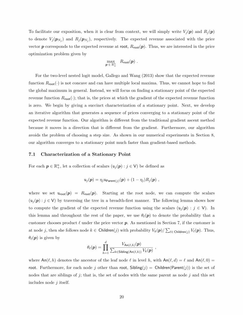
To facilitate our exposition, when it is clear from context, we will simply write Vj(p) and Rj(p)

to denote Vj(pNj ) and Rj(pNj ), respectively. The expected revenue associated with the price

vector p corresponds to the expected revenue at root, Rroot(p). Thus, we are interested in the price

optimization problem given by

maxp ∈ Rn+

Rroot(p) .

For the two-level nested logit model, Gallego and Wang (2013) show that the expected revenue

function Rroot(·) is not concave and can have multiple local maxima. Thus, we cannot hope to find

the global maximum in general. Instead, we will focus on finding a stationary point of the expected

revenue function Rroot(·); that is, the prices at which the gradient of the expected revenue function

is zero. We begin by giving a succinct characterization of a stationary point. Next, we develop

an iterative algorithm that generates a sequence of prices converging to a stationary point of the

expected revenue function. Our algorithm is different from the traditional gradient ascent method

because it moves in a direction that is different from the gradient. Furthermore, our algorithm

avoids the problem of choosing a step size. As shown in our numerical experiments in Section 8,

our algorithm converges to a stationary point much faster than gradient-based methods.

7.1 Characterization of a Stationary Point

For each p ∈ Rn+, let a collection of scalars (uj(p) : j ∈ V) be defined as

uj(p) = ηjuParent(j)(p) + (1− ηj)Rj(p) ,

where we set uroot(p) = Rroot(p). Starting at the root node, we can compute the scalars

(uj(p) : j ∈ V) by traversing the tree in a breadth-first manner. The following lemma shows how

to compute the gradient of the expected revenue function using the scalars (uj(p) : j ∈ V). In

this lemma and throughout the rest of the paper, we use θ`(p) to denote the probability that a

customer chooses product ` under the price vector p. As mentioned in Section 7, if the customer is

at node j, then she follows node k ∈ Children(j) with probability Vk(p)/∑

`∈Children(j) V`(p). Thus,

θ`(p) is given by

θ`(p) =

d∏h=1

VAn(`,h)(p)∑k∈Sibling(An(`,h)) Vk(p)

,

where An(`, h) denotes the ancestor of the leaf node ` in level h, with An(`, d) = ` and An(`, 0) =

root. Furthermore, for each node j other than root, Sibling(j) = Children(Parent(j)) is the set of

nodes that are siblings of j; that is, the set of nodes with the same parent as node j and this set

includes node j itself.

20

Lemma 7.1 (Gradient of Expected Revenue). For each p ∈ Rn+ and for every leaf node `,

∂Rroot

∂p`(p) = −θ`(p)β`

(p` −

1

β`− uParent(`)(p)

),

where θ`(p) is the probability that a customer chooses product ` under the price vector p.

We give the proof of this lemma in Online Appendix E. By using the above lemma, we can

efficiently obtain the gradient of the expected revenue at any price vector p ∈ Rn+. In particular,

we can compute the preference weight Vj(p) and the expected revenue Rj(p) for all j ∈ V, by

starting with the leaf nodes and moving up the tree in a breadth-first manner. Once we compute

the preference weights, it is straightforward to compute θ`(p) for each leaf node `. Similarly, by

using (Rj(p) : j ∈ V), we can compute (uj(p) : j ∈ V) by starting from the root node and moving

down the tree in a breadth-first manner. Once we know θ`(p) and uParent(`)(p) for each leaf node

`, the above lemma gives a closed-form expression for the gradient.

Lemma 7.1 allows us to apply the traditional gradient ascent method to compute a stationary

point of the expected revenue function; see Sun and Yuan (2006). However, in our numerical

experiments in Section 8, we observe that the traditional gradient ascent method can be relatively

slow in practice and requires a careful selection of the step size. In the rest of this section, we

develop a new algorithm for computing a stationary point of the expected revenue function. This

algorithm is different from the gradient ascent method and completely avoids the problem of step

size selection. When developing our algorithm, we make use of a succinct characterization of the

stationary points of the expected revenue function, given by the following corollary. The proof

of this corollary immediately follows from the above lemma and the fact that the probability of

choosing each product is always positive.

Corollary 7.2 (A Necessary and Sufficient Condition for a Stationary Point). For each p ∈ Rn+,

p is a stationary point of Rroot(·) if and only if p` = 1β`

+ uParent(`)(p) for all `.

7.2 A Pricing Algorithm without Gradients

By Corollary 7.2, if we can find a price vector p ∈ Rn+ such that p` = 1β`

+ uParent(`)(p) for all `,

then p corresponds to a stationary point of the expected revenue function. This observation yields

the following iterative idea to find a stationary point of the expected revenue function. We start

with a price vector p0 ∈ Rn+. In iteration s, we compute (uj(ps) : j ∈ V). Using this collection

of scalars, we compute the price vector ps+1 at the next iteration as ps+1` = 1

β`+ uParent(`)(p

s) for

each leaf node `. It turns out that a modification of this idea generates a sequence of price vectors

21

{ps ∈ Rn+ : s = 0, 1, 2, . . .} that converges to a stationary point of the expected revenue function

and it forms the basis of our pricing algorithm. We give our pricing algorithm below, which we call

the Push-Up-then-Push-Down (PUPD) algorithm.

Push-Up-then-Push-Down (PUPD):

Step 0. Set the iteration counter s = 0 and p0 = 0.

Step 1. Compute the scalars (tsj : j ∈ V) recursively over the tree as follows. For root, we have

tsroot = Rroot(ps). Using Rsj = Rj(p

s) to denote the expected revenue at node j under the price

vector ps, for the other nodes, we have

tsj = max{tsParent(j) , ηjt

sParent(j) + (1− ηj)Rsj

}.

Step 2. The price vector ps+1 at the next iteration is given by ps+1` = 1

β`+ tsParent(`) for each

leaf node `. Increase s by one and go back to Step 1.

There are several stopping criteria to consider for the PUPD algorithm. For example, we

can terminate the algorithm if ‖ps+1 − ps‖2 is less than some pre-specified tolerance. In our

numerical experiments in the next section that compare the PUPD algorithm with the gradient-

based algorithm, we use a common criterion and stop the algorithms when the norm of the gradient

of the expected revenue function ‖∇Rroot (ps) ‖2 is less than some pre-specified tolerance.

Our algorithm is called Push-Up-then-Push-Down because given the price vector ps, we compute

Rroot(ps) by “pushing up,” starting at the leaf nodes and computing the expected revenue at each

node in the tree in a breadth-first manner, until we reach root. Once we obtain (Rj(ps) : j ∈ V), we

compute (tsj : j ∈ V) by “pushing down,” starting from root and computing these scalars at each

node in the tree in a breadth-first manner. Also, we note that our PUPD algorithm is different

from the gradient ascent method because in each iteration s, the gradient of the expected revenue

function at ps is given by

∂Rroot

∂p`(p)

∣∣∣∣p=ps

= −θ`(ps)β`(ps` −

1

β`− uParent(`)(p

s)

),

whereas the change in the price vector in iteration s under our PUPD algorithm is given by

ps+1` − ps` = −(ps` −

1β`− tsParent(`)). Thus, the direction of change ps+1 − ps under our PUPD

algorithm is not necessarily parallel to the gradient of the expected revenue function at price vector

ps. The following theorem gives our main result for the PUPD algorithm and it shows that the

sequence of price vectors generated by our PUPD algorithm converges to a stationary point of the

22

expected revenue function. The proof of this theorem is given in Online Appendix E.

Theorem 7.3 (Convergence to a Stationary Point). The sequence of prices under the PUPD

algorithm converges to a stationary point of the expected revenue function Rroot(·) .

7.3 Extension to Arbitrary Cost Functions

We can extend Lemma 7.1 to the case in which there is a cost associated with offering a product and

this cost is a function of the market share of the product. In particular, we consider the problem

maxp

Π(p) ≡ Rroot(p)−n∑`=1

C`(θ`(p)) , (7)

where C`(·) denotes the cost function associated with product ` and θ`(p) denotes the probability

that a customer chooses product ` under the price vector p. The above model allows each product

` to involve a different cost C`(·).

The main result of this section provides an expression for the gradient of the profit function

Π(·). Before we proceed to the statement of the theorem, we introduce some notation. For any

nodes i and j, let θij(p) denote the probability that we can get from node i to node j; that is,

θij(p) =

m∏h=1

Vkh∑u∈Sibling(kh) Vu

if there is a (unique) path (i = k0, k1, . . . , km = j) from i to j

0 otherwise.

Note that θroot` (p) is exactly the same as θ`(p) defined just before Lemma 7.1, and thus, we can

write θroot` (p) simply as θ`(p), dropping the superscript root for convenience. For all p ∈ Rn+ and

for all leaf nodes i and `, let vi,`(p) be defined by:

vi,`(p) ≡

∑si,`

s=0

∏dh=s+1 ηAn(`,h)

θrootAn(`,s)

(p)

(1− ηAn(`,s)

)if i 6= `

− 1θroot` (p)

+∑d−1

s=0

∏dh=s+1 ηAn(`,h)

θrootAn(`,s)

(p)

(1− ηAn(`,s)

)if i = `,

where si,` = max{h : An(i, h) = An(`, h)}. Note that si,` is well-defined with 0 ≤ si,` ≤ d because

root at level 0 is a common ancestor of all nodes. Also, si,` = d if and only if i = `. Here is the

main result of this section, whose proof is given in Online Appendix E.

23

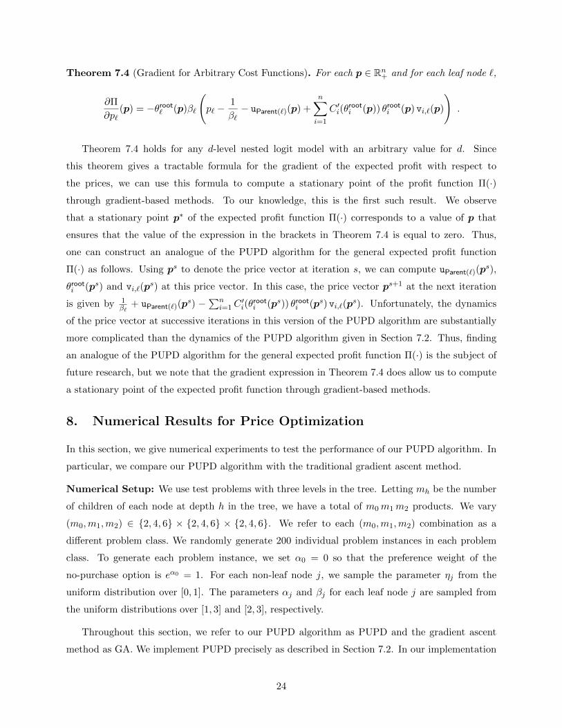
Theorem 7.4 (Gradient for Arbitrary Cost Functions). For each p ∈ Rn+ and for each leaf node `,

∂Π

∂p`(p) = −θroot` (p)β`

(p` −

1

β`− uParent(`)(p) +

n∑i=1

C ′i(θrooti (p)) θrooti (p) vi,`(p)

).

Theorem 7.4 holds for any d-level nested logit model with an arbitrary value for d. Since

this theorem gives a tractable formula for the gradient of the expected profit with respect to

the prices, we can use this formula to compute a stationary point of the profit function Π(·)

through gradient-based methods. To our knowledge, this is the first such result. We observe

that a stationary point p∗ of the expected profit function Π(·) corresponds to a value of p that

ensures that the value of the expression in the brackets in Theorem 7.4 is equal to zero. Thus,

one can construct an analogue of the PUPD algorithm for the general expected profit function

Π(·) as follows. Using ps to denote the price vector at iteration s, we can compute uParent(`)(ps),

θrooti (ps) and vi,`(ps) at this price vector. In this case, the price vector ps+1 at the next iteration

is given by 1β`

+ uParent(`)(ps) −

∑ni=1C

′i(θ

rooti (ps)) θrooti (ps) vi,`(p

s). Unfortunately, the dynamics

of the price vector at successive iterations in this version of the PUPD algorithm are substantially

more complicated than the dynamics of the PUPD algorithm given in Section 7.2. Thus, finding

an analogue of the PUPD algorithm for the general expected profit function Π(·) is the subject of

future research, but we note that the gradient expression in Theorem 7.4 does allow us to compute

a stationary point of the expected profit function through gradient-based methods.

8. Numerical Results for Price Optimization

In this section, we give numerical experiments to test the performance of our PUPD algorithm. In

particular, we compare our PUPD algorithm with the traditional gradient ascent method.

Numerical Setup: We use test problems with three levels in the tree. Letting mh be the number

of children of each node at depth h in the tree, we have a total of m0m1m2 products. We vary

(m0,m1,m2) ∈ {2, 4, 6} × {2, 4, 6} × {2, 4, 6}. We refer to each (m0,m1,m2) combination as a

different problem class. We randomly generate 200 individual problem instances in each problem

class. To generate each problem instance, we set α0 = 0 so that the preference weight of the

no-purchase option is eα0 = 1. For each non-leaf node j, we sample the parameter ηj from the

uniform distribution over [0, 1]. The parameters αj and βj for each leaf node j are sampled from

the uniform distributions over [1, 3] and [2, 3], respectively.

Throughout this section, we refer to our PUPD algorithm as PUPD and the gradient ascent

method as GA. We implement PUPD precisely as described in Section 7.2. In our implementation

24

of GA, we generate a sequence of price vectors {ps ∈ Rn+ : s = 0, 1, 2, . . .}, where ps+1 = ps +

ts∇Rroot(ps), ∇Rroot(p

s) is the gradient of the expected revenue function evaluated at ps and ts is

a step size parameter. To choose the step size parameter ts in iteration s, we find a local solution

to the problem maxt≥0Rroot(ps + t∇Rroot(p

s)) by using golden section search; see Sun and Yuan

(2006). We use the same stopping criterion for PUPD and GA, and we stop these algorithms when

the norm of the gradient satisfies ‖∇Rroot(ps)‖2 ≤ 10−6.

Numerical Results: In Table 4, we compare the running times for PUPD and GA. The first

three columns in Table 4 show the parameters of each problem class by giving (m0,m1,m2). The

fourth column shows the average number of iterations for PUPD to reach the stopping criterion,

where the average is taken over all 200 problem instances in a problem class. Similarly, the fifth

column shows the average number of iterations for GA to reach the stopping criterion. The next

three columns give various statistics regarding the ratio between the numbers of iterations for

GA and PUPD to reach the stopping criterion. To be specific, letting ItnGA(k) and ItnPUPD(k)

respectively be the numbers of iterations for GA and PUPD to stop for problem instance k in a

certain problem class, the sixth, seventh and eighth columns respectively give the average, minimum

and maximum of the figures {ItnGA(k)/ItnPUPD(k) : k = 1, . . . , 200}. Finally, the last three

columns give various statistics regarding the ratio between the running times of GA and PUPD. In

particular, letting TimeGA(k) and TimePUPD(k) respectively be the running times for GA and

PUPD to reach the stopping criterion for problem instance k in a certain problem class, the ninth,

tenth and eleventh columns in the table respectively give the average, minimum and maximum of

the figures {TimeGA(k)/TimePUPD(k) : k = 1, . . . , 200}.

The results in Table 4 indicate that PUPD takes drastically fewer iterations to reach the stopping

criterion when compared with GA. The ratio between the number of iterations for GA and PUPD

ranges between 2 to 514. This ratio never falls below one, showing that PUPD stops in fewer

iterations than GA in all problem instances. We observe that as the problem size measured by

the number of products m0m1m2 increases, the number of iterations for GA to reach the stopping

criterion tends to increase, whereas the number of iterations for PUPD remains stable and it even

shows a slightly decreasing trend. These observations suggest the superiority of PUPD especially in

larger problem instances. The last three columns in Table 4 show that, in addition to the number

of iterations, the running times for PUPD are also substantially smaller than those of GA. GA

takes at least twice as long as PUPD over all problem instances. There are problem instances, in

which the running time for GA is 466 times larger than that of PUPD. The ratios of the running

times never fall below one in any problem instance, indicating that PUPD always reaches the

25

Ratio Between Ratio BetweenPrb. Class Avg. No. Itns No. Itns. Run. Times

m0 m1 m2 PUPD GA Avg. Min Max Avg. Min Max

2 2 2 124 2,019 12 2 131 10 2 1082 2 4 112 3,393 25 5 184 21 4 1882 2 6 93 4,201 34 8 158 29 6 1412 4 2 122 5,194 36 4 230 31 3 1962 4 4 104 5,390 47 11 172 40 9 1462 4 6 95 7,117 69 16 251 60 13 2752 6 2 124 6,520 47 6 168 41 5 1392 6 4 113 8,401 72 15 235 64 13 2522 6 6 101 10,390 102 24 294 89 19 2994 2 2 161 6,470 35 4 205 31 3 2044 2 4 128 6,848 50 11 179 43 9 1594 2 6 114 9,136 77 19 236 67 16 2254 4 2 135 10,045 72 11 220 63 9 2424 4 4 101 12,147 118 25 270 106 22 2894 4 6 92 12,799 139 36 305 120 30 2814 6 2 122 13,204 110 14 303 98 12 3354 6 4 98 15,851 166 57 371 145 52 3254 6 6 85 17,913 217 73 396 191 62 4226 2 2 158 8,564 54 6 191 47 6 2156 2 4 125 10,441 83 16 212 73 13 1816 2 6 104 10,857 104 27 257 90 24 2476 4 2 125 14,912 120 25 280 106 22 3096 4 4 98 15,932 165 48 327 145 42 3436 4 6 86 18,087 217 101 419 194 81 4466 6 2 109 17,197 164 47 326 144 42 3116 6 4 87 19,896 239 102 398 213 84 4176 6 6 75 21,531 299 116 514 266 104 466

Table 4: Performance comparison between PUPD and GA.

stopping criterion faster than GA. This drastic difference between the performance of PUPD and

GA can, at least partially, be explained by using the following intuitive argument. Noting Lemma

7.1, under GA, if the current price vector is ps, then the price of product ` changes in the direction

−θ`(ps)β`(ps` −

1β`− uParent(`)(p

s))

. If the price of product ` in price vector ps is large, then the

choice probability θ`(ps) is expected to be small, which implies that the change in the price of

product ` under GA is expected to be relatively small as well. However, if the price of a product

is large, then its price has to change significantly to make a noticeable impact in the price of this

product! In contrast, under PUPD, the choice probability θ`(ps) does not come into play in a

direct way when computing the change in the prices, except in an indirect way when computing

the scalars (tsj : j ∈ V). We note that PUPD and GA can converge to different stationary points

of the expected revenue function, but over all of our problem instances, the expected revenues at

the stationary points obtained by PUPD and GA differ at most by 0.02%. We also tested the

robustness of the PUPD algorithm by using different initial prices. The results are similar to those

in Table 4. For details, the reader is referred to Online Appendix F.

Finally, we applied the PUPD algorithm on problem instances with two levels in the tree. When

there are two levels in the tree, Gallego and Wang (2013) provide a set of implicit equations that

must be satisfied by the optimal price vector. We use golden section search to numerically find a

solution to this set of equations. Similar to the stopping criterion for PUPD, we stop the golden

section search when we reach a price vector ps that satisfies ‖∇Rroot(ps)‖2 ≤ 10−6. Our numerical

26

results demonstrated that PUPD can run substantially faster than golden section search for problem

instances with larger number of products. Furthermore, over all of our problem instances, the

expected revenues at the stationary points obtained by PUPD and the golden search are essentially

equal. For the details, the reader is referred to Online Appendix F.

9. The Choice Model and the Assortment Optimization Problem

In this section, we begin by providing practical motivation for the use of the d-level nested logit

model. First, we show that this model is compatible with random utility maximization (RUM)

principle. Second, we discuss that this model is equivalent to the elimination by aspects. Third, we

provide practical situations in which the d-level nested logit model with three or more levels is used

to capture the customer choice process. Finally, we demonstrate that the predictive accuracy of the

d-level nested logit model increases as the number of levels in the tree increases. This discussion

provides practical motivation for the d-level nested logit model. Following this discussion, we explain

how the assortment and price optimization problems considered in this paper become useful when

solving large-scale revenue management problems.

Random Utility Maximization: An attractive framework for describing the choice process of

customers is to appeal to the RUM principle, where a customer associates random utilities with

the products and the no-purchase option. The customer then chooses the option that provides the

largest utility. As discussed in Section 3, if the customer is at a non-leaf node j, then she chooses

node k ∈ Children(j) with probability Vk(Sk)/∑

`∈Children(j) V`(S`). For the customer to choose the

product at product `, she needs to follow the path from root to the leaf node `. Thus, given an

assortment S = (Sj : j ∈ V), the probability that a customer chooses a product ` ∈ S is

θ`(S) =

d∏h=1

VAn(`,h)

(SAn(`,h)

)∑k∈Sibling(An(`,h)) Vk(Sk)

. (8)

The following theorem shows that the choice probability above can be obtained by appealing to

the RUM principle. The proof is given in Online Appendix G.

Theorem 9.1 (Consistency with Utility Maximization). The choice probability under the d-level

nested logit model given in (8) is consistent with the RUM principle.

Borch-Supan (1990) shows the compatibility of the two-level nested logit model with the RUM

principle; see, also, McFadden (1974). The above theorem extends the result to the d-level setting.

McFadden (1978) and Cardell (1997) discuss the consistency with the RUM principle for a general

d-level setting, but they do not provide a formal proof.

27

Elimination by Aspects Model: Theorem 9.1 provides a behavioral justification for the d-level

nested logit model by relating it to the RUM principle. Another approach to provide justification for

the d-level nested logit model is to relate it to the elimination by aspects model proposed by Tversky

(1972a,b) and Tversky and Sattath (1979). This model is widely accepted in the psychology and

marketing literature for providing a reasonable heuristic for decision making. Roughly speaking, the

elimination by aspects model works similar to a screening rule. The customer chooses an attribute,

and eliminates the alternatives that do not meet the requirements based on this attribute. She

continues in this manner until she is left with a single alternative. There is a large body of

literature that explores the equivalence between the d-level nested logit and the elimination by

aspects model. Manski and McFadden (1981) point out the equivalence between the two models

in somewhat restricted settings. Tversky and Sattath (1979), Vovsha (1997) and Train (2003) also

comment on the equivalence between the d-level nested logit and elimination by aspects models.

Batley and Daly (2006) provide a formal proof that the d-level nested logit model can be derived

by appealing to the elimination by aspects model.

Applications of Nested Logit Models with Three or More Levels: Psychologists and

marketing researchers have conducted many experiments to validate the elimination by aspects

model, and thus, providing justification for the d-level nested logit model in the process. Studies

show that consumers indeed use multiple attributes to sequentially eliminate products from their

considerations. For example, Andrews and Manrai (1998) consider scanner panel data for fabric

softeners and they find that customers screen fabric softeners based on four attributes, brand name,

size, product form and formulation. For advanced photo systems, Gilbride and Allenby (2004) show

that customers consider over 10 attributes to determine the camera system that they will purchase.

These attributes include body style, mid-roll change, operation feedback, zoom lens, view finder and

price. Pihlens (2008) models the choice among different pasta sauce options by using 16 attributes,

which include container size and type, sauce base, main ingredients and price. Waddell (1993)

uses the three-level nested logit model to capture residential location choice. The three levels in

the tree correspond to workplace, housing tenure, and residence choice. Coldren and Koppelman

(2005) find that using three levels in the nested logit model provides an improvement over two levels

when modeling demand for flight itineraries. Cervero and Duncan (2008) model rail travel adoption

for daily commute by using the nested logit model with three levels. Carson et al. (2009) use the

four-level nested logit model to represent fishing demand in Alaska. Gramlich (2009) models the

choice among different vehicle options using trees with four levels, which correspond to product

features such as vehicle segment, size, comfort level, country of origin and specific vehicle model.

28

Parameter Estimation and Predictive Accuracy as the Number of Levels d Increases:

In Online Appendix H, we show that the log-likelihood function under the d-level nested logit model

exhibits desirable concavity properties, enabling us to develop an effective estimation method. In

Online Appendix H, we exploit these concavity properties to present numerical experiments, in

which we fit the d-level nested logit model to customer choice data with progressively increasing

number of levels d in the tree. Our experiments demonstrate that the predictive accuracy improves

as the number of levels d increases. Comparing with the multinomial logit model (d = 1), two-

level models (d = 2) reduce the misclassification errors by about 9%, while with three-level models

(d = 3), the misclassification errors are reduced by 15%.

Assortment and Price Optimization Problems: Assortment and price optimization

problems considered in this paper are useful when maximizing the immediate expected revenue from

a customer but these problems also find applications when solving large-scale revenue management

problems. Consider the case in which an airline operates k flights legs. We index the flight legs by

1, . . . , k. We let ci be the capacity available on flight leg i. The airline offers n itineraries to its

customers, where an itinerary is a combination of connecting flight legs and an associated price.

We index the itineraries by 1, . . . , n. We use r` to denote the revenue associated with itinerary `.

We let ai` = 1 if itinerary ` uses flight leg i, otherwise ai` = 0. The problem takes place over a finite

selling horizon of T periods. Time period T is the beginning of the selling horizon and the flight

legs depart at time period 0. For simplicity, we assume that there is one customer arrival at each

time period. The goal of the airline is to find a policy to decide which set of itineraries to make

available to its customers to maximize the total expected revenue over the selling horizon.

We let xi be the remaining capacity on flight leg i at the beginning of a time period and

use x = (x1, . . . , xk) as the state variable. The feasible set of itineraries that can be offered at

a time period is given by F(x) = {S ⊆ {1, . . . , n} : ai` 1(` ∈ S) ≤ xi ∀ i = 1, . . . k, ` = 1, . . . , n},

where 1(·) is the indicator function. The definition of F(x) captures the fact that if we offer a set

that includes itinerary ` and itinerary ` uses flight leg i, then there has to be capacity available on

flight leg i. Thus, we can find the optimal policy by solving the dynamic program

Jt(x) = maxS⊆F(x)

∑`∈S

θ`(S)(r` + Jt−1(x−

∑ki=1 ai` ei)

)+ θ0(S)Jt−1(x)

= maxS⊆F(x)

{∑`∈S

θ`(S)(r` + Jt−1(x−

∑ki=1 ai` ei)− Jt−1(x)

)}+ Jt−1(x) , (9)

where ei is a unit vector in Rk with a one in the element corresponding to flight leg i and the

choice probability θ`(S) is driven by the d-level nested logit model. For practical airline networks

29

with large number of flight legs, the dynamic program above involves a high-dimensional state

variable. Thus, it is difficult to compute the value functions exactly. However, there exist a variety

of methods to build approximations to the value functions; see Liu and van Ryzin (2008); Zhang

and Adelman (2009). In this case, if we have an approximation Jt(·) to the value function Jt(·),

then we can replace Jt(·) in the second maximization problem above with Jt(·) and solve this

problem to find a set of itineraries to offer. To solve this problem, we observe that we can drop all

itineraries for which we do not have enough capacity to offer. Once we drop these itineraries, this

problem becomes an assortment optimization problem in which the revenue of product ` is given

by r` + Jt−1(x −∑k

i=1 ai` ei) − Jt−1(x) and we maximize the expected revenue from a customer.

Thus, if we are given approximations to the value functions, then the problem of finding a set of

itineraries to offer precisely corresponds to the assortment problem considered in this paper.

Another use of our assortment optimization problems occurs when we build a linear

programming approximation to the revenue management problem described above. To formulate

this linear program, we use the decision variable h(S) to denote the number of time periods during

which we offer the subset S of itineraries. In this case, we can use the linear program

max∑

S⊆{1,...,n}

n∑`=1

r` θ`(S)h(S) (10)

s.t.∑

S⊆{1,...,n}

n∑`=1

ai` θ`(S)h(S) ≤ ci ∀ i = 1, . . . , k

∑S⊆{1,...,n}

h(S) = T

h(S) ≥ 0 ∀S ⊆ {1, . . . , n},

to approximate the optimal expected revenue over the selling horizon; see Gallego et al. (2004);

Liu and van Ryzin (2008). Noting that∑n

`=1 r` θ`(S) is the expected revenue at a time period

during which we offer the subset S of itineraries, the objective function in the problem above

computes the total expected revenue over the selling horizon. The first set of constraints

ensures that the total expected capacity consumption on each flight leg does not exceed the

capacity availability on the flight leg, whereas the second constraint ensures that we offer

a subset of itineraries at each time period. If there are n itineraries, then the number of

decision variables in the linear program above is 2n. Thus, it is customary to solve the linear

program by using column generation. Using {µi : i = 1, . . . , k} and σ to denote the dual

variables associated with the two sets of constraints above, the reduced cost of the decision

variable h(S) is given by∑n

`=1 r` θ`(S) −∑k

i=1

∑n`=1 ai` θ`(S)µi − σ. Thus, when generating

30

columns, to find the decision variable with the largest reduced cost, we can solve the problem

maxS⊆{1,...,n}∑n

`=1 r` θ`(S)−∑k

i=1

∑n`=1 ai` θ`(S)µi = maxS⊆{1,...,n}

∑n`=1 θ`(S) (r` −

∑ki=1 ai` µi).

We observe that the last problem precisely has the same form as the assortment optimization

problem considered in this paper, where the revenue of product ` is r`−∑k

i=1 ai`µi and we find an

assortment of products to maximize the expected revenue from a customer. Thus, the assortment

optimization problem studied in this paper becomes useful when generating columns for linear

programming approximations of large-scale revenue management problems.

In the dynamic program in (9) and the linear program in (10), the prices of the itineraries are

fixed and the airline decides which set of itineraries to make available. These models have their

analogues in which the set of offered itineraries are fixed and the prices of the itineraries are decision

variables; see Gallego and van Ryzin (1997). The pricing problem studied in this paper becomes

useful when dealing with large-scale revenue management problems, in which the airline offers a

fixed set of itineraries but dynamically adjusts the prices of the offered itineraries.

10. Conclusion

We considered assortment and price optimization problems under the d-level nested logit model. We

showed how to obtain an optimal assortment, and developed an algorithm to obtain a set of prices

corresponding to a stationary point of the expected revenue function. We investigated several

motivations for the d-level nested logit model and for our assortment and pricing problems. For

future research directions, one can consider extending the PUPD algorithm for joint assortment

and price optimization, establishing connections between our assortment optimization algorithm

and the linear programming formulation for the two-level model proposed by Davis et al. (2014),

and developing assortment and pricing algorithms for the case where ηj > 1 for some nodes j ∈ V.

Acknowledgement

The authors would like to thank the Area Editor, the Associate Editor, and the three anonymous

referees for their detailed and thoughtful comments that improved the paper in many ways. We

also want to thank Han Qiu for pointing out an error in the earlier version of our manuscript, which

led to a new proof showing that the revenues under the PUPD algorithm are always bounded.

References

Andrews, R. L., and A. K. Manrai. 1998. Featured-based elimination: Model and emipiricalcomparison. European Journal of Operational Research 111 (2): 248–267.

Batley, R., and A. Daly. 2006. On the equivalence between elimination-by-aspects and generalisedextreme value models of choice behaviour. Journal of Mathematical Psychology 50 (5): 456–467.

31

Borch-Supan, A. 1990. On the compatibility of nested logit models with utility maximization.Journal of Econometrics 43 (3): 373–388.

Bront, J. M., I. Mendez Diaz, and G. Vulcano. 2009. A column generation algorithm for choice-based network revenue management. Operations Research 57 (3): 769–784.

Cardell, N. S. 1997. Variance components structures for the extreme-value and logistic distributionswith applications to models of heterogeneity. Economic Theory 13 (2): 185–213.

Carson, R. T., W. M. Hanemann, and T. C. Wegge. 2009. A nested logit model of recreationalfishing demand in Alaska. Marine Resource Economics 24 (2): 101–129.

Cervero, R., and M. Duncan. 2008. Residential self selection and rail commuting: A nested logitanalysis. Technical report, University of California, Berkeley.

Chen, K. D., and W. H. Hausman. 2000. Technical Note: Mathematical properties of the optimalproduct line selection problem using choice-based conjoint analysis. Management Science 46 (2):327–332.

Coldren, G. M., and F. S. Koppelman. 2005. Modeling the competition among air-travel itineraryshares: GEV model development. Transportation Research Part A 39 (4): 345–365.

Davis, J. M., G. Gallego, and H. Topaloglu. 2014. Assortment optimization under variants of thenested logit model. Operations Research 62 (2): 250–273.

Dong, L., P. Kouvelis, and Z. Tian. 2009. Dynamic pricing and inventory control of substituteproducts. Manufacturing & Service Operations Management 11 (2): 317–339.

Farias, V. F., S. Jagabathula, and D. Shah. 2013. A non-parametric approach to modeling choicewith limited data. Management Science 59 (2): 305–322.

Gallego, G., G. Iyengar, R. Phillips, and A. Dubey. 2004. Managing flexible products on a network.Working Paper, Columbia University.

Gallego, G., R. Ratliff, and S. Shebalov. 2011. A general attraction model and an efficientformulation for the network revenue management problem. Technical report, ColumbiaUniversity, New York, NY.

Gallego, G., and H. Topaloglu. 2012. Constrained assortment optimization for the nested logitmodel. To appear in Management Science.

Gallego, G., and G. van Ryzin. 1997. A multiproduct dynamic pricing problem and its applicationsto yield management. Operations Research 45 (1): 24–41.

Gallego, G., and R. Wang. 2013. Multi-product price optimization and competition under thenested logit model with product-differentiated price sensitivities. Operations Research 62 (2):450–461.

Gilbride, T. J., and G. M. Allenby. 2004. A choice model with conjunctive, disjunctive, andcompensatory screening rules. Marketing Science 23 (3): 391–406.

Gramlich, J. P. 2009. Gas prices and fuel efficiency in the US automobile industry: Policyimplications of endogenous product choice. Ph.D. Dissertation, Georgetown University.

Hanson, W., and K. Martin. 1996. Optimizing multinomial logit profit functions. ManagementScience 42 (7): 992–1003.

Kleinberg, J., and E. Tardos. 2005. Algorithm Design. New York: Addison Wesley.Kok, A. G., M. Fisher, and R. Vaidyanathan. 2006. Assortment planning: Review of literature and

industry practice. In Retail Supply Chain Management. New York: Springer.Kok, A. G., and Y. Xu. 2010. Optimal and competitive assortments with endogenous pricing under

hierarchical choice models. Management Science 57 (9): 1546–1563.Koppelman, F. S., and V. Sethi. 2000. Closed-form discrete-choice models. In Handbook of Transport

Modeling, ed. D. A. Hensher and K. J. Button.Li, G., and P. Rusmevichientong. 2014. A greedy algorithm for the two-level nested logit model.

Operations Research Letters 42 (5): 319–324.Li, H., and T. Huh. 2013. Pricing under the nested attraction model with a multi-stage choice

structure. INFORMS Annual Meeting, Minneapolis, MN.Li, H., and W. T. Huh. 2011. Pricing multiple products with the multinomial logit and nested logit

models: Concavity and implications. Manufacturing & Service Operations Management 13 (4):549–563.

Li, Z. 2007. A single-period assortment optimization model. Production and OperationsManagement 16 (2): 369–380.

Liu, Q., and G. J. van Ryzin. 2008. On the choice-based linear programming model for network

32

revenue management. Manufacturing and Service Operations Management 10 (2): 288–310.Luce, R. D. 1959. Individual choice behavior: A theoretical analysis. New York, NY: Wiley.Manski, C. F., and D. L. McFadden. 1981. Structural analysis of discrete data and econometric

applications. The MIT Press.McFadden, D. 1974. Conditional logit analysis of qualitative choice behavior. Frontiers in

Econometrics 1 (2): 105–142.McFadden, D. 1978. Modeling the choice of residential location. Transportation Research

Record (672): 72–77.Pihlens, D. A. 2008. The multi-attribute elimination-by-aspects model. Ph.D. Dissertation,

University of Technology Sydney.Rusmevichientong, P., D. B. Shmoys, C. Tong, and H. Topaloglu. 2013. Assortment optimization

under the multinomial logit model with random choice parameters. To appear in Production andOperations Management.

Song, J.-S., and Z. Xue. 2007. Demand management and inventory control for substitutableproducts. Working Paper, Duke University.

Sun, W., and Y. Yuan. 2006. Optimization Theory and Methods: Nonlinear Programming,Volume 1. Springer.

Talluri, K., and G. J. van Ryzin. 2004. Revenue management under a general discrete choice modelof consumer behavior. Management Science 50 (1): 15–33.

Train, K. 2003. Discrete Choice Methods with Simulation. New York, NY: Cambridge UniversityPress.

Tversky, A. 1972a. Choice-by-elimination. Journal of Mathematical Psychology 9 (4): 341–367.Tversky, A. 1972b. Elimination-by-aspect: A theory of choice. Psychological Review 79 (4): 281–

299.Tversky, A., and S. Sattath. 1979. Preference Trees. Psychological Review 86 (6): 542–573.van Ryzin, G. J., and S. Mahajan. 1999. On the relationship between inventory costs and variety

benefits in retail assortments. Management Science 45:1496–1509.Vovsha, P. 1997. Application of cross-nested logit model to mode choice in Tel Aviv, Israel

metropolitan area. Transportation Research Record 1607:6–15.Waddell, P. 1993. Exogenous workplace choice in residential location models: Is the assumption

valid? Geographical Analysis 25 (1): 65–82.Wen, C.-H., and F. S. Koppelman. 2001. The generalized nested logit model. Transportation

Research Part B 35:627–641.Zhang, D., and D. Adelman. 2009, August. An approximate dynamic programming approach to

network revenue management with customer choice. Transportation Science 43 (3): 381–394.

33

Online Appendix

A. Omitted Results in Section 4

The proofs of Proposition 4.1 and Theorem 4.2 use the next lemma, which shows the relationship

between the local problem at node j given in (4) and the same problem at its children nodes.

Lemma A.1. Consider an arbitrary non-leaf node j. Assume that for every k ∈ Children(j), there

exists a set Sk ⊆ Nk such that Vk(Sk)(Rk(Sk)− t∗Parent(k)

)≥ 0 and

Vk(Sk)(Rk(Sk)− t∗Parent(k)

)≥ Vk(S∗k)

(Rk(S

∗k)− t∗Parent(k)

). (11)

Then, letting Sj =⋃· k∈Children(j) Sk, we have

Vj(Sj)(Rj(Sj)− t∗Parent(j)

)≥ Vj(S∗j )

(Rj(S

∗j )− t∗Parent(j)

). (12)

Moreover, if the inequality in (11) is strict for some k ∈ Children(j), so is the inequality in (12).

Proof: There are two cases to consider: Rj(S∗j ) ≤ t∗Parent(j) and Rj(S

∗j ) > t∗Parent(j). First, consider

the case Rj(S∗j ) ≤ t∗Parent(j). Then, it follows from the definition of t∗j that t∗j = t∗Parent(j). By our

hypothesis, Vk(Sk)(Rk(Sk)− t∗j

)≥ 0 for all k ∈ Children(j), which implies that

Vj(Sj)1/ηj

(Rj(Sj)− t∗j

)=

∑k∈Children(j)

Vk(Sk)(Rk(Sk)− t∗j

)≥ 0 ,

where the equality follows by noting that

Vj(Sj)1/ηj =

∑k∈Children(j)

Vk(Sk) and Rj(Sj) =

∑k∈Children(j) Vk(Sk)Rk(Sk)∑

k∈Children(j) Vk(Sk).

Thus, Vj(Sj)(Rj(Sj)− t∗j

)≥ 0 ≥ Vj(S∗j )

(Rj(S

∗j )− t∗Parent(j)

), completing the first case.

Now, assume that Rj(S∗j ) > t∗Parent(j). Since Vk(Sk)

(Rk(Sk)− t∗j

)≥ Vk(S∗k)

(Rk(S

∗k)− t∗j

)for

all k ∈ Children(j), we obtain

Vj(Sj)1/ηj

(Rj(Sj)− t∗j

)=

∑k∈Children(j)

Vk(Sk)(Rk(Sk)− t∗j

)≥

∑k∈Children(j)

Vk(S∗k)(Rk(S

∗k)− t∗j

)= Vj(S

∗j )1/ηj

(Rj(S

∗j )− t∗j

),

Online Appendix – 1

where the two equalities above follow from an argument similar to the one we used in the first

case. The above expression implies that

Rj(Sj)− t∗Parent(j) ≥

[Vj(S

∗j )

Vj(Sj)

]1/ηj (Rj(S

∗j )− t∗j

)+ t∗j − t∗Parent(j)

= ηj

[Vj(S

∗j )

Vj(Sj)

]1/ηj (Rj(S

∗j )− t∗Parent(j)

)+ (1− ηj)

(Rj(S

∗j )− t∗Parent(j)

)

=

ηj [Vj(S∗j )

Vj(Sj)

]1/ηj

+ 1− ηj

(Rj(S∗j )− t∗Parent(j)

),

where the first equality follows from the fact that t∗j = ηjt∗Parent(j) + (1 − ηj)Rj(S

∗j ) because

Rj(S∗j ) > t∗Parent(j). The function x 7→ x1/ηj is convex, whose derivative at x = 1 is 1/ηj , and

thus, for all x ∈ R+, we have x1/ηj ≥ 1 + 1ηj

(x− 1). Writing this inequality as ηj x1/ηj + 1− ηj ≥ x,

and using this inequality with x = Vj(S∗j )/Vj(Sj) in the above expression, we obtain

Rj(Sj)− t∗Parent(j) ≥Vj(S

∗j )

Vj(Sj)

(Rj(S

∗j )− t∗Parent(j)

),

which yields Vj(Sj)(Rj(Sj)− t∗Parent(j)

)≥ Vj(S

∗j )(Rj(S

∗j )− t∗Parent(j)

)and completes the second

case. Finally, going through the same reasoning in the proof, it is easy to verify that if the inequality

in (11) is strict for some k, then the inequality in (12) is also strict. 2

Here is the proof of Proposition 4.1.

Proof of Proposition 4.1: We will prove the result by induction on the depth of node j. The result

is trivially true at root because the local problem at root is identical to the assortment problem in

(3). Now, assume that the result is true for all nodes at depth h. We want to show that the result

also holds for all nodes at depth h+ 1. Suppose, on the contrary, that there exists node i at depth

h+ 1 such that

Vi(S∗i )(Ri(S

∗i )− t∗Parent(i)

)< max

Si⊆NiVi(Si)

(Ri(Si)− t∗Parent(i)

),

and let Si ⊆ Ni be the set that achieves the maximum on the right side above. By our construction,

we have that Vi(Si)(Ri(Si)− t∗Parent(i)

)≥ 0 because an empty set yields a value of zero for the

optimization problem on the right side above. Also,

Vi(Si)(Ri(Si)− t∗Parent(i)

)> Vi(S

∗i )(Ri(S

∗i )− t∗Parent(i)

).

Online Appendix – 2

We use j to denote the parent of node i. For each k ∈ Children(j), let Sk be defined by:

Sk =

Si if k = i

arg maxSk⊆Nk Vi(Sk)(Rk(Sk)− t∗j

)if k 6= i .

By our construction, for every k ∈ Children(j),

Vk(Sk)(Rk(Sk)− t∗Parent(k)

)≥ Vk(S

∗k)(Rk(S

∗k)− t∗Parent(k)

),

and the inequality above is strict if k = i. Letting Sj =⋃· k∈Children(j) Sk, it then follows from

Lemma A.1 that

Vj(Sj)(Rj(Sj)− t∗Parent(j)

)> Vj(S

∗j )(Rj(S

∗j )− t∗Parent(j)

).

Since node j is at depth h, by the inductive hypothesis, S∗j solves the local problem at node j,

yielding

Vj(S∗j )(Rj(S

∗j )− t∗Parent(j)) = max

Sj⊆NjVj(Sj)

(Rj(Sj)− t∗Parent(j)

).

The above equality contradicts the last inequality! Therefore, the result must also hold for all nodes

at depth h+ 1, as desired. 2

Below is the proof of Theorem 4.2.

Proof of Theorem 4.2: Because of the hypothesis of the theorem, since Sk solves the local problem

at node k, we must have Vk(Sk)(Rk(Sk)− t∗Parent(k)

)≥ 0 because the empty set gives an objective

value of zero for the local problem at node k and Sk is an optimal solution to the local problem at

node k. Also, by definition of Sk, for every k ∈ Children(j),

Vk(Sk)(Rk(Sk)− t∗Parent(k)

)≥ Vk(S∗k)

(Rk(S

∗k)− t∗Parent(k)

).

Let Sj =⋃· k∈Children(j) Sk. It then follows from Lemma A.1 that

Vj(Sj)(Rj(Sj)− t∗Parent(j)

)≥ Vj(S∗j )

(Rj(S

∗j )− t∗Parent(j)

)= max

Sj⊆NjVj(Sj)

(Rj(Sj)− t∗Parent(j)

),

where the last equality follows from Proposition 4.1. This completes the proof. 2

Online Appendix – 3

B. Omitted Results in Section 5

Below, we give the proof of Theorem 5.2.

Proof of Theorem 5.2: We will prove by induction that for each h = 0, 1, 2, . . . , d,

∑j∈V : depth(j)=h

|Aj | ≤ 2n ,

where depth(j) denotes the depth of node j. The result is true for h = d because for each leaf node

j, Aj = {{j},∅}. Suppose the result is true for h + 1. Consider nodes at level h. It follows from

Lemma 5.1 that

∑j∈V : depth(j)=h

|Aj | ≤∑

j∈V : depth(j)=h

∑k∈Children(j)

|Ak| =∑

j∈V : depth(j)=h+1

|Aj | ≤ 2n ,

where the last inequality follows from the inductive hypothesis. Therefore, the total running time

of the algorithm is

d∑h=0

∑j∈V : depth(j)=h

|Aj | log (|Aj |) ≤d∑

h=0

∑j∈V : depth(j)=h

|Aj |

× log

∑j∈V : depth(j)=h

|Aj |

≤

d∑h=0

2n log(2n) = 2(d+ 1)n log(2n) = O(dn log n) ,

which completes the proof. 2

C. Practical Performance of Assortment Optimization Algorithm

We test the practical performance of our assortment optimization algorithm by applying it on

test problems with two and three levels in the tree. To our knowledge, our algorithm is the only

efficient approach for solving the assortment problem when there are three levels in the tree. For

the test problems with three levels, we compare our assortment optimization algorithm with a full

enumeration scheme that checks the expected revenue from every possible assortment. For the test

problems with two levels, Davis et al. (2014) show that the optimal assortment can be obtained

by solving a linear program. For the test problems with two levels, we compare our assortment

optimization algorithm with the full enumeration scheme and the linear programming approach

in Davis et al. (2014). We refer to our assortment optimization algorithm, the full enumeration

scheme and the linear programming approach as AA, FE and LP, respectively.

Online Appendix – 4

For the test problems with three levels, we use mh to denote the number of children of each

node at depth h and we vary (m0,m1,m2) over {2, 4, 8} × {2, 4, 8} × {2, 4, 8}. Therefore, smallest

problem instances have 23 = 8 products, whereas largest ones have 83 = 512 products. We refer to

each combination of (m0,m1,m2) as a problem class. In each problem class, we randomly generate

200 problem instances. To generate each problem instance, we sample the parameters rj and vj for

each leaf node from the uniform distribution over [0, 5] and the parameter ηj for each non-leaf node

from the uniform distribution over [0, 1]. We use the same approach to generate the test problems

with two levels, but we vary (m0,m1) over {2, 4, 8} × {2, 4, 8}.

Table 5 gives our results. In the left portion of the table, the first three columns show the

parameters (m0,m1,m2) for each problem class with three levels. The next two columns show

the running times for AA and FE, averaged over 200 problem instances in a particular problem

class. When the number of products exceeds 16, FE is not able to check the expected revenues

from all 2n assortments in a reasonable amount of time. For such problem instances, since the

number of operations required to compute the expected revenue from each assortment is the same,

we check the expected revenues from 1,000 randomly sampled assortments and linearly extrapolate

the running time for checking the expected revenues from all 2n assortments. The format of the

right portion of Table 5 is similar to that of the left portion, but the right portion focuses on the

test problems with two levels and gives the average running times for AA, FE and LP.

Considering the test problems with three levels in the left portion of Table 5, our results indicate

that the running time for AA can be substantially faster than the running time for FE. For the

problem class (2, 2, 2), which involves the smallest number of products, the average running times

for AA and FE are comparable. For all other problem classes, the average running time for AA is

smaller than the average running time for FE by orders of magnitude. The running time of AA is

reasonable. Even for the largest problem instances with 512 products, the average running time for

AA is slightly above one second. Over all of our test problems, the number of assortments in the

collection Aroot constructed by AA is roughly equal to the number of products. Considering the test

problems with two levels in the right portion of Table 5, our results indicate that the running time for

LP is generally faster than the running time for AA. For a two-level tree with m0 and m1 child nodes

in the two levels of the tree, there are m0m1 products and the linear program proposed by Davis

et al. (2014) has O(m0) decision variables and O(m0m1) constraints. The number of operations

required to solve a general linear program of this size is O(m40m1). In contrast, Theorem 5.2 shows

that AA requires O(m0m1 log(m0m1)) operations. So, the computational complexity for AA is

better than the computational complexity for solving the linear program used by LP, but many

Online Appendix – 5

Prb. Class Avg. Secs. Avg. Secs.m0 m1 m2 for AA for FE

2 2 2 1.64 ×10−2 9.50 ×10−3

2 2 4 2.29 ×10−2 2.49 ×100

2 2 8 3.17 ×10−2 1.57 ×105

2 4 2 3.05 ×10−2 2.47 ×100

2 4 4 5.23 ×10−2 1.84 ×105

2 4 8 7.35 ×10−2 7.07 ×1014

2 8 2 7.94 ×10−2 1.68 ×105

2 8 4 1.30 ×10−1 7.24 ×1014

2 8 8 2.21 ×10−1 1.40 ×1034

4 2 2 2.96 ×10−2 2.50 ×100

4 2 4 4.17 ×10−2 1.65 ×105

4 2 8 6.75 ×10−2 7.13 ×1014

4 4 2 5.89 ×10−2 1.67 ×105

4 4 4 9.68 ×10−2 7.33 ×1014

4 4 8 1.60 ×10−1 1.39 ×1034

4 8 2 1.62 ×10−1 7.64 ×1014

4 8 4 2.70 ×10−1 1.47 ×1034

4 8 8 4.72 ×10−1 5.36 ×1072

8 2 2 6.83 ×10−2 1.71 ×105

8 2 4 1.05 ×10−1 7.41 ×1014

8 2 8 1.71 ×10−1 1.40 ×1034

8 4 2 1.41 ×10−1 7.84 ×1014

8 4 4 2.38 ×10−1 1.55 ×1034

8 4 8 3.94 ×10−1 5.37 ×1072

8 8 2 3.86 ×10−1 1.63 ×1034

8 8 4 6.32 ×10−1 5.91 ×1072

8 8 8 1.10 ×100 7.76 ×10149

Prb. Class Avg. Secs. Avg. Secs. Avg. Secs.m0 m1 for AA for FE for LP

2 2 8.41 ×10−3 3.77 ×10−4 2.94 ×10−3

2 4 1.11 ×10−2 5.10 ×10−3 3.00 ×10−3

2 8 1.14 ×10−2 1.02 ×100 3.03 ×10−3

4 2 1.32 ×10−2 5.10 ×10−3 3.03 ×10−3

4 4 1.98 ×10−2 1.15 ×100 3.17 ×10−3

4 8 2.77 ×10−2 7.59 ×104 3.25 ×10−3

8 2 3.63 ×10−2 1.19 ×100 3.26 ×10−3

8 4 5.44 ×10−2 7.36 ×104 3.18 ×10−3

8 8 8.16 ×10−2 3.16 ×1014 3.42 ×10−3

Table 5: Running times for AA, FE and LP for the test problems with two and three levels.

constraints of the linear program used by LP have only two non-zero entries and it appears that

linear programming software can effectively exploit this sparse structure to obtain quite satisfactory

running times for LP. For these problem instances, we observe that LP is faster than the greedy

algorithm in Li and Rusmevichientong (2014). Thus, our results indicate that LP is a strong

approach when the tree has two levels, but we emphasize that LP cannot deal with trees with more

than two levels. For small test problems with four or eight products, the running times for FE can

be competitive to the running times for AA, but the running times for FE quickly deteriorate as

the number of products increases.

D. Extension to Multi-Period Capacity Allocation

In this section, we discuss the extension of our results to the multi-period capacity allocation model

of Talluri and van Ryzin (2004). The model of Talluri and van Ryzin (2004) is one of the pioneering

works demonstrating the importance of incorporating choice behavior into operational decisions.

Let us briefly review the setup for this problem. We have an initial capacity of C seats on a flight

leg that must be allocated over T periods. There are n products (fare classes) that can be offered

to customers, indexed by {1, . . . , n}. If we sell one ticket for fare class `, then we generate a revenue

Online Appendix – 6

of r`. In each period, based on the remaining capacity, we must find an assortment of fare classes

to offer to an arriving customer, who chooses a fare class from the assortment according to the

d-level nested logit model. The goal is to determine the revenue-maximizing policy for offering

assortments of fare classes over the selling horizon. For simplicity, we assume that there is exactly

one customer arriving in each period, but all of our results extend to the case in which there is a

positive probability that no customer shows up in a period.

We show that, under the d-level nested logit model, a nested control policy is optimal. In other

words, we show that as we have less remaining capacity in a period, we offer a smaller assortment

of fare classes. An important managerial implication of this result is that the optimal control policy

can be implemented by using protection levels, which is the standard tool in traditional revenue

management systems. That is, for each fare class `, there exists a protection level c∗`t such that

if the remaining capacity in period t is less than c∗`t, then it is optimal not to make fare class `

available in this period. Due to the optimality of a protection level policy, the d-level nested logit

model can be easily integrated with the existing revenue management controls.

To establish the optimality of a nested control policy, for each x ∈ {0, 1, . . . , C}, let Jt(x) denote

the maximum expected revenue when we have x units of capacity and t periods remaining in the

selling horizon. Under the d-level nested logit model, if we offer the assortment S of fare classes,

then the probability that a customer chooses fare class ` is θ`(S) as given in (8). In this case, Jt(·)

satisfies the dynamic programming equation

Jt(x) = maxS⊆{1,...,n}

∑`∈S

θ`(S) (r` + Jt−1(x− 1)) + θ0(S)Jt−1(x)

= maxS⊆{1,...,n}

{∑`∈S

θ`(S) (r` −∆Jt−1(x))

}+ Jt−1(x) ,

where ∆Jt−1(x) = Jt−1(x) − Jt−1(x − 1) denotes the marginal value of capacity. The boundary

conditions of the dynamic program are J0(x) = 0 for all x and Jt(0) = 0 for all t. Let S∗t (x) denote

the optimal solution in the last problem on the right side above, corresponding to the optimal

assortment to offer when we have x units of remaining inventory and t periods to go. The main

result of this section is stated in the following theorem.

Theorem D.1 (Nested Policy). For the multi-period capacity allocation problem, there exists

an optimal policy such that for each t, S∗t (x) is non-decreasing in x, satisfying S∗t (x − 1) ⊆

S∗t (x). Moreover, for each x, S∗t (x) is non-increasing in t, satisfying St(x) ⊆ St−1(x).

The first part of the above theorem shows that we offer a smaller assortment when we have less

Online Appendix – 7

capacity in a period. In this case, letting c∗`t be the smallest x such that ` ∈ S∗t (x), if the remaining

capacity in period t is less than c∗`t, then it is optimal not to offer fare class ` in this period. Therefore,

we can implement the resulting optimal policy by using protection level policies. On the other hand,

the second part of the above theorem shows that we offer a larger assortment when we have fewer

periods remaining in the selling horizon.

We define some additional notation to prove Theorem D.1. For each δ ≥ 0 and each assortment

S, let f δ(S) denote the expected revenue under assortment S = (Sj : j ∈ V) when the revenue of

every product is increased by δ; that is,

f δ(S) ≡∑`∈S

(r` + δ)θ`(S) =∑`∈S

r` θ`(S) + δ∑`∈S

θ`(S) = f0(S) + δ∑`∈S

θ`(S) ,

and let Sδ denote an assortment that maximizes f δ(·); that is, Sδ = arg maxS⊆{1,...,n} fδ(S).

The proof of Theorem D.1 uses lemmas that establish properties of the collection Aj in the

assortment optimization algorithm in Section 5. Throughout this section, we recall that Sk(u) is

an optimal solution to problem (5) and the collection of subsets Aj is constructed as in (6). In the

next lemma, we show that the subsets in the collection Aj can be ordered such that one subset is

included in another one, naturally with the exception of the largest subset. This lemma becomes

useful in the proof of Lemma D.4.

Lemma D.2. For any node j, consider the collection Aj = {Sqj : q = 1, . . . , Qj} constructed as in

(6). The subsets in this collection can be ordered such that S1j ⊆ S2

j ⊆ . . . ⊆ SQjj .

Proof. We show the result by induction on the depth of node j. For leaf node j, we have Aj =

{∅, {j}}. Since ∅ ⊆ {j}, the result holds for leaf nodes. Assume that the result holds for all nodes

at depth h+1 and consider node j at depth h. By the inductive hypothesis, for all k ∈ Children(j),

the subsets in Ak can be ordered such that S1k ⊆ S2

k ⊆ . . . ⊆ SQkk . For all k ∈ Children(j), we claim

that the optimal solution to problem (5) becomes a larger subset as u gets smaller.

Claim 1: Letting Sk(u) be an optimal solution to problem (5), if u > u′, then Sk(u) ⊆ Sk(u′).

By the definition of Sk(u), we have Vk(Sk(u)) (Rk(Sk(u) − u) ≥ Vk(Sk(u′)) (Rk(Sk(u

′) − u)

and Vk(Sk(u′)) (Rk(Sk(u

′)− u′) ≥ Vk(Sk(u)) (Rk(Sk(u)− u′). Adding these two inequalities yields

Vk(Sk(u′)) (u − u′) ≥ Vk(Sk(u)) (u − u′). Using u > u′, we get Vk(Sk(u

′)) ≥ Vk(Sk(u)). Noting

problem (5), Sk(u) and Sk(u′) are both in Ak by definition and since the subsets in the collection

Ak satisfy S1k ⊆ S2

k ⊆ . . . ⊆ SQkk by the inductive hypothesis, we must have either Sk(u) ⊆ Sk(u′)

or Sk(u) ⊇ Sk(u′). Since we have Vk(Sk(u

′)) ≥ Vk(Sk(u)), the preference weight under the subset

Online Appendix – 8

Sk(u′) is larger. Thus, the subset Sk(u

′) must be larger than Sk(u), establishing the claim.

By the claim above, Sk(u) ⊆ Sk(u′) for all k ∈ Children(j), so that

⋃· k∈Children(j) Sk(u) ⊆⋃

· k∈Children(j) Sk(u′). By (6), Aj is constructed asAj =

{⋃· k∈Children(j) Sk(u) : u ∈ R

}, so the subsets

in the collection Aj can be ordered such that one subset includes the other one, as desired. 2

By Claim 1 in Section 5, the collection Aj includes an optimal solution to the local problem at

node j. In the next lemma, we show that the collection Aj still includes an optimal solution to the

local problem at node j even after increasing the revenues associated with the products by δ.

Lemma D.3. For any node j, consider the collection Aj constructed as in (6). This collection

includes an optimal solution to the local problem at node j even when we increase the revenues

associated with the products by any δ ≥ 0.

Proof. The solution to the local problem at a leaf node j is always either {j} or ∅. Thus, Aj =

{{j},∅} always includes an optimal solution to the local problem at a leaf node j. Consider a

non-leaf node j. For each k ∈ Children(j), we use Rδk(Sk) to denote the expected revenue obtained

from a customer at node k given that we offer the assortment S = (S` : ` ∈ V) and we increase the

revenues of the products by δ. Since the expected revenue at each node is a convex combination

of the product revenues, it follows that Rδk(Sk) = Rk(Sk) + δ. In this case, when we increase the

revenues of the products by δ, the local problem at node k is given by

maxSk⊆Nk

Vk(Sk)(Rδk(Sk)− tδParent(k)

)= max

Sk⊆NkVk(Sk)

(Rk(Sk)− (tδParent(k) − δ)

).

In the expression above, letting Sδ = (Sδ` : ` ∈ V) be an optimal solution to problem (3) when we

increase the revenues of the products by δ, the scalars (tδj : j ∈ V) are given by

tδj = max{tδParent(j) , ηj t

δParent(j) + (1− ηj)Rδj(Sδj )

},

with the convention that tδParent(root) = 0. Comparing the problem above with (5) and noting that

we use Sk(u) to denote an optimal solution to problem (5), it follows that Sk(tδParent(k) − δ) is an

optimal solution to the local problem at node k when we increase the revenues of the products by

δ. In this case, by Theorem 4.2,⋃· k∈Children(j) Sk(t

δParent(k) − δ) is an optimal solution to the local

problem at node j when we increase the revenues of the products by δ. By (6), Aj is constructed

as Aj ={⋃· k∈Children(j) Sk(u) : u ∈ R

}, so

⋃· k∈Children(j) Sk(t

δParent(k) − δ) ∈ Aj . Thus, it follows

that the collection Aj includes an optimal solution to the local problem at node j even when we

increase the revenues of the products by any δ. 2

Online Appendix – 9

The next lemma shows that when we increase the revenues of the products by a positive constant,

the optimal assortment becomes larger.

Lemma D.4 (Larger Revenues Lead to Larger Assortments). For all δ ≥ 0, S0 ⊆ Sδ.

Proof. By Lemma D.3, the collection Aroot includes an optimal solution to the local problem at

root when we increase the revenues of the products by any amount δ ≥ 0. Furthermore, the local

problem at root is equivalent to the assortment problem that we want to solve. Thus, noting that

S0 is the optimal assortment and Sδ is the optimal assortment when we increase the revenues of

the products by δ, both S0 and Sδ are in Aroot. On the other hand, by Lemma D.2, if S0 and Sδ

are in Aroot, then we must have S0 ⊆ Sδ or Sδ ⊆ S0. Given an assortment S = (Sj : j ∈ V), we

use θ`(S) to denote the probability that a customer purchases product ` under the d-level nested

logit model. By the definitions of S0 and Sδ, we have∑

`∈S0 θ`(S0) r` ≥

∑`∈Sδ θ`(S

δ) r` and∑`∈Sδ θ`(S

δ) (r` + δ) ≥∑

`∈S0 θ`(S0) (r` + δ). Adding these two inequalities yields

∑`∈Sδ θ`(S

δ) ≥∑`∈S0 θ`(S

0), indicating that when we offer the assortment Sδ, the probability that a customer

purchases a product within this assortment is larger when compared with the case when we offer

the assortment S0. It is straightforward to check that under the d-level nested logit model, if

we offer a larger assortment, then the probability that a customer makes a purchase within this

assortment gets larger. At the beginning of the proof, we show that we have either S0 ⊆ Sδ or

Sδ ⊆ S0. Thus, noting that the probability that a customer makes a purchase is larger when we

offer the assortment Sδ, it must the case that S0 ⊆ Sδ. 2

Proof of Theorem D.1

Proof. Lemmas 4 and 5 in Talluri and van Ryzin (2004) show that the value functions are concave

in the remaining capacity and the first differences of the value functions decrease as we approach the

end of the selling horizon; that is, ∆Jt(x) ≤ ∆Jt(x− 1) and ∆Jt(x) ≥ ∆Jt−1(x) for t = 1, 2, . . . , T

and x = 1, 2, . . . , C. To show that S∗t (x− 1) ⊆ S∗t (x), by definition, we have

S∗t (x) = arg maxS⊆{1,...,n}

∑`∈S

θ`(S) (r` −∆Jt−1(x− 1) + ∆Jt−1(x− 1)−∆Jt−1(x))

S∗t (x− 1) = arg maxS⊆{1,...,n}

∑`∈S

θ`(S) (r` −∆Jt−1(x− 1)) .

Let δ = ∆Jt−1(x − 1) − ∆Jt−1(x). Note that δ ≥ 0 since ∆Jt(x) ≤ ∆Jt(x − 1). Thus, applying

Lemma D.4, with S0 = S∗t (x − 1) and Sδ = S∗t (x), yields S∗t (x − 1) ⊆ S∗t (x), as desired. To show

Online Appendix – 10

that S∗t (x) ⊆ S∗t−1(x), by definition, we have

S∗t (x) = arg maxS⊆{1,...,n}

∑`∈S

θ`(S) (r` −∆Jt−1(x))

S∗t−1(x) = arg maxS⊆{1,...,n}

∑`∈S

θ`(S) (r` −∆Jt−1(x) + ∆Jt−1(x)−∆Jt−2(x)) .

Let δ = ∆Jt−1(x) − ∆Jt−2(x), which is non-negative since ∆Jt−1(x) ≥ ∆Jt−2(x). Applying

Lemma D.4 with S0 = S∗t (x) and Sδ = S∗t−1(x) yields S∗t (x) ⊆ S∗t−1(x), as desired. 2

E. Omitted Results in Section 7

E.1 Proof of Lemma 7.1

Proof. For each node j ∈ V, let Fj(·) : Rn+ × Rn+ → R be defined by: for each p ∈ Rn+ and q ∈ Rn+,

Fj(p, q) = Vj(p)(Rj(p)− uParent(j)(q)

),

with the convention that uParent(root)(·) = 0. Since ηroot = 0, we have Vroot(p) = 1 by noting the

definition of Vj(p), in which case, Froot(p, q) = Rroot(p) for all p, q ∈ Rn+. At any price vector p,

we will now show that for every non-leaf node j and product ` that is a descendant of j, we have

∂Fj∂p`

(p, q)

∣∣∣∣(p,q)=(p,p)

=Vj(p)∑

k∈Children(j) Vk(p)× ∂Fi∂p`

(p, q)

∣∣∣∣(p,q)=(p,p)

,

where i is the child of j that is the ancestor of `. To see this, note that if we let Gk(p) = Vk(p)Rk(p),

then we have

Fj(p, q) =

∑k∈Children(j)

Vk(p)

ηj (∑k∈Children(j)Gk(p)∑k∈Children(j) Vk(p)

− uParent(j)(q)

).

By definition, among (Vk(p) : k ∈ Children(j)), only Vi(p) depends on p`. Similarly, among

(Rk(p) : k ∈ Children(j)), only Ri(p) depends on p`. Thus, differentiating the expression above

Online Appendix – 11

with respect to p`, it follows that

∂Fj∂p`

(p, q) = ηj

∑k∈Children(j)

Vk(p)

ηj−1

× ∂Vi∂p`

(p)×

(∑k∈Children(j)Gk(p)∑k∈Children(j) Vk(p)

− uParent(j)(q)

)

+

∑k∈Children(j)

Vk(p)

ηj

×

∂Gi∂p`

(p)∑

k∈Children(j) Vk(p)− ∂Vi∂p`

(p)∑

k∈Children(j)Gk(p)(∑k∈Children(j) Vk(p)

)2

=

∑k∈Children(j)

Vk(p)

ηj−1

× ∂Vi∂p`

(p)×(ηjRj(p)− ηjuParent(j)(q)

)

+

∑k∈Children(j)

Vk(p)

ηj−1

×

[∂Gi∂p`

(p)∑

k∈Children(j) Vk(p)− ∂Vi∂p`

(p)∑

k∈Children(j)Gk(p)∑k∈Children(j) Vk(p)

],

where the second equality uses the fact that Rj(p) =∑

k∈Children(j)Gk(p)/∑

k∈Children(j) Vk(p).

Using this identity once more, we can continue the chain of equalities above as

∂Fj∂p`

(p, q) =

∑k∈Children(j)

Vk(p)

ηj−1

× ∂Vi∂p`

(p)×(ηjRj(p)− ηjuParent(j)(q)

)

+

∑k∈Children(j)

Vk(p)

ηj−1

×[∂Gi∂p`

(p)− ∂Vi∂p`

(p)×Rj(p)

]

=

∑k∈Children(j)

Vk(p)

ηj−1

×{∂Gi∂p`

(p)− ∂Vi∂p`

(p)[ηjuParent(j)(q) + (1− ηj)Rj(p)

]}.

Therefore, noting that ηjuParent(j)(p) + (1 − ηj)Rj(p) = uj(p) by definition, the expression above

yields

∂Fj∂p`

(p, q)

∣∣∣∣(p,q)=(p,p)

=

∑k∈Children(j)

Vk(p)

ηj−1

×

{∂Gi∂p`

(p)

∣∣∣∣p=p

− uj(p)∂Vi∂p`

(p)

∣∣∣∣p=p

}.

By definition, we have Fi(p, q) = Gi(p) − uj(q)Vi(p), which implies that ∂Fi∂p`

(p, q) = ∂Gi∂p`

(p) −

uj(q)∂Vi∂p`(p) , and thus,

∂Fj∂p`

(p, q)

∣∣∣∣(p,q)=(p,p)

=

∑k∈Children(j)

Vk(p)

ηj−1

× ∂Fi∂p`

(p, q)

∣∣∣∣(p,q)=(p,p)

=Vj(p)∑

k∈Children(j) Vk(p)× ∂Fi∂p`

(p, q)

∣∣∣∣(p,q)=(p,p)

,

Online Appendix – 12

which is the desired result. To complete the proof, we recursively apply the above result starting

at the root node. Recalling that Froot(p, q) = Rroot(p) for all p, q ∈ Rn+, we obtain

∂Rroot

∂p`(p)

∣∣∣∣p=p

=∂Froot

∂p`(p, q)

∣∣∣∣(p,q)=(p,p)

=Vroot(p)∑

k∈Children(root) Vk(p)×∂FAn(`,1)

∂p`(p, q)

∣∣∣∣(p,q)=(p,p)

=1∑

k∈Children(root) Vk(p)×∂FAn(`,1)

∂p`(p, q)

∣∣∣∣(p,q)=(p,p)

,

where the second equality follows by ηroot = 0 so that Vroot(p) = 1. We continue the chain of

inequalities above by replacing the last partial derivative by its equivalent expression to get

∂Rroot

∂p`(p)

∣∣∣∣p=p

=1∑

k∈Children(root) Vk(p)×

VAn(`,1)(p)∑k∈Children(An(`,1)) Vk(p)

×∂FAn(`,2)

∂p`(p, q)

∣∣∣∣(p,q)=(p,p)

=VAn(`,1)(p)∑

k∈Sibling(An(`,1)) Vk(p)× 1∑

k∈Sibling(An(`,2))) Vk(p)×∂FAn(`,2)

∂p`(p, q)

∣∣∣∣(p,q)=(p,p)

.

Iteratively applying the same argument, we have that

∂Rroot

∂p`(p)

∣∣∣∣p=p

=

(d−1∏h=1

VAn(`,h)(p)∑k∈Sibling(An(`,h)) Vk(p)

)× 1∑

k∈Sibling(`) Vk(p)× ∂F`∂p`

(p, q)

∣∣∣∣(p,q)=(p,p)

.

Finally, note that F`(p, q) = V`(p`)(p` − uParent(`)(q)) = eα`−β`p`(p` − uParent(`)(q)

), which yields

∂F`∂p`

(p, q) = −β`eα`−β`p`(p` − uParent(`)(q)

)+ eα`−β`p` = −β`V`(p`)

(p` −

1

β`− uParent(`)(q)

).

Thus,

∂Rroot

∂p`(p)

∣∣∣∣p=p

= −β`

(d∏

h=1

VAn(`,h)(p)∑k∈Sibling(An(`,h)) Vk(p)

)(p` −

1

β`− uParent(`)(p)

),

and the desired result follows by noting that the product on the right side above gives θ`(p). 2

E.2 Proof of Theorem 7.3

In the rest of this section, we give a proof for Theorem 7.3 by using a series of lemmas. The

following lemma gives an upper bound on tsj for each non-leaf node j in each iteration s of the

PUPD algorithm.

Lemma E.1. Let V = V \ {1, 2, . . . , n, root} denote the set of non-leaf nodes, after excluding root,

Online Appendix – 13

and let ηmin = minj∈V

ηj. Then, for any non-leaf node j in level h and for all s,

tsj ≤ tsroot +(

1− (ηmin)h)Qs ,

where Qs = max

{tsroot, max

j∈Vtsj , max

j∈VRsj

}.

Proof: The result is trivially true for root. If j is a non-leaf node in level 1, then by definition,

tsj = max{tsroot, ηjt

sroot + (1− ηj)Rsj

}= ηjt

sroot + (1− ηj) max

{tsroot, R

sj

}≤ tsroot + (1− ηmin)Qs ,

where the last inequality follows from the definition of ηmin and Qs. Suppose the result is true for

all non-leaf nodes in level h− 1. For any non-leaf node j in level h,

tsj = max{tsParent(j), ηjt

sParent(j) + (1− ηj)Rsj

}= ηjt

sParent(j) + (1− ηj) max

{tsParent(j), R

sj

}≤ ηj

(tsroot +

(1− (ηmin)h−1

)Qs)

+ (1− ηj)Qs

= ηjtsroot +

(1− ηj (ηmin)h−1

)Qs

≤ tsroot +(

1− (ηmin)h)Qs ,

where the fist inequality follows from the inductive hypothesis and the definition of Qs. This

completes the proof. 2

The following lemma establishes a relationship between the expected revenues in consecutive

iterations of the PUPD algorithm. Its proof follows from an argument similar to the one in the

proof of Lemma A.1.

Lemma E.2. Assume that the price vectors {ps : s = 0, 1, 2, . . .} are generated by the PUPD

algorithm. For each non-leaf node j, we have

Rs+1j ≥ 1

ηj

(ηj +

V sj

V s+1j

− 1

)(Rsj − tsj

)++ tsj ,

where V sj = Vj (ps) and V s+1

j = Vj(ps+1

).

Proof: We will prove the result by induction on the depth of node j, starting with nodes at depth

d − 1. If node j is at depth d − 1, then it is the parent of a leaf node. Note the inequality in the

Online Appendix – 14

lemma is trivially true if Rsj ≤ tsj . In particular, by our construction of the PUPD algorithm, for

each ` ∈ Children(j), ps+1` ≥ tsParent(`) = tsj , in which case, since Rs+1

j is a convex combination of

(ps+1` : ` ∈ Nj), we have Rs+1

j ≥ tsj and the lemma follows. So, assume that Rsj > tsj . By definition

of the PUPD algorithm, for each ` ∈ Children(j), ps+1` = 1

β`+ tsj = arg maxx≥0 V`(x)

(x− tsj

), so

for each ` ∈ Children(j),

V s+1`

(Rs+1` − tsj

)≥ V s

`

(Rs` − tsj

).

Adding this inequality above over all ` ∈ Children(j), we get ∑`∈Children(j)

V s+1`

(Rs+1j − tsj

)=

∑`∈Children(j)

V s+1`

(Rs+1` − tsj

)

≥∑

`∈Children(j)

V s`

(Rs` − tsj

)=

∑`∈Children(j)

V s`

(Rsj − tsj),

where the two equalities above use the fact thatRs+1j =

∑k∈Children(j) V

s+1k Rs+1

k /∑

k∈Children(j) Vs+1k

and Rsj =∑

k∈Children(j) VskR

sk/∑

k∈Children(j) Vsk . Noting that V s+1

j =(∑

k∈Children(j) Vs+1j

)ηjand

V sj =

(∑k∈Children(j) V

sj

)ηj, we write the above inequality as

(V s+1j

)1/ηj (Rs+1j − tsj

)≥(V sj

)1/ηj (Rsj − tsj)

=(V sj

)1/ηj (Rsj − tsj)+

,

which implies that

Rs+1j ≥

(V sj

V s+1j

)1/ηj (Rsj − tsj

)++ tsj ≥

1

ηj

(ηj +

V sj

V s+1j

− 1

)(Rsj − tsj

)++ tsj ,

where the last inequality follows from the fact that the function q 7→ q1/ηj is convex whose derivative

at 1 is 1/ηj , and thus, q1/ηj ≥ 1 + 1ηj

(q − 1) = 1ηj

(ηj + q − 1) for all q ∈ R+. This completes the

base case.

Now, suppose the result holds for every node at depth h+ 1. Consider a node j at depth h. We

want to show that

Rs+1j ≥ 1

ηj

(ηj +

V sj

V s+1j

− 1

)(Rsj − tsj

)++ tsj .

The inequality is trivially true if Rsj ≤ tsj . In particular, due to the way we compute the scalars

(tsj : j ∈ V) in the PUPD algorithm, for each node ` that is a descendent of node j, we have

tsParent(`) ≥ tsj . Thus, for each leaf node (or product) ` that is a descendent of node j, our

computation of the prices in the PUPD algorithm yields ps+1` ≥ tsParent(`) ≥ tsj . Since Rs+1

j is

Online Appendix – 15

a convex combination of the prices ps+1` at the leaf nodes ` ∈ Nj that are descendants of node j,

we get Rs+1j ≥ min`∈Nj p

s+1` ≥ tsj and the inequality above immediately follows. So, in the rest of

the proof, we assume that Rsj > tsj . We now claim that for every node k ∈ Children(j),

V s+1k

(Rs+1k − tsj

)≥ V s

k

(Rsk − tsj

).

The claim is trivially true if Rsk ≤ tsj because by our construction of the PUPD algorithm we have

Rs+1k ≥ tsk ≥ tsParent(k) = tsj , which can be shown by using the same argument that we just used

above. So, consider the case in which Rsk > tsj . By definition of tsk, we have that

tsk = max{tsj , ηkt

sj + (1− ηk)Rsk

}= ηkt

sj + (1− ηk)Rsk ,

which implies that Rsk − tsk = ηk

(Rsk − tsj

)and tsk − tsj = (1 − ηk)

(Rsk − tsj

). Since node

k ∈ Children(j) is at depth h+ 1, it follows from the inductive hypothesis that

Rs+1k − tsj ≥

1

ηk

(ηk +

V sk

V s+1k

− 1

)(Rsk − tsk)

+ +(tsk − tsj

)=

(ηk +

V sk

V s+1k

− 1

)(Rsk − tsj

)+ (1− ηk)

(Rsk − tsj

)=

V sk

V s+1k

(Rsk − tsj

),

which establishes the claim.

To finish the proof, since the claim we established holds for every k ∈ Children(j), adding this

inequality over all ` ∈ Children(j), we have that ∑k∈Children(j)

V s+1k

(Rs+1j − tsj

)=

∑k∈Children(j)

V s+1k

(Rs+1k − tsj

)

≥∑

k∈Children(j)

V sk

(Rsk − tsj

)=

∑k∈Children(j)

V sk

(Rsj − tsj),

or equivalently,

(V s+1j

)1/ηj (Rs+1j − tsj

)≥(V sj

)1/ηj (Rsj − tsj)

=(V sj

)1/ηj (Rsj − tsj)+

.

Therefore,

Rs+1j ≥

(V sj

V s+1j

)1/ηj (Rsj − tsj

)++ tsj ≥

1

ηj

(ηj +

V sj

V s+1j

− 1

)(Rsj − tsj

)++ tsj ,

Online Appendix – 16

where the final inequality follows because the function q 7→ q1/ηj is convex whose derivative at 1 is

1/ηj , and thus, q1/ηj ≥ 1 + 1ηj

(q− 1) = 1ηj

(ηj + q − 1) for all q ∈ R+. This completes the induction

and the result follows. 2

The following lemma builds on the previous one to show the monotonicity of the expected

revenues in consecutive iterations of the PUPD algorithm.

Lemma E.3. Assume that the price vectors {ps : s = 0, 1, 2, . . .} are generated by the PUPD

algorithm. If ps+1` ≥ ps` for every leaf node `, then for each non-leaf node j, Rs+1

j ≥ Rsj .

Proof: It follows from Lemma E.2 that

Rs+1j −Rsj ≥

1

ηj

(ηj +

V sj

V s+1j

− 1

)(Rsj − tsj

)+ − (Rsj − tsj). (13)

There are two cases to consider: Rsj ≤ tsj and Rsj > tsj . When Rsj ≤ tsj , it follows immediately from

the above inequality that Rs+1j ≥ Rsj . So, consider the case where Rsj > tsj . In this case, it follows

from the definition of tsj in the PUPD algorithm that Rsj > tsj ≥ tsParent(j), which implies that

tsj = max{tsParent(j) , ηjt

sParent(j) + (1− ηj)Rsj

}= ηjt

sParent(j) + (1− ηj)Rsj ,

and thus, Rsj − tsj = ηj

(Rsj − tsParent(j)

). Therefore, it follows from (13) that

Rs+1j −Rsj ≥

(ηj +

V sj

V s+1j

− 1

)(Rsj − tsParent(j)

)− ηj

(Rsj − tsParent(j)

)=

(V sj

V s+1j

− 1

)(Rsj − tsParent(j)

).

By our hypothesis, we have that ps+1` ≥ ps` for every product `. As prices of the products increase,

the corresponding preference weights decrease. Thus, we have V sj ≥ V s+1

j , so thatV sjV s+1j

− 1 ≥ 0.

Since Rsj > tsParent(j), the chain of inequalities above yields Rs+1j ≥ Rsj . 2

Before we turn to the proof for Theorem 7.3, we give the following corollary to the last lemma

showing that the scalars (tsj : j ∈ V) are monotonically increasing in consecutive iterations.

Corollary E.4. Assume that the price vectors {ps : s = 0, 1, 2, . . .} are generated by the PUPD

algorithm. If tsj ≥ ts−1j for every non-leaf node j, then ts+1

j ≥ tsj for every non-leaf node j.

Online Appendix – 17

Proof: By definition, we have ps` = 1β`

+ ts−1Parent(`) and ps+1

` = 1β`

+ tsParent(`) for every leaf node `.

Thus, our hypothesis implies that ps+1` ≥ ps` for every leaf node `. Then, it follows from Lemma

E.3 that Rs+1j ≥ Rsj for every non-leaf node j. So, ts+1

root = Rs+1root ≥ Rsroot = tsroot. In this case, for

every node j ∈ Children(root), we get

ts+1j = max

{ts+1root , ηjt

s+1root + (1− ηj)Rs+1

j

}≥ max

{tsroot , ηjt

sroot + (1− ηj)Rsj

}= tsj ,

establishing the desired monotonicity result for the first-level nodes. Having establish monotonicity

for the first-level nodes, using exactly the same argument as above, we can show that ts+1j ≥ tsj for

all nodes j in level two. By induction, the result then holds for all non-leaf nodes. 2

The next lemma shows that the revenues at each node generated under the PUPD algorithm

are always bounded.

Lemma E.5. Let V = V \ {1, 2, . . . , n, root} denote the set of non-leaf nodes, after excluding root,

and let Qs = max

{tsroot, max

j∈Vtsj , max

j∈VRsj

}. Then, the sequence {Qs : s = 0, 1, 2, . . .} is bounded.

Proof: Since p0 = 0, Rj(p0) = t0

j = 0 for all j. Thus, t1j ≥ t0

j for every non-leaf node j. By

Corollary E.4, the scalars (tsj : j ∈ V) are always monotonically increasing in consecutive iterations

of the PUPD algorithm. In particular, {tsroot : s = 0, 1, . . .} is an increasing sequence. Since

tsroot = Rroot(ps) =

∑j∈ Children(root)R

sjV

sj

v0+∑j∈ Children(root) V

sj, the sequence {tsroot : s = 0, 1, . . .} is also bounded because

the no-purchase option 0 prevents the revenue from becoming infinity. The boundedness implies

that lims→∞ tsroot = troot for some troot ∈ R+.

Let βmin = min`=1,...,n

β`, ηmin = minj∈V

ηj , A = 1βmin

+ troot, and α = 1− (ηmin)d−1. Note that A is

finite because βmin > 0, and 0 ≤ α < 1 because 0 < ηmin ≤ 1.

Claim: For all s, Qs+1 ≤ A+ αQs.

To establish the claim, first consider any non-leaf node j in level d − 1, so j is a parent of

some leaf nodes. Since Rs+1j is the convex combination of the prices at children nodes of j in

iteration s+ 1,

Rs+1j ≤ max

`∈Children(j)ps+1` = max

`∈Children(j)

{1

β`+ tsj

}≤ 1

βmin+ tsj

≤ 1

βmin+ tsroot +

(1− (ηmin)d−1

)Qs ≤ A+ αQs ,

where the equality follows from the definition of the PUPD algorithm, and the next-to-last

inequality follows from Lemma E.1. The final inequality follows from the fact that tsroot ≤ troot for

Online Appendix – 18

all s. Since the above upper bound holds for every node in level d − 1, and the revenue at each

node is a convex combination of the revenue at children nodes, it follows that Rs+1j ≤ A+ αQs for

all non-leaf nodes, including root.

We will now show that ts+1j ≤ A + αQs for all non-leaf node j. This is true at root because

ts+1root = Rs+1

root. Consider any node j in level 1. Then, by definition,

ts+1j = max

{ts+1root, ηjt

s+1root + (1− ηj)Rs+1

j

}≤ A+ αQs ,

where the inequality follows from the fact that both ts+1root and Rs+1

j are bounded above by A+αQs.

Suppose the result is true for all non-leaf nodes in level h− 1. For any non-leaf node j in level h,

ts+1j = max

{ts+1Parent(j), ηjt

s+1Parent(j) + (1− ηj)Rs+1

j

}≤ A+ αQs ,

where the inequality follows from the inductive hypothesis and the fact that Rs+1j ≤ A + αQs for

all non-leaf nodes j. This completes the induction.

Since Rs+1j and ts+1

j are bounded above by A + αQs for all non-leaf nodes j, it follows that

Qs+1 ≤ A+αQs, establishing the claim. Repeated application of the claim implies that for all s,

Qs ≤ A(1 + α+ α2 + · · ·+ αs−1

)+ αsQ0 ≤ A

1− α,

where the last inequality follows because Q0 = 0, since p0 = 0. This is the desired result. 2

Proof of Theorem 7.3

Proof: Since p0 = 0, Rj(p0) = t0

j = 0 for all j. Thus, t1j ≥ t0

j for every non-leaf node j. It

then follows from Corollary E.4 that the scalars (tsj : j ∈ V) are always monotonically increasing

in consecutive iterations of the PUPD algorithm. By Lemma E.5, the scalars (tsj : j ∈ V) are

also bounded. Thus, the sequence {(tsj : j ∈ V) : s = 0, 1, 2, . . .} must converge. Therefore, for

every non-leaf node j, lims→∞ tsj = tj , for some tj . Since the prices in the PUPD algorithm are

computed as ps` = 1β`

+ ts−1Parent(`), the prices must also converge. It remains to show that the limit

point of the prices is a stationary point of the expected revenue function Rroot(·).

The way we compute the scalars (tsj : j ∈ V) in the PUPD algorithm implies that tsj ≥ tsParent(j)

so that tsj ≥ tsroot for every non-leaf node j and in every iteration s. Thus, the prices in the PUPD

algorithm satisfy ps` = 1β`

+ ts−1Parent(`) ≥

1βmax

+ ts−1root for each leaf node `, where βmax = max

`=1,...,nβ`.

Since the expected revenue at each node in V\{root, 0} can be written as a convex combination of the

Online Appendix – 19

prices, we get Rsj ≥ 1βmax

+ts−1root for every j ∈ V\{root, 0}. By definition, for each j ∈ Children(root),

tsj − tsroot = max{0 , (1− ηj)(Rsj − tsroot)} ≥ (1− ηj)(

1

βmax+ ts−1

root − tsroot

)+

,

where the last inequality follows from the fact that Rsj ≥ 1βmax

+ ts−1root. Since tsroot is

convergent, lims→∞(ts−1root − tsroot

)= 0. Therefore, there exists T0 such that for all s ≥ T0,∣∣ts−1

root − tsroot∣∣ ≤ 1

2βmax, which implies that tsj − tsroot ≥

1−ηj2βmax

> 0. Since j ∈ Children(root) is

arbitrary, this means that for all s ≥ T0 and for every child j of root, tsj > tsroot, and thus,

tsj = max{tsroot , ηjt

sroot + (1− ηj)Rsj

}= ηjt

sroot + (1− ηj)Rsj .

Similarly, consider an arbitrary node j in the second level. Then,

tsj − tsParent(j) = max{0 , (1− ηj)( Rsj − tsParent(j) )} ≥ (1− ηj)(

1

βmax+ ts−1

Parent(j) − tsParent(j)

)+

,

where the inequality follows, once again, from the fact that Rsj ≥ 1βmax

+ ts−1Parent(j). Since tsParent(j)

is convergent, lims→∞

(ts−1Parent(j) − tsParent(j)

)= 0. Then, using exactly the same argument as the

previous paragraph, there exists R0 such that for all s ≥ R0 and for all nodes j in the second level,

tsj > tsParent(j), and thus,

tsj = ηjtsParent(j) + (1− ηj)Rsj .

By iteratively applying exactly the same argument, we conclude that there exists Q0 such that

for all s ≥ Q0 and for every non-leaf node j,

tsj = ηjtsParent(j) + (1− ηj)Rsj .

However, noting the definition of uj(p) at the beginning of Section 7.1, this means that for all

s ≥ Q0 and for every non-leaf node j, tsj = uj(ps). Therefore, for all s ≥ Q0, the sequence of prices

at the leaf nodes is defined by: for ` = 1, . . . , n,

ps+1` =

1

β`+ uParent(`)(p

s) .

So, since the prices converge, the limit point p = (p1, . . . , pn) satisfies the following system of

equations: for ` = 1, . . . , n,

p` =1

β`+ uParent(`)(p) ,

Online Appendix – 20

and it follows from Corollary 7.2 that p is a stationary point of the expected revenue function. 2

E.3 Proof of Theorem 7.4

Previously, we have shown that for each leaf node `

∂Rroot

∂p`(p) = −θroot` (p)β`

(p` −

1

β`− uParent(`)(p)

).

Thus, it suffices to derive the partial derivative of the cost function. The following lemma gives the

partial derivative of∂θrooti (p)∂p`

.

Lemma E.6 (Partial Derivative of Probabilities). For each leaf node `,

∂θrooti (p)

∂p`

= θrooti (p)

si,`∑s=1

∂VAn(`,s)(p)

∂p`

(1

VAn(`,s)(p)− 1∑

k∈Sibling(An(`,s)) Vk(p)

)−

∂VAn(`,si,`+1)(p)

∂p`∑k∈Sibling(An(`,si,`+1)) Vk(p)

,

where si,` = max{h : An(i, h) = An(`, h)}. Also, we define VAn(`,d+1)(·) = 0.

Proof. Fix `. Consider an arbitrary i. By definition,

∂θrooti (p)

∂p`

=d∑s=1

∏h:1≤h≤d,h6=s

VAn(i,h)(p)∑k∈Sibling(An(i,h)) Vk(p)

× ∂

∂p`

VAn(i,s)(p)∑k∈Sibling(An(i,s)) Vk(p)

=

d∑s=1

∏h:1≤h≤d,h 6=s

{VAn(i,h)(p)∑

k∈Sibling(An(i,h)) Vk(p)

×

(∂VAn(i,s)(p)

∂p`

)∑k∈Sibling(An(i,s)) Vk(p)− VAn(i,s)(p)

∑k∈Sibling(An(i,s))

∂Vk(p)∂p`(∑

k∈Sibling(An(i,s)) Vk(p))2

}.

To compute the expression on the righthand side, there are 3 cases to consider.

Online Appendix – 21

• Case 1: An(`, s) = An(i, s). In this case,(∂VAn(i,s)(p)

∂p`

)∑k∈Sibling(An(i,s)) Vk(p)− VAn(i,s)(p)

∑k∈Sibling(An(i,s))

∂Vk(p)∂p`(∑

k∈Sibling(An(i,h)) Vk(p))2

=

∂VAn(`,s)(p)

∂p`

(∑k∈Sibling(An(i,s)) Vk(p)− VAn(i,s)(p)

)(∑

k∈Sibling(An(i,s)) Vk(p))2

=

∂VAn(`,s)(p)

∂p`∑k∈Sibling(An(i,s)) Vk(p)

×

(1 −

VAn(i,s)(p)∑k∈Sibling(An(i,s)) Vk(p)

)

=

∂VAn(`,s)(p)

∂p`∑k∈Sibling(An(i,s)) Vk(p)

−∂VAn(`,s)(p)

∂p`∑k∈Sibling(An(i,s)) Vk(p)

×VAn(i,s)(p)∑

k∈Sibling(An(i,s)) Vk(p).

• Case 2: An(`, s) 6= An(i, s), but An(`, s) ∈ Sibling (An(i, s)). In this case,(∂VAn(i,s)(p)

∂p`

)∑k∈Sibling(An(i,s)) Vk(p)− VAn(i,s)(p)

∑k∈Sibling(An(i,s))

∂Vk(p)∂p`(∑

k∈Sibling(An(i,s)) Vk(p))2

= −VAn(i,s)(p)

∂VAn(`,s)(p)

∂p`(∑k∈Sibling(An(i,s)) Vk(p)

)2

= −∂VAn(`,s)(p)

∂p`∑k∈Sibling(An(i,s)) Vk(p)

×VAn(i,s)(p)∑

k∈Sibling(An(i,s)) Vk(p).

• Case 3: An(`, s) 6= An(i, s), and An(`, s) /∈ Sibling (An(i, s)). In this case,(∂VAn(i,s)(p)

∂p`

)∑k∈Sibling(An(i,s)) Vk(p)− VAn(i,s)(p)

∑k∈Sibling(An(i,s))

∂Vk(p)∂p`(∑

k∈Sibling(An(i,s)) Vk(p))2 = 0 .

Let si,` = max{h : An(i, h) = An(`, h)}. Note that si,` is always well-defined and 0 ≤ si,` ≤ d

because root is a common ancestor for both i and `. Note that if h ≤ si,`, then An(i, h) = An(`, h).

Also, we have that An(`, si,` + 1) ∈ Sibling(An(i, si,` + 1)). Also, for all h > si,` + 1, An(`, h) /∈

Online Appendix – 22

Sibling (An(i, h)). This implies that

∂θrooti (p)

∂p`

=

si,`∑s=1

∏h:1≤h≤d,h 6=s

VAn(i,h)(p)∑k∈Sibling(An(i,h)) Vk(p)

×∂VAn(`,s)(p)

∂p`∑k∈Sibling(An(i,s)) Vk(p)

×

(1 −

VAn(i,s)(p)∑k∈Sibling(An(i,s)) Vk(p)

)

−∏

h:1≤h≤d,h6=si,`+1

VAn(i,h)(p)∑k∈Sibling(An(i,h)) Vk(p)

×∂VAn(`,si,`+1)(p)

∂p`∑k∈Sibling(An(i,si,`+1)) Vk(p)

×VAn(i,si,`+1)(p)∑

k∈Sibling(An(i,si,`+1)) Vk(p)

=

si,`∑s=1

∏h:1≤h≤d,h 6=s

VAn(i,h)(p)∑k∈Sibling(An(i,h)) Vk(p)

×∂VAn(`,s)(p)

∂p`∑k∈Sibling(An(i,s)) Vk(p)

−si,`∑s=1

∏h:1≤h≤d,h 6=s

VAn(i,h)(p)∑k∈Sibling(An(i,h)) Vk(p)

×∂VAn(`,s)(p)

∂p`∑k∈Sibling(An(i,s)) Vk(p)

×VAn(i,s)(p)∑

k∈Sibling(An(i,s)) Vk(p)

−∏

h:1≤h≤d,h6=si,`+1

VAn(i,h)(p)∑k∈Sibling(An(i,h)) Vk(p)

×∂VAn(`,si,`+1)(p)

∂p`∑k∈Sibling(An(i,si,`+1)) Vk(p)

×VAn(i,si,`+1)(p)∑

k∈Sibling(An(i,si,`+1)) Vk(p)

=

si,`∑s=1

∂VAn(`,s)(p)

∂p`

VAn(`,s)(p)θi(p) −

si,`∑s=1

∂VAn(`,s)(p)

∂p`∑k∈Sibling(An(i,s)) Vk(p)

θi(p) −∂VAn(`,si,`+1)(p)

∂p`∑k∈Sibling(An(i,si,`+1)) Vk(p)

θi(p)

= θrooti (p)

si,`∑s=1

∂VAn(`,s)(p)

∂p`

(1

VAn(`,s)(p)− 1∑

k∈Sibling(An(`,s)) Vk(p)

)−

∂VAn(`,si,`+1)(p)

∂p`∑k∈Sibling(An(`,si,`+1)) Vk(p)

.

2

The following lemma gives an explicit formula for the partial derivative∂VAn(`,s)(p)

∂p`.

Lemma E.7 (Derivative of Preference Weight). For any 1 ≤ s ≤ d and product `,

∂VAn(`,s)

∂p`

= − β`V` ·d−1∏h=s

(ηAn(`,h)V

1− 1ηAn(`,h)

An(`,h)

)= − β`V` ·

d−1∏h=s

(ηAn(`,h)

VAn(`,h)∑k∈Children(An(`,h)) Vk

)

= − β` ·

{d∏

h=s+1

(ηAn(`,h)

VAn(`,h)∑k∈Sibling(An(`,h)) Vk

)}× ηAn(`,s)VAn(`,s)

= − β` ·

{d∏

h=s+1

ηAn(`,h)

}× θAn(`,s)

` (p)× ηAn(`,s) × VAn(`,s) = − β` ·

{d∏h=s

ηAn(`,h)

}× θAn(`,s)

` (p)× VAn(`,s) .

Online Appendix – 23

Proof. We prove the above proposition by induction. When n = d,

LHS =∂VAn(`,d)

∂p`=∂V`∂p`

=∂ exp(α` − β`p`)

∂p`= −β`V` = RHS ,

as∏d−1j=d

(ηAn(`,j)VAn(`,j)

)1− 1ηAn(`,j) = 1 . Thus, Pd is true.

Now suppose the proposition is true for n = k + 1 ∈ [2, d], i.e.,

∂VAn(`,k+1)

∂p`= −β`V` ·

d−1∏j=k+1

(ηAn(`,j)V

1− 1ηAn(`,j)

An(`,j)

).

Consider Pk. By definition, VAn(`,k) =(∑

s∈Children(An(`,k)) Vs

)ηAn(`,k)

. Thus,

∂VAn(`,k)

∂p`= ηAn(`,k) ·

∑s∈Children(An(`,k))

Vs

ηAn(`,k)−1

·

∑s∈Children(An(`,k))

∂Vs∂p`

= ηAn(`,k) ·

∑s∈Children(An(`,k))

Vs

ηAn(`,k)−1

·∂VAn(`,k+1)

∂p`

= ηAn(`,k) · VηAn(`,k)−1ηAn(`,k)

An(`,k) ·

−β`V` · d−1∏j=k+1

(ηAn(`,j)V

1− 1ηAn(`,j)

An(`,j)

)= ηAn(`,k) · V

1− 1ηAn(`,k)

An(`,k) ·

−β`V` · d−1∏j=k+1

(ηAn(`,j)V

1− 1ηAn(`,j)

An(`,j)

)= −β`V` ·

d−1∏j=k

(ηAn(`,j)V

1− 1ηAn(`,j)

An(`,j)

),

where the second equality follows because ∂Vr∂p`

= 0 if r is not an ancestor node of leaf node `; the

third equality follows from VAn(`,k) =(∑

s∈Children(An(`,k)) Vs

)ηAn(`,k)

and Pk+1. Thus, Pk is true. By

induction, Pn is true for all n ∈ [1, d]. 2

Proof of Theorem 7.4:

Proof. The above lemma implies the following expression for the partial derivative:

Online Appendix – 24

Case 1: i 6= `. In this case, we have that si,` ≤ d− 1, and

∂θrooti (p)

∂p`

= −β`θrooti (p)

− d∏h=si,`+1

ηAn(`,h)

θAn(`,si,`)` (p) +

si,`∑s=1

(d∏h=s

ηAn(`,h)

)(θAn(`,s)` (p)− θAn(`,s−1)

` (p))

= β`θrooti (p)

d∏h=si,`+1

ηAn(`,h)

θAn(`,si,`)` (p) +

si,`∑s=1

(d∏h=s

ηAn(`,h)

)(θAn(`,s−1)` (p)− θAn(`,s)

` (p))

= β`θrooti (p)

si,`∑s=1

θAn(`,s)` (p)

(d∏

h=s+1

ηAn(`,h)

)(1− ηAn(`,s)

)+

(d∏

h=1

ηAn(`,h)

)θroot` (p)

= β`θ

rooti (p)

si,`∑s=0

θAn(`,s)` (p)

(d∏

h=s+1

ηAn(`,h)

)(1− ηAn(`,s)

)= β`θ

root` (p)θrooti (p)

si,`∑s=0

∏dh=s+1 ηAn(`,h)

θrootAn(`,s)(p)

(1− ηAn(`,s)

)= β`θ

root` (p)θrooti (p)vi,`(p) .

Case 2: i = `. In this case, we have that si,` = d, and

∂θrooti (p)

∂p`

= −β`θrooti (p)d∑s=1

(d∏h=s

ηAn(`,h)

)(θAn(`,s)` (p)− θAn(`,s−1)

` (p))

= β`θrooti (p)

d∑s=1

(d∏h=s

ηAn(`,h)

)(θAn(`,s−1)` (p)− θAn(`,s)

` (p))

= β`θrooti (p)

{−ηAn(`,d)θ

An(`,d)` +

d−1∑s=1

θAn(`,s)` (p)

(d∏

h=s+1

ηAn(`,h)

)(1− ηAn(`,s)

)+

(d∏

h=1

ηAn(`,h)

)θroot` (p)

}

= β`θroot` (p)θrooti (p)

{− 1

θroot` (p)+

d−1∑s=0

∏dh=s+1 ηAn(`,h)

θrootAn(`,s)(p)

(1− ηAn(`,s)

)}= β`θ

root` (p)θrooti (p)vi,`(p) .

So, we have that

∂Π

∂p`(p) = −θroot` (p)β`

(p` −

1

β`− uParent(`)(p)

)−

n∑i=1

C ′i(θrooti (p))

∂θi(p)

∂p`

= −θroot` (p)β`

(p` −

1

β`− uParent(`)(p) +

n∑i=1

C ′i(θrooti (p))θrooti (p)vi,`(p)

),

which is the desired result. 2

Online Appendix – 25

F. Additional Numerical Results for Price Optimization

In this section, we provide additional numerical results for price optimization problems. In our first

set of results, we focus on the test problems with three levels in the tree and test the performance of

PUPD and GA with different initial starting points. Following these numerical results, we focus on

test problems with two levels in the tree. When there are two levels in the tree, Gallego and Wang

(2013) give a set of conditions that need to be satisfied by the optimal price vector. Therefore,

for a tree with two levels, we can numerically look for a price vector that satisfies the optimality

conditions in Gallego and Wang (2013).

Problem Instances with Three Levels in the Tree: Our results in Section 8 in the paper

show that PUPD performs significantly better than GA, but gradient ascent methods can provide

more satisfactory performance when the initial vector of prices is close to a stationary point of the

expected revenue function. To check the performance of GA with such informed initial prices, for

each problem instance, we compute a stationary point of the expected revenue function by using

GA. Then, we perturb these prices by 2.5% to obtain prices that are close to a stationary point

of the expected revenue function and we use these prices as a vector of informed initial prices. In

Table 6, we show the performance of GA and PUPD when we start these algorithms by using the

informed initial prices. The format of this table is identical to that of Table 4. The results in Table

6 indicate that PUPD continues to perform significantly better than GA, both in terms of the

number of iterations and the running time to reach the stopping criterion. The ratios between the

iterations and the running times never fall below one, indicating that PUPD provides improvements

over GA for all of the problem instances.

We note that other alternative implementations of the gradient ascent method are not likely

to be more effective than PUPD. In particular, noting Lemma 7.1, the computational work per

iteration for PUPD is no larger than the computational work required to compute the gradient

of the expected revenue function at a particular price vector. Thus, given that a gradient ascent

method needs to compute the gradient of the expected revenue function in each iteration, PUPD

and GA will have comparable computational work per iteration even if we can compute the optimal

step size for GA instantaneously. Since PUPD reaches the stopping criterion in substantially fewer

iterations than GA, it is likely to maintain its performance advantage over GA for any alternative

implementations of the gradient ascent method.

Problem Instances with Two Levels in the Tree: Our experimental setup for the test

problems with two levels is similar to the one for the test problems with three levels. Using mh

Online Appendix – 26

Ratio Between Ratio BetweenPrb. Class Avg. No. Itns No. Itns. Run. Times

m0 m1 m2 PUPD GA Avg. Min Max Avg. Min Max

2 2 2 83 1,797 15 2 195 12 2 1532 2 4 72 3,059 33 5 265 28 3 2952 2 6 57 3,882 50 9 285 41 6 3172 4 2 82 4,702 52 4 346 40 4 2742 4 4 66 4,628 63 11 265 53 9 2342 4 6 58 5,878 93 19 383 78 13 4232 6 2 83 5,445 60 5 248 49 4 2572 6 4 72 6,925 95 18 361 80 12 4142 6 6 62 8,429 138 29 517 112 25 3834 2 2 107 5,722 46 3 302 39 3 2674 2 4 81 6,126 69 11 276 59 8 2694 2 6 70 8,132 110 19 362 93 17 2814 4 2 89 8,580 94 12 334 81 11 3004 4 4 67 9,855 145 36 362 120 22 2984 4 6 55 10,407 189 41 393 145 26 4274 6 2 80 10,878 141 18 407 120 15 3454 6 4 61 12,940 222 68 490 192 47 5434 6 6 51 14,542 298 90 607 255 82 6426 2 2 106 7,651 72 7 320 61 5 2206 2 4 79 9,371 118 16 515 99 12 3646 2 6 64 9,314 146 27 493 120 21 3646 4 2 82 12,590 156 24 345 135 19 3896 4 4 61 13,263 226 58 477 190 49 4926 4 6 51 14,717 298 128 699 262 106 6346 6 2 70 14,098 212 72 459 186 59 4446 6 4 53 16,136 321 126 709 278 98 6286 6 6 45 17,124 411 148 762 362 113 837

Table 6: Performance comparison between PUPD and GA with informed initial prices.

to denote the number of children of each node at depth h, we vary (m0,m1) ∈ {2, 4, 8} × {2, 4, 8},

yielding nine problem classes. In each problem class, we randomly generate 200 individual problem

instances by using the same sampling strategy that we use for the test problems with three levels.

For the two-level nested logit model, Gallego and Wang (2013) give a set of conditions that need

to be satisfied by the optimal price vector. These conditions come in the form of an implicit set

of equations. We use golden section search to numerically find a solution to this set of conditions.

We use OC to refer to the solution strategy that finds a solution to the optimality conditions of

Gallego and Wang (2013). We stop the golden section search for OC when we reach a price vector

ps at which the gradient of the expected revenue function satisfies ‖∇Rroot(ps)‖2 ≤ 10−6. We use

the same stopping criterion for PUPD.

We summarize our results in Table 7. The first two columns in this table show the parameters

(m0,m1) of each problem class. The third, fourth and fifth columns give various statistics regarding

the ratio between the running times of OC and PUPD. In particular, these three columns give

the average, minimum and maximum of the ratios of the running times of OC and PUPD,

where the average, minimum and maximum are computed over the 200 problem instances in a

particular problem class. The results in Table 7 indicate that average running times for PUPD are

Online Appendix – 27

Ratio BetweenPrb. Class Run. Timesm0 m1 Avg. Min Max

2 2 9.6 0.8 42.82 4 9.2 1.0 552 8 11.4 1.2 72.84 2 10.7 1.2 49.64 4 14.1 1.1 65.34 8 19.7 2.5 93.58 2 15.1 2.9 68.68 4 23.7 4.2 196.18 8 34.8 5.1 163.5

Table 7: Performance comparison between PUPD and OC.

substantially smaller than those of OC. There are problem instances where the ratio of the running

times is below one, indicating that OC runs faster than PUPD for these problem instances, but

such problem instances correspond to the cases where the number of products is small. In larger

problem instances, PUPD can be more than 160 times faster than OC. Although we do not report

this statistic in Table 7, considering the total of 1, 800 problem instances we work with, in more

than 99.4% of them, the running time of PUPD is faster than the running time of OC. The ratios

of the running times have an increasing trend as the problem size measured by the number of

products m0m1 increases, which indicates that the running time advantage of PUPD becomes

more pronounced as the number of products increases. PUPD and OC can converge to different

stationary points of the expected revenue function and this expectation was confirmed in our

numerical experiments. Nevertheless, over all of our problem instances, the expected revenues at

the stationary points obtained by PUPD and OC are essentially equal. Overall, our experiments

demonstrate that PUPD performs remarkably well, when compared to both GA and OC.

G. Proof of Theorem 9.1

It suffices to consider the case when we offer the full assortment of products S = {1, 2, . . . , n}.

Without loss of generality, we can ignore the no-purchase option and treat one of the products as

the no-purchase option. For each non-leaf node j, define the scalar τj as τj = τParent(j)×ηj with the

convention that τroot = 1, and τj = τParent(j) for each leaf node j. Let a function G(·) : Rn+ → R+

be defined by: for each y = (y1, y2, . . . , yn) ∈ Rn+,

G(y) =∑

j ∈Children(root)

Yj(y) ,

where for each non-leaf node j, Yj(y) =(∑

k∈Children(j) Yk(y)1/τj)τj

, and if j is a leaf node, then

Yj(y) = yj . Note that for each non-leaf node j, Yj(y) is a function of y` for all leaf nodes ` that

Online Appendix – 28

are descendants of j. We also have that G(y) = Yroot(y) because τroot = 1. We will show that G(·)

satisfies the following properties:

(a) G(y) ≥ 0 for all y ∈ Rn+.

(b) G(·) is homogenous of degree 1; that is, G(ρy) = ρG(y) for all ρ ≥ 0.

(c) The function G(·) is positive whenever its arguments are positive.

(d) For each distinct {i1, . . . , ik} ⊆ {1, 2, . . . , n}, ∂kG∂yi1∂yi2 ···∂yik

(y) is non-negative if k is odd, and

non-positive if k is even.

Then, it follows from Theorem 1 in McFadden (1978) that for each product `, if the selection

probability of this product is given by

y`G(y)

· ∂G∂y`

(y)

∣∣∣∣y = (eµ1 ,...,eµn )

,

then we obtain a choice model that is consistent with utility maximization, where the random

utility of each product ` is given by Utility` = µ` + ε`, and (ε1, . . . , εn) has a multivariate extreme

value distribution. To complete the proof, in the rest of this section, we will show that the

selection probability of product ` is indeed equal to the above expression for appropriately chosen

(µ1, . . . , µn); in particular, we will show that

d∏h=1

VAn(`,h)

(SAn(`,h)

)∑k∈Sibling(An(`,h)) Vk(Sk)

=y`

G(y)· ∂G∂y`

(y)

∣∣∣∣y = (v

τ11 ,...,vτnn )

.

Recall that τj = τParent(j) × ηj for each non-leaf node j with the convention that τroot = 1 and

τj = τParent(j) for each leaf node j. We need two lemmas before completing the proof of Theorem

9.1. The following lemma gives an expression for the derivative of Yj(y) with respect to y`.

Lemma G.1. Assume that j is a non-leaf node and ` is a leaf node that is a descendant of node j.

Then, we have

∂Yj∂y`

(y) = Yj(y)(τj−1)/τj

∏v∈path(j,`)

Yv(y)(ηv−1)/τv

y(1−τ`)/τ`` ,

where path(j, `) is the set of nodes on the path from node j to `, excluding the end nodes j and `.

Proof: We show the result by using induction on the depth of node j. If node j is at depth d− 1,

Online Appendix – 29

then we have Yj(y) =(∑

k∈Children(j) y1/τjk

)τj, and differentiating with respect to y`, we get

∂Yj∂y`

(y) = τj

∑k∈Children(j)

y1/τjk

τj−1

1

τjy

(1−τj)/τj` = Yj(y)(τj−1)/τjy

(1−τ`)/τ`` ,

where the second equality holds because τ` = τParent(`) = τj for the leaf node `. This completes

the base case. Now, assume that the result holds at any node at depth h+ 1 and focus on node j

that is at depth h. Consider the path in the tree from node j to leaf node ` and denote the nodes

on this path by j = jh, jh+1, . . . , jd−1, jd = `, where jg corresponds to the node at depth g. For

each k ∈ Children(j), observe that Yk(y) depends on y` only if node ` is included in the subtree

rooted at node k. Thus, among (Yk(y) : k ∈ Children(j)), only Yjh+1(y) depends on y`. In this case,

recalling Yj(y) =(∑

k∈Children(j) Yk(y)1/τj)τj

, we get

∂Yj∂y`

(y) = τj

∑k∈Children(j)

Yk(y)1/τj

τj−1

1

τjYjh+1

(y)(1−τj)/τj ∂Yjh+1

∂y`(y)

= Yj(y)(τj−1)/τj Yjh+1(y)(1−τj)/τj

×Yjh+1(y)(τjh+1

−1)/τjh+1

∏v∈path(jh+1,`)

Yv(y)(ηv−1)/τv

y(1−τ`)/τ``

= Yj(y)(τj−1)/τj Yjh+1(y)(ηjh+1

−1)/τjh+1

∏v∈path(jh+1,`)

Yv(y)(ηv−1)/τv

y(1−τ`)/τ``

= Yj(y)(τj−1)/τj

∏v∈path(j,`)

Yv(y)(ηv−1)/τv

y(1−τ`)/τ`` ,

where the second equality is by the induction assumption and the third equality follows by noting

that1−τjτj

+τjh+1

−1

τjh+1= 1

τjh+1

(τjh+1

τj− 1)

= 1τjh+1

(τjh+1

τjh− 1)

= 1τjh+1

(ηjh+1

− 1). 2

The following lemma shows a relationship between the preference weights (Vj(Nj) : j ∈ V) and

(Yj(y) : j ∈ V), when (Yj(y) : j ∈ V) are evaluated at y = (vτ11 , . . . , vτnn ).

Lemma G.2. Letting y = (vτ11 , . . . , vτnn ), for each non-leaf node j, we have

Vj(Nj) = Yj(y)ηj/τj .

Proof: We show the result by using induction on the depth of node j. If node j is at depth d− 1,

Online Appendix – 30

then we get

Vj(Nj) =

∑k∈Children(j)

vk

ηj

=

∑k∈Children(j)

vτk/τjk

ηj

=

∑k∈Children(j)

y1/τjk

ηj

= Yj(y)ηj/τj ,

where the second equality follows from the fact that τk = τParent(k) = τj when k is a leaf node, and

the last equality follows from the definition of Yj(y). Suppose the result holds for nodes at depth

h+ 1 and consider node j at depth h. We have

Vj(Nj) =

∑k∈Children(j)

Vk(Nk)

ηj

=

∑k∈Children(j)

Yk(y)ηk/τk

ηj

=

∑k∈Children(j)

Yk(y)1/τj

ηj

= Yj(y)ηj/τj ,

where the second equality is by the induction assumption and the third equality follows from the

fact that ηk = τk/τParent(k) = τk/τj . 2

Finally, here is the rest of the proof of Theorem 9.1.

Proof of Theorem 9.1: Properties (a), (b) and (c) in the proof of Theorem follow immediately. We

will first focus on property (d). Let V = V \ {1, 2 . . . , n, root} denote the set of non-leaf nodes in

the tree, after excluding the root node. For part (d), it suffices to show that for k = 1, . . . , n,

∂k Yroot∂yk∂yk−1 · · · ∂y2∂y1

(y) =

k∏j=1

y(1−τj)/τjj

×∑s∈ Ik

cs(k)∏v ∈ V

Y ds(k,v)v (y)

,

where Ik is some index set and the exponent ds(k, v) satisfies ds(k, v) ≤ 0 for all s ∈ Ik and

v ∈ V. Most importantly, the coefficients cs(k) have the following property: if k is odd, then

cs(k) ≥ 0 for all s ∈ Ik, and if k is even, then cs(k) ≤ 0 for all s ∈ Ik. Since Yv(y) ≥ 0 for all y, the

properties of the coefficients give the desired result.

We will prove the above equality by induction on k. Consider the base case of k = 1. Since

τroot = 1, it follows from Lemma G.1 that

∂Yroot∂y1

(y) =

∏v∈path(root,1)

Yv(y)(ηv−1)/τv

y(1−τ1)/τ11 = y

(1−τ1)/τ11

∏v∈V

Yv(y)d1(1,v)

,

Online Appendix – 31

where we let

d1(1, v) =

ηv − 1

τvif v ∈ path(root, 1)

0 otherwise .

Note that the exponent d1(1, v) is always non-positive because ηv ≤ 1. Therefore, the expression

for ∂Yroot∂y1

(y) has the desired form with I1 = {1} and c1(1) = 1. This establishes the base case.

Suppose the claim is true for some k. It follows from the inductive hypothesis and the product

rule of differentiation that

∂k+1 Yroot∂yk+1∂yk · · · ∂y2∂y1

(y) =

k∏j=1

y

1−τjτj

j

×∑s∈Ik

cs(k)∂

∂yk+1

∏v ∈ V

Yv(y)ds(k,v)

=

k∏j=1

y

1−τjτj

j

×∑s∈Ik

cs(k)

∑u∈V

∏v ∈ V:v 6=u

Yv(y)ds(k,v)

∂Yds(k,u)u

∂yk+1(y)

=

k∏j=1

y

1−τjτj

j

×∑s∈Ik

cs(k)

∑u∈V

∏v ∈ V:v 6=u

Yv(y)ds(k,v)

× ds(k, u) Yu(y)ds(k,u)−1 ∂Yu∂yk+1

(y)

=

k∏j=1

y

1−τjτj

j

×∑s∈Ik

cs(k)

∑u∈V

∏v ∈ V:v 6=u

Yv(y)ds(k,v)

× ds(k, u)Yu(y)ds(k,u)−1

× Yu(y)(τu−1)/τu

∏w∈path(u,k+1)

Yw(y)(ηw−1)/τw

y(1−τk+1)/τk+1

k+1

=

k+1∏j=1

y

1−τjτj

j

× ∑

(s,u)∈Ik×V

cs(k) ds(k, u)

∏v ∈ V:v 6=u

Yv(y)ds(k,v)

×

∏w∈path(u,k+1)

Yw(y)(ηw−1)/τw

Yu(y)ds(k,u)−1+(τu−1)/τu

,

where the fourth equality follows by replacing ∂Yu(y)/∂yk+1 by its equivalent form given by

Lemma G.1. The last summation above is indexed by Ik × V. We let Ik+1 = Ik × V. Focusing on

each term (s, u) ∈ Ik × V in this summation individually and rearranging the terms, we have ∏v ∈ V:v 6=u

Yv(y)ds(k,v)

∏w∈path(u,k+1)

Yw(y)(ηw−1)/τw

Yu(y)ds(k,u)−1+(τu−1)/τu

=

∏v ∈ V:v 6=u, v /∈path(u,k+1)

Yv(y)ds(k,v)

∏v ∈ V:v 6=u, v∈path(u,k+1)

Yv(y)ds(k,v)+ ηv−1τv

Yu(y)ds(k,u)−1+ τu−1τu

=∏v ∈ V

Yv(y)d(s,u)(k+1,v) ,

Online Appendix – 32

where we let

d(s,u)(k + 1, v) =

ds(k, v) if v 6= u and v /∈ path(k + 1, u)

ds(k, v) +ηv − 1

τvif v 6= u and v ∈ path(k + 1, u)

ds(k, v)− 1 +τv − 1

τvif v = u .

Therefore, if we define c(s,u)(k + 1) as c(s,u)(k + 1) = cs(k) ds(k, u), then we have that

∂k+1 Yroot∂yk+1∂yk · · · ∂y2∂y1

(y) =

k∏j=1

y1τj−1

j

× ∑

(s,u)∈Ik+1

c(s,u)(k + 1)∏v ∈V

Yv(y)d(s,u)(k+1,v)

,

which has exactly the desired form. If k + 1 is odd, then k is even and thus, cs(k) ds(k, u) ≥ 0

because cs(k) ≤ 0 and ds(k, u) ≤ 0 by the inductive hypothesis. Similarly, if k + 1 is even, then k

is odd, and thus cs(k) ds(k, u) ≤ 0 because cs(k) ≥ 0 and ds(k, u) ≤ by the inductive hypothesis.

Thus, the coefficients have the correct sign. Moreover, by the definition of d(s,u)(k + 1, v), all of

the exponents are non-positive because ηv ≤ 1 for all v ∈ V and ds(k, v) ≤ 0 for all v ∈ V by the

inductive hypothesis. This completes the induction and property (d) follows.

To complete the proof of Theorem 9.1, we show that the product selection probabilities have the

desired form. Let y = (vτ11 , . . . , vτnn ). We have G(y) =

(∑j∈Children(root) Yk(y)1/τroot

)τroot= Yroot(y)

because τroot = 1. Thus, we can use Lemma G.1 to compute the derivative of G(y) with respect to

y`. Evaluating this derivative at y = y, we get

∂G

∂y`(y)

∣∣∣∣y=y

=∂Yroot∂y`

(y)

∣∣∣∣y=y

=

∏j∈path(root,`)

Yj(y)(ηj−1)/τj

y(1−τ`)/τ``

=

∏j∈path(root,`)

Vj(Nj)(ηj−1)/ηj

V`(N`)1−τ` =

∏j∈path(root,`)

Vj(Nj)∑k∈Children(j) Vk(Nk)

V`(N`)1−τ` ,

where the third equality follows from Lemma G.2 and the fact that V`(N`) = v` = y1/τ`` for the leaf

node `, and the last equality uses the fact that Vj(Nj) =(∑

k∈Children(j) Vk(Nk))ηj

. Observe that

by Lemma G.2, we have

G(y) =∑

k∈Children(root)

Yk(y) =∑

k∈Children(root)

Vk(Nk)τk/ηk =

∑k∈Children(root)

Vk(Nk) ,

where we use the fact that ηk = τk/τParent(k) = τk/τroot = τk for all k ∈ Children(root). Thus, using

Online Appendix – 33

the above equality, we have that

y`G(y)

∂G

∂y`(y)

∣∣∣∣y=y

=vτ``∑

k∈Children(root) Vk(Nk)

[d−1∏h=1

VAn(`,h)(NAn(`,h))∑k∈Children(An(`,h)) Vk(Nk)

]V`(N`)

1−τ`

=

∏dh=1 VAn(`,h)(NAn(`,h))∏d−1

h=0

∑k∈Children(An(`,h)) Vk(Nk)

=

∏dh=1 VAn(`,h)(NAn(`,h))∏d−1

h=0

∑k∈Sibling(An(`,h+1)) Vk(Nk)

=

d∏h=1

VAn(`,h)

(NAn(`,h)

)∑k∈Sibling(An(`,h)) Vk(Nk)

,

where the first equality uses the fact that the nodes in path(root, `) are precisely the ancestors of

the node ` at levels 1, 2, . . . , d − 1, the second equality follows by the fact that vτ`` = V`(N`) and

node ` is the ancestor of node ` at dept d, and the third equality is by noting that the children of

a node are the same as the siblings of one of its children. 2

H. Parameter Estimation

Flexibility of the d-level nested logit model can be enhanced by increasing the number of levels

in the tree. In this section, our goal is to demonstrate that the parameters of the d-level nested

logit model can be estimated relatively easily, and using multiple levels in the tree can help better

predict the customer choice behavior.

The rest of this section is organized as follows. We describe the setup for the parameter

estimation problem and show our main theoretical result in Section H.1. In Section H.2, we give

a numerical example to demonstrate that it is possible to significantly improve the prediction

accuracy of the d-level nested logit model by increasing the number of levels in the tree. In Section

H.3, we describe the setup of our numerical experiments and summarize the practical performance

of d-level nested logit models for an ensemble of data sets. Last but not least, proof of the main

theorem is given in Section H.4.

H.1 Properties of the Log-Likelihood Function

To estimate the parameters of the d-level nested logit model, note that this model has a parameter

ηj for each non-leaf node j and a parameter v` for each leaf node `. We capture the parameters

of the non-leaf nodes at level h as χh = (ηj : depth(j) = h), where depth(j) is the depth of

node j. Therefore, (χ1, . . . ,χd−1) represents the parameters of the non-leaf nodes. To capture the

parameters of the leaf nodes, we assume that v` = eβ` for some β` ∈ R, in which case, we represent

the parameters of the leaf nodes as β = (β` : depth(`) = d). Thus, the parameters of the d-level

Online Appendix – 34

nested logit model are given by (χ1, . . . ,χd−1,β) and we write the choice probability in (8) as

θ`(S |χ1, . . . ,χd−1,β) to explicitly show its dependence on the parameters. Our goal is to use data

to estimate the parameters (χ1, . . . ,χd−1,β).

Let us describe the setup for the parameter estimation problem. In the data, we have the offered

assortments and the choices of T customers. For each customer t = 1, . . . , T , we use St to denote the

assortment offered to this customer and ct to denote the option chosen by this customer. Assuming

that the choices of the customers are independent of each other and the customers make their choices

according to the d-level nested logit model with parameters (χ1, . . . ,χd−1,β), the log-likelihood

function is given by

L (χ1, . . . ,χd−1,β) =T∑t=1

log θct(St | χ1, . . . ,χd−1,β) . (14)

The above log-likelihood function is not jointly concave in (χ1, . . . ,χd−1,β), but the following

theorem shows that it is concave in each one of the d components χ1, . . . ,χd−1, and β. The proof

of the theorem is given in Section H.4.

Theorem H.1. The log-likelihood function in (14) satisfies the following properties:

(a) The function L(χ1, . . . ,χd−1,β) is concave in β.

(b) For h = 1, 2, . . . , d−1, the function L (χ1, . . . ,χh−1, χh ,χh+1, . . . ,χd−1,β) is concave in χh.

Thus, a natural approach for maximizing the log-likelihood function is coordinate ascent, where

we fix all-but-one of the d components χ1, . . .χd−1,β, and maximize the log-likelihood function

over one component at a time. We can sequentially maximize over one component at a time and

cycle over each component multiple times until no further improvement is possible.

For the two-level nested logit model, Train (2003) suggests estimating the parameters of the leaf

nodes first, and then, the parameters of the non-leaf nodes. For trees with more levels, he suggests

starting from the leaf nodes and moving up the tree to sequentially estimate the parameters at each

level. His approach makes a single pass over the tree and exploits the fact that for a customer at a

particular node, the conditional choice probabilities are similar to the choice probabilities under the

multinomial logit model. In contrast, we maximize the log-likelihood function over one component

at a time and cycle over each component multiple times. Thus, we make multiple passes over

the tree. To our knowledge, for the d-level nested logit model, the concavity of the log-likelihood

function as a function of the parameters at each level does not appear in the existing literature and

Theorem H.1 closes this gap. Furthermore, this result shows that maximizing the log-likelihood

Online Appendix – 35

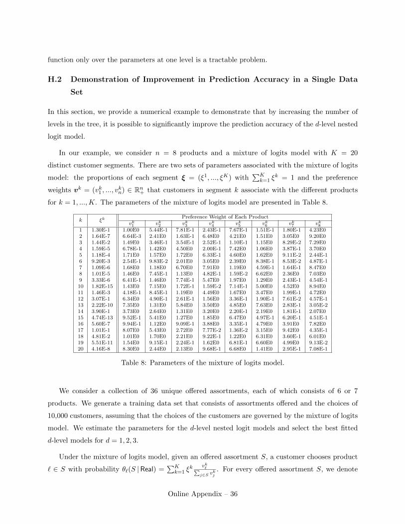
function only over the parameters at one level is a tractable problem.

H.2 Demonstration of Improvement in Prediction Accuracy in a Single Data

Set

In this section, we provide a numerical example to demonstrate that by increasing the number of

levels in the tree, it is possible to significantly improve the prediction accuracy of the d-level nested

logit model.

In our example, we consider n = 8 products and a mixture of logits model with K = 20

distinct customer segments. There are two sets of parameters associated with the mixture of logits

model: the proportions of each segment ξ = (ξ1, ..., ξK) with∑K

k=1 ξk = 1 and the preference

weights vk = (vk1 , ..., vkn) ∈ Rn+ that customers in segment k associate with the different products

for k = 1, ...,K. The parameters of the mixture of logits model are presented in Table 8.

k ξkPreference Weight of Each Product

vk1 vk2 vk3 vk4 vk5 vk6 vk7 vk81 1.30E-1 1.00E0 5.44E-1 7.81E-1 2.43E-1 7.67E-1 1.51E-1 1.80E-1 4.23E02 1.64E-7 6.64E-3 2.41E0 1.63E-1 6.48E0 4.21E0 1.51E0 3.05E0 9.20E03 1.44E-2 1.49E0 3.46E-1 3.54E-1 2.52E-1 1.10E-1 1.15E0 8.29E-2 7.29E04 1.59E-5 6.78E-1 1.42E0 4.50E0 2.00E-1 7.42E0 1.06E0 3.87E-1 3.70E05 1.18E-4 1.71E0 1.57E0 1.72E0 6.33E-1 4.60E0 1.62E0 9.11E-2 2.44E-16 9.20E-3 2.54E-1 9.83E-2 2.01E0 3.05E0 2.39E0 8.38E-1 8.53E-2 4.87E-17 1.09E-6 1.68E0 1.18E0 6.70E0 7.91E0 1.19E0 4.59E-1 1.64E-1 8.47E08 1.01E-5 1.46E0 7.45E-1 1.13E0 4.82E-1 1.59E-2 6.62E0 2.36E0 7.03E09 3.33E-6 6.41E-1 1.46E0 7.74E-1 5.47E0 1.97E0 1.29E0 2.43E-1 4.54E-110 1.82E-15 1.43E0 7.15E0 1.72E-1 1.59E-2 7.14E-1 5.00E0 4.52E0 8.94E011 1.46E-3 4.18E-1 8.45E-1 1.19E0 4.49E0 1.67E0 3.47E0 1.99E-1 4.72E012 3.07E-1 6.34E0 4.90E-1 2.61E-1 1.56E0 3.36E-1 1.90E-1 7.61E-2 4.57E-113 2.22E-10 7.35E0 1.31E0 5.84E0 3.50E0 4.85E0 7.63E0 2.83E-1 3.05E-214 3.90E-1 3.73E0 2.64E0 1.31E0 3.20E0 2.20E-1 2.19E0 1.81E-1 2.07E015 4.74E-13 9.52E-1 5.41E0 1.27E0 1.85E0 6.47E0 4.97E-1 6.20E-1 4.51E-116 5.60E-7 9.94E-1 1.12E0 9.09E-1 3.88E0 3.35E-1 4.79E0 3.91E0 7.82E017 1.01E-1 8.07E0 5.43E0 2.72E0 7.77E-2 1.36E-2 3.15E0 9.42E0 4.35E-118 4.81E-2 1.01E0 1.70E0 2.21E0 9.22E-1 1.22E0 6.31E0 3.60E-1 6.01E019 5.51E-11 1.54E0 9.15E-1 2.24E-1 1.62E0 6.81E-1 6.60E0 4.99E0 9.13E-220 4.16E-8 8.30E0 2.44E0 2.13E0 9.68E-1 6.68E0 1.41E0 2.95E-1 7.08E-1

Table 8: Parameters of the mixture of logits model.

We consider a collection of 36 unique offered assortments, each of which consists of 6 or 7

products. We generate a training data set that consists of assortments offered and the choices of

10,000 customers, assuming that the choices of the customers are governed by the mixture of logits

model. We estimate the parameters for the d-level nested logit models and select the best fitted

d-level models for d = 1, 2, 3.

Under the mixture of logits model, given an offered assortment S, a customer chooses product

` ∈ S with probability θ`(S |Real) =∑K

k=1 ξk vk`∑

j∈S vkj

. For every offered assortment S, we denote

Online Appendix – 36

the top-selling product under the mixture of logits model by

TopSell(S |Real) = arg max`∈Sθ`(S |Real) .

Moreover, for d = 1, 2, 3, we use θd` (S |Est) to denote the probability that a customer chooses

product ` ∈ S under the best fitted d-level nested logit model. We define the predicted top-selling

product under the d-level nested logit model as

TopSelld(S |Est) = arg max`∈Sθd` (S |Est) .

We are interested in comparing the predictive accuracy among the one, two and three-level nested

logit models. In particular, we want to evaluate the ability of the one, two and three-level nested

logit models to extrapolate and predict the top-selling products against the ground truth – the

mixture of logits model – over any arbitrary offered assortment. Note that we choose to compare

our fitted nested logit models directly against the ground truth instead of using validation and

testing data sets because in our generated training data, the ground truth, i.e., the parameters of

the underlying mixture of logits model, is already available.

We compare the predictive accuracy of the fitted models are follows. Note that the full

assortment of 8 products gives rise to 28−1 = 255 non-empty unique subsets of products. For each

subset of products S, we calculate TopSell(S |Real), the top-selling product under the mixture of

logits model and TopSelld (S |Est), the predicted top-selling product under each of the fitted d-level

nested logit models, for d = 1, 2, 3. Since there are 255 unique subsets of products, we have 255

choices of top-selling products for each of the mixture of logits model and the fitted one, two and

three-level nested logit models. The results for each d-level nested logit model can be summarized

in the form of a n × n confusion matrix. The confusion matrices for the one, two and three-level

nested logit models are shown in Figure 4.

For d = 1, 2, 3, in each confusion matrix for the d-level nested logit model, the rows correspond

to the actual top-selling products under the mixture of logits model; the columns correspond to

the predicted top-selling products under the fitted d-level nested logit model. For i = 1, ..., 8 and

j = 1, ..., 8, we denote each entry in the confusion matrix by

ConfMatrdi,j =∑

S⊆{1,...,8}

1l{TopSell(S |Real)=i,TopSelld(S |Est)=j} ,

where 1l{·} is the indicator function. Then, ConfMatrdi,j corresponds to the number of times that the

d-level nested logit model predicts the actual top-selling product i as j. Thus, the diagonal elements

Online Appendix – 37

in the confusion matrix show the number of correct predictions for each top-selling product. Any

non-zero off-diagonal element ConfMatrdi,j , i 6= j, is highlighted in bold, and it represents the number

of times that the d-level nested logit model falsely predicts the actual top-selling product i as j.

If all the off-diagonal entries in the confusion matrix are zero, then the d-level nested logit model

predicts with 100% accuracy.

We summarize the confusion matrix for each d-level nested logit model. The second last column

in each table that contains the confusion matrix for d-level model reports the total number of

predictions for each top-selling product under the mixture of logit models. The last column reports

the total number of false predictions under the fitted d-level nested logit model for each top-selling

product. Finally, the last row reports the total number of predictions for each top-selling product

under the fitted d-level nested logit model.

The results in Figure 4 show that the one-level nested logit model predicts 32 correctly out of

64 times, i.e., with 50% = 100% × 3264 accuracy when the actual top-selling product is product 4.

Similarly, the one-level nested logit model predicts with 50% = 100%× 12 accuracy when the actual

top-selling product is product 5. The two-level nested logit model performs much better than the

one-level, improving the predictive accuracy to 77% = 100% × 4964 and 100% = 100% × 64

64 when

the actual selling products are 4 and 5, respectively. The three-level nested logit model further

improves the predictive accuracy for top-selling product 4 to 100%. Overall, the one-level nested

logit model falsely predicts 35 out of 255 times; the two-level nested logit model falsely predicts

only 17 times; the three-level nested logit model significantly reduces the false predictions to just

2 times.

H.3 Numerical Experiments for an Ensemble of Data Sets

In the this section, we provide a numerical study to demonstrate that using larger number of levels

in the tree can help better predict the customer choice behavior. We generate data consisting of

the assortment offers and choices of multiple customers, under the assumption that the choices of

the customers are governed by a mixture of logits model. Using the generated data, we fit the

parameters of one, two and three-level nested logit models and compare the performance of the

fitted models in predicting the customer choice behavior.

Numerical Setup: Throughout our numerical study, the number of products is n = 8. Without

loss of generality, we can treat one of the products as the no-purchase option. We generate 50

data sets as the training data sets in our numerical study. To generate each data set, we use a

mixture of logits model with K = 20 customer segments. As explained before, the parameters of

Online Appendix – 38

Confusion Matrix for d = 1 No. of Pred. No. of

Actual Top- Predicted Top-Selling Product under Mix. of FalseSelling Product 1 2 3 4 5 6 7 8 Logits Model Pred.

1 128 0 0 0 0 0 0 0 128 02 0 16 0 0 0 0 0 1 17 1

3 0 0 4 0 0 1 0 0 5 14 0 0 0 32 0 0 0 32 64 32

5 0 0 0 0 1 0 1 0 2 1

6 0 0 0 0 0 7 0 0 7 07 0 0 0 0 0 0 1 0 1 0

8 0 0 0 0 0 0 0 31 31 0

No. of Pred. 128 16 4 32 1 8 2 64 255 35under Est. Model

Confusion Matrix for d = 2 No. of Pred. No. of

Actual Top- Predicted Top-Selling Product under Mix. of FalseSelling Product 1 2 3 4 5 6 7 8 Logits Model Pred.

1 128 0 0 0 0 0 0 0 128 02 0 16 0 0 0 0 0 1 17 13 0 0 4 0 0 1 0 0 5 14 0 0 0 49 0 0 0 15 64 15

5 0 0 0 0 2 0 0 0 2 06 0 0 0 0 0 7 0 0 7 07 0 0 0 0 0 0 1 0 1 0

8 0 0 0 0 0 0 0 31 31 0

No. of Pred. 128 16 4 49 2 8 1 47 255 17under Est. Model

Confusion Matrix for d = 3 No. of Pred. No. of

Actual Top- Predicted Top-Selling Product under Mix. of FalseSelling Product 1 2 3 4 5 6 7 8 Logits Model Pred.

1 128 0 0 0 0 0 0 0 128 02 0 16 0 0 0 0 0 1 17 13 0 0 4 0 0 1 0 0 5 1

4 0 0 0 64 0 0 0 0 64 05 0 0 0 0 2 0 0 0 2 0

6 0 0 0 0 0 7 0 0 7 07 0 0 0 0 0 0 1 0 1 08 0 0 0 0 0 0 0 31 31 0

No. of Pred. 128 16 4 64 2 8 1 32 255 2under Est. Model

Figure 4: Confusion matrices for the best fitted one, two and three-level nested logit models.

the mixture of logits model are the proportions of each segment ξ = (ξ1, . . . , ξK) ∈ [0, 1]K with∑Kk=1 ξ

k = 1, and for each segment k = 1, . . . ,K, the preference weights vk = (vk1 , . . . , vkn) ∈ Rn+

that customers in segment k associate with the different products. Under the mixture of logits

model, if we offer the assortment S, then a customer chooses product ` ∈ S with probability

θ`(S |Real) =∑K

k=1 ξk vk`∑

j∈S vkj

.

For each data set, we randomly choose the parameters of the mixture of logits model as

follows. We generate ξ = (ξ1, . . . , ξK) from a K-dimensional Dirichlet distribution with parameters

(α, . . . , α), so that the expectation of ξk is equal to 1K for all k = 1, . . . ,K. The coefficient

Online Appendix – 39

of variation of ξk is equal to√

K−1Kα+1 , and we calibrate the parameter α so that the coefficient of

variation is equal to 2.5. To introduce heterogeneity among different customer segments, we use the

following strategy to generate preference weights (v1, . . . ,vK). For each product ` = 1, . . . , n, we

sample σ` from the uniform distribution over [0, 1]. If σ` is close to one, then product ` is a specialty

product and customers in different segments associate significantly different preference weights with

this product. On the other hand, if σ` is close to zero, then product ` is a staple product and

customers in different segments evaluate product ` similarly, associating similar preference weights

with this product. To generate preference weights with such characteristics, for each product ` and

segment k, we sample ϑk` from the uniform distribution over [0, 10] and let vk` = (1 − σ`)ϑk` with

probability 1/2 and vk` = (1 + σ`)ϑk` with probability 1/2. In this case, if σ` is close to zero, then

vk` takes a value close to ϑk` . If, however, σ` is close to one, then vk` either takes a value close to

zero or a value close to 2ϑk` . Therefore, the parameter σ` indeed captures how much the preference

weight of product ` differs among the different customer segments.

Once we choose the parameters of the mixture of logits model, we generate choices of 10, 000

customers, assuming that the choices of the customers are governed by this choice model. In

particular, for each one of the 10, 000 customers, we randomly sample an assortment of products

offered to this customer. We consider 36 unique offered assortments, each of which consists

either 6 or 7 out of the 8 products. Given that the customer is offered a particular assortment,

we sample the choice of the customer within this assortment by using the choice probabilities

{θ`(S |Real) : ` = 1, . . . , n, S ⊆ {1, . . . , n}}. The assortments offered to 10, 000 customers and the

products chosen by these customers out of the assortments form one data set.

Parameter Estimation and Model Selection: For each data set, we estimate the parameters

of the one, two and three-level nested logit models by minimizing the Akaike Information Criterion

(AIC) value. Introduced by Akaike (1974), the AIC value is defined as

AICd = 2(ndp − 2Ld),

where ndp denotes the number of parameters in the model, and Ld denotes the value of the log-

likelihood function in (14). The model with the minimum AIC value minimizes the expected

Kullback-Leibler distance between the model and the underlying mixture of logits model.

By our construction as elaborated in the following two paragraphs, in each data set, ndp is a

constant for fixed d. Therefore, minimizing the AIC value is equivalent to maximizing the log-

likelihood function, for the models with the same number of levels. To maximize the log-likelihood

function, we sequentially maximize over the parameters at each level of the tree and stop when no

Online Appendix – 40

further improvement in the value of the log-likelihood is possible. We use the convex optimization

software CVX to solve the optimization problems; see Grant and Boyd (2008, 2013).

Note that there can be many different tree structures to consider for the two and three-level

nested logit models, corresponding to different organizations of the products in the tree. We use

the following simple heuristic to obtain a good tree structure and report the results for the best

tree structure that we find. We only consider the tree structures in which the non-leaf nodes in the

same level have equal number of children nodes. In particular, for the two-level nested logit model,

we only consider the tree structures in which the root node has two children and each node in level

one has four children. When we consider such tree structures, there are(

84

)/2 = 35 distinct ways

of placing the products in the tree. We estimate the parameters of the two-level nested logit model

for each one of these 35 tree structures. We choose the model that yields the smallest AIC value

as the best two-level nested logit model.

For the three-level nested logit model, we only consider the tree structures where each non-leaf

node has two children. When we consider such tree structures, there are(8

4)2

((42)2

)2= 315 distinct

ways of placing the products in the tree. Since the number of possible three-level tree structures is

large, we use a simple heuristic to focus on a small number of tree structures. In particular, by using

the approach in the previous paragraph, we find the best two-level tree structure. Once we have the

best two-level tree structure, we only consider the three-level tree structures that are compatible

with the best two-level tree structure. In other words, we let a and b be the two nodes in the first

level of the best two-level tree structure. We use Na and Nb to denote the sets of products that

are included in the subtrees rooted at nodes a and b. In the three-level tree structures we consider,

the sets of products that are included in the subtrees rooted at the two nodes in the first level of

the tree are identical to Na and Nb. Considering only such three-level tree structures reduces the

number of possibilities to(4

2)2

(42)2 = 9. Once we restrict our attention to 9 possible three-level tree

structures, similar to the approach in the previous paragraph, we estimate the parameters of the

three-level nested logit model for each one of these 9 tree structures, and choose the model that

has the smallest AIC value as the best three-level nested logit model.

In each data set, we also compare the AIC values of the one, two and three-level nested logit

models. For the one, two and three-level models we consider, n1p = 8, n2

p = 10 and n3p = 14. We

find that in general, a nested logit model with a larger number of levels has lower AIC value than a

nested logit model with smaller number of levels. This means that the issue of overfitting is under

control, if we use AIC to estimate the parameters.

Summary of Results: For each data set, we create three confusion matrices for the chosen one,

Online Appendix – 41

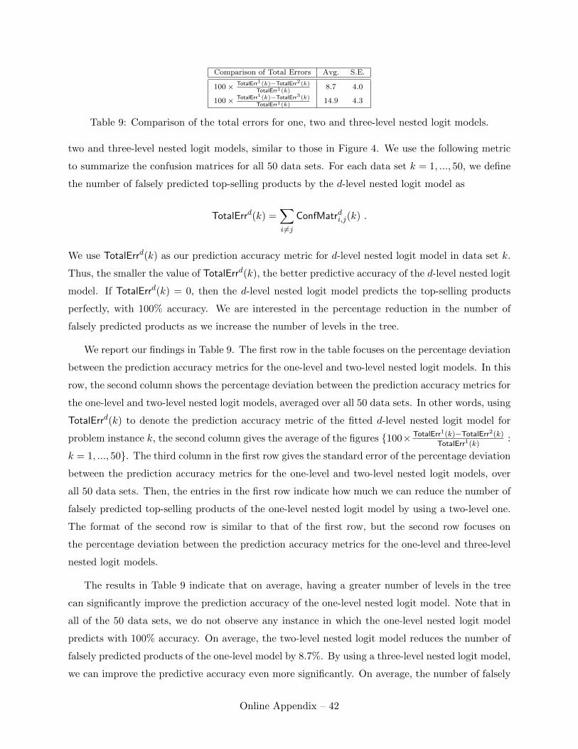
Comparison of Total Errors Avg. S.E.

100× TotalErr1(k)−TotalErr2(k)

TotalErr1(k)8.7 4.0

100× TotalErr1(k)−TotalErr3(k)

TotalErr1(k)14.9 4.3

Table 9: Comparison of the total errors for one, two and three-level nested logit models.

two and three-level nested logit models, similar to those in Figure 4. We use the following metric

to summarize the confusion matrices for all 50 data sets. For each data set k = 1, ..., 50, we define

the number of falsely predicted top-selling products by the d-level nested logit model as

TotalErrd(k) =∑i 6=j

ConfMatrdi,j(k) .

We use TotalErrd(k) as our prediction accuracy metric for d-level nested logit model in data set k.

Thus, the smaller the value of TotalErrd(k), the better predictive accuracy of the d-level nested logit

model. If TotalErrd(k) = 0, then the d-level nested logit model predicts the top-selling products

perfectly, with 100% accuracy. We are interested in the percentage reduction in the number of

falsely predicted products as we increase the number of levels in the tree.

We report our findings in Table 9. The first row in the table focuses on the percentage deviation

between the prediction accuracy metrics for the one-level and two-level nested logit models. In this

row, the second column shows the percentage deviation between the prediction accuracy metrics for

the one-level and two-level nested logit models, averaged over all 50 data sets. In other words, using

TotalErrd(k) to denote the prediction accuracy metric of the fitted d-level nested logit model for

problem instance k, the second column gives the average of the figures {100× TotalErr1(k)−TotalErr2(k)

TotalErr1(k):

k = 1, ..., 50}. The third column in the first row gives the standard error of the percentage deviation

between the prediction accuracy metrics for the one-level and two-level nested logit models, over

all 50 data sets. Then, the entries in the first row indicate how much we can reduce the number of

falsely predicted top-selling products of the one-level nested logit model by using a two-level one.

The format of the second row is similar to that of the first row, but the second row focuses on

the percentage deviation between the prediction accuracy metrics for the one-level and three-level

nested logit models.

The results in Table 9 indicate that on average, having a greater number of levels in the tree

can significantly improve the prediction accuracy of the one-level nested logit model. Note that in

all of the 50 data sets, we do not observe any instance in which the one-level nested logit model

predicts with 100% accuracy. On average, the two-level nested logit model reduces the number of

falsely predicted products of the one-level model by 8.7%. By using a three-level nested logit model,

we can improve the predictive accuracy even more significantly. On average, the number of falsely

Online Appendix – 42

predicted products is reduced by 14.9% when we use a three-level nested logit model. We note that

there are data sets in which the number of falsely predicted products of the lower-level nested logit

model is smaller than that of the higher-level nested logit model. Due to finite sample estimation

errors as we only estimated a limited number of two-level and three-level models, it is not possible

to guarantee that a higher-level nested logit model always improves the prediction accuracy of a

lower-level model, but our numerical study indicates that using a three-level nested logit model can

provide improvements in a great majority of the cases and the improvements can be significant.

H.4 Proof of Theorem H.1

In this section, we present the proof of Theorem H.1.

Proof: Using (8) and denoting Vj(St) by V t

j for simplicity, we write the log-likelihood function as

L (χ1, . . . ,χd−1,β)

=T∑t=1

log

(d∏

h=1

V tAn(ct,h)∑

j∈Sibling(An(ct,h)) Vtj

)

=

T∑t=1

log

eβct × d∏h=2

1(∑j∈Sibling(An(ct,h)) V

tj

)1−ηAn(ct,h−1)× 1∑

j∈Sibling(An(ct,1)) Vtj

=

T∑t=1

βct − d∑h=2

(1− ηAn(ct,h−1)

)log

∑j∈Children(An(ct,h−1))

V tj

− log

∑j∈Children(root)

V tj

=

T∑t=1

βct − d∑h=2

(1− ηAn(ct,h−1)

)log([V tAn(ct,h−1)

]1/ηAn(ct,h−1)

)− log

∑j∈Children(root)

V tj

,

where, letting Leaf and NonLeaf respectively be the leaf and non-leaf nodes in the tree, we use the

fact that

V tj =

0 if j ∈ Leaf and j /∈ St

eβj if j ∈ Leaf and j ∈ St(∑i∈Children(j) V

ti

)ηjif j ∈ NonLeaf .

In the expression above, the preference weight V tj for each node j depends on the parameters

(χ1, . . . ,χd−1,β), but we suppress this dependence for clarity. For each customer t and non-leaf

Online Appendix – 43

node j, let ytj be defined recursively as follows:

ytj =

log

( ∑`∈Children(j)∩St

eβ`

)if depth(j) = d− 1

log

( ∑i∈Children(j)

eηi·yti

)if depth(j) < d− 1 ,

where we set log 0 = −∞. Note that if none of the descendants of node j at the leaves belong to St,

then ytj = −∞ by our construction.

Claim 1: For each customer t and non-leaf node j, V tj = eηj ·y

tj .

We will prove the claim by induction on the depth of node j. If depth(j) = d− 1, then we have

that V tj =

(∑`∈Children(j)∩St e

β`)ηj

= eηj ·ytj , where the last equality follows from the definition of

ytj . Suppose the result is true for all nodes at depth h+ 1. Consider an arbitrary node j at depth

h < d− 1. By induction hypothesis, V tj =

(∑`∈Children(j) V

t`

)ηj=(∑

`∈Children(j) eη`·yt`

)ηj= eηj ·y

tj ,

where the last equality follows from the definition of ytj . This establishes the claim.

Using the claim above, the log-likelihood function is given by

L (χ1, . . . ,χd−1,β) =T∑t=1

βct − d∑h=2

(1− ηAn(ct,h−1)

)ytAn(ct,h−1) − log

∑j∈Children(root)

eηj ·ytj

=

T∑t=1

[βct −

d−1∑h=1

(1− ηAn(ct,h)

)ytAn(ct,h) − y

troot

]

=

T∑t=1

[βct −

d−1∑h=0

(1− ηAn(ct,h)

)ytAn(ct,h)

]

=

n∑`=1

M` β` −d−1∑h=0

∑j : depth(j)=h

(1− ηj)∑

t : St∩Descendant(j)6=∅

ytj , (15)

where M` is the total sales for product ` and Descendant(j) denotes all nodes that are descendants

of j, excluding j itself. Note that ytj is a function of χ1, . . . ,χd−1,β, so we will now write

ytj(χ1, . . . ,χd−1,β) to emphasize this dependence. Since ηj ∈ (0, 1] for all j ∈ NonLeaf and noting

the expression above, the following claim establishes the first part of the theorem.

Claim 2: For fixed χ1, . . . ,χd−1, for all t and j, ytj(χ1, . . . ,χd−1,β) is convex in β.

We will prove the claim by induction on the depth of node j. The result is true when depth(j) =

d−1 by the convexity of the log-sum-exp function; see Boyd and Vandenberghe (2004). Suppose the

result is true for all nodes of depth h+1. Consider node j at level h. It is a well-known results that if

Online Appendix – 44

the functions gi(·) are convex, then log(∑

i egi(·)) is also convex. Since ytj = log(

∑i∈Children(j) e

ηi·ytk),

we have that ytj(χ1, . . . ,χd−1,β) is also convex in β, completing the induction. This establishes

the claim. The following claim is useful to show the second part of the theorem.

Claim 3: For all t, h and j, ytj (χ1, . . . ,χh−1,χh,χh+1, . . . ,χd−1,β) is convex in χh.

Fix an arbitrary customer t and h ∈ {1, . . . , d − 1}. We show by induction on the node depth

that ytj is convex in χh for all nodes j. If Descendant(j)∩St = ∅, then ytj is constant at −∞, which is

convex. So, it suffices to consider only the nodes that are ancestors of products in St. First, consider

nodes j in levels d− 1, d− 2, . . . , h. By definition, ytj depends only on (ηi : i ∈ Descendant(j)). In

this case, the result automatically holds because ytj is independent of χh.

Now, consider node j such that depth(j) = h − 1. By definition, it holds that ytj =

log(∑

k∈Children(j) eηk·ytk

). For each k ∈ Children(j), depth(k) = h and ytk is independent of

χh, which implies that ytj depends on χh through (η` : ` ∈ Children(j)) via the log-sum-exp

function. Therefore, ytj is convex in χh.

Next, consider node j at level h− 2. Since ytj = log(∑

k∈Children(j) eηk·ytk

)and depth(k) = h− 1

for all k ∈ Children(j), ytj only depends on χh through ytk, which we have just shown to be convex

in χh. Therefore, ytj is also convex in χh. Exactly the same argument applies to all nodes in levels

h− 3, h− 4, . . . , 1 and this establishes the desired claim.

We will now use Claim 3 to establish the second part of the theorem. Note that χh appears in

the log-likelihood function in (15) in two terms

−∑

j:depth(j)=h

(1−ηj)

[ ∑t : St∩Descendant(j)6=∅

ytj

]and −

h−1∑g=1

∑j:depth(j)=g

(1−ηj)

[ ∑t : St∩Descendant(j)6=∅

ytj

].

The first term is an affine function in χh because for nodes j in level h,∑

t : St∩Descendant(j)6=∅ ytj

is independent of χh, so the first term is concave in χh. For the second term, χh only appears

through ykj , which we know from Claim 3 to be convex in χh, and thus, the second term is concave

in χh. Therefore, the log-likelihood function is concave in χh, as desired. 2

It is not difficult to generate counterexamples to show that the log-likelihood function is not

jointly concave in (χ1, . . . ,χd−1,β). Note that fixing β, the log-likelihood function in (15) contains

a product of (1− ηj) and ytj , which depends on (η` : ` ∈ Descendant(j)). Product of two variables

is not a jointly concave or convex function of the two variables. Thus, it is not difficult to see that

the log-likelihood function is not jointly concave in (χ1, . . . ,χd−1,β).

Online Appendix – 45

Online Appendix References

Akaike, H. 1974. A new look at the statistical model identification. IEEE Transactions on Automatic

Control 19 (6): 716–723.

Boyd, S., and L. Vandenberghe. 2004. Convex Optimization. Cambridge, UK: Cambridge University

Press.

Davis, J. M., G. Gallego, and H. Topaloglu. 2014. Assortment optimization under variants of the

nested logit model. Operations Research 62 (2): 250–273.

Grant, M., and S. Boyd. 2008. Graph implementations for nonsmooth convex programs. In Recent

Advances in Learning and Control, ed. V. Blondel, S. Boyd, and H. Kimura, Lecture Notes in

Control and Information Sciences, 95–110. Springer-Verlag Limited. http://stanford.edu/

~boyd/graph_dcp.html.

Grant, M., and S. Boyd. 2013, September. CVX: Matlab software for disciplined convex

programming, version 2.0 beta. http://cvxr.com/cvx.

Li, G., and P. Rusmevichientong. 2014. A greedy algorithm for the two-level nested logit model.

Operations Research Letters 42 (5): 319–324.

Talluri, K., and G. J. van Ryzin. 2004. Revenue management under a general discrete choice model

of consumer behavior. Management Science 50 (1): 15–33.

Train, K. 2003. Discrete Choice Methods with Simulation. New York, NY: Cambridge University

Press.

Online Appendix – 46