the cyclical component of us asset...

The cyclical component of US asset returns∗

David K. Backus,† Bryan R. Routledge,‡ and Stanley E. Zin§

(December 2008) April 6, 2010Preliminary (yes, still)

Abstract

We show that equity returns, the term spread, and excess returns on a broad range of assetsare positively correlated with future economic growth. The common tendency for excessreturns to lead the business cycle suggests a macroeconomic factor in the cyclical behaviorof asset returns and the equity premium in particular. We construct an exchange economythat illustrates how this might work. Its important ingredients are recursive preferences,stochastic volatility in consumption growth, and dynamic interaction between volatility andgrowth.

JEL Classification Codes: E32, E43, E44, G12.

Keywords: leading indicators, term spread, excess returns, business cycles, recursivepreferences, stochastic volatility.

∗ Thanks to Stijn Van Nieuwerburgh, Tom Tallarini, Amir Yaron for helpful comments. We also appreciatethe comments from seminar participants at University of Calgary, University of North Carolina at ChapelHill, University of Western Ontario, Wharton, and feedback from conference attendees at the NBER andSED meetings in Istanbul. The latest version of the paper is available at:http://pages.stern.nyu.edu/~dbackus/GE_asset_pricing/ms/BRZ_returns_latest.pdf.† Stern School of Business, New York University, and NBER; [email protected].‡ Tepper School of Business, Carnegie Mellon University; [email protected].§ Stern School of Business, New York University, and NBER; [email protected].

1 Introduction

We look at asset prices from the perspective of macroeconomists and ask: What do they tellus about the structure of the economy that generated them? We document two sets of factsthat we think are worth exploring further. The first is the well-known tendency for equityprices (or their growth rates) and term spreads (differences between long- and short-terminterest rates) to lead the business cycle. In US data, and to some extent in data for othercountries, fluctuations in these variables are positively correlated with economic growth upto 6 to 9 months in the future. Yet in virtually all business cycle models, everything —including equity prices and term spreads — moves up and down together. Indeed, thisis often treated as the defining feature of the business cycle, and therefore an attractiveproperty of a model. The second set of facts concerns excess returns. We show that excessreturns on a broad range of equity and bond portfolios also lead the cycle: high excessreturns are associated with high future growth. Moreover, they display similar cyclicalpatterns across a broad cross section. Portfolios with very different expected returns alldisplay a strikingly similar lead of the business cycle. This property is less widely knownand might even be new. It suggests that the cyclical component of excess returns is commonacross asset classes and has a macroeconomic origin.

If these are the facts, what do they tell us about the structure of the aggregate econ-omy? In a general markov environment, prices and quantities are functions of the stateof the economy. The facts suggest that asset prices reflect some feature of the state thatis correlated with future economic growth. We construct an example that shows how thismight work. To keep things simple, we consider a traditional exchange economy in whichthe only inputs are preferences and a stochastic process for consumption growth. The evi-dence points us to the consumption growth process. What we need, it seems, is a processin which predictable changes in future consumption growth show up now in equity pricesand term spreads. Preferences play a role, too, since they affect the value given to expectedfuture growth.

The evidence on excess returns poses more of a challenge. If we have constant variances(constant risk) in the consumption growth process and standard homothetic preferences(constant risk aversion), expected excess returns are constant, by construction. This pointis made by Atkeson and Kehoe (2008) and we think it’s a good one: you can’t talk sensiblyabout the cyclical behavior of excess returns without cyclical variation in risk and/or riskaversion. In order for excess returns to vary, we need variation in either aggregate aversionto risk or in risk itself. Both paths have been taken in the literature. Time variation in

aggregate risk aversion can have stem from risk preferences (e.g., generalized disappoint-ment aversion Routledge and Zin (2010)) or, perhaps, heterogeneity across agents (Guvenen(2009)). Alternatively, the level of risk can be time varying through, for example, stochas-tic volatility (Bansal and Yaron (2004)) or markov switching (Constantinides and Ghosh(2010)). Without making any claim to superiority, we consider changes in risk generatedby stochastic volatility in the consumption growth process. Crucially, recursive preferencesallow us to assign volatility a nonzero price. Cyclical variation requires, in addition, someinteraction between consumption growth (the cycle) and volatility (risk). The net result isa modest generalization of the environment of Bansal and Yaron (2004).

Here’s the plan. In Sections 2, we document the cyclical behavior financial variablesand economic growth. We do this with cross-correlation functions, which are useful visualrepresentations of the dynamic relations between variables. In Sections 3 we describe anexchange economy that has the elements in place to deliver something like the facts doc-umented earlier. Section 4 looks at some examples. The first strips down to a simplisticgrowth process that, hopefully, lets us see all the moving pieces of the model that contributeto the cross correlations. The second set of examples are numerical. There, we build onthe “long-run risk” component of Bansal and Yaron (2004) and deliver a calibration thatmatches the cross correlations that cross correlation patterns we see in the data. The lasttwo sections connect our work to the literature, clean up some loose ends, and point toissues that remain unresolved.

2 Financial indicators of business cycles

In the US and elsewhere, financial variables are commonly used as indicators of futureeconomic growth. Two of the most popular are equity prices (typically the growth rate orreturn of a broad-based index) and the term spread (the difference between a long-maturityinterest rate and a short rate). We describe the dynamic relations between these variablesand aggregate economic growth with cross-correlation functions. We then go on to look atexcess returns for a variety of assets with different cross-sectional properties.

Data

Our data cover the period from 1960 to the present. We use monthly series because thefiner time interval allows clearer identification of leads and lags than the quarterly data

2

commonly used in national income accounts and business cycle research. Definitions andsources are given in Appendix A, but here’s a summary. Most of our financial variablescome from CRSP and Ken French’s web site. Returns, rt, cover the whole month t; thereturn for October 2008, for example, refers to the period September 30 to October 31 andincludes any interim cash-flows (e.g., dividends). In addition to bond yields, we look at onemonth holding period returns on portfolios of bonds of a fixed maturity range (CRSP Famabond portfolios). Throughout, we calculate as the logarithms of gross returns because theyline up more neatly with our theory. Bond yields refer to the end of the month — the lasttrading day — so the yield associated with October 2008 is that for October 31.

Most of our macroeconomic variables come from FRED, the online data repository ofthe Federal Reserve Bank of St. Louis. They are typically time averages (e.g., a quantityper month). Industrial production for October 2008 is an estimate of the average for thatmonth. We also look at consumption and employment at similar frequencies. Aggregateprofit and dividend information is from Robert Shiller’s web site and represents monthlyearnings and dividends at S&P 500 companies. For all economic quantity data, Yt, wecompute growth rates as log-differences over the previous month yt = log Yt − log Yt−1, sothat the October growth rate is the growth rate of October over September.

To filter the data to focus on business cycles, we use centered year-on-year growth ratesyt = log Yt+6 − log Yt−6. This smoothes out the high-frequency variation in these serieswithout disturbing the timing. We use a similar filter with the financial data to calculatecentered annual returns rt = logPt+6 − logPt−6 where we construct Pt as the value of anindex from the monthly returns for the asset (i.e., average annual returns centered aroundmonth t). We think of year-on-year growth rates and returns as crude approximations tothe Hodrick-Prescott filter often used in business cycle analysis. We find the smoothedseries more informative about the cyclical component we are interested in. However, wepresent both the raw data and the smoothed data below.

The dynamic interrelations between financial indicators and economic growth are con-veniently summarized with cross-correlation functions. If r is a financial indicator and y isa measure of economic growth, their cross-correlation function is

ccf ry(k) = corr(rt, yt−k),

a function of the lag k. For negative values of k, this is the correlation of the financialindicator with future economic growth. If these correlations are nonzero, we say the financialindicator leads the business cycle. Similarly, positive values of k correspond to correlations

3

of the indicator with past economic growth; nonzero values suggest a lagging indicator. Ourinterest is in the former: financial variables that lead economic growth and thus serve as asource of information about the future.

Equity

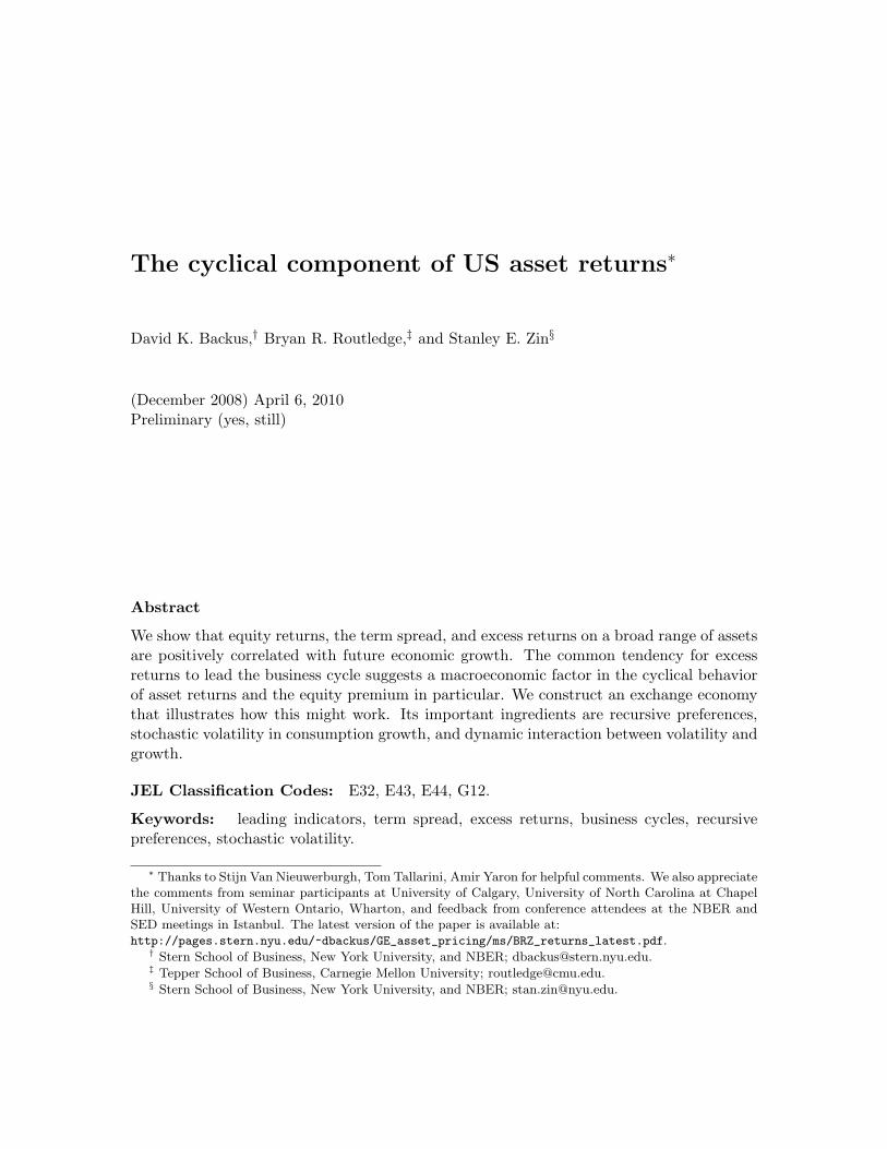
Consider equity returns. In Figure 2 we report the cross-correlation function for the (nom-inal) return on an aggregate portfolio of publicly-traded equity and the monthly growthrate of industrial production. Both series are inherently noisy — there’s little persistencein either series — yet we see a modest but clear pattern. The correlations on the left showthat equity returns are positively correlated with growth in industrial production up to oneyear in the future. The correlations are modest individually (the largest are between 0.12and 0.25) but exhibit a clear pattern. The correlations on the right are generally smaller.

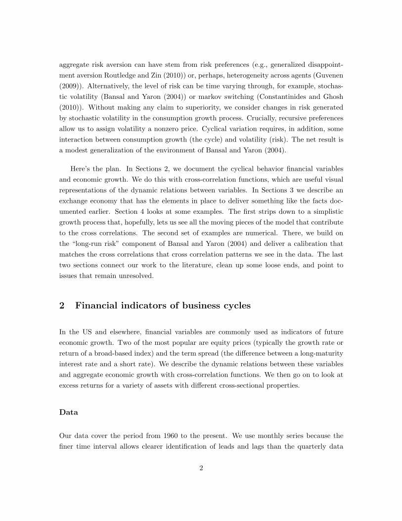
When we average growth over 12 months, the pattern emerges even more clearly: highequity returns are associated with high economic growth several months later. Figure 3ashows the correlation using year-on-year growth rates of industrial production with monthlyequity returns and Figure 3b shows the cross correlations of year-on-year growth with year-on-year returns. This is a typical result: correlations are larger and smoother if we useyear-on-year growth rates. These annualized series are closer to what is done in businesscycle research.

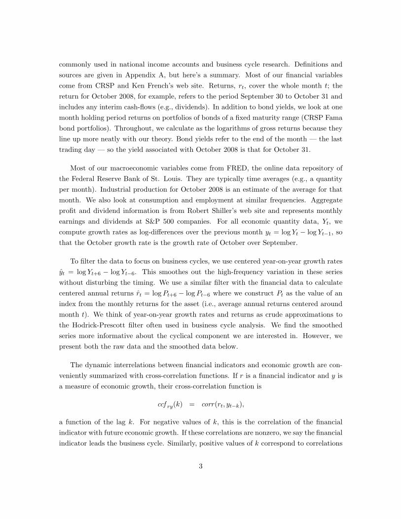
We use industrial production industrial production as our measure of economic activitysince it focusses focusses on easily measured quantities in industries like manufacturing,mining, and electric and gas utilities. These are the industries, along with construction,where the bulk of business cycle variation occurs.1 However, the key feature of the data –equity returns lead the business cycle – is robust to changes in our measurement of economicgrowth. Figure 4 replaces industrial production with employment (nonfarm employmentfrom the establishment survey) or consumption (total, per capita, real) and little changes.Similarly, we can measure economic activity with measures of corporate profits (S&P 500earnings and dividend growth) with similar results. The employment figures are a bitsharper and consumption less so. The corporate profit measures are sharper still. Whetherthese differences reflects better measurement or something else is hard to say.

Equity returns leading the business cycle is also robust to a number of variations inmeasurement and methodology. For example, we can use nominal or real returns with little

1See: http://www.federalreserve.gov/releases/G17/About.htm.

4

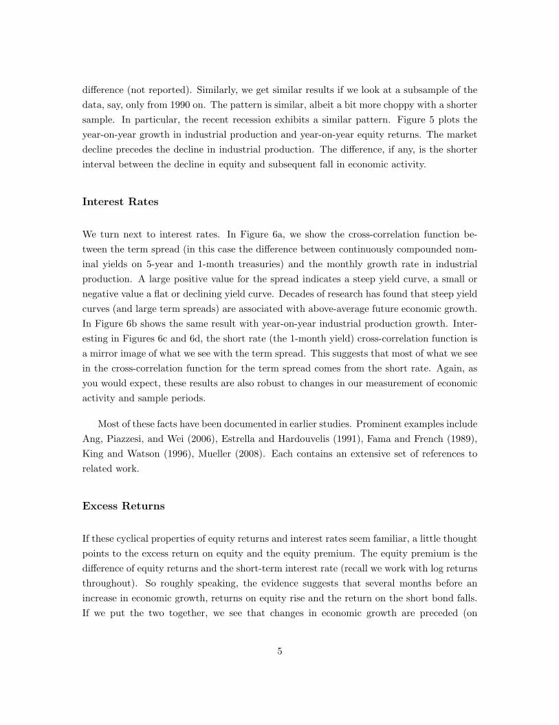
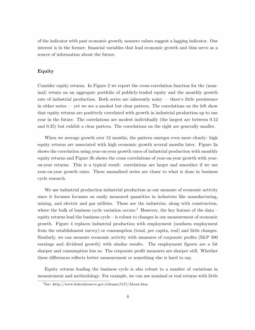
difference (not reported). Similarly, we get similar results if we look at a subsample of thedata, say, only from 1990 on. The pattern is similar, albeit a bit more choppy with a shortersample. In particular, the recent recession exhibits a similar pattern. Figure 5 plots theyear-on-year growth in industrial production and year-on-year equity returns. The marketdecline precedes the decline in industrial production. The difference, if any, is the shorterinterval between the decline in equity and subsequent fall in economic activity.

Interest Rates

We turn next to interest rates. In Figure 6a, we show the cross-correlation function be-tween the term spread (in this case the difference between continuously compounded nom-inal yields on 5-year and 1-month treasuries) and the monthly growth rate in industrialproduction. A large positive value for the spread indicates a steep yield curve, a small ornegative value a flat or declining yield curve. Decades of research has found that steep yieldcurves (and large term spreads) are associated with above-average future economic growth.In Figure 6b shows the same result with year-on-year industrial production growth. Inter-esting in Figures 6c and 6d, the short rate (the 1-month yield) cross-correlation function isa mirror image of what we see with the term spread. This suggests that most of what we seein the cross-correlation function for the term spread comes from the short rate. Again, asyou would expect, these results are also robust to changes in our measurement of economicactivity and sample periods.

Most of these facts have been documented in earlier studies. Prominent examples includeAng, Piazzesi, and Wei (2006), Estrella and Hardouvelis (1991), Fama and French (1989),King and Watson (1996), Mueller (2008). Each contains an extensive set of references torelated work.

Excess Returns

If these cyclical properties of equity returns and interest rates seem familiar, a little thoughtpoints to the excess return on equity and the equity premium. The equity premium is thedifference of equity returns and the short-term interest rate (recall we work with log returnsthroughout). So roughly speaking, the evidence suggests that several months before anincrease in economic growth, returns on equity rise and the return on the short bond falls.If we put the two together, we see that changes in economic growth are preceded (on

5

average) by a increase in the expected excess return on equity; that is an increase in theequity premium.

We see precisely this cyclical variation in excess returns in Figure 7. The figure shows thecross-correlation function for the excess return on equity and the growth rate of industrialproduction (both monthly and year-on-year are shown). The correlations for excess returnsare slightly larger than those for returns, but the pattern is similar. Evidently, most of thevariation in excess returns comes from the return rather than the short rate.

There is, of course, much variety in the excess returns across assets. Surprisingly, atleast to us, is that the same cyclical pattern appears in a wide range of equity portfolios.The basic theme is repeated in portfolios based on industry, portfolios based on firm marketcapitalization (“size”), and portfolios based on accounting measures (“book-to-market”).

Consider industry portfolios. Cross correlations for four examples are pictured in FigureFigure 8. We report two industries we thought would have highly cyclical production andsales (automobiles and machinery) and two that would be less cyclical (food and drugs).Their cross-correlation functions are nevertheless quite similar. Indeed, we could say thesame for virtually all 49 industry portfolios (based on SIC codes; not reported). At least toa first approximation, the cyclical behavior of these excess returns is the same.

The same is true of Fama-French (1992) portfolios. Four examples are given in Figure9: the smallest and largest firms ranked by market market capitalization and the lowestand highest ranked by book-to-market ratio (accounting measured book value divided bymarket capitalization). All four have positive correlations of excess returns with growth3-12 months in the future. Also striking (not reported) is that “difference portfolios” (theinfamous “small minus big” or SMB and “high minus low” or HML) show little cyclicalpattern: the cyclical behavior apparently cancels when you subtract one return from theother.

We find the common cyclical pattern in these portfolios surprising, because we know —from Fama and French (1992) and many others — that these portfolios have very differentreturn characteristics. Their average returns, in particular, are wildly different and the dif-ference portfolios are the standard factors used to fit the cross-section. The cross correlationfunctions suggest, however, that whatever these differences are, they are unrelated to thebusiness cycle.

If equity portfolios exhibit similar cyclical behavior, what about bonds? Bond returnsare noisier than the yields we looked at in the in Figure 6, but they display a clear cyclical

6

pattern. The four panels of Figure 10 are based on one-month returns on portfolios of UStreasuries with different maturities: 1-6 months, 19-24 months, 55-60 months, and 55-60months, and 115-120 months. Curiously, their cyclical behavior is similar (the year-on-yeargrowth and returns is plotted). This is, again, despite substantial differences in volatilityand average returns across the bond portfolios. This pattern is similar to that of equities,but not identical: where equities have a contemporaneous correlation close to zero withcurrent economic growth, bond returns have a noticeably negative correlation with growth0-5 months in the future.

Figures 11 and 12 look at the cyclical behavior of commodity excess returns (longpositions on a fully-collateralized futures contract). Oil, in Figure 11, mirrors the behaviorbonds. Low excess returns in oil precede growth and there is a positive contemporaneouscorrelation. Figure 12 looks at other commodities. There is little cyclical behavior seenin the agricultural commodities of wheat and oil. Copper leads the cycle and also showscontemporaneous correlation. (Casassus, Liu and Tang (2010) take a different look at thecorrelation structure in commodity prices.)

So what do we make of all this? We have seen that excess returns on a variety of equityand bond portfolios lead the business cycle: they are positively correlated with futureeconomic growth. Cyclical variation in excess returns suggests that risk premiums varysystematically over the business cycle. The common pattern across assets suggests that asingle macroeconomic factor might be able to account for all of them.

3 A theoretical exchange economy

The rest of the paper is concerned with mimicking the observed cyclical behavior of excessreturns in a theoretical environment. Before diving into the mechanics, it’s worth thinkinga little about what we need. Consider a stationary markov environment in which quantities(consumption, for example) and asset prices (equity and bonds) at any date t are functionsof a finite state vector st. Returns and excess returns between dates t and t + 1 are thenfunctions of successive states, say r(st, st+1). Variation in each of these variables thus reflectsvariation in the underlying state vector. The evidence of the last two sections indicates thatsome of this variation is positively correlated with future economic growth.

We illustrate this in a simple macroeconomic setting: an exchange economy with a rep-resentative agent. As usual in this sort of model, we specify preferences of a representative

7

agent and the stationary markov growth dynamics for the endowment that the agent con-sumes. Our version has a few key ingredients. First, our agent has recursive preferences.Second, the endowment process has predictable variation in both consumption growth andits conditional variance. Variation in the conditional mean is the “long run risk” compo-nent. Variation in the conditional variance (stochastic volatility) along with the recursivepreferences induce time variation in the equity premium. Finally, correlation with futureconsumption growth is produced directly, by specifying consumption growth as a processthat depends on past volatility. All of these features are necessary to account for the cycli-cal behavior of the excess returns, and in particular, the equity premium. The resultingmodel closely resembles the structure in Bansal and Yaron’s (2004). We think of it as aone-parameter extension. To make all the calculations we use a loglinear approximationmethod adapted from Hansen, Heaton, and Li (2008).

Environment

Preferences have the now-familiar recursive structure described by Kreps and Porteus(1978), Epstein and Zin (1989), and Weil (1989). If Ut is “utility from date t on,” preferencesfollow from the time aggregator V ,

Ut = V [ct, µt(Ut+1)] (1)

= [(1− β)cρt + βµt(Ut+1)ρ]1/ρ , (2)

and (expected utility) certainty equivalent function µ,

µt(Ut+1) =[Et(Uαt+1)

]1/α. (3)

The conventional interpretation is that ρ < 1 captures time preference (the intertemporalelasticity of substitution is 1/(1 − ρ)) and α < 1 captures risk aversion (the coefficient ofrelative risk aversion is 1− α). Additive utility is a special case with α = ρ.

Both the time aggregator and the certainty equivalent function are homogeneous ofdegree one, which allows us to scale everything by current consumption and convert ourproblem to one in growth rates. If we define scaled utility ut = Ut/ct, equation (2) can beexpressed

ut = [(1− β) + βµt(gt+1ut+1)ρ]1/ρ , (4)

where gt+1 = ct+1/ct is the growth rate of the endowment (consumption).

8

With these preferences, the pricing kernel (marginal rate of substitution) is

mt+1 = β(ct+1/ct)ρ−1 [Ut+1/µt(Ut+1)]α−ρ

= βgρ−1t+1 [gt+1ut+1/µt(gt+1ut+1)]α−ρ . (5)

See Appendix B. The pricing kernel is the heart of any asset pricing model, so (5) is centralto the properties of asset prices and returns. We can see the role of recursive preferences inthe pricing kernel. The first part of the kernel is risk-neutral discount factor, β, adjusted for“short-run risk” consumption growth risk (ct+1/ct)ρ−1 The next term, (Ut+1/µt(Ut+1))α−ρ.is like an innovation in future utility (note the presence of the certainty equivalent oper-ator rather than expectation operator). This term determines how predictable changes inconsumption growth and its volatility are priced. Note it drops out if preferences are timeadditive, α = ρ.

We specify a general linear process for the logarithm of consumption growth. Let statevariables xt (a vector of arbitrary dimension) and vt (volatility, a scalar) follow

xt+1 = Axt + a(vt − v) + v1/2t Bwt+1 (6)

vt+1 = (1− ϕv)v + ϕvvt + bwt+1, (7)

where v is the unconditional mean of vt, {wt} ∼ NID(0, I), and Bb> = 0 (innovations inxt and vt are uncorrelated).2 The aggregate state is therefore st = (xt, vt). Consumptiongrowth is tied to xt: log gt = g+ e>xt for some constant vector e. This gives us flexible dy-namics for xt, and therefore consumption growth. The conditional variance of consumptiongrowth is proportional to vt:

Vart (log gt+1) = e>BB>e vt.

This structure also allows some interaction between the dynamics of xt and vt through thevector a. If a = 0, consumption growth and volatility are uncorrelated. In the examplesthat follow we a will be a positive (and scalar). We’ll see later that all of these features— a predictable component in consumption growth, stochastic volatility, and interactionbetween the two — are needed to account for the cyclical behavior of asset returns.

Loglinear approximation of the pricing kernel

Asset prices in this setting are functions of the state variables and returns are functionsof prices. We derive loglinear approximations to equilibrium asset prices with the goal of

2Formally, wt is approximately normal since it is truncated to ensure vt ≥ 0.

9

having something that is both easy to compute and relatively transparent. We break thesolution process into steps to show how it works.

Step 1. Approximate time aggregator. The starting point is equation (4), which is notloglinear unless ρ = 0. A first-order approximation of log ut in logµt around the pointlogµt = logµ is

log ut = ρ−1 log [(1− β) + βµt(gt+1ut+1)ρ]

= ρ−1 log[(1− β) + βeρ logµt(gt+1ut+1)

]≈ κ0 + κ1 logµt(gt+1ut+1), (8)

where

κ1 = βeρ log µ/[(1− β) + βeρ log µ]

κ0 = ρ−1 log[(1− β) + βeρ log µ]− κ1 logµ.

The approximation is exact when ρ = 0, in which case κ0 = 0 and κ1 = β. See Hansen,Heaton, and Li (2008, Section III).

The rest of the solution follows those of many approximate solutions to dynamic pro-grams: we guess a value function of a specific form with unknown parameters, substituteoptimal decisions into the Bellman equation, and solve for the unknown parameters. Inthis case the decision is trivial (consume the endowment), but the rest of the solution isthe same. Equation (8) serves as the (approximate) Bellman equation with κ1 in the roleof discount factor.

Step 2. Guess value function. We conjecture an approximate scaled value function

log ut = u+ p>x xt + pvvt

with coefficients (u, px, pv) to be determined.

Step 3. Compute certainty equivalent. The novel ingredient of (8) is the certainty equivalentµt(gt+1ut+1). Note that

log(gt+1ut+1) = u+ g + (e+ px)>xt+1 + pvvt+1

= u+ g + (e+ px)>[Axt + a(vt − v) + v1/2t Bwt+1] + pv[(1− ϕv)v + ϕvvt + bwt+1].

The certainty equivalent is

logµt(gt+1ut+1) = u+ g − (e+ px)>av + (e+ px)>[Axt + a(vt − v)] + pv[(1− ϕv)v + ϕvvt]

+ (α/2)[(e+ px)>BB>(e+ px)vt + p2vbb>].

10

This follows from common properties of lognormal random variables: if an arbitrary randomvariable log x ∼ N(a, b), then logE(x) = a+ b/2 and logµ(x) = a+ αb/2.

Step 4. Solve Bellman equation. If we substitute the certainty equivalent into (4) and lineup coefficients, we have

u = κ0 + κ1

[u+ g + pv(1− ϕv)v + (α/2)p2

vbb>]

p>x = e>(κ1A)(I − κ1A)−1

pv = κ1(1− κ1ϕv)−1[(e+ px)>a+ (α/2)(e+ px)>BB>(e+ px)

].

The constant u plays no role in the pricing that follows. The coefficient px has the form

p>x = e>[(κ1A) + (κ1A)2 + (κ1A)3 + · · ·

].

We think of it as capturing the Bansal-Yaron effect. xt affects expected future consumptiongrowth. Utility (scaled) is the valuation of that future consumption with κ1 as the “discountfactor” (recall κ1 = β when ρ = 0.) For example, with white noise consumption growthwhere A = 0 in equation (6), then xt has zero effect on utility and px = 0. The pv

term determines how innovations to the conditional volatility change scaled utility. Theκ1/(1− κ1ϕv) again comes from discounting. The shock to volatility decays at rate ϕv andthe “discount rate” is κ1. The shock has two effects on utility. The first (the one involvingthe interaction parameter a) comes from the impact of volatility vt on future values of xtand expected future consumption growth. The second (the one involving α/2) summarizesthe impact of vt on the through volatility. The sign of this term is determined by the relativemagnitude of utility from growth and disutility from volatility. To calculate pv, note

(e+ px)> = e>(I − κ1A)−1.

The solution for pv follows immediately.

Step 5. Derive pricing kernel. With these inputs, we can calculate the pricing kernel. The(scaled) utility enters the pricing kernel through the term

log(gt+1ut+1)− logµt(gt+1ut+1) = −(α/2)[p2vbb> + (e+ px)>BB>(e+ px)vt

]+ v

1/2t (e+ px)>Bwt+1 + pvbwt+1.

The right-hand side has two kinds of terms: innovations (the terms with wt+1) and penaltiesfor risk (those with α/2). The pricing kernel (5) follows as

logmt+1 = log β + (ρ− 1) log gt+1 + (α− ρ) [log(gt+1ut+1)− logµt(gt+1ut+1)]

11

= log β + (ρ− 1)(g − e>av)− (α− ρ)(α/2)p2vbb>

+ (ρ− 1)e>Axt + [(ρ− 1)e>a− (α− ρ)(α/2)(e+ px)>BB>(e+ px)]vt

+ v1/2t [(ρ− 1)e+ (α− ρ)(e+ px)]>Bwt+1 + (α− ρ)pvbwt+1

= δ0 + δ>x xt + δvvt + v1/2t λ>xwt+1,+λ>v wt+1, (9)

with the implicit definitions of (δ0, δx, δv, λx, λv). You may recognize this as a close relativeof so-called affine models of bond pricing. The main difference is that the parameters arenot free: they’re tied to preferences and the consumption growth process.

The pricing kernel illustrates the interaction of recursive preferences, predictability ofconsumption growth, and stochastic volatility. The state variables xt play a role only tothe extent they help to forecast future consumption growth. If the state variables do notforecast growth (in other words, when A = 0), they do not appear in the pricing kernel(δx = 0). If the state variables xt do enter the pricing kernel, their impact is governedby the intertemporal substitution parameter ρ. Volatility vt appears here for two reasons.Volatility helps predict future consumption growth (via the a volatility-growth interactionterm). The impact of this is controlled by intertemporal substitution (ρ). The volatilityterm also enters directly because it controls the conditional variance (the second term inδv). The size of this effect depends on risk aversion (through α/2) and the departure fromadditive preferences (the difference α − ρ). When either is zero, the term is also zero, andvolatility affects the pricing kernel only through its impact on expected future consumptiongrowth.

In what sense is our solution an approximation? The only relation that isn’t exact is(8), which is exact when ρ = 0. Moreover, relative to standard methods (linearize aroundthe deterministic steady state), uncertainty plays a central role.

Asset returns

Given a pricing kernel m, (gross) asset returns r satisfy the pricing relation

Et (mt+1rt+1) = 1.

An asset, for our purposes, is a claim at date t to a dividend stream {dt+j} for j ≥ 1. Weuse the pricing kernel (9) to derive prices and returns for a number of common assets, whoseproperties can then be compared to those we documented in Sections 2. For bonds, we willlook at the short rate and multiperiod default-free bonds. For equity, we will look at a claim

12

to next periods endowment, a consumption strip, and a claim to the endowment at all futuredates, a consumption stream. We skip the pricing of more complicated securities, like aclaim to a levered dividend stream that is imperfectly correlated with consumption growth.Solving for the returns on this sort of security would involve an additional approximation.For now, we will stick to securities whose returns we can solve exactly. (Despite the log-linear structure, not all these expressions that follow are transparent. The example thatfollows in Section 4.1 solves an example with a single state variable.)

Short rate. The dividend on a short-term default-free security is one unit of the consumptiongood next period: dt+1 = 1. The price of this 1-period (real) bond is q1t = Etmt+1 and thereturn is r1t+1 = 1/q1t = 1/Etmt+1. Thus

log r1t+1 = − log q1t = −(δ0 + λ>v λv/2)− δ>x xt − (δv + λ>x λx/2)vt,

The short rate, as you would expect, is a loglinear function of the state (xt, vt). This isnot obvious from the expression, but in the examples we look at below, we’ll see that thedynamics of the short rate are dominated by the volatility term (a similar flavor as Atkeson-Kehoe (2008)). In addition, we use the familiar preference calibration where α and α − ρare negative, the short rate is decreasing in volatility. The example in Section 4.1 illustratesthis better.

Consumption Strip. A consumption “strip” pays the consumption at (the single) date t+s;dt+s = ct+s. This isn’t a real asset, but it illustrates how the various ingredients interact.Let’s focus on the one-period ahead strip for now. Define qst as the price-dividend ratio forstrip with maturity s at date t. For s = 1,

qst = Et (mt+1gt+1)

and the return is rst+1 = gt+1/qst . The log growth rate is

log gt+1 = g + e>xt+1 = g + e>[Axt + a(vt − v) + v1/2t Bwt+1].

The price is

log qst = (δ0 + g − e>av + λ>v λv/2) + (δ>x + e>A)xt + [δv + e>a+ (λ>x + e>B)(λx +B>e)/2]vt

and the return is

log rst+1 = −(δ0 + λ>v λv/2)− δ>x xt − [δv + (λ>x + e>B)(λx +B>e)/2]vt + v1/2t e>Bwt+1.

The excess return is therefore

log rst+1 − log r1t+1 = (1/2)[λ>x λx − (λ>x + e>B)(λx +B>e)]vt + v1/2t e>Bwt+1.

13

This expression gives us a look at how the cross correlation function for excess returnswith consumption growth might work. Note the excess return here does not depend onthe predictable component of consumption growth. Neither xt state nor the volatility-growth interaction term, a, appear. The predictable component has an identical effecton all returns; hence it does not show up in excess returns. This is a general result thatcomes from the afine pricing kernel. This suggests the cross correlation function of excessreturns with consumption growth will largely reflect cross correlation function of volatilitywith consumption growth (we re-visit this with the example in Section 4.1). Second, notethat innovations to volatility (the bwt+1 term) does not show up in excess returns of theconsumption strip since we are looking at a single period security (vt+1 does not affect gt+1).

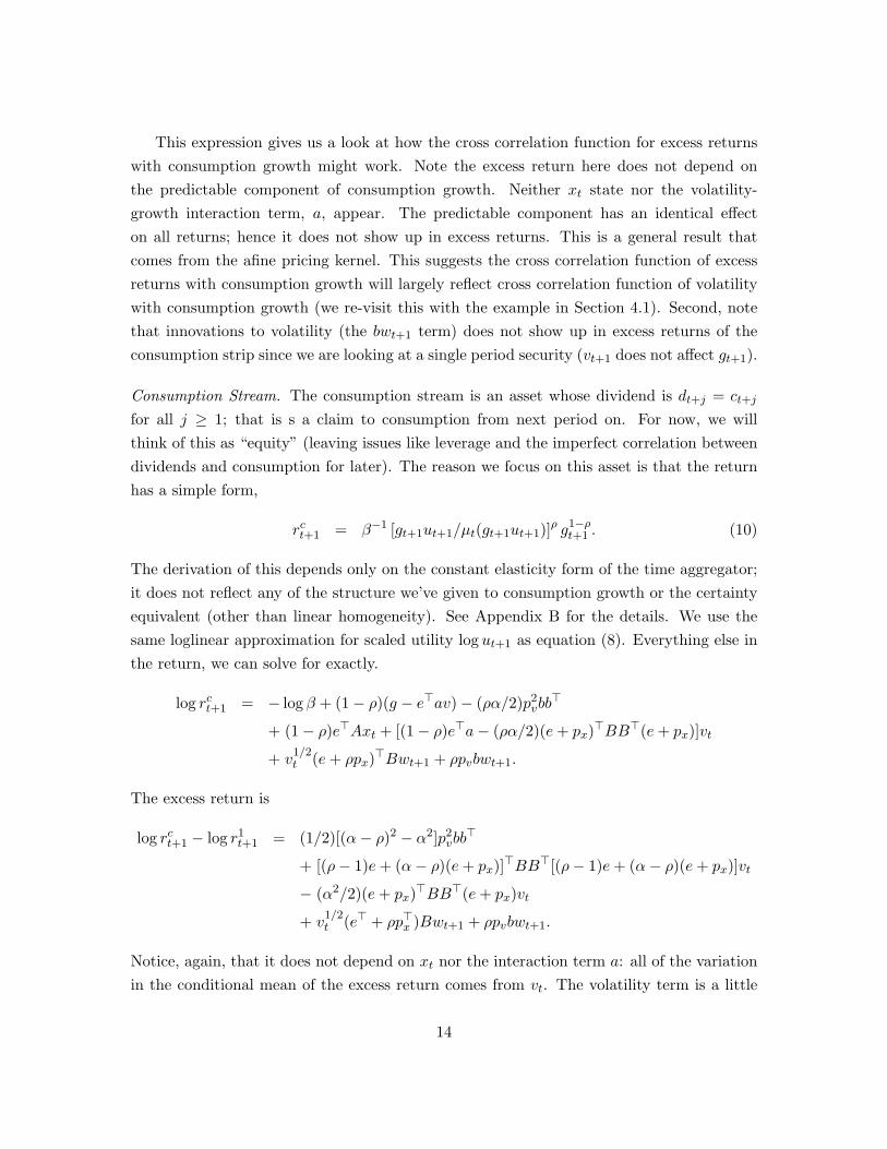
Consumption Stream. The consumption stream is an asset whose dividend is dt+j = ct+j

for all j ≥ 1; that is s a claim to consumption from next period on. For now, we willthink of this as “equity” (leaving issues like leverage and the imperfect correlation betweendividends and consumption for later). The reason we focus on this asset is that the returnhas a simple form,

rct+1 = β−1 [gt+1ut+1/µt(gt+1ut+1)]ρ g1−ρt+1 . (10)

The derivation of this depends only on the constant elasticity form of the time aggregator;it does not reflect any of the structure we’ve given to consumption growth or the certaintyequivalent (other than linear homogeneity). See Appendix B for the details. We use thesame loglinear approximation for scaled utility log ut+1 as equation (8). Everything else inthe return, we can solve for exactly.

log rct+1 = − log β + (1− ρ)(g − e>av)− (ρα/2)p2vbb>

+ (1− ρ)e>Axt + [(1− ρ)e>a− (ρα/2)(e+ px)>BB>(e+ px)]vt

+ v1/2t (e+ ρpx)>Bwt+1 + ρpvbwt+1.

The excess return is

log rct+1 − log r1t+1 = (1/2)[(α− ρ)2 − α2]p2vbb>

+ [(ρ− 1)e+ (α− ρ)(e+ px)]>BB>[(ρ− 1)e+ (α− ρ)(e+ px)]vt

− (α2/2)(e+ px)>BB>(e+ px)vt

+ v1/2t (e> + ρp>x )Bwt+1 + ρpvbwt+1.

Notice, again, that it does not depend on xt nor the interaction term a: all of the variationin the conditional mean of the excess return comes from vt. The volatility term is a little

14

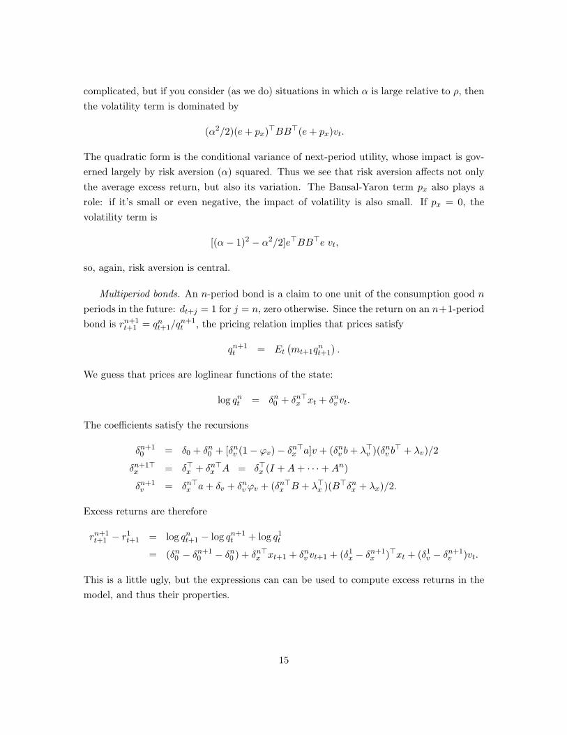
complicated, but if you consider (as we do) situations in which α is large relative to ρ, thenthe volatility term is dominated by

(α2/2)(e+ px)>BB>(e+ px)vt.

The quadratic form is the conditional variance of next-period utility, whose impact is gov-erned largely by risk aversion (α) squared. Thus we see that risk aversion affects not onlythe average excess return, but also its variation. The Bansal-Yaron term px also plays arole: if it’s small or even negative, the impact of volatility is also small. If px = 0, thevolatility term is

[(α− 1)2 − α2/2]e>BB>e vt,

so, again, risk aversion is central.

Multiperiod bonds. An n-period bond is a claim to one unit of the consumption good nperiods in the future: dt+j = 1 for j = n, zero otherwise. Since the return on an n+1-periodbond is rn+1

t+1 = qnt+1/qn+1t , the pricing relation implies that prices satisfy

qn+1t = Et

(mt+1q

nt+1

).

We guess that prices are loglinear functions of the state:

log qnt = δn0 + δn>x xt + δnv vt.

The coefficients satisfy the recursions

δn+10 = δ0 + δn0 + [δnv (1− ϕv)− δn>x a]v + (δnv b+ λ>v )(δnv b

> + λv)/2

δn+1>x = δ>x + δn>x A = δ>x (I +A+ · · ·+An)

δn+1v = δn>x a+ δv + δnvϕv + (δn>x B + λ>x )(B>δnx + λx)/2.

Excess returns are therefore

rn+1t+1 − r

1t+1 = log qnt+1 − log qn+1

t + log q1t= (δn0 − δn+1

0 − δn0 ) + δn>x xt+1 + δnv vt+1 + (δ1x − δn+1x )>xt + (δ1v − δn+1

v )vt.

This is a little ugly, but the expressions can can be used to compute excess returns in themodel, and thus their properties.

15

4 Examples – Cyclical behavior of theoretical excess returns

We find a couple of examples helpful to sort out how the preferences and the process forendowment growth lead to the cross correlation patterns we see in the data. The firstexample begins with a simpler process. The second example uses an endowment processthat builds from Bansal and Yaron (2004) and generates asset return features we see in thedata.

4.1 Stochastic volatility and no long-run risk

Here is a simpler scalar process for endowment growth where the algebra is a bit moretransparent. Define consumption growth as gt+1 = ct+1/ct with dynamics

log gt+1 = g + a(vt − v) + v1/2t εt+1 (11)

vt+1 = (1− ϕv)v + ϕvvt + σηt+1 (12)

where v is the unconditional mean of vt, g is the unconditional mean of gt and 0 < ϕv < 1is the autocorrelation of vt. The εt, ηt ∼ NID(0, 1) and uncorrelated. This specificationhas predictable variation in the conditional variance (stochastic volatility). The conditionalmean of consumption growth is correlated with the volatility through the (scalar) parametera (our numerical illustration has a ≥ 0). The only state variable, st, here is the conditionalvolatility vt. The conditional mean of endowment growth has simple AR(1) dynamics andis too simple to generate realistic asset prices. It is missing the “long-run risk” component(since we have set A = 0 in equation (6)). However, it does illustrate how preferences andendowment link to the cross-correlation functions.

We can solve this example with exactly the same steps as in the previous section or justplug A = 0 into the previous solutions (or, of course, do both just to be inefficient). To getstarted, the pricing kernel is

logmt+1 = δ0 + δvvt + λxv1/2t εt+1 + λvσηt+1

with

δo = log β + (ρ− 1)(g − av)− (α− ρ)(α/2)p2vσ

2

δv = (ρ− 1)a− (α− ρ)(α/2)

λx = α− 1

λv = (α− ρ)pvσ

pv = κ1(1− κ1ϕv)−1(a+ α/2)

16

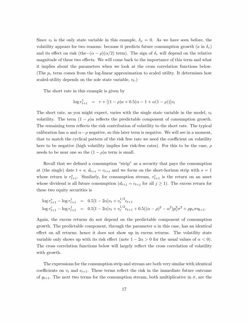
Since vt is the only state variable in this example, δx = 0. As we have seen before, thevolatility appears for two reasons: because it predicts future consumption growth (a in δv)and its effect on risk (the−(α − ρ)(α/2) term). The sign of δv will depend on the relativemagnitude of these two effects. We will come back to the importance of this term and whatit implies about the parameters when we look at the cross correlation functions below.(The pv term comes from the log-linear approximation to scaled utility. It determines howscaled-utility depends on the sole state variable, vt.)

The short rate in this example is given by

log r1t+1 = r + [(1− ρ)a+ 0.5(α− 1 + α(1− ρ))]vt

The short rate, as you might expect, varies with the single state variable in the model, vtvolatility. The term (1 − ρ)a reflects the predictable component of consumption growth.The remaining term reflects the risk contribution of volatility to the short rate. The typicalcalibration has α and α−ρ negative, so this later term is negative. We will see in a moment,that to match the cyclical pattern of the risk free rate we need the coefficient on volatilityhere to be negative (high volatility implies low risk-free rates). For this to be the case, ρneeds to be near one so the (1− ρ)a term is small.

Recall that we defined a consumption “strip” as a security that pays the consumptionat (the single) date t + s; dt+s = ct+s and we focus on the short-horizon strip with s = 1whose return is rst+1. Similarly, for consumption stream, rct+1 is the return on an assetwhose dividend is all future consumption (dt+j = ct+j for all j ≥ 1). The excess return forthese two equity securities is

log rst+1 − log r1t+1 = 0.5[1− 2α]vt + v1/2t εt+1

log rct+1 − log r1t+1 = 0.5[1− 2α]vt + v1/2t εt+1 + 0.5((α− ρ)2 − α2)p2

vσ2 + ρpvσηt+1.

Again, the excess returns do not depend on the predictable component of consumptiongrowth. The predictable component, through the parameter a in this case, has an identicaleffect on all returns; hence it does not show up in excess returns. The volatility statevariable only shows up with its risk effect (note 1− 2α > 0 for the usual values of α < 0).The cross correlation functions below will largely reflect the cross correlation of volatilitywith growth.

The expressions for the consumption strip and stream are both very similar with identicalcoefficients on vt and εt+1. These terms reflect the risk in the immediate future outcomeof gt+1. The next two terms for the consumption stream, both multiplicative in σ, are the

17

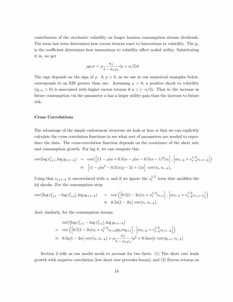
contribution of the stochastic volatility on longer horizon consumption stream dividends.The term last term determines how excess returns react to innovations to volatility. The pvis the coefficient determines how innovations to volatility affect scaled utility. Substitutingit in, we get

ρpvσ = ρκ1

1− κ1ϕv(a+ α/2)σ

The sign depends on the sign of ρ. A ρ > 0, as we use in our numerical examples below,corresponds to an EIS greater than one. Assuming ρ > 0, a positive shock to volatility(ηt+1 > 0) is associated with higher excess returns if a > (−α/2). That is; the increase infuture consumption via the parameter a has a larger utility gain than the increase to futurerisk.

Cross Correlations

The advantage of the simple endowment structure we look at here is that we can explicitlycalculate the cross correlation functions to see what sort of parameters are needed to repro-duce the data. The cross-correlation function depends on the covariance of the short rateand consumption growth. For lag k, we can compute this

cov(log r1t+1, log gt+1−k) = cov([[(1− ρ)a+ 0.5(α− ρ)α− 0.5(α− 1)2]vt

],[avt−k + v

1/2t−kεt+1−k

])

≈[(1− ρ)a2 − 0.5(α(ρ− 2) + 1)a

]cov(vt, vt−k),

Using that εt+1−k is uncorrelated with vt and if we ignore the v1/2t term that modifies the

iid shocks. For the consumption strip

cov([log rst+1 − log r1t+1], log gt+1−k) = cov([

0.5[1− 2α]vt + v1/2t εt+1

],[avt−k + v

1/2t−kεt+1−k

])≈ 0.5a[1− 2α] cov(vt, vt−k).

And, similarly, for the consumption stream

cov([log rct+1 − log r1t+1], log gt+1−k)

= cov([

0.5[1− 2α]vt + v1/2t εt+1ρpvσηt+1

],[avt−k + v

1/2t−kεt+1−k

])≈ 0.5a[1− 2α] cov(vt, vt−k) + ρ

κ1

1− κ1ϕv[a2 + 0.5aα]σ cov(ηt+1, vt−k)

Section 2 tells us our model needs to account for two facts: (1) The short rate leadsgrowth with negative correlation (low short rate precedes boom); and (2) Excess returns on

18

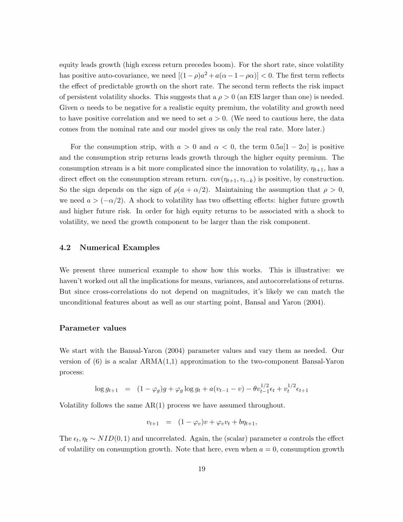
equity leads growth (high excess return precedes boom). For the short rate, since volatilityhas positive auto-covariance, we need [(1−ρ)a2 +a(α−1−ρα)] < 0. The first term reflectsthe effect of predictable growth on the short rate. The second term reflects the risk impactof persistent volatility shocks. This suggests that a ρ > 0 (an EIS larger than one) is needed.Given α needs to be negative for a realistic equity premium, the volatility and growth needto have positive correlation and we need to set a > 0. (We need to cautious here, the datacomes from the nominal rate and our model gives us only the real rate. More later.)

For the consumption strip, with a > 0 and α < 0, the term 0.5a[1 − 2α] is positiveand the consumption strip returns leads growth through the higher equity premium. Theconsumption stream is a bit more complicated since the innovation to volatility, ηt+1, has adirect effect on the consumption stream return. cov(ηt+1, vt−k) is positive, by construction.So the sign depends on the sign of ρ(a + α/2). Maintaining the assumption that ρ > 0,we need a > (−α/2). A shock to volatility has two offsetting effects: higher future growthand higher future risk. In order for high equity returns to be associated with a shock tovolatility, we need the growth component to be larger than the risk component.

4.2 Numerical Examples

We present three numerical example to show how this works. This is illustrative: wehaven’t worked out all the implications for means, variances, and autocorrelations of returns.But since cross-correlations do not depend on magnitudes, it’s likely we can match theunconditional features about as well as our starting point, Bansal and Yaron (2004).

Parameter values

We start with the Bansal-Yaron (2004) parameter values and vary them as needed. Ourversion of (6) is a scalar ARMA(1,1) approximation to the two-component Bansal-Yaronprocess:

log gt+1 = (1− ϕg)g + ϕg log gt + a(vt−1 − v)− θv1/2t−1εt + v

1/2t εt+1

Volatility follows the same AR(1) process we have assumed throughout.

vt+1 = (1− ϕv)v + ϕvvt + bηt+1,

The εt, ηt ∼ NID(0, 1) and uncorrelated. Again, the (scalar) parameter a controls the effectof volatility on consumption growth. Note that here, even when a = 0, consumption growth

19

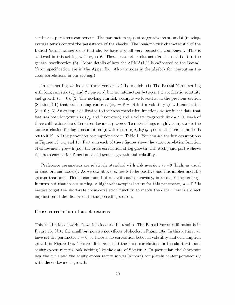
can have a persistent component. The parameters ϕg (autoregressive term) and θ (moving-average term) control the persistence of the shocks. The long-run risk characteristic of theBansal Yaron framework is that shocks have a small very persistent component. This isachieved in this setting with ϕg ≈ θ. These parameters characterize the matrix A in thegeneral specification (6). (More details of how the ARMA(1,1) is calibrated to the Bansal-Yaron specification are in the Appendix. Also includes is the algebra for computing thecross-correlations in our setting.)

In this setting we look at three versions of the model: (1) The Bansal-Yaron settingwith long run risk (ϕg and θ non-zero) but no interaction between the stochastic volatilityand growth (a = 0); (2) The no-long run risk example we looked at in the previous section(Section 4.1) that has no long run risk (ϕg = θ = 0) but a volatility-growth connection(a > 0); (3) An example calibrated to the cross correlation functions we see in the data thatfeatures both long-run risk (ϕg and θ non-zero) and a volatility-growth link a > 0. Each ofthese calibrations is a different endowment process. To make things roughly comparable, theautocorrelation for log consumption growth (corr(log gt, log gt−1)) in all three examples isset to 0.12. All the parameter assumptions are in Table 1. You can see the key assumptionsin Figures 13, 14, and 15. Part a in each of these figures show the auto-correlation functionof endowment growth (i.e., the cross correlation of log growth with itself) and part b showsthe cross-correlation function of endowment growth and volatility.

Preference parameters are relatively standard with risk aversion at −9 (high, as usualin asset pricing models). As we saw above, ρ, needs to be positive and this implies and IESgreater than one. This is common, but not without controversy, in asset pricing settings.It turns out that in our setting, a higher-than-typical value for this parameter, ρ = 0.7 isneeded to get the short-rate cross correlation function to match the data. This is a directimplication of the discussion in the preceding section.

Cross correlation of asset returns

This is all a lot of work. Now, lets look at the results. The Bansal-Yaron calibration is inFigure 13. Note the small but persistence effects of shocks in Figure 13a. In this setting, wehave set the parameter a = 0, so there is no correlation between volatility and consumptiongrowth in Figure 13b. The result here is that the cross correlations in the short rate andequity excess returns look nothing like the data of Section 2. In particular, the short-ratelags the cycle and the equity excess return moves (almost) completely contemporaneouslywith the endowment growth.

20

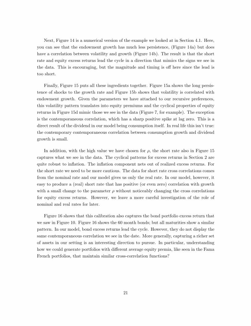
Next, Figure 14 is a numerical version of the example we looked at in Section 4.1. Here,you can see that the endowment growth has much less persistence, (Figure 14a) but doeshave a correlation between volatility and growth (Figure 14b). The result is that the shortrate and equity excess returns lead the cycle in a direction that mimics the signs we see inthe data. This is encouraging, but the magnitude and timing is off here since the lead istoo short.

Finally, Figure 15 puts all these ingredients together. Figure 15a shows the long persis-tence of shocks to the growth rate and Figure 15b shows that volatility is correlated withendowment growth. Given the parameters we have attached to our recursive preferences,this volatility pattern translates into equity premiums and the cyclical properties of equityreturns in Figure 15d mimic those we see in the data (Figure 7, for example). The exceptionis the contemporaneous correlation, which has a sharp positive spike at lag zero. This is adirect result of the dividend in our model being consumption itself. In real life this isn’t true:the contemporary contemporaneous correlation between consumption growth and dividendgrowth is small.

In addition, with the high value we have chosen for ρ, the short rate also in Figure 15captures what we see in the data. The cyclical patterns for excess returns in Section 2 arequite robust to inflation. The inflation component nets out of realized excess returns. Forthe short rate we need to be more cautious. The data for short rate cross correlations comesfrom the nominal rate and our model gives us only the real rate. In our model, however, iteasy to produce a (real) short rate that has positive (or even zero) correlation with growthwith a small change to the parameter ρ without noticeably changing the cross correlationsfor equity excess returns. However, we leave a more careful investigation of the role ofnominal and real rates for later.

Figure 16 shows that this calibration also captures the bond portfolio excess return thatwe saw in Figure 10. Figure 16 shows the 60 month bonds; but all maturities show a similarpattern. In our model, bond excess returns lead the cycle. However, they do not display thesame contemporaneous correlation we see in the date. More generally, capturing a richer setof assets in our setting is an interesting direction to pursue. In particular, understandinghow we could generate portfolios with different average equity premia, like seen in the FamaFrench portfolios, that maintain similar cross-correlation functions?

21

5 Discussion

We have some work to do to nail down the details, but the numerical example shows thatthis kind of mechanism can replicate the shape of cross-correlation functions between excessreturns and economic growth. There remain some open issues. Most of the open issues arefamiliar in asset pricing and unique to our setting.

Risk and risk aversion. We’ve mimicked the cyclical behavior of excess returns in a modelin which expected excess returns stem from variations in risk with constant risk aversion.We could have addressed the same issue by allowing risk aversion to vary across states,as it does in Campbell and Cochrane (1999) and Routledge and Zin (2010), or by lettingthe price of risk vary with the distribution of wealth across individuals, as in Lustig andVan Nieuwerburgh (2005) or Guvenen (2009). We have no particular reason to prefer ourapproach to these alternatives. Our point is simply that the data implies cyclical variationin excess returns. Exactly how different source of cyclical variation, beyond stochasticvolatility, can be correlated with growth might be interesting to consider.

A related issue is the magnitude of risk aversion used in our example. A common argu-ment against risk aversion parameters this large is that when we extrapolate them to largerisks (aggregate risks are small), the extent of risk aversion seems unreasonable. Extrapola-tion of this sort depends a lot on the form of risk preference, including the power form usedhere and expected utility in general. A natural resolution is a form of risk preference thatexhibits different aversion to small and large risks. One such is disappointment aversion.Campanale, Castro, and Clementi (2006) show that the first-order risk aversion exhibitedby such preferences exhibits substantial aversion to the small risks we see in the aggregateyet has modest aversion to the large risks faced by individuals. We could model that ex-plicitly in this case, but at some cost of computational complexity. It’s simpler to think ofour risk preferences as a local approximation for the small risks present in this model.

An alternative is to interpret the risk aversion parameter as aversion to uncertaintyabout the model’s structure. Barillas, Hansen, and Sargent (2008) show that a modestamount of uncertainty about the model’s structure (the stochastic process for consumption,for example) can look like extreme risk aversion.

Consumption and returns. Empirical work by Canzoneri, Dumby, and Diba (2007) andParker and Julliard (2005) shows that the contemporaneous correlation between returns andconsumption growth is small, but increases as we expand the time interval. The evidenceis Sections 2 is similar: since the correlation is larger with a lag of several months, it’s not

22

hard to imagine that the correlation will increase with the time interval. Our theoreticalmodel suggestions an explanation: that the pricing kernel contains an additional factor thatis correlated with consumption growth only with a lag.

Alvarez-Jermann bound. Our example has a relatively small bound. Is there enough vari-ability in the pricing kernel with our parameter values?

Endogenous consumption. In a more complete model, variation in the conditional varianceof (say) productivity shocks will generate an endogenous response from consumption. Naik(1993) and Primiceri, Schaumburg, Tambalotti (2006) are examples. It remains to be seenwhether this produces the interaction we have specified for volatility and consumptiongrowth. Some details on how the lead-lag relationship might work in a production settingwith recursive preferences is in Backus, Routledge, and Zin (2007).

Cross-section of returns. We’ve looked at the possibility that aggregate volatility mightaccount for the cyclical behavior of excess returns. Koijen, Lustig, and Van Nieuwerburgh(2008) use a similar approach to account for the cross section of asset returns.

.

Solution method. There is a growing literature on perturbation methods, in which uncer-tainty doesn’t appear until the second-order approximation. Collard and Juillard (2001) isan elegant example, and Van Binsbergen, Fernandez-Villaverde, Koijen, and Rubio-Ramirez(2008) show how such methods can be extended to models with recursive preferences. Ourapproach differs in two respects: recursive preferences lead to more complex equilibriumconditions, and we use methods similar to those in finance in which variances appear evenwith first-order (linear) approximations. This isn’t a substitute for high-order approxi-mations, but it allows us to generate reasonably accurate solutions without giving up theconvenience of linearity.

6 Conclusions

In short: The returns data suggest that excess returns lead the business cycle by 6-9 months.We replicate this feature in an exchange economy that has a few key features: Recursive pref-erences; an endowment process that has predictable variation in both consumption growthand its conditional variance; and where predictability in consumption growth depends onpast volatility. All of these features are necessary to account for the cyclical behavior of theexcess returns, and in particular, the equity premium.

23

A Data sources

[Later.]

B Theoretical results

The Kreps-Porteus pricing kernel

The pricing kernel in a representative agent model is the marginal rate of substitutionbetween (say) consumption at date t [ct] and consumption in state s at t+1 [ct+1(s)]. Here’show that works with recursive preferences. With this notation, the certainty equivalent (3)might be expressed less compactly as

µt(Ut+1) =

[∑s

π(s)Ut+1(s)α]1/α

,

where π(s) is the conditional probability of state s and Ut+1(s) is continuation utility. Somederivatives of (2) and (3):

∂Ut/∂ct = U1−ρt (1− β)cρ−1

t

∂Ut/∂µt(Ut+1) = U1−ρt βµt(Ut+1)ρ−1

∂µt(Ut+1)/∂Ut+1(s) = µt(Ut+1)1−απ(s)Ut+1(s)α−1.

The marginal rate of substitution between consumption at date t and consumption in states at t+ 1 is

∂Ut/∂ct+1(s)∂Ut/∂ct

=[∂Ut/∂µt(Ut+1)][∂µt(Ut+1)/∂Ut+1(s)][∂Ut+1(s)/∂ct+1(s)]

∂Ut/∂ct

= π(s) β(ct+1(s)ct

)ρ−1 ( Ut+1(s)µt(Ut+1)

)α−ρ.

The pricing kernel (5) is the same with the probability π(s) left out and the state leftimplicit.

Equity prices and returns

We define equity at t as a claim to consumption from t + 1 on. The return is the ratio ofits value at t + 1, measured in units of t + 1 consumption, to the value at t, measured inunits of t consumption. The value at t+ 1 is Ut+1 expressed in ct+1 units:

Ut+1/ (∂Ut+1/∂ct+1) = Ut+1/[(1− β)U1−ρ

t+1 cρ−1t+1

]= (1− β)−1uρt+1ct+1.

24

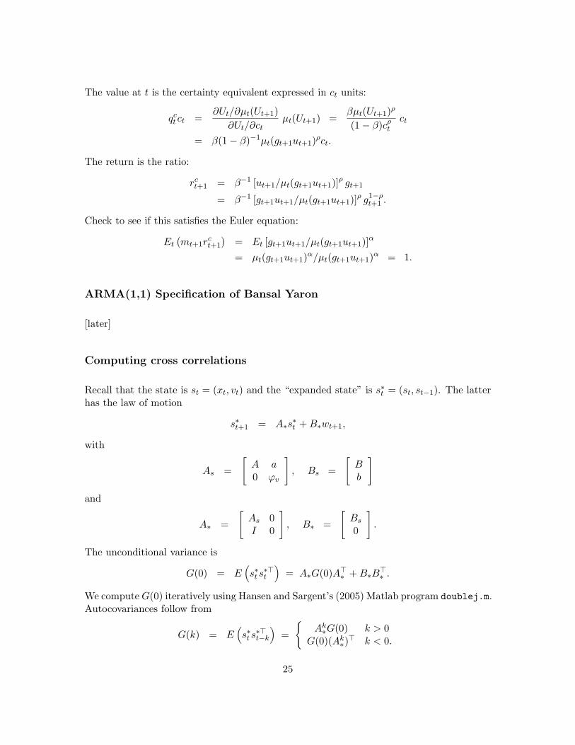
The value at t is the certainty equivalent expressed in ct units:

qct ct =∂Ut/∂µt(Ut+1)

∂Ut/∂ctµt(Ut+1) =

βµt(Ut+1)ρ

(1− β)cρtct

= β(1− β)−1µt(gt+1ut+1)ρct.

The return is the ratio:

rct+1 = β−1 [ut+1/µt(gt+1ut+1)]ρ gt+1

= β−1 [gt+1ut+1/µt(gt+1ut+1)]ρ g1−ρt+1 .

Check to see if this satisfies the Euler equation:

Et(mt+1r

ct+1

)= Et [gt+1ut+1/µt(gt+1ut+1)]α

= µt(gt+1ut+1)α/µt(gt+1ut+1)α = 1.

ARMA(1,1) Specification of Bansal Yaron

[later]

Computing cross correlations

Recall that the state is st = (xt, vt) and the “expanded state” is s∗t = (st, st−1). The latterhas the law of motion

s∗t+1 = A∗s∗t +B∗wt+1,

with

As =

[A a0 ϕv

], Bs =

[Bb

]

and

A∗ =

[As 0I 0

], B∗ =

[Bs0

].

The unconditional variance is

G(0) = E(s∗t s∗>t

)= A∗G(0)A>∗ +B∗B

>∗ .

We computeG(0) iteratively using Hansen and Sargent’s (2005) Matlab program doublej.m.Autocovariances follow from

G(k) = E(s∗t s∗>t−k

)=

{Ak∗G(0) k > 0

G(0)(Ak∗)> k < 0.

25

Since G(−k) = G(k)>, positive k is sufficient.

Returns and excess returns are linear functions of the expanded state: rt = Hs∗t say fora vector of returns and excess returns. Autocovariances are

E(rtr>t−k

)= hG(k)h>.

Cross-covariances are off-diagonal elements and cross-correlations are scaled by standarddeviations.

26

References

Alvarez, Fernando, and Urban Jermann, 2005, “Using asset prices to measure the persistenceof the marginal utility of wealth,” Econometrica 73, 1977-2016.

Ang, Andrew, Monika Piazzesi, and Min Wei, 2006, “What does the yield curve tell usabout GDP growth?” Journal of Econometrics 131, 359-403.

Atkeson, Andrew, and Patrick Kehoe, 2008, “On the need for a new approach to analyzingmonetary policy,” NBER Macroeconomics Annual , forthcoming.

Backus, David K., Bryan R. Routledge, and Stanley E. Zin, 2007, “Asset prices in businesscycle analysis,” manuscript, November.

Bansal, Ravi, and Amir Yaron, 2004, “Risks for the long run: A potential resolution ofasset pricing puzzles,” Journal of Finance 59, 1481-1509.

Barillas, Francisco, Lars Peter Hansen, and Thomas J. Sargent, 2008, “Doubts or variabil-ity,” manuscript, July.

Campanale, Claudio, Rui Castro, and Gian Luca Clementi, 2006, “Asset pricing in a gen-eral equilibrium production economy with Chew-Dekel risk preferences,” manuscript,December.

Campbell, John Y., and John H. Cochrane, 1999, “By force of habit: a consumption-basedexplanation of aggregate stock market behavior,” Journal of Political Economy 107,205-251.

Canzoneri, Matthew B., Robert E. Cumby, and Behzad T. Diba, 2007, “Euler equationsand money market interest rates: a challenge for monetary policy models,” Journalof Monetary Economics 54, 1863-1881.

Casassus, Jaime, Peng Liu and Ke Tang, 2010, Long-term economic relationships and cor-relation structure in commodity markets, Pontificia Universidad Catolica de ChileWorking Paper, February, 2010.

Constantinides, George M. and Anisha Ghosh, 2010, “The Predictability of Returns withRegime Shifts in Consumption and Dividend Growth,” Carnegie Mellon WorkingPaper, January, 2010

Collard, Fabrice, and Michel Juillard, 2001, “Accuracy of stochastic perturbation methods:the case of asset pricing models,” Journal of Economic Dynamics and Control 25,979-999.

Epstein, Larry G., and Stanley E. Zin, 1989, “Substitution, risk aversion, and the temporalbehavior of consumption and asset returns: a theoretical framework,” Econometrica57, 937-969.

Estrella, Arturo, and Gikas A. Hardouvelis, 1991, “The term structure as a predictor of realeconomic activity,” Journal of Finance 46, 555-576.

Fama, Eugene F., and Kenneth R. French, 1989, “Business conditions and expected returnson stocks and bonds,” Journal of Monetary Economics 25, 23-49.

Fama, Eugene F., and Kenneth R. French, 1992, “The cross-section of expected stock

27

returns,” Journal of Finance 47, 427-467.Gallmeyer, Michael F., Burton Hollifield, and Stanley E. Zin, 2005, “Taylor rules, McCallum

rules and the term structure of interest rates,” Journal of Monetary Economics 52,921-950.

Guvenen, Fatih 2009, A Parsimonious Macroeconomic Model for Asset Pricing* Economet-rica, November 2009, Vol. 77, No 6, pp. 1711-1750.

Hansen, Lars Peter, John C. Heaton, and Nan Li, 2008, “Consumption strikes back? Mea-suring long-run risk,” Journal of Political Economy 116, 260-302.

Hansen, Lars Peter, and Thomas J. Sargent, 2005, Recursive Models of Dynamic LinearEconomies, manuscript, September.

Parker, Jonathan A., and Christian Julliard, 2005, “Consumption risk and the cross sectionof expected returns,” Journal of Political Economy 113, 185-222.

Kandel, Shmuel, Robert F. Stambaugh, 1990, “Expectations and volatility of consumptionand asset returns,” Review of Financial Studies 3, 207-32.

King, Robert G., and Mark W. Watson, 1996, “Money, prices, interest rates and the businesscycle,” Review of Economics and Statistics 78, 35-53.

Koijen, Ralph, Hanno Lustig, and Stijn Van Nieuwerburgh, 2008, “The bond risk premiumand the cross-section of expected stock returns,” manuscript.

Kreps, David M., and Evan L. Porteus, 1978, “Temporal resolution of uncertainty anddynamic choice theory,” Econometrica 46, 185-200.

Lustig, Hanno, and Stijn Van Nieuwerburgh, 2005, “Housing collateral, consumption insur-ance and risk premia: an empirical perspective,” Journal of Finance 60, 1167-1219.

Mueller, Philippe, 2008, “Credit spreads and real activity,” manuscript, London School ofEconomics, January.

Naik, Vasanttilak, 1994, “Asset prices in time-varying production economies with time-varying risk,” Review of Financial Studies 7, 781-801.

Primiceri, Giorgio E., Ernst Schaumburg, and Andrea Tambalotti, 2006, “Intertemporaldisturbances,” NBER Working Paper 12243, May.

Routledge, Bryan R., and Stanley E. Zin, 2010, “Generalized disappointment aversion andasset prices,” Journal of Finance , Volume 65, 4

Rouwenhorst, K. Geert, 1995, “Asset pricing implications of equilibrium business cyclemodels,” in T.F. Cooley, editor, Frontiers of Business Cycle Research, Princeton,NJ: Princeton University Press.

Sargent, Thomas J., and Christopher A. Sims, 1977, “Business cycle modeling withoutpretending to have too much a priori economic theory,” in C. Sims et al., eds.,New Methods in Business Cycle Research, Minneapolis: Federal Reserve Bank ofMinneapolis.

Stock, James H., and Mark W. Watson, 1989, “New indexes of coincident and leadingeconomic indicators,” in NBER Macroeconomics Annual , O.J. Blanchard and S.Fischer, eds., 352-394.

28

Stock, James H., and Mark W. Watson, 2003, “Forecasting output and inflation: the roleof asset prices,” Journal of Economic Literature 41, 788-829.

Stock, James H., and Mark W. Watson, 2005, “Implications of dynamic factor models forVAR analysis,” NBER Working Paper No. 11467, June.

van Binsbergen, Jules, Jesus Fernandez-Villaverde, Ralph Koijen, and Juan Rubio-Ramirez,2008, “Likelihood estimation of DSGE models with Epstein-Zin preferences,” manuscript,March.

Weil, Philippe, 1989, “The equity premium puzzle and the risk-free rate puzzle,” Journalof Monetary Economics 24, 401-421.

29

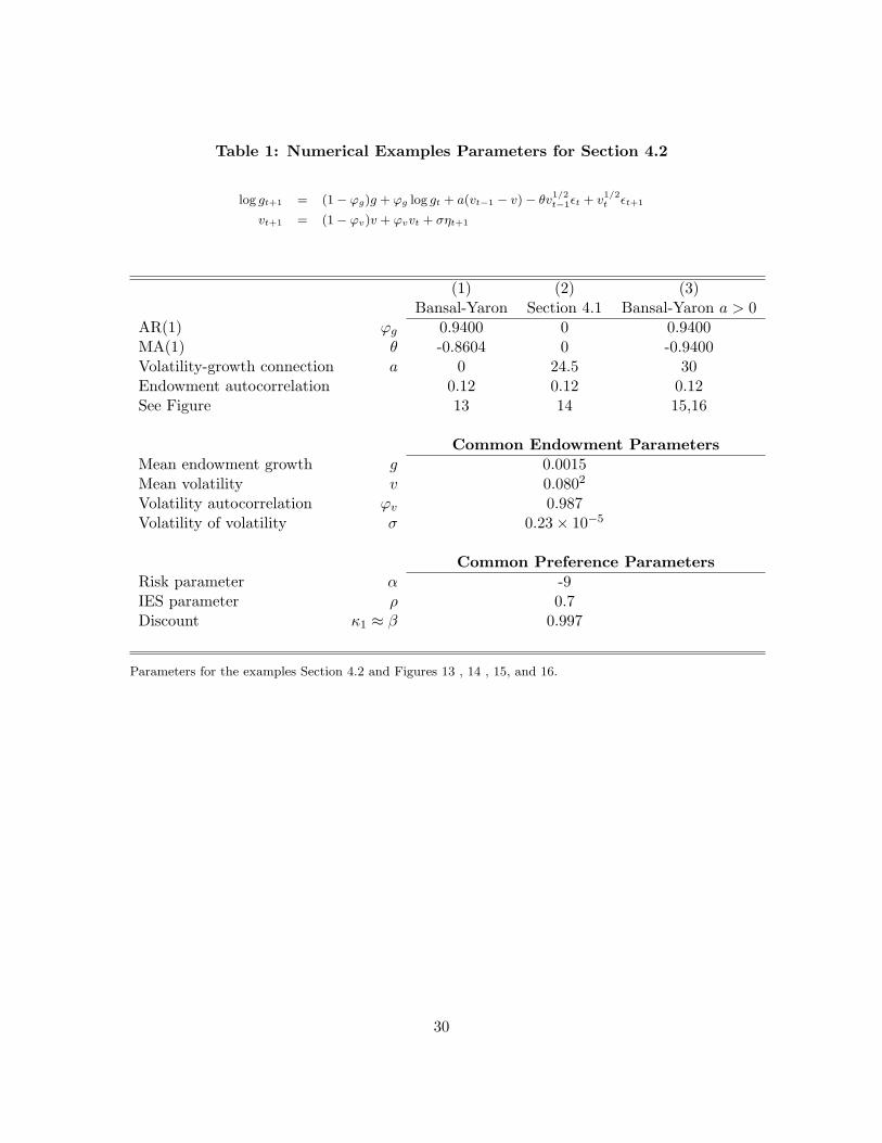
Table 1: Numerical Examples Parameters for Section 4.2

log gt+1 = (1− ϕg)g + ϕg log gt + a(vt−1 − v)− θv1/2t−1εt + v

1/2t εt+1

vt+1 = (1− ϕv)v + ϕvvt + σηt+1

(1) (2) (3)Bansal-Yaron Section 4.1 Bansal-Yaron a > 0

AR(1) ϕg 0.9400 0 0.9400MA(1) θ -0.8604 0 -0.9400Volatility-growth connection a 0 24.5 30Endowment autocorrelation 0.12 0.12 0.12See Figure 13 14 15,16

Common Endowment ParametersMean endowment growth g 0.0015Mean volatility v 0.0802

Volatility autocorrelation ϕv 0.987Volatility of volatility σ 0.23× 10−5

Common Preference ParametersRisk parameter α -9IES parameter ρ 0.7Discount κ1 ≈ β 0.997

Parameters for the examples Section 4.2 and Figures 13 , 14 , 15, and 16.

30

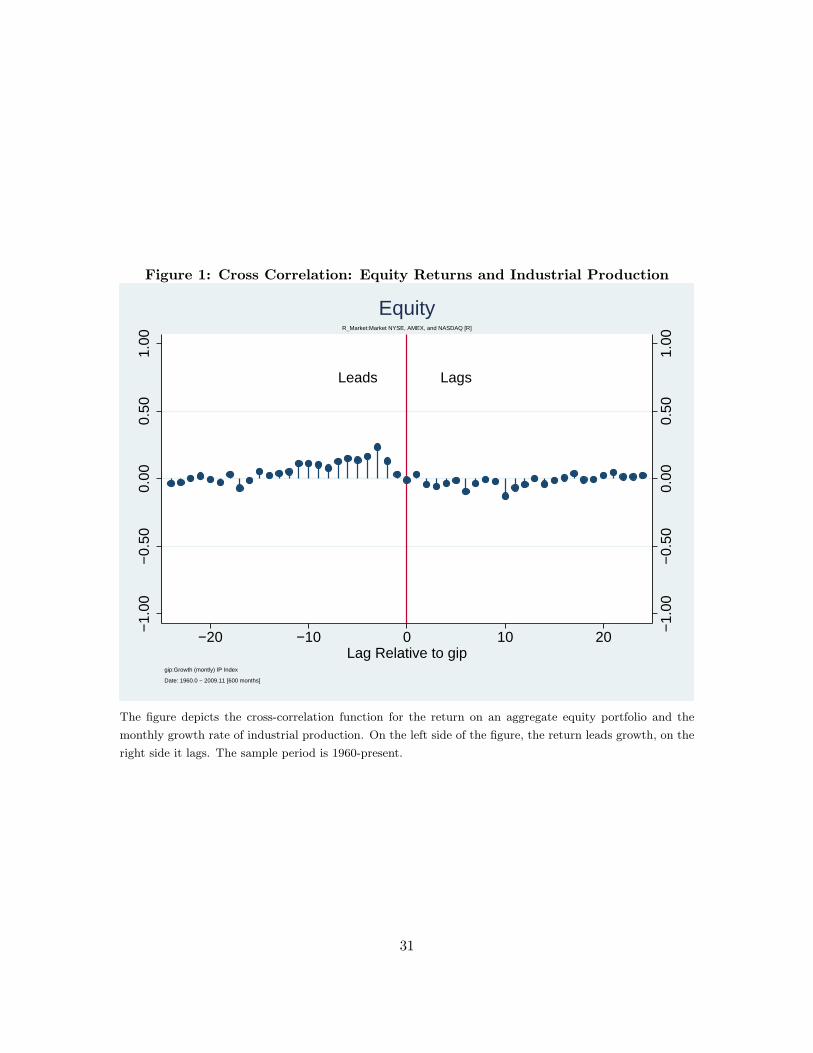
Figure 1: Cross Correlation: Equity Returns and Industrial Production

Leads Lags

−1.

00−

0.50

0.00

0.50

1.00

−1.

00−

0.50

0.00

0.50

1.00

−20 −10 0 10 20Lag Relative to gip

gip:Growth (montly) IP Index

Date: 1960.0 − 2009.11 [600 months]

R_Market:Market NYSE, AMEX, and NASDAQ [R]

Equity

The figure depicts the cross-correlation function for the return on an aggregate equity portfolio and the

monthly growth rate of industrial production. On the left side of the figure, the return leads growth, on the

right side it lags. The sample period is 1960-present.

31

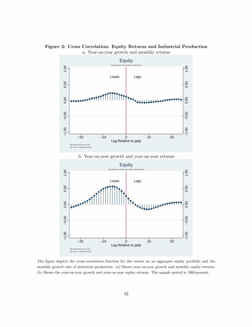
Figure 2: Cross Correlation: Equity Returns and Industrial Productiona. Year-on-year growth and monthly returns

Leads Lags

−1.

00−

0.50

0.00

0.50

1.00

−1.

00−

0.50

0.00

0.50

1.00

−20 −10 0 10 20Lag Relative to gaip

gaip:Growth (annual yoy) IP Index

Date: 1960.0 − 2009.6 [595 months]


Equity

b. Year-on-year growth and year-on-year returns

Leads Lags

−1.

00−

0.50

0.00

0.50

1.00

−1.

00−

0.50

0.00

0.50

1.00



Date: 1960.0 − 2009.5 [594 months]

ga_R_Market:yoy er Market NYSE, AMEX, and NASDAQ [R]

Equity


monthly growth rate of industrial production. (a) Shows year-on-year growth and monthly equity returns.

(b) Shows the year-on-year growth and year-on-year equity returns. The sample period is 1960-present.

32

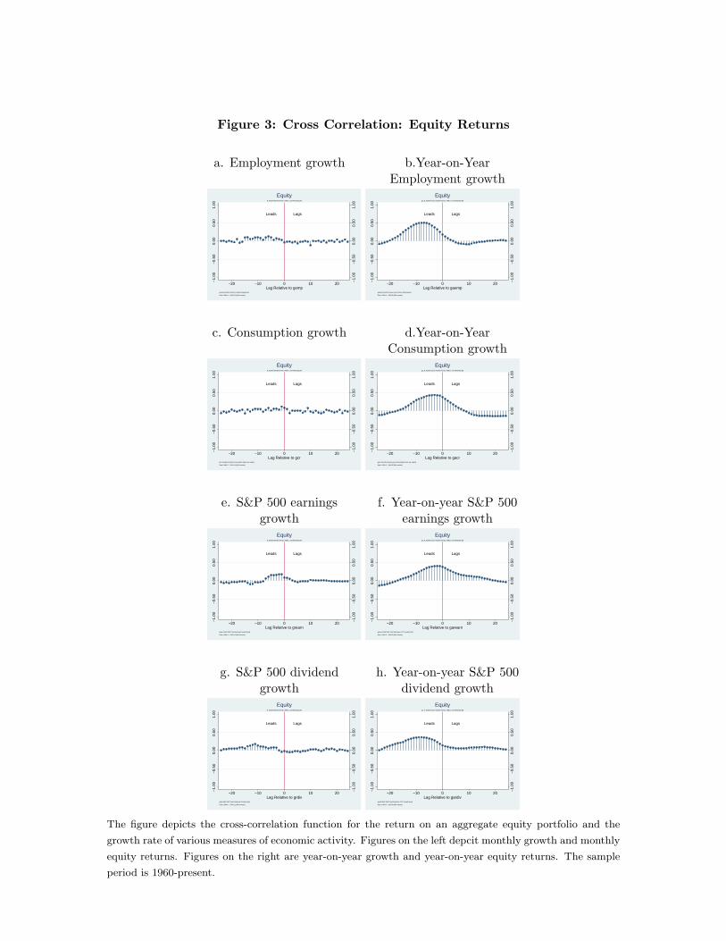
Figure 3: Cross Correlation: Equity Returns

a. Employment growth b.Year-on-YearEmployment growth

Leads Lags

−1.

00−

0.50

0.00

0.50

1.00

−1.

00−

0.50

0.00

0.50

1.00

−20 −10 0 10 20Lag Relative to gemp

gemp:Growth (montly) Civilian Employment

Date: 1960.0 − 2009.11 [600 months]


Equity

Leads Lags

−1.

00−

0.50

0.00

0.50

1.00

−1.

00−

0.50

0.00

0.50

1.00

−20 −10 0 10 20Lag Relative to gaemp

gaemp:Growth (annual yoy) Civilian Employment

Date: 1960.0 − 2009.5 [594 months]


Equity

c. Consumption growth d.Year-on-YearConsumption growth

Leads Lags

−1.

00−

0.50

0.00

0.50

1.00

−1.

00−

0.50

0.00

0.50

1.00

−20 −10 0 10 20Lag Relative to gcr

gcr:Growth (montly) Consumption [real; per capita]

Date: 1960.0 − 2009.11 [600 months]


Equity

Leads Lags

−1.

00−

0.50

0.00

0.50

1.00

−1.

00−

0.50

0.00

0.50

1.00

−20 −10 0 10 20Lag Relative to gacr

gacr:Growth (annual yoy) Consumption [real; per capita]

Date: 1960.0 − 2009.5 [594 months]


Equity

e. S&P 500 earningsgrowth

f. Year-on-year S&P 500earnings growth

Leads Lags

−1.

00−

0.50

0.00

0.50

1.00

−1.

00−

0.50

0.00

0.50

1.00

−20 −10 0 10 20Lag Relative to grearn

grearn:S&P 500 Total Earnings Growth [real]

Date: 1960.0 − 2009.11 [600 months]


Equity

Leads Lags

−1.

00−

0.50

0.00

0.50

1.00

−1.

00−

0.50

0.00

0.50

1.00

−20 −10 0 10 20Lag Relative to garearn

garearn:S&P 500 Total Earnings YOY Growth [real]

Date: 1960.0 − 2009.5 [594 months]


Equity

g. S&P 500 dividendgrowth

h. Year-on-year S&P 500dividend growth

Leads Lags

−1.

00−

0.50

0.00

0.50

1.00

−1.

00−

0.50

0.00

0.50

1.00

−20 −10 0 10 20Lag Relative to grdiv

grdiv:S&P 500 Total Dividends Growth [real]

Date: 1960.0 − 2009.11 [600 months]


Equity

Leads Lags

−1.

00−

0.50

0.00

0.50

1.00

−1.

00−

0.50

0.00

0.50

1.00

−20 −10 0 10 20Lag Relative to gardiv

gardiv:S&P 500 Total Dividends YOY Growth [real]

Date: 1960.0 − 2009.5 [594 months]


Equity


growth rate of various measures of economic activity. Figures on the left depcit monthly growth and monthly

equity returns. Figures on the right are year-on-year growth and year-on-year equity returns. The sample

period is 1960-present.

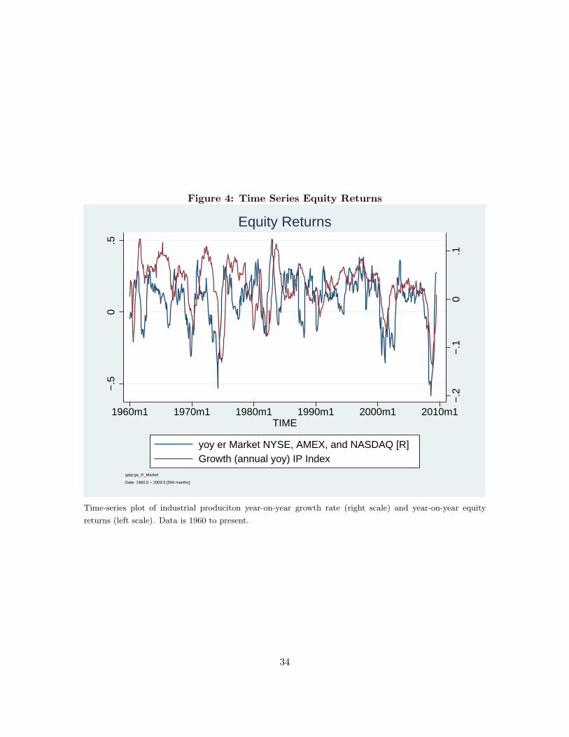
Figure 4: Time Series Equity Returns

−.2

−.1

0.1

−.5

0.5

1960m1 1970m1 1980m1 1990m1 2000m1 2010m1TIME

yoy er Market NYSE, AMEX, and NASDAQ [R]Growth (annual yoy) IP Index

gaip:ga_R_Market

Date: 1960.0 − 2009.5 [594 months]

Equity Returns

Time-series plot of industrial produciton year-on-year growth rate (right scale) and year-on-year equity

returns (left scale). Data is 1960 to present.

34

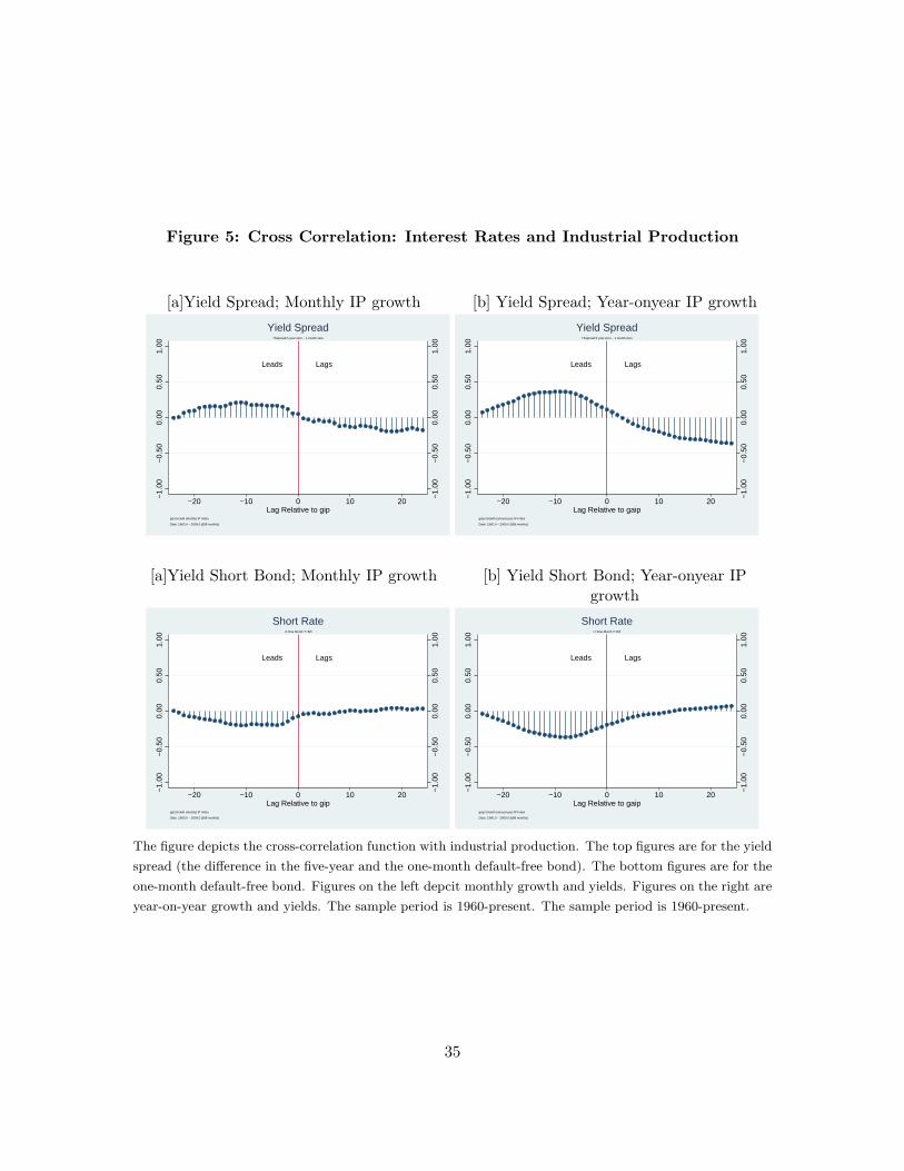
Figure 5: Cross Correlation: Interest Rates and Industrial Production

[a]Yield Spread; Monthly IP growth [b] Yield Spread; Year-onyear IP growth

Leads Lags

−1.

00−

0.50

0.00

0.50

1.00

−1.

00−

0.50

0.00

0.50

1.00



Date: 1960.0 − 2009.0 [588 months]

TSspread:5 year zero − 1 month zero

Yield Spread

Leads Lags

−1.

00−

0.50

0.00

0.50

1.00

−1.

00−

0.50

0.00

0.50

1.00



Date: 1960.0 − 2009.0 [588 months]

TSspread:5 year zero − 1 month zero

Yield Spread

[a]Yield Short Bond; Monthly IP growth [b] Yield Short Bond; Year-onyear IPgrowth

Leads Lags

−1.

00−

0.50

0.00

0.50

1.00

−1.

00−

0.50

0.00

0.50

1.00



Date: 1960.0 − 2009.0 [588 months]

r1:One Month T−Bill

Short Rate

Leads Lags

−1.

00−

0.50

0.00

0.50

1.00

−1.

00−

0.50

0.00

0.50

1.00



Date: 1960.0 − 2009.0 [588 months]

r1:One Month T−Bill

Short Rate

The figure depicts the cross-correlation function with industrial production. The top figures are for the yield

spread (the difference in the five-year and the one-month default-free bond). The bottom figures are for the

one-month default-free bond. Figures on the left depcit monthly growth and yields. Figures on the right are

year-on-year growth and yields. The sample period is 1960-present. The sample period is 1960-present.

35

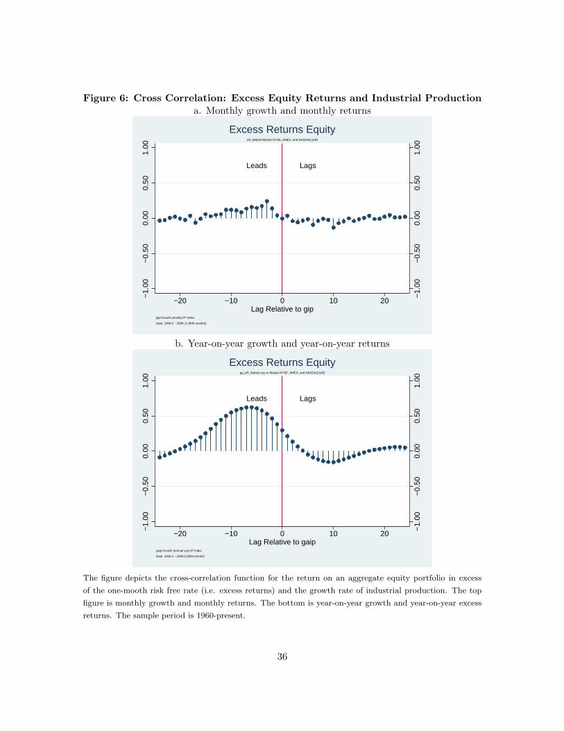
Figure 6: Cross Correlation: Excess Equity Returns and Industrial Productiona. Monthly growth and monthly returns

Leads Lags

−1.

00−

0.50

0.00

0.50

1.00

−1.

00−

0.50

0.00

0.50

1.00



Date: 1960.0 − 2009.11 [600 months]

eR_Market:Market NYSE, AMEX, and NASDAQ [eR]

Excess Returns Equity

b. Year-on-year growth and year-on-year returns

Leads Lags

−1.

00−

0.50

0.00

0.50

1.00

−1.

00−

0.50

0.00

0.50

1.00



Date: 1960.0 − 2009.5 [594 months]

ga_eR_Market:yoy er Market NYSE, AMEX, and NASDAQ [eR]

Excess Returns Equity

The figure depicts the cross-correlation function for the return on an aggregate equity portfolio in excess

of the one-mooth risk free rate (i.e. excess returns) and the growth rate of industrial production. The top

figure is monthly growth and monthly returns. The bottom is year-on-year growth and year-on-year excess

returns. The sample period is 1960-present.

36

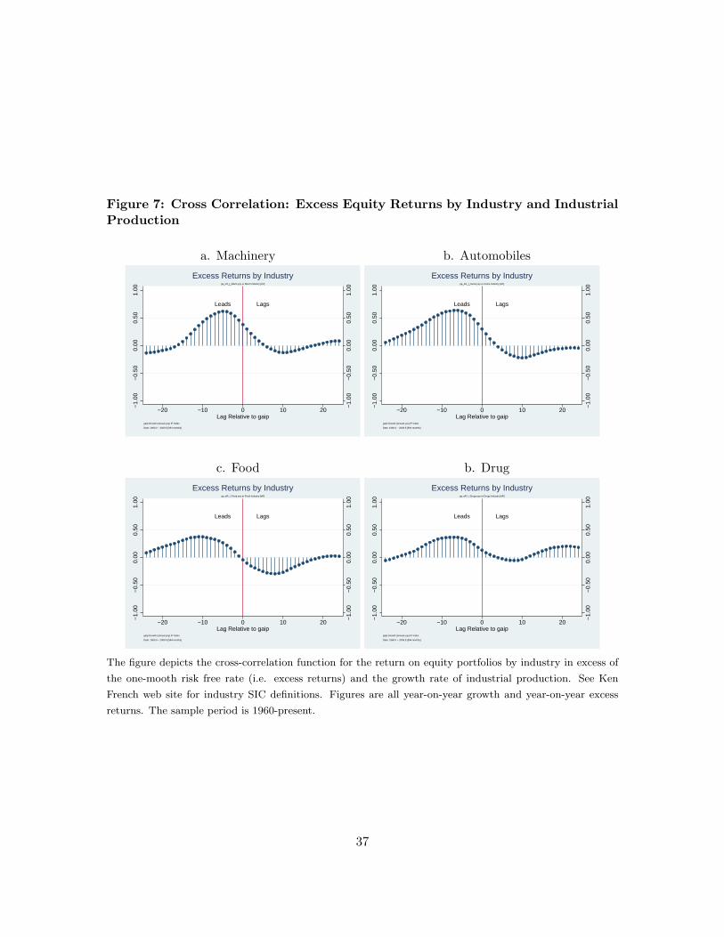
Figure 7: Cross Correlation: Excess Equity Returns by Industry and IndustrialProduction

a. Machinery b. Automobiles

Leads Lags

−1.

00−

0.50

0.00

0.50

1.00

−1.

00−

0.50

0.00

0.50

1.00



Date: 1960.0 − 2009.5 [594 months]

ga_eR_I_Mach:yoy er Mach Industry [eR]

Excess Returns by Industry

Leads Lags

−1.

00−

0.50

0.00

0.50

1.00

−1.

00−

0.50

0.00

0.50

1.00



Date: 1960.0 − 2009.5 [594 months]

ga_eR_I_Autos:yoy er Autos Industry [eR]


c. Food b. Drug

Leads Lags

−1.

00−

0.50

0.00

0.50

1.00

−1.

00−

0.50

0.00

0.50

1.00



Date: 1960.0 − 2009.5 [594 months]

ga_eR_I_Food:yoy er Food Industry [eR]


Leads Lags

−1.

00−

0.50

0.00

0.50

1.00

−1.

00−

0.50

0.00

0.50

1.00



Date: 1960.0 − 2009.5 [594 months]

ga_eR_I_Drugs:yoy er Drugs Industry [eR]


The figure depicts the cross-correlation function for the return on equity portfolios by industry in excess of

the one-mooth risk free rate (i.e. excess returns) and the growth rate of industrial production. See Ken

French web site for industry SIC definitions. Figures are all year-on-year growth and year-on-year excess

returns. The sample period is 1960-present.

37

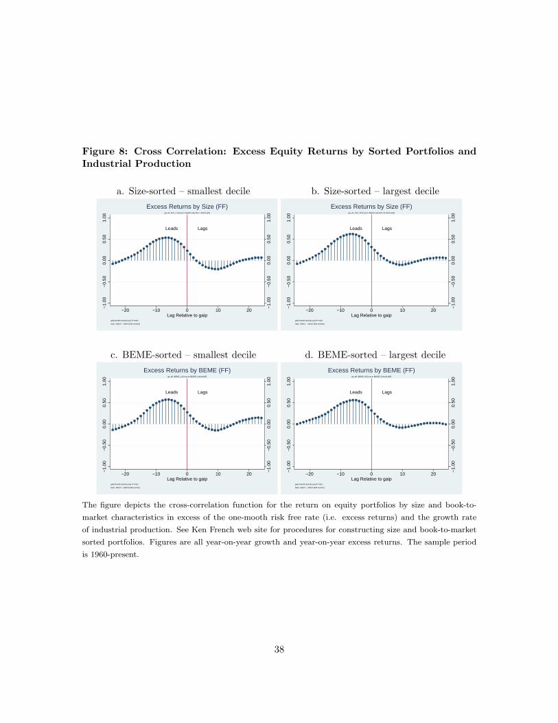
Figure 8: Cross Correlation: Excess Equity Returns by Sorted Portfolios andIndustrial Production

a. Size-sorted – smallest decile b. Size-sorted – largest decile

Leads Lags

−1.

00−

0.50

0.00

0.50

1.00

−1.

00−

0.50

0.00

0.50

1.00



Date: 1960.0 − 2009.5 [594 months]

ga_eR_Size_Lo10:yoy er Market Cap Size 1 Decile [eR]

Excess Returns by Size (FF)

Leads Lags

−1.

00−

0.50

0.00

0.50

1.00

−1.

00−

0.50

0.00

0.50

1.00



Date: 1960.0 − 2009.5 [594 months]

ga_eR_Size_Hi10:yoy er Market Cap Size 10 Decile [eR]

Excess Returns by Size (FF)

c. BEME-sorted – smallest decile d. BEME-sorted – largest decile

Leads Lags

−1.

00−

0.50

0.00

0.50

1.00

−1.

00−

0.50

0.00

0.50

1.00



Date: 1960.0 − 2009.5 [594 months]

ga_eR_BEME_Lo10:yoy er BE/ME 1 decile [eR]

Excess Returns by BEME (FF)

Leads Lags

−1.

00−

0.50

0.00

0.50

1.00

−1.

00−

0.50

0.00

0.50

1.00



Date: 1960.0 − 2009.5 [594 months]

ga_eR_BEME_Hi10:yoy er BE/ME 10 decile [eR]

Excess Returns by BEME (FF)

The figure depicts the cross-correlation function for the return on equity portfolios by size and book-to-

market characteristics in excess of the one-mooth risk free rate (i.e. excess returns) and the growth rate

of industrial production. See Ken French web site for procedures for constructing size and book-to-market

sorted portfolios. Figures are all year-on-year growth and year-on-year excess returns. The sample period

is 1960-present.

38

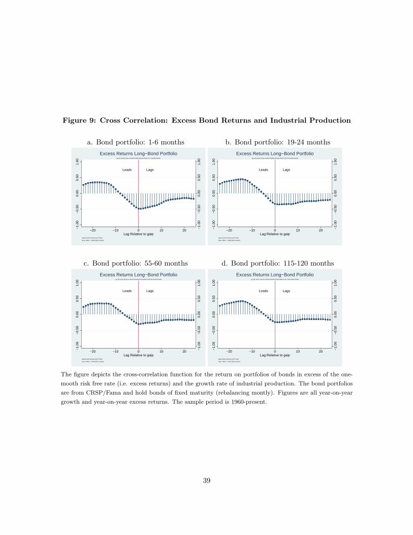
Figure 9: Cross Correlation: Excess Bond Returns and Industrial Production

a. Bond portfolio: 1-6 months b. Bond portfolio: 19-24 months

Leads Lags

−1.

00−

0.50

0.00

0.50

1.00

−1.

00−

0.50

0.00

0.50

1.00



Date: 1960.0 − 2008.5 [582 months]

ga_eR_bond_6:yoy er Bond Portfolio Excess Return (1−6 months bonds)

Excess Returns Long−Bond Portfolio

Leads Lags

−1.

00−

0.50

0.00

0.50

1.00

−1.

00−

0.50

0.00

0.50

1.00



Date: 1960.0 − 2008.5 [576 months]



c. Bond portfolio: 55-60 months d. Bond portfolio: 115-120 months

Leads Lags

−1.

00−

0.50

0.00

0.50

1.00

−1.

00−

0.50

0.00

0.50

1.00



Date: 1960.0 − 2008.5 [557 months]



Leads Lags

−1.

00−

0.50

0.00

0.50

1.00

−1.

00−

0.50

0.00

0.50

1.00



Date: 1960.0 − 2008.5 [582 months]



The figure depicts the cross-correlation function for the return on portfolios of bonds in excess of the one-

mooth risk free rate (i.e. excess returns) and the growth rate of industrial production. The bond portfolios

are from CRSP/Fama and hold bonds of fixed maturity (rebalancing montly). Figures are all year-on-year

growth and year-on-year excess returns. The sample period is 1960-present.

39

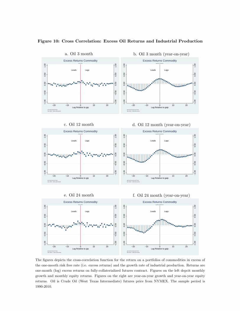
Figure 10: Cross Correlation: Excess Oil Returns and Industrial Production

a. Oil 3 month b. Oil 3 month (year-on-year)

Leads Lags

−1.

00−

0.50

0.00

0.50

1.00

−1.

00−

0.50

0.00

0.50

1.00



Date: 1990.0 − 2009.11 [239 months]

eR_F_CL3:

Excess Returns Commodity

Leads Lags

−1.

00−

0.50

0.00

0.50

1.00

−1.

00−

0.50

0.00

0.50

1.00



Date: 1990.6 − 2009.5 [226 months]

ga_eR_F_CL3:yoy er


c. Oil 12 month d. Oil 12 month (year-on-year)

Leads Lags

−1.

00−

0.50

0.00

0.50

1.00

−1.

00−

0.50

0.00

0.50

1.00



Date: 1990.0 − 2009.11 [236 months]

eR_F_CL12:


Leads Lags

−1.

00−

0.50

0.00

0.50

1.00

−1.

00−

0.50

0.00

0.50

1.00



Date: 1990.6 − 2009.5 [221 months]

ga_eR_F_CL12:yoy er


e. Oil 24 month f. Oil 24 month (year-on-year)

Leads Lags

−1.

00−

0.50

0.00

0.50

1.00

−1.

00−

0.50

0.00

0.50

1.00



Date: 1990.11 − 2009.11 [202 months]

eR_F_CL24:


Leads Lags

−1.

00−

0.50

0.00

0.50

1.00

−1.

00−

0.50

0.00

0.50

1.00



Date: 1991.5 − 2009.5 [178 months]

ga_eR_F_CL24:yoy er


The figures depicts the cross-correlation function for the return on a portfolios of commodities in excess of

the one-mooth risk free rate (i.e. excess returns) and the growth rate of industrial production. Returns are

one-month (log) excess returns on fully-collaterialized futures contract. Figures on the left depcit monthly

growth and monthly equity returns. Figures on the right are year-on-year growth and year-on-year equity

returns. Oil is Crude Oil (West Texas Intermediate) futures price from NYMEX. The sample period is

1990-2010.

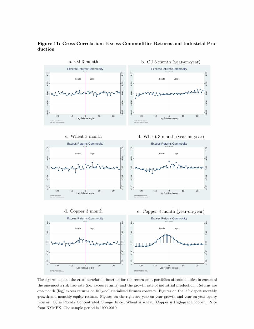
Figure 11: Cross Correlation: Excess Commodities Returns and Industrial Pro-duction

a. OJ 3 month b. OJ 3 month (year-on-year)

Leads Lags

−1.

00−

0.50

0.00

0.50

1.00

−1.

00−

0.50

0.00

0.50

1.00



Date: 1990.0 − 2009.11 [140 months]

eR_F_OJ3:


Leads Lags

−1.

00−

0.50

0.00

0.50

1.00

−1.

00−

0.50

0.00

0.50

1.00



Date: 1990.6 − 2009.3 [124 months]

ga_eR_F_OJ3:yoy er


c. Wheat 3 month d. Wheat 3 month (year-on-year)

Leads Lags

−1.

00−

0.50

0.00

0.50

1.00

−1.

00−

0.50

0.00

0.50

1.00



Date: 1990.0 − 2009.11 [118 months]

eR_F_W3:


Leads Lags

−1.

00−

0.50

0.00

0.50

1.00

−1.

00−

0.50

0.00

0.50

1.00



Date: 1990.6 − 2009.2 [102 months]

ga_eR_F_W3:yoy er


d. Copper 3 month e. Copper 3 month (year-on-year)

Leads Lags

−1.

00−

0.50

0.00

0.50

1.00

−1.

00−

0.50

0.00

0.50

1.00



Date: 1990.0 − 2009.11 [239 months]

eR_F_HG3:


Leads Lags

−1.

00−

0.50

0.00

0.50

1.00

−1.

00−

0.50

0.00

0.50

1.00



Date: 1990.6 − 2009.5 [226 months]

ga_eR_F_HG3:yoy er


The figures depicts the cross-correlation function for the return on a portfolios of commodities in excess of

the one-mooth risk free rate (i.e. excess returns) and the growth rate of industrial production. Returns are

one-month (log) excess returns on fully-collaterialized futures contract. Figures on the left depcit monthly

growth and monthly equity returns. Figures on the right are year-on-year growth and year-on-year equity

returns. OJ is Florida Concentrated Orange Juice. Wheat is wheat. Copper is High-grade copper. Price

from NYMEX. The sample period is 1990-2010.

Figure 12: Cross Correlation with endowment growth: Numerical Example“Bansal-Yaron”

a. Endowment growth (ac) b. Volatility

−20 −15 −10 −5 0 5 10 15 20−1

−0.8

−0.6

−0.4

−0.2

0

0.2

0.4

0.6

0.8

1

Cro

ss C

orre

latio

n w

ith E

ndow

men

t Gro

wth

Endowment Growth

−20 −15 −10 −5 0 5 10 15 20−1

−0.8

−0.6

−0.4

−0.2

0

0.2

0.4

0.6

0.8

1

Cro

ss C

orre

latio

n w

ith E

ndow

men

t Gro

wth

Volatility

c. Short rate d. Equity excess return

−20 −15 −10 −5 0 5 10 15 20−1

−0.8

−0.6

−0.4

−0.2

0

0.2

0.4

0.6

0.8

1

Cro

ss C

orre

latio

n w

ith E

ndow

men

t Gro

wth

Short Rate

−20 −15 −10 −5 0 5 10 15 20−1

−0.8

−0.6

−0.4

−0.2

0

0.2

0.4

0.6

0.8

1

Cro

ss C

orre

latio

n w

ith E

ndow

men

t Gro

wth

Equity (cons) Excess Return

Cross correlation functions with endowment growth. The example shows the Bansal-Yaron setting with long

run risk (ϕg, θ non-zero) but no interaction between the stochastic volatility and growth (a = 0). Note (a)

is the endowment autocorrelation function. Parameters see Table 1.

42

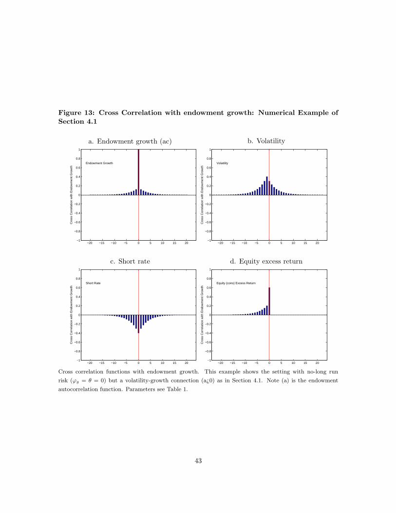
Figure 13: Cross Correlation with endowment growth: Numerical Example ofSection 4.1


−20 −15 −10 −5 0 5 10 15 20−1

−0.8

−0.6

−0.4

−0.2

0

0.2

0.4

0.6

0.8

1

Cro

ss C

orre

latio

n w

ith E

ndow

men

t Gro

wth

Endowment Growth

−20 −15 −10 −5 0 5 10 15 20−1

−0.8

−0.6

−0.4

−0.2

0

0.2

0.4

0.6

0.8

1

Cro

ss C

orre

latio

n w

ith E

ndow

men

t Gro

wth

Volatility


−20 −15 −10 −5 0 5 10 15 20−1

−0.8

−0.6

−0.4

−0.2

0

0.2

0.4

0.6

0.8

1

Cro

ss C

orre

latio

n w

ith E

ndow

men

t Gro

wth

Short Rate

−20 −15 −10 −5 0 5 10 15 20−1

−0.8

−0.6

−0.4

−0.2

0

0.2

0.4

0.6

0.8

1

Cro

ss C

orre

latio

n w

ith E

ndow

men

t Gro

wth


Cross correlation functions with endowment growth. This example shows the setting with no-long run

risk (ϕg = θ = 0) but a volatility-growth connection (a¿0) as in Section 4.1. Note (a) is the endowment

autocorrelation function. Parameters see Table 1.

43

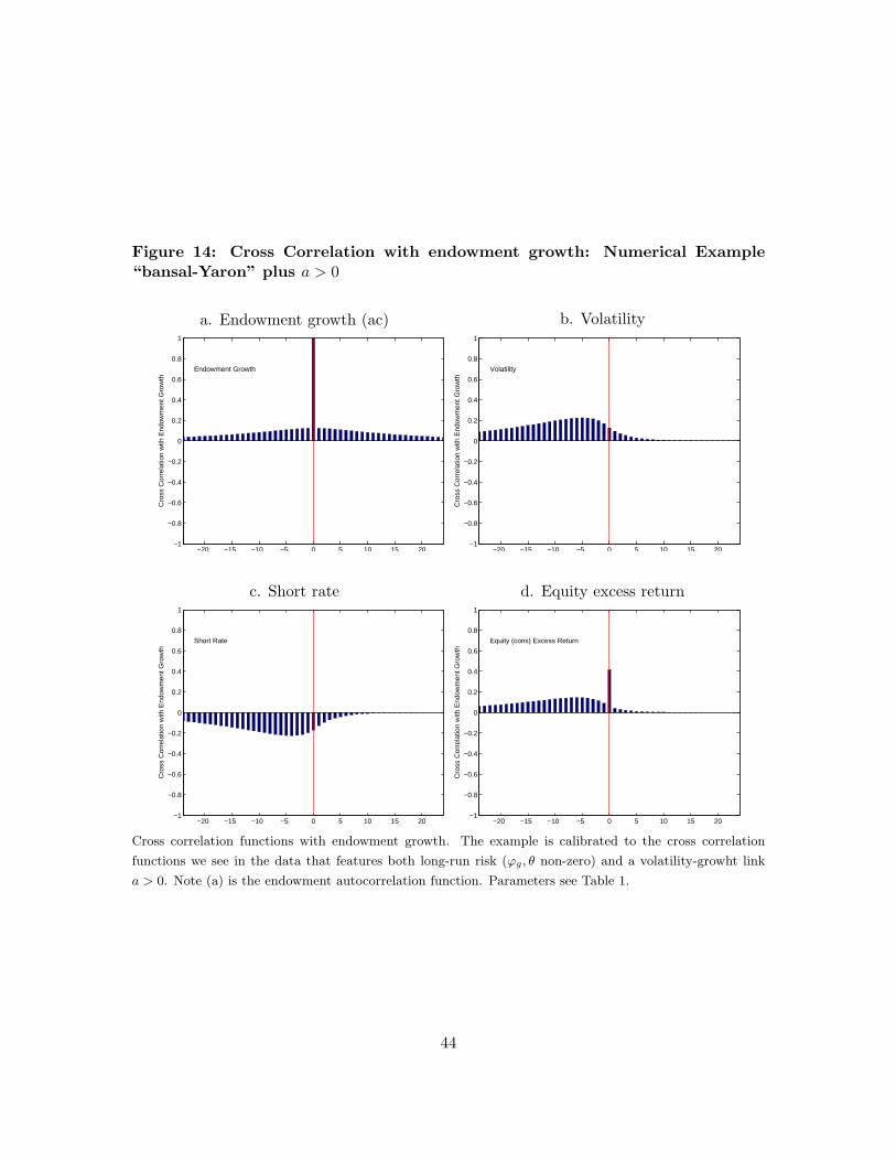
Figure 14: Cross Correlation with endowment growth: Numerical Example“bansal-Yaron” plus a > 0


−20 −15 −10 −5 0 5 10 15 20−1

−0.8

−0.6

−0.4

−0.2

0

0.2

0.4

0.6

0.8

1

Cro

ss C

orre

latio

n w

ith E

ndow

men

t Gro

wth

Endowment Growth

−20 −15 −10 −5 0 5 10 15 20−1

−0.8

−0.6

−0.4

−0.2

0

0.2

0.4

0.6

0.8

1

Cro

ss C

orre

latio

n w

ith E

ndow

men

t Gro

wth

Volatility


−20 −15 −10 −5 0 5 10 15 20−1

−0.8

−0.6

−0.4

−0.2

0

0.2

0.4

0.6

0.8

1

Cro

ss C

orre

latio

n w

ith E

ndow

men

t Gro

wth

Short Rate

−20 −15 −10 −5 0 5 10 15 20−1

−0.8

−0.6

−0.4

−0.2

0

0.2

0.4

0.6

0.8

1

Cro

ss C

orre

latio

n w

ith E

ndow

men

t Gro

wth


Cross correlation functions with endowment growth. The example is calibrated to the cross correlation

functions we see in the data that features both long-run risk (ϕg, θ non-zero) and a volatility-growht link

a > 0. Note (a) is the endowment autocorrelation function. Parameters see Table 1.

44

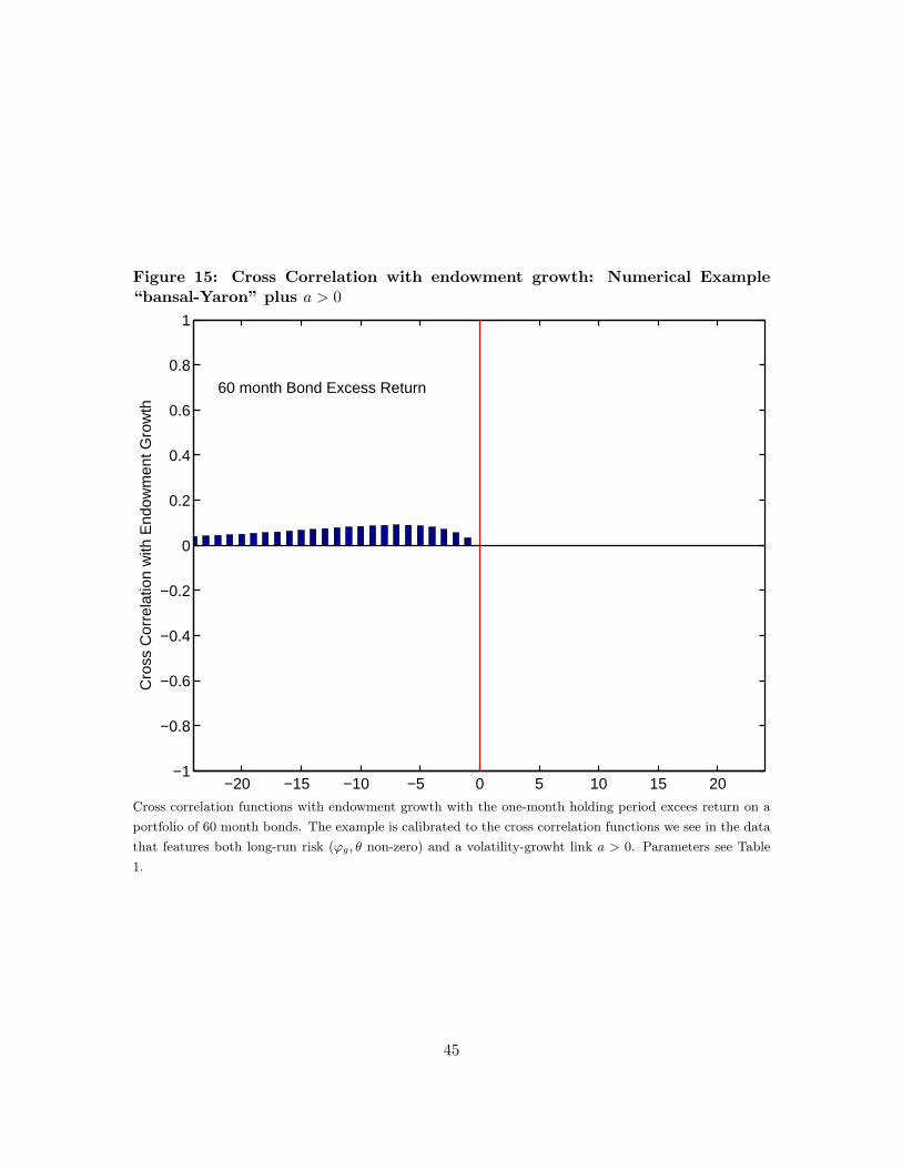
Figure 15: Cross Correlation with endowment growth: Numerical Example“bansal-Yaron” plus a > 0

−20 −15 −10 −5 0 5 10 15 20−1

−0.8

−0.6

−0.4

−0.2

0

0.2

0.4

0.6

0.8

1

Cro

ss C

orre

latio

n w

ith E

ndow

men

t Gro

wth

60 month Bond Excess Return

Cross correlation functions with endowment growth with the one-month holding period excees return on a

portfolio of 60 month bonds. The example is calibrated to the cross correlation functions we see in the data

that features both long-run risk (ϕg, θ non-zero) and a volatility-growht link a > 0. Parameters see Table

1.

45

the cyclical component of us asset...

Documents