The Costs of Financial Mistakes:

Evidence from U.S. Consumers∗

Adam T. Jørring †

Click here for most recent version

January 16, 2018

Abstract

This paper investigates the relationship between financial mistakes and lack of con-sumption smoothing, using transaction-level data from a million U.S. consumers. I firstdocument that, even in my sample of relatively sophisticated consumers, simple andavoidable card fees are pervasive and persistent. Avoidable fees correlate with loweraccount optimization, lower participation in risky asset markets, and lower mortgage refi-nancing. I measure the marginal propensity to consume using an event study of mortgagepayment resets and a difference-in-differences methodology. Consumers with a historyof frequent financial mistakes display low consumption smoothing out of predictable in-creases in debt payments, counter to models with rational borrowing constraints. Guidedby these results, I compare different economic mechanisms that link financial mistakesand lack of consumption smoothing: the evidence is more supportive of financial igno-rance rather than rational information inattention. A calibrated model of financial igno-rance indicates that for the 10% of consumers who make the most mistakes, the welfareloss amounts to $1,740 per year, equivalent to 8% of median annual non-durable con-sumption.

∗I am very grateful to my advisors Amit Seru, Amir Sufi, Lars Peter Hansen, and Gregor Matvos for guid-ance, support, and countless conversations throughout my PhD. I also thank Xavier Gabaix, Neale Mahoney,and Lawrence Schmidt for comments that substantially improved the paper. I also thank Simcha Barkai, JohnCochrane, Doug Diamond, Peter Ganong, Daniel Green, Menaka Hampole, Erik Hurst, Paymon Khorrami, Ste-fan Nagel, Pascal Noel, Raghuram Rajan, Willem van Vliet, Tony Zhang, and Luigi Zingales, as well as seminarparticipants at University of Chicago, University of Michigan, University of Texas at Austin, Harvard University,Stanford University, Boston College, Yale University, Rice University, and at the Summer 2017 Macro-FinancialModeling Conference for helpful comments. I gratefully acknowledge funding from the MFM Group and theBecker Friedman Institute. All errors are my own.†University of Chicago. Email: ajorring@chicagobooth.edu. Website: www.adamjorring.com.

1

"A year before the housing meltdown, Richard Peterson took out a $167,000 credit line on hisHuntington Beach condo. ... Peterson, 62, who has since retired, received his unpleasant shocklast month. ... (H)is payment will rise to more than $1,100 a month from the $400 he is payingto cover just the interest. ’We both now live on a fixed income and will not be able to make thepayments,’ he said of himself and his girlfriend."

LA Times, 8/7/2014: "Home equity line defaults are likely to rise".

1 Introduction

Why don’t consumers smooth consumption? A central finding in macroeconomics andfinance is consumers display a significant consumption response to predictable changes inincome, counter to the canonical life-cycle/permanent-income hypothesis (LC/PIH), withthe strongest effect concentrated among consumers with low liquidity.1 Understanding whatdrives lack of consumption smoothing is critical both for theoretical evaluations of models ofconsumption, as well as for empirical estimations of the macroeconomic effects of fiscal andmonetary policy.2

Research presents two contrasting views on what causes low liquidity and lack of con-sumption smoothing. The long-held conventional view is consumers have homogeneouspreferences and rational expectations. According to this view, lack of consumption smooth-ing and low liquidity is a consequence of idiosyncratic and uninsurable income shocks andrational liquidity management. For example, both the textbook buffer-stock models, as wellas recent models with multiple assets, predict that a high marginal propensity to consume(MPC) out of predictable income is situational and caused purely by temporarily low liq-uidity. However, according to the alternative view, low liquidity and lack of consumptionsmoothing are due to persistent differences in behavioral characteristics. These differencesmay include, for example, the degree of impatience, differences in attention to information, or– as I will argue in this paper – differences in consumers’ ability to make financial decisionsand financial plans.3

1A large body of empirical literature, going back at least to Zeldes (1989), has documented a high marginalpropensity to consume (MPC) out of predictable changes in income. Recent papers have studied the response tosocial security tax withholdings (Parker, 1999), income tax refunds (Souleles, 1999; Johnson, Parker and Souleles,2006; Parker, 2015), paycheck receipts (Stephens, 2006), and predictable decreases in loan payments (Stephens,2008; Di Maggio et al., n.d.). See the literature review for additional papers, and see Jappelli and Pistaferri (2010)for a recent survey.

2For example, MPC estimates from Johnson, Parker and Souleles (2006) are cited prominently by the Congres-sional Budget Office and the Council of Economic Advisers in their evaluation of the fiscal stimulus followingthe financial crisis (CBO, 2009; CEA, 2010). Additionally, recent work by Auclert (2016) and Wong (2015) arguethat differences in MPCs have a first-order impact on the effectiveness of monetary policy.

3The seminal papers on the conventional view of household consumption under incomplete markets includeBewley (1977), Deaton (1991), Huggett (1993), Aiyagari (1994), and Carroll (1997), and recent papers building onthese include Kaplan and Violante (2014) and Kaplan, Moll and Violante (2016). Research on the alternative viewincludes Mankiw and Campbell (1989), Caballero (1995), Lusardi (1999), Hurst (2003), and Reis (2006). See Parker(2015) for a review of the two views on what drives lack of consumption smoothing.

2

In this paper, I provide empirical evidence in favor of the behavioral view. I proposeand test the hypothesis that lack of consumption smoothing reflects a persistent tendency tomake financial mistakes. We have theoretical reasons to believe poor financial planning canlead to lack of consumption smoothing.4 However, various empirical challenges complicateinvestigation of this hypothesis, and despite rigorous efforts, the effect of financial mistakeson consumption smoothing remains largely unknown. The empirical challenges include bothdata- and measurement-related challenges as well as difficulties in inferring causation dueto omitted variables. In this paper, I address these empirical challenges using a unique anddetailed database of both account and card transactions from U.S. consumers. I measurefinancial mistakes and use variation in predictable increases in debt payments to assess howthese mistakes relate to consumption smoothing. My tests allow me to compare differenteconomic mechanisms that link financial mistakes and lack of consumption smoothing. Ithen develop a calibrated model of financial ignorance to assess the welfare losses due tofinancial mistakes.

I start my empirical analysis by documenting that financial mistakes are pervasive andpersistent. I face a key empirical challenge when measuring financial mistakes. Becausecomprehensive micro data have been previously unavailable, disentangling financial mistakesfrom rational liquidity demands has been difficult in past work.5 I counter this problem byusing the unique merge of both daily deposit balances and daily card transactions.

I define a financial mistake, as a financial decision where an unambiguous optimal choiceexists, and where the consumer does not choose the optimal choice.6 In my benchmarkanalysis I analyze two unambiguous financial mistakes: incurring an avoidable late fee, andincurring an avoidable overdraft fee. Following Stango and Zinman (2009) and Scholnick,Massoud and Saunders (2013), I define a late fee as avoidable, if on the payment day, theconsumer had sufficient balances in his deposit account to cover both the minimum balanceand an average month of consumption expenditure. Similarly, I define an overdraft fee asavoidable, if on the day the expenditure occurred, the consumer had sufficient liquidity (indeposit accounts and on other cards) to cover both the purchase and an average month ofconsumption expenditure.

I show that even in my sample of relatively sophisticated consumers, more than two thirdsof consumers incur avoidable card fees. The cost of these mistakes can vary quite a bit, with

4Conceptually, many of the psychological mechanisms underpinning financial mistakes, such as optimiza-tion mistakes and lack of sophistication, are also prevalent among consumers who display lack of consumptionsmoothing (Parker, 2015).

5Telyukova (2013) argues that the coexistence of high interest rate credit card debt and low interest-bearingdeposits can be rationalized by expenses that can only be paid in cash.

6The literature on household finance has identified numerous consumer choices that are hard to rationalizeusing models of optimal choice (see Campbell (2016)). These choices include both extreme decisions, with un-ambiguously optimal choices, and more complex decisions where the optimal choice is potentially sensitive toindividual consumer circumstances. The former unambiguous choices include, for example, incurring avoidableoverdraft fees, and the latter more complex choices include, for example, lack of mortgage refinancing.

3

around 20% of the consumers incurring mistakes that result in fees that range between $200and $950 annually.7 These fees are also persistent over time. For example, the probability ofincurring an avoidable late fee is only 22% if one didn’t incur any avoidable late fees in theprevious year. However, the probability of incurring an avoidable late fee increases to 64% ifone incurred at least one late fee in the previous year, and the probability increases to 92% ifthe consumer ranked in the top decile based on avoidable fees in the previous year.

My second and main empirical finding is consumers who frequently make financial mis-takes also display a lack of consumption smoothing. The main empirical challenge here isthat consumers who make financial mistakes often have low and uncertain incomes, and fewor no financial assets, and thus they are often borrowing constrained. Therefore, inferringwhether lack of consumption smoothing is the result of rational borrowing constraints orirrational financial mistakes is difficult. I address this challenge by using a predetermined,negative change in disposable income. Even a liquidity-constrained consumer - presumingsome degree of rationality - will save for predictable negative income changes. This asym-metry in the borrowing constraint, noted by Zeldes (1989), offers a concise method to isolatewhether the relationship one finds might be beyond rational borrowing constraints.8

In my analysis I use a predictable increase in the monthly mortgage payments for con-sumers who have taken out interest-only home equity lines of credit (IO-HELOCs). Aftera predetermined draw period, IO-HELOCs convert from open-ended interest-only loans, toclose-ended amortizing loans. This institutional design ensures borrowers face a sharp dis-continuity in their monthly payments after the draw period. The median monthly changein the sample is above $500 per month. It is worth emphasizing that despite the high stakesand the perfectly predictable reset date, anecdotal evidence suggests many consumers areunaware of the contractual features of their HELOCs. For instance, in a 2016 survey, TD Bankfound that more than one quarter of homeowners with HELOCs did not know when theirHELOC draw period end (TD Bank, 2016). Relatedly, only 19% knew the monthly paymentincreases when the draw period ends, and, surprisingly, 38% of those surveyed thought theirpayments would decrease.

My tests use an event study of predictable increases in debt payments employing a difference-in-differences research design. To implement this test, I sort consumers by their history ofmistakes at the end of the HELOC draw period. The "control" group are consumers who,up until the reset date, have never incurred any avoidable late or avoidable overdraft fees.

7It is worth noting that though the cost of the benchmark mistakes (avoidable late and overdraft fees) maybe relatively small (less than $100 per year for the median consumer), we study them because they unambigu-ously show that consumers differ in their ability to make financial decisions that might be quite costly. Theseinclude decisions such as lack of account optimization, lack of stock market participation, and lack of mortgagerefinancing.

8Jappelli and Pistaferri (2010) note in their review article that only a few empirical papers study income dropsother than retirement. Recent examples include Baker and Yannelis (2017) and Gelman et al. (2015), who examinethe spending response to loss of income following the federal government shutdown, and Ganong and Noel(2016), who study consumption around the expiration of unemployment benefits.

4

This group accounts for approximately 30% of the sample. I sort the remaining consumersin quartiles based on frequency of the two benchmark mistakes, measured just prior to thereset. The "treatment" group is the highest quartile, approximately 17% of the entire sample.

I show that the treatment and control group are similar, in terms of age, income, unem-ployment rate over past six months, and change in income over past six months. For example,the average income in the control group is $98,164 and $97,285 in the treatment group, and inboth groups the average unemployment rate in the past six months was 2%. The two groupsalso display similar credit scores. According to the bank’s internal credit score, the controlgroup had a score of 339 and the treatment group a score of 337 (out of 380). In addition,the two groups display similar consumption expenditure, prior to the reset date. The averagemonthly expenditure was $1,901 and $1,912 for the control and treatment group, respectively.The two groups are similar in the period before the event, not only on average but also periodby period.

A difference-in-differences research design reveals significant heterogeneity in the MPCacross measures of prior financial mistakes. For example, consumers with no history ofavoidable card fees smooth their consumption expenditure around the payment reset. Thisbehavior is in line with predictions from rational models. However, consumers with a historyof frequent mistakes cut their consumption expenditure by almost 9% following the paymentresets. Consumers cut their consumption across both durable and non-durable goods. Thelargest one-month cuts occur in the categories of travel (-$27), auto durables (-$26), healthcare(-$23), and restaurants (-$19). The difference in consumption sensitivity across the two groupsis robust to relaxing the threshold for what constitutes a financial mistake. For example, if wesort on all late and overdraft fees, not just avoidable fees, we see an even larger drop ($254).

Having established evidence in favor of behavioral view, when explaining the relationshipbetween financial mistakes and lack of consumption smoothing, the last part of my paper in-vestigates the economic mechanisms behind this link. I test two types of hypotheses: modelsof rational time constraints and models of financial ignorance. Using data on online andmobile logins, I find financial mistakes are positively correlated both with access to online ac-counts and with frequency of logins, even after controlling for age. This finding contradictsmodels in which time is the scarce resource preventing consumers from avoiding the fees.Next, I test whether financial mistakes are correlated with financial ignorance, as proxiedby measures of education. I use the shares of households in a ZIP who have completed atleast high school, 2-year college, and 4-year college, respectively, as proxies for the educa-tion of the consumers, and I find these proxies for education are negatively correlated withthe frequency of mistakes. For example, controlling for the income of the consumer, in ZIPcodes where many households have attained at least a 4-year college degree, the frequencyof mistakes is lower. Overall, these tests are more consistent with consumers with financialmistakes also being financially ignorant.

5

In the last part of my paper, I estimate welfare consequences of financial mistakes by cal-ibrating a consumption-savings model in which financial mistakes are the result of financialignorance. I micro-found the financial ignorance as a result of "cognitive sparsity" (Gabaix,2014, 2016b). This assumption of "cognitive sparsity" can both generate the per-period costof avoidable fees, as well as the lack of consumption smoothing around predictable debt-payment changes. Quantitatively, I calibrate the model to the HELOC expenditure profiles.I find that avoiding simple financial mistakes can save the median consumer $130 per yearand save the 10% of consumers with the most mistakes an average of $1,740 per year, whichis equivalent to 8% of median annual non-durable consumption.

Interestingly, the model generates an additional and testable qualitative implication: con-sumers are systematically wrong in their expectations of future liabilities from the interest-rate reset. That is, consumers who are ignorant of the contractual features of the HELOCwill under-estimate the value of future liabilities. In other words, ignorant consumers willbelieve they are wealthier than they are. I test this hypothesis by categorizing the type ofexpenditure into luxury and necessity, and by calculating Engel curves. I find that consumerswho frequently make mistakes have a higher expenditure ratio on luxury goods, especiallyfollowing increased credit limits.

My findings have both conceptual and practical implications. In terms of conceptual im-plications, my findings suggests differences in consumption smoothing can be attributed tofinancial ignorance, in a similar spirit to a nascent literature documenting that lack of con-sumption smoothing is related to persistent behavioral characteristics (Parker, 2015; Gelman,2017, 2016). The specific finding that mistakes correlate across multiple domains suggests thepsychological mechanism underpinning simple mistakes also distorts more complex deci-sions. In addition, my findings suggest the sparsity tools from statistical learning (Tibshirani,1996; Gabaix, 2014) are useful when modeling financial ignorance. Financially ignorant con-sumers can be modeled as assigning no attention to future interest-rate changes.

In terms of practical implications, my research adds to a growing empirical literature,measuring the welfare cost of financial mistakes (Agarwal et al., 2009; Calvet, Campbell andSodini, 2007; Lusardi and Tufano, 2015; Keys, Pope and Pope, 2016). Additionally, the bench-mark financial mistakes studied in this paper are simple and avoidable, and leave scope forfinancial products that "nudge" consumers (Thaler and Sunstein, 2008), for example, auto-payment systems to avoid credit card fees. However, the paper also finds that mistakes corre-late across multiple domains where "easy fixes" can prove insufficient, which leaves financialregulators with a difficult tradeoff when weighing the benefits of regulation to the consumerswho make mistakes against the costs of regulation to other financial market participants, asdiscussed by Campbell (2016).

6

Related literature

This paper builds on several related strands of literature in household finance, consump-tion theory, and behavioral economics. Within household finance, this paper contributes tothe literature on financial mistakes within credit and debit cards (Stango and Zinman, 2009,2014; Agarwal et al., 2009, 2013, 2015b,c; Scholnick, Massoud and Saunders, 2013; Gather-good et al., 2017; Ponce, Seira and Zamarripa, 2017). More broadly, this paper contributesto a growing literature on financial mistakes. This literature goes back at least to Bernheim(1995, 1998), who was among the first to show most households cannot perform very sim-ple calculations and lack basic financial knowledge. Subsequent empirical work includesresearch on mistakes within savings and investment (Madrian and Shea, 2001; Barber andOdean, 2004; Calvet, Campbell and Sodini, 2007; Choi, Laibson and Madrian, 2011), finan-cial literacy (Lusardi and Mitchell, 2007b,a; Lusardi and Tufano, 2015; van Rooij, Lusardi andAlessie, 2011b; Klapper, Lusardi and Panos, 2013), mistakes on mortgages (Andersen et al.,2015; Keys, Pope and Pope, 2016; Agarwal, Ben-David and Yao, 2017), and mistakes in adjust-ing to taxes (Chetty, Looney and Kroft, 2009; Finkelstein, 2009). Campbell (2016) is a recentsurvey of the literature on financial mistakes, and Lusardi and Mitchell (2014) offer a surveyof the literature on financial literacy.

A large theoretical literature investigates the determinants of consumption behavior. Theseminal work by Bewley (1977), Deaton (1991), Huggett (1993), Aiyagari (1994), and Carroll(1997) introduced the framework of consumption in incomplete market economies. Underthis framework, consumers smooth consumption from idiosyncratic and uninsurable incomeshocks subject to a borrowing constraint. In these models, the agent has rational expecta-tions and perfectly understands the impact of her financial decisions. With homogeneousconsumers, a high MPC is a rational consequence of the uninsurable income risk and a bor-rowing constraint. These models thus mark a departure from the classic PIH/LCI, whichpredicts a zero-consumption response to predictable changes in income. Many recent papershave highlighted the aggregate implications arising from heterogeneity in MPCs across thehousehold population (Eggertsson and Krugman, 2012; Kaplan and Violante, 2014; Guerrieriand Lorenzoni, 2015; Wong, 2015; Auclert, 2016; Greenwald, 2016). Two notable exceptionsthat depart from the assumption of perfect rationality are Gabaix (2016a) and Farhi and Wern-ing (2017). Both papers augment New Keynesian models with bounded rationality in theform of sparsity and level-k thinking, respectively. This paper contributes to the theoreticalliterature with empirical evidence on the empirical role of bounded rationality.

Concurrent with the theoretical literature, this paper also contributes to the empiricalliterature on consumer theory, which documents empirically that household consumptiondeparts from the standard LC/PIH model predictions. A large body of literature going backat least to Zeldes (1989) has studied the role of borrowing constraints on household con-sumption, and found consumption responds to predictable changes in income in a manner

7

suggesting the relevance of borrowing constraints. This literature includes studies of socialsecurity tax withholdings (Parker, 1999), income tax refunds (Souleles, 1999; Johnson, Parkerand Souleles, 2006; Parker, 2015), paycheck receipts (Stephens, 2006; Olafsson and Pagel,n.d.), job losses (Baker, 2017), and predictable decreases in loan payments (Stephens, 2008;Di Maggio et al., n.d.). However, a number of studies find no evidence in favor of borrowingconstraints (Hsieh, 2003; Coulibaly and Li, 2006). Recent studies that have found substantialheterogeneity in MPCs include studies of income shocks (Parker et al., 2013; Jappelli andPistaferri, 2014) and studies of MPCs out of shocks to housing prices and wealth (Mian andSufi, 2011; Mian, Rao and Sufi, 2013). The literature on consumption responses and borrow-ing constraints is also often used by policy makers to determine the effectiveness of monetaryand fiscal policy (CBO, 2009; CEA, 2010).

Similar to Baker (2017), Olafsson and Pagel (n.d.) use data from a personal finance appfrom Iceland and find that many households display consumption responses around pay-check receipts. These findings are also hard to rationalize with standard liquidity constraints,as the authors simultaneously observe sufficient liquidity from bank accounts. Olafsson andPagel (n.d.) argue that these results are not driven by financial sophistication, proxying,among other things, with age and number of logins. However, in this paper I find that bothage and number of logins are not linearly related to sophistication. I find that mistakes havea u-shaped relationship with financial mistakes and that the number of logins are positivelyrelated to the frequency of financial mistakes, and I find that the frequency of incurring finan-cial mistakes is negatively related to measures of education. In addition, my paper calibratesa model of financial ignorance and tests an out-of-sample prediction of financial ignorance:In line with the models predictions, I find that consumers who incur frequent financial mis-takes spend a higher fraction of their total consumption on luxury goods, such as travel,electronics, arts and jewelry.

The HELOC interest rate reset studied in this paper contributes to recent research whichhave studied the MPC out of negative changes in income. For example, Ganong and Noel(2016) study consumption around the expiration of unemployment benefits. They also find anegative consumption response, counter to rational models. Baker and Yannelis (2017) andGelman et al. (2015) examine the spending response to an unanticipated, temporary loss ofincome: the federal government shutdown.

Within behavioral economics, this paper contributes to the broad literature on market in-teractions between rational and non-rational agents: Akerlof and Yellen (1985); De Long et al.(1990); Tirole and Benabou (2003); DellaVigna and Malmendier (2004); Gabaix and Lalisbon(2006). For example, DellaVigna and Malmendier (2004) analyze the contract design of firmswhen consumers are time-inconsistent and partially naive. Among other markets – and re-lated to this paper – they analyze the market for credit card-financed consumption (a marketwith immediate benefits and delayed costs). They find credit card issuers will price above

8

marginal cost, introduce switching costs, and charge back-loaded fees. Another related pa-per is Vissing-Jørgensen (2012). Here the author uses detailed data from Mexico and showsthe type of purchase has predictive power for default. As in this paper, the author findsthat goods associated with high loss rates tend to be luxuries and tend to be purchased byindividuals who consume abnormally large fractions of luxuries given their income.

Outline

The rest of the paper is structured as follows. Section 2 covers the institutional backgroundand describes the data. Section 3 calculates the frequency of avoidable card fees and testswhether such fees are valid measures of financial mistakes. In section 4, I analyze the impactof financial mistakes on consumption smoothing. In section 5, I compare theories of financialmistakes and calibrate a model of financial ignorance, and section 6 concludes.

2 Background and Data

In this section, I describe the institutional background and data sources used in the em-pirical analysis. The empirical design relies on contractual details of credit and debit cardfees and the repayment structure of the HELOC. Fist, I describe the landscape of U.S. creditand debit card fees and describe the two fees I will use in the benchmark analysis: the latefee and the overdraft fee. I then describe the HELOC. Lastly, I present the specific data setused in the paper, built in collaboration with a large U.S. financial institution.

In my benchmark analysis, I measure the frequency of avoidable late and overdraft fees.As I will show below, both late and overdraft are common. The majority of U.S. banks imposeboth late and overdraft fees, and a large fraction of the population have incurred at least onethese fees.

2.1 Consumer banking and card fees

Credit and debit cards function as a method of payment and as a source of unsecuredconsumer credit for a large part of the U.S. population. According to the U.S. Census Bu-reau, 160 million card holders held more than a billion credit cards in 2012. The financialinstitutions that issue credit and debit cards earn an income on the cards – generally speak-ing – through two different sources: interest income and fees. Interest is earned on unpaidconsumer debt, and fees are levied partly on the consumers and partly on the merchants asa transaction fee. In aggregate, the income for U.S. financial institutions from credit card feeshave long surpassed income from interest on credit card debt (see figure A1).

The most common fees imposed on consumers from credit cards include annual fees,balance-transfer fees, cash advance fees, foreign transaction fees, over-the-limit fees, late, and

9

returned check fees. Common debit card fees imposed on consumers include annual ormonthly fees, atm fees, and overdraft and not-sufficient-funds (NSF) fees. According to theCFPB, revenues from consumer overdraft and NSF fees totaled $11.16B in 2015.

In this paper, I use data on two of the most common fees: the late fee, which is imposedon missing credit card payments, and the overdraft fee imposed on debit card transactionswith insufficient funds. Both the late fee and the overdraft fee are common in the UnitedStates: According to a survey by creditcards.com, 99 out of 100 general-purpose credit cardsimpose a late fee, with an average late fee of $37.9 According to a survey by nerdwallet.comof 30 U.S. financial institutions, all 30 charge an overdraft fee.10 Among credit card fees,other common fees include cash-advance fees (98 out of the 100 cards surveyed), returned-payment fees (77/100), balance-transfer fees (77 out of 89 cards that allowed balance transfersin 2016), and foreign-transaction fees (61/100). Only 25 and 6 of the cards surveyed imposedan annual fee and an overlimit fee, respectively.

The Credit Card Accountability Responsibility and Disclosure (CARD) Act of 2009 cappedthe size of late fees at $25 for the first instance and $35 for each additional late payment withinsix months. However, under the CARD act, the limits are subject to an annual adjustmentbased on a federal consumer price index, and the maximum late fee has been adjusted to$38 in 2017 by the CFPB. If a consumer goes six months without another late payment, theaccount resets to the lower first-time fee.

On top of the direct cost through the fee, a late payment can also impose an indirect coston the consumer through a so-called penalty APR. The penalty APR is a higher interest ratethat is imposed if the consumer violates the terms of the contract. A common "trigger" ofthe penalty APR is a late payment or exceeding one’s credit limit. While the national averagecredit card APR for the first six months of 2017 was 15.5%,11 the median penalty APRs was29.99%. The CARD act also imposed restrictions on how and when financial institutionscan impose a penalty APR.12 The financial institution can impose a penalty APR on futurepurchases (i.e., not on the existing balance) for any reason – including a missed payment –once the account has been open for at least 12 months. If the interest rate that applies to futuretransactions is changed, the financial institution is required to notify the consumer 45 daysin advance, specifying the reason for the rate increase, and the rate increase can only applyto purchases made 14 days after the notice was sent. Additionally, a financial institution canonly increase the interest rate on an existing balance if the customer is 60 days delinquent

9See http://www.creditcards.com/credit-card-news/2016-card-fee-survey.php (accessed on8/16/2017).

10See https://www.nerdwallet.com/blog/banking/overdraft-fees-what-banks-charge/ (accessed on8/16/2017).

11According to CreditCards.com’s monthly report: http://www.creditcards.com/credit-card-news/interest-rate-report-81617-up-2121.php

12Agarwal et al. (2015c) study the effect of the CARD act, and find that regulatory limits on credit card feesreduced overall borrowing costs with no evidence of an offsetting increase in interest charges or a reduction inthe volume of credit. Taken together, they estimate the CARD Act saved consumers $11.9 billion a year.

10

on making a minimum payment. Finally, the credit card issuer is required to terminate thepenalty APR after no more than six months after the date it was imposed, if the consumerhas paid all the minimum payments during that period.

In table A1 in the appendix, I have tabulated the average fee costs from six leading U.S.financial institutions for late fees, overdraft fees, and penalty APRs.

2.2 Home equity lines of credit

In my main empirical analysis, I measure the MPC out of a predictable and negativechange in disposable income. I use a specific contractual detail from a mortgage productcalled a home equity line of credit (HELOC), to generate this event study. A HELOC is acredit line given to a homeowner and for which the residence is used as security. Whenissuing a HELOC, the lender provides a line of credit up to a maximum draw amount, forexample, $50,000 or $100,000. The consumer can draw on the HELOC using either a speciallyissued credit card, writing a check, or in other ways.

Most HELOCs are structured with a draw period and a repayment period. During the drawperiod, which usually lasts 5, 10, or 20 years, the HELOC is an open-ended non-amortizingline of credit, which means the consumer is only required to pay interest on the outstandingprincipal balance. After the draw period ends and the repayment period begins, the HELOCconverts to a close-ended, amortizing loan. During the repayment period, the borrower mustpay down the principal by making payments equal to the balance at the end of the drawperiod divided by the number of months in the repayment period. Most repayment periodslast 10 to 20 years; however, some HELOCs are structured with a single full prepayment of theprincipal at the end of the draw period through a so-called "balloon" payment, at which pointmost borrowers refinance the loan. Johnson and Sarama (2015) study data from the FRY-14Mregulatory report and the CoreLogic Loan Performance Home Equity Servicing data, andthey find HELOCs with balloon payments are more prevalent among riskier households withlow FICO scores and high cumulative loan-to-value ratios (CLTV). To avoid this selection bias,I exclude all HELOCs with baloon payments from my sample.

Many HELOCs were issued in the early and mid 2000s, and many of the outstandingHELOCs converts in the mid to late 2010s. As macroeconomic conditions, in particular houseprices, improved following the crisis, the aggregate losses on HELOCs have been muted. Notethat since the financial crisis, many financial institutions have changed parts of their HELOCproduct features, for example, some HELOCs issued in 2017 require partial amortization inthe years leading up to the interest rate reset, and several financial institutions have begunactively reaching out to their consumers and reminding them of the upcoming payment reset.

Johnson and Sarama (2015) document an increased default risk following the conversion,and the increased risk has also been cited in the financial press.13 An article in the LA Times

13Rieker (2014); Gittelsohn (2013); Jurow (2016).

11

(Khouri and Scott, 2014) features a borrower who appears surprised by the loan conversion(emphasis mine):

"A year before the housing meltdown, Richard Peterson took out a $167,000 creditline on his Huntington Beach condo. ... Peterson, 62, who has since retired, re-ceived his unpleasant shock last month in a letter from Specialized Loan Servicing,the company that collects his mortgage payment. As of July 2016, his paymentwill rise to more than $1,100 a month from the $400 he is paying to cover just theinterest. "We both now live on a fixed income and will not be able to make thepayments," he said of himself and his girlfriend."

This paper complements Johnson and Sarama (2015) by analyzing how customers whohave a history of financial mistakes appear surprised like Mr. Peterson: I find that customerswith a history of financial mistakes (measured as the frequency of avoidable card fees) havea higher delinquency rate following the loan conversion.

2.3 Description of bank data

In collaboration with a large U.S. financial institution I have created a data set that allowsme to jointly study financial choices and expenditure choices. The data are solely from thisinstitution, which I will refer to as "my bank," and the data set is de-identified. The dataset is constructed using consumer data from 2012 to 2017. It includes transaction-level datafrom checking and savings accounts, credit and debit card transactions, data on mortgageacccounts, and estimates of total asset holdings. For my main analysis, I restrict my sampleto "active" consumers. My bank defines an active consumer as a consumer who has hadat least five monthly deposit-account outflows at some point. I further restrict the sampleto only consider consumers who also have at least one active credit card with the bank.An active credit card is defined as a card that at some point has had at least five monthlytransactions. From these two restrictions, I draw a random sample of 1 million consumers.Hence, I am analyzing a sample of 1 million bank customers who have both an active depositaccount and an active credit card with the same institution. Additionally, for the analysis ofMPC differences, I construct a sample of consumers with both an active deposit account andan active credit card and who hold a HELOC. This second sample has 320,000 consumers.

For each consumer, the data set includes a number of daily and monthly observations.The daily observations from the financial institution include transactions from credit anddebit cards and transactions from checking and savings accounts. Monthly data from the in-stitution include balances and interest rates from checking and savings accounts, the internalbank credit score, and the institutions own monthly estimates of total asset holdings. For theconsumers who hold a HELOC, the data set also includes additional variables related to their

12

HELOC. The HELOC variables are updated at a monthly frequency and the include originalbalance, credit line, interest rate, outstanding balance, and debt payments.

The main variables of interest are spending, income, assets, and liabilities. Below, I de-scribe how I construct each of these four variables. I construct the measure of spending,which captures 50% of all outflows from checking accounts from three components. The firstcomponent is debit and credit card spending, where I classify the month of credit card spend-ing as the month in which the expenditure occurs, not the month in which the credit card billis paid. The second component is cash withdrawals, and the third is bill payments. The other50% of outflows are made up of consumer debt payments, transfers to external accounts, anduncategorized outflows. The second main variable is income. I construct income from twocomponents that jointly make up 60% of inflows: (1) payroll paid using direct deposits and(2) government income. The remaining inflow categories include transfers from savings andinvestment accounts, other income, and uncategorized inflows. I use two measures of assets:total assets and liquid assets. My bank has a measure of total assets based on an internal sta-tistical model, which uses a combination of checking-account activity, transfers to investmentaccounts, and third-party data sources. The measure of liquid assets is constructed from bal-ances on savings and checking accounts within the bank. Finally, I construct a measure ofliabilities, using outstanding revolving balances on credit cards within the bank. The unit ofobservation for all five variables is consumer-by-month, from November 2012 through June2017.

3 Financial Mistakes

The literature on household finance has identified numerous consumer choices that arehard to rationalize using models of optimal choice (see Campbell (2016)). These choices in-clude both extreme decisions, with unambiguously optimal choices, and more complex deci-sions where the optimal choice is potentially sensitive to individual consumer circumstances.The former unambiguous choices include, for example, incurring avoidable overdraft fees,and the latter more complex choices include, for example, lack of mortgage refinancing.

In this paper, I define a financial mistake, as a financial decision where an unambiguousoptimal choice exists, and where the optimal choice is not chosen by the consumer. In mybenchmark analysis I analyze two unambiguous financial mistakes: incurring an avoidablelate fee, and incurring an avoidable overdraft fee. Following Stango and Zinman (2009) andScholnick, Massoud and Saunders (2013), I define a late fee as avoidable, if on the paymentday, the consumer had sufficient balances in his deposit account to cover both the minimumbalance and an average month of consumption expenditure. Similarly, I define an overdraftfee as avoidable, if on the day the expenditure occurred, the consumer had sufficient liquidity(in deposit accounts and on other cards) to cover both the purchase and an average month of

13

consumption expenditure.Given this definition of a financial mistake, I show that even in a sample of relatively

sophisticated consumers, financial mistakes are pervasive – more than two thirds of con-sumers incur avoidable card fees – and persistent. For example, the probability of incurringan avoidable late fee is only 22% if one didn’t incur any avoidable late fees in the previousyear. However, the probability of incurring an avoidable late fee increases to 64% if one in-curred at least one late fee in the previous year, and the probability increases to 92% if theconsumer ranked in the top decile based on avoidable fees in the previous year.

In the last part of this section, I document that these simple financial mistakes correlatewith more complex – and more expensive – financial decisions, such as lack of account opti-mization, non-participation in stock markets, and lack of mortgage refinancing. This findingsuggests that the latter more costly decisions are also distorted by optimization failures.

Combined, these results act as validity tests in favor of the notion that avoidable fees area good proxy for poor financial decisions.

3.1 Measure of financial mistakes

An overdraft fee is a fee that is levied when a withdrawal exceeds the available balance.If the consumer makes a purchase using a debit card that is linked to an account with in-sufficient funds, an overdraft fee is levied on the account.14 A late fee is a fee levied oncredit card delinquency (i.e., failure to pay at least the minimum balance on the due date).I follow Scholnick, Massoud and Saunders (2013), and classify a fee as an avoidable fee ifthe consumer incurred the fee while simultaneous holding sufficient liquidity to meet eitherthe purchase or minimum balance, respectively. In the case of an overdraft fee, I classify anoverdraft fee as an avoidable fee if.

Expenditure < Balances on deposit accounts + Card liquidity − 1 month spending(3.1)

And I classify a late fee as avoidable if,

Minimum Payment Due < Balances on deposit accounts− 1 month spending (3.2)

where one-month spending is estimated as the average monthly outflow. Note the right-handside of equation 3.1 includes liquidity broadly defined, that is, both account deposits as wellas available unused credit limits on different cards, whereas the right-hand side of equation3.2 only includes account deposits. Scholnick, Massoud and Saunders (2013) identify twokey reasons for subtracting precautionary balances: (1) consumers might fear being liquidity

14In general, overdraft fees are ascribed to all deposit transaction with insufficient funds. However, in thispaper, I only analyze overdraft fees occurring from debit card purchases. That is, I am not classifying overdraftfees from other types of deposit account transfers as avoidable fees.

14

constrained in the future and/or (2) consumers are currently liquidity constrained.The direct cost of incurring an overdraft fee is the overdraft fee itself:

φoverdraft = overdraft fee. (3.3)

The late fee includes an additional term. As described in Table A1, some credit cards have anassociated penalty APR. Conditional on credit card delinquency, the APR on the credit cardincreases to the penalty APR. Thus, the cost of not paying at least the minimum balance is

φlate = late fee + ∆APR×Average Daily Balance. (3.4)

3.1.1 Results

In figure 1 I report the average annual costs of incurring avoidable late payment fees andoverdraft fees. The average costs is calculated from 2012 to 2016 both inclusive. Customersare sorted by average yearly frequency of number of financial mistakes, and we see that alittle less than one third of the population never incurred either an avoidable late fee or anavoidable overdraft fee in the five year period. Another third incurred less than one avoidablefee per year across the five years. The next 20% of the consumers incurred on average betweenone and three avoidable fees per year at an average yearly cost of around $75. The next 9%of the consumers incurred between three and six fees per year at an annual cost of $200. Thenext 4% incurred between 6 and 10 avoidable fees at a yearly cost of $350, and the last 5% ofthe consumers incurred more than 10 fees per year, i.e. more than 50 avoidable fees acrossthe five year period. And the cost of these more than 50 avoidable fees were a yearly averageof more than $950.

Combined, these results indicate that unambiguous are pervasive, more than two-thirdsincur them, however the majority of the direct costs of financial mistakes are born by a smallerfraction of the population.

[Figure 1 about here.]

3.1.2 Demographic and financial characteristics

In table 1 I report demographic and financial characteristics of consumers sorted by thefrequency of avoidable fees. The first column represents the 31% of consumers who in theperiod from 2012-2016 incurred neither an avoidable late payment fee nor an avoidable over-draft fee. The next four columns are sorted in quartiles by frequency of avoidable fees.

[Table 1 about here.]

We see that consumers with no fees are slightly older, but that there is no relationshipacross age conditional on a single mistake. Although there is no linear relationship with age,

15

I do find a systematic non-linear relationship. Similar to Agarwal et al. (2009) I find a u-shaped life-cycle pattern across age. In figure 2 below I report the fitted value in a predictiveregression of frequency of mistakes on age dummies and deciles of controls (income, creditscore, and liquid assets), computing the intercept using the sample means for the controls.Agarwal et al. (2009) suggests that this u-shaped relationship reflects learning among theyoung and dementia or lower of IT literacy among the elderly15.

[Figure 2 about here.]

There is a light variation across groups on annual income; the annual income of con-sumers with zero avoidable fees is $72k while the average annual income among the quartilesare between $73 and $63, falling in frequency of mistakes. There is however a significant vari-ation across both total and liquid asset holdings. Both total and liquid assets increase from$148k and $7k to $367k and $24k respectively when comparing consumers with the mostamount of avoidable fees with those without any. Credit card limit utilization increases infrequency of fees, while debt-to-income ratios are fairly stable. The percentage of consumerswho have an online or mobile account is increasing in frequency of avoidable fees, and so aremedian monthly logins (conditional on having an account).

It is worth noting that although income does not seem to vary across the financial mis-takes bin, total assets do. This suggests that our measure of financial mistakes proxies forbehavior which leads to consumption inequality beyond income inequality (Campbell, 2016).For example, as consumers who make financial mistakes also have a lower savings-rate, theiraccumulated lifetime wealth is lower than the consumers who rarely make financial mis-takes. This suggests that improving financial literacy could have significant effects on wealthinequality, a point raised by Lusardi and Mitchell (2007a).

3.2 Validity of measure

In the previous section I outlined the data and measured the frequency of avoidableoverdraft fees and avoidable late fees. I this section I outline a number of validity tests. Thepurpose of the tests is to assess to what extend the avoidable card fees are a good measure offinancial ignorance. I analyze to what extent the frequency of these avoidable overdraft feesand late payment fees is a valid measure of financial mistakes. The purpose is to test to whatextent avoidable fees are indeed financial mistakes.

3.2.1 Calculating the implied discount rate

I estimate the implicit discount rate which the consumers are paying. If consumers areperfectly rational, they will only pay the avoidable fees, if they value their liquidity at at least

15I thank Virginia Traweek for drawing my attention to anosognosia, the phenomenon in which seniors whohave dementia tend to not fully recognize the extent of their impairment.

16

that discount rate. I follow the standard methodology for calculating annual percentage rateon consumer debt:

APR =Interest Charges

Average Daily Balance× 365

Days in Billing Cycle(3.5)

And equivalently for the overdraft mistake and the late payment mistake respectively I cal-culate:

Implied discount rate =Cost of ODMExpenditure

× 365Days in Billing Cycle

(3.6)

Implied discount rate =Cost of LPM

Minimum balance× 365

Days in Billing Cycle(3.7)

In figure 3 I report histograms of the implied discount rates for the two mistakes.

[Figure 3 about here.]

The distribution of implied monthly discount rates for the overdraft mistake range fromalmost 0% (when the purchase is very large relative to the fee) to more than 700% (when thepurchase is small relative to the fee). The range of implied monthly discount rates for thelate payment mistakes start at 100% as the late fee is almost always larger than the minimumpayment itself.

As an illustrative example consider a consumer who has an outstanding balance of $1,000,with a minimum payment due of $25. Regular APR=18%, Penalty APR=29.99%, and LateFee=$35. He considers the following two options: a) Only pay the minimum balance of$25, and thus borrow $975 for one month, and b) Not pay anything: borrow $1,000 for onemonth. The cost of these two options after one month are as follows: a) Total Finance Charge= 18%/12*$975 = $14.63. b) Total Finance Charge = 29.99%/12*$1,035 + $35 = $60.87. We seethat the consumer will pay an additional $46 just to avoid paying the minimum payment of$25. That is equal to an implied a one-month interest rate of 185% (which is in line with thehistogram of implied discount rates, see figure 3.

In order for a model with rational expectations to accurately describe these financial mis-takes, the model must have preference parameters that allow the agent to pay monthly dis-count rates of above 100%.

3.2.2 Persistence of financial mistakes

In this section I analyze to what extend incurring an avoidable credit or debit card fee israndomly distributed across individuals, or to what extend it is a persistent characteristic ofthe consumer.

In the first step of this analysis, I run a linear predictive regressions, predicting whetherconsumer i will make at least a financial mistake of type j over the next 12 months, as a linear

17

function on both a dummy indicating whether the consumer made a mistake in the prior 12months as well as on the number of prior mistakes at time t and a non-parametric functionof controls:

1{mistakei,t→t+11} = β× 1{mistakei,t−12→t−1} + f (controlsit) + εit (3.8)

1{mistakei,j,t→t+12} = β×mistakei,j,t + f (characteristicsit) + εit (3.9)

The regression coefficients are reported in 3. The conditional probability of incurringan avoidable late fee over the next 12 months increase from 10% to more than 32% if theconsumer had incurred an avoidable late fee in the prior 12 months. Equivalently we seefrom regression 3.9 that for every avoidable late fee in the past 12 months, the probabilityincreases with 12%-points for the following 12 months period. Equivalently, previous avoid-able overdraft fees has a positive impact on the probability of future overdraft fees, a changein 15%-points for the dummy and 8% in the linear regression. The cross-correlations, regress-ing future late fees on past overdraft fees and vice versa, also have positive and statisticallysignificant coefficients, albeit the economic magnitudes are slightly smaller.

As a second step in this analysis, I estimate a linear probability regressions where thedependent variable is the presence of a financial mistake by consumer i in month t:

1{mistakeit} = f (characteristicsit) + µi + εit (3.10)

I use decile bins to non-parametrically control for: "Age", "Income", "Liquid assets", "To-tal assets", "Expenditure volatility", "credit score", "Debt-to-income", "Online account", and"Number of logins". As goodness-of-fit measures I calculate adjusted R2, the square root ofthe mean squared error (RMSE), the mean absolute error (MAE), and the Pearson Correlation.Table 3 reports the results. We see that the explained variation increases by including a per-son fixed effect, and that effect appears across all four measures of goodness-of-fit increase:Adjusted R2 and the Person Correlation increase, and the RMSE and MAE decrease.

[Table 2 about here.]

We can see the same result from a simple variance decomposition. I calculate the fractionof the variance of the dependent variable which can be explained by a personal fixed effect:

Var(Y) = Var(

E[Y|X

])︸ ︷︷ ︸

Explained/between group variance

+ E[Var

(Y|X

)]︸ ︷︷ ︸

Unexplained/within group variance

In appendix table A2 I calculate the variance decomposition the frequency and cost of thelate payment mistake and the overdraft mistake. And the explained variance is Var

(E[Y|X

])/Var(Y).

I find that price variation between the consumers explain between 25% and 35% of the vari-

18

ation. Given the unconditional probability, if the mistakes were distributed randomly, thena variance decomposition would should that the variation between customers would onlyexplain between 2% and 3% of the variation. These results indicate that financial mistakesare not driven by random liquidity shocks. Instead, the data suggests that financial mistakesare driven by a persistent characteristic, in line with the behavioral view.

So far I have analyzed how much of the cross-sectional variation can be explained bya person fixed effect. In a second set of regressions, I look at the time-series dimension toanalyze persistence across time. I regress a linear probability model of future mistakes attime t + j conditional on making a mistake at time t. I interact the effect with the numberof mistakes at t, to see how the conditional probability of future mistakes vary with theconsumer’s history of mistakes. Table 4 reports the regression coefficients. Consistent withthe result in Agarwal et al. (2009) we see a short-term reversal in the probability of a mistakeoccurring. However this ’learning’ effect almost completely dissipates when interacting with"repeat offenders". We see this as the coefficient on the interaction term larger and increasing.

[Table 3 about here.]

Lastly I calculate the transition probabilities across two two-year periods. I divide thesample into 2013-2014 and 2015-2016 and sort consumers by their quartile of financial mis-takes within each two-year period. I then calculate the transition probability of moving frombin i to bin j, Prij, as the fraction of consumers who were in bin i in 2013-2014 and in bin j in2015-2016. Appendix table A3 reports the transition probabilities, and we see that a lot of theprobability mass is centered on the diagonal.

3.2.3 Mistakes across multiple domains

In a second validity test, testing the validity of using avoidable fees as a proxy for financialignorance, I compare the avoidable card fees with other standard financial mistakes, and Ianalyze if mistakes are correlated across domains. If the avoidable card fees that I measureare in fact financial mistakes caused by limited financial knowledge, then this would implythat consumers who incur frequent avoidable card fees also will exhibit similar behavioracross other domains. In this section I measure four other types of financial mistakes andcalculate the cross-sectional correlation. The four mistakes include two account optimizationmistakes, lack of mortgage refinancing and stock market non-participation.

Following Gathergood et al. (2017) and Ponce, Seira and Zamarripa (2017), I calculate thecredit card payment mistake and the credit card spending mistake as follows: The optimalrule for allocating credit card payments is: (1) pay min. payment on all cards, then (2) payhighest APR card. If a consumer is not following this optimal rule, he incurs a cost of

φpayments =(

rhigh − rlow

)∗min

{(smthigh −minhigh), (pmtlow −minlow)

}(3.11)

19

Similarly the optimal rule for allocating credit card expenditure is to allocate the expenditureon the card with the lowest effective APR, and a cost is incurred when: (finance charges oncard i with spending) AND (card j 6= i has unused credit and lower effective APR). The costis measured as:

φspending =(

rhigh − rlow

)∗max

{chigh, limitlow

}(3.12)

While the above two optimization mistakes have relatively low costs for the consumer,there are examples in the literature of financial mistakes with much higher stakes. Oneparticular example is the lack of mortgage refinance Andersen et al. (2015); Keys, Pope andPope (2016); Agarwal, Ben-David and Yao (2017). Following this literature I define a "lackof mortgage refinancing" mistake by the following algorithm: credit score above 680, LTVbelow 90, and mortgage rate with the option to refinance above the average 30-year fixed rate+ 0.5%-point.

Another "large-stake" financial mistake documented in the literature is "Stock MarketNon-Participation" (Calvet, Campbell and Sodini, 2007; van Rooij, Lusardi and Alessie, 2011a;Klapper, Lusardi and Panos, 2013). I’ve merged the data on financial mistakes on creditand debit cards with data from investment accounts within the financial institution. And Icalculate the cross-sectional correlation between the card mistakes and non-participation ininvestment accounts.

[Table 4 about here.]

In table 5 I report the cross-correlations between the two benchmark mistakes and thecredit card payment, credit card spending mistake, failure to refinance a mortgage, and non-participation in investment accounts. Table 5 reports the correlation across bins of frequencyof avoidable late fees and table 6 reports across bins of frequency of avoidable overdraft fees.

When we compare the group of consumers who have never incurred an avoidable late feewith the highest quartile, we see that the conditional probability of incurring an avoidableoverdraft fee increases from 36% to 68%. Equivalently the probability of making a credit cardspending mistake increases from 74% to 82%; the probability of making a credit card paymentmistake increases from 54% to 66%; the probability of not refinancing your mortgage whenit is optimal to do so increases from 87% to 93%; and the fraction of customers without aninvestment account increases from 92% to 98%.

Equivalently, comparing the group of consumers who have never incurred an avoidableoverdraft fee with the highest quartile, we see that the conditional probability of incurringan avoidable late fee increases from 55% to 62%. The probability of making a credit cardspending mistake increases from 73% to 81%; the probability of making a credit card pay-ment mistake increases from 54% to 65%; the probability of not refinancing your mortgage

20

when it is optimal to do so increases from 88% to 92%; and the fraction of customers with-out an investment account increases from 93% to 98%. In appendix table A5 I report theunconditional frequency of each of the four card mistakes.

3.3 Discussion

In the above section I measured the frequency of two benchmark financial "mistakes":paying a late fee while having sufficient liquidity available and paying an overdraft fee whilehaving sufficient liquidity available. Both of these fees are avoidable, as sufficient liquidityis available on the on the due-day and the payment day respectively. And incurring both ofthese fees is a financial choice which differs from the simplest rational models.

I conducted a number of validity tests of avoidable fees as a measure of financial mistakes.First, I calculate the implicit discount rate paid by consumers who incur either the avoidablelate fee or the avoidable overdraft fee. These were reported in figure 3, and we see that forthe majority of the fees paid, the implicit monthly was higher than 100%, counter indeed tomost rational models. In a second validity test I find that the avoidable card fees are highlypersistent within an individual consumer, and in the last validity test I find that avoidablecard fees correlate with other choices that the literature have associated with sub-optimalfinancial behavior, such as lack of between account optimization, lack of mortgage refinance,and lack of stock market participation.

4 Financial Mistakes and Consumption Smoothing

In the previous section I described the two benchmark financial mistakes, the avoidablecredit card late fee and the avoidable debit card overdraft fee. I showed that these mistakesimply a high discount rate, persistent, and correlated with other mistakes. And I found sug-gestive evidence that they are caused by financial ignorance, rather than rational inattention.

In this section I investigate the effects of financial mistakes on consumption smoothing.In order to test the effect of financial mistakes on consumption smoothing I conduct an event-study. I study a subsample of consumers who have all taken a Home Equity Line of Credit(HELOC). Payment for the HELOC is structured across two time periods. In the first period,the draw period, which typically lasts five or ten years, the consumer is only required to makeinterest payments. The interest rate is often floating and pegged to the prime rate. After thedraw period the HELOC converts into a fully amortizing loan with a repayment period ofbetween 10 and 20 years.

Figure A3 in the appendix outlines an example of a payout profile of a HELOC. In thisexample a hypothetical consumer has borrowed $50,000 using a HELOC. For the first 10 yearsthe monthly payment during the draw period is $145.83, and thereafter the monthly paymentincreases to $494.43.

21

The sample of consumers who have a HELOC have incurred financial mistakes at approx-imately the same frequency as consumers in the full sample. We see this in 4 where I haveplotted the frequency of consumers incurring either the late payment mistake, the overdraftmistake or both, sorted on average annual cost for the period November 2012 to June 2017,and we see that the distributions are very similar.

[Figure 4 about here.]

4.1 HELOC event-study: empirical specification

In this section I analyze the effect of financial mistakes on consumption fluctuations. Therational buffer-stock models will predict a zero change in consumption from a predictablenegative, and I consider this the first null-hypothesis. In my first empirical test I calculateimplied consumption by reset date for the entire sample:

Yit = α + µi + νtime + βtResetit + ΓXit + ε it (4.1)

In figure I plot the fitted values of consumption relative to the reset date16. This figure plotsmonths relative to the HELOC reset on the x-axis (date 1 is the first month after the end ofthe Draw Period), and the fitted value of total consumption expenditure on the y-axis. Theexpected consumption is around $1,900 per month and slightly decreasing towards the endof the draw period; directly after the draw period ends, the consumption falls with more than$50 and it continues to fall over the next 6 months. This pattern is inconsistent with a rationalbuffer-stock model.

[Figure 5 about here.]

Given the average result, I will test whether consumers who have a history of financialmistakes are more likely to cut their consumption following the HELOC reset. This test re-lates to a prediction from the survey literature on financial literacy: From the survey evidence(e.g. Lusardi and Mitchell (2007b)) we see that consumers who display low levels of finan-cial literacy also appear to be "bad planners". I.e. the consumers who answer incorrectlyon questions regarding interest rates and compound interest also save less for retirement. Itest whether this feature also is present in my data. I conduct this test using a subsample ofconsumers who have taken out interest-only Home Equity Lines of Credit (IO HELOCs). IOHELOCs have the particularly feature that for the first 5 or 10 years of the loan, the borroweronly has to pay interest on the outstanding balance. This initial period is called the drawperiod. Following the draw period is a repayment period, often 20 to 25 years, over which theremainder of the loan is amortized.

16I use the methodology from Agarwal et al. (2013) to compute the intersect.

22

This institutional setup means that borrowers of IO HELOCs faces a sharpe discontinuityin their monthly payments after the draw period. (See appendix figure A3 for an example.)Johnson and Sarama (2015) also use this discontinuity in payments, and they study defaultrisk. They find that HELOCs have significantly higher default and payoff rates around theend of the draw period.

In order to test whether consumers who have a history of financial mistakes experiencea higher MPC out of a predictable negative shock to income, I first sort consumers by theirhistory of mistakes at the end of the draw period. The "control" group are the consumerswho up until the reset data has never incurred any avoidable late or avoidable overdraft fees.This group accounts for approximately 30% of the sample. Among the remaining consumers,I sort the consumers in quartiles based on frequency of the two benchmark mistakes, andthe "treatment" group is the highest quartile. In table 7 I report the mean value of Age,Income, Change in income over past six months, unemployment rate over past six months,internal credit score, total assets, liquid assets, and percentage of consumers who have aninvestment account. We see that for the variables on age and income the two groups aresimilar. However, for the remaining variables – those more related to financial choices – thetwo groups differ: The group who have made many mistakes have a lower (albeit still high)credit score. A significantly lower total assets and liquid assets, a higher debt-to-income, ahigher credit card utilization rate and a lower frequency of investment accounts.

[Table 5 about here.]

To compare the differential consumption response to HELOC resets between the twogroups, I run the following regression:

Yit = α + µi + νtime + β jtResetjit + ΓXit + ε it (4.2)

The dependent variable Yit is total expenditure which is calculated as "credit card expendi-ture"+"debit card expenditure"+"account outflows"-"account outflows to pay for card debt".Notice that the last term is to ensure that card payments are not double counted. Also notethat t indexes months relative to the HELOC reset date – not calendar time. Instead νtime

is the calendar month fixed effect. The parameter α is a constant, µi is a consumer fixedeffect. βt is a vector of coefficients multiplying Resetit, a set of monthly dummy variablesfor dates relative to HELOC reset. Γ is a matrix of coefficients multiplied on Xit which hasdeciles of the control variables mentioned above. I sort consumers by frequency of mistakesat HELOC-date=0, and then run regression 4.2 twice, once for the sample of consumers whohave zero mistakes at HELOC-date=0, and once for the consumers in quartile 4, measure atHELOC-date=0.

23

I also run a difference-in-difference analysis to calculate change in consumption expendi-ture for the treatment group of different expenditure groups. I run the following regression:

Yit = α + β11Loan age > reset dateit+ β21Ignoranti

+ β31Loan age > reset dateit× 1Ignoranti

+ ε (4.3)

The coefficient of interest the is coefficient on the interaction between the HELOC loanhaving reset and the treatment group of consumers. Below I report the coefficient for regres-sions where t = 12 months across a number of consumption categories.

4.2 HELOC Event-study: Results and robustness

Figure 6 plots the coefficients from βt from regression 4.2. The two groups of consumershave pre-trends that are similar both in trend and at a level of approximately $1,200 in creditcard expenditure per month. Following the HELOC reset, the "control-group" (the groupof consumers with no mistakes) experience no statistically significant change. The pointestimate falls sightly, between $0 and $10 over the following 24 months, however this iswithin the standard errors of roughly $50.

The treatment group, the consumers in the highest frequency-quartile of mistakes, on theother hand experience a significant decline in credit card expenditure. Following the HELOCreset, the fitted value of credit card expenditure for the the treatment group falls from around$1,200 to around $1,100, or almost 9%. We see that the decline is roughly linear from months0 to month 21 and that it plateaus out from months 21 to month 24. This fall is significant at5%-significance level.

[Figure 6 about here.]

We see that the point estimate on income is negative, however this fall is insignificant. Thelargest drops occurs in the categories of Travel (-$27), Auto durables (-$26), and Healthcare(-$23). However, in the categories of Department Stores and Entertainment the point estimateis positive ($19 and $21 respectively), although statistically insignificant.

As a robustness exercise, I follow the methodology in Mian and Sufi (2012) and conducta placebo analysis where I sort consumers at different HELOC-dates and plot the differencebetween the credit expenditure of the two groups. I have plotted the coefficients from threedifferent placebo starting dates in appendix figure A3, and we see that the consumption dropfollowing the HELOC reset is significantly outside the band of other placebo tests.

4.3 Discussion

A large previous empirical literature has studied the effect of borrowing constraints onconsumer MPCs using predictable and positive changes to disposable income (Parker, 1999,

24

2015; Souleles, 1999; Johnson, Parker and Souleles, 2006; Stephens, 2006, 2008; Di Maggioet al., n.d.). This paper runs a similar event-study that compares the MPC out of predictableincome changes across different groups of consumers. However, while the previous literaturehas studied predictable positive changes in disposable income, this paper studies a predictablenegative change in disposable income. This seemingly innocuous difference allows for asharply different interpretation.17

[Figure 7 about here.]

Figure 7 above represents a graphic explanation of this logic: With a predictable posi-tive increase in disposable income the regression can distinguish between the consumptionresponse from an unconstrained LC/PIH model from the consumption response of a con-strained household. However, with a positive change the regression cannot distinguish be-tween the consumption response of rational model and an ignorant model.

With a predictable negative change, the regression allows the econometrician to distinguishbetween a borrowing-constrained and rational agent from that of an ignorant agent. See figure8 below.

[Figure 8 about here.]

5 Mechanisms and Magnitudes

In the previous sections we found that financial mistakes are prevalent, and that con-sumers who often make financial mistakes on average smooth their consumption less acrossa predictable negative change in disposable income. We have hypothesized that this rela-tionship is driven by heterogeneity in consumer’s ability to make financial decisions. In thissection I discuss and test potential alternative mechanisms.

5.1 Are consumers busy?

One potential alternative mechanism is that consumers who pay avoidable card fees aresimply too busy. It is time consuming to pay your credit card bill on time and being up to datewith which card that has sufficient funds, and potentially some consumers just value theirtime higher than the cost of the fee. I will test this alternative theory by looking at proxies forthe cost of time and compare those with measures of the level of education. The first proxyfor the value of time is whether or not the consumers has access to an online account with

17Other recent research that study the MPC from negative changes in income include Ganong and Noel (2016)who study consumption around the expiration of unemployment benefits. They also find a negative consumptionresponse, counter to rational models. Baker and Yannelis (2017) and Gelman et al. (2015) examine the spendingresponse to an unanticipated, temporary loss of income: the federal government shutdown.

25

the bank. I find that among consumers who never have never incurred an avoidable card fee88% has an online account and 58% has a mobile account. Whereas among the quartile ofconsumers who have incurred the most avoidable fees, 92% have an online account and 70%has a mobile. Additionally, the median number of logins is higher for the group of consumerswho make many mistakes, 18 online and 12 mobile, versus a median of 13 online and 6 mobilelogins for the group of consumers who never make mistakes. One potential confoundingeffect is that older people on average tend to be less tech savy which could drive this effect.However, I find that even after controlling for age fixed effects, consumers who have an onlineaccount are 0.7% more likely to make a monthly mistake than consumers without one. Wesee this in table 8, where I report the regression coefficients of linear regressions of mistakefrequency on a dummy variable taking the value one if the consumer has an online account.In the regression I control for income and have age and month fixed effects. The same resultappears if we regress mistake frequency on number of logins as well – see regression (2).After controlling for age and income, the effect of one additional monthly login increases theprobability of a monthly mistake with .06.

[Table 6 about here.]

In a second set of regressions, I estimate how the frequency of mistakes varies with proxiesfor the level of education of the consumer. For every consumer I observe his or her ZIP codewhich I merge with data from the Census Bureau on average educational attainment in eachZIP code. For every consumer I calculate the fraction of households in her ZIP code thathave obtained at least a high school degree, at least a 2 year college degree, and at least a4 year college degree. I then regress the mistake frequency on these fractions and reportthe regression coefficients in regressions (3), (4), and (5), controlling for income and age.We see that the regression coefficients for all three measures are negative. A one percentincrease in the fraction of households who have attained at least a high school degree isrelated to a 9.6%-point decrease in the probability of a monthly mistake. Note that theunconditional probability of a monthly mistake is 11%. The regression coefficient on thefraction of households with at least 2 year and 4 year college degrees are −8.5% and −8.3%respectively.

Taken together, these results indicate that the frequency of avoidable card mistakes aremore likely to be driven by lack of financial knowledge as opposed to the opportunity costof time. Guided by these results I build a model where consumers make financial mistakesbecause they ignore features of the financial contracts, and I call this friction ’financial igno-rance’.

26

5.2 A model of financial ignorance

In this section I augment a consumer-savings model with a cost of financial ignorance. Imodel financial ignorance as a cognitive cost of computing expectations of future financialpayments, and, following Gabaix (2014), I assign the parameter κ as the cognitive cost.

Consider a standard consumption-savings model (Deaton, 1991; Aiyagari, 1994; Carroll,1997) where a a representative household lives for J + 1 periods and derives utility from acomposite good:

E0

[J

∑t=0

βt C1−1/σt

1− 1/σ+ βJv(·)

](5.1)

with

Ct =

((1− φ)(nt − n)

ε−1ε + φl

ε−1ε

t

) εε−1

(5.2)

where n is a non-durable necessity goods, n is a subsistence level of necessity consumption,l is a non-durable luxury good, and v(·) represents a bequest motive. The parameter φ

represents the relative taste for luxuries, σ is intertemporal elasticity of substitution, and ε isthe intratemporal elasticity of substitution. The consumer is subject to a per period budgetconstraint where both the frequency of mistakes and his expectation of future consumer debt,at+1, depends on a financial ignorance parameter κ:

yt + at − ct − ψ(κ) = Et

[1

1 + ra (total assets)t+1|κ]

(5.3)

The financial ignorance parameter κ biases expectation of future consumer debt, at+1 towardszero. In the section below I will describe in detail how one can micro-found an expectationsoperator that generates this type of financial ignorance. The testable implication from thismodel is that consumers who pay avoidable fees more frequently will have a lower savingsrate, i.e. they will choose a higher ct for the same level of disposable income yt + at.

For the asset and savings technoogy I follow Kaplan and Violante (2014) and assume thatlog yt follow a discrete Markov process from t = 0 to J. The household has access to twotypes of assets; cash at and a HELOC bt. Cash has a non-negativity constraint, at ≥ 0, andearns per period interest ra. bt is an interest-only T-year mortgage; the households pays aninterest payment rbb for T years, and then it amortizes the loan for remaining T − T years.

Endowments and assets combined generate the following per period budget constraint

27

for the houseold:

yt + at =

ct +1

1+ra at+1 + rbb if 0 < t < T

ct +1

1+ra at+1 + pb if T ≤ t ≤ T(5.4)

With a coupon payment pb which is valued at:

pb = b

rb +rb(

1 + rb)T−T − 1

Notice that this contract has a deterministic and discontinuous increase in payments at T asrbb < pb, and the law of motion for the HELOC is defined as:

bt+1 =

bt if 0 < t < T

bt(1 + rb)− pb if T ≤ t ≤ T(5.5)

Now I solve the household’s problem. Consider a household standing at time t. Definethe discontinuous jump in debt payments as x ≡ pb− rbb. Then the present value of expectedremaining lifetime resources at time t can be written as:

Et

J

∑t=t

yt

(1 + ra)t +J

∑t= J+1

yr + ψy J

(1 + ra)t

∣∣∣∣∣∣ yt

+ at

︸ ︷︷ ︸remaining lifetime income = ω

−

T−1

∑t=t

rbb(1 + ra)t +

T

∑t=T

pb

(1 + ra)t

︸ ︷︷ ︸

remaining debt payments

= ωt −

T

∑t=t

rbb(1 + ra)t︸ ︷︷ ︸

interest payments = Pt

+T

∑t=T

x(1 + ra)t︸ ︷︷ ︸

principal payments = Pt

= ωt − Pt − Pt

Now, consider a household which is financial ignorant. The household is lacks fiann-cial literacy in the sense that it is hard for the household to consider financial contracts, inparticular contracts with effect far in the future. The purpose is to capture quaitatively theeffect described in section 4.1. I capture this theoretically with the financial literacy parame-ter parameter κ. Following Gabaix (2014, 2016b) I define κ to penalize the household when itconsiders values of x different from zero. In appendix 6 I show how to solve this optimizationproblem.

I calibrate the model, with a labor income process where log disposable income yt follows

28

the standard persistent process:

yt = ρyt−1 + εt where εt ∼ (0, σ2) (5.6)

and the consumer transitions between employment and unemployment with job finding andseperation rates, π f and πs respectively. When unemployed, the consumer receives unem-ployment benefit ν.

I analyze the model by numerical simulations, and I describe the consumption policyfunction in steady state. The consumption policy functions is calculated by iterating the Eu-ler equation, using the endogenous gridpoints method of Carroll (2006) and described byGuerrieri and Lorenzoni (2015). I calibrate the model parameters for which there exists reli-able evidence on (e.g. interest rate, borrowing limit, unemployment process) using externaldata, and use the dataset on avoidable fees to calibrate the cost of financial ignorance. Icalibrate the model to hit the consumption drop in necessity goods. See figure 9.

[Figure 9 about here.]

In order to assess the welfare losses from financial ignorance, I run a numerical simulationof the model. I run a monte-carlo simulation of 10,000 draws from the parameter distribu-tions and simulate the consumption paths. Section 10.2.2 of Gabaix (2016b) implies that theequation for optimal attention m given cognitive cost κ is:

m∗ = arg minm∈[0.1]

12

Λ(1−m)2 + κm (5.7)

For every simulation draw I follow the following procedure (outlined in Ganong and Noel(2016)) to solve for the optimal attention to the HELOC reset given a κ. See appendix C for adetailed description of the numerical procedure.

For every draw I calculate the consumption response for κ = 0 and for κ = 5%, and I cal-culate the certainty equivalent net present value between the two. For the median householdthe value of this is $130 per year, and for the 90th percentile, it’s valued at $1,740 per year,which is equivalent to 8% of median annual non-durable consumption

5.3 Discussion

As discussed in section 4, the standard rational buffer-stock models were not able to fitthe consumption drop at the predictable decrease in disposable income at HELOC reset. Ithen evaluated the model of rational inattention (Sims, 2003; Reis, 2006), however I did notfind reduced form evidence in favor of this class of models from data on online and mobilelogin frequency.

29

The model of financial ignorance from Gabaix (2016b) does a better job of fitting theconsumption pattern. A structural model is able to reproduce the consumption pattern, andadditional testable implications could not be rejected through reduced form evidence fromluxury spending. I estimate the cognitive cost κ to be just above 5% for the highest quartileof the population. Given these results I build and calibrate a structural model of financialignorance and simulate 10,000 consumer paths. From this monte-carlo simulation I estimatethat the certain equivalent of reducing κ from 5% to 0% would benefit consumers to anequivalent magnitude of 4% of lifetime income.

An additional testable implication of the model of financial ignorance is that a higherfrequency of financial mistakes is associated with a higher expenditure ratio of luxury tonecessity. The expectation of future payments are always biased downwards for ignorantconsumers, and an implication is thus that they believe that they are wealthier than theyreally are, as they believe that their future liabilities are lower. A consumer who believes thathe is wealthier than he is will not only have a higher expenditure, from consumer theory weknow that he will move up further on the Engel Curve. That is, a consumer who believesthat he is wealthier will have a higher expenditure share on luxury goods.

[Figure 10 about here.]

I define luxury goods as entertainment, electronics, jewelry and arts, and travel, andcalculate the average expenditure share out of total expenditure for each consumer. I thenplot a bin-scatter plot of 30 equal sized bins based on wealth, which we see in figure 10.Additionally I run a local-linear regression on the entire dataset. I conduct this exercise fortwo groups of consumers: consumers who have never incurred an avoidable card mistake,and for the group of consumers who have incurred the most mistakes. We see that at everylevel of wealth, the consumers who frequently make mistakes, have a higher expenditureshare on luxury goods.

6 Conclusion

In this paper I investigate the relationship between financial mistakes and consumers’ability to smooth their consumption, using anonymized data from a million U.S. consumerson both financial and consumption choices. I document that simple avoidable card fees arepervasive, persistent and costly, and that incurring avoidable fees is correlated with othercommon financial mistakes such as lower account optimization, lower participation in riskyasset markets, and lower mortgage refinancing. The consumers that I study are relatively so-phisticated, which suggests that the patterns documented in the paper are likely accentuatedin other parts of the credit distribution. My findings also raise the question whether the more

30

complex financial decisions are genuinely the result of rational choice or are also distorted byoptimization failures, as noted by Campbell (2016).

I document that consumers who frequently pay avoidable fees display a large consump-tion response to a predictable increase in mortgage payments from a HELOC reset. Thisdrop is inconsistent with rational models of consumption smoothing. I compare alternativemechanism that link financial mistakes and lack of consumption smoothing, and I find thatthe evidence is more supportive of financial ignorance than rational information inattention.The individual financial mistakes studied in this paper are simple and avoidable, and thisleaves scope for financial products that "nudge" consumers (Thaler and Sunstein, 2008) forexample auto-payment system to avoid credit card fees. However, this paper finds that someconsumers make financial mistakes across multiple domains where "easy fixes" can prove in-sufficient. This leads to an interesting set of constraints for policy makers designing financialregulation. They need to trade off the benefits of regulation to the consumers who makemistakes – taking into account that only some aspects of such consumers might be impacted– with the costs of regulation to other financial market participants. This is an area of fruitfulfuture research.

While I study the consumption responses over a horizon of five years, given the datalimitations, what the effects of financial mistakes and financial illiteracy are over a longerhorizon remains an open question. Studying this would help illuminate whether and howfinancial behavior impacts consumption over the entire life-cycle. Additionally, exploring theempirical finding that financial mistakes are correlated with higher expenditure on luxurygoods further, could help illuminate the psychological mechanisms underpinning financialmistakes. I plan to pursue these in future research.

31

References

Agarwal, Sumit, Gene Amromin, Itzhak Ben-David, Souphala Chomsisengphet, TomaszPiskorski, and Amit Seru. 2016. “Policy Intervention in Debt Renegotiation: Evidence fromthe Home Affordable Modification Program.” Journal of Political Economy, , (conditionallyaccepted). 61

Agarwal, Sumit, Gene Amromin, Souphala Chomsisengphet, Tomasz Piskorski, AmitSeru, and Vincent Yao. 2015a. “Mortgage Refinancing, Consumer Spending, and Com-petition: Evidence from the Home Affordable Refinancing Program.” NBER Working Paper,53(October): 160. 61

Agarwal, Sumit, Itzhak Ben-David, and Vincent Yao. 2017. “Systematic mistakes in themortgage market and lack of financial sophistication.” Journal of Financial Economics,123(1): 42–58. 7, 20

Agarwal, Sumit, John C Driscoll, Xavier Gabaix, and David I Laibson. 2013. “Learning inthe Credit Card Market.” NBER Working Paper, 1–30. 7, 22

Agarwal, Sumit, John C Driscoll, Xavier Gabaix, and David Laibson. 2009. “The Age ofReason: Financial Decisions over the Life Cycle and Implications for Regulation.” BrookingsPapers on Economic Activity, 2009: 51–101. 6, 7, 16, 19

Agarwal, Sumit, Souphala Chomsisengphet, Chunlin Liu, and Nicholas S. Souleles. 2015b.“Do Consumers Choose the Right Credit Contracts ?” Review of Corporate Finance Studies,4(2): 239–257. 7

Agarwal, Sumit, Souphala Chomsisengphet, Neale Mahoney, and Johannes Stroebel.2015c. “Regulating Consumer Financial Products: Evidence from Credit Cards.” The Quar-terly Journal of Economics, 130(1): 111–164. 7, 10

Aiyagari, S. Rao. 1994. “Uninsured Idiosyncratic Risk and Aggregate Saving.” The QuarterlyJournal of Economics, 109(3): 659–684. 2, 7, 27

Akerlof, George A., and Janet L. Yellen. 1985. “Can Small Deviations from Rationality MakeSignificant Differences to Economic Equilibria?” American Economic Review, 75(4): 708–720.8

Andersen, Steffen, John Y. Campbell, Kasper Meisner-Nielsen, and Tarun Ramadorai.2015. “Inattention and inertia in household finance : Evidence from the Danish mortgagemarket.” Working paper, , (July 2014). 7, 20

Auclert, Adrien. 2016. “Monetary Policy and the Redistribution Channel.” Working Paper,1–75. 2, 7

32

Baker, Scott. 2017. “Debt and the Consumption Response to Household Income Shocks.”Journal of Political Economy (Forthcoming). 8

Baker, Scott R., and Constantine Yannelis. 2017. “Income changes and consumption: Evi-dence from the 2013 federal government shutdown.” Review of Economic Dynamics, 23: 99–124. 4, 8, 25

Barber, Brad M., and Terrance Odean. 2004. “Are individual investors tax savvy? Evidencefrom retail and discount brokerage accounts.” Journal of Public Economics, 88(1-2): 419–442.7

Bernheim, Douglas. 1995. “Do Households Appreciate Their Financial Vulnerabilities? AnAnalysis of Actions, Perceptions, and Public Policy.” 1–30, American Council for CapitalFormation. Washington, DC. 7

Bernheim, Douglas. 1998. “Financial illiteracy, education and retirement saving.” In Liv-ing with Defined Contribution Pensions. , ed. O. Mitchell and S. Schieber, 38–68. Philadel-phia:University of Pennsylvania Press. 7

Bewley, Truman. 1977. “The permanent income hypothesis: A theoretical formulation.” Jour-nal of Economic Theory, 16(2): 252–292. 2, 7

Caballero, Ricardo J. 1995. “Near-Rationality, Heterogeneity, and Aggregate Consumption.”Journal of Money, Credit and Banking, 27(1): 29 – 48. 2

Calvet, Laurent E., John Y. Campbell, and Paolo Sodini. 2007. “Down or Out: Assessing theWelfare Costs of Household Investment Mistakes.” Journal of Political Economy, 115(5): 707–747. 6, 7, 20

Campbell, John Y. 2016. “Restoring rational choice: The challenge of consumer financialregulation.” American Economic Review: Papers & Proceedings, 106(5): 1–30. 3, 6, 7, 13, 16, 31

Carroll, Christopher D. 1997. “Buffer-Stock Saving and the Life Cycle/Permanent IncomeHypothesis.” The Quarterly Journal of Economics, 112(1): 1–55. 2, 7, 27

CBO. 2009. “Did the 2008 Tax Rebates Stimulate Short-Term Growth?” Congressional BudgetOffice, Economic and Budget Issue Brief, June 10. 2, 8

CEA. 2010. “The Economic Impact of the American Recovery and Reinvestment Act.” Councilof Economic Advisers, Third Quarterly Report, Executive Office of the President, April 14. 2, 8

Chetty, Raj, Adam Looney, and Kory Kroft. 2009. “Salience and taxation: Theory and evi-dence.” American Economic Review, 99(4): 1145–1177. 7

33

Choi, James J., David Laibson, and Brigitte C. Madrian. 2011. “$100 Bills on the Sidewalk:Suboptimal Investment in 401(k) Plans.” Review of Economics and Statistics, 93(3): 748–763. 7

Coulibaly, Brahima, and Geng Li. 2006. “Do Homeowners Increase Consumption after theLast Mortgage Payment? An Alternative Test of the Permanent Income Hypothesis.” Re-view of Economics and Statistics, 88(1): 10–19. 8

Deaton, Angus. 1991. “Saving and Liquidity Constraints.” Econometrica, 59(5): 1221–1248. 2,7, 27

DellaVigna, Stefano, and Ulrike Malmendier. 2004. “Contract Design and Self-Control: The-ory and Evidence.” Quarterly Journal of Economics, 119(2): 353–402. 8

De Long, J. Bradford, Andrei Shleifer, Lawrence H. Summers, and Robert J. Waldmann.1990. “Noise Trader Risk in Financial Markets.” Journal of Political Economy, 98(4): 703–738.8

Di Maggio, Marco, Amir Kermani, Benjamin J. Keys, Tomasz Piskorski, Rodney Ram-charan, Amit Seru, and Vincent Yao. n.d.. “Interest Rate Pass-Through: Mortgage Rates,Household Consumption, and Voluntary Deleveraging.” American Economic Review (Forth-coming). 2, 8, 25

Eggertsson, Gauti B., and Paul Krugman. 2012. “Debt, deleveraging, and the liquidity trap:A fisher-minsky-koo approach.” Quarterly Journal of Economics, 127(3): 1469–1513. 7

Farhi, Emmanuel, and Iván Werning. 2017. “Monetary Policy , Bounded Rationality andIncomplete Markets.” Working Paper, , (September): 1–36. 7

Finkelstein, Amy. 2009. “E-ztax: Tax Salience and Tax Rates.” The Quarterly Journal of Eco-nomics, 124(3): 969–1010. 7

Gabaix, Xaviar, and David Lalisbon. 2006. “Shrouded Attributes, Consumer Myopia, andInformation Suppression in Competitive Markets.” The Quarterly Journal of Economics,121(2): 505–540. 8

Gabaix, Xavier. 2014. “A Sparsity-Based Model of Bounded Rationality.” The Quarterly Journalof Economics, 129(4): 1661–1710. 6, 27, 28, 62

Gabaix, Xavier. 2016a. “A Behavioral New Keynesian Model.” Working Paper, 1–58. 7, 62

Gabaix, Xavier. 2016b. “Behavioral Macroeconomics via Sparse Dynamic Programming.”Working Paper, 1–54. 6, 28, 29, 30, 62

Ganong, Peter, and Pascal Noel. 2016. “Consumer Spending During Unemployment: Posi-tive and Normative Implications.” 4, 8, 25, 29, 62

34

Gathergood, John, Neale Mahoney, Neil Stewart, and Jörg Weber. 2017. “How Do Individ-uals Repay Their Debt ? The Balance-Matching Heuristic.” 7, 19

Gelman, Michael. 2016. “What Drives Heterogeneity in the Marginal Propensity to Con-sume? Temporary Shocks vs Persistent Characteristics.” Working Paper, 1–53. 6

Gelman, Michael. 2017. “The Self-Constrained Hand to Mouth.” Working Paper, 1–30. 6

Gelman, Michael, Shachar Kariv, Matthew D Shapiro, Dan Silverman, and Steven Tadelis.2015. “How Individuals Smooth Spending: Evidence from the 2013 Government ShutdownUsing Account Data.” NBER Working Papers. 4, 8, 25

Gittelsohn, John. 2013. “Default risk rises on 20 percent of boom-era home-equity loans.”Wall Street Journal, December 27. 11

Greenwald, Daniel L. 2016. “The Mortgage Credit Channel of Macroeconomic Transmis-sion.” Working Paper, 1–65. 7

Guerrieri, Veronica, and Guido Lorenzoni. 2015. “Credit Crises, Precautionary Savings, andthe Liquidity Trap.” Working Paper. 7, 29

Hsieh, Chang-Tai. 2003. “Do consumers react to anticipated income changes? Evidence fromthe Alaska permanent fund.” American Economic Review, 93(1): 397–405. 8

Huggett, Mark. 1993. “The risk-free rate in heterogeneous-agent incomplete-insuranceeconomies.” Journal of Economic Dynamics and Control, 17(5-6): 953–969. 2, 7

Hurst, Erik. 2003. “Grasshoppers, Ants, and Pre-Retirement Wealth: A Test of PermanentIncome.” NBER Working Papers. 2

Jappelli, Tullio, and Luigi Pistaferri. 2010. “The Consumption Response to IncomeChanges.” Annual Review of Economics, 2(1): 479–506. 2, 4

Jappelli, Tullio, and Luigi Pistaferri. 2014. “Fiscal Policy and MPC Heterogeneity.” AmericanEconomic Journal: Macroeconomics, 6(4): 107–36. 8

Johnson, David S., Jonathan A. Parker, and Nicholas S. Souleles. 2006. “Household expen-diture and the income tax rebates of 2001.” American Economic Review, 96(5): 1589–1610. 2,8, 25

Johnson, Kathleen W., and Robert F. Sarama. 2015. “End of the Line: Behavior of HE-LOC Borrowers Facing Payment Changes.” Finance and Economics Discussion Series 2015-073.Washington: Board of Governors of the Federal Reserve System. 11, 12, 23

35

Jurow, Keith. 2016. “Will HELOCs Trigger a Banking Crisis?” Advisor Perspectives, February22. 11

Kaplan, Greg, and Giovanni L. Violante. 2014. “A Model of the Consumption Response toFiscal Stimulus Payments.” Econometrica, 82(4): 1199–1239. 2, 7, 27

Kaplan, Greg, Benjamin Moll, and Giovanni L. Violante. 2016. “Monetary Policy Accordingto HANK.” Working Paper. 2

Keys, Benjamin J., Devin G. Pope, and Jaren C. Pope. 2016. “Failure to refinance.” Journal ofFinancial Economics, 122(3): 482–499. 6, 7, 20

Khouri, Andrew, and Reckard E. Scott. 2014. “Home equity line defaults are likely to rise.”LA Times, August 7. 12

Klapper, Leora, Annamaria Lusardi, and Georgios A. Panos. 2013. “Financial literacy andits consequences: Evidence from Russia during the financial crisis.” Journal of Banking andFinance, 37(10): 3904–3923. 7, 20

Lusardi, Annamaria. 1999. Behavioral Dimensions of Retirement Economics. New York:BrookingsInstitution/Russell Sage Foundation. 2

Lusardi, Annamaria, and Olivia Mitchell. 2014. “The Economic Importance of FinancialLiteracy: Theory and Evidence.” Journal of Economic Perspectives, 52(1): 5–44. 7

Lusardi, Annamaria, and Olivia S. Mitchell. 2007a. “Baby Boomer retirement security: Theroles of planning, financial literacy, and housing wealth.” Journal of Monetary Economics,54(1): 205–224. 7, 16

Lusardi, Annamaria, and Olivia S. Mitchell. 2007b. “Financial literacy and retirementpreparedness: Evidence and implications for financial education.” Business Economics,42(1): 35–44. 7, 22

Lusardi, Annamaria, and Peter Tufano. 2015. “Debt literacy, financial experiences, andoverindebtedness National Bureau of Economic Research.” Journal of Pension Economics andFinance, 14(4): 332–368. 6, 7

Madrian, Brigitte, and Dennis Shea. 2001. “The Power of Suggestion: Inertia in 401(k) par-ticipation and savings behavior.” The Quarterly Journal of Economics, CXVI(4): 1149–1187.7

Mankiw, N. Gregory, and John Y. Campbell. 1989. “Consumption, Income, and Inter-est Rates: Reinterpreting the Time Series Rates Evidence.” NBER Macroeconomics Annual,4: 185–216. 2

36

Mian, Atif, and Amir Sufi. 2011. “House Prices, Home Equity-Based Borrowing, and the USHousehold Leverage Crisis.” The American Economic Review, 101(5): 2132–2156. 8

Mian, Atif, and Amir Sufi. 2012. “The Effects of Fiscal Stimulus: Evidence from the 2009Cash for Clunkers Program.” The Quarterly Journal of Economics, 127(3): 1107–1142. 24

Mian, Atif, Kamalesh Rao, and Amir Sufi. 2013. “Household Balance Sheets, Consumption,and the Economic Slump.” The Quarterly Journal of Economics, 128(4): 1687–1726. 8

Olafsson, Arna, and Michaela Pagel. n.d.. “The Liquid Hand-to-Mouth: Evidence from Per-sonal Finance Management Software.” Review of Financial Studies (forthcoming). 8

Parker, Jonathan A. 1999. “The Reaction of Household Consumption to Predictable Changesin Social Security Taxes.” American Economic Review, 89(4): 959–973. 2, 8, 24

Parker, Jonathan A. 2015. “Why Don’t Households Smooth Consumption? Evidence from a25 Million Dollar Experiment.” Working paper, , (November): 47. 2, 3, 6, 8, 25

Parker, Jonathan A., Nicholas S. Souleles, David S. Johnson, and Robert McClelland. 2013.“Consumer Spending and the Economic Stimulus Payments of 2008.” American EconomicReview, 103(6): 2530–53. 8

Ponce, Alejandro, Enrique Seira, and Guillermo Zamarripa. 2017. “Borrowing on the wrongcredit card? Evidence from Mexico.” American Economic Review, 107(4): 1335–1361. 7, 19

Reis, Ricardo. 2006. “Inattentive consumers.” Journal of Monetary Economics, 53(8): 1761–1800.2, 29

Rieker, Matthias. 2014. “A home loan that could bite.” Bloomberg, August 7. 11

Scholnick, Barry, Nadia Massoud, and Anthony Saunders. 2013. “The impact of wealth onfinancial mistakes: Evidence from credit card.” Journal of Financial Stability, 9(1): 26–37. 3,7, 13, 14

Sims, Christopher a. 2003. “Implications of rational inattention.” Journal of Monetary Eco-nomics, 50(3): 665–690. 29

Souleles, Nicholas S. 1999. “The response of household consumption to income tax refunds.”American Economic Review, 89(4): 947–958. 2, 8, 25

Stango, Victor, and Jonathan Zinman. 2009. “What do consumers really pay on their check-ing and credit card accounts? Explicit, implicit, and avoidable costs.” American EconomicReview: Papers & Proceedings, 99(2): 424–429. 3, 7, 13

37

Stango, Victor, and Jonathan Zinman. 2014. “Limited and varying consumer attention: Ev-idence from shocks to the salience of bank overdraft fees.” Review of Financial Studies,27(4): 990–1030. 7

Stephens, Melvin. 2006. “Paycheque receipt and the timing of consumption.” Economic Jour-nal, 116(513): 680–701. 2, 8, 25

Stephens, Melvin. 2008. “The Consumption Response to Predictable Changes in Discre-tionary Income: Evidence from the Repayment of Vehicle Loans.” The Review of Economicsand Statistics, 90(2): 241–252. 2, 8, 25

TD Bank. 2016. “HELOC Reset Causes Uncertainty Among Borrowers Around FutureMonthly Payments, TD Study Finds.” TD Bank News Releases, October 18. 4

Telyukova, Irina A. 2013. “Household Need for Liquidity and the Credit Card Debt Puzzle.”The Review of Economic Studies, 80(3): 1148–1177. 3

Thaler, R.H., and C.R. Sunstein. 2008. Nudge: Improving Decisions about Health, Wealth, andHappiness. Yale University Press. 6, 31

Tibshirani, Robert. 1996. “Regression Selection and Shrinkage via the Lasso.” 6

Tirole, Jean, and Roland Benabou. 2003. “Intrinsic and Extrinsic Motivation.” Review of Eco-nomic Studies, 70: 489–520. 8

van Rooij, Maarten, Annamaria Lusardi, and Rob Alessie. 2011a. “Financial literacy andstock market participation.” Journal of Financial Economics, 101(2): 449–472. 20

van Rooij, Maarten C J, Annamaria Lusardi, and Rob J M Alessie. 2011b. “Financial literacyand retirement planning in the Netherlands.” Journal of Economic Psychology, 32(4): 593–608.7

Vissing-Jørgensen, Annette. 2012. “Consumer Credit: Learning Your Customer’s DefaultRisk from What (S)he Buys.” Working Paper. 9

Wong, Arlene. 2015. “Population Aging and the Transmission of Monetary Policy to Con-sumption.” Working Paper, 2015: 1–78. 2, 7

Zeldes, Stephen P. 1989. “Consumption and Liquidity Constraints: An Empirical Investiga-tion.” Source Journal of Political Economy, 97(2): 305–346. 2, 4, 7

38

Figure 1: Financial Mistakes - Yearly Costs

●●

●

●

●

●

0%

10%

20%

30%

$0

$200

$400

$600

$800

0 0−1 1−3 3−6 6−10 10+Average number of yearly credit card mistakes

Freq

uenc

yYearly cost ($)

● Yearly cost (right)

Frequency

Note: This figure reports yearly frequency and costs of Late-payment-mistakes(LPM) and Overdraft-payment-mistakes (ODM) over the period 2012 to 2016 bothinclusive. The bars are sorted by average yearly frequency, e.g. the fourth bar rep-resents the 10% of consumers who have incurred on average between 3 and 6 LPMsand ODMs per year combined between 2012 and 2016, and the average yearly costfor this group is $200.

39

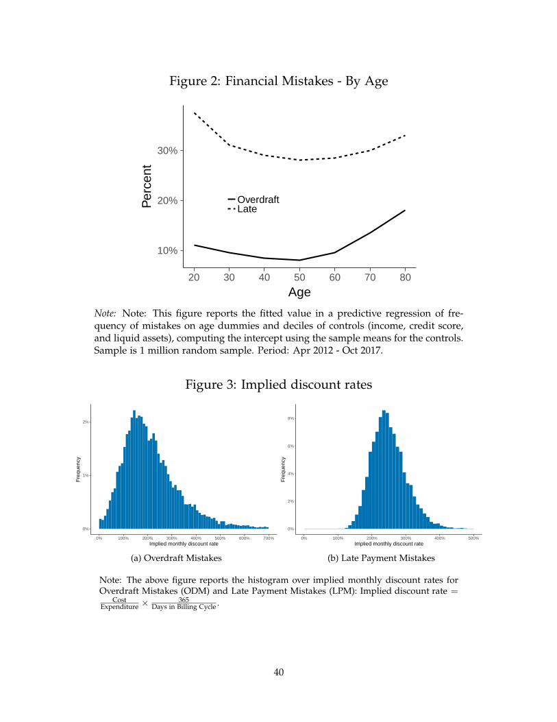
Figure 2: Financial Mistakes - By Age

10%

20%

30%

20 30 40 50 60 70 80

Age

Per

cent

OverdraftLate

Note: Note: This figure reports the fitted value in a predictive regression of fre-quency of mistakes on age dummies and deciles of controls (income, credit score,and liquid assets), computing the intercept using the sample means for the controls.Sample is 1 million random sample. Period: Apr 2012 - Oct 2017.

Figure 3: Implied discount rates

0%

1%

2%

0% 100% 200% 300% 400% 500% 600% 700%Implied monthly discount rate

Fre

quen

cy

(a) Overdraft Mistakes

0%

2%

4%

6%

8%

0% 100% 200% 300% 400% 500%Implied monthly discount rate

Fre

quen

cy

(b) Late Payment Mistakes

Note: The above figure reports the histogram over implied monthly discount rates forOverdraft Mistakes (ODM) and Late Payment Mistakes (LPM): Implied discount rate =

CostExpenditure ×

365Days in Billing Cycle .

40

Figure 4: Mistake cost and frequency

0%

10%

20%

30%

40%

50%

$0 $0−$50 $50−$100 $100−$150 $150−$250 $250+

Average yearly cost ($)

Fre

quen

cy

(a) Late Payment Mistake: Full sample

0%

10%

20%

30%

40%

$0 $0−$50 $50−$100 $100−$150 $150−$250 $250+

Average yearly cost ($)

Fre

quen

cy

(b) Late Payment Mistake: HELOC sample

0%

10%

20%

30%

40%

50%

60%

70%

$0 $0−$50 $50−$100 $100−$150 $150−$250 $250+

Average yearly cost ($)

Fre

quen

cy

(c) Overdraft Mistake: Full sample

0%

10%

20%

30%

40%

50%

60%

70%

$0 $0−$50 $50−$100 $100−$150 $150−$250 $250+

Average yearly cost ($)

Fre

quen

cy

(d) Overdraft Mistake: HELOC sample

0%

10%

20%

30%

$0 $0−$50 $50−$100 $100−$150 $150−$250 $250−$500 $500+

Average yearly cost ($)

Fre

quen

cy

(e) Both mistakes: Full sample

0%

10%

20%

30%

$0 $0−$50 $50−$100 $100−$150 $150−$250 $250−$500 $500+

Average yearly cost ($)

Fre

quen

cy

(f) Both mistakes: Heloc sample

Note: This figure plots the frequency of consumers by average annual cost of the financial mistakes for the periodNovember 2012 to June 2017. Panels (a) and (b) report the frequency sorted by annual cost of the late paymentmistake. Panels (c) and (d) sorted by the annual cost of the overdraft mistake. Panels (e) and (f) sorted on bothmistakes combined. Panels (a), (c), and (e) report frequencies for the full sample, and panels (b), (d), and (f)report for the HELOC sample.

41

Figure 5: Consumption expenditure and HELOC resets– Full Sample

$1,800

$1,850

$1,900

−5 −4 −3 −2 −1 0 1 2 3 4 5 6

Months relative to HELOC reset

Con

sum

ptio

n ex

pend

iture Full sample

Note: This figure plots the fitted value of a regression of total consumptionexpenditure on dummy variables for months relative to HELOC reset, aconstant, person- and calendar-time fixed effects, and decile bins of con-trol variables (income, age, total assets, liquid assets, credit score, andconsumption volatility from t=-5 to t=0).

42

Figure 6: Consumption expenditure and HELOC resets

$1,650

$1,700

$1,750

$1,800

$1,850

$1,900

$1,950

−5 −4 −3 −2 −1 0 1 2 3 4 5 6

Months relative to HELOC reset

Con

sum

ptio

n ex

pend

iture

Zero mistakesQ4 mistakes

Note: This figure plots the fitted value of a regression of total consumptionexpenditure on dummy variables for months relative to HELOC reset, aconstant, person- and calendar-time fixed effects, and decile bins of con-trol variables (income, age, total assets, liquid assets, credit score, andconsumption volatility from t=-5 to t=0).

Figure 7: MPC from predictable positive income change

t

y

c

0

disposable income y

unconstrained consumption c

~c constrained consumption ~c

at+1 = (yt + at − ~ct)(1 + r)

liquidity constraint at ≥ 0

∆~c−∆c > 0

Note: This figure plot the theoretical consumption response to a predictable increase in disposableincome from an unconstrained and a borrowing constrained agent.

43

Figure 8: MPC from predictable negative income change

t

yc = ~c

0

disposable income y

unconstrained consumption c

constrained consumption ~c

c

`ignorant' consumption c

Note: This figure plot the theoretical consumption response to a predictable increase in disposableincome from an unconstrained, a borrowing constrained and rational agent, and from an ignorantagent.

Figure 9: Model calibration

$480

$490

$500

$510

$520

$530

−12 −9 −6 −3 0 3 6 9 12 15 18 21 24Months since debt payment reset

Mon

thly

Exp

endi

ture

on

Nec

essi

ties

LiteracyHigh

Low

Payment Resets and Expenditure on Necessities

(a) Overdraft Mistakes

$480

$490

$500

$510

$520

$530

−12 −9 −6 −3 0 3 6 9 12 15 18 21 24

Months since debt payment reset

Ave

rage

mon

thly

exp

endi

ture

Rational Behavioral Behavioral w. habit

Model Calibration with Identical Income

(b) Late Payment Mistakes

Note: The above figures plot necessity expenditure around HELOC reset date, and thecorresponding calibration of the model. See section 4.1 for a description of the HELOCevent study, and see table A7 for model parameters.

44

Figure 10: Financial Mistakes and Luxury Con-sumption

●

●

●

●

●

● ●

●

●

●

● ●

●

●

●

●

●

●●

●

●

●

●

●

●

●

●

●

●

●

●

● ●

● ●

●

●

●●

●

●

●

●●

●●

●

●

●

●

●●

●

●●

●

●

●●

●

●

●

●●

●

●

25.0%

27.5%

30.0%

32.5%

35.0%

37.5%

$15K $50K $200K $750K

Total Wealth

Luxu

ry a

s pc

t. of

tota

l spe

nd

Note: This figure plot the average spending ratio on luxury goods rel-ative to wealth for two groups of consumers: Consumers who neverincurred avoidable card fees (in blue) and the quartile of consumerswho most frequently have incurred avoidable fees (in red). Luxurygoods are defined as: entertainment, electronics, jewelry and arts, andtravel. The dots represent 30 equal sized bins based on wealth, and thesolid line is a local-linear regression on the entire dataset.

45

Table 1: Characteristics of Customers - entire population

Customers w. Quartiles among positive valueszero mistakes Lowest 2Q 3Q Highest

Age 47 47 45 44 42Annual Income $72,027 $72,607 $69,159 $66,623 $63,298Liquid Assets $24,401 $21,285 $16,337 $12,673 $6,868Total Assets $366,735 $315,267 $261,486 $210,532 $148,465Credit Score 259 215 241 222 2504 Year College 0.38 0.38 0.36 0.34 0.33

Table 2: Characteristics of Customers - HELOC sample

Customers w. Quartiles among positive valueszero mistakes Lowest 2Q 3Q Highest

Age 57 57 58 57 55Annual Income $98,164 $99,207 $98,760 $99,270 $97,285Liquid Assets $33,408 $31,210 $28,507 $23,950 $14,603Total Assets $705,571 $647,178 $583,216 $495,489 $348,471Credit Score 339 255 306 302 3374 Year College 0.40 0.40 0.39 0.39 0.37

Note: The above two tables report mean values sorted by frequency of Late-payment-mistakes (LPM) and Overdraft-payment-mistakes (ODM) over the pe-riod 2012-2017. The first table is The first column represents the 31% of consumerswho in the period have neither an LPM nor an ODM. The next four columns aresorted in quartiles by frequency of LPM and ODM.

46

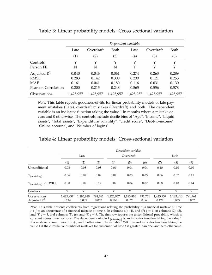
Table 3: Linear probability models: Cross-sectional variation

Dependent variable:

Late Overdraft Both Late Overdraft Both

(1) (2) (3) (4) (5) (6)

Controls Y Y Y Y Y YPerson FE N N N Y Y Y

Adjusted R2 0.040 0.046 0.061 0.274 0.263 0.289RMSE 0.283 0.142 0.300 0.239 0.121 0.253MAE 0.161 0.041 0.180 0.116 0.031 0.130Pearson Correlation 0.200 0.215 0.248 0.565 0.556 0.578

Observations 1,425,957 1,425,957 1,425,957 1,425,957 1,425,957 1,425,957

Note: This table reports goodness-of-fits for linear probability models of late pay-ment mistakes (Late), overdraft mistakes (Overdraft) and both. The dependentvariable is an indicator function taking the value 1 in months where a mistake oc-curs and 0 otherwise. The controls include decile bins of "Age", "Income", "Liquidassets", "Total assets", "Expenditure volatility", "credit score", "Debt-to-income","Online account", and "Number of logins".

Table 4: Linear probability models: Cross-sectional variation

Dependent variable:

Late Overdraft Both

(1) (2) (3) (4) (5) (6) (7) (8) (9)

Unconditional 0.08 0.08 0.08 0.04 0.04 0.04 0.10 0.10 0.10

1{mistakeit} 0.06 0.07 0.09 0.02 0.03 0.05 0.06 0.07 0.11

1{mistakeit} × TWICE 0.08 0.09 0.12 0.02 0.04 0.07 0.08 0.10 0.14

Controls Y Y Y Y Y Y Y Y Y

Observations 1,425,957 1,183,810 791,761 1,425,957 1,183,810 791,761 1,425,957 1,183,810 791,761Adjusted R2 0.124 0.085 0.057 0.160 0.073 0.060 0.172 0.063 0.052

Note: This table presents coefficients from regressions relating the probability of a financial mistake at timet + j to an occurrence of a financial mistake at time t. In columns (1), (4), and (7) j = 1, in columns (2), (5),and (8) j = 3, and columns (3), (6), and (9) j = 9. The first row reports the unconditional probability which isconstant across time horizons. The dependent variable 1{mistakeit} is an indicator function taking the value 1if a mistake occurs in month t + j and 0 otherwise. The variable TWICE is and indicator function taking thevalue 1 if the cumulative number of mistakes for customer i at time t is greater than one, and zero otherwise.

47

Table 5: Correlation across multiple mistakes: Avoidable LateFees

Customers w. Quartiles among positive valueszero mistakes Lowest 2Q 3Q Highest

Avoidable overdraft fees 36% 51% 55% 61% 68%CC spending mistake 74% 77% 76% 79% 82%CC payment mistake 54% 60% 59% 62% 66%Mortgage non-optimal 87% 91% 91% 90% 93%Investment non-participation 92% 97% 97% 98% 98%

Table 6: Correlation across multiple mistakes: Avoidable Over-draft Fees

Customers w. Quartiles among positive valueszero mistakes Lowest 2Q 3Q Highest

Avoidable late fees 55% 59% 60% 59% 62%CC spending mistake 73% 76% 77% 80% 81%CC payment mistake 54% 60% 59% 61% 65%Mortgage non-optimal 88% 91% 91% 91% 92%Investment non-participation 93% 96% 97% 97% 98%

Note: The above two tables report frequency of various financial mistakes sorted on fre-quency of avoidable late and overdraft fees. For avoidable late fees is reports the frequencyof avoidable overdraft fees, credit card spending mistakes, credit card payment mistakes,lack of mortgage refinancing, and non-participation in investment accounts. For avoidableoverdraft fees it reports avoidable late fees, credit card spending mistakes, credit card pay-ment mistakes, lack of mortgage refinancing, and non-participation in investment accounts.

48

Table 7: Characteristics of Customers - Demographics andIncome

Customers w. zero mistakes Q4 by mistakes frequency(31% of sample) (17% of sample)

Demographics and IncomeAge 58 55Income $98,164 $97,285∆ Income in past 6 months $792 $719Unemployment in past 6 months 2% 2%Financial ChoicesCredit Score 339 337Total Assets $705,871 $348,471Liquid Assets $32,008 $9,624Investment Account 19% 5%

Note: This tables report the mean values for the HELOC sample of Age, Income,Change in income over past six months, unemployment rate over past six months,internal credit score, total assets, liquid assets, and percentage of consumers whohave an investment account. The two groups of consumers compared are sortedby frequency of the two benchmark financial mistakes on the last month of theirHELOC draw period.

49

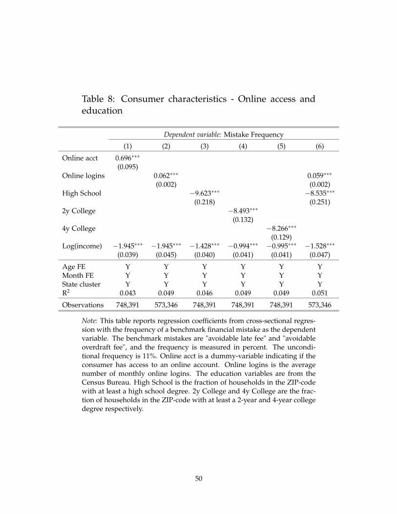
Table 8: Consumer characteristics - Online access andeducation

Dependent variable: Mistake Frequency

(1) (2) (3) (4) (5) (6)

Online acct 0.696∗∗∗

(0.095)Online logins 0.062∗∗∗ 0.059∗∗∗

(0.002) (0.002)High School −9.623∗∗∗ −8.535∗∗∗

(0.218) (0.251)2y College −8.493∗∗∗

(0.132)4y College −8.266∗∗∗

(0.129)Log(income) −1.945∗∗∗ −1.945∗∗∗ −1.428∗∗∗ −0.994∗∗∗ −0.995∗∗∗ −1.528∗∗∗

(0.039) (0.045) (0.040) (0.041) (0.041) (0.047)

Age FE Y Y Y Y Y YMonth FE Y Y Y Y Y YState cluster Y Y Y Y Y YR2 0.043 0.049 0.046 0.049 0.049 0.051

Observations 748,391 573,346 748,391 748,391 748,391 573,346

Note: This table reports regression coefficients from cross-sectional regres-sion with the frequency of a benchmark financial mistake as the dependentvariable. The benchmark mistakes are "avoidable late fee" and "avoidableoverdraft fee", and the frequency is measured in percent. The uncondi-tional frequency is 11%. Online acct is a dummy-variable indicating if theconsumer has access to an online account. Online logins is the averagenumber of monthly online logins. The education variables are from theCensus Bureau. High School is the fraction of households in the ZIP-codewith at least a high school degree. 2y College and 4y College are the frac-tion of households in the ZIP-code with at least a 2-year and 4-year collegedegree respectively.

50

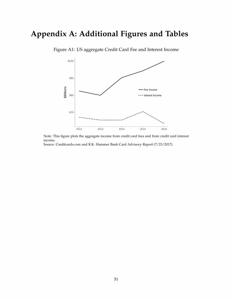
Appendix A: Additional Figures and Tables

Figure A1: US aggregate Credit Card Fee and Interest Income

$70

$80

$90

$100

2012 2013 2014 2015 2016

$Bill

ions Fee Income

Interest Income

Note: This figure plots the aggregate income from credit card fees and from credit card interestincome.Source: Creditcards.com and R.K. Hammer Bank Card Advisory Report (7/23/2017).

51

Figure A2: IO HELOC example

This figure plots an example of a payment schedule from an Interest Only Home Equity Line ofCredit. Source: Creditcards.com (7/23/2017).

Figure A3: HELOC - Placebo tests

−50

0

−12 −9 −6 −3 0 3 6 9 12 15 18 21 24

Months relative to 'HELOC reset'

Diff

eren

ce b

etw

een

grou

ps

heloc

placebo1

placebo2

placebo3

Note: This figure represents three placebo tests for the impact of HELOC reset on credit cardexpenditure. The solid line represents the difference in credit card expenditure in the aroundthe true HELOC reset dates. Placebo1 has start-year=3, Placebo2 has start-year=6, and Placebo3has start-year=15.

52

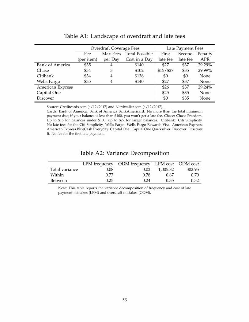
Table A1: Landscape of overdraft and late fees

Overdraft Coverage Fees Late Payment FeesFee Max Fees Total Possible First Second Penalty

(per item) per Day Cost in a Day late fee late fee APRBank of America $35 4 $140 $27 $37 29.29%Chase $34 3 $102 $15/$27 $35 29.99%Citibank $34 4 $136 $0 $0 NoneWells Fargo $35 4 $140 $27 $37 NoneAmerican Express $26 $37 29.24%Capital One $25 $35 NoneDiscover $0 $35 None

Source: Creditcards.com (4/12/2017) and Nerdwallet.com (4/12/2017).Cards: Bank of America: Bank of America BankAmericard. No more than the total minimumpayment due; if your balance is less than $100, you won’t get a late fee. Chase: Chase Freedom.Up to $15 for balances under $100; up to $27 for larger balances. Citibank: Citi Simplicity.No late fees for the Citi Simplicity. Wells Fargo: Wells Fargo Rewards Visa. American Express:American Express BlueCash Everyday. Capital One: Capital One Quicksilver. Discover: DiscoverIt. No fee for the first late payment.

Table A2: Variance Decomposition

LPM frequency ODM frequency LPM cost ODM costTotal variance 0.08 0.02 1,005.82 302.95Within 0.77 0.78 0.67 0.70Between 0.25 0.24 0.35 0.32

Note: This table reports the variance decomposition of frequency and cost of latepayment mistakes (LPM) and overdraft mistakes (ODM).

53

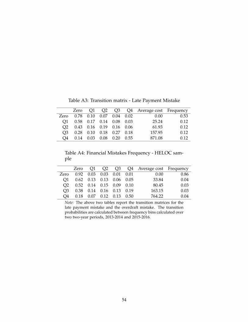
Table A3: Transition matrix - Late Payment Mistake

Zero Q1 Q2 Q3 Q4 Average cost FrequencyZero 0.78 0.10 0.07 0.04 0.02 0.00 0.53

Q1 0.58 0.17 0.14 0.08 0.03 25.24 0.12Q2 0.43 0.16 0.19 0.16 0.06 61.93 0.12Q3 0.28 0.10 0.18 0.27 0.18 157.95 0.12Q4 0.14 0.03 0.08 0.20 0.55 871.08 0.12

Table A4: Financial Mistakes Frequency - HELOC sam-ple

Zero Q1 Q2 Q3 Q4 Average cost FrequencyZero 0.92 0.03 0.03 0.01 0.01 0.00 0.86

Q1 0.62 0.13 0.13 0.06 0.05 33.84 0.04Q2 0.52 0.14 0.15 0.09 0.10 80.45 0.03Q3 0.38 0.14 0.16 0.13 0.19 163.15 0.03Q4 0.18 0.07 0.12 0.13 0.50 764.22 0.04Note: The above two tables report the transition matrices for thelate payment mistake and the overdraft mistake. The transitionprobabilities are calculated between frequency bins calculated overtwo two-year periods, 2013-2014 and 2015-2016.

54

Table A5: Financial Mistakes Frequency - entire population

Month Customers Share of fees Share of feesw. zero w. zero avoidable (ew) avoidable (vw)

Avoidable late fee 0.92 0.42 0.94 0.92Avdbl. overdraft 0.96 0.66 0.81 0.75CC payment 0.64 0.40 0.46 0.01CC spending 0.62 0.23 0.48 0.04

Table A6: Financial Mistakes Frequency - HELOC sample

Month Customers Share of fees Share of feesw. zero w. zero avoidable (ew) avoidable (vw)

Avoidable late fee 0.93 0.43 0.96 0.95Avdbl. overdraft 0.97 0.72 0.78 0.73CC payment 0.67 0.42 0.44 0.01CC spending 0.62 0.23 0.52 0.04

Note: The above two tables report the frequency of four financial mistakesacross the entire population and the HELOC sub sample respectively. Thefirst column reports the fraction of months where no mistake is observed,and the second column reports the fraction of customers who never incurthe respective mistake from 2012-2016. The third column is calculated asthe fraction of months with avoidable mistakes relative to the number ofmonths with a finance charge in the same category. The last column iscalculated similarly to the third, but weighted by the dollar amount of thefinance charge.

Table A7: Model calibration

Parameter Definition Value Target/Sourceβ Discount factor 0.9

112 See text

σ Coefficient of relative risk aversion 12 Hall (2011)

ε Intertemporal elasticity of substitution 1 Schmidt et al. (2017)φ Relative taste for luxuries 0.3 Mean luxury expenditure fractionρ Persistence of income shock 0.95 See text.σ2 Variance of income shock 0.05 See text.π f Job finding rate 0.08 Shimer (2005)πs Job seperation rate 0.01 Shimer (2005)ν Unemployment benefit 0.4 40% of average labor income.

Note: All variables are calibrated monthly.

55

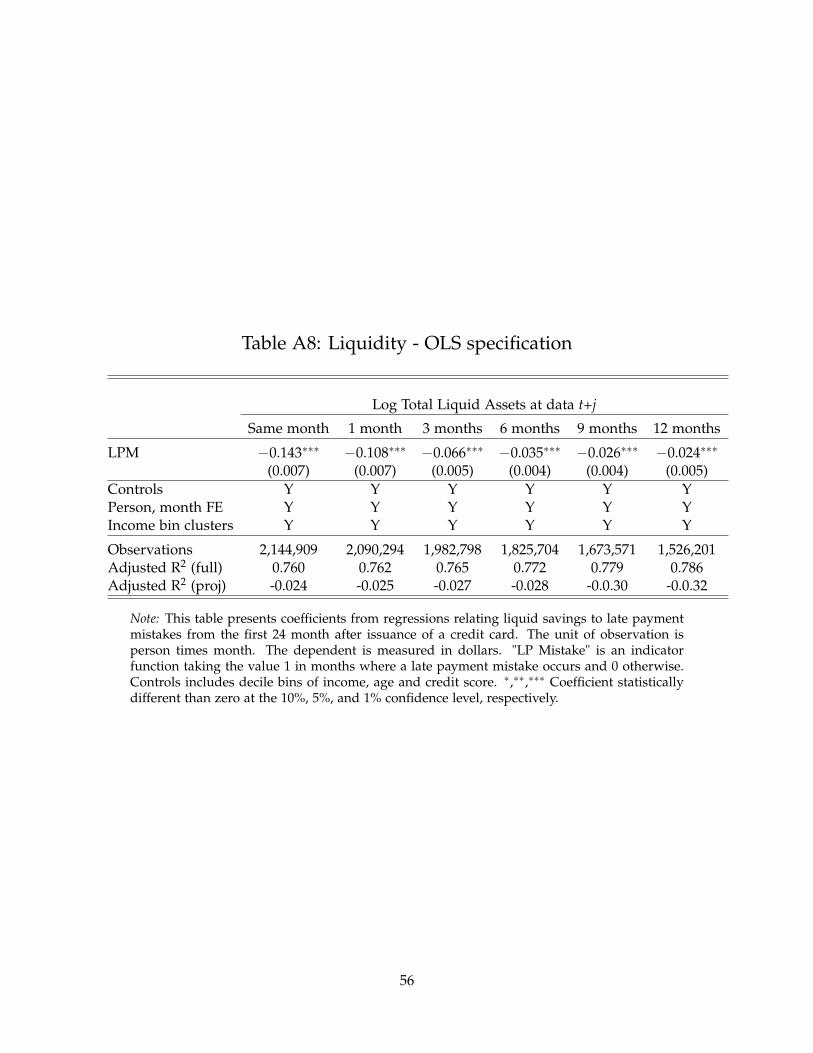
Table A8: Liquidity - OLS specification

Log Total Liquid Assets at data t+j

Same month 1 month 3 months 6 months 9 months 12 months

LPM −0.143∗∗∗ −0.108∗∗∗ −0.066∗∗∗ −0.035∗∗∗ −0.026∗∗∗ −0.024∗∗∗

(0.007) (0.007) (0.005) (0.004) (0.004) (0.005)Controls Y Y Y Y Y YPerson, month FE Y Y Y Y Y YIncome bin clusters Y Y Y Y Y Y

Observations 2,144,909 2,090,294 1,982,798 1,825,704 1,673,571 1,526,201Adjusted R2 (full) 0.760 0.762 0.765 0.772 0.779 0.786Adjusted R2 (proj) -0.024 -0.025 -0.027 -0.028 -0.0.30 -0.0.32

Note: This table presents coefficients from regressions relating liquid savings to late paymentmistakes from the first 24 month after issuance of a credit card. The unit of observation isperson times month. The dependent is measured in dollars. "LP Mistake" is an indicatorfunction taking the value 1 in months where a late payment mistake occurs and 0 otherwise.Controls includes decile bins of income, age and credit score. ∗,∗∗,∗∗∗ Coefficient statisticallydifferent than zero at the 10%, 5%, and 1% confidence level, respectively.

56

Table A9: Liquidity - DID specification

Log Total Liquid Assets at data t+j

Same month 1 month 3 months 6 months 9 months 12 months

LPM −0.091∗∗∗ −0.067∗∗∗ −0.029∗∗∗ −0.026∗∗∗ −0.017∗ −0.023∗∗

(0.011) (0.009) (0.011) (0.009) (0.010) (0.009)POST −0.029∗∗∗ −0.025∗∗∗ −0.013∗∗ −0.001 −0.008 −0.010

(0.007) (0.006) (0.005) (0.007) (0.010) (0.012)LPM × POST −0.076∗∗∗ −0.050∗∗∗ −0.038∗∗∗ −0.002 −0.010 −0.012

(0.012) (0.013) (0.012) (0.013) (0.008) (0.012)Person, month FE Y Y Y Y Y YIncome bin clusters Y Y Y Y Y Y

Observations 2,144,909 2,090,294 1,982,798 1,825,704 1,673,571 1,526,201Adjusted R2 (full) 0.772 0.772 0.775 0.781 0.786 0.793Adjusted R2 (proj) -0.024 -0.025 -0.027 -0.028 -0.0.30 -0.0.32

Note: This table presents coefficients from regressions relating liquid savings to latepayment mistakes from the first 24 month after issuance of a credit card. The unitof observation is person-month. The dependent varialbe is measured in dollars. "LPMistake" is an indicator function taking the value 1 in months where a late paymentmistake occurs and 0 otherwise. POST is an indicator variable taking the value 1 inmonths 13-24 and 0 otherwise. $LPM is the measured cost of a late payment mistake.∗,∗∗,∗∗∗ Coefficient statistically different than zero at the 10%, 5%, and 1% confidencelevel, respectively.

Table A10: Liquidity - OLS in levels

Log Total Liquid Assets at data t+j

Same month 1 month 3 months 6 months 9 months 12 months

$LPM −0.002∗∗∗ −0.002∗∗∗ −0.001∗∗∗ −0.001∗∗∗ −0.0005∗∗∗ −0.0004∗∗∗

(0.0002) (0.0002) (0.0001) (0.0001) (0.0001) (0.0001)Person, month FE Y Y Y Y Y YIncome bin clusters Y Y Y Y Y Y

Observations 2,144,909 2,090,294 1,982,798 1,825,704 1,673,571 1,526,201Adjusted R2 (full) 0.760 0.762 0.765 0.772 0.779 0.786Adjusted R2 (proj) -0.024 -0.025 -0.027 -0.028 -0.0.30 -0.0.32

Note: ∗p<0.1; ∗∗p<0.05; ∗∗∗p<0.01

57

Table A11: Liquidity - IV in levels

Log Total Liquid Assets at data t+j

Same month 1 month 3 months 6 months 9 months 12 months

$LPM −0.002∗∗∗ −0.001∗∗∗ −0.001∗∗∗ −0.0004∗∗∗ −0.0003∗∗ −0.0002∗∗

(0.0002) (0.0002) (0.0002) (0.0001) (0.0001) (0.0001)Person, month FE Y Y Y Y Y YIncome bin clusters Y Y Y Y Y Y

Observations 791,761 772,884 735,222 679,730 626,343 575,001Adjusted R2 (full) 0.772 0.772 0.775 0.781 0.786 0.793Adjusted R2 (proj) -0.024 -0.025 -0.027 -0.028 -0.0.30 -0.0.32

Note: ∗p<0.1; ∗∗p<0.05; ∗∗∗p<0.01

58

Appendix B: Test of causal effect on liquidityIn order to analyze the effect of an avoidable fee on liquidity I use a difference-in-

difference research design. The DID design uses relies on the contractual discontinuity whichmeans that the penalty APR is only levied after the first 12 months.

In this section I estimate the causual impact of paying an avoidable fee on a consumer’sliquid assets. I use a difference-in-difference research design that explores an institutionalfeature of the cost of late payments: Recall that the Late Payment Mistake (LPM) occurs whena consumer fails to pay the minimum payment AND the consumer has sufficient deposits(over and above precautionary savings). When a consumer fails to pay the minimum balance,he is officially in violation of the contract, and two things occur: (1) He receives a late fee, and(2) the interest rate on the outstanding balance increases to the penalty apr. In appendix tableA1 we see examples of penalty APRs. Penalty APRs are legally capped at 29.99% as per theCARD acct.

As an illustrative example consider a consumer who has an outstanding balance of $1,000,with a minimum payment due of $25. Regular APR=18%, Penalty APR=29.99%, and LateFee=$35. He considers the following two options:

a) Only pay the minimum balance of $25, and thus borrow $975 for one month.

b) Not pay anything: borrow $1,000 for one month.

The cost of these two options after one month are as follows:

a) Total Finance Charge = 18%/12*$975 = $14.63

b) Total Finance Charge = 29.99%/12*$1,035 + $35 = $60.87

We see that the consumer will pay an additional $46 just to avoid paying the minimumpayment of $25. That is equal to an implied a one-month interest rate of 185% (which is inline with the histogram of implied discount rates, see figure 3) .

Given this example, we want to ask: what is the causal impact of making a late paymentmistake on end-of-month liquid assets. There is an obvious endogeneity concern: A customermakes the late payment mistake when he is not paying his credit card statement, which mightcorrelate endogeneously with a negative liquidity shock. The solution is to use exogenousvariation in the cost of the late payment mistake from the Penalty APR. The CARD act hasenforced that in the first 12 months after opening a card, no Penalty APR can be imposed.This offers a natural difference-in-difference research design where I can compare mistakesmade in the first 12 months with mistakes made in months 13-24. Of course the identifyingassumption is that customers are similar on unobservables that would affect liquidity inmonths 1-12 vs. months 13-24.

59

Table A12: Liquid Savings and Late Payment Mistakes

Dependent variable:

End-of-month liquid savings Liquid savings after 3 months

(1) (2) (3) (4) (5) (6)

LP Mistake −0.143∗∗∗ −0.091∗∗∗ −0.029∗∗∗

(0.007) (0.011) (0.011)POST −0.029∗∗∗ −0.013∗∗∗

(0.007) (0.005)LP Mistake × POST −0.076∗∗∗ −0.038∗∗∗

(0.012) (0.012)$LPM −0.002∗∗∗ −0.002∗∗∗ −0.001∗∗∗

(0.0001) (0.0002) (0.0002)Specification OLS DID OLS IV DID IVPerson, month FE Y Y Y Y Y YIncome bin clusters Y Y Y Y Y Y

Observations 2,144,909 791,761 791,761 791,761 791,761 791,761Adjusted R2 (full) 0.760 0.772 0.760 0.772 0.772 0.772Adjusted R2 (proj) -0.024 -0.025 -0.027 -0.028 -0.027 -0.030

Note: This table presents coefficients from regressions relating liquid savings to late pay-ment mistakes from the first 24 month after issuance of a credit card. The unit of observa-tion is person-month. The dependent varialbe is measured in dollars. "LP Mistake" is anindicator function taking the value 1 in months where a late payment mistake occurs and0 otherwise. POST is an indicator variable taking the value 1 in months 13-24 and 0 other-wise. $LPM is the measured cost of a late payment mistake. ∗,∗∗,∗∗∗ Coefficient statisticallydifferent than zero at the 10%, 5%, and 1% confidence level, respectively.

60

Table (A12) reports the results. Following the methodology of Agarwal et al. (2015a) andAgarwal et al. (2016) I report the regression coefficients for each of the regression specifica-tions across the entire time horizon. These can be found in appendix tables A9, A10, andA11.

61

Appendix C: Numerical Method

Financially ignorant households - decision problem

Here I outline the procedure to calculate the optimal attention paid to future financialvariables following Tibshirani 1996 and Gabaix 2014, 2016:

First, let mt ∈ [0, 1] denote attention weight to payment difference x. Now, two solve thehouseholds decision problem I must solve a two-step problem:

1. Choose weight mt

2. Solve C-S problem with xst ≡ mtxt

In order to solve this problem we first define out standard value function (capital V):

Vt(zt) = maxct

{u(ct, zt) + βE[V(zt+1)]

}with state variables: zt = {at, yt, bt, xt}, a choice variable: ct, and a transition function: zt+1 =

F(ct, zt, εt+1)

Next define lower case ’v’:

v(ct, zt) = u(ct, zt) + βE[V(zt+1)], (.1)

and consider a 2nd order Taylor approximation around m = 0.Now, let the default attention and consumption be md = 0 and cd = arg maxc v(x, z, md),

and let cm ≡ ∂c∂m |(md,cd). The sparse max operator, smaxc,m is defined by the following proce-

dure (Gabaix, 2014, 2016a,b):Step 1: Choose the attention vector m∗:

m∗ = arg minm∈[0.1]

12

Λ(1−m)2 + κm (.2)

with the cost-of-inattention factor Λ ≡ −E[cmVcccm]

Step 2: Choose choice variables

cs = arg maxc

v(c, z, m∗) (.3)

and have the resulting utility be vs = v(cs, z).

In the numerical exercise, for every simulation draw I follow the following procedure(outlined in Ganong and Noel (2016)) to solve for the optimal attention to the HELOC resetgiven a κ:

62

1. Compute ct(zt) as the consumption level, so z equals actual income at t = 0.

2. Compute dcdm as the change in consumption from additional attention.

3. For grid values of κ:

(a) For a seed value of z, compute ct(z).

(b) Compute optimal attention m∗ using equation 5.7.

(c) Calculate perceived income at HELOC reset date T.

(d) At each date t ≤ T the consumer forms a consumption plan c∗t using perceived zt.

(e) If the quadratic distance between c∗t (m∗t ) and ct is less than 0.0001 continue to the

next value in the grid of κ.

(f) If not, return to step (a) with an alternate value of z.

4. Evaluate distance from generated {c∗t (m∗)} to the data. Choose m∗ that best fits data.

63