The Cost of Capital for Alternative Investments

Jakub W. Jurek and Erik Stafford∗

Abstract

We develop a simple state-contingent framework for evaluating the cost of capital for non-linear

risk exposures, and show that properly computed required rates of return are meaningfully higher than

indicated by linear factor models. Given the large allocations of typical investors in alternatives, many

have not covered their cost of capital, despite earning an annualized excess return of 6.3% between

1996 and 2010. A simple derivative-based strategy, which accurately matches the risk profile of hedge

funds, realizes an annualized excess return of 9.7% over this sample period, while providing monthly

liquidity and complete transparency over its state-contingent payoffs. Linear clones based on popular

factor models deliver annualized risk premia of 0-3% over the same period.

First draft: June 2011

This draft: April 2012

∗Jurek: Bendheim Center for Finance, Princeton University; jjurek@princeton.edu. Stafford: Harvard Business School;estafford@hbs.edu. We thank Joshua Coval, Ken French, Samuel Hanson, Jonathan Lewellen, Burton Malkiel, Robert Merton,Gideon Ozik (discussant), Andre Perold, Jeremy Stein, Marti Subrahmanyam (discussant), and seminar participants at Dart-mouth College, Harvard Business School, Imperial College, Bocconi University, USI Lugano, Princeton University, the 2011NYU Five-Star Conference, and the 4th NYSE Liffe Hedge Fund Research Conference for helpful comments and discussions.

This paper studies the required rate of return for a risk averse investor allocating capital to alternative

investments. There are two key aspects to this asset allocation decision that present a challenge for standard

decision-making tools. First, the alternative investment exposure is nonlinear with respect to the remainder

of the portfolio at the horizon where the investor is able to rebalance the portfolio, making static mean-

variance analysis inappropriate. Second, the typical allocation is large relative to the aggregate outstanding

share in the economy, such that charging for a marginal deviation from an equilibrium allocation is a poor

approximation of the actual contribution to the portfolio’s overall risk. These two features interact to

produce very large required rates of return relative to commonly used factor models, including recent

models designed to deal with the payoff nonlinearity.

One important aspect of the real world problem of assessing the performance of alternative investments

is that – conditional on investing in alternatives – typical allocations are large relative to the equilibrium

supply of the risks. For example, as of June 2010, the Ivy League endowments had 40% of their combined

assets allocated to non-traditional assets (Lerner, et al. (2008)), whereas the share of alternatives in the

global wealth portfolio was closer to 2%.1 The traditional approach to performance evaluation uses linear

factor regressions (e.g. CAPM, Fama-French 3-factor model, Fung-Hsieh 9-factor model, and conditional

variations thereof) to decompose realized asset excess returns into alpha and compensation for bearing

risk. The product of the estimated loadings, or betas, and the factor risk premia, represents the model

estimate of the required rate of return. This estimate is interpretable as the excess rate of return that

would be required by an investor making a marginal deviation from his existing equilibrium allocation.

Therefore, the findings from linear factor analyses – that hedge funds exhibit positive and statistically

significant alphas (Agarwal and Naik (2004), Fung and Hsieh (2004), Hasanhodzic and Lo (2007)) – say

little about whether the investor with a 40% allocation is getting a good or bad deal.2

The primary goal of this paper is to explore the interaction of large allocations and payoff non-linearities

on the investor’s cost of capital, in order to better match the nature of the real world problem. To derive

estimates of the cost of capital in this setting, we assemble a simple static portfolio selection framework

that combines power utility (CRRA) preferences, with a state-contingent asset payoff representation, in

the spirit of Arrow (1964) and Debreu (1959). We specify the joint structure of asset payoffs by describing

1As of end of 2010, the total assets under management held by hedge funds stood at roughly $2 trillion (source: HFRI),in comparison to a combined global equity market capitalization of $57 trillion (source: World Federation of Exchanges) anda combined global bond market capitalization of $54 trillion, excluding the value of government bonds (source: TheCityUK,“Bond Markets 2011”).

2The factor regressions are only correctly specified if the relationship between the equilibrium stochastic discount factorand the set of risk factors, which characterize changes in marginal utility, is linear. In many static models, marginal utilityis not linear in the factors, and a linear relationship can only be obtained as a Taylor approximation, or by assuming normaldistributions; linear factor models also arise naturally in the limit of continuous time (Cochrane (2005)). Given investors inalternatives cannot adjust their exposures frequently, and the well-established evidence of non-linearity in hedge fund returns,neither of the last two scenarios applies.

1

each security’s payoff as a function of the aggregate equity index (here, the S&P 500).3 To capture the

non-linear risk exposure of alternatives, we model hedge fund returns as a portfolio of cash and a short

position in a single equity index put option.4 The contractual nature of index put options immediately

provides a complete state-contingent description of an investable alternative to the aggregate hedge fund

universe. In turn, the availability of a state-contingent risk profile allows us to determine the rate of return

that an investor would require as a function of his risk aversion, portfolio allocation, and the underlying

return distributions of other asset classes, all of which are necessary for any asset allocation decision. An

additional reason for focusing on index put writing strategies is that these are likely to earn large economic

risk premia due to their systematic crash and liquidity risk exposures, which are concentrated in economic

states associated with high marginal utility.5 To the extent that hedge fund strategies are capturing these

types of non-traditional risk premia, replication strategies that simply form linear mixtures of assets that

are not exposed to these risks will not earn these premia.

Our empirical strategy for describing the risks of the aggregate hedge fund index focuses on index

derivatives since they are the traded securities that are most highly exposed to the non-traditional crash

and systematic liquidity risks. The challenge is specifying the proper exposure to these non-traditional

factors. We do not have a structural relation to estimate. Instead, we calibrate the theoretical exposure

of various derivative strategies by first matching the known traditional risks of the hedge fund index as

measured by linear factor models. Specifically, we focus our attention on strategies that have an ex ante

theoretical CAPM beta at inception equal to the estimated CAPM beta of the HFRI Fund-Weighted

Composite (β ≈ 0.4). We then evaluate whether these simple portfolios of cash and index derivatives,

or non-linear clones, accurately capture the risk properties of the aggregate hedge fund universe over the

period from January 1996 to December 2010.

We find that all four of the considered put-writing strategies match well the realized time series risk

properties of the aggregate hedge fund universe in terms of drawdown patterns, including the severe

drawdown realized at the end of 2008, when the S&P 500 index dropped over 50%. Over this period,

the hedge fund index lost 21% of its value, while the drawdowns from the various put-writing strategies

ranged from -22.4% to -20.7%. One of the put writing strategies is preferred in terms of matching realized

3The same state-contingent payoff model is used in Coval, et al. (2009) to value tranches of collateralized debt obligationsrelative to equity index options, and in Jurek and Stafford (2011) to elucidate the time series and cross-section of repo marketspreads and haircuts.

4Empirical evidence that hedge fund returns exhibit nonlinear systematic risk exposures resembling those of index putwriting is provided by Mitchell and Pulvino (2001) for risk arbitrage, and Agarwal and Naik (2004) for a large number ofequity-oriented strategies. Fung and Hsieh (1997, 2001) introduce factors that are long straddles to capture the returns totrend following strategies.

5Option returns reflect the returns to bearing jump and volatility risk (e.g. Carr and Wu (2009), Todorov (2010)), as wellas, compensation for systematic demand imbalances (e.g. Garleanu, et al. (2009), Constantinides, et al. (2012)). He andKrishnamurthy (2012) highlight the role of time-varying capital constraints of intermediaries on asset prices.

2

volatility and CAPM beta over the sample. We find that the preferred strategy matches the overall risk

properties of the hedge fund index at least as well as popular linear factor models. However, the average

annualized excess returns to the preferred nonlinear hedge fund clone are large (9.7% per year) relative

to those of the linear clones, which have average annualized risk premia ranging from 0% to 3% per year.

This large difference meaningfully alters inferences about the abnormal returns (alpha) to hedge funds,

which realize average annualized excess returns of 6.5% over this sample period.

The highly parsimonious and seemingly accurate description of hedge fund risks as index derivatives

allows us to study required rates of returns for these investments for a variety of investors who differ in

their risk aversion and portfolio compositions. The comparative statics of the generalized asset allocation

framework suggest that the nonlinearity of alternative investments creates several differences relative to

the mean-variance framework, and importantly, that these differences become economically meaningful

as the allocation to alternatives increases. For example, our model indicates that over the span of our

sample (1996-2006), the mean ex ante cost of capital for investors who held 35% of their risky portfolio

share in alternatives ranges from 4.9% (equity investor, γ = 2) to 6.9% (endowment investor, γ = 3.3). In

contrast, an investor reliant on a linear CAPM rule would have computed a mean ex ante cost of capital

of only 2.9% per year. Given their large allocations, we show that many investors in hedge funds have not

covered their cost of capital, even if they managed to earn the returns of the survivorship-biased index.

Finally, an interesting implication that emerges from our analysis is that investors relying on traditional

analyses for benchmarking alternatives (e.g. linear factor regression) are likely to be attracted ex ante to

strategies and historical return series that correspond to highly levered investments in safe assets that will

be disappointing in the event of a market crash. Despite appearing to have low linear market exposures,

these strategies command high required rates of return, because they reallocate losses to states in which

marginal utility is high.

The remainder of the paper is organized as follows. Section 1 describes the risk profile of hedge funds.

Section 2 presents a simple recipe for replicating the aggregate hedge fund risk exposure with index put

options and empirically compares the returns of this replication strategy with those produces by linear

factor models. Section 3 develops a generalized asset allocation rule appropriate for combining securities

with nonlinear payoff functions. Section 4 discusses implications of the framework relative to traditional

linear factor models and mean-variance analysis. Finally, Section 5 concludes the paper.

3

1 Describing the Risk Profile of Hedge Funds

To compute the required rate of return – or cost of capital – for an allocation to hedge funds, one must

first characterize the risk profile of a typical investment. Rather than examine risk exposures of individual

funds (Lo and Hasanhodzic (2007)) or strategies (Fung and Hsieh (2001), Mitchell and Pulvino (2001),

Agarwal and Naik (2004), we focus on the aggregate risk properties of the asset class. Consequently, the

cost of capital we derive can be thought of as applying to an investor in a diversified hedge fund portfolio

(e.g. a fund-of-funds, or an endowment holding a portfolio of alternative investments).

We proxy the performance of the hedge fund universe using two indices: the Dow Jones Credit Suisse

Broad Hedge Fund Index, and the HFRI Fund Weighted Composite Index. Such indices are not investable,

and typically provide an upward biased assessment of hedge fund performance due to the presence of backfill

and survivorship bias. For example, Malkiel (2005) reports that the difference between the mean annual

fund return in the backfilled and non-backfilled TASS database was 7.34% per year in the 1994-2003

sample. Moreover, once defunct funds are added in the computation of the mean annual returns to correct

for survivorship bias, the mean annual fund return declines by 4.42% (1996-2003). Consistent with this

evidence, the returns of funds-of-funds – which represent a feasible alternative investment strategy – trail

those of the broad hedge fund indices by roughly 3% per year. To the extent that the survivorship bias

also affects the measured risks, it is unlikely that the true risks are lower than those estimated from the

realized returns over this period. We discuss the implications of higher underlying risks and how alternative

economic outcomes are likely to affect the risks of alternative investments in Section 4.

Table 1 reports summary statistics for the two indices computed using quarterly returns from 1996:Q1-

2010:Q4 (N = 60 quarters), and compares them to the S&P 500 index.6 The attraction of hedge funds over

this time period is clear: mean returns on alternatives exceeded that of the S&P 500 index, while incurring

lower volatility. Moreover, the estimated linear systematic risk exposures (or CAPM β values) indicate that

hedge fund performance was largely unrelated to the performance of the public equity index, and suggests

that relative to this risk model they have outperformed. The realized Sharpe ratios on alternatives were

two and a half times higher than that of the S&P 500 index. Under all of the standard risk metrics inspired

by the mean-variance portfolio selection criterion, hedge funds represented a highly attractive investment.

This is further illustrated in Figure 1, which plots the value of $1 invested in the various assets through

time. By December 2010, the hedge fund investor had amassed a wealth roughly 50% larger than the

wealth of the investor in public equity markets, and more than twice the wealth of an investor rolling over

investments in short-term T-bills.

6Although the indices are available at daily and monthly frequencies, we focus on quarterly returns to ameliorate the effectsof stale prices and return smoothing (Asness, et al. (2001), Getmansky, et al. (2004)).

4

Another risk metric popular among practitioners is the drawdown, which measures the magnitude of

the strategy loss relative to its highest historical value (or high watermark). Hedge funds perform relatively

well on this measure over the sample period with a drawdown of approximately -20%, which is less than

half of the -50% drawdown sustained by investors in public equity markets.

Figure 1 also demonstrates that the performance of hedge funds as an asset class is not market-neutral.

For example, hedge funds experience severe declines during extreme market events, such as the credit crisis

during the fall of 2008 and the LTCM crisis in August 1998. During the two-year decline following the

bursting of the Internet bubble, hedge fund performance is flat. And, finally, in the “boom” years hedge

funds perform well. Empirically, the downside risk exposure of hedge funds as an asset class is reminiscent

of writing out-of-the-money put options on the aggregate index. Severe index declines cause the option to

expire in-the-money, generating losses that exceed the put premium. Mild market declines are associated

with losses comparable to the put premium, and therefore flat performance. Finally, in rising markets the

put option expires out-of-the-money, delivering a profit to the option-writer.7

There are structural reasons to view the aggregated hedge fund exposure as being similar to short

index put option exposure. Many strategies explicitly bear risks that tend to realize when economic

conditions are poor and when the stock market is performing poorly. For example, Mitchell and Pulvino

(2001) document that the aggregate merger arbitrage strategy is like writing short-dated out-of-the money

index put options because the underlying probability of deal failure increases as the stock market drops.

Hedge fund strategies that are net long credit risk are effectively short put options on firm assets – in the

spirit of Merton’s (1974) structural credit risk model – such that their aggregate exposure is similar to

writing index puts. Other strategies (e.g. distressed investing, leveraged buyouts) are essentially betting

on business turnarounds at firms that have serious operating or financial problems. In the aggregate these

assets are likely to perform well when purchased cheaply so long as market conditions do not get too bad.

However, in a rapidly deteriorating economy these are likely to be the first firms to fail.

The downside exposure of hedge funds is induced not only by the nature of the economic risks they

are bearing, but also by the features of the institutional environment in which they operate. In particular,

almost all of the above strategies make use of outside investor capital and financial leverage. Following

negative price shocks outside investors make additional capital more expensive, reducing the arbitrageur’s

financial slack, and increasing the fund’s exposure to further adverse shocks (Shleifer and Vishny (1997)).

Brunnermeier and Pedersen (2008) provide a complementary perspective highlighting the fact that, in

7Patton (2009) studies the neutrality of hedge funds with respect to market risks using correlation, tail exposures andvalue-at-risk metrics. He finds that a quarter of the funds in the “market-neutral” category are significantly non-neutral atconventional significance levels, and an even greater proportion among funds in the equity hedge, equity non-hedge, eventdriven, and fund-of-funds categories.

5

extreme circumstances, the withdrawal of funding liquidity (i.e. leverage) to arbitrageurs can interact with

declines in market liquidity to produce severe asset price declines.

2 Replicating Aggregate Hedge Fund Risk Exposure: A simple recipe

In order to replicate the aggregate risk exposure of hedge funds, we examine the returns to simple

strategies that write naked (unhedged) put options on the S&P 500 index.8 Our focus on replicating the

risk exposure of the aggregate hedge fund universe, rather than individual fund returns, is motivated by

the observation that sophisticated investors (e.g. endowment and pension plans) generally hold diversified

portfolios of funds, either directly or via funds-of-funds. Consequently, a characterization of the asset class

risk exposure provides a first-order characterization of their problem. Each strategy writes a single, short-

dated put option, and is rebalanced monthly. We consider a range of strategies with different downside risk

exposures, as measured by how far the put option is out-of-the-money and how much leverage is applied

to the portfolio. We place emphasis on matching the drawdowns experienced by the aggregate hedge fund

index, as well as, the mean, volatility, and CAPM beta of the index returns.

2.1 The Mix of Investor Capital and Leverage

Option writing strategies require the posting of capital (or, margin). The capital represents the in-

vestor’s equity in the position, and bears the risk of losses due to changes in the mark-to-market value of

the liability. The inclusion of margin requirements plays an important role in determining the profitability

of option writing strategies (Santa-Clara and Saretto (2009)), and further distinguishes our approach from

papers, where the option writer’s capital contribution is assumed to be limited to the option premium.

In the case of put writing strategies the maximum loss per option contract is given by the option’s

strike value. Consequently, a put writing strategy is fully-funded or unlevered – in the sense of being able

to guarantee the terminal payoff – if and only if, the investor posts the discounted value of the exercise

price less the proceeds of the option sale, κA:

κA = e−rf (τx)·τx ·K − Pbid(K, S, T ; to) (1)

where rf (·) is the risk-free rate of interest corresponding to a particular investment horizon – in this case,

8Academic approaches to hedge fund return replication fall into three broad categories: factor-based, rule-based, anddistributional. The factor-based (APT) methods use regression analysis to identify replicating portfolios of tradable indices(Fung and Hsieh (2002, 2004), Lo and Hasanhodzic (2007)); in some cases, the factors include option-based strategies. Therule-based methods use mechanical algorithms to assemble portfolios mimicking basic hedge fund strategies (Mitchell andPulvino (2001), Duarte, et al. (2007)). The distributional methods focus on matching the distributional properties of returnsthrough dynamic trading of futures (Kat and Palaro (2005)).

6

the time to option expiration, τx = T − to – and is set on the basis of the nearest available maturity in

the OptionMetrics zero curves. Since the option maturity date will generally not coincide with the trade

maturity (i.e. roll date), our notation distinguishes between the trade initiation date, to, the trade closure

date, tc, and the option expiration date, T . In practice, it is uncommon for the investor to post the entire

asset capital, κA. Instead, the investor contributes equity of, κE , with the broker contributing the balance,

κD. Although the broker’s contribution is conceptually equivalent to debt, the transfer of the principal

never takes place, and the interest rate on the loan is paid in the form of haircut on the risk-free interest

rate paid on the investor’s capital contribution. The ratio of the asset capital to the investor’s capital

contribution (equity), represents the leverage of the position, L = κAκE

. Allowable leverage magnitudes are

controlled by broker and exchange limits, with values up to approximately 10 being consistent with existing

CBOE regulations.9

The investor’s capital – comprised of his contribution κE and the put premium proceeds – is assumed

be invested in securities earning the risk-free rate. This produces an terminal accrued interest payment of:

AI (to, tc) =(κAL

+ Pbid(K, S, T ; to))·(erf (τt)·τt − 1

)(2)

where τt = tc− to, is the trade maturity. The investor’s return on capital is comprised of the change in the

value of the put option and the accrued interest divided by his capital contribution (or equity):

r (to, tc) =Pbid(K, S, T ; to)− Pask(K, S, T ; tc) + AI (to, tc)

κE(3)

We assume that the investor buys (sells) puts at the ask (bid) prevailing at the market close of the trade

date. If no market quotes are available for the option contract held by the agent at month-end, the roll is

assumed to be delayed until such quotes become available.

2.2 Strike Selection through Time

Unlike previous studies, which have focused on strategies with fixed option moneyness – measured as

the strike-to-spot ratio, K/S, or strike-to-forward ratio – we construct strategies that write options at fixed

strike Z-scores. Selecting strikes on the basis of their corresponding Z-scores ensures that the systematic

risk exposure of the options at the roll dates is roughly constant, when measured using their Black-

9The CBOE requires that writers of uncovered (i.e. unhedged) puts “deposit/maintain 100% of the option proceeds plus15% of the aggregate contract value (current index level) minus the amount by which the option is out-of-the-money, if any,subject to a minimum of [...] option proceeds plus 10% of the aggregate exercise amount:

min κCBOEE = Pbid(K, S, T ; to) + max (0.10 ·K, 0.15 · S −max(0, S −K))

7

Scholes deltas.10 This contrasts with applications which involve fixing the strike moneyness (Glosten and

Jagannathan (1994), Coval and Shumway (2001), Bakshi and Kapadia (2003), Agarwal and Naik (2004)).

In particular, options selected by fixing moneyness have higher systematic risk – as measured by delta or

market beta – when implied volatility is high, and lower risk when implied volatility is low.

We define the option strike corresponding to a Z-score, Z, by:

K(Z) = S · exp(σ(τt) ·

√τt · Z

)(4)

where σ(τt) is the stock index implied volatility corresponding to the trade maturity, τt. In our empirical

implementation, we select the option whose strike is closest to, but below, the proposal value (4). We set

the trade maturity, τt = tc − to, equal to one month, rolling the positions on the last business day of each

month. At trade initiation, the time to option expiration, τx = T − to, is roughly equal to seven weeks,

since options expire on the third Friday of the following month. To measure volatility at the one-month

horizon we use the CBOE VIX implied volatility index.

We consider four put writing strategies, [Z,L], all targeting an average CAPM beta of 0.40, to match

that of the HFRI Fund-Weighted Composite Index. In particular, we consider options at four strike levels,

Z ∈ {−0.5,−1.0,−1.5,−2.0}, which are progressively further out-of-the-money. Panel A of Table 2 displays

the average market deltas, moneyness, and unlevered CAPM beta values for options at these four strike

levels, computed as of the trade roll dates.11 For each strike level, Z, we use the value of the mean unlevered

CAPM beta, βZ,1, to pin down the leverage, L, such that the average strategy-level (i.e. levered) beta

equals 0.40 at initiation, βZ,L = βZ,1 · L = 0.40.

2.3 The Returns to Naked Put Writing

On the last trading day of each month from January 1996 through December 2010, we invest the

investor’s capital at the risk-free rate and write an option on the S&P 500 index corresponding to the

strike at Z-score, Z, receiving the bid price. The quantity of posted capital, κE , relative to the total

exposure, κA, is determined by the leverage, L, of the strategy. The portfolio is rebalanced monthly by

buying back last month’s option at the prevailing ask price, and writing a new index put option closest to

10Under our strike selection scheme, option deltas vary across roll dates due to changes in interest rates, dividend yields, theshape of the implied volatility surface, as well as, the discreteness of the grid of available option strikes. One can alternativelyexamine strategies that select options with a fixed delta at each roll date, though this requires committing to an option pricingmodel in order to evaluate the delta.

11The unlevered strategy portfolio for a strike price associated with Z, consists of a short position in the put option, −P(Z),

with the remainder in cash. The total value of this portfolio is κA, resulting in a put portfolio weight of −P(Z)κA

. The portfoliobeta is the value-weighted average of the put beta and that of cash, which we assume to be 0. We approximate the put optionbeta as βP(Z) = S

P(Z)·∆Z · βIndex, with βIndex = 1. This results in an unlevered strategy beta of βZ,1 = − S

κA·∆Z .

8

(but below) the proposed strike, K(Z), receiving the bid.

2.3.1 An Example

To illustrate the portfolio construction mechanics consider the second trade of the [Z = −1, L = 1.9]

strategy.12 The initial positions are established at the closing prices on January 31, 1996, and are held

until the last business day of the following month (February 29, 1996), when the portfolio is rebalanced.

At the inception of the trade the closing level of the S&P 500 index was 636.02, and the implied volatility

index (VIX) was at 12.53%. Together these values pin down a proposal strike price, K(Z) = 613.95, for

the option to be written via (4). To obtain the risk-free rate and dividend yield we use the OptionMetrics

zero-coupon yield curve files to find rf (τt) = 5.50% (τt = 29 days) and rf (τx) = 5.43% (τx = 45 days).

We then select an option maturing after the next rebalance date, whose strike is closest from below to

the proposal value, K(Z). In this case, the selected option is the index put with a strike of 610 maturing

on March 16, 1996. The [Z = −1, L = 1.9] strategy writes the put, bringing in a premium of $2.3750,

corresponding to the option’s bid price at the market close. The required asset capital, κA, for that option

is $603.56, and since the investor deploys a leverage, L = 1.9, he posts capital of κE = $317.66. The

investor’s capital is invested at the risk-free rate, with the positions held until February 29, 1996. At

that time, the option position is closed by repurchasing the index put at the close-of-business ask price of

$1.8750. This generates a profit of $0.50 on the option and $1.3835 of accrued interest, representing a 59

basis point return on investor capital. Finally, a new strike proposal value, which reflects the prevailing

market parameters is computed, and the entire procedure repeats.

2.3.2 Evaluating the Risk Match of Derivative-Based Strategies

In Panel B of Table 2, we report the realized risk exposures – volatility, (linear) CAPM beta, and

drawdown – of the various naked put writing strategies. By construction, the mean “theoretical,” or

targeted, beta of each of these strategies, at inception, is 0.40. Interestingly, all of the strategies produce

minimum drawdowns that are very close to the -21.4% realized for the HFRI index, ranging from -22.4%

to -20.7%. However, there is a tendency for the quarterly realized beta and volatility to diminish well

below those of the HFRI index with strategies that write puts further out-of-the-money. This highlights

the challenge of describing the true economic risks of hedge funds from realized returns.

To evaluate which of the put writing strategy provides the closest match to the aggregate risk properties

of the hedge fund index we provide various measures of goodness-of-fit and conduct three statistical tests

12Since our option data start in January 1996, the first trade is assumed to be established as of the first day of January,rather than the last day of December 1995 as would generally be the case. We therefore illustrate the strategy rebalancingscheme using the second trade, which involves the typical timing.

9

comparing the strategy drawdown and return series to those of the HFRI Fund-Weighted Composite Index

(Panels C and D). The focus on drawdowns essentially weights only negative returns in a way that is likely to

be robust to occasional return smoothing. The intention is to focus on the episodes that investors are most

concerned about at the expense of capturing variation that occurs in economically benign periods. First,

we report the mean absolute deviation (MAD) and the root mean squared errors (RMSE) between the

monthly time series of strategy and index drawdowns. Second, to deal with the censored drawdown series,

we conduct a Tobit regression of the monthly HFRI index drawdown time series onto the corresponding

drawdown time series of each put writing strategy. We report the p-value for the joint test of whether the

Tobit regression intercept and slope are equal to zero and one, respectively. Third, to ensure that the put

writing strategies accurately replicate the returns of the hedge fund index, we regress the monthly HFRI

index excess returns onto the excess returns of each put writing strategy and two of its lags; finally, we

repeat this regression using quarterly excess returns and no lags. We report the p-value from the test of

whether the intercept and slope – either the sum of the three monthly betas, or the single quarterly beta

– are equal to zero and one, respectively.

To facilitate comparisons with index returns, which are reported net of all fees, we substract an annu-

alized flat fee of 3.50% from the strategy returns (payable monthly) before conducting our goodness-of-fit

analysis (Panel C). Using cross-sectional data from the TASS database for the period 1995-2009, Ibbotson,

et al. (2010) find that the average fund collected an all-in annual fee of 3.43%. French (2008) reports an

average total fee of 4.26% for U.S. equity-related hedge funds in the HFRI database using data from 1996

through 2007.13 Using this battery of proposed tests, only the [Z = −1, L = 1.9] put writing strategy

cannot be rejected as providing an accurate statistical match to the aggregate risk properties of the HFRI

Fund-Weighted Composite Index.

To explore the sensitivity of our inference to our choice of the all-in fee, we repeat the goodness-of-fit

analysis after equalizing the cumulative in sample returns of each put writing strategy with the returns of

the HFRI index. We report the implied annual fee necessary to achieve this match, along with the results of

the analysis in Panel D. We find that of the four non-linear clones only the [Z = −0.5, L = 1.3] strategy is

unable to accurately match the risk properties of the hedge fund index. The remaining strategies generate

drawdown series that are statistically indistinguishable from the hedge fund index. These findings indicate

that our identification strategy relies heavily on matching the drift of the HFRI Composite, and the data

are relatively silent about identifying the different tail exposures of the put writing strategies. This has

13In practice most funds impose a “2-and-20” compensation scheme, comprised of a 2% flat fee and a 20% incentive allocation,which is generally subject to a high watermark provision. Assuming a fund’s returns have an annualized volatility of 15%and the fund is always at its high water mark at year end, the ex ante Black-Scholes value of this compensation scheme isequivalent to a flat fee of 3.50%, when the risk-free interest rate is 3%.

10

important implications for our cost of capital computations, since – as we show in Section 3.2 – the cost of

capital estimates for put writing strategies increase rapidly with leverage, while holding CAPM β constant.

Intuitively, this reflects the increased charge investor’s will demand for reallocating losses to progressively

worse states of nature. Consequently, to ensure that we provide conservative estimates of the cost of capital

for alternatives, in our ensuing analysis we rely on the put writing with the least amount of leverage to

characterize the state-contingent payoff of alternatives.

2.4 Comparison to Linear Factor Models

There is a large empirical literature that studies the risk characteristics of hedge fund returns with linear

factor models. Consequently, we are interested in how the derivative-based risk benchmarks introduced

in this paper compare with commonly used factor models in characterizing the realized returns of the

aggregate hedge fund universe. We compare the models along three dimensions: (1) their ability to explain

time series variation in the HFRI index; (2) their ability to match the monthly drawdown time series of the

hedge fund index; and (3) the contribution of the factors to explaining the realized mean return of the index.

We consider our preferred put writing strategy, [Z = −1, L = 1.9], both before and after a 350bps annual

fee to account for the all-in expenses paid by hedge fund investors, in addition to several popular linear

factor models (CAPM one-factor model, Fama-French/Carhart 4-factor model, and Fung-Hsieh 9-factor

model).

Table 3 reports the results from quarterly return regressions of the HFRI index under the various model

specifications. All of the regressions are the excess return of the HFRI index on zero-investment factors,

which makes the intercept interpretable as a quarterly alpha. As previewed in Table 1, the CAPM beta

for the HFRI index is 0.42, with an annualized alpha of 4.2% (t-statistic = 3.2) and an R2 of 0.68. The

Fama-French/Carhart 4-factor model (FF) has a higher adjusted-R2 of 0.82, a highly statistically significant

market factor loading of 0.39 (t-statistic = 13.0), SMB coefficient of 0.21 (t-statistic = 4.0), HML coefficient

of −0.04 (t-statistic = −1.0), and MOM coefficient of 0.07 (t-statistic = 2.4). The FF model also produces

a statistically significant intercept representing an annualized alpha of 3.2% (t-statistic = 3.0). The final

linear factor model considered is the Fung-Hsieh 9-factor model, which was specifically developed to describe

the risk of well-diversified hedge fund portfolios (Fung and Hsieh (2001, 2004)). The current version of the

factor set includes a market factor (S&P 500 index), a size factor (Russell 2000 - S&P 500), a bond market

factor (monthly change in the 10-year constant maturity Treasury yield), credit spread factor (monthly

change in the Moody’s BAA yield less the 10-year constant maturity Treasury yield), and five factors

based on lookback straddle returns. The last five factors were designed to capture the returns to trend-

following strategies, whose return characteristics are similar to being long options (volatility). To facilitate

11

comparisons with the remaining factor models, we represent each of the factors in the form of equivalent

zero-investment factor mimicking portfolios.14 Interestingly, this model explains no more of the time series

variation of the hedge fund return series than the Fama-French/Carhart model in terms of adjusted-R2. A

notable difference is that the annualized alpha is roughly double that of the CAPM and the FF model at

6.8% (t-statistic = 4.3). Finally, specification 4 corresponds to the put writing model. While this model

achieves a noticeably lower R2 of 0.56, it is the only model to deliver a negative intercept, indicating that

the annualized alpha with respect to this model is -2.8% (t-statistic = 1.5). As predicted, the regression

slope coefficient is not reliably different from 1.0; the p-value for the joint test that the intercept and slope

are zero and one, respectively, is 0.89 (Table 2). Of course, given the commonly-held view that equity

index options are expensive (i.e. embed positive alpha), care is necessary in interpreting the magnitude

of the regression intercept. We address this issue in Section 4.2, where we use a state-contingent portfolio

selection framework to compare the returns of the HFRI index and the put writing strategy relative to the

ex ante cost of capital for the non-linear risk exposure.

In terms of R2, the linear factor models are able to explain more of the overall time series variation in

hedge fund returns than the put writing strategy. Of course, these models are essentially designed to do

this as we are estimating their factor loadings in sample. However, as investable alternatives to the hedge

fund index the linear models produce economically large shortfalls in terms of mean return, as evidenced

by their large intercepts. Figure 2 demonstrates the significance of this shortfall by plotting the value

of $1 invested in each of the HFRI index, the put writing strategy, and a the CAPM-based linear clone

consisting of 42% in the S&P 500 and 58% in T-bills. We focus on just one of the factor models and

for parsimony choose the CAPM. The top panel of Figure 2 shows how the large alphas translate into

very different terminal wealth levels over the sample period, and that all of the series share similar overall

patterns. The second panel of Figure 2 adjusts the put writing strategy by subtracting the average hedge

fund fee of 3.5%; and adjusts the linear CAPM benchmark by adding the alpha, essentially forcing a match

at the end point. The fee adjustment does not mechanically force a match at the end of the sample, but

coincidentally does come very close. From this perspective, all of the series look remarkably similar. The

put writing strategy matches the losses during the fall of 2008 and the LTCM crisis, the flat performance

during the bursting of the Internet bubble, as well as the strong returns during boom periods. While the

put writing strategy fails to explain much of the return variation in economically benign times like the

bull market between 2002 and 2007, it captures the variation in economically important times remarkably

14Specifically, we make the following adjustments: (a) returns on the S&P 500 and five trend following factors are computedin excess of the return on the 1-month T-bill (from Ken French’s website); (b) the bond market factor is computed as thedifference between the monthly return of the 10-year Treasury bond return (CRSP, b10ret) and the return on the 1-monthT-bill; and (c) the credit factor is computed as the difference between the total return on the Barclays (Lehman) US CreditBond Index and the return on 10-year Treasury bond return.

12

well. Importantly, it does so while always producing enough drift to keep up with hedge fund index.

Another risk measure that investors often focus on is the drawdown. As described earlier, drawdowns

effectively focus on episodes that investors are most concerned about at the expense of capturing vari-

ation that occurs in economically benign periods. Since the put writing strategy was selected, in part,

on its ability to match the hedge fund index drawdown time series, we know that it performs well on

this dimension. Consequently, our interest is primarily in evaluating how the linear factor models per-

form on this dimension. Table 4 reports goodness-of-fit statistics comparing the drawdown time series

of the HFRI index with the drawdown time series of the various replicating portfolios implied by each

of the considered models. We report the mean absolute distance (MAD) and root mean squared error

(RMSE ) metrics between the series, as well as, the results from a Tobit regression of the HFRI drawdown

time series onto the model-implied drawdown time series. One important issue is what to do with the

intercepts estimated in Table 3. While negative intercepts – representing a surplus of mean return in the

replicating portfolio – can be depleted through fees, adding positive intercepts is not feasible in practice.

Nonetheless, we examine model-based replicating portfolios both with and without including the estimated

intercepts. Unsurprisingly, retaining the intercepts dramatically improves the MAD and RMSE metrics

of the drawdown time series implied by the linear factor models. However, even when compared against

these infeasible linear clones, only the Fung-Hsieh 9-factor model is able to improve on the drawdown fit

of the after-fee put-writing strategy. To formally asses the fit of each model we test whether the intercept

and slope of the Tobit drawdown regression are jointly equal to zero and one, respectively. We find that of

all the specifications, only the put writing strategy, after fees, provides a statistically accurate match on

the dimension of drawdowns.

Figure 3 plots the corresponding drawdown time series of two replicating strategies – the non-linear

put-writing strategy and a linear CAPM clone – alongside those of the hedge fund index. We benchmark

our non-linear strategy against the CAPM clone to focus the analysis on the nature of the exposure to a

single economic risk factor. Moreover, as the linear factor regressions indicate, the CAPM model delivers

lower alphas than the more-specialized 9-factor model developed by Fung and Hsieh (2001, 2004)). The

figure illustrates the results of our statistical tests, and indicates that the drawdowns of the HFRI index

during the extreme events (LTCM crisis and fall of 2008) are inconsistent with a linear underlying risk

exposure. Consequently, the put writing strategy not only does a superior job of matching the risks of the

HFRI Fund-Weighted Composite, but represents a feasible approach to replicating its returns. This is not

true of the linear clone, which required the “addition” of over 400 basis points of alpha in order to keep

pace with the hedge fund index.

Our final investigation into how these models describe hedge fund returns is to examine the contribution

13

of each factor to the realized mean return, gross of fees. In other words, we take the mean annualized

return of the HFRI index and add the annual fee of 3.5%, which we then decompose into the risk free rate

of return, total risk premium (calculated as the product of the factor loading and the annualized mean

factor return), and pre-fee alpha for each model (estimated slope from Table 3 + all-in fee). We add back

the fees to highlight how large they are relative to the risk premia of the linear factor models. These results

are reported in Table 5. By construction, the contribution from the riskfree rate and the fee are common

across models. Across the linear factor models, the annual model-implied total risk premium ranges from

-0.30% for the Fung-Hsieh model to 3.25% for the Fama-French/Carhart model. These risk premia result

in pre-fee annual alphas ranging from 10.3% for the Fung-Hsieh model to 6.7% for the FF model. The put

writing benchmark produces an annual risk premium of 9.8% and a pre-fee annual alpha of 0.17%.

One interpretation of these results is that the put writing strategy captures a dimension of hedge fund

risk that the linear factor models do not capture and that this risk is associated with an economically large

risk premium. For example, it is well understood that option returns reflect the returns to bearing jump

and volatility risk (e.g. Carr and Wu (2009), Todorov (2010)), as well as, compensation for systematic

demand imbalances (e.g. Garleanu, et al. (2009), Constantinides, et al. (2012)). The close fit of the

put writing replicating strategy indicates that in spite of variation in the popularity of individual hedge

fund strategies and institutional changes in the industry, the underlying economic risk exposure of hedge

funds has remained essentially unchanged over the 15-year sample. This is consistent with the notion that

hedge funds specialize in the bearing of a particular class of non-traditional, positive net supply risks,

that may be highly unappealing to a majority of investors. Consequently, in the ensuing analysis we use

the [Z = −1, L = 1.9] strategy to characterize the economic risk exposure of the aggregate hedge fund

universe.

2.5 Comparison to Capital Decimation Partners

Lo (2001) and Lo and Hasanhodzic (2007) examine the returns to bearing “tail risk” using a related,

naked put-writing strategy, employed by a fictitious fund called Capital Decimation Partners (CDP). The

strategy involves “shorting out-of-the-money S&P 500 put options on each monthly expiration date for

maturities less than or equal to three months, and with strikes approximately 7% out of the money (Table

2, Panel A).” This strike selection is comparable to that of a Z = −1.0 strategy, which between 1996-2010

wrote options that were on average about 7% out-of-the-money. By contrast, given the margin rule applied

in the CDP return computations, the leverage, L, at inception is roughly three and a half times greater than

14

our preferred hedge fund replication strategy.15 This has led some to conclude that put-writing strategies

do not represent a viable alternative to hedge fund replication, due to difficulties with surviving exchange

margin requirements. As we demonstrate, this is not the case. The strategy which best matches the risk

exposure of the aggregate hedge fund universe is comfortably within exchange margin requirements at

inception, and also does not violate those requirements intra-month (unreported results).

3 The Cost of Capital for Alternative Investments

In order to study the investor’s cost of capital for alternative investments, we assemble a static portfo-

lio selection framework, which can accommodate the non-linear payoff profiles of the derivative replicating

strategies introduced in Section 2. The two fundamental ingredients of this framework are: (1) a spec-

ification of investor preferences (utility); and, (2) a description of the joint payoff profiles (or return

distributions) of the assets under consideration. Using this framework we are able to characterize investor

required rates of return on traditional and non-traditional assets, as a function of portfolio composition,

the structure of the non-linear clone representing the alternative, as well as, the risks of the market return

distribution (volatility, skewness, etc.). Our results illustrate that – due to the payoff nonlinearity – the

investor’s proper cost of capital for alternatives (e.g. hedge funds) can deviate significantly from that im-

plied by linearized factor models, even when allocations are small. Furthermore, the nonlinearity interacts

strongly with the portfolio composition, producing a rapidly increasing cost of capital as a function of the

allocation to alternative investments.

3.1 Portfolio Selection with Alternatives

Our static portfolio selection framework combines power utility (CRRA) preferences, with a state-

contingent asset payoff representation. Under power utility the investor prefers more positive values for the

odd moments of the terminal portfolio return distribution (mean, skewness), and penalizes for large values

of even moments (variance, kurtosis).16 The second ingredient, the state-contingent payoff representation,

originates in Arrow (1964) and Debreu (1959). To specify the joint structure of asset payoffs, we describe

15The CDP strategy is assumed “to post 66% of the CBOE margin requirement as collateral,” where margin is set equal to0.15 ·S−max(0, S−K)−P. In what follows, we interpret this conservatively to mean that the strategy posts a collateral thatis 66% in excess of the minimum exchange requirement. Abstracting from the value of the put premium, which is significantlysmaller than the other numbers in the computation, and setting the risk-free interest rate to zero, the strategy leverage givenour definition is:

LCDP =κAκE≈ 0.93 · S(

1 + 23

)· (0.15 · S −max(0, S − 0.93 · S))

= 6.975

16Patton (2004) and Martellini and Ziemann (2010) emphasize the importance of higher-order moments and the asset returndependence structure for portfolio selection.

15

each security’s payoff as a function of the aggregate equity index (here, the S&P 500). This applies trivially

to index options, since their payoffs are already specified contractually as a function of the index value.

More generally, the framework requires deriving the mapping between a security’s payoff and the market

state space. Coval, et al. (2009) illustrate how this can be done for portfolios of corporate bonds, credit

default swaps, and derivatives thereon. Importantly, by specifying the joint distribution of returns using

state-contingent payoff functions, we can allow security-level exposures to depend on the market state

non-linearly, generalizing the linear correlation structure implicit in mean-variance analysis. Finally, to

operationalize the framework we need to specify the investor’s risk aversion, γ, and the distribution of the

state variable, which we parameterize using the log market index return, rm.

The portfolio choice problem we study involves selecting the optimal mix of a risk-free security, the

equity index, and hedge funds. The terminal distribution of the log index return at the investment horizon

– assumed equal to the maturity of the index options – is given by, φ(rm).17 To illustrate, we parameterize

this distribution using a normal inverse Gaussian (NIG) probability density, which allows the user to flexibly

specify the first four moments (Appendix A). While this can be used to match the presence of skewness

and kurtosis in returns, the probability and severity of tail events may be even more severe than implied by

this parameterization. For every $1 invested, the state-contingent payoffs of the three assets are as follows:

the risk-free asset pays exp(rf · τ) in all states, the equity index payoff is, by definition, exp(rm), and the

payoff to the hedge fund investment is f(rm). The investor’s problem is then to maximize his utility of

terminal wealth, by varying his allocation to the equity market, ωm, and the alternative investment, ωa:

maxωm, ωa

1

1− γ· E[(

(1− ωm − ωa) · exp (rf · τ) + ωm · exp (rm) + ωa · f(rm))1−γ

](5)

where we have normalized total investor wealth to $1, and the expectation is evaluated over the distribution

of realizations for the log index return, rm.

The payoff of the alternative investment is represented using a levered, naked put writing portfolio, as

in the empirical analysis in Section 2. Specifically, we assume that the investor places his capital, ωa, in

a limited liability company (LLC) to eliminate the possibility of losing more than his initial contribution.

Limited liability structures are standard in essentially all alternative investments, private equity and hedge

funds alike, effectively converting their payoffs into put spreads. This has important implications for the

investor’s cost of capital, which we return to in the next section. Given a leverage of L, the quantity of

17Recall that in our empirical implementation, the investment horizon, τt, is equal to one month, while the option maturity,τx, is roughly seven weeks. To simplify our analysis, we assume here that the options are be held to maturity, such thatτt = τx.

16

puts that can be supported per $1 of investor capital is given by:

q =L

exp (−rf · τ) ·K(Z)− P(K(Z), 1, τ)(6)

where K(Z) is the strike corresponding to a Z-score, Z. The put premium and the agent’s capital grow at

the risk free rate over the life of the trade, and are offset at maturity by any losses on the index puts to

produce a terminal state-contingent payoff:

f (rm) = max(

0, exp (rf · τ) · (1 + q · P(K(Z), 1, τ))− q ·max (K(Z)− exp (rm) , 0))

(7)

Using this payoff function, we also deduce that the limited liability legal structure corresponds to owning

q puts at the strike, K(LLC):

K(LLC) = K(Z)− exp (rf · τ) · 1 + q · P(K(Z), 1, τ)

q(8)

Having specified (1) the investor’s utility function and (2) a description of the asset payoff profiles –

which are the fundamental ingredients of any portfolio choice framework – we can now either solve for

optimal allocations taking put prices, P, as given; or solve for the investor’s required rate of return on a

hedge fund with parameters, [Z, L], as a function of his portfolio allocation, {ωm, ωa}.

3.2 The Investor’s Cost of Capital

In order to compute the investor’s cost of capital for a risky asset – given a portfolio allocation {ωm, ωa}

– it will be useful to first define his subjective pricing kernel:

Λ (rm | ωm, ωa) = exp (−rf · τ) · U ′ (rm | ωm, ωa)E [U ′ (rm | ωm, ωa)]

(9)

The pricing kernel is random through its dependence on the realization of the (log) market return, rm, and

has been normalized, such that all agents – independent of their portfolio allocation and risk preferences

– agree on the pricing of the risk-free asset. The shadow value of the alternative investment (or any other

risky payoff) is pinned down by the following individual Euler equation:

p∗a (ωm, ωa) = E [Λ (rm | ωm, ωa) · f (rm)] (10)

17

which corresponds to an annualized required rate of return of:

r∗a (ωm, ωa) =1

τ· log

E [f (rm)]

p∗a(11)

Under a special set of circumstances the investor’s required rate of return takes on a linear expected

return-beta relationship (Ingersoll (1987), Cochrane (2005)). These generally require restrictive assump-

tions regarding investors preferences (e.g. quadratic utility), return distributions (e.g. elliptical distribu-

tions), and/or continuous trading. In general, none of these apply to the typical investor in alternatives.

First, given investors’ concerns about portfolio drawdowns, expected shortfalls, and other (left) tail mea-

sures, it is clear that investor preferences are not of the mean-variance type. Second, there is strong

evidence of stochastic volatility and market crashes at the level of the aggregate stock market index, such

that the index returns not well described by the class of symmetric, elliptical distributions. Since alter-

natives are non-linear transformations of index, the departures from symmetric distributions become even

more severe. Finally, investors in alternatives (e.g. pension plans, endowments) rebalance their portfolios

infrequently, and are typically subject to lockups. Despite these concerns, it is common in the empirical

literature to evaluate the performance of alternative investments using linear factor models, frequently

augmented with the returns to dynamic trading strategies (Section 2).

Given our focus on a single-factor payoff representation, we contrast the proper required rate of return,

(11), with the corresponding rate of return based on the linear CAPM rule. This rule can be justified

most directly by assuming continuous trading and that the returns on the equity index and the alternative

investment follow diffusions. Under these auxiliary assumptions, the investor’s required rate of return on

the alternative asset as:

r∗, CAPMa (ωm, ωa) = rf + ωm · β ·(γ · σ2

m

)+ ωa ·

(γ · σ2

a

)(12)

where β = Cov[ra, rm]V ar[rm] is the CAPM β of the alternative on the equity index, and σa is the volatility of

the alternative. In practice, this rule is applied assuming that: (a) prior to adding the new asset – the

alternative – the agent is at his optimal mix of cash and the market portfolio; and, (b) the investment in

the new asset represents an infinitesimal deviation from his optimal portfolio (ωa ≈ 0). If we denote the

market risk premium by λ, the agent’s optimal cash-market mix has, ω∗m = λγ·σ2

m, which taken together

with a marginal allocation to the new securities, yields the following cost of capital for alternatives:

r∗, CAPMa (ω∗m, 0) = rf +

(λ

γ · σ2m

)· β ·

(γ · σ2

m

)= rf + β · λ (13)

18

The CAPM equilibrium logic identifies the market risk premium, λ, as the rate of return, under which the

representative investor is fully invested in the portfolio of risky assets. Given a risk aversion, γ, for the

representative agent, the equilibrium market risk premium is given by, λ = γ · σ2m.

3.2.1 Baseline model parameters

The investor’s cost of capital is a function of model parameters describing the distribution of the

(log) market return, investor’s risk tolerance, investor’s allocation to other assets, and the structure of

the alternative investment (e.g. option strike price and leverage). Before turning to a discussion of the

comparative statics of the investor’s cost of capital, we describe the baseline model parameters:

• Risk aversion, γ: We consider two investor types in our analysis, and calibrate the model such that

– in the absence of alternatives – the first investor (γ = 2) would be fully invested in equities, while

the second investor (γ = 3.3) would hold a portfolio of 40% cash and 60% equities, corresponding to

an allocation commonly used as a benchmark by endowments and pension plans. Throughout our

analysis, we refer to these investors as the equity and endowment investors, respectively.

• Distribution, φ(rm): To illustrate the key features of the framework, we rely on the normal inverse

Gaussian (NIG) probability density to characterize the distribution of log equity index returns (Ap-

pendix A). We set the annualized volatility, σ, of the distribution to 17.8%, or 0.8 times the average

value of the CBOE VIX index our sample (1996-2010: 22.2%). This scaling is designed to remove the

effect of jump and volatility risk premia embedded in index option prices used to compute the index

(e.g. Carr and Wu (2009), Todorov (2010)), as well as, the effect of demand imbalances (e.g. Gar-

leanu, et al. (2009), Constantinides, et al. (2012)).18 The remaining moments are chosen to roughly

match historical features of monthly S&P 500 Z-scores, obtained by demeaning the time-series of

monthly log returns and scaling them by 0.8 of the VIX as of the preceding month end. Specifically,

we target a monthly Z-score skewness, S, of -1, and kurtosis, K, of 7. These parameters combine to

produce a left-tail “event” once every 5 years that results in a mean monthly Z-score of -3.6. For

comparison, the mean value of the Z-score under the standard normal (Gaussian) distribution – con-

18The scaling parameter was chosen on the basis of a historical regression of monthly realized S&P 500 volatility – computedusing daily returns – onto the value of the VIX index as of the close of the preceding month (data: 1986:1-2010:10). Theslope of this regression is 0.82, with a standard error of 0.05. Using the results and notation from Appendix A, the ratio ofthe historical, σP, to risk-neutral volatility, (σQ or VIX), is related to the NIG distribution parameters through:

σP

σQ =

(a2 − (b− γ)2

a2 − b2

) 34

At the baseline model parameters and a risk aversion of two, this ratio is equal to 0.92.

19

ditional on being in the left 1/60 percent of the distribution – is -2.5.19 This pins down a conditional

Z-score distribution from which we simulate τ -period log index returns:

rm = (rf + λ− kZ(1)) · τ + Zτ , Zτ ∼ NIG (0, V, S, K) (14)

where V = σ2 · τ is the τ -period variance, and kZ(u) is a convexity adjustment term, given by the

cumulant generating function for the τ -period return innovation, Zτ :

kZ(u) =1

τ· lnE

[exp

(u · Zτ

)](15)

Appendix A shows that the equilibrium market risk premium, λ, equals:

λ = kZ (−γ) + kZ (1)− kZ (1− γ) (16)

Under the baseline model parameters, the Gaussian component of the equity risk premium equals

6.31%, with the higher order cumulants contributing an additional 0.25%.20 Finally, we set the risk-

free rate, rf , and equity market dividend yield, δ, to their sample averages, which are equal to 3.1%

and 1.7%, respectively.

• Alternative investment, [Z, L]: Given the empirical results in Sections 1 and 2, the aggregate risk

exposure of the alternative investment universe is described using the naked S&P 500 put writing

strategy, which writes puts with strikes corresponding to Z = −1, a deploys a leverage, L = 1.9.

To compute the state-contingent payoff function of this portfolio, f(rm), we also need to supply

market put values, P(K(Z), 1, τ). These determine the quantity of options sold, and the LLC strike

price. For the purposes of the comparative static analysis we assume a simple, constant elasticity

specification for the market (Black-Scholes) implied volatility function, σ(Z) = σ(0)·exp(η · ln K(Z)

K(0)

).

We set the at-the-money implied volatility, σ(0), equal to the sample average of the VIX index; the

elasticity parameter, η, is set equal to -1.9, which is the mean OLS slope coefficient from month-end

regressions of implied volatilities onto log moneyness for options with maturities corresponding to

19Based on a preceding month-end VIX value of 22.4%, and our parameterization of the NIG distribution, the -21.6% returnof the S&P 500 index in October 1987 corresponds to a Z-score of -4.7. The probability of observing an event at least as badas this is 0.2% under the NIG distribution, and 0.0001% under the Gaussian distribution.

20The risk premium required by an investor with risk aversion γ, who holds exclusively the equity index is given by:

λ = γ · σ2 +1

τ·

(∞∑n=3

κnn!·(σ ·√τ)n · (1 + (−γ)n − (1− γ)n)

)

where the κi are the cumulants of the distribution of the Z innovation. For a Gaussian distribution, all cumulants n > 2 areequal to zero, and the equity risk premium is equal to γ · σ2.

20

those studied in Section 2.

3.2.2 Comparative statics: portfolio composition

A prediction of mean-variance analysis is that the investor’s required rate of return is a linear function

of his allocation, (11). We explore the practical deviations between this rule and the model-implied cost of

capital for investments in equities and alternatives. Figure 4 compares the investor’s cost of capital as he

shifts weight from the risk-free security into either equities (left panel) or alternatives (right panel). The

linear mean-variance cost of capital is computed using (12), setting ωa = 0 and varying ωm ∈ (0, 1) in the

left panel; and by setting ωm = 0 and varying ωa ∈ (0, 1) in the right panel. The proper (model) cost of

capital is computed using (11).

The left panel indicates that the model and linear (mean-variance) costs of capital are essentially

identical for the equity investment, in spite of the fact that the equity return distribution is not elliptical

and therefore, formally incompatible with mean-variance analysis. The practical deviation between the

proper and mean-variance costs of capital for traditional assets is negligible. By contrast, the required rate

of return for an investor in cash and alternatives is meaningfully convex in the risky share, resulting in

large deviations relative to the linear mean-variance rule. The rapid growth of the required rate of return

on alternatives highlights the strong interaction between the portfolio allocation and the nonlinearity in the

payoff profile of alternatives. Because of the non-linear clone’s downside risk exposure, as the allocation

to the alternative goes to 100%, the investor faces a positive probability of a total wealth loss causing

the required rate of return to increase sharply with allocation size, eventually going to infinity. While

mean-variance cost of capital computations are likely to be useful for traditional assets, they can easily be

misleading for investments in alternatives, especially as allocations grow.

The required costs of capital for the two risky assets interact when the securities are combined in a

single portfolio. To examine this interaction we compute the investor’s cost of capital for the alternative

as a function of its share in the risky portfolio of each investor (Figure 5). We contrast this cost of capital

with the value obtained under the CAPM β logic, (13), which is predicated on an infinitesimal allocation

to the alternative. The β of the alternative investment is given by q ·∆, where ∆ is the delta of the option

portfolio that describes the systematic exposure of the alternative investment (short q options at K(Z)

and long q options at K(LLC)). Under the baseline model parameters, the beta of the alternative with

option strike, Z = −1, and leverage, L = 1.9, is equal to 0.40, matching the empirical beta of the hedge

fund indices examined earlier. We consider the portfolios of two investors: an equity investor (γ = 2), who

holds only risky assets, and an endowment investor (γ = 3.3). The endowment investor holds 80% of his

portfolio in risky securities (equities + alternatives) and 20% of his portfolio in cash. While this allocation

21

represents a tilt toward risky assets given the endowment investor’s risk aversion and the model market

risk premium – which generate a passive allocation of 60% to risky assets – it is typical of a sophisticated

endowment (Lerner, et al. (2008)).

The first panel in Figure 5 illustrates two important points. First, the cost of capital for the non-

linear clone – designed to match the risk profile of alternatives – meaningfully departs from the CAPM

β rule even for infinitesimal allocations for both investors. For example, the equity investor demands an

additional 0.85% in excess return relative to the CAPM benchmark, for an infinitesimal allocation. The

same wedge is roughly 2.2% for the endowment investor, reflecting his greater risk-aversion, and also the

somewhat aggressive risk posture of his baseline portfolio allocation (i.e. the 20% cash holding is below

his benchmark allocation of 60% equities and 40% cash in the absence of alternatives). In other words,

even at infinitesimal allocations, investors reliant on CAPM cost of capital benchmarks will “observe”

meaningful α’s, even though a proper cost of capital would indicate the assets are priced correctly. Second,

the magnitude of the wedge between the proper cost of capital and CAPM benchmark is increasing in the

share of alternatives in the risky asset portfolio. In practice, the fixed costs of investing in alternatives,

imply that the share of alternatives in investor portfolios will not be infinitesimal. For example, Lerner,

et al. (2008) document that sophisticated endowments hold between 25% and 50% of their risky portfolio

in alternatives.21 At these allocations, endowment investor’s would have to observe CAPM α’s of 2.6% to

3.2% per year just to cover their properly computed cost of capital.

The bottom panels of Figure 5 illustrates the effect of linearizing the asset payoff on the cost of capital

calculation by comparing the non-linear clone, [Z = −1, L = 1.9], with a linear clone which invests β

dollars in the equity index and 1 − β dollars in the risk free asset.22 The left graph displays the required

rates of return for the linear clone, and illustrates that the required rates of return based on our model

and the linear CAPM rule coincide at small allocations. This contrasts with the corresponding results for

the derivative-based strategy, [Z = −1, L = 1.9], where the presence of the non-linearity lead to a wedge

in the required rate of return between our model and the linear linear CAPM rule, even at infinitesimal

allocations. The graph also shows that as the share of the overall portfolio allocated to the low beta

equity-like exposure increases, the required rate of return declines slightly since risk is being removed from

the portfolio, unlike in the case of the non-linear clone. The bottom-right graph in Figure 5 compares

21Lerner, et al. (2008) highlight a three-fold increase in alternative investment allocation at endowments over the periodfrom 1992-2005. For example, at the end of 2005 the median Ivy League endowment held 37% in alternatives, representing a50% share of their risky asset portfolio (alternatives + equities). For the purposes of our risk analysis, we conservatively treatfixed income investments as risk free.

22It is also possible to consider the terminal payoff to an asset whose τ -period log return has a loading β on the shockto the market index. Whenever β is smaller (greater) than one, the state-contingent payoff profile of this asset is concave(convex) in the space of the terminal equity index. At the baseline model parameters, the conclusions from such an analysis arequantitatively indistinguishable from those presented. Appendix A derives the equilibrium rate of return for such a strategy.

22

the state-contingent payoff functions of the non-linear (derivatives-based) clone and the linear replicating

portfolio, each with equity market β = 0.4. In addition, the 1st and 5th percentiles of the terminal index

distribution are identified to facilitate comparison of the expected payoffs conditional on large systematic

losses. Conditional on the index being at its 5th percentile at the end of 7 weeks, the expected payoffs

of the put-writing strategy and the low-beta equity exposure are essentially identical. The meaningful

differences reside in the extreme tail of the distribution, where marginal utility also becomes extreme,

highlighting both the sensitivity of the cost of capital for investments with nonlinear downside exposures

and the challenges in identifying the true exposures.

3.2.3 Comparative statics: robustness of downside specification

The empirical matching procedure described in Section 2 identified the [Z = −1, L = 1.9] strategy as

the preferred risk benchmark for the aggregate hedge fund index of the four strategies considered, all of

which were designed to have a theoretical beta of 0.4. As just described, the preferred model is associated

with a large increase in the required rate of return due to the nonlinear risk inherent in the put-writing

strategy, and an additional component related to allocation size (i.e. the positive slope in the top panel of

Figure 5). A natural question is how sensitive this result is to the particular specification used to describe

the risks of the hedge fund index.

We explore the main comparative static for each of the four strategies that were initially considered

in Figure 6, for both the equity (top panel) and endowment investor (bottom panel). The figure clearly

illustrates that the initial effect due to the nonlinear risk inherent in the put-writing strategies is common

across each of the specifications. The magnitude of the additional effect related to the allocation size

is highly sensitive to the particular specification. The next best fitting specification (after the preferred

specification) is the [Z = −1.5, L = 2.8] strategy. This strategy writes put options that are further out-

of-the-money than the preferred strategy and uses more leverage to target the beta of 0.4. Consequently,

the systematic risk exposure of this strategy is more concentrated in the left tail of the underlying index

distribution, causing the required rate of return to rise more quickly as the allocation increases. Given

relatively large allocations that are common among actual investors in hedge funds, required rates of

return are highly sensitive to the exact nature of the downside exposure, even among portfolios with the

same theoretical beta. It is also interesting to note that, while the estimated betas for these strategies

decrease as the strike price is moved further out-of-the-money (Table 2), the proper required rate of return

increases, highlighting the empirical challenge of estimating risk profiles of portfolios with nonlinear risks

from realized returns.

23

3.2.4 Comparative statics: leverage

An interesting feature of the framework described in this paper is that there are specific dimensions of

risk that systematically affect the investor’s required rate of return, but that are completely missed by the

CAPM rule. Strategies that shift risk into the left tail, while holding their CAPM betas constant, increase

the investor’s required rate of return. This effect is presented in Figure 7 for the equity investor and the

endowment investor.

To illustrate this effect, we first select a target CAPM beta of 0.40, which coincides with the exposure of

the [Z = −1, L = 1.9] strategy. Then, as we vary the leverage factor, L, we adjust the strike price, K(Z),

and quantity of the options written within the LLC to keep the CAPM beta of the alternative portfolio –

inclusive of the LLC put option – fixed at the target value. Intuitively, to keep the portfolio β fixed, the

higher leverage strategies require writing options that are further out-of-the-money, and thus have lower

deltas. For example, the [Z = −1, L = 1.9], [Z = −1.6, L = 4], and [Z = −2.2, L = 10] strategies all have

the same CAPM β at inception. The CAPM rule therefore predicts that the required cost of capital in

excess of the risk free rate is a constant 2.6% (= 0.4 · 6.5%) across these strategies. The equity investor

(γ = 2), who is fully invested in risky assets, with 35% in alternatives and 65% in the equity index, requires

3.8% for the L = 2 strategy, 6.4% for the L = 4 strategy, and 10.5% for the L = 10 strategy. Similarly,

the endowment investor requires higher rates of return as leverage increases, even though the CAPM β is

fixed.

The extreme variation in investor required rates of return highlights that evaluating the performance

of alternative investments is likely to be challenging in practice. For example, in our calibration of various

put-writing strategies with a target CAPM β of 0.4 to the aggregate hedge fund index, we found that the

[Z = −1, L = 1.9] strategy matched the overall risk exposure the best. However, the [Z = −1.5, L = 2.8]

strategy is also a close match. Using the slightly further out-of-the-money strike price with more leverage

to match the beta target, this strategy has concentrated its systematic risk exposure further in the tail of

the terminal index distribution, coinciding with economic states associated with higher marginal utility.

Empirically, the measured risk for this specification is actually lower in terms of realized volatility (6.3% vs.

7.3% for the preferred strategy) and estimated beta from quarterly returns (0.28 vs. 0.35 for the preferred

strategy). However, for the equity investor – knowing the true risk profile – the required excess rate of

return is 4.8% vs. 3.7% for the preferred strategy. For the endowment investor the required excess rate of

return is 6.9% vs. 5.3% for the preferred strategy. We discuss some further implications of levering safe

assets to match the CAPM risks of inherently riskier assets in the next section.

24

4 Implications

The historical investor experience in alternatives has been very attractive from the perspective of the

CAPM and the linear factor models more generally. Table 1 reports that the aggregate hedge fund universe

realized roughly a 6.5% average annual excess return from 1996 through 2010, a period where the S&P 500

stock index averaged only 5.4% above Treasury bills. The aggregate hedge fund indices realized a CAPM

beta around 0.4, implying an annual CAPM alpha of 4%. To the extent that investors are uncomfortable

with the CAPM benchmark, they often take comfort in the fact that absolute returns for alternatives

have been higher than those of traditional risky asset portfolios with half the return volatility of the stock

market. The comfort in absolute returns may well come from the observation that the model-implied risk

premia from any of the linear factor models examined in Section 2 were on the order of 0% to 3% per year,

explaining very little of the realized mean return of the aggregate hedge fund indices.

What are the true risks of alternatives? Properly evaluating the risks of alternative investments is

challenging. The investor must infer risks from realized returns, which are typically unrevealing about

the specific nature of their downside exposure. The analysis in Section 2 suggests that an investor’s prior

over the appropriate class of risk model will have a meaningful effect on the final inference. The empirical

evidence reported in Section 2 suggests that the realized risks of the aggregate hedge fund indices are

matched at least as accurately by a simple put writing strategy as they are by the various linear factor

models that are commonly used, but the realized returns to these classes of benchmarks are highly different.

4.1 Who Should Own Alternatives?

The decision to allocate capital to alternative investments is typically made by sophisticated investors

with a long investment horizon who are in a financial position to bear the risks of these often illiquid

investments. Given the specialized investment expertise required to properly evaluate and monitor these

investments, it is common for allocations to be relatively large to amortize the fixed costs associated with

expanding the investment universe to include alternatives (Merton (1987)). Additionally, we would expect

that the investors in alternatives are relatively risk tolerant given the tendency for these investments to fail

to pay off in poor economic states where the marginal value of wealth is high. Highly risk averse investors

will require very large risk premia for downside risks.

The primary investors in alternatives are wealthy individuals, endowments, and pension funds. Wealthy

individuals are principal investors (often with the help of advisors) who are likely to be relatively risk

tolerant. Pension funds are intermediaries who are investing on behalf of individuals, who in the aggregate

must have average risk aversion. Finally, there is a wide cross section of endowment funds. Many large

25

university endowments use a benchmark portfolio consisting of 60% stock and 40% bonds, which implies

a risk aversion of γ = 3.3 in our baseline setup.

The so-called “endowment model” is based on the premise that illiquid investments should earn an

additional risk premium that long-term institutional investors will have a comparative advantage in bearing

(Swensen (2000)). This is the motivation for relatively large allocations to alternatives. The comparative

statics demonstrate that a typical endowment requires 2.5% to 3% CAPM alpha to cover the true required

rate of return of the individuals on whose behalf they act, which coincides roughly with what has been

realized by the aggregate hedge fund indices.

4.1.1 The proper cost of capital

When evaluated relative to standard linear risk models (CAPM, Fama-French/Carhart, Fung-Hsieh),

hedge fund indices deliver considerable alpha (Section 2). By contrast, the evidence of abnormal returns

disappears when the same index is evaluated relative to the risk-matched put-writing strategy, [Z =

−1, L = 1.9]. To the extent that put options are fairly priced, this result suggests that hedge funds are

earning compensation for jump and volatility risk. Another interpretation is that the put options are

themselves mispriced – reflecting an imperfectly competitive market for the provision of “pre-packaged”

liquidity – such that a conclusion of zero after-fee alpha for hedge funds may still be rejected. To confront

this issue more directly, and also explore the pricing of equity index options from the perspective of our

model, we turn to the state-contingent framework developed in Section 3. Specifically, we use the model

to produce a time series of model-implied required rates of return for various investor types (preferences

and allocations), which allows us to compute a risk-adjusted estimate of strategy performance.

In order to evaluate the realized performance of the aggregate hedge fund universe, we use the state-

contingent payoff model developed in Section 3 to produce a time series of ex ante required rates of return

for our non-linear clone, [Z = −1, L = 1.9]. To the extent that the non-linear clone accurately represents

the underlying economic risk exposure of hedge funds, the model-implied cost of capital for hedge funds is

identical. To produce this time series, we feed the model the actual portfolio composition of the non-linear

clone from Section 2 along with parameters characterizing the terminal distribution of the (log) equity

index return, as of each roll date. At each point in time, the composition of the non-linear clone is pinned

down by the option strike, K(Z), and the option price, P(Z), which jointly with L, determine the quantity

of options sold, and the investor’s capital. For parsimony, we hold the skewness and kurtosis of the market

return distribution fixed at their baseline values, and let only the market return volatility, σ, vary through

time, by setting it equal to 0.8 times the prevailing value of the VIX on each roll date, as described in

Section 2. The time series of market volatility also pins down the time series of the equilibrium market

26

risk premium, λ, via (16). This allows us to compute a linear CAPM cost of capital estimate for hedge

funds by multiplying the β of the option replicating portfolio by the prevailing market risk premium.

Panel A of Table 6 reports the mean annualized excess rate of return realized by the HFRI Composite

Index and the put-writing portfolio, as well as, the mean annualized ex ante required excess rate of return

for the non-linear clone by year.23 Mean reports the full-sample average of the annualized excess rates of

return. The mean ex ante required excess rate of return under the model is 4.9% for the equity investor and

6.9% for the endowment investors. Both of these quantities are significantly higher than the ex ante CAPM

required excess rate of return, which stands at 2.9%. The wedge between the model and linear CAPM risk

premia reflects the non-linearity of the payoff to the non-linear clone, as well as the concentrated portfolio

allocations of the two investors. Figure 8 displays the full time series of the annualized model required

excess rates of return for the two investor types. The model risk premium is very volatile, reaching values of

over 20% in 1998 and 2002, and over 60% during the peak of the credit crisis, for the endowment investor.

Panel B of Table 6 uses the time series of the required excess rates of return to evaluate the performance

of the HFRI Composite Index and the put-writing portfolio. Under the linear CAPM risk adjustment, the

alpha for the aggregate hedge fund universe as proxied by the HFRI Composite Index was 3.4% per year

(t-statistic: 1.7). However, to the extent that the risk exposure of the aggregate hedge fund universe is

better described by the non-linear clone, the average annual required rates of return for the equity and

endowment investor were considerably higher than suggested by the CAPM. For example, relative to our

model the equity investor earned an alpha of 1.4% (t-statistic: 0.7) per year, while the endowment investor

earned an annual alpha of -0.6% (t-statistic: -0.3). These results indicate that sophisticated endowment

investors, who had access to performance comparable to that of the survivorship-biased index, have barely

covered their properly computed cost of capital.

The annualized alphas of the mechanical put writing strategy exceed those of the HFRI index by 3.5%

per year for both investors, indicating that a passive exposure to downside risk through index derivatives

may be preferable to direct investment in hedge funds. For example, the equity investor earns an alpha of

4.9% (t-statistic: 2.6) per year, and the endowment investor earns an alpha of 1.8% (t-statistic: 1.5) per

year. This confirms that the put-writing strategy offers an attractive risk-adjusted rate of return relative

to our model, even when it comprises 35% of the risky portfolio share. This finding is consistent with

the existing literature, which documents high negative (positive) risk-adjusted returns to buying (selling)

index options (e.g. Coval and Shumway (2001), Bakshi and Kapadia (2003), Frazzini and Pedersen (2012)).

Importantly, the annualized alphas we report are essentially an order of magnitude lower than reported

23The required rates of return are reported as discrete, net returns. To obtain these values we take the continuously-compounded model-implied rate, r∗a(ωm, ωa), compute the corresponding gross required rate of return for a one-month holdingperiod and subtract 1.

27

in previous papers. This difference is due to: (1) incorporating margin requirements, as emphasized by

Santa-Clara and Saretto (2009); and (2) an ex ante cost of capital computation that explicitly accounts

for the non-linearity of the payoff profiles and investor portfolio concentration. We view the remaining

excess return as compensation accruing to equity index option market makers, who are unable to perfectly

hedge the risk of their positions (Garleanu, et al. (2009)).24 As illustrated in Figures 5 and 6, depending

on the nature of the unhedged exposure, the required rate of return may increase rapidly as a function

of portfolio concentration. From the perspective of our model, the marginal price setters in equity index

options markets may simply hold portfolios that are even more concentrated that the ones we considered.

Without knowing the nature of the market maker positions, a more precise of the equity index option

prices is beyond the scope of this paper.

4.1.2 Robustness

To explore the robustness of our conclusions with respect to the specification of the non-linear replicating

strategy, Panel A of Table 7 reports the ex ante required rates of return for the three other clones identified

in Table 2 as providing the closest match to the HFRI Composite. We find that the ex ante required excess

rates of return rise as the strike price of the options is moved further out-of-the-money and the amount

of leverage increased. For example, the proper required excess rate of return varies from 3.8% to 7.7% for

the equity investor, and from 5.4% to 11.2% for the endowment investor. Consequently, to the extent that

the Z = −1.5 or Z = −2.0 strategies represent a more accurate match of the true economic risk exposure

of the aggregate hedge fund universe, the model alpha of the HFRI index would be even smaller. The ex

post realized returns exhibit the same pattern with leverage and range from 8.1% to 11.9% per year. The

table also documents the failure of the CAPM model to provide a proper risk-adjustment for the increasing

non-linearity, as evidenced by the monotonic increase in CAPM alphas as leverage rises.25 As before, we

find that the put writing strategies outperform their model required rates of return, consistent with prior

empirical evidence on equity index options. Unlike for the CAPM model adjustment, the model alphas

are roughly constant at 4.5% for the equity investor, and indistinguishable from zero for the endowment

investor.

In Panel B of Table 7 we use historical returns to compute the value of the manipulation proof perfor-

mance metric (MPPM) of Ingersoll, et al. (2007), at risk aversions characterizing the preferences of the

equity and endowment investors. Specifically, we report MPPM values for: (a) portfolios comprised exclu-

24He and Krishnamurthy (2012) study the dynamics of risk premia in markets where the financial intermediary is themarginal investor facing equity capital constraints.

25Repeating this ex ante analysis for alternative linear factors models, such as Fama-French/Carhart or Fung-Hsieh, wouldrequire taking a stand on the instantaneous values of the corresponding factor risk premia in the time series.

28

sively of traditional assets (100% S&P 500 for the equity investor and 80/20 mix of S&P 500 and 1-month

T-bill for the endowment investor); (b) portfolios where 35% of the risky asset exposure is assumed to earn

the returns of the HFRI Composite; and (c) portfolios where 35% of the risky asset exposure is assumed to

earn the returns to one of the four put-writing strategies. The difference in MPPM values can roughly be

interpreted as an annual fee that an investor would pay to gain access to a particular investment opportu-

nity set, given the exogenously fixed portfolio allocations. A comparison of MPPM values indicates that

investors would pay between 1.5% (equity) and 2.6% (endowment) per year in order to gain access to the

returns of the returns of the HFRI index, and more still to gain access to the naked put writing strategies.

Across strategies, the MPPM prefers strategies which write options further out-of-the-money and apply

higher leverage, coinciding with the ranking based on CAPM alphas, which are commonly understood to

be misspecified.

Unlike our model computation, which provides an ex ante assessment of an investor’s required rate

of return, the MPPM is an ex post performance evaluation tool. Although it is designed to penalize the

presence of downside risk exposures in investor portfolios, it’s ability to effectively do so in finite samples

is subject to obvious peso problems. By contrast, since our ex ante cost of capital computation is based

on the full distribution of asset payoffs – as opposed to a sample of historical return realizations – it

is largely able to avoid this concern. Our ability to do so is a direct consequence of having identified

a state-contingent payoff characterization for alternatives. Of course, to the extent that the postulated

parametric specification for the distribution of market index returns underestimates the true likelihood of

tail outcomes, the model cost of capital estimates would also be too low. However, this represents a more

basic investor error regarding one of the central inputs to any static portfolio selection framework, and

is not a feature specific to our setup. Within the context of our parametric (NIG) specification, we find

that the cost of capital estimates are highly sensitive to estimates of volatility, and the expected severity

of outcomes in the tails (unreported results).

Overall, the evidence presented in Tables 6 and 7 is inconsistent with claims that sophisticated en-

dowment investors earned an “illiquidity premium” for investing in alternatives. To the extent that such

a risk premium is in fact responsible for explaining the ex post realized returns on the HFRI Composite

and the put writing strategy, this channel has been left unmodelled in our cost of capital computations.

Consequently, our ex ante cost of capital estimates are biased downward. Even relative to this impover-

ished benchmark, we find that investors with concentrated hedge fund allocations did not earn statistically

significant alphas after fees between 1996 and 2010. Finally, while it is reasonable to expect that the

first endowments to allocate to alternatives have actually earned the returns associated with the published

indices, thus covering their cost of capital, more recent investors in alternatives are likely to have earned

29

something closer to the average fund-of-fund return (Table 1). These returns are on average over 300 basis

points lower per year, than the reported average aggregate hedge fund return, suggesting these investors

have not covered their cost of capital.

4.2 Evaluating Levered Strategies Matched on CAPM β

When viewed from the perspective of the linear CAPM β risk adjustment, levering safe assets frequently

empirically dominates bearing inherently risky exposures, both among traditional assets and alternatives.

For example, a levered portfolio of investment grade bonds has historically outperformed an unlevered

portfolio of non-investment grade bonds. Black, Jensen, and Scholes (1972) observed that a levered portfolio

of low beta stocks seemed to outperform portfolios of high beta stocks. Frazzini and Pedersen (2010) link

the risk-adjusted returns on strategies that short high-beta instruments and are long, levered low-beta

instruments to funding constraints. Similarly, the mean returns for the various put-writing strategies

reported in Table 2 illustrate that – holding the theoretical CAPM β’s constant – levered short positions in

further out-of-the-money (i.e. safer) put options “outperform” less leveraged portfolios of put options that

are closer to at-the-money. Among alternative investments – distressed investing and leveraged buyouts –

are two examples where extreme downside exposure may be created by levering safe assets.

However, the analysis in Section 3 indicates that investor required rates of return vary significantly

depending on the strategy’s exposure to losses in the left tail of economic outcomes, even after matching

CAPM β’s. In particular, strategies that choose relatively safer economic risk exposures (i.e. exposures

less likely to sustain a loss), but apply higher leverage, require much higher rates of return than predicted

by the linear CAPM β risk adjustment. Proper evaluation of the performance of these strategies there-

fore hinges crucially on understanding their downside risk exposure. The statistical analysis of realized

returns, particularly when originating from within ex post successful economies and/or periods of economic

expansion, requires the use of risk models that allow for the possibility of non-linear tail risk exposures.

Our analysis predicts that investors using the CAPM rule-of-thumb are likely to conclude in favor

of large ex ante α’s for strategies that apply high leverage to safe assets, and therefore overallocate their

portfolios to these investments. In Figure 9, we illustrate the proper portfolio allocations to three alternative

strategies that group losses in progressively worse economic states, by increasing the leverage factors

(higher L values), while making the underlying assets safer (terminal payoffs produce losses beginning

at more negative Z values). The strategies are designed to have constant CAPM β’s equal to 0.4, and

offer an increasing sequence of CAPM α’s of 4% (left panel), 5% (center panel), and 6% (right panel).

While the standard mean-variance logic predicts that all investors – irrespective of risk aversion – would

increase their allocations as α’s increase, in fact, the opposite is observed. As the leverage factor increases,

30

the required rate of return grows faster than the linear CAPM α, such that it becomes optimal for all

investor to decrease their allocation to the alternative. This example demonstrates that without a proper

understanding of the underlying downside risk exposure, errors in required rates of return can translate

into inappropriate portfolio allocations.

The same failure to appreciate the underlying downside risk exposures, which gives rise to spurious

CAPM α estimates, translates ex post into observations of “black swans” and increased downside correla-

tions during significant economic declines.26 From the perspective of the framework described in this paper

“black swans” can be seen as arising from a combination of two investor errors. First, the distribution of

economic conditions has a fat left-tail, such that large systematic shocks occur more frequently and are

more severe than the normal distribution underlying mean-variance analysis predicts. Second, the presence

of a non-linear downside exposure in many strategies means that the losses from these events are signif-

icantly more severe than investors expected them to be, conditional on the magnitude of the underlying

shock. To the extent that a large number of investors make these errors, their short-run equilibrium impact

may be magnified even further as there is an aggregate shortage of risk bearing capital.

5 Conclusion

This paper argues that the risks borne by hedge fund investors are likely to be positive net supply risks

that are unappealing to average investors, such that they may earn a premium relative to traditional assets;

and that over the rebalancing horizon of the typical investor in these strategies the payoff profile has a

distinct possibility of being nonlinear with respect to a broad portfolio of traditional assets. We document

that a simple put writing strategy closely matches the risks observed in the time series of the aggregate

hedge fund universe. We then study the required rates of return for a variety of investors allocating

capital to the risk-matched put writing portfolio to develop estimates of the cost of capital for alternative

investments.

The setup studied in this paper, one where an investor holds a nonlinear exposure over a substantial

period of time, is one that is infrequently examined. Typically, it is assumed that investors hold assets whose

risks can be well described by their covariance with each other over their rebalancing horizon. However, the

analysis in this paper suggests that the risks of alternative investments do not comply with this assumption.

One of the attractive features of this simple generalized framework is that it conceptually requires no

information beyond the traditional analysis, although in practice it will require more sophisticated judgment

26Because hedge fund and put-writing returns are not elliptically distributed, the linear (Pearson’s) correlation coefficient isan inadequate measure of dependence. To see this we can compute two alternative measures of dependence, Kendall’s τ andSpearman’s ρ. Since the value function of any put writing strategy is a strictly increasing function of rm, in our model wehave τ = ρ = 1 (i.e. the two random variables are perfectly dependent and co-monotonic).

31

over the state-contingent risk profile of alternative investments.

An accurate assessment of the cost of capital is fundamental to the efficient allocation of capital through-

out the economy. Investment managers should select risks that are expected to deliver returns at least

as large as those required by their capital providers. The investors in alternatives should require returns

for each investment that compensate them for the marginal contribution of risk to their overall portfolio.

In the case of investments with downside exposure, the magnitude of these required returns is large rela-

tive to those implied by linear risk models. As the allocation to downside risks gets large, the marginal

contribution of risk to the overall portfolio expands quickly, requiring further compensation. In practice,

investors frequently seem surprised by increases in return correlations between alternatives and traditional

assets (or between alternatives themselves) as economic conditions deteriorate, suggesting they may not

fully appreciate their portfolio-level downside risk exposure. This ex post surprise likely coincides with

meaningful ex ante errors in estimates of required rates of return, and therefore inappropriate capital al-

locations. The calibrations in this paper suggest that despite the seemingly appealing return history of

alternative investments, many investors have not covered their cost of capital.

32

A Asset Pricing with NIG Distributions

The normal inverse Gaussian (NIG) distribution is characterized by four parameters, (a, b, c, d). The

first two parameters control the tail heavyness and asymmetry, and the second two – the location and scale

of the distribution. The density of the NIG distribution is given by:

f(x; a, b, c, d) =a · d ·K1

(a ·√d2 + (x− c)2

)π ·√d2 + (x− c)2

· exp(d · η + b · (x− c)

)(1)

where K1 is the modified Bessel function of the third kind with index 1 (Abramowitz and Stegun (1965))

and η =√a2 − b2 with 0 ≤ |b| < a). Given the desired set of moments for the NIG distribution – mean

(M), variance (V), skewness (S), and kurtosis (K) – the parameters of the distribution can be obtained

from:

a =

√3 · K − 4 · S2 − 9

V ·(K − 5

3 · S2 − 3)2 (2)

b =S√

V ·(K − 5

3 · S2 − 3) (3)

c = M− 3 · S ·√V

3 · K − 4 · S2 − 9(4)

d =3

32 ·√V ·(K − 5

3 · S2 − 3)

3 · K − 4 · S2 − 9(5)

In order for the distribution to be well-defined we need, K > 3 + 53 · S

2. The NIG-distribution has closed-

form expressions for its moment-generating and characteristic functions, which are convenient for deriving

equilibrium risk premia and option prices. Specifically, the moment generating function is:

E [exp(u · x)] = exp

(c · u+ d ·

(η −

√a2 − (b+ u)2

))(6)

A.1 Pricing Kernel and Risk Premia

Suppose the value of the aggregate wealth portfolio evolves according to:

Wt+τ = Wt · exp(

(µ− kZ (1)) · τ + Zt+τ

)(7)

where kZ(u) the cumulant generating function of random variable Zt+τ :

kZ(u) =1

τ· lnEt [exp (u · Zt+τ )] = c · u+ d ·

(η −

√a2 − (b+ u)2

)(8)

If markets are complete, there will exist a unique pricing kernel, Λt+τ , which prices the wealth portfolio, as

well as, the risk-free asset. Assuming the representative agent has CRRA utility with coefficient of relative

33

risk aversion, γ, the pricing kernel in the economy is an exponential martingale given by:

Λt+τΛt

= exp(− rf · τ − γ · Zt+τ − kZ (−γ) · τ

)(9)

Now consider assets whose terminal payoff has a linear loading, β, on the aggregate shock , Zt+τ , and

an independent idiosyncratic shock, Zi,t+τ :

Pt+τ = Pt · exp(

(µ(β)− kZ(β)− kZi(1)) · τ + β · Zt+τ + Zi,t+τ

)(10)

where µ(β) is the equilibrium rate of return on the asset, and the two k(·) terms compensate for the

convexity of the systematic and idiosyncratic innovations. For example, when β = 1 and the variance of

the idiosyncratic shocks goes to zero, the asset converges to a claim on the aggregate wealth portfolio.

Assets with β < 1 (β > 1) are concave (convex) with respect to the aggregate wealth portfolio.

To derive the equilibrium risk premium for such assets, we make use of the equilibrium pricing condition:

Λt · Pt = Et [Λt+τ · Pt+τ ] ⇔ 0 =1

τ· lnEt

[Λt+τΛt· Pt+τPt

](11)

Substituting the payoff function into the above condition and taking advantage of the independence of the

aggregate and idiosyncratic shocks, yields the following expression for the equilibrium risk premium on an

asset with loading β on the aggregate wealth shock:

µ(β)− rf = kZ (−γ) + kZ (β)− kZ (β − γ) (12)

This expression generalizes the standard CAPM risk-premium expression from mean-variance analysis to

allow for the existence of higher moments in the shocks to the aggregate market portfolio. For a Gaussian-

distributed shock, Zt+τ , the cumulant generating function is given by kZ(u) = 1τ ·

(σ·√τ ·u)

2

2 , such that, (12),

specializes to:

µ(β)− rf =σ2

2·((−γ)2 + β2 − (β − γ)2

)= β · γ · σ2 = β · (µ(1)− rf ) (13)

In our generalized setting, the risk premium on an asset with loading β on the innovations to the market

portfolio does not equal β times the market risk premium, unlike in the standard CAPM. The discrepancy

is specifically related to the existence of higher moments in the shocks to the aggregate market portfolio.

Equilibrium risk premia can also be linked to the moments of the underlying distribution of the shocks

to the aggregate portfolio, by taking advantage of an infinite series expansion of the cumulant generating

function and the underlying cumulants of the distribution of Zt+τ :

µ(β)− rf =1

τ·∞∑n=2

κn · ((−γ)n + βn − (β − γ)n)

n!(14)

The consecutive cumulants, κn, are obtained by evaluating the nth derivative of the cumulant generating

34

function at u = 0. The cumulants can then be mapped to central moments: κ2 = V, κ3 = S · V32 , and

κ4 = K · V2. Using the value for the first four terms, the equilibrium risk premium is approximately equal

to:

µ(β)− rf ≈ 1

τ·{β · γ · V +

β2 · γ − β · γ2

2· S · V

32 +

2 · β3 · γ − 3 · β2 · γ2 + 2 · β · γ3

12· K · V2

}(15)

This expression demonstrates the degree to which the agent demands compensation for exposure to higher

moments, and illustrates the degree to which the standard linear CAPM over- or understates the required

rate of return for asset with a given market beta, β.

A.2 The Risk-Neutral Distribution

Suppose the historical (P-measure) distribution of the shocks, Zt+τ , is NIG(a, b, c, d). The risk-neutral

distribution, πQ = πP · Λt+τΛt, can also be shown to be the NIG class, but with perturbed parameters NIG(a,

b− γ, c, d). To see this, substitute the expression for the P-density into the definition of the Q-density to

obtain:

πQ =a · d ·K1

(a ·√d2 + (Zt+τ − c)2

)π ·√d2 + (Zt+τ − c)2

· exp(d · η + (b− γ) · (Zt+τ − c)− γ · c− kZ (−γ) · τ

)(16)

where η =√a2 − b2. Making use of the expression for the cumulant generating function of the NIG

distribution the above formula can be rearranged to yield:

πQ =a · d ·K1

(a ·√d2 + (Zt+τ − c)2

)π ·√d2 + (Zt+τ − c)2

· exp(d · η + b · (Zt+τ − c)

)(17)

where we have introduced the perturbed parameters, b = b − γ, and η =√a2 − b. This verifies that the

risk-neutral (Q-measure) distribution is also an NIG distribution, but with shifted parameters, (a, b, c, d).

35

References

[1] Agarwal, V., and N. Naik, 2004, “Risks and Portfolio Decisions Involving Hedge Funds,” Review of

Financial Studies, 17, p. 63-98.

[2] Arrow, K. J., 1964, The Role of Securities in the Optimal Allocation of Risk Bearing, Review of

Economic Studies, 31, p. 91-96.

[3] Asness, C., R. Krail, and J. Liew, 2001, “Do Hedge Funds Hedge?,” Journal of Portfolio Management,

28, p. 1-19.

[4] Bakshi, G., and N. Kapadia, 2003, “Delta-Hedged Gains and theNegative Market Volatility Risk

Premium,” Review of Financial Studies, 16, p. 527-566.

[5] Black, F., M. Jensen, and M. Scholes, 1972, “The Capital Asset Pricing Model: Some Empirical

Tests,” in Studies in the Theory of Capital Markets. Michael C. Jensen, ed. New York: Praeger, p.

79-121.

[6] Brunnermeier, M., and L. Pedersen, 2009, “Market Liquidity and Funding Liquidity,” Review of

Financial Studies, 2009, 22, p. 2201-2238.

[7] Carr, P., and L. Wu, 2009, “Variance Risk Premiums,” Review of Financial Studies, 11, p. 1311-1241.

[8] Cochrane, J. H., 2005, Asset Pricing (Revised Edition).

[9] Constantinides, G., J. C. Jackwerth, and A. Z. Savov, 2012, “The Puzzle of Index Option Returns,”

University of Chicago, working paper.

[10] Coval, J. D., and T. Shumway, 2001, “Expected Option Returns,” Journal of Finance, 56, p. 9831009.

[11] Coval, J., J. W. Jurek, and E. Stafford, 2009, “Economic Catastrophe Bonds,” American Economic

Review, 99, p. 628-666.

[12] Debreu, G., 1959, Theory of Value, Wiley.

[13] Frazzini, A. and L. Pedersen, 2010, “Betting Against Beta,” NYU Stern School of Business, working

paper.

36

[14] Frazzini, A. and L. Pedersen, 2012, “Embedded Leverage,” NYU Stern School of Business, working

paper.

[15] French, K., 2008, “Presidential Address: The Cost of Active Investing,” Journal of Finance, 58, p.

1537–1573.

[16] Fung, W., and D. Hsieh, 2001, “The Risk in Hedge Fund Strategies: Theory and Evidence from Trend

Followers,” Review of Financial Studies, 14, p. 313-341.

[17] Fung, D. and W. Hsieh, 2002, “Asset-Based Hedge-Fund Styles Factors for Hedge Funds,” Financial

Analysts Journal, 58, p. 16–27.

[18] Fung, D. and W. Hsieh, 2004, “Hedge Fund Benchmarks: A Risk Based Approach,” Financial Analysts

Journal, 60, p. 65–80.

[19] Garleanu, N., L. H. Pedersen, and A. Poteshman, 2009, “Demand-Based Option Pricing,” Review of

Financial Studies, vol. 22, pp. 4259-4299.

[20] Getmansky, M., A. Lo, I. Makarov, 2004, “An Econometric Model of Serial Correlation and Illiquidity

in Hedge Fund Returns,” Journal of Financial Economics, 74, p. 529-609.

[21] Goetzmann, W., J. Ingersoll, M. Spiegel, and I. Welch, 2007, “Portfolio Performance Manipulation

and Manipulation-proof Performance Measures,” Review of Financial Studies, 20, p. 1503-1546.

[22] Glosten, L., and R. Jagannathan, 1994, “A Contingent Claim Approach to Performance Evaluation,”

Journal of Empirical Finance, 1, p. 133-160.

[23] Hasanhodzic, J., and A. Lo, 2007, “Can Hedge-Fund Returns Be Replicated?: The Linear Case,”

Journal of Investment Management, 5, p. 5-45.

[24] He, Z., and A. Krishnamurthy, 2012, “Intermediary Asset Pricing,” Northwestern University, working

paper.

[25] Ibbotson, R. G., M. Spiegel, W. Goetzmann, and I. Welch, 2007, “Portfolio Performance Manipulation

and Manipulation-proof Performance Measures,” Review of Financial Studies, 20(5), p. 1503-1546.

[26] Ibbotson, R. G., P. Chen, and K. Zhu, 2010, “The ABCs of Hedge Funds: Alphas, Betas, and Costs,”

Yale School of Management, working paper.

37

[27] Ingersoll, J. E., 1987, Theory of Financial Decision Making, Rowman and Littlefield Publishers.

[28] Jurek, J. W., and E. Stafford, 2011, “Crashes and Collateralized Lending,” Princeton University,

working paper.

[29] Kat, H. and H. Palaro, 2005, “Who Needs Hedge Funds? A Copula-Based Approach to Hedge Fund

Return Replication,” Cass Business School, working paper.

[30] Lerner, J., A. Shoar, and J. Wang, 2008, “Secrets of the Academy: The Drivers of University Endow-

ment Success,” Journal of Economic Perspectives, 22, p. 207-222.

[31] Lo, Andrew, 2001, “Risk Management for Hedge Funds: Introduction and Overview,” Financial An-

alysts Journal, 6, p. 16-33.

[32] Martellini, L., and V. Ziemann, 2010, “Improved Estimates of Higher-Order Comoments and Impli-

cations for Portfolio Selection,” Review of Financial Studies, p. 1467-1502.

[33] Merton, R. C., 1974, “On the Pricing of Corporate Debt: The Risk Structure of Interest Rates,”

Journal of Finance, 29, p. 449-470.

[34] Merton, R. C., 1987, “A Simple Model of Capital Market Equilibrium with Incomplete Information,”

Journal of Finance, 42, p. 483-510.

[35] Merton, R. C., 1990, Continuous-Time Finance, Blackwell.

[36] Mitchell, M., and T. Pulvino, 2001, “Characteristics of Risk in Risk Arbitrage,” Journal of Finance,

56, p. 2135-2175.

[37] Patton, A., 2004, “On the Out-of-Sample Importance of Skewness and Asymmetric Dependence for

Asset Allocation,” Journal of Financial Econometrics, 2(1), p. 130-168.

[38] Patton, A., 2009, “Are “Market Neutral” Hedge Funds Really Market Neutral?,” Review of Financial

Studies, 22(7), p. 2495-2530.

[39] Santa-Clara, P. and A. Saretto, 2009, “Option Strategies: Good Deals and Marin Calls,” Journal of

Financial Markets, 12, p. 391-417.

[40] Shleifer, A. and R. Vishny, 1997, “The Limits of Arbitrage,” Journal of Finance, 52, p. 35-55.

38

[41] Swensen, D., 2000, Pioneering Portfolio Management: An Unconventional Approach to Institutional

Investment, Free Press.

[42] Todorov, V., 2010, “Variance Risk Premium Dynamics: The Role of Jumps,” Review of Financial

Studies, 23, p. 345-383.

39

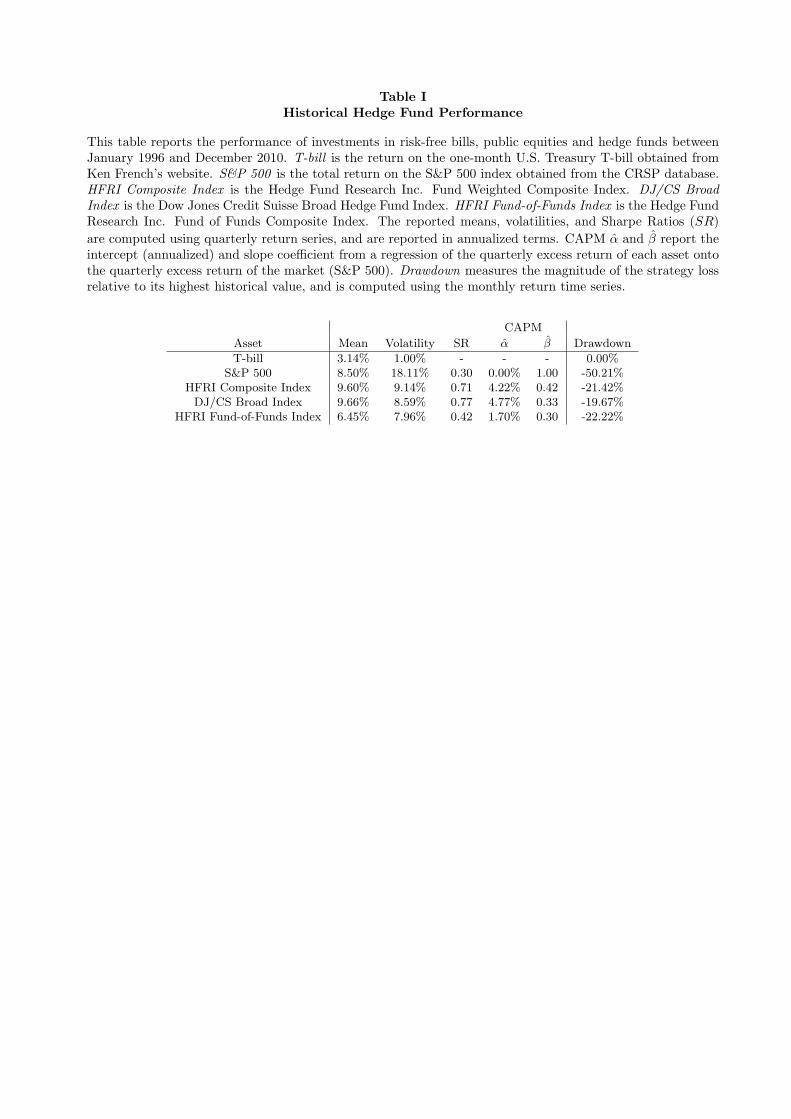
Table IHistorical Hedge Fund Performance

This table reports the performance of investments in risk-free bills, public equities and hedge funds betweenJanuary 1996 and December 2010. T-bill is the return on the one-month U.S. Treasury T-bill obtained fromKen French’s website. S&P 500 is the total return on the S&P 500 index obtained from the CRSP database.HFRI Composite Index is the Hedge Fund Research Inc. Fund Weighted Composite Index. DJ/CS BroadIndex is the Dow Jones Credit Suisse Broad Hedge Fund Index. HFRI Fund-of-Funds Index is the Hedge FundResearch Inc. Fund of Funds Composite Index. The reported means, volatilities, and Sharpe Ratios (SR)

are computed using quarterly return series, and are reported in annualized terms. CAPM α and β report theintercept (annualized) and slope coefficient from a regression of the quarterly excess return of each asset ontothe quarterly excess return of the market (S&P 500). Drawdown measures the magnitude of the strategy lossrelative to its highest historical value, and is computed using the monthly return time series.

CAPM

Asset Mean Volatility SR α β Drawdown

T-bill 3.14% 1.00% - - - 0.00%S&P 500 8.50% 18.11% 0.30 0.00% 1.00 -50.21%

HFRI Composite Index 9.60% 9.14% 0.71 4.22% 0.42 -21.42%DJ/CS Broad Index 9.66% 8.59% 0.77 4.77% 0.33 -19.67%

HFRI Fund-of-Funds Index 6.45% 7.96% 0.42 1.70% 0.30 -22.22%

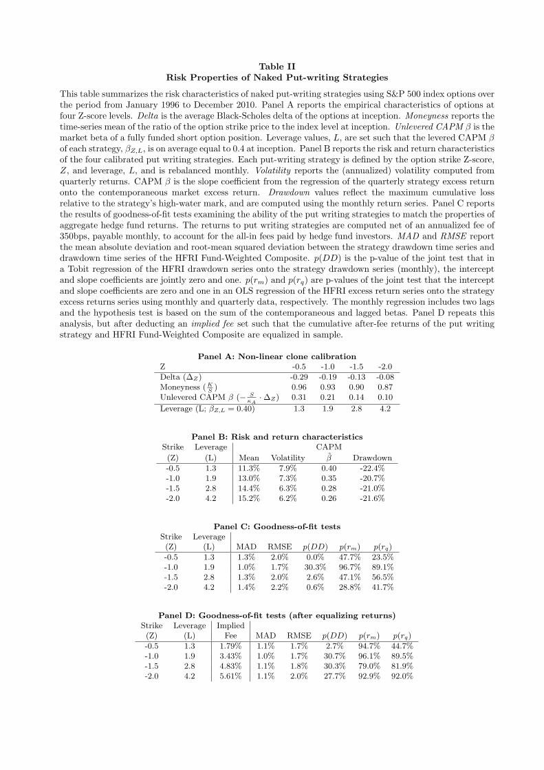
Table IIRisk Properties of Naked Put-writing Strategies

This table summarizes the risk characteristics of naked put-writing strategies using S&P 500 index options overthe period from January 1996 to December 2010. Panel A reports the empirical characteristics of options atfour Z-score levels. Delta is the average Black-Scholes delta of the options at inception. Moneyness reports thetime-series mean of the ratio of the option strike price to the index level at inception. Unlevered CAPM β is themarket beta of a fully funded short option position. Leverage values, L, are set such that the levered CAPM βof each strategy, βZ,L, is on average equal to 0.4 at inception. Panel B reports the risk and return characteristicsof the four calibrated put writing strategies. Each put-writing strategy is defined by the option strike Z-score,Z, and leverage, L, and is rebalanced monthly. Volatility reports the (annualized) volatility computed fromquarterly returns. CAPM β is the slope coefficient from the regression of the quarterly strategy excess returnonto the contemporaneous market excess return. Drawdown values reflect the maximum cumulative lossrelative to the strategy’s high-water mark, and are computed using the monthly return series. Panel C reportsthe results of goodness-of-fit tests examining the ability of the put writing strategies to match the properties ofaggregate hedge fund returns. The returns to put writing strategies are computed net of an annualized fee of350bps, payable monthly, to account for the all-in fees paid by hedge fund investors. MAD and RMSE reportthe mean absolute deviation and root-mean squared deviation between the strategy drawdown time series anddrawdown time series of the HFRI Fund-Weighted Composite. p(DD) is the p-value of the joint test that ina Tobit regression of the HFRI drawdown series onto the strategy drawdown series (monthly), the interceptand slope coefficients are jointly zero and one. p(rm) and p(rq) are p-values of the joint test that the interceptand slope coefficients are zero and one in an OLS regression of the HFRI excess return series onto the strategyexcess returns series using monthly and quarterly data, respectively. The monthly regression includes two lagsand the hypothesis test is based on the sum of the contemporaneous and lagged betas. Panel D repeats thisanalysis, but after deducting an implied fee set such that the cumulative after-fee returns of the put writingstrategy and HFRI Fund-Weighted Composite are equalized in sample.

Panel A: Non-linear clone calibrationZ -0.5 -1.0 -1.5 -2.0

Delta (∆Z) -0.29 -0.19 -0.13 -0.08Moneyness (K

S) 0.96 0.93 0.90 0.87

Unlevered CAPM β (− SκA

·∆Z) 0.31 0.21 0.14 0.10

Leverage (L; βZ,L = 0.40) 1.3 1.9 2.8 4.2

Panel B: Risk and return characteristicsStrike Leverage CAPM

(Z) (L) Mean Volatility β Drawdown

-0.5 1.3 11.3% 7.9% 0.40 -22.4%-1.0 1.9 13.0% 7.3% 0.35 -20.7%-1.5 2.8 14.4% 6.3% 0.28 -21.0%-2.0 4.2 15.2% 6.2% 0.26 -21.6%

Panel C: Goodness-of-fit testsStrike Leverage(Z) (L) MAD RMSE p(DD) p(rm) p(rq)

-0.5 1.3 1.3% 2.0% 0.0% 47.7% 23.5%-1.0 1.9 1.0% 1.7% 30.3% 96.7% 89.1%-1.5 2.8 1.3% 2.0% 2.6% 47.1% 56.5%-2.0 4.2 1.4% 2.2% 0.6% 28.8% 41.7%

Panel D: Goodness-of-fit tests (after equalizing returns)Strike Leverage Implied(Z) (L) Fee MAD RMSE p(DD) p(rm) p(rq)

-0.5 1.3 1.79% 1.1% 1.7% 2.7% 94.7% 44.7%-1.0 1.9 3.43% 1.0% 1.7% 30.7% 96.1% 89.5%-1.5 2.8 4.83% 1.1% 1.8% 30.3% 79.0% 81.9%-2.0 4.2 5.61% 1.1% 2.0% 27.7% 92.9% 92.0%

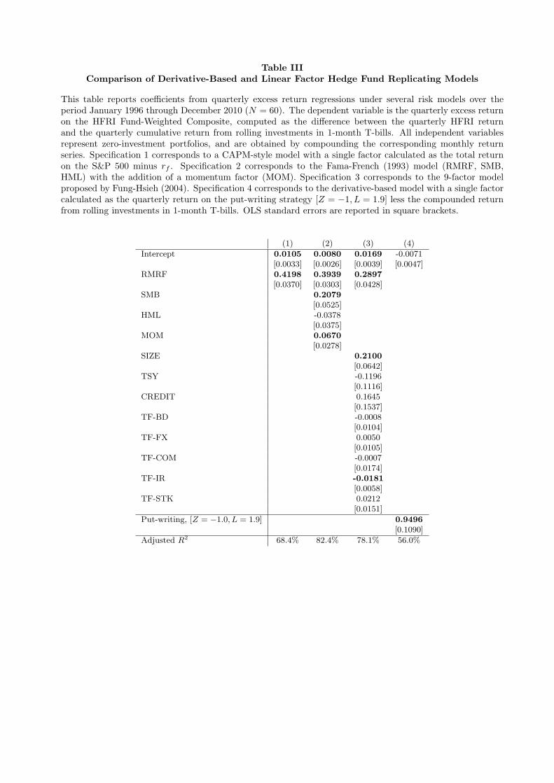
Table IIIComparison of Derivative-Based and Linear Factor Hedge Fund Replicating Models

This table reports coefficients from quarterly excess return regressions under several risk models over theperiod January 1996 through December 2010 (N = 60). The dependent variable is the quarterly excess returnon the HFRI Fund-Weighted Composite, computed as the difference between the quarterly HFRI returnand the quarterly cumulative return from rolling investments in 1-month T-bills. All independent variablesrepresent zero-investment portfolios, and are obtained by compounding the corresponding monthly returnseries. Specification 1 corresponds to a CAPM-style model with a single factor calculated as the total returnon the S&P 500 minus rf . Specification 2 corresponds to the Fama-French (1993) model (RMRF, SMB,HML) with the addition of a momentum factor (MOM). Specification 3 corresponds to the 9-factor modelproposed by Fung-Hsieh (2004). Specification 4 corresponds to the derivative-based model with a single factorcalculated as the quarterly return on the put-writing strategy [Z = −1, L = 1.9] less the compounded returnfrom rolling investments in 1-month T-bills. OLS standard errors are reported in square brackets.

(1) (2) (3) (4)

Intercept 0.0105 0.0080 0.0169 -0.0071[0.0033] [0.0026] [0.0039] [0.0047]

RMRF 0.4198 0.3939 0.2897[0.0370] [0.0303] [0.0428]

SMB 0.2079[0.0525]

HML -0.0378[0.0375]

MOM 0.0670[0.0278]

SIZE 0.2100[0.0642]

TSY -0.1196[0.1116]

CREDIT 0.1645[0.1537]

TF-BD -0.0008[0.0104]

TF-FX 0.0050[0.0105]

TF-COM -0.0007[0.0174]

TF-IR -0.0181[0.0058]

TF-STK 0.0212[0.0151]

Put-writing, [Z = −1.0, L = 1.9] 0.9496[0.1090]

Adjusted R2 68.4% 82.4% 78.1% 56.0%

Table IVReplicating Strategy Comparison

This table reports the goodness-of-fit statistics for tests comparing the monthly drawdown time series of theHFRI Fund-Weighted Composite and various replicating strategies. MAD and RMSE report the mean ab-solute deviation and root-mean squared deviation between the strategy drawdown time series and drawdowntime series of the HFRI Fund-Weighted Composite. Intercept and Slope report the results of a Tobit regres-sion (dependent variable censored above at zero) of the HFRI drawdown series onto the replicating strategydrawdown series, with coefficient standard errors in brackets below. p(DD) is the p-value of the joint testthat the intercept and slope are equal to zero and one, respectively. LL reports the log-likelihood statistic foreach specification.

Replicating strategy MAD RMSE Intercept Slope p(DD) LL

CAPM 2.72% 4.25% 0.0263 0.7755 0.0001 123.48(1 factor) [0.0055] [0.0550]

CAPM with alpha 1.41% 2.33% 0.0104 1.3307 0.0001 159.13(1 factor + intercept) [0.0036] [0.0766]

Fama-French 2.09% 3.35% 0.0305 0.9845 0.0001 149.71(4 factors) [0.0052] [0.0576]

Fama-French with alpha 1.28% 2.25% 0.0176 1.4181 0.0001 173.93(4 factors + intercept) [0.0039] [0.0713]

Fung-Hsieh 3.32% 5.52% 0.0243 0.6139 0.0001 147.13(9 factors) [0.0047] [0.0351]

Fung-Hsieh with alpha 0.90% 1.53% 0.0045 1.1305 0.0030 198.03(9 factors + intercept) [0.0022] [0.0457]

Put-writing, [Z = −1.0, L = 1.9] 1.34% 2.14% 0.0012 1.1677 0.0082 163.69[0.0027] [0.0551]

Put-writing, [Z = −1.0, L = 1.9] 1.02% 1.69% 0.0032 1.0440 0.3029 183.21(- 350bps fee) [0.0024] [0.0458]

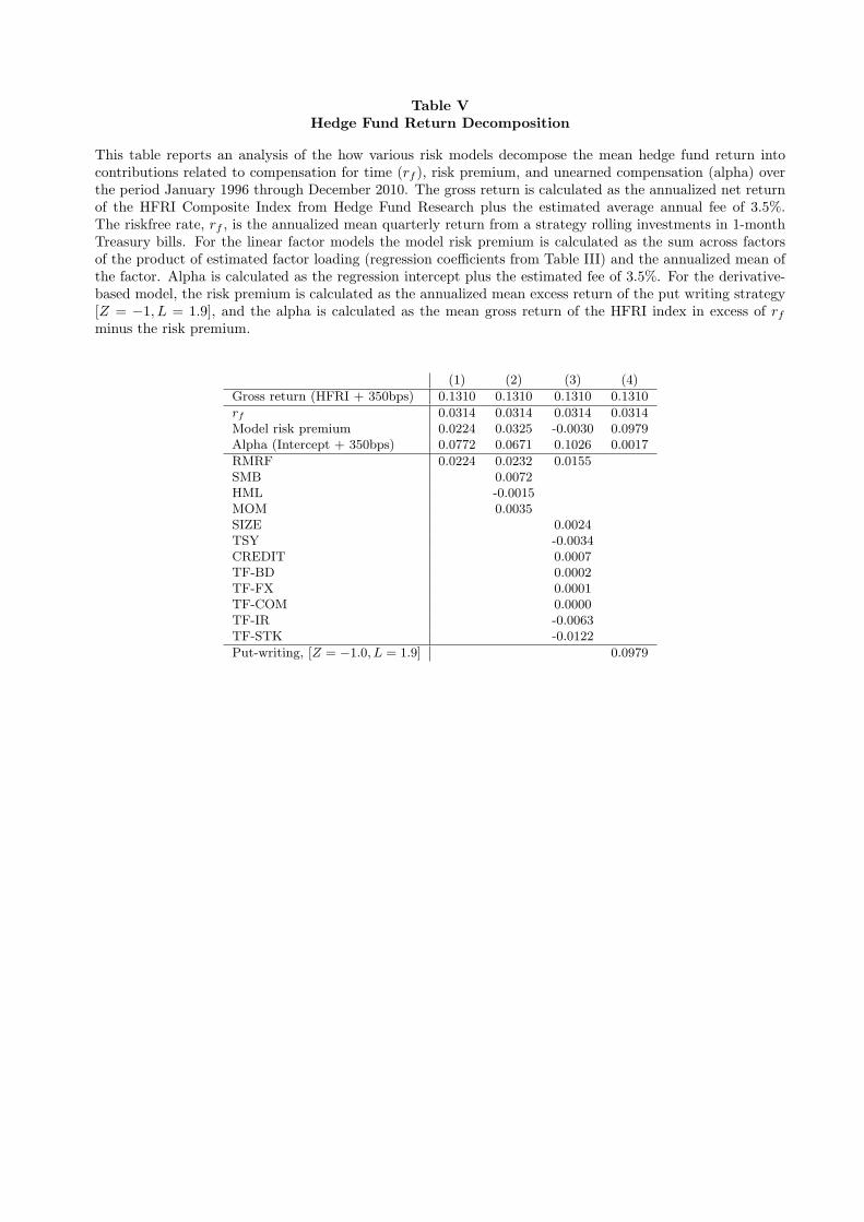
Table VHedge Fund Return Decomposition

This table reports an analysis of the how various risk models decompose the mean hedge fund return intocontributions related to compensation for time (rf ), risk premium, and unearned compensation (alpha) overthe period January 1996 through December 2010. The gross return is calculated as the annualized net returnof the HFRI Composite Index from Hedge Fund Research plus the estimated average annual fee of 3.5%.The riskfree rate, rf , is the annualized mean quarterly return from a strategy rolling investments in 1-monthTreasury bills. For the linear factor models the model risk premium is calculated as the sum across factorsof the product of estimated factor loading (regression coefficients from Table III) and the annualized mean ofthe factor. Alpha is calculated as the regression intercept plus the estimated fee of 3.5%. For the derivative-based model, the risk premium is calculated as the annualized mean excess return of the put writing strategy[Z = −1, L = 1.9], and the alpha is calculated as the mean gross return of the HFRI index in excess of rfminus the risk premium.

(1) (2) (3) (4)

Gross return (HFRI + 350bps) 0.1310 0.1310 0.1310 0.1310

rf 0.0314 0.0314 0.0314 0.0314Model risk premium 0.0224 0.0325 -0.0030 0.0979Alpha (Intercept + 350bps) 0.0772 0.0671 0.1026 0.0017

RMRF 0.0224 0.0232 0.0155SMB 0.0072HML -0.0015MOM 0.0035SIZE 0.0024TSY -0.0034CREDIT 0.0007TF-BD 0.0002TF-FX 0.0001TF-COM 0.0000TF-IR -0.0063TF-STK -0.0122

Put-writing, [Z = −1.0, L = 1.9] 0.0979

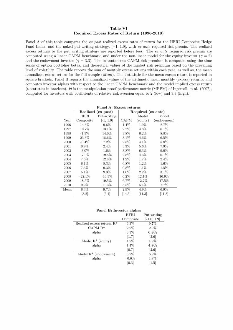
Table VIRequired Excess Rates of Return (1996-2010)

Panel A of this table compares the ex post realized excess rates of return for the HFRI Composite HedgeFund Index, and the naked put-writing strategy, [−1, 1.9], with ex ante required risk premia. The realizedexcess returns to the put writing strategy are reported before fees. The ex ante required risk premia arecomputed using a linear CAPM benchmark, and under the non-linear model for the equity investor (γ = 2)and the endowment investor (γ = 3.3). The instantaneous CAPM risk premium is computed using the timeseries of option portfolios betas, and theoretical values of the market risk premium based on the prevailinglevel of volatility. The table reports the sum of monthly excess returns within each year, as well as, the meanannualized excess return for the full sample (Mean). The t-statistic for the mean excess return is reported insquare brackets. Panel B reports the annualized values of the arithmetic mean monthly (excess) returns, andcomputes investor alphas with respect to the linear CAPM benchmark and the model implied excess return(t-statistics in brackets). Θ is the manipulation-proof performance metric (MPPM) of Ingersoll, et al. (2007),computed for investors with coefficients of relative risk aversion equal to 2 (low) and 3.3 (high).

Panel A: Excess returnsRealized (ex post) Required (ex ante)HFRI Put-writing Model Model

Year Composite [-1, 1.9] CAPM (equity) (endowment)

1996 14.3% 9.6% 1.4% 1.9% 2.7%1997 10.7% 13.1% 2.7% 4.3% 6.1%1998 -1.5% 14.0% 3.8% 6.2% 8.8%1999 23.3% 18.6% 3.1% 4.6% 6.5%2000 -0.4% 7.2% 2.5% 4.1% 5.8%2001 0.9% 2.4% 3.3% 5.6% 7.9%2002 -3.0% 1.6% 3.8% 6.3% 9.0%2003 17.0% 19.5% 2.8% 4.3% 6.1%2004 7.6% 12.8% 1.2% 1.7% 2.4%2005 6.1% 8.3% 0.8% 1.2% 1.6%2006 7.6% 9.3% 0.8% 1.1% 1.5%2007 5.1% 9.3% 1.6% 2.2% 3.1%2008 -22.1% -10.3% 6.2% 12.1% 16.9%2009 18.5% 19.5% 6.7% 12.2% 17.5%2010 9.9% 11.3% 3.5% 5.4% 7.7%

Mean 6.3% 9.7% 2.9% 4.9% 6.9%[3.2] [5.1] [14.5] [11.3] [11.3]

Panel B: Investor alphasHFRI Put writing

Composite [-1.0, 1.9]

Realized excess return, R* 6.3% 9.7%

CAPM R* 2.9% 2.9%alpha 3.3% 6.8%

[1.7] [3.6]

Model R* (equity) 4.9% 4.9%alpha 1.4% 4.9%

[0.7] [2.6]

Model R* (endowment) 6.9% 6.9%alpha -0.6% 1.8%

[0.3] [1.5]

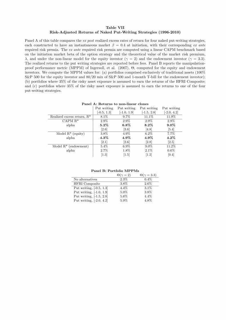
Table VIIRisk-Adjusted Returns of Naked Put-Writing Strategies (1996-2010)

Panel A of this table compares the ex post realized excess rates of return for four naked put-writing strategies,each constructed to have an instantaneous market β = 0.4 at initiation, with their corresponding ex anterequired risk premia. The ex ante required risk premia are computed using a linear CAPM benchmark basedon the initiation market beta of the option strategy and the theoretical value of the market risk premium,λ, and under the non-linear model for the equity investor (γ = 2) and the endowment investor (γ = 3.3).The realized returns to the put writing strategies are reported before fees. Panel B reports the manipulation-proof performance metric (MPPM) of Ingersoll, et al. (2007), Θ, computed for the equity and endowmentinvestors. We compute the MPPM values for: (a) portfolios comprised exclusively of traditional assets (100%S&P 500 for the equity investor and 80/20 mix of S&P 500 and 1-month T-bill for the endowment investor);(b) portfolios where 35% of the risky asset exposure is assumed to earn the returns of the HFRI Composite;and (c) portfolios where 35% of the risky asset exposure is assumed to earn the returns to one of the fourput-writing strategies.

Panel A: Returns to non-linear clonesPut writing Put writing Put writing Put writing[-0.5, 1.3] [-1.0, 1.9] [-1.5, 2.8] [-2.0, 4.2]

Realized excess return, R* 8.1% 9.7% 11.1% 11.9%

CAPM R* 2.9% 2.9% 2.9% 2.9%alpha 5.2% 6.8% 8.2% 9.0%

[2.6] [3.6] [4.8] [5.4]

Model R* (equity) 3.8% 4.9% 6.2% 7.7%alpha 4.3% 4.9% 4.9% 4.2%

[2.1] [2.6] [2.8] [2.5]

Model R* (endowment) 5.4% 6.9% 9.0% 11.2%alpha 2.7% 1.8% 2.1% 0.6%

[1.3] [1.5] [1.2] [0.4]

Panel B: Portfolio MPPMsΘ(γ = 2) Θ(γ = 3.3)

No alternatives 2.3% 0.4%

HFRI Composite 3.8% 2.6%

Put writing, [-0.5, 1.3] 4.4% 3.1%Put writing, [-1.0, 1.9] 5.0% 3.8%Put writing, [-1.5, 2.8] 5.6% 4.4%Put writing, [-2.0, 4.2] 5.9% 4.8%

Figure 1. Asset Class Performance Comparison. This figure plots the total return indices for two hedgefund indices – the Hedge Fund Research Inc. (HFRI) Fund Weighted Composite Index, and the Dow JonesCredit Suisse Broad Hedge Fund Index – the HFRI Fund-of-Funds Composite Index, the S&P 500 Index, anda strategy that rolls over one-month U.S. Treasury bills over the period from January 1996 to December 2010(N = 180 months).

Jul97 Jan00 Jul02 Jan05 Jul07 Jan101

1.5

2

2.5

3

3.5

4

HFRI Composite IndexDJ/CS Broad IndexHFRI Fund−of−Funds IndexS&P 500T−bill

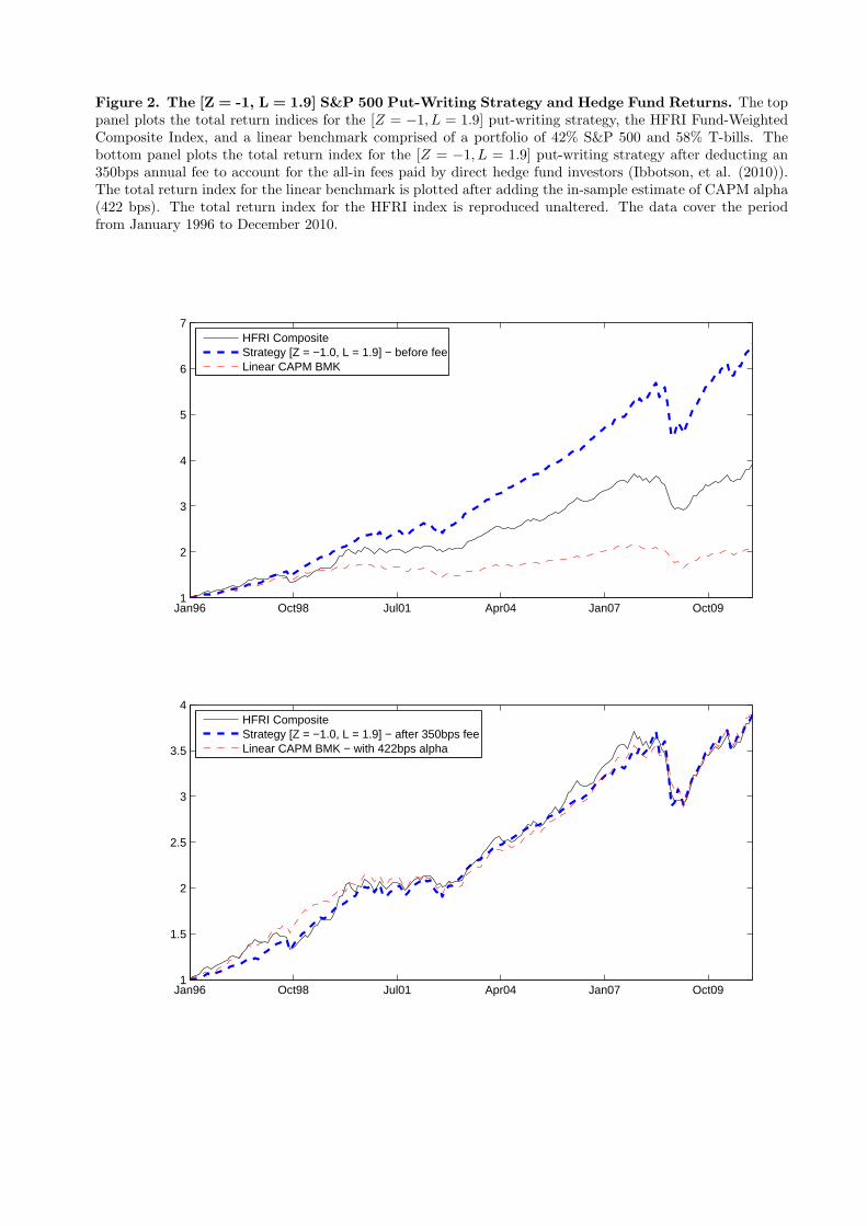
Figure 2. The [Z = -1, L = 1.9] S&P 500 Put-Writing Strategy and Hedge Fund Returns. The toppanel plots the total return indices for the [Z = −1, L = 1.9] put-writing strategy, the HFRI Fund-WeightedComposite Index, and a linear benchmark comprised of a portfolio of 42% S&P 500 and 58% T-bills. Thebottom panel plots the total return index for the [Z = −1, L = 1.9] put-writing strategy after deducting an350bps annual fee to account for the all-in fees paid by direct hedge fund investors (Ibbotson, et al. (2010)).The total return index for the linear benchmark is plotted after adding the in-sample estimate of CAPM alpha(422 bps). The total return index for the HFRI index is reproduced unaltered. The data cover the periodfrom January 1996 to December 2010.

Jan96 Oct98 Jul01 Apr04 Jan07 Oct091

2

3

4

5

6

7

HFRI CompositeStrategy [Z = −1.0, L = 1.9] − before feeLinear CAPM BMK

Jan96 Oct98 Jul01 Apr04 Jan07 Oct091

1.5

2

2.5

3

3.5

4

HFRI CompositeStrategy [Z = −1.0, L = 1.9] − after 350bps feeLinear CAPM BMK − with 422bps alpha

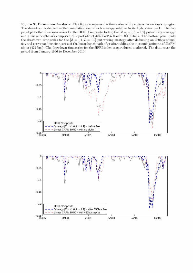
Figure 3. Drawdown Analysis. This figure compares the time series of drawdowns on various strategies.The drawdown is defined as the cumulative loss of each strategy relative to its high water mark. The toppanel plots the drawdown series for the HFRI Composite Index, the [Z = −1, L = 1.9] put-writing strategy,and a linear benchmark comprised of a portfolio of 42% S&P 500 and 58% T-bills. The bottom panel plotsthe drawdown time series for the [Z = −1, L = 1.9] put-writing strategy after deducting an 350bps annualfee, and corresponding time series of the linear benchmark after after adding the in-sample estimate of CAPMalpha (422 bps). The drawdown time series for the HFRI index is reproduced unaltered. The data cover theperiod from January 1996 to December 2010.

Jan96 Oct98 Jul01 Apr04 Jan07 Oct09−0.25

−0.2

−0.15

−0.1

−0.05

0

HFRI CompositeStrategy [Z = −1.0, L = 1.9] − before feeLinear CAPM BMK − with no alpha

Jan96 Oct98 Jul01 Apr04 Jan07 Oct09−0.25

−0.2

−0.15

−0.1

−0.05

0

HFRI CompositeStrategy [Z = −1.0, L = 1.9] − after 350bps feeLinear CAPM BMK − with 422bps alpha

Figure 4. The Cost of Capital for Risky Assets. The following figure displays the investor’s cost ofcapital as a function of his allocation to the the risky asset. The left (right) panel illustrates the case of a shiftin the allocation from the risk free asset into the equity index (non-linear hedge fund clone) for the equityinvestor (γ = 2) and an endowment investor (γ = 3.3). The state-contingent payoff profile of the aggregatehedge fund universe is assumed to be described by our non-linear clone, the [Z = −1, L = 1.9] put-writingstrategy. Proper is the model-implied cost of capital at the given allocation; Linear is the cost-of-capitalcomputed under a linear mean-variance rule.

0 0.2 0.4 0.6 0.8 10

0.05

0.1

0.15Equity index [β = 1.0]

Inve

stor

req

uire

d ex

cess

rat

e of

ret

urn

Share of portfolio in risky asset

0 0.2 0.4 0.6 0.8 10

0.05

0.1

0.15Alternative: [Z = −1.0, L = 1.9]

Inve

stor

req

uire

d ex

cess

rat

e of

ret

urn

Share of portfolio in risky asset

Proper: γ = 2.0Linear: γ = 2.0Proper: γ = 3.3Linear: γ = 3.3

Proper: γ = 2.0Linear: γ = 2.0Proper: γ = 3.3Linear: γ = 3.3

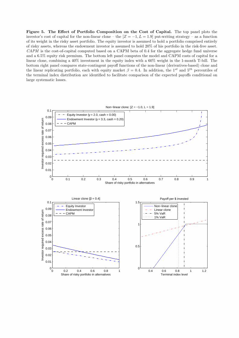
Figure 5. The Effect of Portfolio Composition on the Cost of Capital. The top panel plots theinvestor’s cost of capital for the non-linear clone – the [Z = −1, L = 1.9] put-writing strategy – as a functionof its weight in the risky asset portfolio. The equity investor is assumed to hold a portfolio comprised entirelyof risky assets, whereas the endowment investor is assumed to hold 20% of his portfolio in the risk-free asset.CAPM is the cost-of-capital computed based on a CAPM beta of 0.4 for the aggregate hedge fund universeand a 6.5% equity risk premium. The bottom left panel computes the model and CAPM costs of capital for alinear clone, combining a 40% investment in the equity index with a 60% weight in the 1-month T-bill. Thebottom right panel compares state-contingent payoff functions of the non-linear (derivatives-based) clone andthe linear replicating portfolio, each with equity market β = 0.4. In addition, the 1st and 5th percentiles ofthe terminal index distribution are identified to facilitate comparison of the expected payoffs conditional onlarge systematic losses.

0.4 0.6 0.8 1 1.20

0.5

1

1.5Payoff per $ invested

Terminal index level

0 0.2 0.4 0.6 0.8 10

0.01

0.02

0.03

0.04

0.05

0.06

0.07

0.08

0.09

0.1

Inve

stor

req

uire

d ex

cess

rat

e of

ret

urn

Share of risky portfolio in alternatives

Linear clone [β = 0.4]

0 0.1 0.2 0.3 0.4 0.5 0.6 0.7 0.8 0.9 10

0.01

0.02

0.03

0.04

0.05

0.06

0.07

0.08

0.09

0.1

Inve

stor

req

uire

d ex

cess

rat

e of

ret

urn

Share of risky portfolio in alternatives

Non−linear clone: [Z = −1.0, L = 1.9]

Equity InvestorEndowment InvestorCAPM

Equity Investor (γ = 2.0, cash = 0.00)

Endowment Investor (γ = 3.3, cash = 0.20)CAPM

Non−linear cloneLinear clone5% VaR1% VaR

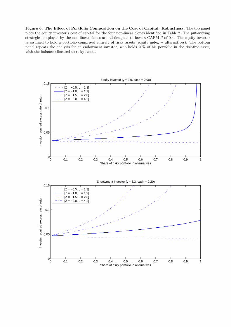
Figure 6. The Effect of Portfolio Composition on the Cost of Capital: Robustness. The top panelplots the equity investor’s cost of capital for the four non-linear clones identified in Table 2. The put-writingstrategies employed by the non-linear clones are all designed to have a CAPM β of 0.4. The equity investoris assumed to hold a portfolio comprised entirely of risky assets (equity index + alternatives). The bottompanel repeats the analysis for an endowment investor, who holds 20% of his portfolio in the risk-free asset,with the balance allocated to risky assets.

0 0.1 0.2 0.3 0.4 0.5 0.6 0.7 0.8 0.9 10

0.05

0.1

0.15

Share of risky portfolio in alternatives

Inve

stor

req

uire

d ex

cess

rat

e of

ret

urn

Equity Investor (γ = 2.0, cash = 0.00)

0 0.1 0.2 0.3 0.4 0.5 0.6 0.7 0.8 0.9 10

0.05

0.1

0.15

Share of risky portfolio in alternatives

Inve

stor

req

uire

d ex

cess

rat

e of

ret

urn

Endowment Investor (γ = 3.3, cash = 0.20)

[Z = −0.5, L = 1.3][Z = −1.0, L = 1.9][Z = −1.5, L = 2.8][Z = −2.0, L = 4.2]

[Z = −0.5, L = 1.3][Z = −1.0, L = 1.9][Z = −1.5, L = 2.8][Z = −2.0, L = 4.2]

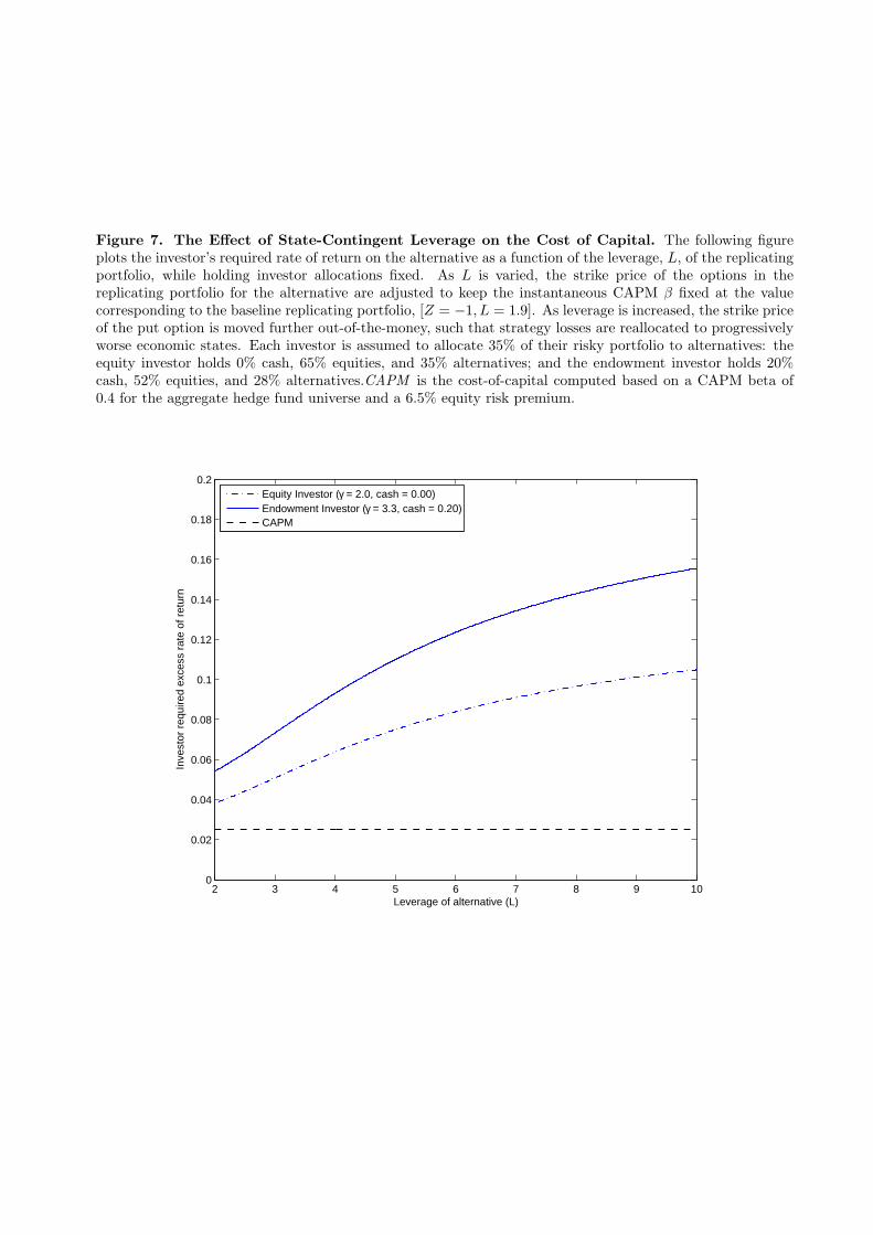
Figure 7. The Effect of State-Contingent Leverage on the Cost of Capital. The following figureplots the investor’s required rate of return on the alternative as a function of the leverage, L, of the replicatingportfolio, while holding investor allocations fixed. As L is varied, the strike price of the options in thereplicating portfolio for the alternative are adjusted to keep the instantaneous CAPM β fixed at the valuecorresponding to the baseline replicating portfolio, [Z = −1, L = 1.9]. As leverage is increased, the strike priceof the put option is moved further out-of-the-money, such that strategy losses are reallocated to progressivelyworse economic states. Each investor is assumed to allocate 35% of their risky portfolio to alternatives: theequity investor holds 0% cash, 65% equities, and 35% alternatives; and the endowment investor holds 20%cash, 52% equities, and 28% alternatives.CAPM is the cost-of-capital computed based on a CAPM beta of0.4 for the aggregate hedge fund universe and a 6.5% equity risk premium.

2 3 4 5 6 7 8 9 100

0.02

0.04

0.06

0.08

0.1

0.12

0.14

0.16

0.18

0.2

Inve

stor

req

uire

d ex

cess

rat

e of

ret

urn

Leverage of alternative (L)

Equity Investor (γ = 2.0, cash = 0.00)Endowment Investor (γ = 3.3, cash = 0.20)CAPM

Figure 8. Required Rate of Return for Hedge Funds Through Time. The following figure plots therequired rate of return for the hedge fund replicating strategy ([Z = −1, L = 1.9]) through time for the equityinvestor (γ = 2) and the endowment investor (γ = 3.3). Each investor is assumed to allocate 35% of theirrisky portfolio to alternatives: the equity investor holds 0% cash, 65% equities, and 35% alternatives; and theendowment investor holds 20% cash, 52% equities, and 28% alternatives. The equity return volatility, σ, usedto compute the required rate of return for month t is set equal to 0.8 of the implied volatility (VIX) index onthe last business day of the preceding month. The skewness and kurtosis of the parameterized normal inverseGaussian (NIG) distribution are held fixed at the baseline values.

Jul97 Jan00 Jul02 Jan05 Jul07 Jan100

0.1

0.2

0.3

0.4

0.5

0.6

0.7Non−linear clone: [Z = −1.0, L = 1.9]

Inve

stor

req

uire

d ex

cess

rat

e of

ret

urn

Equity Investor (γ = 2.0)Endowment Investor (γ = 3.3)

Figure 9. Declining Allocations to Assets with Increasing CAPM α’s. This figure illustrates theproper portfolio allocations, as a function of investor risk aversion, γ, to three alternative strategies that grouplosses in progressively worse economic states by increasing the leverage factors (higher L values), while makingthe underlying assets safer (more negative Z values). The strategies are designed to have constant CAPM β’sequal to 0.4, and offer an increasing sequence of CAPM α’s of 4% (left panel), 5% (center panel), and 6%(right panel).

2 3 4 50

0.1

0.2

0.3

0.4

0.5

0.6

0.7

0.8

0.9

1

Risk aversion (γ)

Por

tfolio

sha

re

[Z = −0.9, L = 2.0]

Risk−freeEquityAlternative

2 3 4 50

0.1

0.2

0.3

0.4

0.5

0.6

0.7

0.8

0.9

1

Risk aversion (γ)

Por

tfolio

sha

re

[Z = −1.6, L = 4.0]

Risk−freeEquityAlternative

2 3 4 50

0.1

0.2

0.3

0.4

0.5

0.6

0.7

0.8

0.9

1

Risk aversion (γ)

Por

tfolio

sha

re

[Z = −2.2, L = 10.0]

Risk−freeEquityAlternative