the control of interior cabin noise due - virginia tech
TRANSCRIPT
THE CONTROL OF INTERIOR CABIN NOISE DUE TO A TURBULENT
BOUNDARY LAYER NOISE EXCITATION USING SMART FOAM ELEMENTS
by Jason R. Griffin
Thesis submitted to the Faculty of the Virginia Polytechnic Institute and State University
in partial fulfillment of the requirements for the degree of
Masters of Science in
Mechanical Engineering
Dr. Chris R. Fuller, Chairman Dr. Ricardo A. Burdisso Dr. Martin E. Johnson
May 2006 Blacksburg, Virginia
Keywords: Smart Foam, Active noise control, Passive noise control, Interior cabin noise, Turbulent Boundary Layer
THE CONTROL OF INTERIOR CABIN NOISE DUE TO A TURBULENT
BOUNDARY LAYER NOISE EXCITATION USING SMART FOAM ELEMENTS
By Jason R. Griffin
Committee Chairman: Chris R. Fuller, Mechanical Engineering
(ABSTRACT)
In this work, the potential for a smart foam actuator in controlling interior cabin noise due
to a turbulent boundary layer excitation has been experimentally demonstrated. A smart
foam actuator is a device comprised of sound absorbing foam with an embedded
distributed piezoelectric layer (PVDF) designed to operate over a broad range of
frequencies. The acoustic foam acts as a passive absorber and targets the high frequency
content, while the PVDF serves as the active component and is used to overcome the
limitations of the acoustic foam at low frequencies. The fuselage skin of an aircraft was
represented by an experimental test panel in an anechoic box mounted to the side of a
wind tunnel. The rig was used to simulate turbulent boundary layer noise transmission
into and aircraft cabin. An active noise control (ANC) methodology was employed by
covering the test panel with the smart foam actuators and driving them to generate a
secondary sound field. This secondary sound field, when superimposed with the panel
radiation, resulted in a reduction in overall sound in the anechoic box. An adaptive
feedforward filtered-x Least-Mean-Squared (LMS) control algorithm was used to drive
the smart foam actuators to reduce the sound pressure levels at an array of microphones.
Accelerometers measured the response of the test panel and were used as the reference
signal for the feedforward algorithm. A detailed summary of the smart foam actuator
control performance is presented for two separate low speed wind tunnel facilities with
speeds of Mach 0.1 and Mach 0.2 and a single high speed tunnel facility operating at
Mach 0.8 and Mach 2.5.
iii
Acknowledgements
I would like to thank my research advisor, Dr. Chris R. Fuller, for giving me the
opportunity to explore the field of acoustics and for guiding me throughout the course of
my project. I also must thank Dr. Ricardo A. Burdisso and Dr. Marty E. Johnson for
serving on my advisory committee. I must express a deep gratitude to Marty for all the
effort that he put forth on my behalf. I appreciate the expert guidance he provided when
helping me conduct experiments, his patience with my lack of understanding, and his
enthusiasm for knowledge, particularly in the field of acoustics.
I am indebted to NASA Langley Research Center for funding this work. I would
like to thank especially Dr. Gary Gibbs and Dr. Richard Silcox for their efforts in
coordinating various phases of the project.
There are several members of the Vibrations and Acoustics Laboratories team
who have assisted me in various ways. Thanks to Dawn Bennett for her patients and
effort in assisting me with many administrative tasks. Thanks to Steve Booth and Chad
Burchett for helping me build my test rig.
Finally, I would like to express my sincere thanks to my loving wife Denise for
her always positive attitude and words of encouragement in her support of my many
endeavors.
iv
Table of Contents
Chapter 1
Introduction..................................................................................................................... 1
1.1 Aircraft Interior Noise........................................................................................ 1
1.2 Noise Control Techniques.................................................................................. 3
1.3 Control of Aircraft Interior Noise ...................................................................... 5
1.4 Previous Work on Smart Foam.......................................................................... 9
1.5 Organization of Thesis....................................................................................... 13
Chapter 2
Smart Foam Elements .................................................................................................... 14
2.1 Introduction........................................................................................................ 14
2.2 Active Component ............................................................................................. 15
2.3 Passive Component............................................................................................ 17
2.4 Construction....................................................................................................... 18
2.5 Characterization ................................................................................................. 22
2.6 Summary ............................................................................................................ 25
Chapter 3
Control Methodology...................................................................................................... 27
3.1 Introduction........................................................................................................ 27
3.2 Feedforward Filtered-x LMS Algorithm ........................................................... 28
3.2.1 Single Channel Control............................................................................. 28
3.2.2 Multiple Channel Control ......................................................................... 32
TABLE OF CONTENTS v
3.3 Practical Implementation of Control Algorithm................................................ 32
3.3.1 Causality ................................................................................................... 35
3.3.2 Multiple Coherence................................................................................... 36
Chapter 4
Test Methodology and Experimental Components ..................................................... 41
4.1 Introduction........................................................................................................ 41
4.2 VPI Wind Tunnel............................................................................................... 43
4.3 Anechoic Enclosure ........................................................................................... 49
4.3.1 Construction.............................................................................................. 50
4.3.2 Characterization ........................................................................................ 51
4.3.2.1 Reverberation .................................................................................... 52
4.3.2.2 Noise Reduction ................................................................................ 53
Chapter 5
Experimental Results...................................................................................................... 56
5.1 Introduction........................................................................................................ 56
5.2 Acquisition Sensors ........................................................................................... 58
5.3 NASA LaRC Low Speed Experiments.............................................................. 59
5.3.1 Test Panel.................................................................................................. 59
5.3.2 Measurement Setup................................................................................... 61
5.3.2.1 Actuators ........................................................................................... 61
5.3.2.2 Error Microphones ............................................................................ 62
5.3.2.3 Reference Accelerometers................................................................. 63
5.3.2.4 Controller........................................................................................... 65
5.3.2.5 Data Acquisition................................................................................ 66
5.3.3 Results....................................................................................................... 66
5.4 AEDC High Speed Experiments........................................................................ 71
5.4.1 Test Panel.................................................................................................. 71
5.4.2 Measurement Setup................................................................................... 71
5.4.2.1 Actuators ........................................................................................... 71
TABLE OF CONTENTS vi
5.4.2.2 Instrumentation.................................................................................. 73
5.4.2.3 Controller........................................................................................... 74
5.4.2.4 Data Acquisition................................................................................ 76
5.4.3 Results....................................................................................................... 76
5.4.3.1 Mach 0.8............................................................................................ 76
5.4.3.2 Mach 2.5............................................................................................ 79
5.5 VPI Low Speed Experiments............................................................................. 81
5.5.1 Test Panel.................................................................................................. 81
5.5.2 Measurement Setup................................................................................... 81
5.5.2.1 Actuators ........................................................................................... 81
5.5.2.2 Instrumentation.................................................................................. 82
5.5.2.3 Control and Data Acquisition............................................................ 83
5.5.3 Results....................................................................................................... 84
Chapter 6
Conclusions and Future Work....................................................................................... 89
Bibliography .................................................................................................................... 92
Appendix
Test Panel Mode Shapes................................................................................................. 97
Vita ...................................................................................................................................102

vii
List of Figures Figure 2.1 Numerical classification of PVDF axes....................................................... 16
Figure 2.2 (a) Deformation of PVDF. (b) Translation of PVDF into useful motion .... 19
Figure 2.3 (a) Components of a smart foam element. (b) Smart foam element
mounted to a structure.................................................................................. 20
Figure 2.4 Smart foam element ..................................................................................... 21
Figure 2.5 (a) PVDF with free boundary conditions. (b) PVDF with fixed boundary
conditions..................................................................................................... 22
Figure 2.6 Two plate mode shapes Ψmn. (a) Ψ11 with a single actuator. (b) Ψ21 with
multiple actuators......................................................................................... 23
Figure 2.7 Ten microphone hemispherical array........................................................... 24
Figure 2.8 (a) Original smart foam element configuration. (b) Modified smart foam
element configuration .................................................................................. 25
Figure 2.9 (a) Radiation characteristics of a smart foam element. (b) Increase in
sound power radiation due to smart foam improvments.............................. 26
Figure 3.1 Block diagram of single channel Filtered-x LMS feedforward control
system .......................................................................................................... 28
Figure 3.2 Single-input adaptive FIR filter where output is the weighted sum of past
input values .................................................................................................. 30
Figure 3.3 Block diagram of MIMO control setup ....................................................... 34
Figure 3.4 (a) Ordinary coherence function between one reference sensor and one
error. (b) Estimate of active control based on coherence............................. 39
Figure 3.5 (a) Ordinary coherence function between four reference sensors and one
error. (b) Estimate of active control based on coherence .............................. 40
Figure 4.1 Schematic of interior noise control using smart foam actuators.................. 41
LIST OF FIGURES viii
Figure 4.2 Schematic of experimental methodology..................................................... 42
Figure 4.3 VPI wind tunnel configuration..................................................................... 44
Figure 4.4 Experimental demonstration of duct cut-on frequency................................ 44
Figure 4.5 VPI wind tunnel noise characteristics.......................................................... 46
Figure 4.6 Duct coherence between microphones 2 in. horizontally spaced ................ 46
Figure 4.7 VPI test panel accelerometer response characteristics................................. 47
Figure 4.8 VPI plate coherence between accelerometers 2 in. apart............................. 47
Figure 4.9 VPI wind tunnel noise characteristics.......................................................... 48
Figure 4.10 VPI wind tunnel test facility ........................................................................ 49
Figure 4.11 Anechoic enclosure...................................................................................... 51
Figure 4.12 Resonant behavior of anechoic enclosure.................................................... 53
Figure 4.13 Noise reduction of anechoic enclosure. (a) Microphone response. (b)
Noise reduction levels.................................................................................. 55
Figure 5.1 NASA LaRC test panel................................................................................ 59
Figure 5.2 Actuator used in NASA LaRC experiments ................................................ 61
Figure 5.3 NASA LaRC actuator configuration............................................................ 62
Figure 5.4 Multiple coherence of NASA LaRC panel .................................................. 64
Figure 5.5 Schematic of experimental setup ................................................................. 67
Figure 5.6 (a) NASA LaRC six-bay panel with smart foam actuators mounted to test
section. (b) View of reference accelerometer centered on control channel
two................................................................................................................ 67
Figure 5.7 NASA LaRC panel with anechoic enclosure mounted in place .................. 68
Figure 5.8 (a) NASA LaRC results with a control bandwidth of 400-1000 Hz. (b)
Detail view of control bandwidth ................................................................ 69
Figure 5.9 NASA LaRC attenuation results in one-third octave bands ........................ 70
Figure 5.10 AEDC test panel .......................................................................................... 71
Figure 5.11 Actuator used in AEDC experiments........................................................... 72
Figure 5.12 AEDC actuator configuration ...................................................................... 73
Figure 5.13 Multiple coherence of AEDC panel. (a) Mach 0.8 flow speed. (b) Mach
2.5 flow speed .............................................................................................. 75
LIST OF FIGURES ix
Figure 5.14 (a) AEDC Mach 0.8 results with a control bandwidth of 400-800 Hz. (b)
Detail view of control bandwidth ................................................................ 77
Figure 5.15 AEDC Mach 0.8 attenuation results in one-third octave bands................... 78
Figure 5.16 AEDC Mach 2.5 results with a control bandwidth of 400-800 ................... 79
Figure 5.17 AEDC Mach 2.5 attenuation results in one-third octave bands................... 80
Figure 5.18 Actuator used in VPI experiments ............................................................... 83
Figure 5.19 VPI actuator configuration........................................................................... 83
Figure 5.20 Multiple coherence of VPI panel ................................................................. 84
Figure 5.21 (a) VPI results with a control bandwidth of 250-630 Hz. (b) Detail view
of control bandwidth .................................................................................... 85
Figure 5.22 Passive attenuation properties of a smart foam actuator by components .... 86
Figure 5.23 VPI attenuation in one-third octave bands................................................... 88
Figure A.1 Experimental mode shapes of NASA LaRC test panel ............................... 98
Figure A.2 Experimental mode shapes of AEDC test panel .......................................... 99
Figure A.3 Experimental mode shapes of VPI test panel: modes 1-8...........................100
Figure A.4 Experimental mode shapes of VPI test panel: modes 9-12.........................101
x
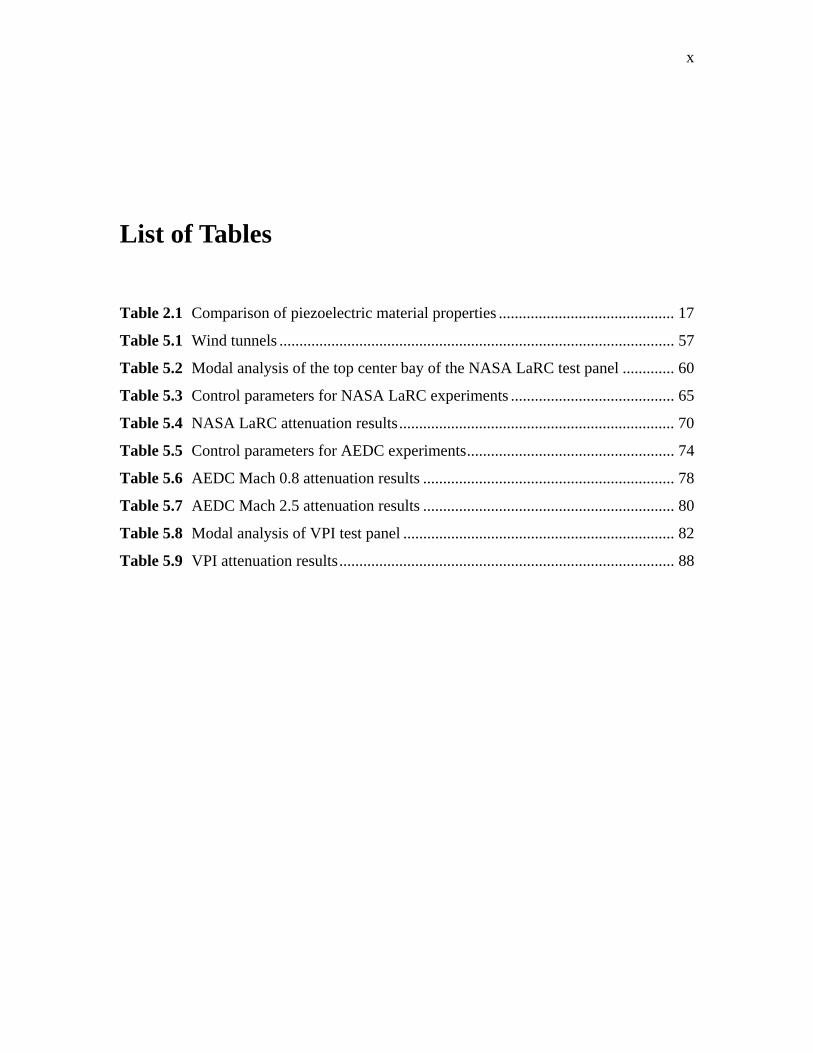
List of Tables Table 2.1 Comparison of piezoelectric material properties ............................................ 17
Table 5.1 Wind tunnels ................................................................................................... 57
Table 5.2 Modal analysis of the top center bay of the NASA LaRC test panel ............. 60
Table 5.3 Control parameters for NASA LaRC experiments ......................................... 65
Table 5.4 NASA LaRC attenuation results..................................................................... 70
Table 5.5 Control parameters for AEDC experiments.................................................... 74
Table 5.6 AEDC Mach 0.8 attenuation results ............................................................... 78
Table 5.7 AEDC Mach 2.5 attenuation results ............................................................... 80
Table 5.8 Modal analysis of VPI test panel .................................................................... 82
Table 5.9 VPI attenuation results.................................................................................... 88

1
Chapter 1 Introduction Mankind since creation has been obsessed with overcoming the physical limitations of
our human bodies to get from one place to another quickly. Automobiles, rail systems,
and aircraft are common transportation methods utilized daily to satisfy the perceived
need we have for constant relocation. Advances in these technologies now make it
possible for individuals to reach almost any destination on earth in a matter of hours and
conduct business during travel. Since travel times have become a significant portion of
each day for many people, recent focus has been directed on maximizing travel comfort.
One such focus has been on controlling the level of background noise present in the
interior cabins of both automobiles and aircraft.
Suppression of an aircraft’s interior noise can be appreciated by anyone who has
spent a long time in continuous flight. Continuous flight subjects both passengers and
crew to constant background noise that can result in communication difficulties and
fatigue. Although this may only create a level of discomfort to passengers, greater
consequences exist should the noise impede a pilot’s ability to communicate and control
the aircraft with maximum efficiency and attentiveness.
1.1 AIRCRAFT INTERIOR NOISE Noise generated by air traffic is a significant byproduct of the world’s growing air
transportation network. Knowing that noise reduction technology is slow to mature, it
was necessary to develop a program plan for the future before a critical need for the
technology existed. Thus the National Aeronautics and Space Administration (NASA),
CHAPTER 1 INTRODUCTION 2
Federal Aviation Administration (FAA), and U.S. industry (manufacturers, operators and
airport/community planners) have developed joint noise reduction technology programs
that have application to virtually all classes of subsonic and supersonic aircraft
envisioned to operate far into the 21st century [1]. The Advanced Subsonic Technology
(AST) noise reduction program was initiated in 1992 and focused efforts on the
development of new technologies for the U.S subsonic aircraft community and their
subsequent environmental impact. The AST noise reduction program contained five
subprograms, one of which targeted aircraft interior noise reduction. A goal established
by the program is to achieve 6 dB overall reduction in cabin and cockpit noise of
commercial and general aviation aircraft by the year 2000 with no increase in treatment
weight [1]. Technology is also being developed by NASA and industry partners to bring
about a High Speed Civil Transport (HSCT) early in the 21st century as part of the High
Speed Research (HSR) program. This program proposes the HSCT will be capable of
flying at Mach 2.4 with 300 passengers and a range of 6000 miles [1]. The HSCT will
also be required to satisfy the same noise criteria established for the subsonic transports.
Aircraft interior cabin noise is a product of several sources dependent upon the
form of aircraft. The first of these sources is propeller noise and can be characterized by
discrete tones at the fundamental blade passage frequency (BPF) of the engines and their
subsequent harmonics. These tonal excitations are usually dominant in the low frequency
region (below 400 Hz) and are typically difficult to control with passive treatments,
mainly due to the treatment weight required for control of this region. The advent of the
jet engine changed the form of acoustic excitation of an aircraft’s interior. The airborne
transmission of jet noise is mainly associated with aircraft that have wing-mounted
engines, and it affects cabin regions aft of the engine exhaust, particularly when the
engines are mounted close to the fuselage [2]. This excitation differs from the propeller
driven aircraft excitation since it is primarily a broadband excitation. The influence of jet
noise was demonstrated in the aft passenger cabin of a Convair 880 aircraft in which the
jet noise was the dominant noise source by 4 − 10 dB during climb conditions [3].
Another source of cabin noise is structureborne noise caused by out-of-balance forces
within the engines. These forces induce vibrations into the aircraft structure that
subsequently radiate acoustic energy into the interior cabin. This problem has prompted

CHAPTER 1 INTRODUCTION 3
recent efforts due to the large numbers of jet-powered aircraft with engines mounted
directly on the rear fuselage wall. The structurally excited noise components of the
aircraft occur at the rotating frequencies of the fan and compressor and typically lie in the
range of 75 − 200 Hz [2].
The third primary source of cabin noise is due to aerodynamic noise, or more
specifically turbulent boundary layer noise. Again the advent of turbojet-powered
commercial aircraft with increased flight speeds has caused this cabin noise problem to
become the focus of recent effort. Initially, the primary effort was on understanding and
characterizing this disturbance. It has been recognized since the 1940’s that aerodynamic
noise can be a significant noise problem at speeds greater than 200 mph [4] and more
recently that aerodynamic noise is a significant contributor to the mid and high frequency
cabin sound pressure levels [5]. Flight tests have been conducted as an effort to
characterize the turbulent boundary layer pressure field, fuselage vibration, and interior
sound pressure levels [6−11]. These tests have shown that the interior acoustic cabin
pressure is a function of flow speed due to the coupling that exists between the boundary
layer pressure field and the aircraft structure. Wilby et al. [11] demonstrated that the
flexural waves induced in the fuselage skin panel by the turbulent boundary layer are
subsonic when flight speeds are subsonic and low-supersonic, however, at higher
supersonic flight speeds the flexural waves become supersonic and therefore more
effective acoustic radiators.
1.2 NOISE CONTROL TECHNIQUES Noise can be defined as any undesirable or disagreeable sound. Unfortunately, the
definition of what is and what is not desirable differs between individuals. For example,
noise could be the desired end for those staging a rock concert and at the same instance
an extreme irritation to a nearby community. However, regardless of what specifically
defines the existence of a noise problem, clearly a need for the control of noise exists.
The existence of so many noise control problems has prompted substantial effort into the
development and implementation of many new and innovative noise control strategies.
These control methods are too numerous to list, however, all of them can be categorized
into one of three categories: passive control, active control, and active/passive control.
CHAPTER 1 INTRODUCTION 4
In general, passive noise control methods require no input power to reduce noise
and/or vibration but do so through the inherent material and dimensional properties of the
device. Typically, passive control approaches are used because they are inexpensive and
easy to implement, however, their performance is limited to the mid and high frequency
range. This limitation is based on the restraint most systems have for the addition of
excess mass and volume, which is necessary for improving the performance of many
passive devices.
Advances in digital computer technology have enabled active control methods to
emerge as practical alternatives to passive control treatments. Unlike passive treatments,
active control methods require additional energy to be introduced into a system through a
series of control inputs or secondary sources. These sources are used to create a
secondary field that couples with the primary disturbance such that the total system
response is minimized or altered as desired. The implementation of active control
systems, regardless of the application, consists of several key components: sensors,
control actuators, and a control algorithm. In many control systems error sensors are
used to provide the controller with an estimate of the behavior (or performance) of the
system. If the desired goal of the control system is to reduce vibration, structural
transducers (e.g. accelerometers) are often implemented as error sensors, however, the
control of radiated sound would usually utilize acoustic transducers (e.g. microphones) as
error sensors. The control actuators, typically loudspeakers or force input devices, are
used to generate and project a secondary sound field into a system and the control
algorithm generates the control signals necessary to minimize the response from the error
sensors. In addition, these control algorithms can be adaptive so that a control system
adjusts to account for the changes in disturbance characteristics over time.
Many noise problems exist as a result of structural vibrations and, consequently,
two primary control approaches have emerged. Active Noise Control (ANC) is the first
technique, which focuses effort on the reduction of the radiated sound pressure from a
system [12]. This control approach involves the generation of an “anti-sound” field [13]
by exciting the acoustic medium with secondary noise sources (typically loud speakers).
An alternative to this approach takes advantage of the close coupling between the
structural vibration and the radiated sound field and involves applying a mechanical input
CHAPTER 1 INTRODUCTION 5
directly to the vibrating structure. This methodology is referred to as Active Structural
Acoustic Control (ASAC) and was first introduced by Fuller [14,15]. This idea of
modifying the vibration characteristics of a system to reduce far-field radiation has
prompted investigation into modal restructuring. Modal restructuring is the process of
adding secondary inputs such that efficiently radiating modes are suppressed [16,17]. It
has been demonstrated that global far-field attenuation can often be achieved with fewer
actuators than similar ANC approaches [18,19] and in some cases reduction in radiated
sound power can be achieved with an increase in system vibration [20]. Most often
active noise control systems are implemented for the control of low frequency noise,
since the signal processing speed demands are less and it is within this frequency range
where passive approaches typically fail.
Recently, a new form of noise control methodology has immerged that couples
both passive and active control strategies into a single hybrid control actuator. This
active/passive control strategy relies on the passive component of the actuator to
attenuate the high frequency noise content and an embedded active component to
overcome the low frequency shortcomings of the passive material. The resulting actuator
can therefore operate effectively over a broader range of frequencies than the individual
actuator components acting independently.
1.3 CONTROL OF AIRCRAFT INTERIOR NOISE Aircraft interior noise has been recognized as a potential problem and has been the focus
of noise control research since the 1930s [21]. In 1946 it was recognized that airplane
designers could not afford to add more sound proofing material to existing designs [4],
however, redistribution of existing acoustic treatment or reduction of the noise at the
source would be the required for future noise reduction improvements. Various
parameters such as cabin configuration, engine speed, and propeller tip clearance were
suggested as parameters that could be modified to help control the interior cabin noise.
Much of the early cabin noise research involved passive control methods that
introduced acoustic treatments throughout the aircraft [22]. The early analysis of aircraft
interior noise relied heavily on architectural acoustic methods, however, it was later
realized that these methods were not adequate since the excitation type and resulting
CHAPTER 1 INTRODUCTION 6
modal response of both the aircraft structure and interior play significant roles [2]. The
choice of porous or non-porous materials for use as a trim panel was an example of an
early debate that attempted a balance between the transmission loss and absorption
properties of the treatment [2].
The achievable attenuation of aircraft interior noise due to the addition of passive
noise control treatments is limited due to the restricted mass and volume constraints
within an aircraft. Consequently, effort has been focused on active control methods of
reducing interior cabin noise due to the various sources of excitation. The majority of the
control effort has been focused on the control of engine noise, which propagates itself
through two distinct paths. There is an airborne path in which engine noise is transmitted
directly through the fuselage walls and a structureborne path that arises from vibrating
panels induced by rotating imbalances within the engines. Several summary and review
papers have been published on the extensive research that has been conducted on the
active control of these two noise sources [2,23,24]. This work will present a few of the
more recent efforts.
The control of structureborne noise in an aircraft cabin was demonstrated through
research conducted in the Douglas Aircraft Company Fuselage Acoustic Research
Facility [1]. These experiments utilized a fully furnished 34 ft. aft section of a DC-9
aircraft as a test cabin. These tests focused on the control of the structureborne noise
from pylon-transmitted engine vibrations that excite the fuselage and subsequently
radiate acoustic energy into the cabin interior. The vibration inputs were applied as
single frequency sine tones at the forward and aft engine mount locations using 50-lb.
shakers. Two 25-lb. shakers were positioned as close as possible to the two source
shakers and mounted to the fuselage sidewall and to be used as control actuators. Seven
microphones were positioned 4 in. above the seat-back height at select locations
throughout the cabin interior. In addition, five accelerometers were positioned on the
fuselage and used to monitor vibration levels during the experiments. Various
parameters were varied and evaluated throughout the experiments including: the
frequency of the excitation source, the forward or aft location of the source, the forward
or aft location of the control actuators, and the number and type of error sensors used for
control. It was concluded that global control of both radiated sound pressure level and
CHAPTER 1 INTRODUCTION 7
fuselage vibration could be achieved with relatively few control sources. Also, global
reduction of the radiated sound pressure levels could be achieved using either
microphones or accelerometers as error sensors. The minimum averaged global
attenuation in sound pressure level was 4.6 dB when one accelerometer was used as an
error sensor whereas the maximum attenuation was 13.3 dB when four microphones were
used as error sensors. A suggested challenge for future work was to develop small
lightweight actuators that could be easily installed to the fuselage wall to take the place of
the heavy shakers used in these experiments.
Fuller et al. [26] performed a similar set of experiments in which four actuator
arrays, each consisting of four G1195 piezoceramic patches were wired in series,
mounted to the aft section of the interior fuselage skin of a Cessna business jet, and used
as control actuators. The disturbance was transmitted to the fuselage through the rear
engine mount by a mechanical shaker. A multi-channel filtered-x control algorithm was
implemented that targeted reduction at four error microphones positioned on the left and
right sides of the head rests in the aft most seats of the aircraft. Seven additional
microphones were positioned throughout the aircraft to monitor the global nature of the
control effect. The frequency of excitation was chosen to be 250 Hz, which corresponded
to an acoustic resonance of the interior cabin cavity. The results showed global
attenuation at all but a single microphone with attenuations of 20 − 30 dB at the four
error sensors. An additional excitation frequency of 195 Hz was chosen, which
corresponded to an off-resonance of both the fuselage structure and the acoustic cavity.
Attenuation of 2 − 10 dB was observed at the error microphones, however, there was an
increased level at all other microphone locations within the cabin. Global attenuation
could be achieved for off-resonance frequencies by introducing more actuator arrays and,
consequently, more control channels.
Elliott et al. [27] performed in-flight experiments to demonstrate the active
control of propeller-induced passenger cabin noise in a British Aerospace 748 twin
turboprop aircraft. The experiments were conducted under straight and level flight
conditions at a cruise altitude of 10,000 ft with a normally pressurized cabin. The engine
speed was 14,200 rpm, which, due to engine gearing resulted in a fundamental blade
passage frequency (BPF) of 88 Hz. Second and third harmonics occur at 176 Hz and 264
CHAPTER 1 INTRODUCTION 8
Hz respectively. The passenger cabin of the aircraft was fully trimmed and furnished
with the front nine rows of seats and the last three seat rows were removed to make room
for experimental equipment. Thirty-two error microphones were positioned to the
outboard side of the headrests on the outboard seats and the inboard side of the headrests
on the inboard seats approximately 1.1 m above the floor. Eight loudspeakers were
positioned on the floor in front of the seats and eight were positioned in the overhead
luggage racks. A total of twenty-six different loudspeakers and microphone positions
were investigated in these experiments. The controller performance was evaluated by
comparing the change in the sum of the pressure squares of the 32 control microphones.
Reductions of 13 dB were observed for the fundamental BPF, 9 dB for the second
harmonic, and 6 dB for the third harmonic. The attenuation of the second and third
harmonic was improved to 12 dB by concentrating the majority of the loudspeakers in the
plane of the propellers.
Saab has developed a commercially available active noise control system for the
Saab 340 and Saab 2000 propeller driven aircraft [28]. The systems typically are
comprised of 24 − 36 loudspeakers used as secondary sources that mount in the overhead
locker trim panels and at foot level. An array of 48 − 72 microphones are positioned
throughout the interior cabin and used as error sensors. The disturbance is referenced by
the controller through synchronization signals taken directly from the propeller shafts.
The total weight of the implemented control system is around 70 kg with power
consumption approximately equal to 300 Watts. This configuration yields tonal
reduction in sound pressure level around 10 dB at the fundamental BPF.
The active control of turbulent boundary layer noise, due to the broadband nature
of the excitation, presents a more difficult control problem than the control of tonal
engine noise excitation. In addition, it is difficult to obtain a good reference signal for
control since turbulent boundary layer noise has such poor spatial correlation. For these
reasons, most of the work regarding turbulent boundary layer noise excitation involved
its characterization [6−11]. Additional work has been recently conducted to develop
analytical models to predict the acceleration response and sound transmission of plates
exposed to random acoustic or turbulent boundary layer excitation [29,30]. Graham’s
model [30] has been extended to more realistically represent the fuselage skin of an
CHAPTER 1 INTRODUCTION 9
aircraft by adding two dissipative layers [31]. These layers representing the presence of
an insulating layer and a trim panel.
The control of broadband interior noise, similar to that induced by turbulent
boundary layer flow, was demonstrated in the cockpit of a Cessna Citation III fuselage
[32]. The flow noise was simulated by a band-limited random noise excitation (500 −
1000 Hz) produced by three loudspeakers mounted above the crown of the aircraft. The
control signal was provided by piezoelectric actuators mounted to the aircraft interior
cockpit crown trim panel. Sixteen microphones were used to evaluate global control,
several of which were used as error sensors. A 2 dB reduction was achieved over the
entire frequency range at the pilot’s ear level using a two-input two-output configuration.
It was concluded that controller speed was a limiting factor in control performance.
1.4 PREVIOUS WORK ON SMART FOAM Porous sound-absorbing materials (e.g. acoustic foams) are often used as passive noise
control treatments for control of sound propagation and transmission in a large number of
applications [33,34]. Bolton et al. [35] presented analytical results demonstrating that the
absorption properties of a finite-depth porous layer could be enhanced at low frequency
by applying an appropriate force to the surface of the layer. It was shown that at any
angle of incidence, the solid phase of the porous layer could be forced to match the
impedance of a plane wave causing the sound to be completely absorbed. This was
demonstrated experimentally by Fuller et al. [36] in which an adaptive foam actuator (i.e.
Smart Foam) was used to minimize the intensity of a low frequency reflected plane wave.
The smart foam device consisted of a thin 28μm Ag metallized PVDF layer embedded in
partially reticulated foam. The device was formed into a circular cross section and
positioned at one end of a standing wave tube while a speaker source was positioned at
the other end of the tube. A spectrum analyzer provided the frequency domain estimates
of the reflected wave intensity as well as the driving input signal to the noise source. An
error signal was generated using an analog wave deconvolution circuit based on the two-
microphone technique outlined by Elliott [37]. This error signal was proportional to the
reflected sound and served as the minimization parameter for the filtered-x LMS
algorithm used for control. The passive attenuation of the foam alone proved negligible
CHAPTER 1 INTRODUCTION 10
below 300 Hz, however the active/passive attenuation of the smart foam was 10 dB
between 150 and 300 Hz and up to 40 dB at frequencies greater than 600 Hz. This work
demonstrated experimentally that adaptive foams are effective in reducing reflected
sound energy.
Gentry et al. [38] demonstrated that adaptive foam can be effective in reducing
the radiated sound power of a vibrating structure. A circular smart foam device was built
consisting of a thin 28μm Ag metallized PVDF layer embedded in partially reticulated
foam. The smart foam was manufactured to be approximately 2 in. thick and 6 in. in
diameter and was mounted directly to the top of a piston. The piston was mounted in a
rigid baffle inside an anechoic chamber and excited using a mechanical shaker driven by
an external generator. A single error microphone was mounted at a radius of 5 ft. directly
perpendicular to the top surface of the piston (i.e. the location of maximum directivity).
Although only a single error microphone was used, the sound attenuation was global and
monitored using a microphone traverse swept from –90º to 90º. A filtered-x LMS
algorithm implemented with a personal computer mounted DSP board was used to
determine the control signal necessary to minimize the sound radiation at the error
microphone. The ability of smart foam to attenuate noise at both low and high
frequencies was demonstrated by the harmonic control of the noise radiating from the
piston excited at 290 Hz and 1000 Hz. At the 290 Hz excitation frequency the smart
foam provided no passive attenuation, however contributed a global sound reduction of
nearly 20 dB. At the 1000 Hz excitation frequency the passive properties of the smart
foam contribute more than 10 dB of attenuation while a further 10 dB global reduction
was attributed to the active smart foam component. In addition, the smart foam actuators
were also used to control broadband piston radiation. In this control case, the same test
configuration was used, however, the piston was excited with band-limited random noise
between 0 and 1600 Hz. Also, a 15 ms delay was added to the disturbance path to enable
the controller time to adapt the control filter coefficients. At frequencies below 350 Hz,
where the passive sound absorbing properties of the foam were poor, about 10 dB of
global noise attenuation was attributed to the active component of the smart foam. At
frequencies above 350 Hz, the passive smart foam component achieved 15 dB attenuation
and the active component achieves an additional 10 dB. These experiments demonstrated
CHAPTER 1 INTRODUCTION 11
that smart foam can successfully modify the resistive radiation impedance of a vibrating
source yielding global noise cancellation. The active component (PVDF layer) was able
to compensate for the poor sound attenuation characteristics of the acoustic foam at low
frequencies thus demonstrating how the active and passive components complement one
another.
In later experiments, smart foam actuators were used to minimize the radiation of
a multiple degree-of-freedom, clamped, aluminum plate measuring 6.75 x 5.87 x 0.016
in. [39]. The plate was mounted in a rigid baffle within an anechoic chamber and
surrounded by a steel baffle meant to simulate the ribbed stiffeners one might find on an
aircraft fuselage wall. A piezoelectric ceramic actuator was bonded to the rear surface of
the plate and used to excite the plate up to and including the (3,3) mode of the plate. Due
to the increased complexity of the radiating source, a multiple input multiple output
(MIMO) feedforward filtered-x LMS controller was used with the error signals provided
by close proximity microphones located within the nearfield of the actuators. The smart
foam actuators were again constructed from a partially reticulated polyurethane foam and
measured 3 in. long, 2 in. wide, and 2.25 in. thick. The active layer included an
embedded 28μm Ag metallized PVDF layer configured as a half-cylinder with a 2.0 in.
diameter. A lightweight rigid wood frame was wrapped around the periphery of the each
smart foam module to promote independent controllability of each module and to prevent
cross-coupling. A hemispherical frame with a 2 ft. radius and 10 microphones was used
to calculate the radiated sound power and compare control cases. Minimization of the
radiated sound power of the vibrating plate was first demonstrated at a discrete
frequency. The plate was excited at 545 Hz, which corresponds to the (3,1) structural
mode of the bare plate. Six independent smart foam control modules were mounted to
the plate, each with a corresponding error microphone mounted 1 in. from the surface of
the actuator. An internal reference signal was used as input to the 6I6O LMS controller.
The active/passive sound reduction at each of the error microphones was an average of 15
dB while an average sound reduction of 10 dB was realized at each of the observation
microphones on the hemispherical frame. In addition, 8 dB attenuation in sound power
was achieved by both the active and passive smart foam elements yielding a total sound
power attenuation of 10 dB. Similarly, control was demonstrated using the same plate
CHAPTER 1 INTRODUCTION 12
excited with band-limited random noise from 250 – 1600 Hz. The passive properties of
the foam contributed approximately 5 dB passive attenuation in radiated sound power
from 500 – 1000 Hz. The active component contributed an additional 5 – 15 dB
reduction in the same frequency range. Above 1000 Hz, the passive foam contributed
about 10 dB sound power reduction.
Control of aircraft interior broadband noise has also been demonstrated using
smart foam by Guigou et al. [40]. A band-limited random excitation was produced by a
loudspeaker mounted outside of a Cessna Citation III fuselage simulating the broadband
characteristics of aerodynamic flow noise. The smart foam actuators used in these
experiments were constructed from a partially reticulated polyurethane foam and
measured 3 in. long, 2 in. wide, and 2 in. thick. The active layer consisted of a 28μm Ag
metallized PVDF layer configured as a half-cylinder with a 1.5 in. diameter. Again, the
smart foam cells were encased in a thin balsa wood frame for improved radiation
efficiency. Four crown panels lined the fuselage interior each comprised of three smart
foam cells driven in phase. The four control channels were used to reduce the radiated
sound pressure level at four error microphones located at the pilot’s ear level (about 7 in.
below the cockpit fuselage ribs). A twelve-microphone traverse was used to monitor the
global performance of the controller at both ear and shoulder levels. The Cessna fuselage
was first excited with a 200 Hz bandwidth from 500 – 700 Hz and the average attenuation
for the four error microphones was 15 dB. The global noise levels were also measured
with the traverse where the average active attenuation was 12.5 dB in the pilot’s ear plane
and 10 dB in the pilot’s shoulder plane. These results represent an ideal control case
since the disturbance signal sent to the speaker was used as an internal reference. Two
additional control cases were examined where a more realistic reference was used
utilizing a fuselage-mounted accelerometer and a microphone mounted in close proximity
to the exterior surface of the fuselage. Using the accelerometer as a reference yielded an
average attenuation at the error microphones of 6 dB and an active global attenuation of
6.5 dB at ear level and 5.5 dB at shoulder level. Similarly, the microphone mounted near
the fuselage wall yielded an average attenuation of 10 dB at the error microphones and a
global active attenuation of 9.0 dB and 7.5 dB at the ear and shoulder levels respectively.
In addition, the passive properties of the foam contributed an additional 4 dB of
CHAPTER 1 INTRODUCTION 13
attenuation. The fuselage was also excited with an 800 Hz bandwidth from 250 – 1050
Hz where the global active/passive attenuation of 7 dB was realized when using the
microphone as the reference. These results demonstrated that broadband global noise
control is possible in a realistic environment using a practical control methodology.
1.5 ORGANIZATION OF THESIS It is the intent of this research to demonstrate the potential of an active/passive smart
foam technique to control panel radiation due to a turbulent boundary layer noise
disturbance. Chapter 2 discusses the principal components and design configuration of a
smart foam actuator. The acoustic radiation characteristics are also presented. Chapter 3
sets forth a derivation of the filtered-x LMS feedforward control algorithm used in the
experiments. The potential control issues of causality and multiple coherence are also
discussed. Chapter 4 summarizes the methodology involved in the simulation of a
turbulent boundary layer noise excitation using a wind tunnel. Characterization of the
experimental components and test rig is also presented. Three separate wind tunnel test
facilities were utilized in conducting experiments to simulate the turbulent boundary
layer excitation of an exterior fuselage panel. The three wind tunnels used were located
at NASA Langley Research Center, Hampton, Virginia, Virginia Polytechnic Institute
and State University (VPI), Blacksburg, Virginia, and Arnold Engineering Development
Center (AEDC), Tullahoma, Tennessee. Specifics regarding the individual test facilities
as well as the results achieved along with discussion for these tests are presented in
Chapter 5. Finally, the thesis concludes in Chapter 6 with a summary of conclusions and
potential future work using smart foam.
14
Chapter 2 Smart Foam Elements 2.1 INTRODUCTION The goal of this work was to demonstrate the control of turbulent boundary layer noise
transmission using smart foam elements. A turbulent boundary layer induces vibration in
the fuselage panel, which radiates noise into the interior cabin of an aircraft. Smart foam
elements can be positioned on the interior fuselage skin and used as both passive sound
absorbers and active sources in an active control system to reduce the cabin noise level.
The aviation industry is extremely conscience of the size and weight of elements on an
aircraft because of the cost issues involved. For this reason smart foam elements, due to
their lightweight and integration of active and passive noise control techniques, have an
advantage over conventional speakers that utilize heavy magnets.
A device comprised of a distributed piezoelectric layer and sound absorbing foam
has been developed for controlling structural acoustic radiation. The motivation behind
combining these two components was to develop a device that will operate over a wide
range of frequencies. The acoustic foam acts as a passive noise suppression device and
targets primarily the high frequency content, while the piezoelectric actuator serves as the
active component and targets the low frequency content. Active control is easier at lower
frequencies because the signal processing speed demand is less and fewer actuators and
sensors are required. The piezoelectric element works by translating an electrical input
signal into a motion that radiates sound away from the surface of the smart foam element.
Unlike the traditional ASAC methods that use local actuators to directly modify structural
vibration to reduce sound radiation [14-15], smart foam employs a continuous active
CHAPTER 2 SMART FOAM ELEMENTS 15
layer that decouples the vibration from the radiation field. The combined effects of both
the acoustic foam as the passive component and the piezoelectric element as the active
component make this a more robust device that will be useful in a greater number of
applications. This chapter presents a detailed description of the individual components of
smart foam, how they are constructed, and the characterization of smart foam as an
actuator.
2.2 ACTIVE COMPONENT The active component of a smart foam element is the piezoelectric polymer
polyvinylidene fluoride (PVDF). Piezoelectricity is Greek for “pressure electricity” and
is a characteristic some materials have for generating an electric field when mechanically
deformed. Piezoelectric materials are often used as sensing devices where charge output
is proportional to the mechanical deformation or strain in the material. These materials,
however, can also be used as actuators in which the mechanical behavior of the actuator
is controlled by varying the amplitude and phase of an electrical input signal. This
motion, in the case of a smart foam element, is used to generate an acoustic signal that is
equal in amplitude and 180º out of phase with a disturbance. The combination of the two
acoustic signals results in an overall decrease in sound level.
An analysis of the piezoelectric phenomenon seen in a piezo-polymer requires the
definition of a few parameters and notation conventions. The mechanical and electrical
responses within piezoelectric materials depend on the axis of applied mechanical force
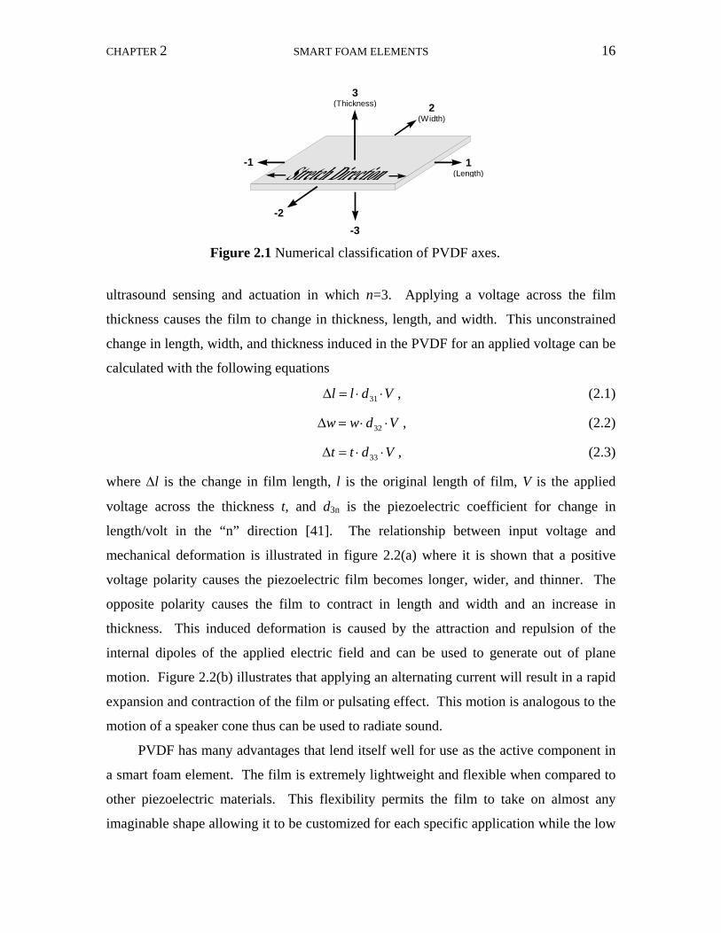
or electric field (for anisotropic materials). Figure 2.1 defines a standard numerical
classification for the film axes: 1 for length, 2 for width, and 3 for thickness. Two
subscripts are typically used when referring to the piezo-coefficients for charge dmn and
voltage gmn, but since we are using the PVDF as an actuator, we are most concerned with
the piezoelectric coefficient associated with change in length per applied voltage, or dmn.
The first subscript (m) refers to the electrical axis and the second subscript (n) refers to
the mechanical axis. In the case of piezoelectric film, the electrodes must be mounted to
transfer the voltage through the thickness of the film, and for this reason m is always 3 for
piezo-film. The mechanical axis subscript can be a 1, 2, or 3 depending on which axis is
of interest. Most sensing and actuation is done along the n=1 axis except for high
CHAPTER 2 SMART FOAM ELEMENTS 16
ultrasound sensing and actuation in which n=3. Applying a voltage across the film
thickness causes the film to change in thickness, length, and width. This unconstrained
change in length, width, and thickness induced in the PVDF for an applied voltage can be
calculated with the following equations
Vdll ⋅⋅=Δ 31 , (2.1)
Vdww ⋅⋅=Δ 32 , (2.2)
Vdtt ⋅⋅=Δ 33 , (2.3)
where Δl is the change in film length, l is the original length of film, V is the applied
voltage across the thickness t, and d3n is the piezoelectric coefficient for change in
length/volt in the “n” direction [41]. The relationship between input voltage and
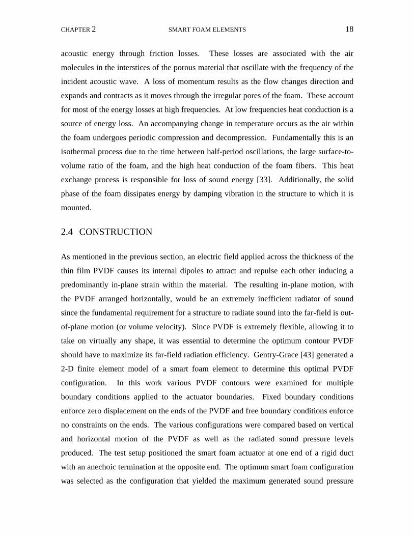
mechanical deformation is illustrated in figure 2.2(a) where it is shown that a positive
voltage polarity causes the piezoelectric film becomes longer, wider, and thinner. The
opposite polarity causes the film to contract in length and width and an increase in
thickness. This induced deformation is caused by the attraction and repulsion of the
internal dipoles of the applied electric field and can be used to generate out of plane
motion. Figure 2.2(b) illustrates that applying an alternating current will result in a rapid
expansion and contraction of the film or pulsating effect. This motion is analogous to the
motion of a speaker cone thus can be used to radiate sound.
PVDF has many advantages that lend itself well for use as the active component in
a smart foam element. The film is extremely lightweight and flexible when compared to
other piezoelectric materials. This flexibility permits the film to take on almost any
imaginable shape allowing it to be customized for each specific application while the low
-1
-2-3
2(Width)
1(Length)
3(Thickness)
Figure 2.1 Numerical classification of PVDF axes.
CHAPTER 2 SMART FOAM ELEMENTS 17
weight does not alter system characteristics by adding significant mass. A convenience
and cost advantage to using the film is that it can be bonded or glued using commercial
adhesives. A final advantage for using PVDF as the active element within smart foam is
the close match between the acoustic impedance of PVDF and that of air. The closer the
acoustic impedance of an actuator is to that of the medium on which it operates (air in
this case) the more efficient that source will radiate. The improved efficiency of the
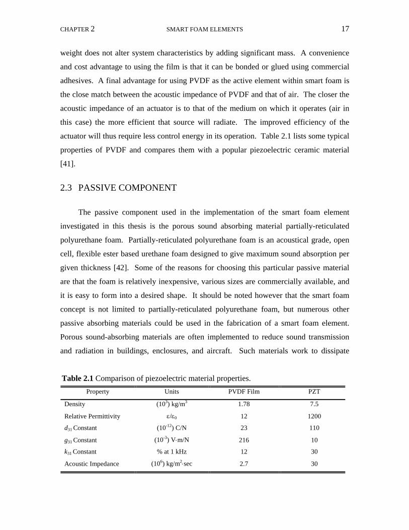
actuator will thus require less control energy in its operation. Table 2.1 lists some typical
properties of PVDF and compares them with a popular piezoelectric ceramic material
[41].
2.3 PASSIVE COMPONENT
The passive component used in the implementation of the smart foam element
investigated in this thesis is the porous sound absorbing material partially-reticulated
polyurethane foam. Partially-reticulated polyurethane foam is an acoustical grade, open
cell, flexible ester based urethane foam designed to give maximum sound absorption per
given thickness [42]. Some of the reasons for choosing this particular passive material
are that the foam is relatively inexpensive, various sizes are commercially available, and
it is easy to form into a desired shape. It should be noted however that the smart foam
concept is not limited to partially-reticulated polyurethane foam, but numerous other
passive absorbing materials could be used in the fabrication of a smart foam element.
Porous sound-absorbing materials are often implemented to reduce sound transmission
and radiation in buildings, enclosures, and aircraft. Such materials work to dissipate
Table 2.1 Comparison of piezoelectric material properties. Property Units PVDF Film PZT
Density (103) kg/m3 1.78 7.5
Relative Permittivity ε/ε0 12 1200
d31 Constant (10-12) C/N 23 110
g31 Constant (10-3) V⋅m/N 216 10
k31 Constant % at 1 kHz 12 30
Acoustic Impedance (106) kg/m2⋅sec 2.7 30
CHAPTER 2 SMART FOAM ELEMENTS 18
acoustic energy through friction losses. These losses are associated with the air
molecules in the interstices of the porous material that oscillate with the frequency of the
incident acoustic wave. A loss of momentum results as the flow changes direction and
expands and contracts as it moves through the irregular pores of the foam. These account
for most of the energy losses at high frequencies. At low frequencies heat conduction is a
source of energy loss. An accompanying change in temperature occurs as the air within
the foam undergoes periodic compression and decompression. Fundamentally this is an
isothermal process due to the time between half-period oscillations, the large surface-to-
volume ratio of the foam, and the high heat conduction of the foam fibers. This heat
exchange process is responsible for loss of sound energy [33]. Additionally, the solid
phase of the foam dissipates energy by damping vibration in the structure to which it is
mounted.
2.4 CONSTRUCTION As mentioned in the previous section, an electric field applied across the thickness of the
thin film PVDF causes its internal dipoles to attract and repulse each other inducing a
predominantly in-plane strain within the material. The resulting in-plane motion, with
the PVDF arranged horizontally, would be an extremely inefficient radiator of sound
since the fundamental requirement for a structure to radiate sound into the far-field is out-
of-plane motion (or volume velocity). Since PVDF is extremely flexible, allowing it to
take on virtually any shape, it was essential to determine the optimum contour PVDF
should have to maximize its far-field radiation efficiency. Gentry-Grace [43] generated a
2-D finite element model of a smart foam element to determine this optimal PVDF
configuration. In this work various PVDF contours were examined for multiple
boundary conditions applied to the actuator boundaries. Fixed boundary conditions
enforce zero displacement on the ends of the PVDF and free boundary conditions enforce
no constraints on the ends. The various configurations were compared based on vertical
and horizontal motion of the PVDF as well as the radiated sound pressure levels
produced. The test setup positioned the smart foam actuator at one end of a rigid duct
with an anechoic termination at the opposite end. The optimum smart foam configuration
was selected as the configuration that yielded the maximum generated sound pressure
CHAPTER 2 SMART FOAM ELEMENTS 19
levels between 100 Hz and 1000 Hz excited at 300 Vrms. This work demonstrated that
more vertical displacement could be achieved by increasing the radius of the half-
cylinder. A larger radius requires a longer piece of PVDF and thus yields a greater
change in length (Δl) for an applied voltage (V) per equation (2.1). C. Liang et al. [44]
also conducted analytical studies concerning curved PVDF which showed that the
acoustic intensity generated by an actuator in the low-frequency region is directly
proportional to the radius of the PVDF.
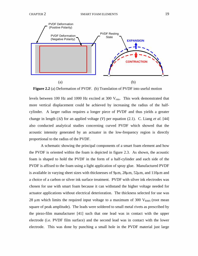
A schematic showing the principal components of a smart foam element and how
the PVDF is oriented within the foam is depicted in figure 2.3. As shown, the acoustic
foam is shaped to hold the PVDF in the form of a half-cylinder and each side of the
PVDF is affixed to the foam using a light application of spray glue. Manufactured PVDF
is available in varying sheet sizes with thicknesses of 9μm, 28μm, 52μm, and 110μm and
a choice of a carbon or silver ink surface treatment. PVDF with silver ink electrodes was
chosen for use with smart foam because it can withstand the higher voltage needed for
actuator applications without electrical deterioration. The thickness selected for use was
28 μm which limits the required input voltage to a maximum of 300 VRMS (root mean
square of peak amplitude). The leads were soldered to small metal rivets as prescribed by
the piezo-film manufacturer [41] such that one lead was in contact with the upper
electrode (i.e. PVDF film surface) and the second lead was in contact with the lower
electrode. This was done by punching a small hole in the PVDF material just large
PVDF RestingState
PVDF Deformation (Positive Polarity)
PVDF Deformation (Negative Polarity) EXPANSION
CONTRACTION
(a) (b)
Figure 2.2 (a) Deformation of PVDF. (b) Translation of PVDF into useful motion
CHAPTER 2 SMART FOAM ELEMENTS 20
enough for the rivet to pass through. On the back side of the film the silver electrode
material was removed using acetone and a Q-tip, a process called etching. This
procedure assured that the rivet only contacted a single side of the PVDF once it was
crimped in place. One rivet, with the electrical lead soldered in place, was inserted
through the film from one direction and the other is inserted in the opposite direction.
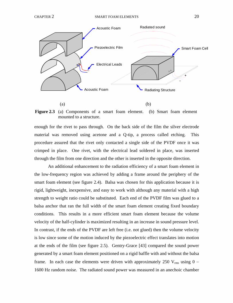
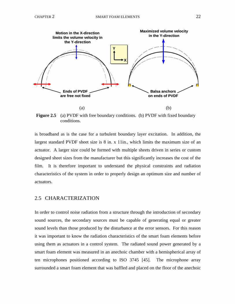
An additional enhancement to the radiation efficiency of a smart foam element in
the low-frequency region was achieved by adding a frame around the periphery of the
smart foam element (see figure 2.4). Balsa was chosen for this application because it is
rigid, lightweight, inexpensive, and easy to work with although any material with a high
strength to weight ratio could be substituted. Each end of the PVDF film was glued to a
balsa anchor that ran the full width of the smart foam element creating fixed boundary
conditions. This results in a more efficient smart foam element because the volume
velocity of the half-cylinder is maximized resulting in an increase in sound pressure level.
In contrast, if the ends of the PVDF are left free (i.e. not glued) then the volume velocity
is low since some of the motion induced by the piezoelectric effect translates into motion
at the ends of the film (see figure 2.5). Gentry-Grace [43] compared the sound power
generated by a smart foam element positioned on a rigid baffle with and without the balsa
frame. In each case the elements were driven with approximately 250 Vrms using 0 −
1600 Hz random noise. The radiated sound power was measured in an anechoic chamber
(a) (b)
Figure 2.3 (a) Components of a smart foam element. (b) Smart foam element mounted to a structure.
+
Acoustic Foam
Piezoelectric Film
Acoustic Foam
Radiated sound
Radiating Structure
Smart Foam Cell
Electrical Leads
CHAPTER 2 SMART FOAM ELEMENTS 21
with a hemispherical array of ten microphones positioned according to ISO 3745 [45].
The addition of the balsa frame resulted in an increase of 10 dB of radiated sound power
in the 200 − 650 Hz range.
It has been determined that PVDF in the form of a half-cylinder with a
maximized radius is the most efficient configuration for radiation efficiency because
large actuator displacements result. Given this fact alone it would be concluded that the
smart foam element should be as large as possible in order to maximize the achievable
impact from a single actuator element. There are other factors specific to each
application to consider that influence the size and shape of a smart foam element. A
vibrating structure will have varying radiation characteristics (modes) resulting from both
the physical properties of the structure and the nature of the excitation. If it is desired to
control the radiation from the vibrating structure, it is necessary to have an actuator
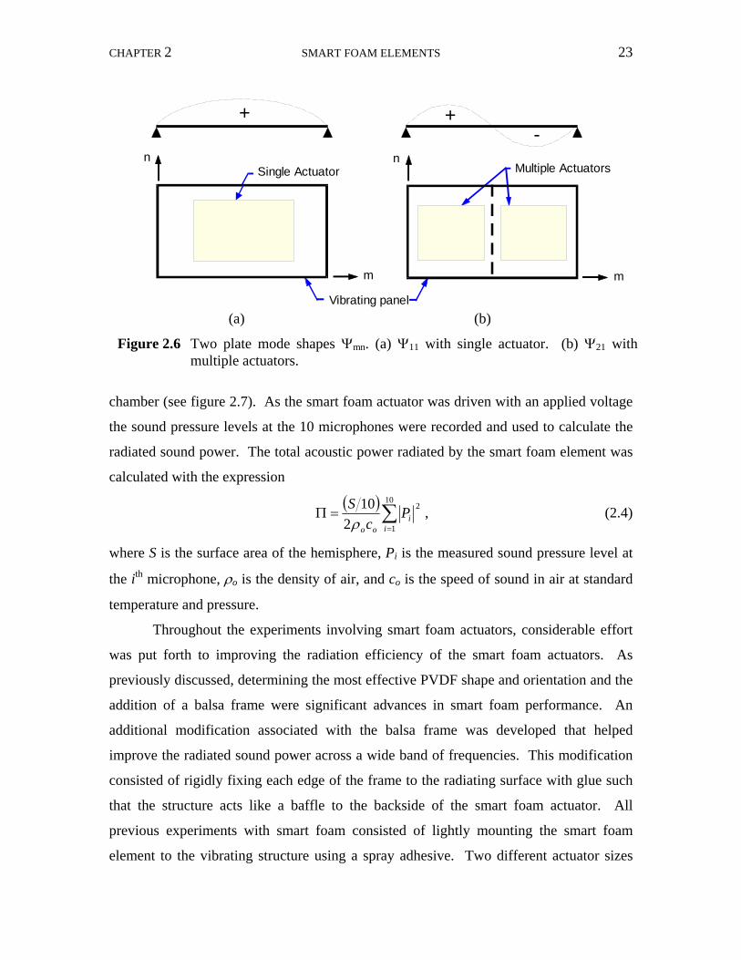
configuration with control authority over the radiating modes. As an example, a panel
vibrating in its first structural mode (1,1) acts like a monopole and could easily be
controlled with a single active source centered on the panel. A panel vibrating in a
second order mode (2,1) acts like a dipole and would require two active sources for
effective control (see figure 2.6). Dual actuators as in figure 2.6(b) are optimally
configured to control the (2,1) mode but, can also control the (1,1) mode by having each
actuator driven together in phase. Radiating structures typically consists of contributions
from many modes shapes that are excited by the disturbance, especially if the disturbance
Rigid Frame (Balsa)Balsa anchors for fixed
boundary conditions
PVDF FilmAcoustic Foam
Figure 2.4 Smart foam element.
CHAPTER 2 SMART FOAM ELEMENTS 22
is broadband as is the case for a turbulent boundary layer excitation. In addition, the
largest standard PVDF sheet size is 8 in. x 11in., which limits the maximum size of an
actuator. A larger size could be formed with multiple sheets driven in series or custom
designed sheet sizes from the manufacturer but this significantly increases the cost of the
film. It is therefore important to understand the physical constraints and radiation
characteristics of the system in order to properly design an optimum size and number of
actuators.
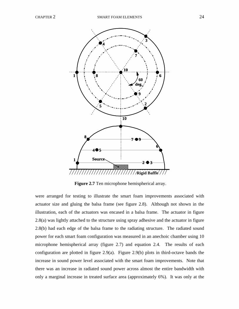
2.5 CHARACTERIZATION In order to control noise radiation from a structure through the introduction of secondary
sound sources, the secondary sources must be capable of generating equal or greater
sound levels than those produced by the disturbance at the error sensors. For this reason
it was important to know the radiation characteristics of the smart foam elements before
using them as actuators in a control system. The radiated sound power generated by a
smart foam element was measured in an anechoic chamber with a hemispherical array of
ten microphones positioned according to ISO 3745 [45]. The microphone array
surrounded a smart foam element that was baffled and placed on the floor of the anechoic
Balsa anchors Balsa anchors on ends of PVDFon ends of PVDF
Maximized volume velocity Maximized volume velocity in the Yin the Y--directiondirection
XX
YY
XX
YY
Ends of PVDF Ends of PVDF are free not fixedare free not fixed
Motion in the XMotion in the X--direction direction limits the volume velocity in limits the volume velocity in
the Ythe Y--directiondirection
(a) (b)
Figure 2.5 (a) PVDF with free boundary conditions. (b) PVDF with fixed boundary conditions.
CHAPTER 2 SMART FOAM ELEMENTS 23
chamber (see figure 2.7). As the smart foam actuator was driven with an applied voltage
the sound pressure levels at the 10 microphones were recorded and used to calculate the
radiated sound power. The total acoustic power radiated by the smart foam element was
calculated with the expression
( )∑=
=Π10
1
2
210
ii
oo
Pc
Sρ
, (2.4)
where S is the surface area of the hemisphere, Pi is the measured sound pressure level at
the ith microphone, ρo is the density of air, and co is the speed of sound in air at standard
temperature and pressure.
Throughout the experiments involving smart foam actuators, considerable effort
was put forth to improving the radiation efficiency of the smart foam actuators. As
previously discussed, determining the most effective PVDF shape and orientation and the
addition of a balsa frame were significant advances in smart foam performance. An
additional modification associated with the balsa frame was developed that helped
improve the radiated sound power across a wide band of frequencies. This modification
consisted of rigidly fixing each edge of the frame to the radiating surface with glue such
that the structure acts like a baffle to the backside of the smart foam actuator. All
previous experiments with smart foam consisted of lightly mounting the smart foam
element to the vibrating structure using a spray adhesive. Two different actuator sizes
(a) (b)
Figure 2.6 Two plate mode shapes Ψmn. (a) Ψ11 with single actuator. (b) Ψ21 with multiple actuators.
-+ +
m
Vibrating panel
Multiple Actuatorsn n
Single Actuator
m
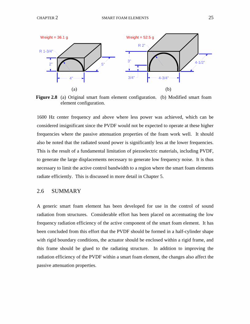
CHAPTER 2 SMART FOAM ELEMENTS 24
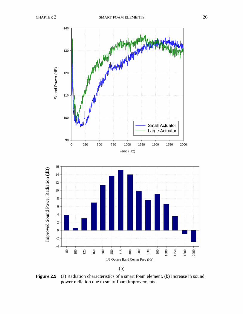
were arranged for testing to illustrate the smart foam improvements associated with
actuator size and gluing the balsa frame (see figure 2.8). Although not shown in the
illustration, each of the actuators was encased in a balsa frame. The actuator in figure
2.8(a) was lightly attached to the structure using spray adhesive and the actuator in figure
2.8(b) had each edge of the balsa frame to the radiating structure. The radiated sound
power for each smart foam configuration was measured in an anechoic chamber using 10
microphone hemispherical array (figure 2.7) and equation 2.4. The results of each
configuration are plotted in figure 2.9(a). Figure 2.9(b) plots in third-octave bands the
increase in sound power level associated with the smart foam improvements. Note that
there was an increase in radiated sound power across almost the entire bandwidth with
only a marginal increase in treated surface area (approximately 6%). It was only at the
1
2
34
5
6
7
8
9
10
60deg.
1 2 3
4 56
78 9
10
Rigid Baffle
Source
1
2
34
5
6
7
8
9
10
60deg.
1 2 3
4 56
78 9
10
Rigid Baffle
Source
Figure 2.7 Ten microphone hemispherical array.
CHAPTER 2 SMART FOAM ELEMENTS 25
1600 Hz center frequency and above where less power was achieved, which can be
considered insignificant since the PVDF would not be expected to operate at these higher
frequencies where the passive attenuation properties of the foam work well. It should
also be noted that the radiated sound power is significantly less at the lower frequencies.
This is the result of a fundamental limitation of piezoelectric materials, including PVDF,
to generate the large displacements necessary to generate low frequency noise. It is thus
necessary to limit the active control bandwidth to a region where the smart foam elements
radiate efficiently. This is discussed in more detail in Chapter 5.
2.6 SUMMARY A generic smart foam element has been developed for use in the control of sound
radiation from structures. Considerable effort has been placed on accentuating the low
frequency radiation efficiency of the active component of the smart foam element. It has
been concluded from this effort that the PVDF should be formed in a half-cylinder shape
with rigid boundary conditions, the actuator should be enclosed within a rigid frame, and
this frame should be glued to the radiating structure. In addition to improving the
radiation efficiency of the PVDF within a smart foam element, the changes also affect the
passive attenuation properties.
(a) (b)
Figure 2.8 (a) Original smart foam element configuration. (b) Modified smart foam element configuration.
2”
4”
5”
R 1-3/4”
3”
R 2”
3/4” 4-3/4”
4-1/2”
Weight = 36.1 g Weight = 52.5 g
CHAPTER 2 SMART FOAM ELEMENTS 26
(a)
(b)
Figure 2.9 (a) Radiation characteristics of a smart foam element. (b) Increase in sound power radiation due to smart foam improvements.
1/3 Octave Band Center Freq (Hz)
80 100
125
160
200
250
315
400
500
630
800
1000
1250
1600
2000
Impr
oved
Sou
nd P
ower
Rad
iatio
n (d
B re
10-1
2 Wat
ts)
-4
-2
0
2
4
6
8
10
12
14
16
Impr
oved
Sou
nd P
ower
Rad
iatio
n (d
B)
Freq (Hz)
0 250 500 750 1000 1250 1500 1750 2000
Sou
nd P
ower
(dB
re 1
0-12 W
atts
)
90
100
110
120
130
140
Small ActuatorLarge Actuator
Soun
d Po
wer
(dB)
27
Chapter 3 Control Methodology 3.1 INTRODUCTION Paul Lueg first introduced controlling unwanted noise by the introduction of additional
sound when he filed for a US patent in 1934 [46]. The system Lueg proposed was
designed to control plane wave sound in a duct and consisted of an upstream microphone
for detecting the propagating sound waves and a downstream loudspeaker used as a
secondary noise source. The two components were linked with an electronic control
system that was responsible for adding an appropriate delay and amplification to the
detected signal such that the emitted signal at the speaker was an inverted duplicate of the
disturbance. Lueg’s system was practically the same methodology and contained the
same components as systems implemented in many of today’s commercial active noise
control systems. Although this concept was developed in 1934, the problem of
implementing control systems to solve real problems was limited due to the inability to
process the required data efficiently and accurately. Recently, with the advent of
inexpensive digital signal processors (DSP), these feedforward control techniques are
now practical solutions to numerous control problems. Not only are they implemented to
control plane wave sound propagation in ducts, as Lueg illustrated in his patent, but also
multi-channel systems with less predictable disturbance characteristics, such as those
induced by a turbulent boundary layer.
The following sections will give a brief introduction into the development of a
filtered-x LMS control algorithm [47]. This discussion will then expand to include the
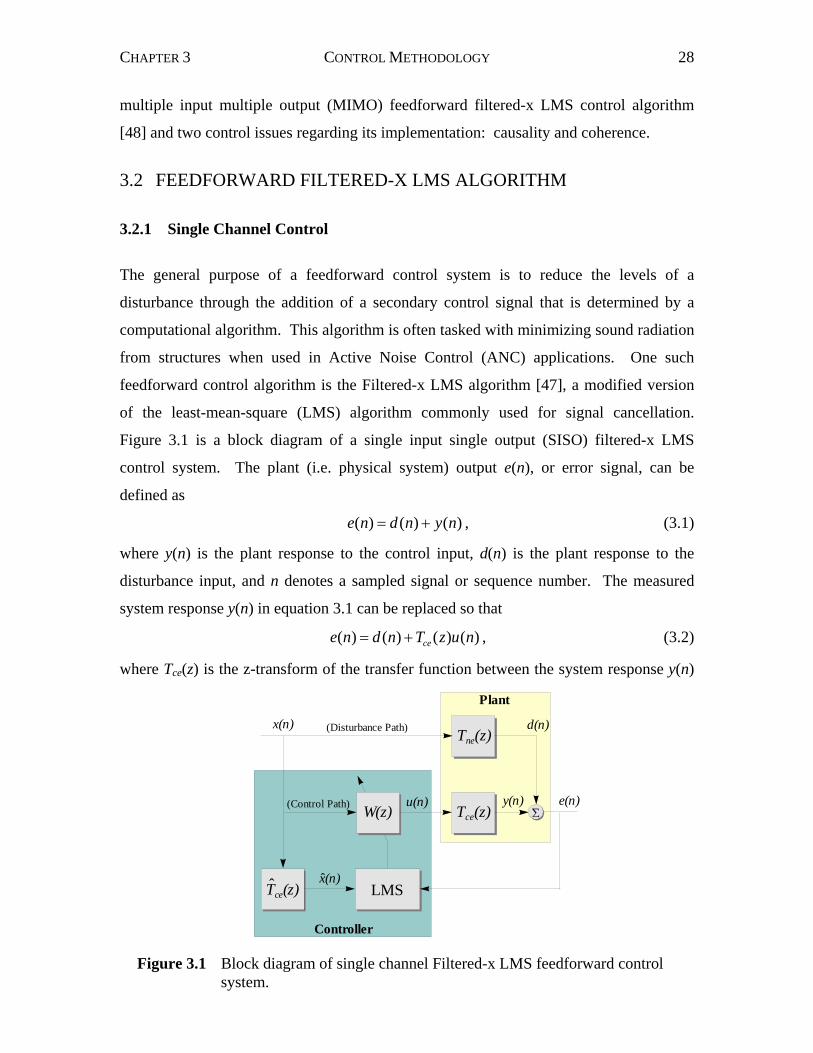
CHAPTER 3 CONTROL METHODOLOGY 28
multiple input multiple output (MIMO) feedforward filtered-x LMS control algorithm
[48] and two control issues regarding its implementation: causality and coherence.
3.2 FEEDFORWARD FILTERED-X LMS ALGORITHM 3.2.1 Single Channel Control
The general purpose of a feedforward control system is to reduce the levels of a
disturbance through the addition of a secondary control signal that is determined by a
computational algorithm. This algorithm is often tasked with minimizing sound radiation
from structures when used in Active Noise Control (ANC) applications. One such
feedforward control algorithm is the Filtered-x LMS algorithm [47], a modified version
of the least-mean-square (LMS) algorithm commonly used for signal cancellation.
Figure 3.1 is a block diagram of a single input single output (SISO) filtered-x LMS
control system. The plant (i.e. physical system) output e(n), or error signal, can be
defined as
)()()( nyndne += , (3.1)
where y(n) is the plant response to the control input, d(n) is the plant response to the
disturbance input, and n denotes a sampled signal or sequence number. The measured
system response y(n) in equation 3.1 can be replaced so that
)()()()( nuzTndne ce+= , (3.2)
where Tce(z) is the z-transform of the transfer function between the system response y(n)
Controller
Plant
Tne(z)
W(z)
LMST̂ce(z)
d(n)
e(n)
x(n)
x̂(n)
u(n) y(n)ΣTce(z)
(Disturbance Path)
(Control Path)
Figure 3.1 Block diagram of single channel Filtered-x LMS feedforward control system.
CHAPTER 3 CONTROL METHODOLOGY 29
and the control sequence u(n).
The control sequence u(n) is the output signal from the controller and is obtained
from the adaptive FIR (Finite Impulse Response) filter represented as W(z). The adaptive
FIR filter is a fundamental component used in the implementation of many control
algorithms and is characterized by having zero impulse response after a set number of
samples. A FIR filter generates an output to a digital system that is the weighted sum of
previous input values, so that
)()()(1
0
inxnWnyI
ii −=∑
−
=
, (3.3)
where )(nWi is the ith filter coefficient and I is the filter order. A block diagram
representation of this difference equation is shown in figure 3. where 1−z denotes a unit
delay operator. This operator, when performed on a sequence, introduces a delay by one
sample such that )1()(1 −=− nxnxz . The adaptive FIR filter, W(z), can thus be
represented as an operator such that
)1(1
22
110)( −−
−−− ++++= I
L zWzWzWWzW L , (3.4)
∑−
=
−=1
0
I
i
ii zW , (3.5)
and consequently the control sequence can be defined as
)()()( nxzWnu = . (3.6)
Substituting equation 3.6 into equation 3.2, the plant output, or error becomes
)()()()()( nxzWzTndne ce+= . (3.7)
An error criterion, or cost function, must now be defined such that the plant input
signal u(n) can be adjusted to minimize the plant response e(n). The most commonly
used cost function for active noise control is defined as
)]([E)( 2 neWC i = , (3.8)
where E[e2(n)] is the expected value of the mean-square error signal and is a quadratic
function of the filter coefficients. In the frequency domain, he quadratic cost function, or
performance surface, can be plotting for visualization as a function of the real and
imaginary components of the plant input u(n) and has a unique global minima. This
performance surface is a bowl-shaped error function where the elliptical contour lines
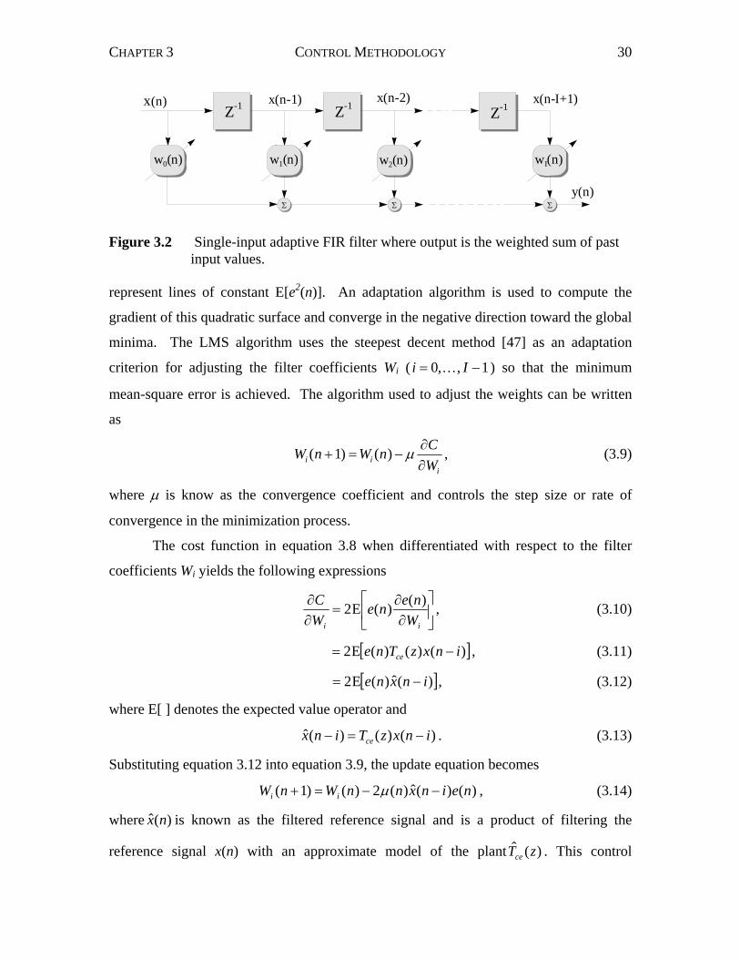
CHAPTER 3 CONTROL METHODOLOGY 30
represent lines of constant E[e2(n)]. An adaptation algorithm is used to compute the
gradient of this quadratic surface and converge in the negative direction toward the global
minima. The LMS algorithm uses the steepest decent method [47] as an adaptation
criterion for adjusting the filter coefficients Wi ( 1,,0 −= Ii K ) so that the minimum
mean-square error is achieved. The algorithm used to adjust the weights can be written
as
i
ii WCnWnW
∂∂
−=+ μ)()1( , (3.9)
where μ is know as the convergence coefficient and controls the step size or rate of
convergence in the minimization process.
The cost function in equation 3.8 when differentiated with respect to the filter
coefficients Wi yields the following expressions
⎥⎦
⎤⎢⎣
⎡∂∂
=∂∂
ii Wnene
WC )()(E2 , (3.10)
[ ])()()(E2 inxzTne ce −= , (3.11)
[ ])(ˆ)(E2 inxne −= , (3.12)
where E[ ] denotes the expected value operator and
)()()(ˆ inxzTinx ce −=− . (3.13)
Substituting equation 3.12 into equation 3.9, the update equation becomes
)()(ˆ)(2)()1( neinxnnWnW ii −−=+ μ , (3.14)
where )(ˆ nx is known as the filtered reference signal and is a product of filtering the
reference signal x(n) with an approximate model of the plant )(ˆ zTce . This control
Z-1 Z-1 Z-1x(n) x(n-1)
y(n)
w0(n)
Σ Σ Σ
x(n-2) x(n-I+1)
w1(n) w2(n) wI(n)
Figure 3.2 Single-input adaptive FIR filter where output is the weighted sum of past input values.
CHAPTER 3 CONTROL METHODOLOGY 31
algorithm is known as the filtered-x LMS algorithm. The plant model )(ˆ zTce is built using
a FIR filter in which the LMS algorithm adapts the filter coefficients while driving the
actuator and measuring the response at the error sensor e(n). This process is performed
off-line and is know as the system identification.
The convergence coefficient μ controls the step size the LMS algorithm takes as it
iterates to the global minimum of the quadratic cost function. As the convergence
coefficient μ increases, the time for convergence decreases. Large μ values can,
however, cause the algorithm to become unstable where the control inputs increase
without bounds. Widrow et al. [47] states that in general, the stability of the algorithm
can be calculated using the input autocorrelation matrix R such that
][
10RTrace
<< μ , (3.15)
where
∑=
=I
ii nxRTrace
0
2 )(][ . (3.16)
A large value of μ results in quicker convergence time but a large coefficient may cause
the algorithm to step over the minimum value during iteration. In order to assure quick
convergence on the surface minima, the convergence parameter μ should be set high for
initial convergence and then reduced to assure that the minima is obtained.
There are several general properties of the filtered-x LMS algorithm that make it
an advantages choice for use in noise control applications [12]:
1. Changes in the disturbance signal are rapidly tracked because the algorithm
can converge on a time scale comparable with the delay in the error path.
2. The algorithm is robust to errors in the estimation of the error path used to
generate the filtered reference signal.
3. The algorithm is easy to implement, only differing from the LMS algorithm in
that it requires the generation of the filtered reference signal.
The algorithm does have limitations, however, that exist from poor coherence
between reference and disturbance signal, inaccurate model of the plant, low control
CHAPTER 3 CONTROL METHODOLOGY 32
filter order, and low sample rate. Each of these limitations, with the exception of
poor coherence, is a function of the processing speed of the DSP.
3.2.2 Multiple-Channel Control
It may not always be possible to obtain global noise control with the introduction of a
single error sensor and secondary source. Often the primary disturbance or the radiated
sound field is such that it requires the introduction of multiple sources and error sensors
to achieve global control or control over a large volume. The filtered-x LMS algorithm
has been developed for use with multiple secondary control sources and error sensors
[48]. The modified update equation for each control filter coefficient with L sensors and
M actuators is
∑=
−−=+L
lllmmimi neinxnWnW
1
)()(ˆ2)()1( μ , (3.17)
where )(ˆ nxlm is the reference signal filtered with a model of the system path from the mth
actuator and the lth error sensor at sample n. Note that equation 3.17 is equivalent to the
SISO system of equation 3.14 when L = M = 1. In addition, the level of control that can
be obtained by a control system also depends on the quality of the reference signal used
to capture the dynamics of the disturbance. For a spatially incoherent disturbance, as
provided by a turbulent boundary layer, multiple references (K) may be required to
achieve adequate control levels. The multiple-channel controller now contains MK finite
impulse response filters each updated by the control algorithm. Section 3.3.2 discusses
multiple coherence and presents a control example that helps to quantify the benefits of
using multiple reference signals.
3.3 PRACTICAL IMPLEMENTATION OF CONTROL ALGORITHM All experiments conducted in this work utilized the multi-channel version of the filtered-
x LMS algorithm. The control code was written in Assembly and C programming
languages for a Spectrum Quad TMS320C40 digital signal processor (DSP). The DSP
processes data using 4 parallel processors and therefore the system runs at peak
efficiency when the computation can be divided easily into multiples of 4. Flexibility has
CHAPTER 3 CONTROL METHODOLOGY 33
been incorporated into the control code so that numerous control scenarios can be
examined using the same controller. Control performance for a particular set of control
parameters may have been compromised, however, to account for the built-in flexibility.
To take full advantage of the computing capabilities of the DSP, the control code could
have been customized for each set of control parameters, but this would have resulted in
countless configurations and was not practical for this phase of the project.
Virginia Tech has developed a LabVIEW® interface program for use with the
multi-channel controller that allows the user to easily choose a desired set of control
parameters. The following is a methodology and procedure for using the multi-channel
filtered-x LMS control algorithm that Virginia Tech has implemented. Details about the
flexibility built into the controller will also be included in the procedure.
1. Select the number of reference sensors (4), error sensors (8), and actuators (8)
to be used in the experiments. The value in parentheses is the maximum value
allowed by the program.
2. Select the sampling frequency, system ID coefficients, and control path
coefficients. The system ID coefficients are the number of FIR filter
coefficients that are used to build the model of the plant )(ˆ zTce , through which
the reference signal x(n) is filtered. The control path coefficients are the
number of coefficients present in the adaptive FIR filter W(z) that are updated
by the LMS algorithm to generate the secondary control signal.
3. Set the system coupling. A fully coupled system will model the control paths
from an actuator to each of the error sensors, whereas an uncoupled system
will model the control path from an actuator to a single error sensor.
Typically the control results are best when the system is fully coupled.
4. The controller builds the plant models )(ˆ zTce , or a matrix of transfer functions,
by sequentially driving each actuator and measuring the response at all of the
error microphones (e.g. )(ˆ zTce will be a 4 x 4 matrix if a system has 4
actuators and 4 error sensors).
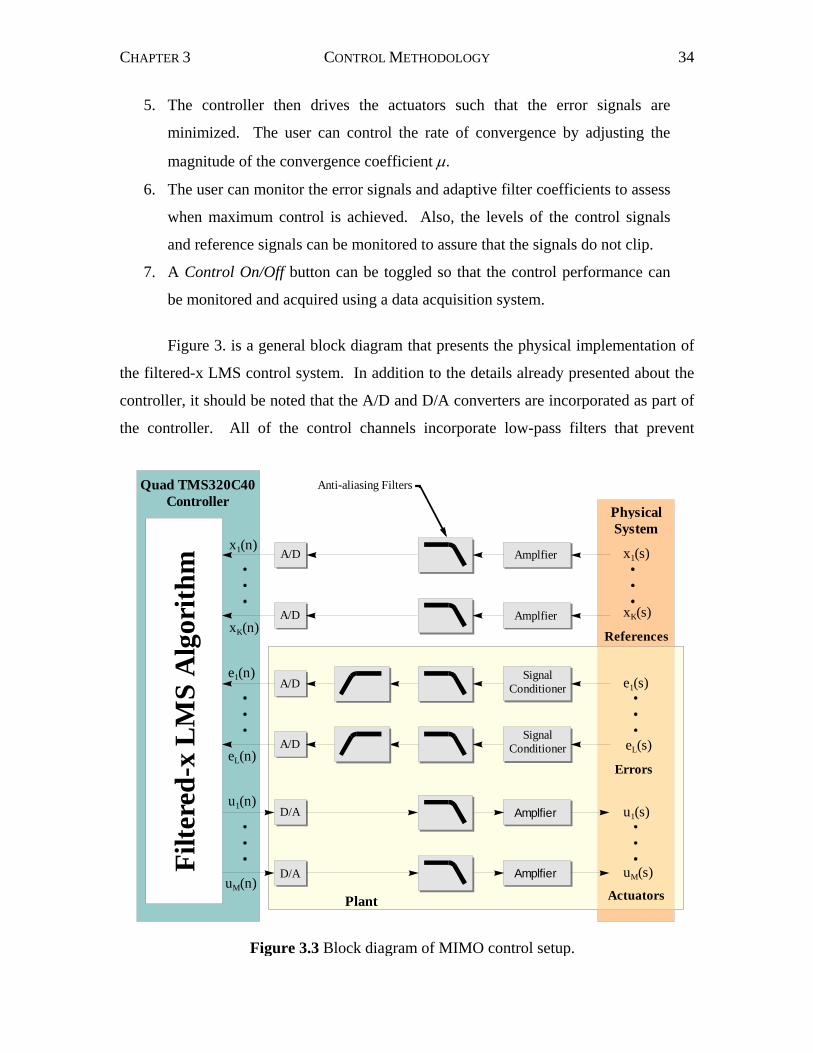
CHAPTER 3 CONTROL METHODOLOGY 34
5. The controller then drives the actuators such that the error signals are
minimized. The user can control the rate of convergence by adjusting the
magnitude of the convergence coefficient μ.
6. The user can monitor the error signals and adaptive filter coefficients to assess
when maximum control is achieved. Also, the levels of the control signals
and reference signals can be monitored to assure that the signals do not clip.
7. A Control On/Off button can be toggled so that the control performance can
be monitored and acquired using a data acquisition system.
Figure 3. is a general block diagram that presents the physical implementation of
the filtered-x LMS control system. In addition to the details already presented about the
controller, it should be noted that the A/D and D/A converters are incorporated as part of
the controller. All of the control channels incorporate low-pass filters that prevent
Filte
red-
x L
MS
Alg
orith
m
Quad TMS320C40Controller
A/D
A/D
A/D
D/A
D/A
Amplfier
Amplfier
Amplfier
Signal Conditioner
Signal Conditioner
A/D Amplfier x1(s)
xK(s)
e1(s)
u1(s)
uM(s)
PhysicalSystem
x1(n)
xK(n)
e1(n)
eL(n)
u1(n)
uM(n)
References
eL(s)
Errors
ActuatorsPlant
Anti-aliasing Filters
Figure 3.3 Block diagram of MIMO control setup.
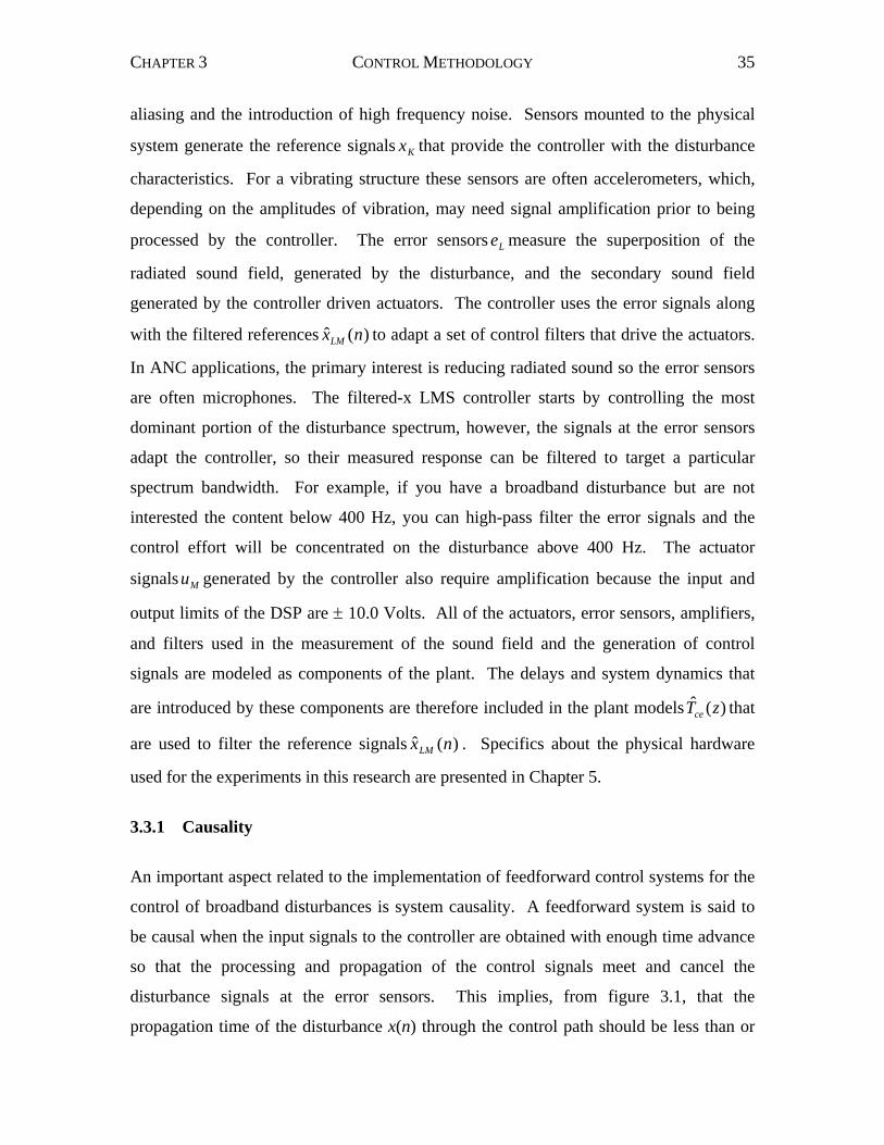
CHAPTER 3 CONTROL METHODOLOGY 35
aliasing and the introduction of high frequency noise. Sensors mounted to the physical
system generate the reference signals Kx that provide the controller with the disturbance
characteristics. For a vibrating structure these sensors are often accelerometers, which,
depending on the amplitudes of vibration, may need signal amplification prior to being
processed by the controller. The error sensors Le measure the superposition of the
radiated sound field, generated by the disturbance, and the secondary sound field
generated by the controller driven actuators. The controller uses the error signals along
with the filtered references )(ˆ nxLM to adapt a set of control filters that drive the actuators.
In ANC applications, the primary interest is reducing radiated sound so the error sensors
are often microphones. The filtered-x LMS controller starts by controlling the most
dominant portion of the disturbance spectrum, however, the signals at the error sensors
adapt the controller, so their measured response can be filtered to target a particular
spectrum bandwidth. For example, if you have a broadband disturbance but are not
interested the content below 400 Hz, you can high-pass filter the error signals and the
control effort will be concentrated on the disturbance above 400 Hz. The actuator
signals Mu generated by the controller also require amplification because the input and
output limits of the DSP are ± 10.0 Volts. All of the actuators, error sensors, amplifiers,
and filters used in the measurement of the sound field and the generation of control
signals are modeled as components of the plant. The delays and system dynamics that
are introduced by these components are therefore included in the plant models )(ˆ zTce that
are used to filter the reference signals )(ˆ nxLM . Specifics about the physical hardware
used for the experiments in this research are presented in Chapter 5. 3.3.1 Causality
An important aspect related to the implementation of feedforward control systems for the
control of broadband disturbances is system causality. A feedforward system is said to
be causal when the input signals to the controller are obtained with enough time advance
so that the processing and propagation of the control signals meet and cancel the
disturbance signals at the error sensors. This implies, from figure 3.1, that the
propagation time of the disturbance x(n) through the control path should be less than or
CHAPTER 3 CONTROL METHODOLOGY 36
equal to the propagation time through the disturbance path. Causality is only an issue
when the disturbance is broadband since a sinusoidal excitation is deterministic in nature
and its future values can always be predicted under steady-state conditions.
The level of performance that can be achieved with a feedforward control system
diminishes when causality is not satisfied. Burdisso et al. [49] proposed an analytical
approach to predicting the control performance of non-causal feedforward control
systems with broadband inputs. This work demonstrated that some level of reduction in
the error signal mean-square value is always achievable for any non-causal control
system.
Control path delays can result from the use of anti-aliasing filters, the process of
sampling, and the physical characteristics of the plant. These delays can be compensated
for in systems with compact noise sources because the reference can be placed upstream
close to the source, however, this is not as easy for distributed disturbances such as
turbulent boundary layer noise. The analysis by Burdisso et al. [49] did show that the
deterioration in the control performance due to the delays in the control path could be
partially compensated by increasing the order of the control filter W(z).
3.3.2 Multiple Coherence
The maximum level of control that can be achieved by a feedforward filtered-x LMS is
determined by the coherence between the reference signal and the disturbance signal.
The ordinary coherence function is defined as
)()(
)()(
22
fSfSfS
fddxx
xdxd =γ , 1)(0 2 ≤≤ fxdγ , (3.18)
and is a measure of the extent to which an output signal d(n) may be predicted from an
input signal x(n) by an optimum linear least-squares relationship [47]. The notation used
was selected to be consistent with figure 3.1, where the subscript x refers to the reference
signal and d the signal at the error sensor due to the primary disturbance plus any
measurement noise. The cross-spectral density function is represented by )( fSxd , where
the input and output autospectral density functions are represented by )( fSxx and )( fSdd
CHAPTER 3 CONTROL METHODOLOGY 37
respectively. The coherent output spectrum )( fSvv can be defined in terms of the output
autospectral density function )( fSdd such that
)()()( 2 fSffS ddxdvv γ= , (3.19)
and the associated noise output spectrum is given by
)()](1[)( 2 fSffS ddxdnn γ−= . (3.20)
Note that when )(2 fxdγ is equal to 1 the output noise spectrum )( fSnn is 0, and the
coherent output spectrum )( fSvv is equivalent to the output autospectral density function
)( fSdd [47]. In a linear feedforward control system, )( fSvv represents the controllable
portion of the error signal and )( fSnn the uncontrollable portion, therefore, these
quantities can be used to estimate the performance of an active control system. For
example, at a particular frequency a coherence value of )(2 fxdγ = 0.99 will yield a
maximum of 20 dB attenuation and )(2 fxdγ = 0.9 produces 10 dB attenuation.
It has been shown that the potential attenuation of a single-channel active control
system depends on the level of coherence between the error and reference signals. A
similar correlation has been developed, in which a multiple coherence function [12] is
used as a performance estimation tool for multi-channel active control systems. In a
multi-channel system, a single error signal has information about the disturbance
characteristics due to all of the reference signals and not just a single reference, as is the
case for the ordinary coherence function. The multiple coherence function is defined as
)(
)()()()(1
2
fSffff
dd
xdxxHxd
xdsSs −
=γ , 1)(0 2 ≤≤ fxdγ , (3.21)
where )( fxds is a vector of cross-spectra between each reference sensor and the signal at
a single-error sensor. The cross-spectra between each of the reference sensors is
represented by the matrix )( fxxS and )( fSdd is the power spectral density of the signal at
the error sensor due to the primary field and measurement noise. A Hermitian transpose
is performed on the vector )( fxds , denoted by the superscript H, and is defined as the
complex conjugate of the transpose
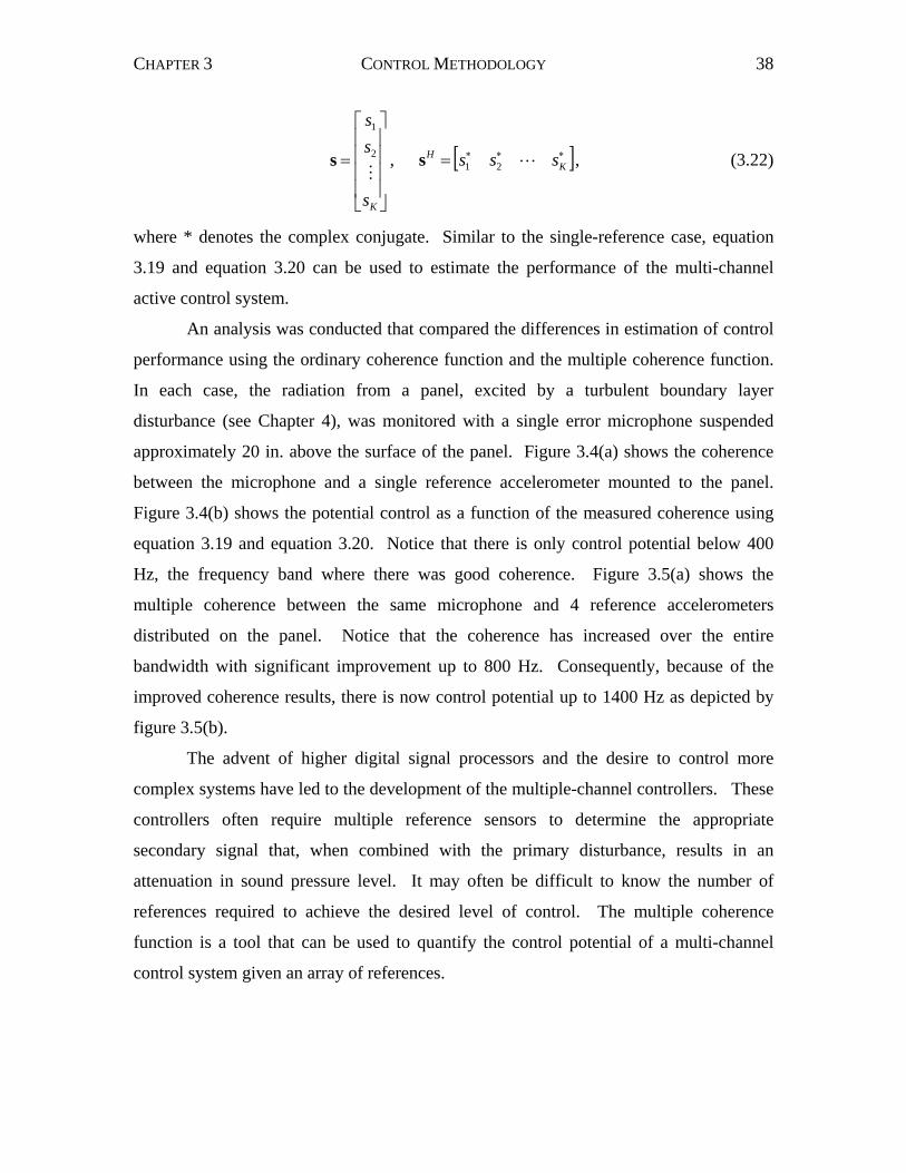
CHAPTER 3 CONTROL METHODOLOGY 38
⎥⎥⎥⎥
⎦
⎤
⎢⎢⎢⎢
⎣
⎡
=
Ks
ss
M2
1
s , [ ]∗∗∗= KH sss L21s , (3.22)
where * denotes the complex conjugate. Similar to the single-reference case, equation
3.19 and equation 3.20 can be used to estimate the performance of the multi-channel
active control system.
An analysis was conducted that compared the differences in estimation of control
performance using the ordinary coherence function and the multiple coherence function.
In each case, the radiation from a panel, excited by a turbulent boundary layer
disturbance (see Chapter 4), was monitored with a single error microphone suspended
approximately 20 in. above the surface of the panel. Figure 3.4(a) shows the coherence
between the microphone and a single reference accelerometer mounted to the panel.
Figure 3.4(b) shows the potential control as a function of the measured coherence using
equation 3.19 and equation 3.20. Notice that there is only control potential below 400
Hz, the frequency band where there was good coherence. Figure 3.5(a) shows the
multiple coherence between the same microphone and 4 reference accelerometers
distributed on the panel. Notice that the coherence has increased over the entire
bandwidth with significant improvement up to 800 Hz. Consequently, because of the
improved coherence results, there is now control potential up to 1400 Hz as depicted by
figure 3.5(b).
The advent of higher digital signal processors and the desire to control more
complex systems have led to the development of the multiple-channel controllers. These
controllers often require multiple reference sensors to determine the appropriate
secondary signal that, when combined with the primary disturbance, results in an
attenuation in sound pressure level. It may often be difficult to know the number of
references required to achieve the desired level of control. The multiple coherence
function is a tool that can be used to quantify the control potential of a multi-channel
control system given an array of references.
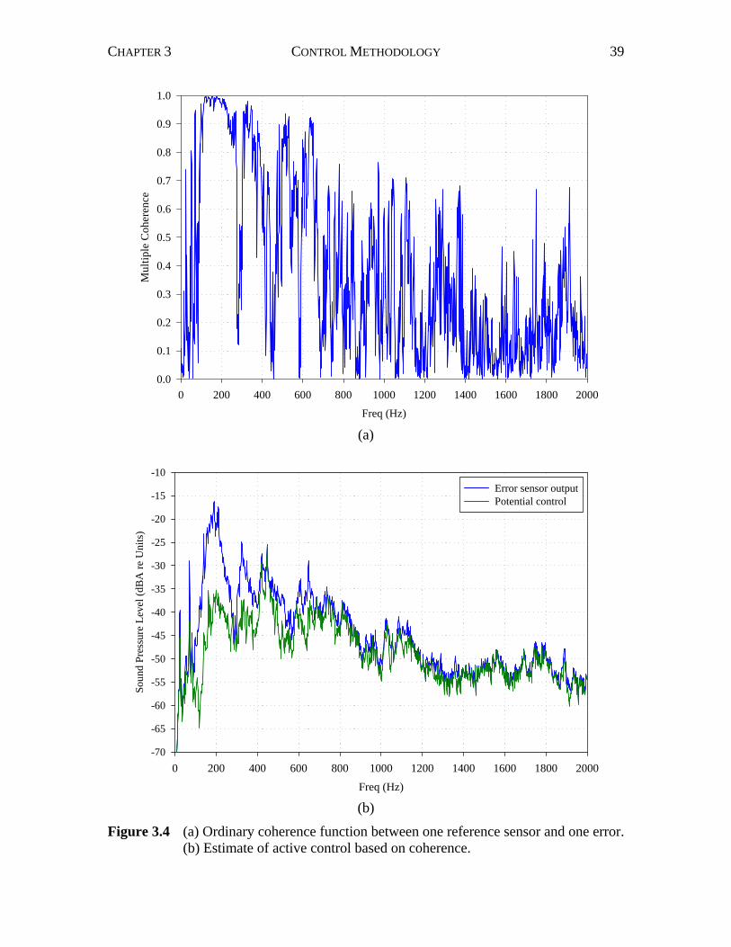
CHAPTER 3 CONTROL METHODOLOGY 39
Freq (Hz)
0 200 400 600 800 1000 1200 1400 1600 1800 2000
Mul
tiple
Coh
eren
ce
0.0
0.1
0.2
0.3
0.4
0.5
0.6
0.7
0.8
0.9
1.0
(a)
Freq (Hz)0 200 400 600 800 1000 1200 1400 1600 1800 2000
Soun
d Pr
essu
re L
evel
(dB
A re
Uni
ts)
-70
-65
-60
-55
-50
-45
-40
-35
-30
-25
-20
-15
-10Error sensor outputPotential control
(b)
Figure 3.4 (a) Ordinary coherence function between one reference sensor and one error. (b) Estimate of active control based on coherence.
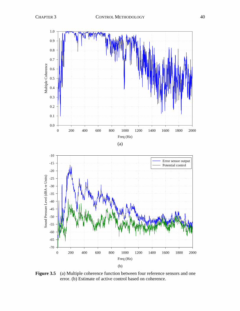
CHAPTER 3 CONTROL METHODOLOGY 40
Freq (Hz)
0 200 400 600 800 1000 1200 1400 1600 1800 2000
Mul
tiple
Coh
eren
ce
0.0
0.1
0.2
0.3
0.4
0.5
0.6
0.7
0.8
0.9
1.0
(a)
Freq (Hz)0 200 400 600 800 1000 1200 1400 1600 1800 2000
Soun
d Pr
essu
re L
evel
(dB
A re
Uni
ts)
-70
-65
-60
-55
-50
-45
-40
-35
-30
-25
-20
-15
-10Error sensor outputPotential control
(b)
Figure 3.5 (a) Multiple coherence function between four reference sensors and one error. (b) Estimate of active control based on coherence.
41
Chapter 4 Test Methodology and Experimental Components 4.1 INTRODUCTION The interior noise within an aircraft cabin is the product of three primary noise sources:
engine noise, noise from structural vibrations induced from wing mounting and
reciprocating engines, and aerodynamic noise. This research focused on the control of
aerodynamic noise or, more specifically, turbulent boundary layer noise in the passenger
cabin. A schematic showing the concepts involved in the control of interior cabin noise
using smart foam elements can be seen in figure 4.1. As shown, an aerodynamic flow
excites the exterior fuselage panels of an aircraft whose vibration then radiates noise into
the cabin. The control concept is to position an array of smart foam actuators between
the fuselage skin and interior trim panel of the aircraft. These actuators act as secondary
noise sources that destructively interfere with the disturbance and reduce the overall
QuietZoneQuietZone
Turbulence
Radiated Cabin Noise
Floor
Aircraft Fuselage
Smart FoamActuators
Fuselage Cross-Section
Anti-Noise
Fuselage Skin Excited by Flow
Trim Panel
Figure 4.1 Schematic of interior noise control using smart foam actuators.
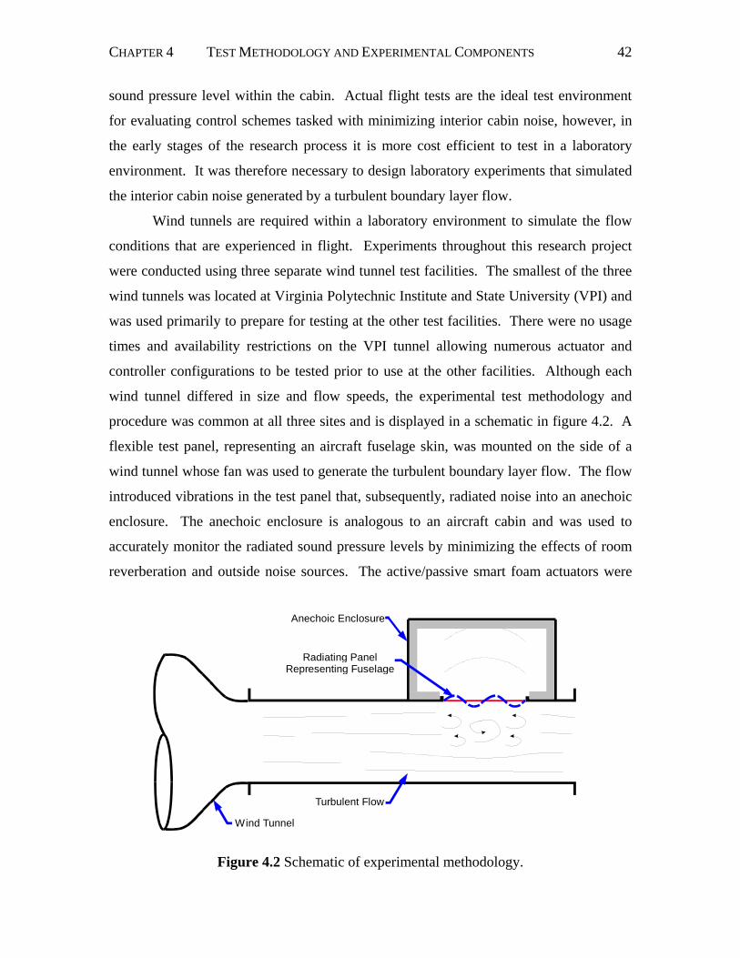
CHAPTER 4 TEST METHODOLOGY AND EXPERIMENTAL COMPONENTS 42
sound pressure level within the cabin. Actual flight tests are the ideal test environment
for evaluating control schemes tasked with minimizing interior cabin noise, however, in
the early stages of the research process it is more cost efficient to test in a laboratory
environment. It was therefore necessary to design laboratory experiments that simulated
the interior cabin noise generated by a turbulent boundary layer flow.
Wind tunnels are required within a laboratory environment to simulate the flow
conditions that are experienced in flight. Experiments throughout this research project
were conducted using three separate wind tunnel test facilities. The smallest of the three
wind tunnels was located at Virginia Polytechnic Institute and State University (VPI) and
was used primarily to prepare for testing at the other test facilities. There were no usage
times and availability restrictions on the VPI tunnel allowing numerous actuator and
controller configurations to be tested prior to use at the other facilities. Although each
wind tunnel differed in size and flow speeds, the experimental test methodology and
procedure was common at all three sites and is displayed in a schematic in figure 4.2. A
flexible test panel, representing an aircraft fuselage skin, was mounted on the side of a
wind tunnel whose fan was used to generate the turbulent boundary layer flow. The flow
introduced vibrations in the test panel that, subsequently, radiated noise into an anechoic
enclosure. The anechoic enclosure is analogous to an aircraft cabin and was used to
accurately monitor the radiated sound pressure levels by minimizing the effects of room
reverberation and outside noise sources. The active/passive smart foam actuators were
Figure 4.2 Schematic of experimental methodology.
Turbulent Flow
Radiating PanelRepresenting Fuselage
Anechoic Enclosure
Wind Tunnel
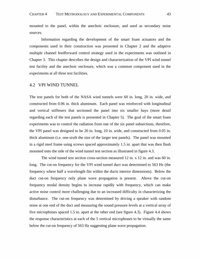
CHAPTER 4 TEST METHODOLOGY AND EXPERIMENTAL COMPONENTS 43
mounted to the panel, within the anechoic enclosure, and used as secondary noise
sources.
Information regarding the development of the smart foam actuators and the
components used in their construction was presented in Chapter 2 and the adaptive
multiple channel feedforward control strategy used in the experiments was outlined in
Chapter 3. This chapter describes the design and characterization of the VPI wind tunnel
test facility and the anechoic enclosure, which was a common component used in the
experiments at all three test facilities.
4.2 VPI WIND TUNNEL The test panels for both of the NASA wind tunnels were 60 in. long, 20 in. wide, and
constructed from 0.06 in. thick aluminum. Each panel was reinforced with longitudinal
and vertical stiffeners that sectioned the panel into six smaller bays (more detail
regarding each of the test panels is presented in Chapter 5). The goal of the smart foam
experiments was to control the radiation from one of the six panel subsections, therefore,
the VPI panel was designed to be 20 in. long, 10 in. wide, and constructed from 0.05 in.
thick aluminum (i.e. one-sixth the size of the larger test panels). The panel was mounted
in a rigid steel frame using screws spaced approximately 1.5 in. apart that was then flush
mounted onto the side of the wind tunnel test section as illustrated in figure 4.3.
The wind tunnel test section cross-section measured 12 in. x 12 in. and was 60 in.
long. The cut-on frequency for the VPI wind tunnel duct was determined to 563 Hz (the
frequency where half a wavelength fits within the ducts interior dimensions). Below the
duct cut-on frequency only plane wave propagation is present. Above the cut-on
frequency modal density begins to increase rapidly with frequency, which can make
active noise control more challenging due to an increased difficulty in characterizing the
disturbance. The cut-on frequency was determined by driving a speaker with random
noise at one end of the duct and measuring the sound pressure levels at a vertical array of
five microphones spaced 1.5 in. apart at the other end (see figure 4.3). Figure 4.4 shows
the response characteristics at each of the 5 vertical microphones to be virtually the same
below the cut-on frequency of 563 Hz suggesting plane wave propagation.
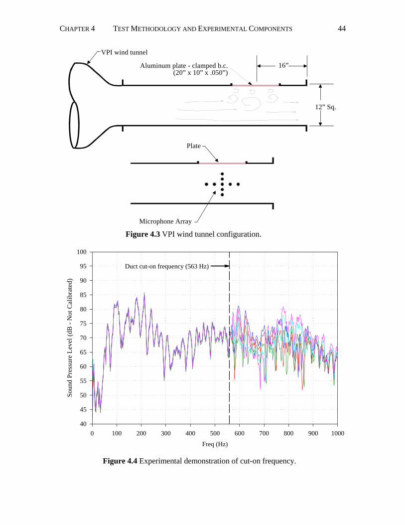
CHAPTER 4 TEST METHODOLOGY AND EXPERIMENTAL COMPONENTS 44
VPI wind tunnel
Aluminum plate - clamped b.c.(20” x 10” x .050”)
16”
12” Sq.
Plate
Microphone Array
Figure 4.3 VPI wind tunnel configuration.
Freq (Hz)
0 100 200 300 400 500 600 700 800 900 1000
Soun
d Pr
essu
re L
evel
(dB
- N
ot C
alib
rate
d)
40
45
50
55
60
65
70
75
80
85
90
95
100
Duct cut-on frequency (563 Hz)
Figure 4.4 Experimental demonstration of cut-on frequency.
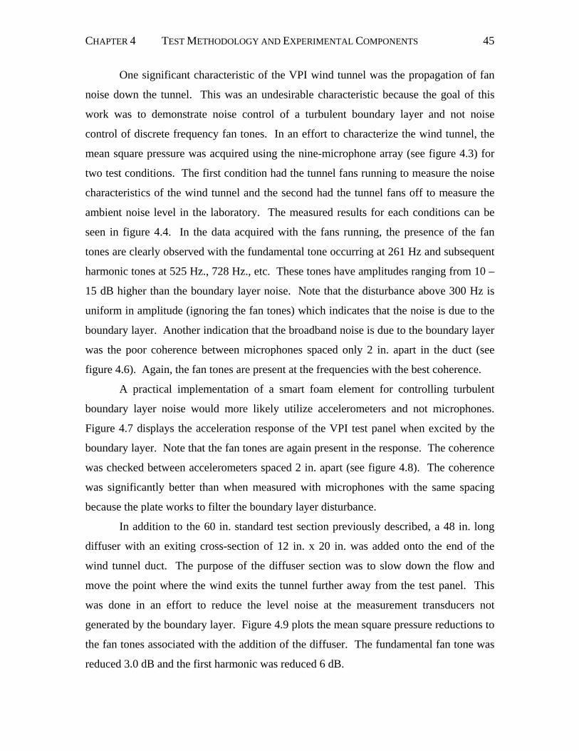
CHAPTER 4 TEST METHODOLOGY AND EXPERIMENTAL COMPONENTS 45
One significant characteristic of the VPI wind tunnel was the propagation of fan
noise down the tunnel. This was an undesirable characteristic because the goal of this
work was to demonstrate noise control of a turbulent boundary layer and not noise
control of discrete frequency fan tones. In an effort to characterize the wind tunnel, the
mean square pressure was acquired using the nine-microphone array (see figure 4.3) for
two test conditions. The first condition had the tunnel fans running to measure the noise
characteristics of the wind tunnel and the second had the tunnel fans off to measure the
ambient noise level in the laboratory. The measured results for each conditions can be
seen in figure 4.4. In the data acquired with the fans running, the presence of the fan
tones are clearly observed with the fundamental tone occurring at 261 Hz and subsequent
harmonic tones at 525 Hz., 728 Hz., etc. These tones have amplitudes ranging from 10 –
15 dB higher than the boundary layer noise. Note that the disturbance above 300 Hz is
uniform in amplitude (ignoring the fan tones) which indicates that the noise is due to the
boundary layer. Another indication that the broadband noise is due to the boundary layer
was the poor coherence between microphones spaced only 2 in. apart in the duct (see
figure 4.6). Again, the fan tones are present at the frequencies with the best coherence.
A practical implementation of a smart foam element for controlling turbulent
boundary layer noise would more likely utilize accelerometers and not microphones.
Figure 4.7 displays the acceleration response of the VPI test panel when excited by the
boundary layer. Note that the fan tones are again present in the response. The coherence
was checked between accelerometers spaced 2 in. apart (see figure 4.8). The coherence
was significantly better than when measured with microphones with the same spacing
because the plate works to filter the boundary layer disturbance.
In addition to the 60 in. standard test section previously described, a 48 in. long
diffuser with an exiting cross-section of 12 in. x 20 in. was added onto the end of the
wind tunnel duct. The purpose of the diffuser section was to slow down the flow and
move the point where the wind exits the tunnel further away from the test panel. This
was done in an effort to reduce the level noise at the measurement transducers not
generated by the boundary layer. Figure 4.9 plots the mean square pressure reductions to
the fan tones associated with the addition of the diffuser. The fundamental fan tone was
reduced 3.0 dB and the first harmonic was reduced 6 dB.
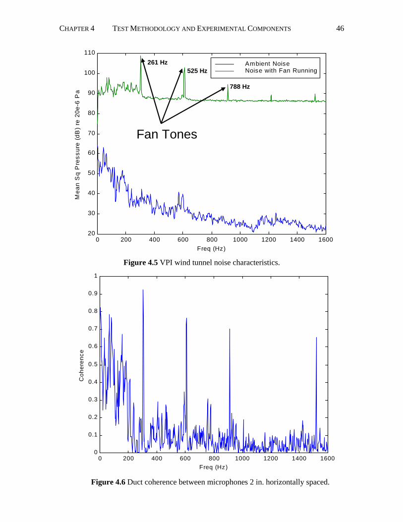
CHAPTER 4 TEST METHODOLOGY AND EXPERIMENTAL COMPONENTS 46
0 200 400 600 800 1000 1200 1400 160020
30
40
50
60
70
80
90
100
110
Freq (Hz)
Mea
n S
q P
ress
ure
(dB
) re
20e
-6 P
a
Ambient Noise Noise with Fan Running
Fan Tones
261 Hz525 Hz
788 Hz
Figure 4.6 Duct coherence between microphones 2 in. horizontally spaced.
0 200 400 600 800 1000 1200 1400 16000
0.1
0.2
0.3
0.4
0.5
0.6
0.7
0.8
0.9
1
Freq (Hz)
Coh
eren
ce
Figure 4.5 VPI wind tunnel noise characteristics.

CHAPTER 4 TEST METHODOLOGY AND EXPERIMENTAL COMPONENTS 47
0 200 400 600 800 1000 1200 1400 1600 1800 2000-80
-70
-60
-50
-40
-30
-20
-10
0
10
Freq (Hz)
Acc
eler
atio
n (d
B)
re 1
g
0 200 400 600 800 1000 1200 1400 1600 1800 20000
0.1
0.2
0.3
0.4
0.5
0.6
0.7
0.8
0.9
1
Freq (Hz)
Coh
eren
ce
Figure 4.7 VPI test plate accelerometer response characteristics.
Figure 4.8 VPI plate coherence between accelerometers 2 in. apart.

CHAPTER 4 TEST METHODOLOGY AND EXPERIMENTAL COMPONENTS 48
Additional effort was made to reduce the fan tone levels with the addition of an
array of Herschel-Quincke (HQ) tubes as seen in figure 4.10. HQ tubes are passive noise
attenuation devices that have the ability to attenuate the harmonics of a fundamental
frequency. The device is a hollow tube with two ends that each attach to the side wall of
a main duct with the two ends aligned in the direction of the flow. The incident acoustic
wave divides at the first intersection with the HQ tube and recombines with the incident
wave downstream. The difference in path length results in a phase shift between the two
waves that result in sound attenuation at a select number of frequencies. Factors such as
the length of tube, cross-sectional area of the tube, and distance between inlet and outlet
openings are all parameters that can be used to tune the performance of a HQ tube. The
tuning and implementation of Herschel-Quincke tubes was not a major focus of the
project, but with minimal tuning and adjustment the levels of the fan tones were reduced
by approximately 4 dB at both the fundamental and first harmonic frequency.
0 200 400 600 800 1000 1200 1400 1600 1800 200010
20
30
40
50
60
70
80
Freq (Hz)
Mea
n S
q P
ress
ure
(dB
) re
20e-
6 P
a
No DiffuserDiffuser
61.1 Hz
67.1 Hz67.1 Hz
70.1 Hz
Figure 4.9 Fan tone reduction from diffuser.
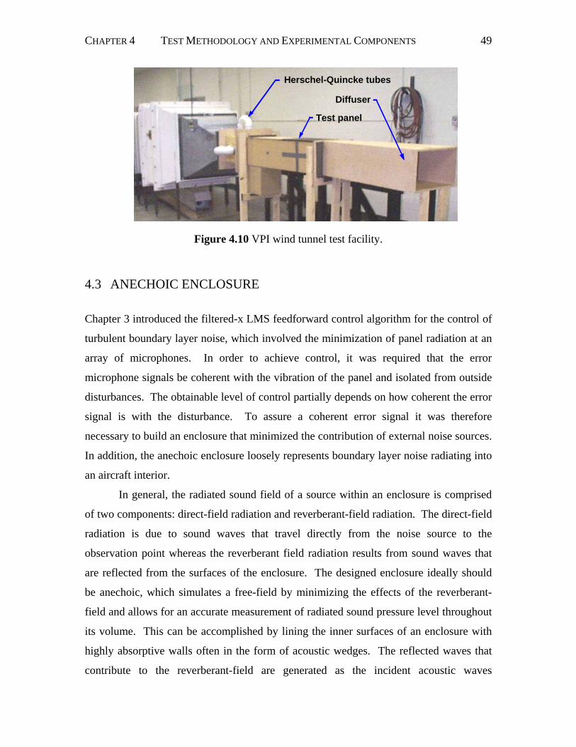
CHAPTER 4 TEST METHODOLOGY AND EXPERIMENTAL COMPONENTS 49
4.3 ANECHOIC ENCLOSURE Chapter 3 introduced the filtered-x LMS feedforward control algorithm for the control of
turbulent boundary layer noise, which involved the minimization of panel radiation at an
array of microphones. In order to achieve control, it was required that the error
microphone signals be coherent with the vibration of the panel and isolated from outside
disturbances. The obtainable level of control partially depends on how coherent the error
signal is with the disturbance. To assure a coherent error signal it was therefore
necessary to build an enclosure that minimized the contribution of external noise sources.
In addition, the anechoic enclosure loosely represents boundary layer noise radiating into
an aircraft interior.
In general, the radiated sound field of a source within an enclosure is comprised
of two components: direct-field radiation and reverberant-field radiation. The direct-field
radiation is due to sound waves that travel directly from the noise source to the
observation point whereas the reverberant field radiation results from sound waves that
are reflected from the surfaces of the enclosure. The designed enclosure ideally should
be anechoic, which simulates a free-field by minimizing the effects of the reverberant-
field and allows for an accurate measurement of radiated sound pressure level throughout
its volume. This can be accomplished by lining the inner surfaces of an enclosure with
highly absorptive walls often in the form of acoustic wedges. The reflected waves that
contribute to the reverberant-field are generated as the incident acoustic waves
Herschel-Quincke tubes
Test panel
Diffuser
Figure 4.10 VPI wind tunnel test facility.
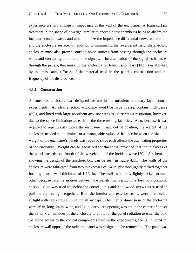
CHAPTER 4 TEST METHODOLOGY AND EXPERIMENTAL COMPONENTS 50
experience a sharp change in impedance at the wall of the enclosure. A foam surface
treatment in the shape of a wedge (similar to anechoic test chambers) helps to absorb the
incident acoustic waves and also minimize the impedance differential between the room
and the enclosure surface. In addition to minimizing the reverberant field, the anechoic
enclosure must also prevent outside noise sources from passing through the enclosure
walls and corrupting the microphone signals. The attenuation of the signal as it passes
through the panels, that make up the enclosure, or transmission loss (TL), is established
by the mass and stiffness of the material used in the panel’s construction and the
frequency of the disturbance.
4.3.1 Construction
An anechoic enclosure was designed for use in the turbulent boundary layer control
experiments. An ideal anechoic enclosure would be large in size, contain thick dense
walls, and lined with large absorbent acoustic wedges. Size was a restriction, however,
due to the space limitations at each of the three testing facilities. Also, because it was
required to repetitiously move the enclosure in and out of position, the weight of the
enclosure needed to be limited to a manageable value. A balance between the size and
weight of the enclosure’s panels was required since each affects the attenuating properties
of the enclosure. Weight can be sacrificed for thickness, provided that the thickness of
the panel exceeds one-fourth of the wavelength of the incident wave [50]. A schematic
showing the design of the anechoic box can be seen in figure 4.11. The walls of the
enclosure were fabricated from two thicknesses of 3/4 in. plywood lightly tacked together
forming a total wall thickness of 1-1/2 in. The walls were only lightly tacked to each
other because relative motion between the panels will result in a loss of vibrational
energy. Glue was used to anchor the corner joints and 3 in. wood screws were used to
pull the corners tight together. Both the interior and exterior seams were then sealed
airtight with caulk thus eliminating all air gaps. The interior dimensions of the enclosure
were 36 in. long, 24 in. wide, and 24 in. deep. An opening was cut in the center of one of
the 36 in. x 24 in. sides of the enclosure to allow for the panel radiation to enter the box.
To allow access to the control components used in the experiments, the 36 in. x 24 in.
enclosure wall opposite the radiating panel was designed to be removable. The panel was
CHAPTER 4 TEST METHODOLOGY AND EXPERIMENTAL COMPONENTS 51
sealed with 1/2 in. wide and 1/2 in. thick airtight foam tape and held closed with six
compression latches during tunnel operation.
Structural excitation of the anechoic enclosure induced through contact with the
vibrating wind tunnel would introduce additional noise into the system. Two strips of the
same 1/2 in. wide and 1/2 in. thick foam tape were positioned around the panel opening
between the wall of the wind tunnel and anechoic box as an attempt to isolate the tunnel
vibration. Accelerometers were mounted to the enclosure and the wind tunnel and the
relative vibration levels were compared. It was concluded that the vibration transmission
was sufficiently low as to not induce an additional noise source of any significance. The
interior walls of the enclosure were lined with SONEXsuper™ wedges made from
wiltec®, a lightweight, semi-flexible, low-density foam [51]. Each foam block measured
12 in. square and contained three 6 in. wedges. The wedge squares were arranged in an
alternating pattern, as is conventional in anechoic enclosure design, and were mitered to
fit snug within each corner so that the entire interior surface was coated with the acoustic
material.
4.3.2 Characterization
24”
36”
24”
Compression latches
Air tight foam seal
2 x 3/4” thick plywood walls
6” foam wedges
Opening for plate radiation
Figure 4.11 Anechoic enclosure.
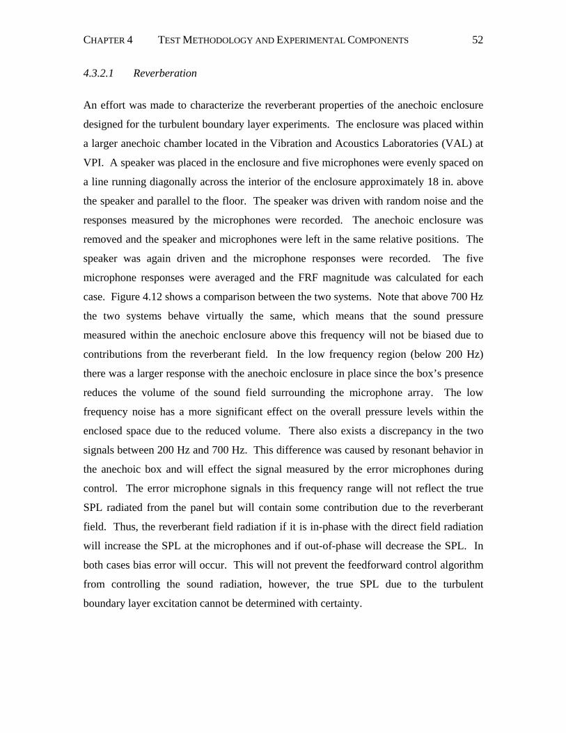
CHAPTER 4 TEST METHODOLOGY AND EXPERIMENTAL COMPONENTS 52
4.3.2.1 Reverberation
An effort was made to characterize the reverberant properties of the anechoic enclosure
designed for the turbulent boundary layer experiments. The enclosure was placed within
a larger anechoic chamber located in the Vibration and Acoustics Laboratories (VAL) at
VPI. A speaker was placed in the enclosure and five microphones were evenly spaced on
a line running diagonally across the interior of the enclosure approximately 18 in. above
the speaker and parallel to the floor. The speaker was driven with random noise and the
responses measured by the microphones were recorded. The anechoic enclosure was
removed and the speaker and microphones were left in the same relative positions. The
speaker was again driven and the microphone responses were recorded. The five
microphone responses were averaged and the FRF magnitude was calculated for each
case. Figure 4.12 shows a comparison between the two systems. Note that above 700 Hz
the two systems behave virtually the same, which means that the sound pressure
measured within the anechoic enclosure above this frequency will not be biased due to
contributions from the reverberant field. In the low frequency region (below 200 Hz)
there was a larger response with the anechoic enclosure in place since the box’s presence
reduces the volume of the sound field surrounding the microphone array. The low
frequency noise has a more significant effect on the overall pressure levels within the
enclosed space due to the reduced volume. There also exists a discrepancy in the two
signals between 200 Hz and 700 Hz. This difference was caused by resonant behavior in
the anechoic box and will effect the signal measured by the error microphones during
control. The error microphone signals in this frequency range will not reflect the true
SPL radiated from the panel but will contain some contribution due to the reverberant
field. Thus, the reverberant field radiation if it is in-phase with the direct field radiation
will increase the SPL at the microphones and if out-of-phase will decrease the SPL. In
both cases bias error will occur. This will not prevent the feedforward control algorithm
from controlling the sound radiation, however, the true SPL due to the turbulent
boundary layer excitation cannot be determined with certainty.
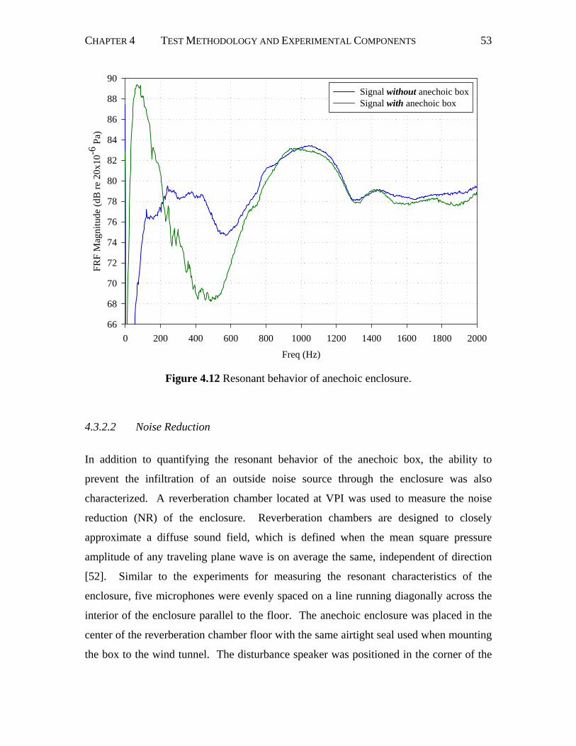
CHAPTER 4 TEST METHODOLOGY AND EXPERIMENTAL COMPONENTS 53
4.3.2.2 Noise Reduction
In addition to quantifying the resonant behavior of the anechoic box, the ability to
prevent the infiltration of an outside noise source through the enclosure was also
characterized. A reverberation chamber located at VPI was used to measure the noise
reduction (NR) of the enclosure. Reverberation chambers are designed to closely
approximate a diffuse sound field, which is defined when the mean square pressure
amplitude of any traveling plane wave is on average the same, independent of direction
[52]. Similar to the experiments for measuring the resonant characteristics of the
enclosure, five microphones were evenly spaced on a line running diagonally across the
interior of the enclosure parallel to the floor. The anechoic enclosure was placed in the
center of the reverberation chamber floor with the same airtight seal used when mounting
the box to the wind tunnel. The disturbance speaker was positioned in the corner of the
Freq (Hz)
0 200 400 600 800 1000 1200 1400 1600 1800 2000
FRF
Mag
nitu
de (d
B re
20x
10-6
Pa)
66
68
70
72
74
76
78
80
82
84
86
88
90Signal without anechoic boxSignal with anechoic box
Figure 4.12 Resonant behavior of anechoic enclosure.
CHAPTER 4 TEST METHODOLOGY AND EXPERIMENTAL COMPONENTS 54
reverberation chamber in order to maximize its radiation efficiency. The SPL’s were
recorded with and without the anechoic box in place and can be seen in figure 4.13(a).
The difference in the two traces was the NR induced by the anechoic enclosure and is
displayed in third-octave bands in figure 4.13(b). Note the increase in NR at the higher
frequencies. This occurs because the NR of an enclosure is a function of not only the
mass and thickness of the panels that make up the enclosure but also the frequency of the
disturbance.
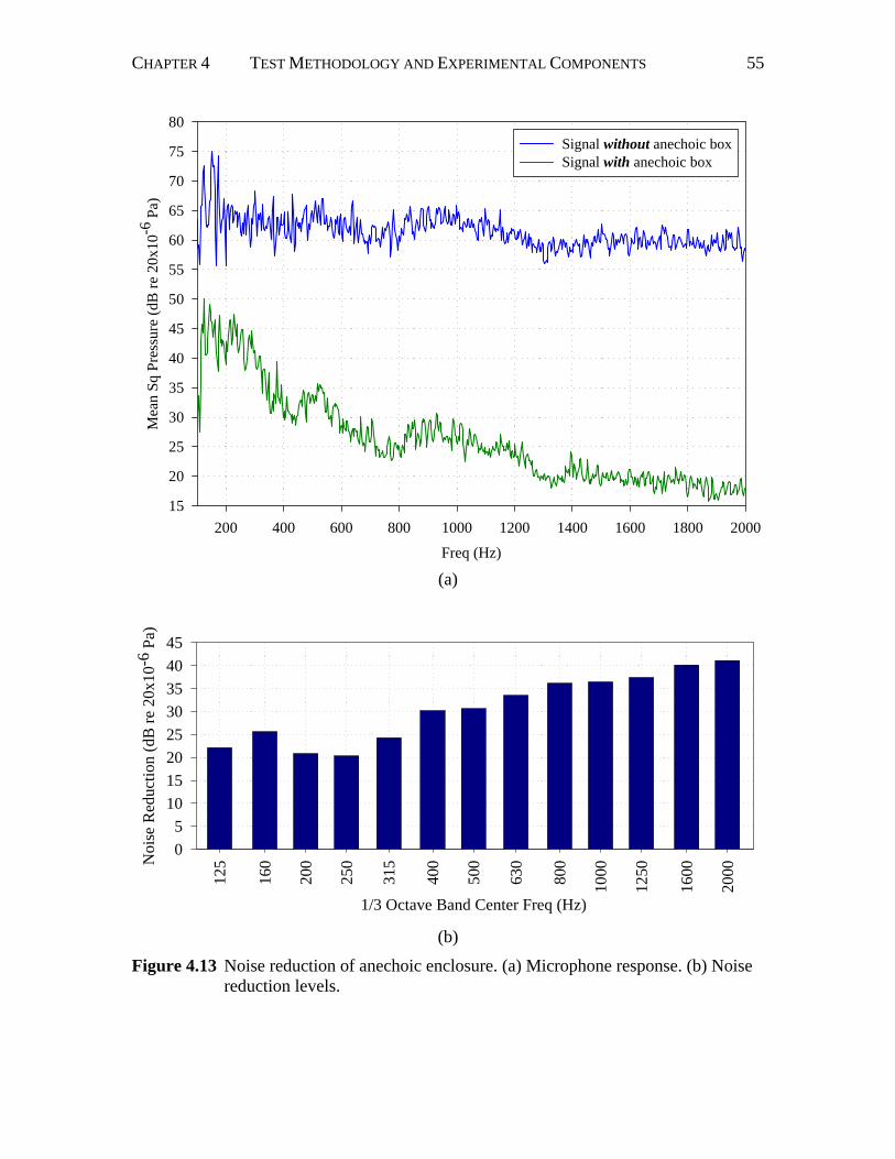
CHAPTER 4 TEST METHODOLOGY AND EXPERIMENTAL COMPONENTS 55
Freq (Hz)
200 400 600 800 1000 1200 1400 1600 1800 2000
Mea
n Sq
Pre
ssur
e (d
B re
20x
10-6
Pa)
15
20
25
30
35
40
45
50
55
60
65
70
75
80Signal without anechoic boxSignal with anechoic box
(a)
1/3 Octave Band Center Freq (Hz)
125
160
200
250
315
400
500
630
800
1000
1250
1600
2000
Noi
se R
educ
tion
(dB
re 2
0x10
-6 P
a)
05
1015202530354045
(b)
Figure 4.13 Noise reduction of anechoic enclosure. (a) Microphone response. (b) Noise reduction levels.
56
Chapter 5 Experimental Results 5.1 INTRODUCTION It has been the goal of this research to demonstrate the active control of sound radiation
from a panel that has been excited with a turbulent boundary layer disturbance. The
Structural Acoustics Branch of the NASA Langley Research Center (LaRC) has funded
this work as part of a subprogram of the Advanced Subsonic Technology noise reduction
program concerned with interior noise. Historically, much of the work in the area of
aircraft interior noise has been focused on passive treatments and active control
techniques that utilize speakers or input forces as control sources (see Chapter 1). These
techniques are often characterized as point approaches since the interaction between the
control elements and noise source is localized. Recognizing the limitations of these noise
control methods has prompted researchers to consider new control techniques that take
advantage of both passive and active control components. The hybrid, active/passive
technique of smart foam used in this research (see Chapter 2) is considered a smart skin
or a fully distributed noise control approach since the entire noise source is treated with
the combined active and passive elements of the device. Smart foam is just one of the
many methods being examined for controlling the aircraft interior noise problem.
The present smart foam project has been conducted in parallel with a separate
NASA LaRC project also tasked with the active control of turbulent boundary layer noise
using piezoceramic actuators attached to a panel. Together these two project interests
helped to determine the timetable and operating conditions for each set of experiments.
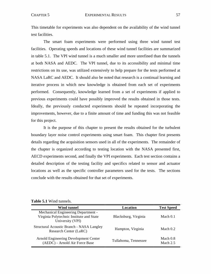
CHAPTER 5 EXPERIMENTAL RESULTS 57
This timetable for experiments was also dependent on the availability of the wind tunnel
test facilities.
The smart foam experiments were performed using three wind tunnel test
facilities. Operating speeds and locations of these wind tunnel facilities are summarized
in table 5.1. The VPI wind tunnel is a much smaller and more unrefined than the tunnels
at both NASA and AEDC. The VPI tunnel, due to its accessibility and minimal time
restrictions on its use, was utilized extensively to help prepare for the tests performed at
NASA LaRC and AEDC. It should also be noted that research is a continual learning and
iterative process in which new knowledge is obtained from each set of experiments
performed. Consequently, knowledge learned from a set of experiments if applied to
previous experiments could have possibly improved the results obtained in those tests.
Ideally, the previously conducted experiments should be repeated incorporating the
improvements, however, due to a finite amount of time and funding this was not feasible
for this project.
It is the purpose of this chapter to present the results obtained for the turbulent
boundary layer noise control experiments using smart foam. This chapter first presents
details regarding the acquisition sensors used in all of the experiments. The remainder of
the chapter is organized according to testing location with the NASA presented first,
AECD experiments second, and finally the VPI experiments. Each test section contains a
detailed description of the testing facility and specifics related to sensor and actuator
locations as well as the specific controller parameters used for the tests. The sections
conclude with the results obtained for that set of experiments.
Table 5.1 Wind tunnels. Wind tunnel Location Test Speed
Mechanical Engineering Department -Virginia Polytechnic Institute and State
University (VPI)Blacksburg, Virginia Mach 0.1
Structural Acoustic Branch - NASA LangleyResearch Center (LaRC) Hampton, Virginia Mach 0.2
Arnold Engineering Development Center(AEDC) - Arnold Air Force Base Tullahoma, Tennessee Mach 0.8
Mach 2.5
CHAPTER 5 EXPERIMENTAL RESULTS 58
5.2 ACQUISITION SENSORS Chapter 3 presented the multi-channel filtered-x LMS feedforward control algorithm used
in the smart foam turbulent boundary layer experiments. This methodology can be used
to generate multiple control signals based on information supplied by arrays of both error
and reference signals. This section will provide specifics regarding the transducers
chosen to serve as error and reference signals and the reason each type was chosen. The
transducers that were used as error and reference signals were common to all experiments
performed at each of the three test locations. Characteristics specific to each set of
experiments will be presented in the measurement setup section for each test location.
As discussed in Chapter 2, the output signal of the system plant is the summation
of both the actual disturbance signal and the secondary actuator signals generated by the
controller. It is the goal of the controller to adjust the magnitude and phase of the
secondary control signal so that by superposition the error signal is minimized. For the
smart foam experiments performed in this research, the error signals were generated
using microphones. Microphones were chosen as the minimization criteria because it
was the principal goal of the work to reduce the interior cabin noise perceived by an
aircraft crew. PCB Acousticel microphones (Model TMS-130B) connected to a PCB
Acousticel signal conditioner (573 Series) were used in all experiments.
In the filtered-x LMS feedforward control algorithm the reference signals are used
to provide the controller with knowledge of the disturbance. PCB piezoelectric ICP
accelerometers (Model 352A10) were used for all experiments and mounted directly to
the test panel surface. Each accelerometer weighed approximately 0.7 grams making the
combined weight of all reference accelerometers only 0.6% of the NASA and VPI test
panel weight and 1% of the AECD test panel weight. These percentages are based on the
weight of the panel test section exclusively and do not include the weight of the stringers
and frames used to stiffen the NASA & AEDC test panels. Each accelerometer was
connected to a twelve-channel PCB signal conditioner (Model 483B07) with adjustable
gains for each channel that were set in order to take advantage of the dynamic range of
the input A/D converters. Accelerometers were chosen because the controller requires
sufficient time advance in order to determine and induce the secondary control signals
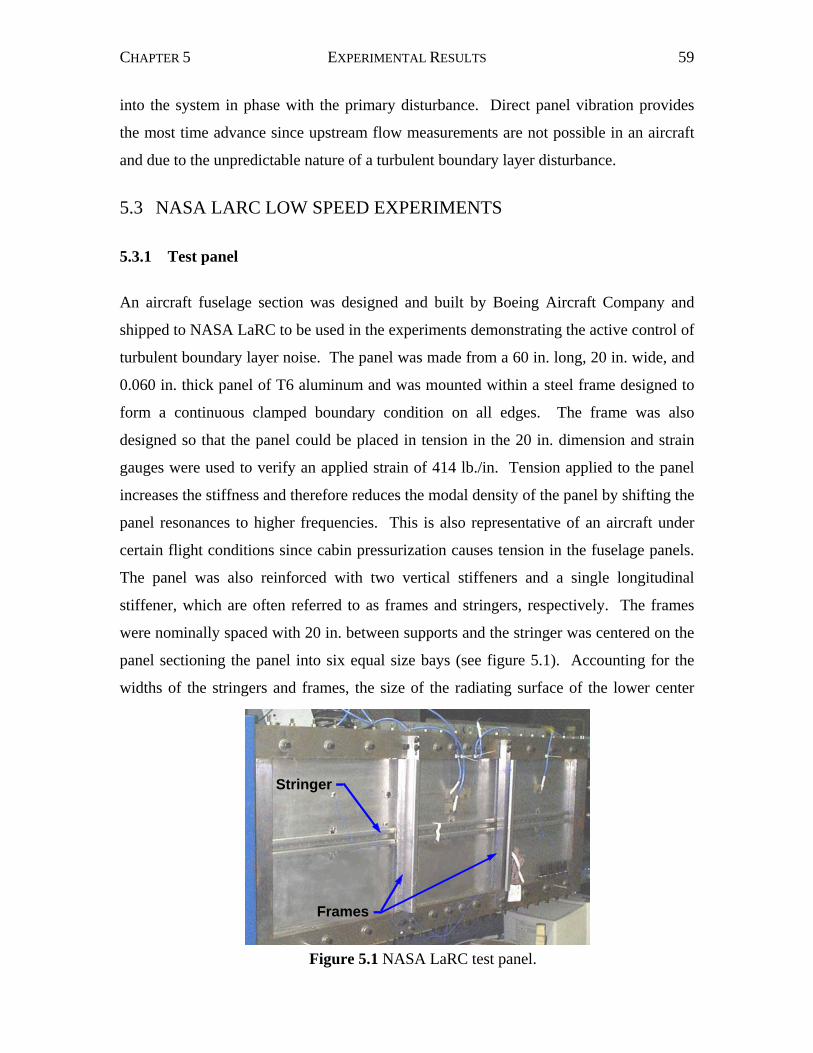
CHAPTER 5 EXPERIMENTAL RESULTS 59
into the system in phase with the primary disturbance. Direct panel vibration provides
the most time advance since upstream flow measurements are not possible in an aircraft
and due to the unpredictable nature of a turbulent boundary layer disturbance.
5.3 NASA LARC LOW SPEED EXPERIMENTS 5.3.1 Test panel
An aircraft fuselage section was designed and built by Boeing Aircraft Company and
shipped to NASA LaRC to be used in the experiments demonstrating the active control of
turbulent boundary layer noise. The panel was made from a 60 in. long, 20 in. wide, and
0.060 in. thick panel of T6 aluminum and was mounted within a steel frame designed to
form a continuous clamped boundary condition on all edges. The frame was also
designed so that the panel could be placed in tension in the 20 in. dimension and strain
gauges were used to verify an applied strain of 414 lb./in. Tension applied to the panel
increases the stiffness and therefore reduces the modal density of the panel by shifting the
panel resonances to higher frequencies. This is also representative of an aircraft under
certain flight conditions since cabin pressurization causes tension in the fuselage panels.
The panel was also reinforced with two vertical stiffeners and a single longitudinal
stiffener, which are often referred to as frames and stringers, respectively. The frames
were nominally spaced with 20 in. between supports and the stringer was centered on the
panel sectioning the panel into six equal size bays (see figure 5.1). Accounting for the
widths of the stringers and frames, the size of the radiating surface of the lower center
Stringer
Frames
Figure 5.1 NASA LaRC test panel.
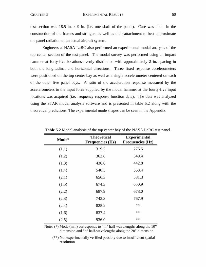
CHAPTER 5 EXPERIMENTAL RESULTS 60
test section was 18.5 in. x 9 in. (i.e. one sixth of the panel). Care was taken in the
construction of the frames and stringers as well as their attachment to best approximate
the panel radiation of an actual aircraft system.
Engineers at NASA LaRC also performed an experimental modal analysis of the
top center section of the test panel. The modal survey was performed using an impact
hammer at forty-five locations evenly distributed with approximately 2 in. spacing in
both the longitudinal and horizontal directions. Three fixed response accelerometers
were positioned on the top center bay as well as a single accelerometer centered on each
of the other five panel bays. A ratio of the acceleration response measured by the
accelerometers to the input force supplied by the modal hammer at the fourty-five input
locations was acquired (i.e. frequency response function data). The data was analyzed
using the STAR modal analysis software and is presented in table 5.2 along with the
theoretical predictions. The experimental mode shapes can be seen in the Appendix.
Table 5.2 Modal analysis of the top center bay of the NASA LaRC test panel.
Mode* TheoreticalFrequencies (Hz)
ExperimentalFrequencies (Hz)
(1,1) 319.2 275.5
(1,2) 362.8 349.4
(1,3) 436.6 442.8
(1,4) 540.5 553.4
(2.1) 656.3 581.3
(1,5) 674.3 650.9
(2,2) 687.9 678.0
(2,3) 743.3 767.9
(2,4) 825.2 **
(1,6) 837.4 **
(2,5) 936.0 **Note: (*) Mode (m,n) corresponds to “m” half-wavelengths along the 10”
dimension and “n” half-wavelengths along the 20” dimension.
(**) Not experimentally verified possibly due to insufficient spatialresolution
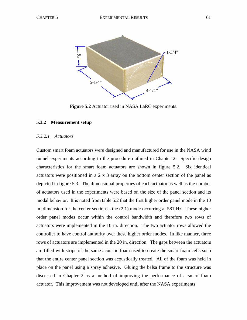
CHAPTER 5 EXPERIMENTAL RESULTS 61
5.3.2 Measurement setup
5.3.2.1 Actuators
Custom smart foam actuators were designed and manufactured for use in the NASA wind
tunnel experiments according to the procedure outlined in Chapter 2. Specific design
characteristics for the smart foam actuators are shown in figure 5.2. Six identical
actuators were positioned in a 2 x 3 array on the bottom center section of the panel as
depicted in figure 5.3. The dimensional properties of each actuator as well as the number
of actuators used in the experiments were based on the size of the panel section and its
modal behavior. It is noted from table 5.2 that the first higher order panel mode in the 10
in. dimension for the center section is the (2,1) mode occurring at 581 Hz. These higher
order panel modes occur within the control bandwidth and therefore two rows of
actuators were implemented in the 10 in. direction. The two actuator rows allowed the
controller to have control authority over these higher order modes. In like manner, three
rows of actuators are implemented in the 20 in. direction. The gaps between the actuators
are filled with strips of the same acoustic foam used to create the smart foam cells such
that the entire center panel section was acoustically treated. All of the foam was held in
place on the panel using a spray adhesive. Gluing the balsa frame to the structure was
discussed in Chapter 2 as a method of improving the performance of a smart foam
actuator. This improvement was not developed until after the NASA experiments.
Figure 5.2 Actuator used in NASA LaRC experiments.
5-1/4”
4-1/4”
2”1-3/4”
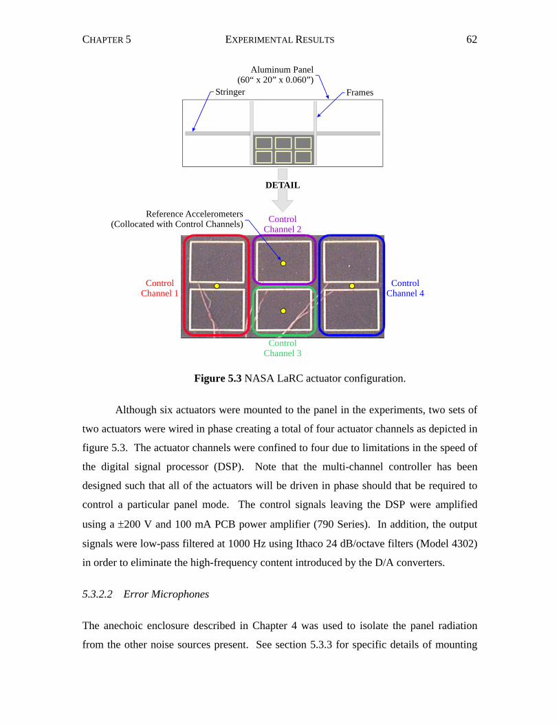
CHAPTER 5 EXPERIMENTAL RESULTS 62
Although six actuators were mounted to the panel in the experiments, two sets of
two actuators were wired in phase creating a total of four actuator channels as depicted in
figure 5.3. The actuator channels were confined to four due to limitations in the speed of
the digital signal processor (DSP). Note that the multi-channel controller has been
designed such that all of the actuators will be driven in phase should that be required to
control a particular panel mode. The control signals leaving the DSP were amplified
using a ±200 V and 100 mA PCB power amplifier (790 Series). In addition, the output
signals were low-pass filtered at 1000 Hz using Ithaco 24 dB/octave filters (Model 4302)
in order to eliminate the high-frequency content introduced by the D/A converters.
5.3.2.2 Error Microphones
The anechoic enclosure described in Chapter 4 was used to isolate the panel radiation
from the other noise sources present. See section 5.3.3 for specific details of mounting
Stringer Frames
Aluminum Panel(60“ x 20” x 0.060”)
DETAIL
ControlChannel 3
ControlChannel 1
ControlChannel 4
ControlChannel 2
Reference Accelerometers(Collocated with Control Channels)
Figure 5.3 NASA LaRC actuator configuration.
CHAPTER 5 EXPERIMENTAL RESULTS 63
the anechoic enclosure. Four error microphones were located within the anechoic box
along the midpoint of each panel edge suspended approximately 20 in. above the panel.
The controller functions by attempting to reduce the radiated sound pressure only at the
error microphones, which can sometimes result in an increase in sound pressure at other
locations. To help monitor the global performance of the controller an additional four
microphones were also distributed 20 in. above the panel in the anechoic box. The
confined physical size of the anechoic enclosure and test facility prevented the use of
additional monitoring microphones.
The poor sound radiation characteristic of a smart foam cell at low frequencies
was addressed in Chapter 2 where the typical radiated sound power of an actuator used in
the NASA LaRC experiments was shown (Small Actuator curve of figure 2.9(a)). The
radiation characteristics of the actuators coupled with the modal properties of the panel
were used to determine the frequency range for control. It was necessary to remove the
low frequency radiation content from the error signals in order to prevent the controller
from driving the actuators in this range, where they have no control authority. If the
control system was allowed to drive the actuators where they were incapable of
generating sufficient sound power (see Chapter 2), then the control system became
unstable and needed to be reset. The lowest frequency that could be tolerated by the
control system was both a function of the radiation characteristic of the smart foam and
the noise content. The value where the instability occurred varied for each test, but
typically the low value of each control band was the lowest frequency that could be
tolerated by the control system. Also, due to the inherent active/passive properties of the
smart foam, the high frequency radiation content was removed (i.e. where the passive
attenuation properties of the smart foam work well). This was accomplished by band-
pass filtering each error channel with two Ithaco filters (Model 4302) connected in series.
The control bandwidth for the NASA LaRC experiments was set to be 400 – 1000 Hz.
5.3.2.3 Reference Accelerometers
The reference signals required for control were provided by four fixed response
accelerometers mounted to the surface of the panel. Again, four was the maximum
number of possible references due to the speed limitations of the DSP. As discussed in
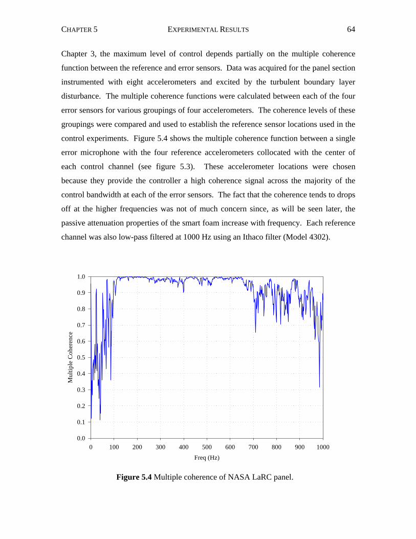
CHAPTER 5 EXPERIMENTAL RESULTS 64
Chapter 3, the maximum level of control depends partially on the multiple coherence
function between the reference and error sensors. Data was acquired for the panel section
instrumented with eight accelerometers and excited by the turbulent boundary layer
disturbance. The multiple coherence functions were calculated between each of the four
error sensors for various groupings of four accelerometers. The coherence levels of these
groupings were compared and used to establish the reference sensor locations used in the
control experiments. Figure 5.4 shows the multiple coherence function between a single
error microphone with the four reference accelerometers collocated with the center of
each control channel (see figure 5.3). These accelerometer locations were chosen
because they provide the controller a high coherence signal across the majority of the
control bandwidth at each of the error sensors. The fact that the coherence tends to drops
off at the higher frequencies was not of much concern since, as will be seen later, the
passive attenuation properties of the smart foam increase with frequency. Each reference
channel was also low-pass filtered at 1000 Hz using an Ithaco filter (Model 4302).
Figure 5.4 Multiple coherence of NASA LaRC panel.
Freq (Hz)
0 100 200 300 400 500 600 700 800 900 1000
Mul
tiple
Coh
eren
ce
0.0
0.1
0.2
0.3
0.4
0.5
0.6
0.7
0.8
0.9
1.0
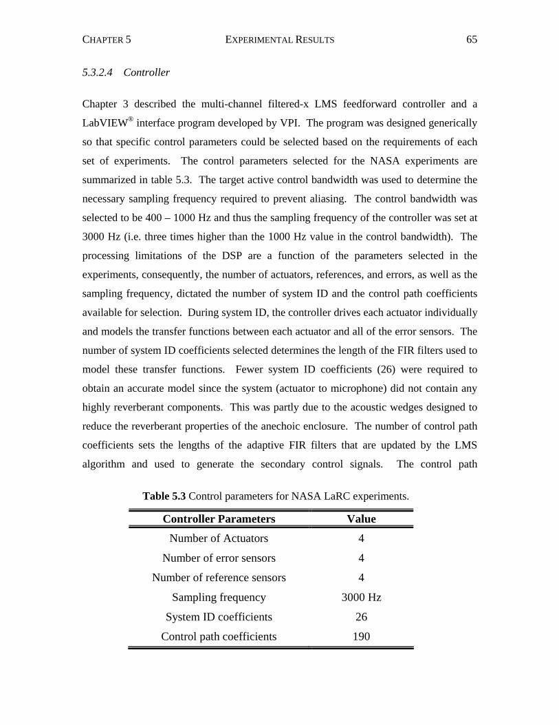
CHAPTER 5 EXPERIMENTAL RESULTS 65
5.3.2.4 Controller
Chapter 3 described the multi-channel filtered-x LMS feedforward controller and a
LabVIEW® interface program developed by VPI. The program was designed generically
so that specific control parameters could be selected based on the requirements of each
set of experiments. The control parameters selected for the NASA experiments are
summarized in table 5.3. The target active control bandwidth was used to determine the
necessary sampling frequency required to prevent aliasing. The control bandwidth was
selected to be 400 – 1000 Hz and thus the sampling frequency of the controller was set at
3000 Hz (i.e. three times higher than the 1000 Hz value in the control bandwidth). The
processing limitations of the DSP are a function of the parameters selected in the
experiments, consequently, the number of actuators, references, and errors, as well as the
sampling frequency, dictated the number of system ID and the control path coefficients
available for selection. During system ID, the controller drives each actuator individually
and models the transfer functions between each actuator and all of the error sensors. The
number of system ID coefficients selected determines the length of the FIR filters used to
model these transfer functions. Fewer system ID coefficients (26) were required to
obtain an accurate model since the system (actuator to microphone) did not contain any
highly reverberant components. This was partly due to the acoustic wedges designed to
reduce the reverberant properties of the anechoic enclosure. The number of control path
coefficients sets the lengths of the adaptive FIR filters that are updated by the LMS
algorithm and used to generate the secondary control signals. The control path
Controller Parameters Value
Number of Actuators 4
Number of error sensors 4
Number of reference sensors 4
Sampling frequency 3000 Hz
System ID coefficients 26
Control path coefficients 190
Table 5.3 Control parameters for NASA LaRC experiments.
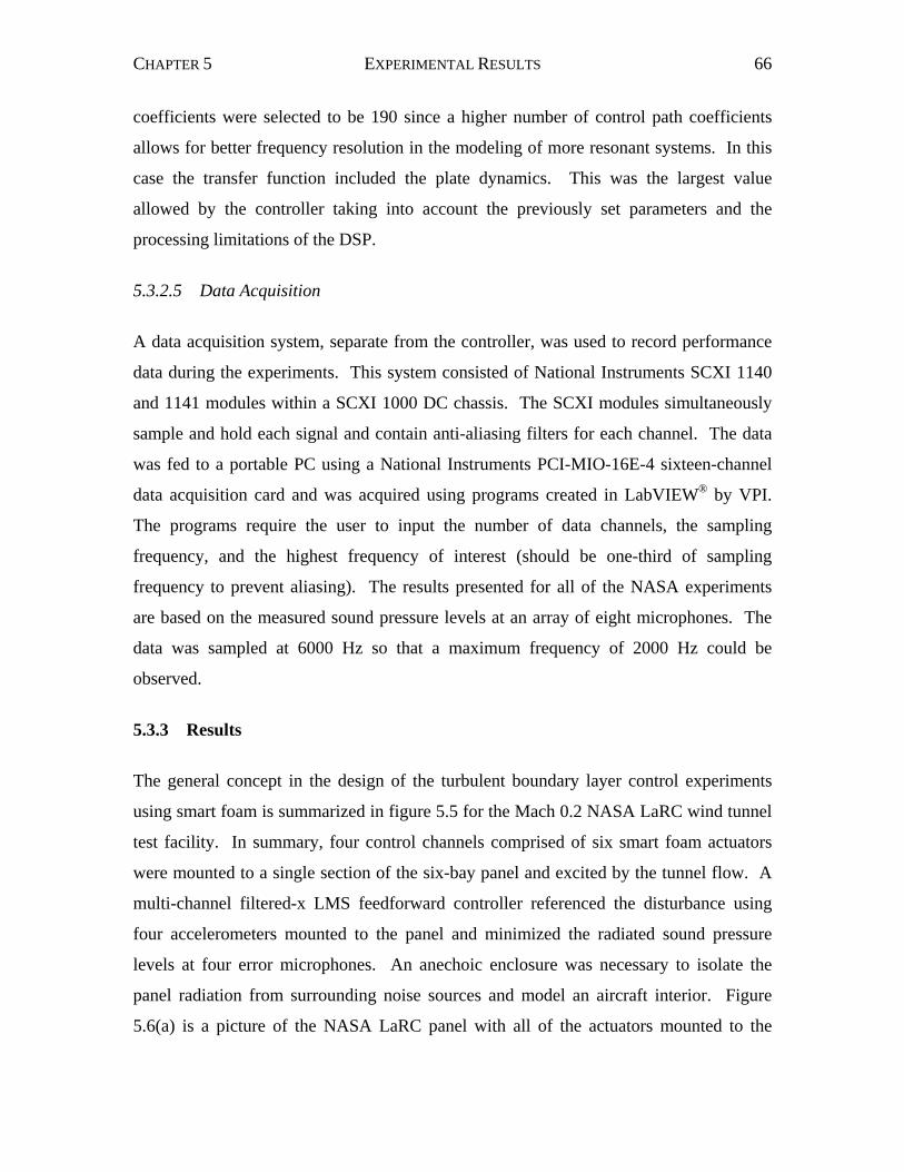
CHAPTER 5 EXPERIMENTAL RESULTS 66
coefficients were selected to be 190 since a higher number of control path coefficients
allows for better frequency resolution in the modeling of more resonant systems. In this
case the transfer function included the plate dynamics. This was the largest value
allowed by the controller taking into account the previously set parameters and the
processing limitations of the DSP.
5.3.2.5 Data Acquisition
A data acquisition system, separate from the controller, was used to record performance
data during the experiments. This system consisted of National Instruments SCXI 1140
and 1141 modules within a SCXI 1000 DC chassis. The SCXI modules simultaneously
sample and hold each signal and contain anti-aliasing filters for each channel. The data
was fed to a portable PC using a National Instruments PCI-MIO-16E-4 sixteen-channel
data acquisition card and was acquired using programs created in LabVIEW® by VPI.
The programs require the user to input the number of data channels, the sampling
frequency, and the highest frequency of interest (should be one-third of sampling
frequency to prevent aliasing). The results presented for all of the NASA experiments
are based on the measured sound pressure levels at an array of eight microphones. The
data was sampled at 6000 Hz so that a maximum frequency of 2000 Hz could be
observed.
5.3.3 Results
The general concept in the design of the turbulent boundary layer control experiments
using smart foam is summarized in figure 5.5 for the Mach 0.2 NASA LaRC wind tunnel
test facility. In summary, four control channels comprised of six smart foam actuators
were mounted to a single section of the six-bay panel and excited by the tunnel flow. A
multi-channel filtered-x LMS feedforward controller referenced the disturbance using
four accelerometers mounted to the panel and minimized the radiated sound pressure
levels at four error microphones. An anechoic enclosure was necessary to isolate the
panel radiation from surrounding noise sources and model an aircraft interior. Figure
5.6(a) is a picture of the NASA LaRC panel with all of the actuators mounted to the
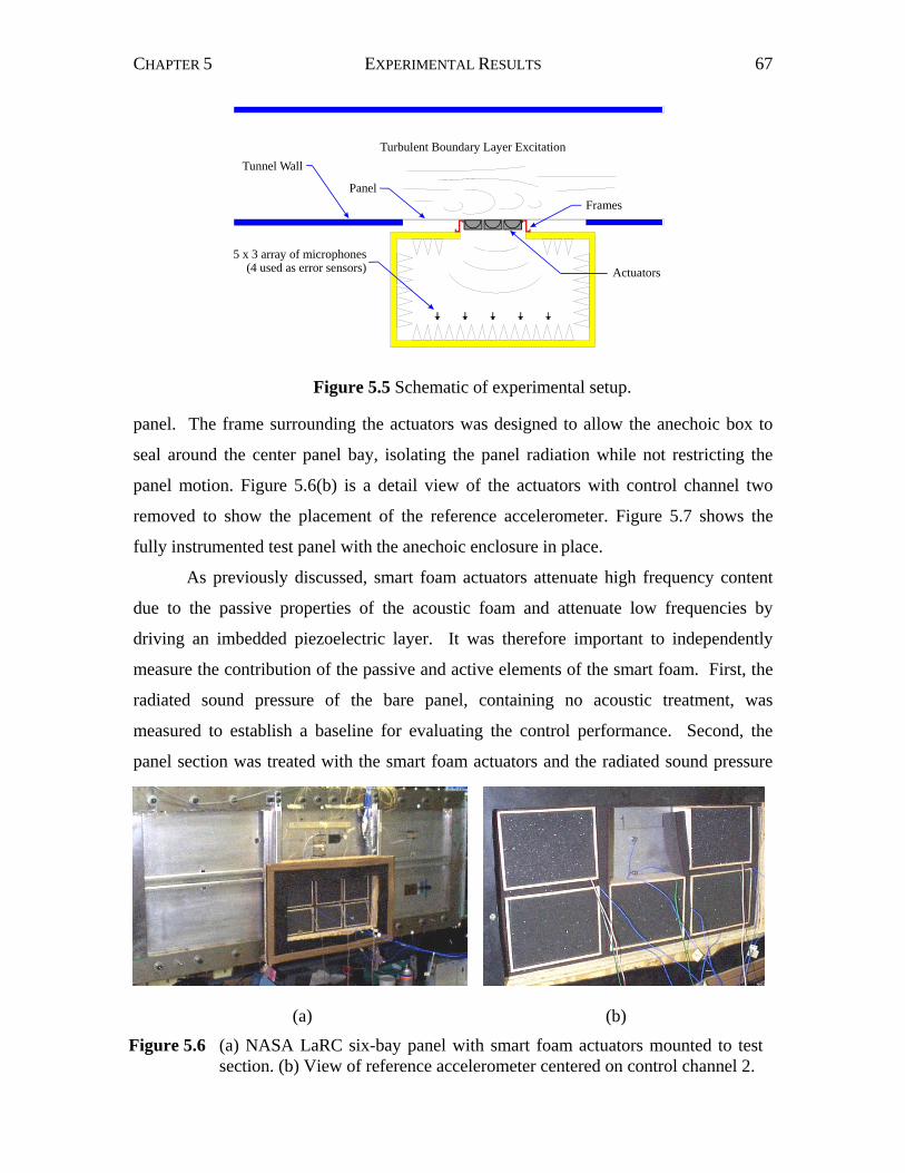
CHAPTER 5 EXPERIMENTAL RESULTS 67
panel. The frame surrounding the actuators was designed to allow the anechoic box to
seal around the center panel bay, isolating the panel radiation while not restricting the
panel motion. Figure 5.6(b) is a detail view of the actuators with control channel two
removed to show the placement of the reference accelerometer. Figure 5.7 shows the
fully instrumented test panel with the anechoic enclosure in place.
As previously discussed, smart foam actuators attenuate high frequency content
due to the passive properties of the acoustic foam and attenuate low frequencies by
driving an imbedded piezoelectric layer. It was therefore important to independently
measure the contribution of the passive and active elements of the smart foam. First, the
radiated sound pressure of the bare panel, containing no acoustic treatment, was
measured to establish a baseline for evaluating the control performance. Second, the
panel section was treated with the smart foam actuators and the radiated sound pressure
(a) (b)
Figure 5.6 (a) NASA LaRC six-bay panel with smart foam actuators mounted to test section. (b) View of reference accelerometer centered on control channel 2.
Figure 5.5 Schematic of experimental setup.
5 x 3 array of microphones(4 used as error sensors)
Turbulent Boundary Layer Excitation
Frames
Actuators
Panel
Tunnel Wall
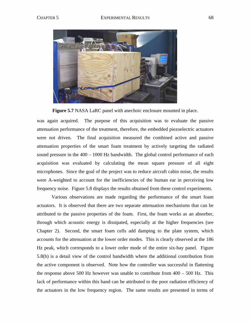
CHAPTER 5 EXPERIMENTAL RESULTS 68
was again acquired. The purpose of this acquisition was to evaluate the passive
attenuation performance of the treatment, therefore, the embedded piezoelectric actuators
were not driven. The final acquisition measured the combined active and passive
attenuation properties of the smart foam treatment by actively targeting the radiated
sound pressure in the 400 – 1000 Hz bandwidth. The global control performance of each
acquisition was evaluated by calculating the mean square pressure of all eight
microphones. Since the goal of the project was to reduce aircraft cabin noise, the results
were A-weighted to account for the inefficiencies of the human ear in perceiving low
frequency noise. Figure 5.8 displays the results obtained from these control experiments.
Various observations are made regarding the performance of the smart foam
actuators. It is observed that there are two separate attenuation mechanisms that can be
attributed to the passive properties of the foam. First, the foam works as an absorber,
through which acoustic energy is dissipated, especially at the higher frequencies (see
Chapter 2). Second, the smart foam cells add damping to the plate system, which
accounts for the attenuation at the lower order modes. This is clearly observed at the 186
Hz peak, which corresponds to a lower order mode of the entire six-bay panel. Figure
5.8(b) is a detail view of the control bandwidth where the additional contribution from
the active component is observed. Note how the controller was successful in flattening
the response above 500 Hz however was unable to contribute from 400 – 500 Hz. This
lack of performance within this band can be attributed to the poor radiation efficiency of
the actuators in the low frequency region. The same results are presented in terms of
Figure 5.7 NASA LaRC panel with anechoic enclosure mounted in place.
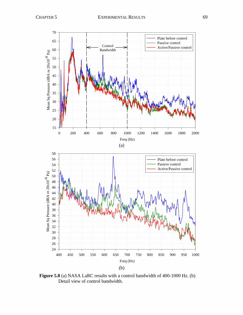
CHAPTER 5 EXPERIMENTAL RESULTS 69
Freq (Hz)
0 200 400 600 800 1000 1200 1400 1600 1800 2000
Mea
n Sq
Pre
ssur
e (d
BA
re 2
0x10
-6 P
a)
15
20
25
30
35
40
45
50
55
60
65
70Plate before controlPassive controlActive/Passive controlControl
Bandwidth
(a)
Freq (Hz)
400 450 500 550 600 650 700 750 800 850 900 950 1000
Mea
n Sq
Pre
ssur
e (d
BA
re 2
0x10
-6 P
a)
242628303234363840424446485052545658
Plate before controlPassive controlActive/Passive control
(b)
Figure 5.8 (a) NASA LaRC results with a control bandwidth of 400-1000 Hz. (b) Detail view of control bandwidth.
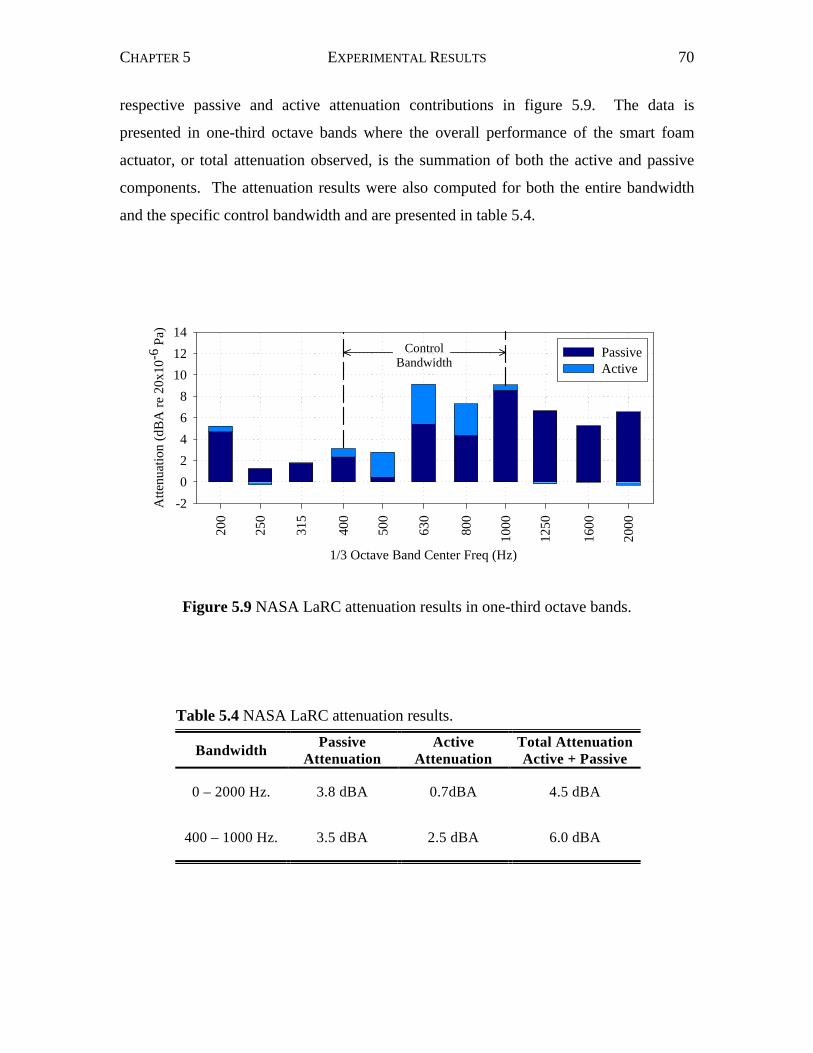
CHAPTER 5 EXPERIMENTAL RESULTS 70
respective passive and active attenuation contributions in figure 5.9. The data is
presented in one-third octave bands where the overall performance of the smart foam
actuator, or total attenuation observed, is the summation of both the active and passive
components. The attenuation results were also computed for both the entire bandwidth
and the specific control bandwidth and are presented in table 5.4.
1/3 Octave Band Center Freq (Hz)
200
250
315
400
500
630
800
1000
1250
1600
2000
Atte
nuat
ion
(dB
A re
20x
10-6
Pa)
-202468
101214
PassiveActive
ControlBandwidth
Bandwidth PassiveAttenuation
ActiveAttenuation
Total AttenuationActive + Passive
0 – 2000 Hz. 3.8 dBA 0.7dBA 4.5 dBA
400 – 1000 Hz. 3.5 dBA 2.5 dBA 6.0 dBA
Figure 5.9 NASA LaRC attenuation results in one-third octave bands.
Table 5.4 NASA LaRC attenuation results.
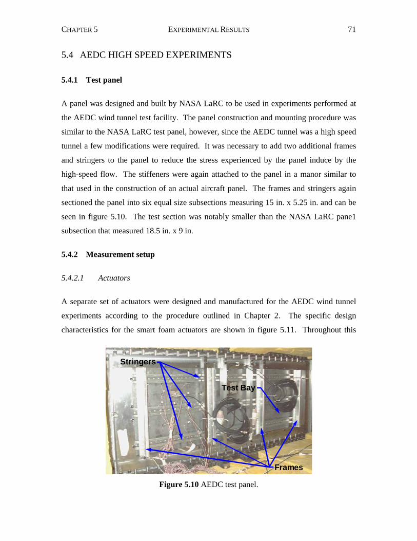
CHAPTER 5 EXPERIMENTAL RESULTS 71
5.4 AEDC HIGH SPEED EXPERIMENTS 5.4.1 Test panel
A panel was designed and built by NASA LaRC to be used in experiments performed at
the AEDC wind tunnel test facility. The panel construction and mounting procedure was
similar to the NASA LaRC test panel, however, since the AEDC tunnel was a high speed
tunnel a few modifications were required. It was necessary to add two additional frames
and stringers to the panel to reduce the stress experienced by the panel induce by the
high-speed flow. The stiffeners were again attached to the panel in a manor similar to
that used in the construction of an actual aircraft panel. The frames and stringers again
sectioned the panel into six equal size subsections measuring 15 in. x 5.25 in. and can be
seen in figure 5.10. The test section was notably smaller than the NASA LaRC pane1
subsection that measured 18.5 in. x 9 in.
5.4.2 Measurement setup
5.4.2.1 Actuators
A separate set of actuators were designed and manufactured for the AEDC wind tunnel
experiments according to the procedure outlined in Chapter 2. The specific design
characteristics for the smart foam actuators are shown in figure 5.11. Throughout this
Stringers
Frames
Test Bay
Figure 5.10 AEDC test panel.
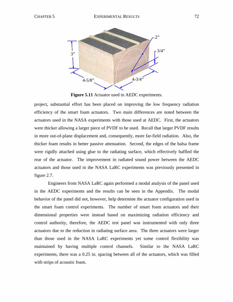
CHAPTER 5 EXPERIMENTAL RESULTS 72
project, substantial effort has been placed on improving the low frequency radiation
efficiency of the smart foam actuators. Two main differences are noted between the
actuators used in the NASA experiments with those used at AEDC. First, the actuators
were thicker allowing a larger piece of PVDF to be used. Recall that larger PVDF results
in more out-of-plane displacement and, consequently, more far-field radiation. Also, the
thicker foam results in better passive attenuation. Second, the edges of the balsa frame
were rigidly attached using glue to the radiating surface, which effectively baffled the
rear of the actuator. The improvement in radiated sound power between the AEDC
actuators and those used in the NASA LaRC experiments was previously presented in
figure 2.7.
Engineers from NASA LaRC again performed a modal analysis of the panel used
in the AEDC experiments and the results can be seen in the Appendix. The modal
behavior of the panel did not, however, help determine the actuator configuration used in
the smart foam control experiments. The number of smart foam actuators and their
dimensional properties were instead based on maximizing radiation efficiency and
control authority, therefore, the AEDC test panel was instrumented with only three
actuators due to the reduction in radiating surface area. The three actuators were larger
than those used in the NASA LaRC experiments yet some control flexibility was
maintained by having multiple control channels. Similar to the NASA LaRC
experiments, there was a 0.25 in. spacing between all of the actuators, which was filled
with strips of acoustic foam.
3”
2”
4-3/4”4-5/8”
3/4”
Figure 5.11 Actuator used in AEDC experiments.
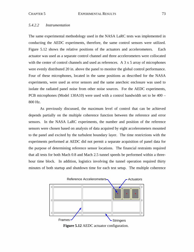
CHAPTER 5 EXPERIMENTAL RESULTS 73
5.4.2.2 Instrumentation
The same experimental methodology used in the NASA LaRC tests was implemented in
conducting the AEDC experiments, therefore, the same control sensors were utilized.
Figure 5.12 shows the relative positions of the actuators and accelerometers. Each
actuator was used as a separate control channel and three accelerometers were collocated
with the center of control channels and used as references. A 3 x 5 array of microphones
were evenly distributed 20 in. above the panel to monitor the global control performance.
Four of these microphones, located in the same positions as described for the NASA
experiments, were used as error sensors and the same anechoic enclosure was used to
isolate the radiated panel noise from other noise sources. For the AEDC experiments,
PCB microphones (Model 130A10) were used with a control bandwidth set to be 400 –
800 Hz.
As previously discussed, the maximum level of control that can be achieved
depends partially on the multiple coherence function between the reference and error
sensors. In the NASA LaRC experiments, the number and position of the reference
sensors were chosen based on analysis of data acquired by eight accelerometers mounted
to the panel and excited by the turbulent boundary layer. The time restrictions with the
experiments performed at AEDC did not permit a separate acquisition of panel data for
the purpose of determining reference sensor locations. The financial restraints required
that all tests for both Mach 0.8 and Mach 2.5 tunnel speeds be performed within a three-
hour time block. In addition, logistics involving the tunnel operation required thirty
minutes of both startup and shutdown time for each test setup. The multiple coherence
Reference Accelerometers Actuators
StringersFrames
Figure 5.12 AEDC actuator configuration.
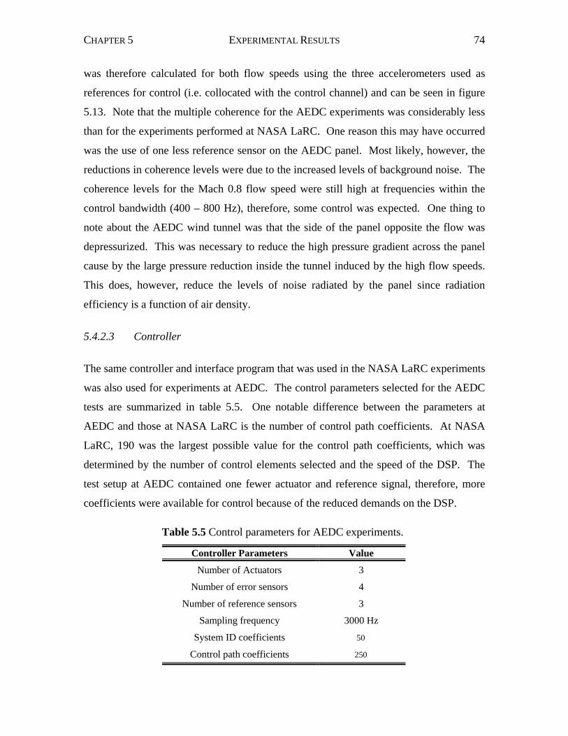
CHAPTER 5 EXPERIMENTAL RESULTS 74
was therefore calculated for both flow speeds using the three accelerometers used as
references for control (i.e. collocated with the control channel) and can be seen in figure
5.13. Note that the multiple coherence for the AEDC experiments was considerably less
than for the experiments performed at NASA LaRC. One reason this may have occurred
was the use of one less reference sensor on the AEDC panel. Most likely, however, the
reductions in coherence levels were due to the increased levels of background noise. The
coherence levels for the Mach 0.8 flow speed were still high at frequencies within the
control bandwidth (400 – 800 Hz), therefore, some control was expected. One thing to
note about the AEDC wind tunnel was that the side of the panel opposite the flow was
depressurized. This was necessary to reduce the high pressure gradient across the panel
cause by the large pressure reduction inside the tunnel induced by the high flow speeds.
This does, however, reduce the levels of noise radiated by the panel since radiation
efficiency is a function of air density.
5.4.2.3 Controller
The same controller and interface program that was used in the NASA LaRC experiments
was also used for experiments at AEDC. The control parameters selected for the AEDC
tests are summarized in table 5.5. One notable difference between the parameters at
AEDC and those at NASA LaRC is the number of control path coefficients. At NASA
LaRC, 190 was the largest possible value for the control path coefficients, which was
determined by the number of control elements selected and the speed of the DSP. The
test setup at AEDC contained one fewer actuator and reference signal, therefore, more
coefficients were available for control because of the reduced demands on the DSP.
Table 5.5 Control parameters for AEDC experiments.
Controller Parameters Value
Number of Actuators 3
Number of error sensors 4
Number of reference sensors 3
Sampling frequency 3000 Hz
System ID coefficients ??
Control path coefficients ???
50
250
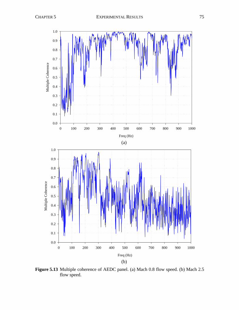
CHAPTER 5 EXPERIMENTAL RESULTS 75
Freq (Hz)
0 100 200 300 400 500 600 700 800 900 1000
Mul
tiple
Coh
eren
ce
0.0
0.1
0.2
0.3
0.4
0.5
0.6
0.7
0.8
0.9
1.0
(a)
Freq (Hz)
0 100 200 300 400 500 600 700 800 900 1000
Mul
tiple
Coh
eren
ce
0.0
0.1
0.2
0.3
0.4
0.5
0.6
0.7
0.8
0.9
1.0
(b)
Figure 5.13 Multiple coherence of AEDC panel. (a) Mach 0.8 flow speed. (b) Mach 2.5 flow speed.
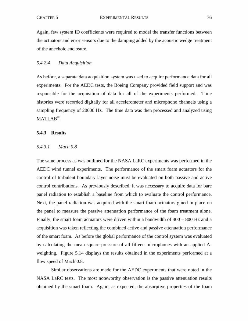
CHAPTER 5 EXPERIMENTAL RESULTS 76
Again, few system ID coefficients were required to model the transfer functions between
the actuators and error sensors due to the damping added by the acoustic wedge treatment
of the anechoic enclosure.
5.4.2.4 Data Acquisition
As before, a separate data acquisition system was used to acquire performance data for all
experiments. For the AEDC tests, the Boeing Company provided field support and was
responsible for the acquisition of data for all of the experiments performed. Time
histories were recorded digitally for all accelerometer and microphone channels using a
sampling frequency of 20000 Hz. The time data was then processed and analyzed using
MATLAB®.
5.4.3 Results
5.4.3.1 Mach 0.8
The same process as was outlined for the NASA LaRC experiments was performed in the
AEDC wind tunnel experiments. The performance of the smart foam actuators for the
control of turbulent boundary layer noise must be evaluated on both passive and active
control contributions. As previously described, it was necessary to acquire data for bare
panel radiation to establish a baseline from which to evaluate the control performance.
Next, the panel radiation was acquired with the smart foam actuators glued in place on
the panel to measure the passive attenuation performance of the foam treatment alone.
Finally, the smart foam actuators were driven within a bandwidth of 400 – 800 Hz and a
acquisition was taken reflecting the combined active and passive attenuation performance
of the smart foam. As before the global performance of the control system was evaluated
by calculating the mean square pressure of all fifteen microphones with an applied A-
weighting. Figure 5.14 displays the results obtained in the experiments performed at a
flow speed of Mach 0.8.
Similar observations are made for the AEDC experiments that were noted in the
NASA LaRC tests. The most noteworthy observation is the passive attenuation results
obtained by the smart foam. Again, as expected, the absorptive properties of the foam
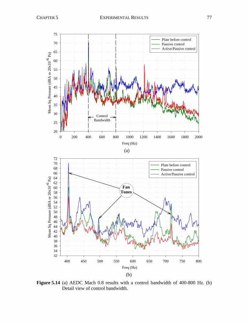
CHAPTER 5 EXPERIMENTAL RESULTS 77
Freq (Hz)
0 200 400 600 800 1000 1200 1400 1600 1800 2000
Mea
n Sq
Pre
ssur
e (d
BA
re 2
0x10
-6 P
a)
20
25
30
35
40
45
50
55
60
65
70
75Plate before control Passive controlActive/Passive control
ControlBandwidth
(a)
Freq (Hz)
400 450 500 550 600 650 700 750 800
Mea
n Sq
Pre
ssur
e (d
BA
re 2
0x10
-6 P
a)
323436384042444648505254565860626466687072
Plate before controlPassive controlActive/Passive control
FanTones
(b)
Figure 5.14 (a) AEDC Mach 0.8 results with a control bandwidth of 400-800 Hz. (b) Detail view of control bandwidth.
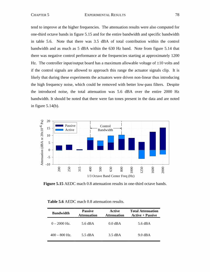
CHAPTER 5 EXPERIMENTAL RESULTS 78
tend to improve at the higher frequencies. The attenuation results were also computed for
one-third octave bands in figure 5.15 and for the entire bandwidth and specific bandwidth
in table 5.6. Note that there was 3.5 dBA of total contribution within the control
bandwidth and as much as 5 dBA within the 630 Hz band. Note from figure 5.14 that
there was negative control performance at the frequencies starting at approximately 1200
Hz. The controller input/output board has a maximum allowable voltage of ±10 volts and
if the control signals are allowed to approach this range the actuator signals clip. It is
likely that during these experiments the actuators were driven non-linear thus introducing
the high frequency noise, which could be removed with better low-pass filters. Despite
the introduced noise, the total attenuation was 5.6 dBA over the entire 2000 Hz
bandwidth. It should be noted that there were fan tones present in the data and are noted
in figure 5.14(b).
Bandwidth PassiveAttenuation
ActiveAttenuation
Total AttenuationActive + Passive
0 – 2000 Hz. 5.6 dBA 0.0 dBA 5.6 dBA
400 – 800 Hz. 5.5 dBA 3.5 dBA 9.0 dBA
Figure 5.15 AEDC mach 0.8 attenuation results in one-third octave bands.
1/3 Octave Band Center Freq (Hz)
200
250
315
400
500
630
800
1000
1250
1600
2000
Atte
nuat
ion
(dB
A re
20x
10-6
Pa)
-10
-5
0
5
10
15
20PassiveActive
ControlBandwidth
Table 5.6 AEDC mach 0.8 attenuation results.
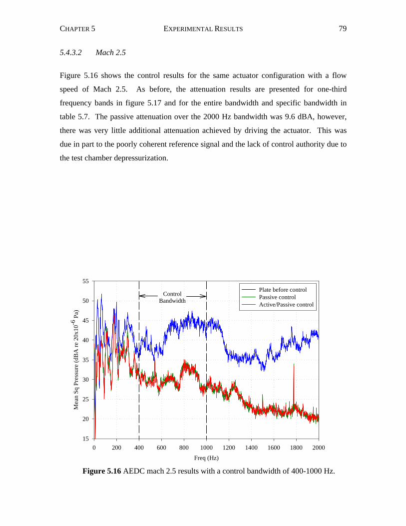
CHAPTER 5 EXPERIMENTAL RESULTS 79
5.4.3.2 Mach 2.5
Figure 5.16 shows the control results for the same actuator configuration with a flow
speed of Mach 2.5. As before, the attenuation results are presented for one-third
frequency bands in figure 5.17 and for the entire bandwidth and specific bandwidth in
table 5.7. The passive attenuation over the 2000 Hz bandwidth was 9.6 dBA, however,
there was very little additional attenuation achieved by driving the actuator. This was
due in part to the poorly coherent reference signal and the lack of control authority due to
the test chamber depressurization.
Freq (Hz)
0 200 400 600 800 1000 1200 1400 1600 1800 2000
Mea
n Sq
Pre
ssur
e (d
BA
re 2
0x10
-6 P
a)
15
20
25
30
35
40
45
50
55Plate before controlPassive controlActive/Passive control
ControlBandwidth
Figure 5.16 AEDC mach 2.5 results with a control bandwidth of 400-1000 Hz.
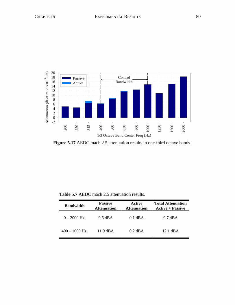
CHAPTER 5 EXPERIMENTAL RESULTS 80
1/3 Octave Band Center Freq (Hz)
200
250
315
400
500
630
800
1000
1250
1600
2000
Atte
nuat
ion
(dB
A re
20x
10-6
Pa)
-202468
101214161820
PassiveActive
ControlBandwidth
Bandwidth PassiveAttenuation
ActiveAttenuation
Total AttenuationActive + Passive
0 – 2000 Hz. 9.6 dBA 0.1 dBA 9.7 dBA
400 – 1000 Hz. 11.9 dBA 0.2 dBA 12.1 dBA
Figure 5.17 AEDC mach 2.5 attenuation results in one-third octave bands.
Table 5.7 AEDC mach 2.5 attenuation results.
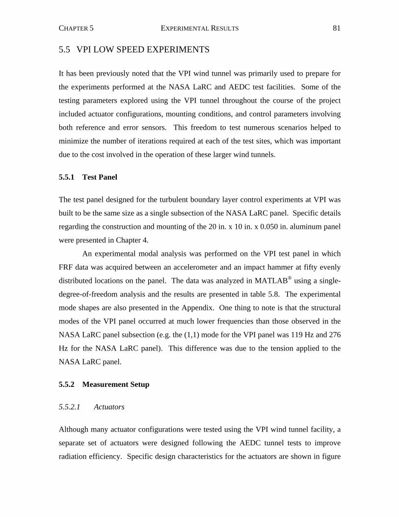
CHAPTER 5 EXPERIMENTAL RESULTS 81
5.5 VPI LOW SPEED EXPERIMENTS It has been previously noted that the VPI wind tunnel was primarily used to prepare for
the experiments performed at the NASA LaRC and AEDC test facilities. Some of the
testing parameters explored using the VPI tunnel throughout the course of the project
included actuator configurations, mounting conditions, and control parameters involving
both reference and error sensors. This freedom to test numerous scenarios helped to
minimize the number of iterations required at each of the test sites, which was important
due to the cost involved in the operation of these larger wind tunnels.
5.5.1 Test Panel
The test panel designed for the turbulent boundary layer control experiments at VPI was
built to be the same size as a single subsection of the NASA LaRC panel. Specific details
regarding the construction and mounting of the 20 in. x 10 in. x 0.050 in. aluminum panel
were presented in Chapter 4.
An experimental modal analysis was performed on the VPI test panel in which
FRF data was acquired between an accelerometer and an impact hammer at fifty evenly
distributed locations on the panel. The data was analyzed in MATLAB® using a single-
degree-of-freedom analysis and the results are presented in table 5.8. The experimental
mode shapes are also presented in the Appendix. One thing to note is that the structural
modes of the VPI panel occurred at much lower frequencies than those observed in the
NASA LaRC panel subsection (e.g. the (1,1) mode for the VPI panel was 119 Hz and 276
Hz for the NASA LaRC panel). This difference was due to the tension applied to the
NASA LaRC panel.
5.5.2 Measurement Setup
5.5.2.1 Actuators
Although many actuator configurations were tested using the VPI wind tunnel facility, a
separate set of actuators were designed following the AEDC tunnel tests to improve
radiation efficiency. Specific design characteristics for the actuators are shown in figure
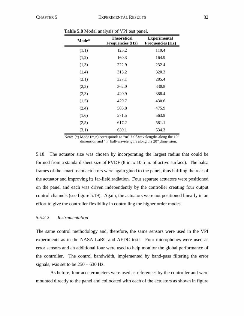
CHAPTER 5 EXPERIMENTAL RESULTS 82
5.18. The actuator size was chosen by incorporating the largest radius that could be
formed from a standard sheet size of PVDF (8 in. x 10.5 in. of active surface). The balsa
frames of the smart foam actuators were again glued to the panel, thus baffling the rear of
the actuator and improving its far-field radiation. Four separate actuators were positioned
on the panel and each was driven independently by the controller creating four output
control channels (see figure 5.19). Again, the actuators were not positioned linearly in an
effort to give the controller flexibility in controlling the higher order modes.
5.5.2.2 Instrumentation
The same control methodology and, therefore, the same sensors were used in the VPI
experiments as in the NASA LaRC and AEDC tests. Four microphones were used as
error sensors and an additional four were used to help monitor the global performance of
the controller. The control bandwidth, implemented by band-pass filtering the error
signals, was set to be 250 – 630 Hz.
As before, four accelerometers were used as references by the controller and were
mounted directly to the panel and collocated with each of the actuators as shown in figure
Mode* TheoreticalFrequencies (Hz)
ExperimentalFrequencies (Hz)
(1,1) 125.2 119.4
(1,2) 160.3 164.9
(1,3) 222.9 232.4
(1,4) 313.2 320.3
(2.1) 327.1 285.4
(2,2) 362.0 330.8
(2,3) 420.9 388.4
(1,5) 429.7 430.6
(2,4) 505.8 475.9
(1,6) 571.5 563.8
(2,5) 617.2 581.1
(3,1) 630.1 534.3Note: (*) Mode (m,n) corresponds to “m” half-wavelengths along the 10”
dimension and “n” half-wavelengths along the 20” dimension.
Table 5.8 Modal analysis of VPI test panel.
CHAPTER 5 EXPERIMENTAL RESULTS 83
5.19. The multiple coherence was also measured to establish whether the chosen
accelerometer locations provided a coherent signal with each of the actuators. The
multiple coherence measured at one of the microphones is shown in figure 5.20.
5.5.2.3 Control and Data Acquisition
The experiments performed at VPI contained the same number of actuator, error, and
reference channels as the NASA LaRC experiments, therefore, the parameters selected
for control were the same as were summarized in table 5.3. Likewise, the same data
acquisition equipment and programs were used to collect and record the data, which was
again was sampled at 6000 Hz.
ReferenceAccelerometers
Figure 5.18 Actuator used in VPI experiments.
3-1/2”
3-1/4”
7-1/4”
3-1/4”
Figure 5.19 VPI actuator configuration.
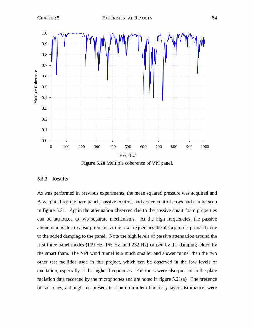
CHAPTER 5 EXPERIMENTAL RESULTS 84
5.5.3 Results
As was performed in previous experiments, the mean squared pressure was acquired and
A-weighted for the bare panel, passive control, and active control cases and can be seen
in figure 5.21. Again the attenuation observed due to the passive smart foam properties
can be attributed to two separate mechanisms. At the high frequencies, the passive
attenuation is due to absorption and at the low frequencies the absorption is primarily due
to the added damping to the panel. Note the high levels of passive attenuation around the
first three panel modes (119 Hz, 165 Hz, and 232 Hz) caused by the damping added by
the smart foam. The VPI wind tunnel is a much smaller and slower tunnel than the two
other test facilities used in this project, which can be observed in the low levels of
excitation, especially at the higher frequencies. Fan tones were also present in the plate
radiation data recorded by the microphones and are noted in figure 5.21(a). The presence
of fan tones, although not present in a pure turbulent boundary layer disturbance, were
Freq (Hz)
0 100 200 300 400 500 600 700 800 900 1000
Mul
tiple
Coh
eren
ce
0.0
0.1
0.2
0.3
0.4
0.5
0.6
0.7
0.8
0.9
1.0
Figure 5.20 Multiple coherence of VPI panel.
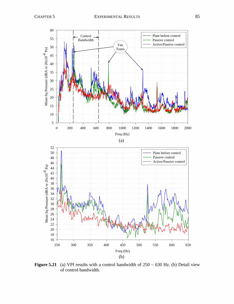
CHAPTER 5 EXPERIMENTAL RESULTS 85
Freq (Hz)
0 200 400 600 800 1000 1200 1400 1600 1800 2000
Mea
n Sq
Pre
ssur
e (d
BA
re 2
0x10
-6 P
a)
5
10
15
20
25
30
35
40
45
50
55
60Plate before controlPassive controlActive/Passive control
ControlBandwidth
FanTones
(a)
Freq (Hz)
250 300 350 400 450 500 550 600 650
Mea
n Sq
Pre
ssur
e (d
BA
re 2
0x10
-6 P
a)
16182022242628303234363840424446485052
Plate before controlPassive controlActive/Passive control
(b)
Figure 5.21 (a) VPI results with a control bandwidth of 250 − 630 Hz. (b) Detail view of control bandwidth.
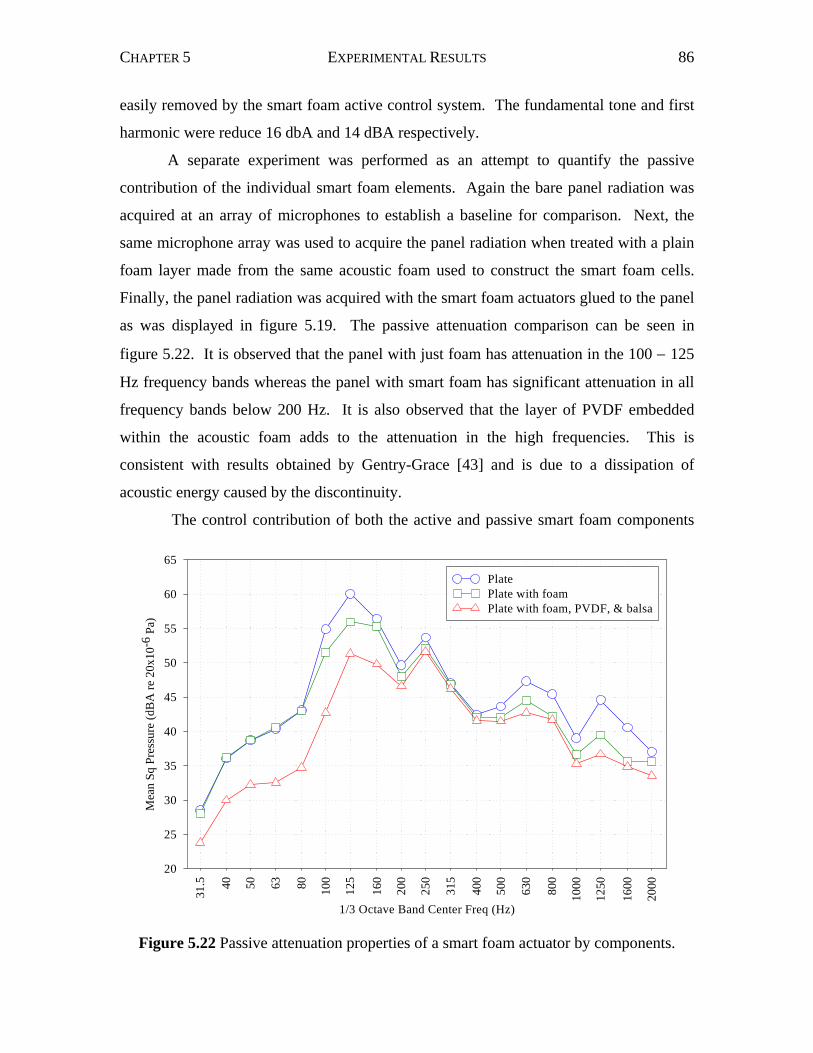
CHAPTER 5 EXPERIMENTAL RESULTS 86
easily removed by the smart foam active control system. The fundamental tone and first
harmonic were reduce 16 dbA and 14 dBA respectively.
A separate experiment was performed as an attempt to quantify the passive
contribution of the individual smart foam elements. Again the bare panel radiation was
acquired at an array of microphones to establish a baseline for comparison. Next, the
same microphone array was used to acquire the panel radiation when treated with a plain
foam layer made from the same acoustic foam used to construct the smart foam cells.
Finally, the panel radiation was acquired with the smart foam actuators glued to the panel
as was displayed in figure 5.19. The passive attenuation comparison can be seen in
figure 5.22. It is observed that the panel with just foam has attenuation in the 100 − 125
Hz frequency bands whereas the panel with smart foam has significant attenuation in all
frequency bands below 200 Hz. It is also observed that the layer of PVDF embedded
within the acoustic foam adds to the attenuation in the high frequencies. This is
consistent with results obtained by Gentry-Grace [43] and is due to a dissipation of
acoustic energy caused by the discontinuity.
The control contribution of both the active and passive smart foam components
1/3 Octave Band Center Freq (Hz)
31.5 40 50 63 80 100
125
160
200
250
315
400
500
630
800
1000
1250
1600
2000
Mea
n Sq
Pre
ssur
e (d
BA
re 2
0x10
-6 P
a)
20
25
30
35
40
45
50
55
60
65PlatePlate with foamPlate with foam, PVDF, & balsa
Figure 5.22 Passive attenuation properties of a smart foam actuator by components.
CHAPTER 5 EXPERIMENTAL RESULTS 87
can be seen in figure 5.23. The active elements of the smart foam actuators were able to
significant contribute to the attenuation across the entire control bandwidth between 250
– 630 Hz. The control achieved in the 200 Hz and 800 Hz frequency bands was due to
roll-off in the filters used to band-pass filter the error signals prior to entering the
controller. Notice that in the 1000 Hz, 1250Hz, and 1600 Hz octave bands, the active
control signals slightly increased the sound pressure levels. As the filtered-x LMS
control algorithm tries to minimize (or flatten) the response at the error microphones,
frequencies that are less dominant in the overall pressure spectrum are raised in an effort
to control the most dominant frequencies. The attenuation results are tabulated for the
entire bandwidth and the specific control bandwidths in table 5.9. The active attenuation
contribution over the entire frequency spectrum has been improved to 1.6 dBA whereas
in the NASA LaRC tests only 0.7 dbA was realized. This can be attributed to the
improved control authority at low frequencies accomplished by increasing the physical
size of the active layer and by gluing the balsa to the radiating structure. The
improvements allowed the active control bandwidth for the VPI experiments to start at
250 Hz whereas the NASA LaRC control bandwidth started at 500 Hz. Although the
AEDC actuators were glued to the structure, the bandwidth was unable to be set below
400 Hz because of the loss of control authority due to the depressurized test chamber.
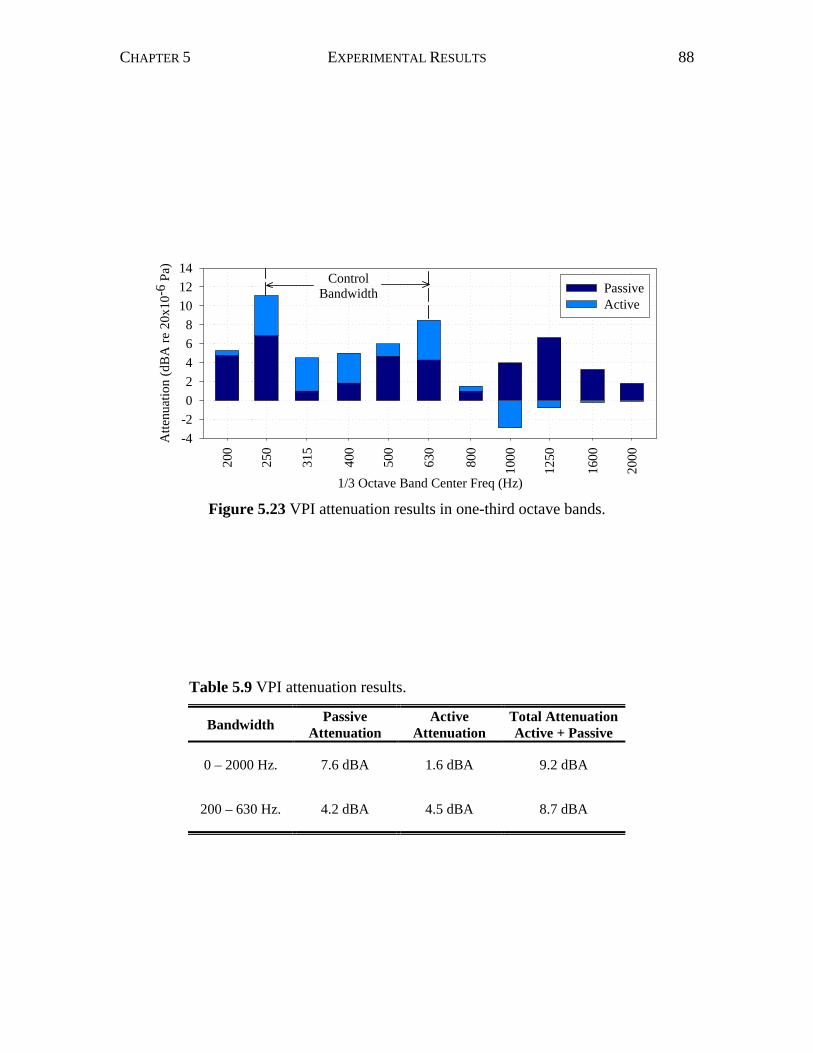
CHAPTER 5 EXPERIMENTAL RESULTS 88
1/3 Octave Band Center Freq (Hz)
200
250
315
400
500
630
800
1000
1250
1600
2000
Atte
nuat
ion
(dB
A re
20x
10-6
Pa)
-4-202468
101214
PassiveActive
ControlBandwidth
Figure 5.23 VPI attenuation results in one-third octave bands.
Table 5.9 VPI attenuation results.
Bandwidth PassiveAttenuation
ActiveAttenuation
Total AttenuationActive + Passive
0 – 2000 Hz. 7.6 dBA 1.6 dBA 9.2 dBA
200 – 630 Hz. 4.2 dBA 4.5 dBA 8.7 dBA
89
Chapter 6 Conclusions and Future Work The effectiveness of smart foam actuators in controlling panel sound radiation excited by
a turbulent boundary layer disturbance has been demonstrated. Smart foam is a hybrid
device combining acoustic foam and an embedded PVDF smart skin. The foam works as
an acoustic absorber that attenuates the high-frequency content, while the PVDF is driven
actively and used to overcome the limitations of the foam at low frequencies. The smart
foam actuator is therefore an effective control device for broadband applications and, due
to its lightweight when compared to conventional speakers, is an ideal control device for
aircraft noise problems.
An experimental methodology was developed for testing the control of aircraft
panel radiation using smart foam actuators and was tested using three separate wind
tunnel testing facilities. A test panel, representing the exterior fuselage skin of an
aircraft, was mounted on the wall of a wind tunnel. The tunnel flow was then used to
excite the panel that, consequently, radiated sound into an anechoic enclosure
representative of an aircraft cabin. Within the anechoic enclosure was a series of smart
foam actuators mounted to the panel and an array of microphones used to monitor the
performance of the control system. A multiple channel feedforward filtered-x LMS
control algorithm was used to drive the smart foam actuators such that the superposition
of the actuator generated sound and the panel noise produced cancellation at the error
microphones.
One characteristic of a smart foam actuator is the poor radiation efficiency of the
device at low frequencies (i.e. <250 Hz). Most piezoelectric materials, including PVDF,
CHAPTER 6 CONCLUSIONS AND FUTURE WORK 90
do not generate large displacements for an applied voltage, which is a fundamental
requirement in the generation of low-frequency noise. The PVDF is positioned within
the acoustic foam in a half-cylinder configuration to couple the in-plane strain associated
with the piezoelectric effect with a maximum amount of vertical displacement. The smart
foam cell is then housed within a balsa frame that both anchors the ends of the PVDF and
serves as a baffle. Effort throughout the project was focused on improving the
performance of the smart foam actuators at low frequencies.
Successful broadband control results were achieved using two separate low-speed
wind tunnel test facilities. The smart foam actuators were tested on a Mach 0.2 wind
tunnel at the NASA Langley Research Center (NASA LaRC). Across the 0 – 2000 Hz
frequency band a total attenuation of 4.5 dBA was achieved where 3.8 dBA was due to
the passive contribution. The active control element was driven in the 400 – 1000 Hz
where attenuation of 2.5 dBA was realized. A similar set of experiments were later
performed on a Mach 0.1 wind tunnel belonging to Virginia Polytechnic Institute and
State University (VPI). Two key modifications were made to the actuators prior to the
testing at VPI. The first modification was that the actuators were physically larger in size
in order to incorporate a larger piece of PVDF. The second modification included gluing
the edges of the balsa frame to the radiating panel thus baffling the backside of the
actuator and improving its radiation efficiency. Experiments were performed and from 0
– 2000 Hz attenuation of 9.2 dBA was obtained with 7.6 dBA contributed passively.
Actively the smart foam was able to contribute 4.5 dBA between 250 – 630 Hz. The
increase in performance can be attributed to the improvements in control authority at low
frequencies due to the smart foam modifications.
Broadband control results were also achieved using the high-speed wind tunnel
test facility at the Arnold Engineering Development Center (AEDC). At the Mach 0.8
flow speed, 5.6 dBA of total attenuation was obtained all coming from the passive
properties of the foam. Active contribution was 3.5 dBA in the 400 – 800 Hz bandwidth.
At the Mach 2.5 flow speed, a total attenuation of 9.7 dBA was achieved with 9.6 dBA
coming from the passive properties of the smart foam. Although the smart foam
actuators were large and the frame was glued to the panel, control authority was
compromised in the high-speed experiments because the test chamber was depressurized.
CHAPTER 6 CONCLUSIONS AND FUTURE WORK 91
The potential for smart foam in controlling broadband radiation due to a turbulent
boundary layer disturbance has been demonstrated for various flight conditions. It is
clear from these experiments that future improvements in results depend on the ability to
increase control authority at low frequencies. The smart foam actuators used in the VPI
experiments were able exhibit control as low as 250 Hz octave band, however, a
disturbance with dominant noise contribution below this frequency could not be
controlled with the current smart foam actuator configuration.
Future work with smart foam could include the use of near-field microphones as
error sensors. This change allows the multiple control channels to become decoupled and
closer approximates the necessary requirements for implementation into an actual
aircraft. Some preliminary experiments have been performed with near-field error
microphones and show promising results. Also, a more detailed study into understanding
and improving the passive properties of each individual component of the smart foam
actuator could be performed. A current modification to the smart foam actuator that is
being considered is the addition of a distributed mass layer. This mass layer could be
tuned to a frequency below the operating range of the smart foam active layer and work
as tuned vibration absorber. Due to the inherent flexibility of the smart foam components
and their construction, there exists great potential for incorporating additional noise
control strategies into the already robust smart foam actuator.
92
Bibliography [1] W.L. Willshire, Jr. and D.G. Stephens, “Aircraft noise technology for the 21st
century,” Proceedings of Noise-Con 98, pp. 7-22, 1998.
[2] J.F. Wilby, “Aircraft interior noise,” Journal Of Sound and Vibration, 190(3), pp.
545-564, 1996.
[3] D.E. Bishop, “Cruise flight noise levels in a turbojet transport airplane,” Noise
Control 7, pp. 37-42, 1961.
[4] N.J. Fleming, “The silencing of aircraft,” Journal of the Royal Aeronautical
Society, 50, pp. 639-676, 1946.
[5] R.E. Hayden, B.S. Murray, and M.A. Theobald, “Boundary-layer-induced noise
in the interior of aircraft, “ NASA CR-172152, 1983.
[6] D.A. Bies, “A review of flight and wind tunnel measurements of boundary layer
pressure fluctuations and induced structural response,” NASA CR-626, 1966.
[7] W.V Bhat, “Flight test measurement of exterior turbulent boundary layer pressure
fluctuations on Boeing model 737 airplane,” Journal of Sound and Vibration, 14,
pp. 439-457, 1971.
[8] W.V. Bhat and J.F. Wilby, “Interior noise radiated by an airplane fuselage
subjected to turbulent boundary layer excitation and evaluation of noise reduction
treatments,” Journal of Sound and Vibration, 17, pp. 449-464, 1971.
[9] L. Maestrello, “Measurement and analysis of the response field of turbulent
boundary layer excited panels,” Journal of Sound and Vibration, 2(3), pp. 270-
292, 1965.
[10] L. Maestrello, “Radiation from and panel response to a supersonic turbulent
boundary layer,” Journal of Sound and Vibration, 10(2), pp. 261-295, 1969.
BIBLIOGRAPHY 93
[11] J.F. Wilby and F.L. Gloyna, “Vibration measurements of an airplane fuselage
structure, I: turbulent boundary layer excitation,” Journal of Sound and Vibration,
23, pp. 443-466, 1972.
[12] P.A. Nelson and S.J. Elliot, Active Control of Sound, Academic Press, Inc., San
Diego, CA, 1992.
[13] J.E. Ffowcs Williams, “Anti-sound,” Proc. R. Soc. Lond., A 395, pp. 63-88, 1984.
[14] C.R Fuller, “Apparatus and method for global noise reduction,” U.S. Patent No.
4,715,599, 1987.
[15] C.R. Fuller, “Active control of sound transmission/radiation from elastic plate by
vibration inputs: I. Analysis,” Journal of Sound and Vibration, 136(1), pp. 1-15,
1990.
[16] R.A. Burdisso and C.R. Fuller, “Theory of feedforward controlled system
eigenproperties,” Journal of Sound and Vibration, 153(3), pp. 437-452, 1992.
[17] R.L. Clark, “Advanced sensing techniques for active structural acoustic control,”
Ph.D. Dissertation, Virginia Polytechnic Institute & State University, Department
of Mechanical Engineering, 1992.
[18] B.T. Wang, R.A. Burdisso, and C.R. Fuller, “Optimal placement of piezoelectric
actuators for active control of sound radiation from elastic plates,” Proceedings of
Noise-Con 91, pp. 267-275, 1991.
[19] Clark, R.L., and Fuller, C.R., “Optimal placement of piezoelectric actuators and
polyvinylidene fluoride (PVDF) error sensors in active structural acoustic control
approaches,” Journal of the Acoustical Society of America, 92(3), pp. 1489-1498,
1992.
[20] W.T. Baumann, F. Ho, and H.H. Robertshaw, “Active structural acoustic control
of broadband disturbances,” Journal of the Acoustical Society of America, 92(4),
pp. 1998-2005, 1992.
[21] H.H. Bruderlin, “Developments in aircraft sound control,” Journal of the
Acoustical Society of America, 8, pp. 181-184, 1937.
[22] R.H. Nichols, H.P. Sleeper Jr., R.L. Wallace Jr., and H.L. Ericson, “Acoustical
materials and acoustical treatments for aircraft,” Journal of the Acoustical Society
of America, 19(3), pp. 428-443, 1947.
BIBLIOGRAPHY 94
[23] J.S. Mixson and C.A. Powell, “Review of recent research on interior noise of
propeller driven aircraft,” Journal of Aircraft, 22, pp. 931-949, 1985.
[24] R. Vaicaitis and J.S. Mixson, “Review of research on structureborne noise,” AIAA
Paper, 85-0786, 1985.
[25] M.A. Simpson, T.M. Luong, C.R. Fuller, and J.D. Jones, “Full-scale
demonstration tests of cabin noise reduction using active vibration control,”
Journal of Aircraft, 28(3), pp. 208-215, 1991.
[26] C.R. Fuller and G.P. Gibbs, “Active control of interior noise in a business jet
using piezoceramic actuators,” Noise-Con 94, pp. 389-394, 1994.
[27] S.J. Elliott, P.A. Nelson, I.M. Stothers, and C.C. Boucher, “In-flight experiments
on the active control of propeller-induced cabin noise,” Jounal of Sound and
Vibration, 140(2), pp. 219-238, 1990.
[28] U. Emborg, “Application of active noise control in Saab 340 and Saab 2000,”
Proceedings of the Nordic Conference on Vehicle and Machinery Vibrations,
Stockholm, Sweden, September, 1994.
[29] F.W. Grosveld, “Plate acceleration and sound transmission due to random
acoustic and boundary-layer excitation,” AIAA Journal, Vol. 30, No. 3, pp. 601-
607, 1992.
[30] W.R. Graham, “Boundary layer induced noise in aircraft, Part I: The flat plate
model,” Journal of Sound and Vibration, 192(1), pp. 101-120, 1996.
[31] W.R. Graham, “Boundary layer induced noise in aircraft, Part II: The trimmed flat
plate model,” Journal of Sound and Vibration, 192(1), pp. 121-138, 1996.
[32] B. W. Mahnken, “Active control of aircraft interior flow noise via the use of
active trim panels,” Master’s Thesis, Virginia Polytechnic Institute & State
University, Mechanical Engineering Department, 1996.
[33] L. Beranek and L. Ver, Noise and Vibration Control Engineering: Principles and
Applications, John Wiley & Sons, Inc., New York, NY, 1992.
[34] Y.J. Kang, W. Tsoi, and J.S. Bolton, “The effect of mounting on the acoustical
properties of finite-depth polyimide foam layers,” Proceedings of Noise-Con 93,
Williamsburg, Virginia, pp. 285-290, 1993.
BIBLIOGRAPHY 95
[35] J.S. Bolton and E.R. Green, “Smart foams for active absorption of sound,” Second
Conference on Recent Advances in Active Control of Sound and Vibration,
Blacksburg, Virginia, pp. 139-149, 1993.
[36] C.R. Fuller, M.J. Bronzel, C.A. Gentry, and D.E. Wittington, “Control of sound
radiation/reflection with adaptive foams,” Proceedings of Noise-Con 94, Ft.
Lauderdale, Florida, pp. 429-436, 1994.
[37] S.J. Elliott, “A simple two microphone method of measuring absorption
coefficients,” Acoustic Letters, 5(2), pp. 39-44, 1981.
[38] C.A. Gentry, C. Guigou, and C.R. Fuller, “Smart foam for applications in passive-
active noise radiation control,” Journal of the Acoustical Society of America,
101(4), pp. 1771-1778, 1997.
[39] C.A. Gentry, C. Guigou, and C.R. Fuller, “Smart foam for active/passive plate
radiation control,” Journal of the Acoustical Society of America, (to appear).
[40] C. Guigou and C.R. Fuller, “Control of aircraft interior broadband noise with
foam-PVDF smart skin,” Journal of Sound and Vibration, 220(3), pp. 541-557,
1999.
[41] Measurement Specialties Inc., “Piezo Film Sensors Technical Manual”, Published
by Measurement Specialties Inc., Valley Forge, PA, 1998.
[42] Polymer Technology Inc., “Technical Data Sheet: Acoustical Products-An
Overview,” Published by Polymer Technology Inc., Newark, Delaware, 1994.
[43] C.A. Gentry-Grace, “A Study of Smart Foam for Noise Control Applications,”
Ph.D. Dissertation, Virginia Polytechnic Institute & State University, Mechanical
Engineering Department, 1998.
[44] C. Liang and C.A. Rogers, “A fully coupled acoustic analysis of curved PVDF
acoustic actuators for active sound attenuation,” Materials and Devices, pp. 765-
779.
[45] International Organization for Standardization (ISO), “Acoustics-determination of
sound power levels of noise sources-precision methods for anechoic and semi-
anechoic rooms,” #3745-1977 (E)
[46] P. Lueg, “Process of silencing sound oscillations,” U.S. Patent No. 2,043,416,
1936.
BIBLIOGRAPHY 96
[47] B. Widrow and S.D. Stearns, Adaptive Signal Processing, Prentice-Hall, Inc.,
Englewood Cliffs, NJ, 1985.
[48] S.J. Elliott, I.M. Stothers, and P.A. Nelson, “A multiple error LMS algorithm and
its application to the active control of sound and vibration,” IEEE Transactions on
Acoustics, Speech, and Signal Processing, Vol. ASSP-35. No. 10, pp. 1423-1434,
1987.
[49] R.A. Burdisso, J.S. Vipperman, and C.R. Fuller, “Causality analysis of
feedforward-controlled systems with broadband inputs,” Journal of the Acoustical
Society of America, 94(1), pp. 234-242, 1993.
[50] L.L. Beranek, Noise Reduction, McGraw-Hill Book Company Inc., NY, p. 258,
1960.
[51] Illbruck Inc., “Technical Data Sheet: SONEX Acoustic Products,” Illbruck Inc.,
Minneapolis, MN, 1995.
[52] D.A. Bies and C.H. Hansen, Engineering Noise Control: Theory and Practice,
Second Edition, E&FN Spon, London, UK, p. 233, 1996.

97
Appendix Test Panel Mode Shapes Chapter 5 gave a detailed description of each of the three test panels used in the turbulent
boundary layer control experiments for this project. An experimental modal analysis was
also performed for each of the panels in order to assist in the design and placement of the
smart foam actuators. Chapter 5 also presented a list of modes and their corresponding
frequencies for each of the modals performed. The figures in the appendix are the mode
shapes for each of the panels analyzed.
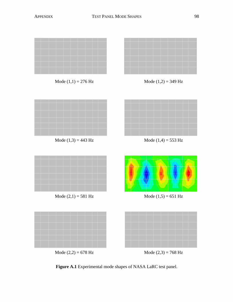
APPENDIX TEST PANEL MODE SHAPES 98
Mode (1,1) = 276 Hz Mode (1,2) = 349 Hz
Mode (1,3) = 443 Hz Mode (1,4) = 553 Hz
Mode (2,1) = 581 Hz Mode (1,5) = 651 Hz
Mode (2,2) = 678 Hz Mode (2,3) = 768 Hz
Figure A.1 Experimental mode shapes of NASA LaRC test panel.
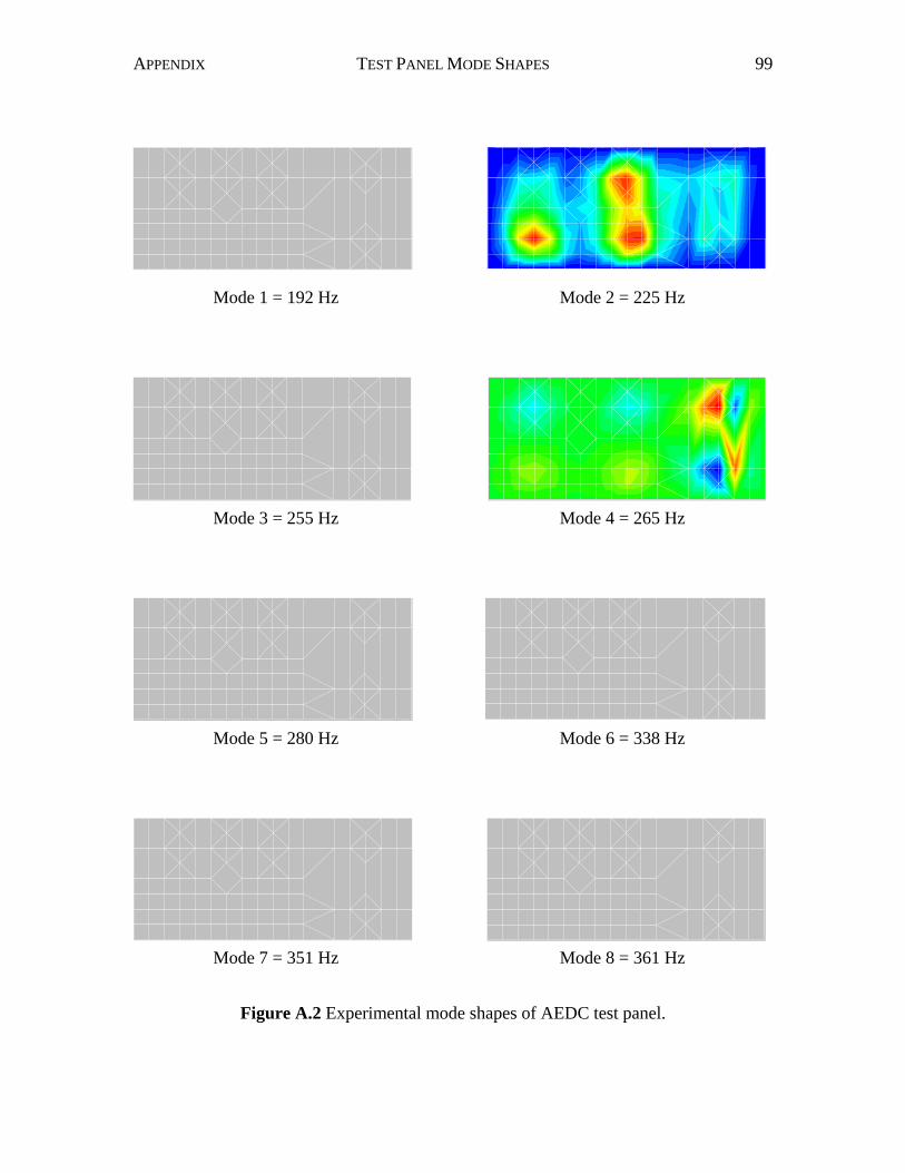
APPENDIX TEST PANEL MODE SHAPES 99
Mode 1 = 192 Hz Mode 2 = 225 Hz
Mode 3 = 255 Hz Mode 4 = 265 Hz
Mode 5 = 280 Hz Mode 6 = 338 Hz
Mode 7 = 351 Hz Mode 8 = 361 Hz
Figure A.2 Experimental mode shapes of AEDC test panel.
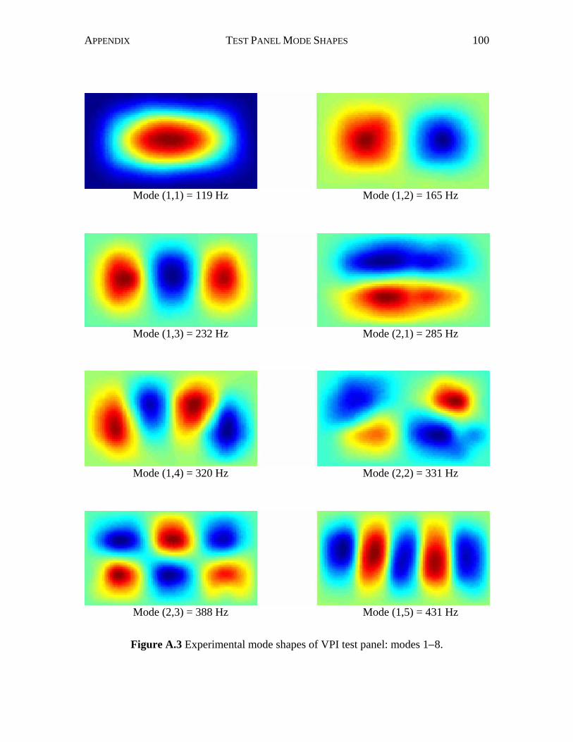
APPENDIX TEST PANEL MODE SHAPES 100
Mode (1,1) = 119 Hz Mode (1,2) = 165 Hz
Mode (1,3) = 232 Hz Mode (2,1) = 285 Hz
Mode (1,4) = 320 Hz Mode (2,2) = 331 Hz
Mode (2,3) = 388 Hz Mode (1,5) = 431 Hz
Figure A.3 Experimental mode shapes of VPI test panel: modes 1−8.
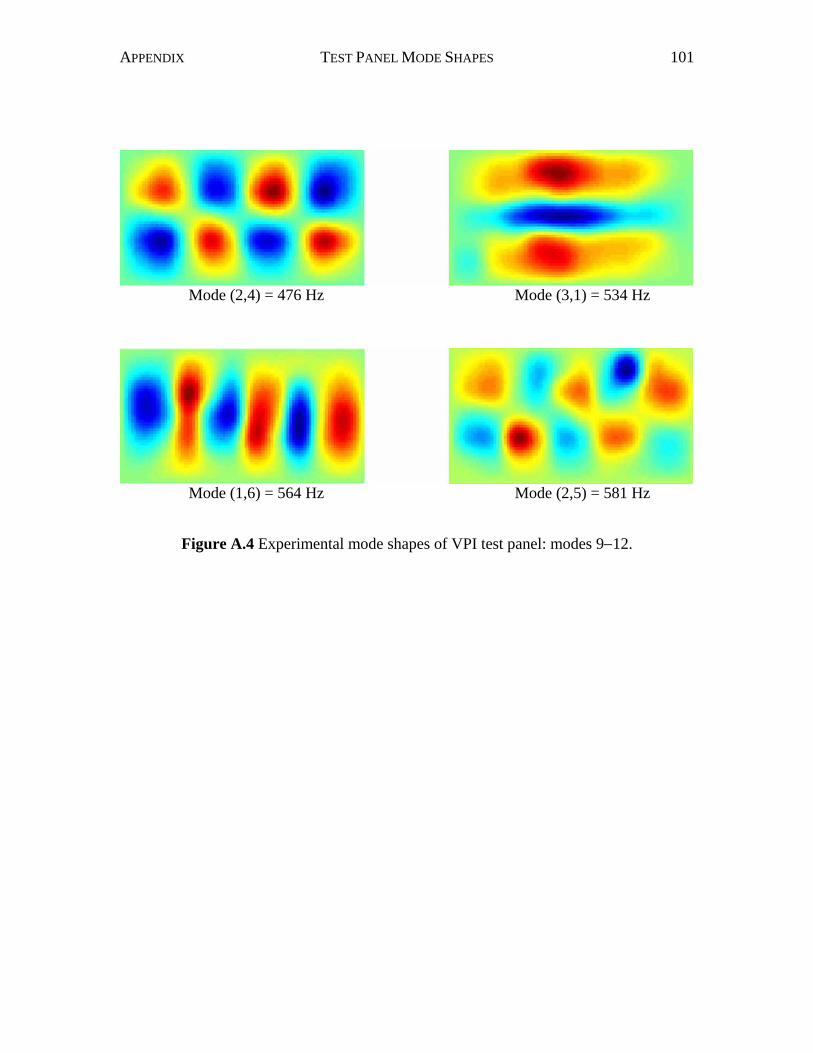
APPENDIX TEST PANEL MODE SHAPES 101
Mode (2,4) = 476 Hz Mode (3,1) = 534 Hz
Mode (1,6) = 564 Hz Mode (2,5) = 581 Hz
Figure A.4 Experimental mode shapes of VPI test panel: modes 9−12.
102
Vita Jason R. Griffin was born on March 25, 1972 in an Army hospital in Alexandria,
Virginia. Several years later he moved to Waynesboro, Virginia where he spent the rest
of his childhood. Jason graduated in June of 1990 from Stuarts Draft High School and
began his undergraduate studies that following August in Mechanical Engineering at
Virginia Polytechnic Institute and State University. In December of 1994 he received his
B.S. in Mechanical Engineering and began working temporarily at Litton Poly-scientific
in Blacksburg, Virginia while his wife finished her degree. In August of 1995 Jason took
a job in Colonial Heights, Virginia designing commercial refrigerated display cases for
Hill PHOENIX. Two years later Jason returned to Virginia Polytechnic Institute and
State University to begin his work on a Master of Science in Mechanical Engineering.
Both years of graduate school were spent working in the Vibration and Acoustics
Laboratories (VAL) under the direction of Dr. Chris R. Fuller. In August of 1999 Jason
began work with Cummins Engine Company working as a Mechanical Development
Engineer.