the consumption e ects of the 2007-2008 financial crisis ... · financial crisis: evidence from...

The Consumption Effects of the 2007-2008

Financial Crisis:

Evidence from Households in Denmark∗

Thais Lærkholm Jensen†

and

Niels Johannesen‡

November 2016

Abstract

Did the financial crisis in 2007-2008 spread from distressed banks to house-

holds through a contraction of the credit supply? We study this question with

a dataset that contains observations on all accounts in Danish banks as well

as comprehensive information about individual account holders and banks. We

document that banks exposed to the financial crisis reduced their lending rel-

ative to non-exposed banks, which in turn caused a significant decrease in

the borrowing and spending of their customers. The effects were persistent:

borrowing remained lower through the post-crisis years and spending foregone

during the crisis was not recovered.

∗We thank John Campbell, Samuel Hanson, Rajkamal Iyer, Jonathan Parker, Atif Mian, Søren Leth-Petersen, Ra-

mana Nanda, Victoria Ivashini, Jose-Luis Peydro, Martin Simmler and Adi Sundaram along with seminar participants

at Harvard Business School, MIT Sloan School of Management, Norwegian Business School, Pompeu Fabra University

and the University of Copenhagen for helpful comments and suggestions. We acknowledge generous financial support

from the Economic Policy Research Network. Part of the research was carried out while Thais Lærkholm Jensen and

Niels Johannesen were visiting researchers at Harvard Business School and the University of Michigan respectively

and the hospitality of these institutions is gratefully acknowledged. The viewpoints expressed in this paper do not

necessarily reflect those of the Danish Central Bank. All errors are our own.†Department of Economics, University of Copenhagen, Øster Farimagsgade 5, DK-1353 Copenhagen K and Dan-

marks Nationalbank, Havnegade 5, DK-1093 Copenhagen K. E-mail: [email protected]‡Department of Economics, University of Copenhagen, Øster Farimagsgade 5, DK-1353 Copenhagen K. E-mail:

[email protected]

1 Introduction

The global banking crisis in 2007-2008 was followed by the Great Recession where

corporate investment, employment and household consumption fell sharply in vir-

tually all developed countries. This pattern of a financial bust followed by a severe

contraction of the real economy has played out numerous times over the last centuries

(Reinhart & Rogoff, 2009).

A central question faced by economists trying to grasp the dynamics of the Great

Recession is whether the crisis in the banking sector was transmitted to the real

economy through a reduction in credit supply. The tightening of credit by banks

in financial distress is one among several possible explanations why firms stopped

investing and households slashed consumption in the aftermath of the financial crisis.

Understanding the strength of this transmission mechanism is important for guiding

policy responses to future crises. To the extent that tightened credit is responsible

for the transmission to the real economy, it may be possible to contain a financial

crisis by securing credit to the firms and households served by banks in distress.

This paper explores how the financial crisis in 2007-2008 affected the borrowing

and consumption of households through the credit supply channel. Our laboratory

is Denmark where households, like in the U.S. and many other advanced economies,

are highly levered and thus depend strongly on credit to sustain consumption.

We exploit a unique dataset from the Danish tax authorities, which contains

information about the balance of all loan accounts in Danish financial institutions

for the period 2003-2011, and add comprehensive information about account holders

from administrative records as well as balance sheet information about banks. We can

thus track the borrowing of households in each bank and assess the extent to which

they reduced total borrowing or compensated with borrowing from other banks when

their existing bank tightened credit. We can also estimate the effects on real estate

and automobile choices as well as total spending imputed from income and wealth

information (Browning & Leth-Petersen, 2003).

Our empirical strategy exploits that the financial crisis in 2007-2008 affected Dan-

ish banks differentially depending on the structure of their balance sheet. While the

origin of the crisis was losses on US mortgage-backed securities, it spread within the

banking sector through the markets for short-term funding (Brunnermeier, 2009; Shin,

2009; Gorton & Metrick, 2012). Danish banks generally had limited direct exposure

to US mortgage-backed securities (Rangvid, 2013), however, those that relied heav-

ily on wholesale funding experienced a severe liquidity shock when funding markets

2

froze in 2008. Hence, the financial crisis plausibly induced a differential credit supply

shock to Danish households because banks with a stable funding base and relatively

liquid assets were able to continue lending as before, whereas banks with an unstable

funding base and relatively illiquid assets were forced to reduce their lending.

Based on these considerations, we measure a bank’s exposure to the financial cri-

sis as the ratio of loans to deposits in 2007 where the denominator reflects relatively

illiquid assets and the denominator reflects relatively stable funding. We provide two

types of evidence that banks with more exposure reduced their supply of credit rela-

tive to banks with less exposure. First, in a simple bank-level analysis, we show that

more exposure was associated with a significantly larger decrease in lending over the

period 2008-2011. This finding mirrors existing studies of lending dynamics during

the financial crisis (Ivashina & Scharfstein, 2010; Cornett et al., 2011) and is clearly

consistent with a differential tightening of the credit supply. Second, in the subsam-

ple of individuals with loan accounts in multiple banks, we conduct a conceptually

similar exercise at the account-level. With credit demand shocks being fully absorbed

by individual-time fixed effects, our finding that banks with more exposure reduced

lending during the financial crisis relative to banks with less exposure must derive

from a differential change in the credit supply (Khwaja & Mian, 2008).

In the main analysis, we exploit this variation in the credit supply to identify how

the financial crisis affected households through the credit supply channel. We match

each individual with their primary bank in 2007 and ask whether customers in banks

that were more exposed to the imminent financial crisis fared worse through the crisis

and post-crisis period in terms of credit and consumption. Specifically, we compare

the outcomes of customers in banks with above-median exposure (“exposed banks”)

to the outcomes of customers in banks with below-median exposure (“non-exposed

banks”). This difference-in-difference estimator identifies the direct effect of the credit

supply shock on customers in exposed banks, but not the general equilibrium effects

that are likely to be similar for customers in all banks.

The key challenge for identification is that banks’ exposure to the financial crisis

may conceivably correlate with the credit demand of their customers. Such a correla-

tion could arise if exposed banks were also characterized by other imprudent business

practices such as low credit standards and lax monitoring of borrowers. This could

cause selection into exposed banks by inherently impatient individuals who borrowed

beyond their means before the crisis and thus demanded less credit after the crisis. In

this example, simply comparing the credit outcomes of customers in exposed and non-

exposed banks would conflate demand and supply factors and therefore not correctly

3

identify the credit supply channel.

We address this identification issue in various ways. First, we show that the ob-

servable characteristics of customers in exposed and non-exposed banks are virtually

identical. Seemingly, the two types of banks served the same household segments at

the eve of the crisis suggesting that they were exposed to the same demand shocks.

Second, our model eliminates several confounding factors by including individual fixed

effects as well as a comprehensive set of pre-crisis individual characteristics interacted

with time dummies. For instance, non-parametric controls for the pre-crisis distri-

bution of debt interacted with time dummies effectively control for differential credit

demand shocks arising from differences in pre-crisis leverage (Dynan et al., 2012). In a

similar way, we eliminate credit demand shocks arising from differences in municipal-

ity, industry, income, age, education and so on. Third, we show that pre-crisis trends

in outcomes are parallel across individuals whose banks were exposed differently to

the crisis. This strengthens the case that also unobservable individual characteristics

affecting credit demand are uncorrelated with bank exposure.

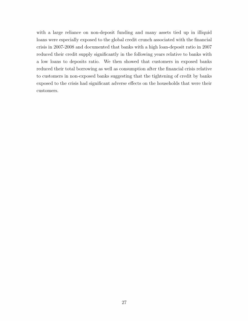
The first set of results provides strong evidence that the financial crisis reduced

household borrowing through the credit supply channel. The total debt of customers

in exposed banks decreased by around DKK 12,000 (USD 2,000) relative to customers

in non-exposed banks over the period 2008-2009 and this difference persisted through

the period 2010-2011. The drop in total debt reflects a large decrease in credit from

the pre-crisis primary bank and a smaller increase in credit from other banks, which

implies that around half of the decrease in lending by exposed banks was neutralized

by their customers borrowing more in other banks.

The relative decrease in the quantity of credit to customers in exposed banks was

accompanied by a relative increase in the price of credit. In a sample of newly issued

consumer loans where we can infer that loan terms are comparable, we document

a differential increase in the effective interest rate of around 0.75 percentage point

in 2008-2009. The finding that price and quantity moved in opposite directions is

consistent with a shift in supply, but not with a shift in demand.

We also present evidence suggesting that the tightening of credit imposed effective

borrowing constraints on some households. Most employees in Denmark have a tax

favored pension savings account funded by mandatory employer contributions, how-

ever, a steep penalty for liquidation makes this an undesirable source of liquidity for

individuals with access to credit. We show that the propensity to liquidate pension

accounts increased significantly for customers in exposed banks relative to customers

in non-exposed banks during the crisis. Although the absolute number of liquidations

4

remained modest, the result is suggestive that customers in exposed banks were more

likely to experience severe borrowing constraints.

The second set of results shows that the decrease in borrowing was accompanied by

a significant decrease in consumption. The annual spending of customers in exposed

banks decreased by almost DKK 8,500 (USD 1,400) relative to customers in non-

exposed banks between 2007 and 2009. Part of this effect reflects a decrease in

spending on real estate: customers in exposed banks bought smaller and less expensive

houses relative to customers in non-exposed banks. But other consumption margins

adjusted too: customers in exposed banks became less likely to be car owners and

less likely to own multiple cars relative to customers in non-exposed banks.

Since spending decisions in different time periods are tied together by the in-

tertemporal budget constraint, we should expect a relatively low level of spending

during the crisis to be matched by a relatively high level of spending in later years.

We find that customers in exposed banks returned to the spending path of customers

in non-exposed banks in the post-crisis years 2010-2011; however, we find no evi-

dence that they recovered any of the spending foregone during the crisis. This may

reflect that the credit supply of exposed banks remained low after the crisis or, al-

ternatively, that consumption did not adjust flexibly to a normalization of the credit

supply. Concretely, to the extent that households acquired less expensive homes and

cars during the crisis because of a low credit supply, habit and transaction costs may

have prevented them from adjusting these consumption margins as the credit supply

normalized.

The final set of results suggests that the effects of the credit supply shock were

heterogeneous across customers in exposed banks with those holding less liquidity at

the eve of the crisis being more adversely affected. While the differential decrease in

total debt after 2007 was large and persistent within the bottom quintile of pre-crisis

liquidity, it was small and temporary within the top quintile. Consistent with these

results, we find a negative effect on spending within the bottom quintile of liquidity

in every year of the crisis and post-crisis period, but no clear evidence that spending

within the top quintile was affected at all.

While our empirical results are difficult to reconcile with theoretical models of

frictionless banking markets, they are consistent with different types of frictions: a

cost of switching banks on the customer-side (Klemperer, 1987), which makes some

individuals stay with their existing bank even when they could have obtained better

credit outcomes in other banks, and imperfect information on the bank-side, which

creates ex ante uncertainty about default probabilities (Sharpe, 1990) and deters

5

banks from lending to new customers. Both frictions imply that customers in exposed

banks on average obtain less credit than they would have as customers in non-exposed

banks.

In practice, it is improbable that imperfect information plays a major role in

the Danish market for consumer loans: households have relatively simple balance

sheets and banks have access to comprehensive information about the income and

credit histories of potential customers. It seems more likely that the relevant friction

is on the customer-side, which is consistent with recent evidence that households

make costly mistakes in loan markets. For instance, it has been shown in the U.S.

context that shopping from too few mortgage brokers costs the average borrower

around $1,000 (Woodward & Hall, 2012) and that the frequently observed failure to

refinance mortgage loans entails costs of around $11,500 in present value terms (Keys

et al., 2016).

The main contribution of the paper is to enhance our understanding of the sharp

decrease in household consumption that often follows a financial crisis. Existing

studies emphasize the role of excessive leverage (Mian & Sufi, 2010), falling house

prices (Mian et al., 2013) and increased uncertainty (Alan et al., 2012) whereas our

analysis points to a complementary channel through the contracted credit supply of

distressed banks.

The existing literature linking financial crises to household outcomes through the

credit supply channel is small and has produced mixed results. Two papers show

that banks with high exposure to the 2007-2008 financial crisis reduced their lending

to households in its aftermath (Ramcharan et al., 2015; Puri et al., 2011). While

these findings suggest that the credit supply channel contributed to the drop in con-

sumer demand for housing and automobiles after the financial crisis, the papers only

consider bank-level outcomes and therefore cannot determine whether customers in

exposed banks were able to compensate with borrowing from other sources and thus

ultimately maintain their desired level of consumption. One paper addresses this is-

sue by combining bank and household survey data from Canada and concludes that

the financial crisis had no effect on household consumption through the credit supply

channel (Damar et al., 2014).1

While our measure of spending is not directly comparable to the notion of pri-

vate consumption in national accounts, the estimated effect on spending suggests

1The credit supply channel is more thoroughly documented in the context of firms. A number ofpapers demonstrate that firms’ borrowing decreases when their bank relation is in distress (Khwaja& Mian, 2008; Jimenez et al., 2014) and point to real effects in terms of reduced investment (Kleinet al., 2002; Dwenger et al., 2015) and employment (Chodorow-Reich, 2014; Bentolila et al., 2015).

6

that credit supply was a quantitatively important factor in the collapse of household

consumption after the financial crisis. To illustrate, the estimates imply that being

a customer in a bank exposed to the crisis in 2007 lowered spending at the sample

mean by more than 4% in 2009. Embedded in a general equilibrium framework, our

micro estimates could help quantifying how financial shocks shape macro-economic

outcomes.

The paper proceeds in the following way. Section 2 provides background informa-

tion on the banking sector and the financial crisis in Denmark. Section 3 describes

the data sources and reports summary statistics. Section 4 documents the differential

credit supply shock. Section 5 discusses the empirical strategy. Sections 6-8 present

the results concerning financial outcomes, consumption outcomes and heterogeneous

effects respectively. Section 9 concludes.

2 Background

2.1 The Danish financial sector

The Danish financial sector counts more than 100 retail banks, however, the bank

market is relatively concentrated: 4 systemically important banks account for the

majority of all lending while the remaining banks are predominantly regional or local

banks.

All banks in Denmark rely on information from both public and private sources to

assess credit risk. First, there is an automated procedure for banks to obtain financial

information about loan applicants directly from the tax authorities. With the consent

of the applicants, banks can access data on income and debt from tax returns as

well as information on arrears to the public sector. Second, banks universally acquire

information on arrears to private creditors from commercial registers and credit scores

(similar to FICO scores) are readily available from credit bureaus.

Based on the availability of hard information about loan applicants, it seems un-

likely that informational barriers to bank switches should be larger in Denmark than

in other developed countries. This is consistent with survey evidence that customer

mobility in Denmark, while low in absolute terms, is high by international standards:

3.6% of Danish survey respondents formed a new primary bank relation in 2013 com-

pared to 3.6% in the U.S., 2.5% in Germany, 2.4% in the U.K and only 1% in the

Netherlands (Bain & Co, 2013).

The most distinctive feature of the Danish financial sector is the important role

played by specialized mortgage credit institutions. These institutions are much more

7

regulated than retail banks. They are only allowed to lend with collateral in Danish

real estate and the loan-asset ratio on their loans cannot exceed 80% at origination.

Moreover, they must be fully funded with publicly traded bonds and are required to

lend at the interest rate at which they borrow plus a fixed premium covering average

credit risk.

While consumer and auto loans are typically granted by banks and never involve

mortgage credit institutions, most real estate purchases are financed with credit from

both sources: a senior loan from a mortgage credit institution up to the regulatory

limit and a junior loan from a bank that finances the residual. This implies that

banks are typically the marginal providers of mortgage credit to households and that

the credit limit set by banks determines the total amount of mortgage credit available

to their customers. We therefore focus on the role of banks’ credit supply in shaping

credit and consumption outcomes of households.

2.2 The financial crisis 2007-2008 and its aftermath

In the years before the global financial crisis in 2007-2008, the Danish economy was

growing at a rapid pace, the real estate market was booming and banks expanded

their lending substantially. Since lending grew much faster than deposits, some banks

relied increasingly on international credit markets to finance their expansion, often

through loans at short maturities IMF (2014).

While Danish banks generally had very limited exposure to the U.S. mortgage-

backed securities that triggered the financial crisis, some banks reached dangerously

low levels of liquidity when global markets for wholesale funding froze (Rangvid,

2013; Shin, 2009). Between May and September 2008, the central bank therefore

intervened several times to provide liquidity to the banking system and in October

2008, shortly after the collapse of Lehmann Brothers, the government was compelled

to extend a two-year unlimited guarantee to all bank liabilities. Despite the massive

efforts to sustain the financial sector, many banks were in serious distress: 15 banks

were closed by the regulatory authorities between 2008 and 2011 and many others

accepted mergers to avoid failure reducing the total number of licensed banks from

147 in 2007 to 113 in 2011 (Rangvid, 2013).

A severe crisis in the real economy accompanied and aggravated the banking crisis.

Between 2007 and 2009, real private consumption decreased by around 4%, real GDP

by around 5%, real investment by around 18%, real housing prices by around 20%

and stock prices by more than 40%.

8

Figure 1 tracks our two key outcomes, household borrowing and consumption,

over the boom and bust.2 It shows a rapid increase in both outcomes until the peak

of the financial crisis in 2008 when the expansion of credit suddenly came to a halt and

consumption dropped sharply. The timing is suggestive of a causal relationship: the

credit expansion stopped in the first quarter of 2008 and consumption started falling

a few quarters later. The goal of the paper is to investigate whether the decline in

credit and consumption can be explained with a decrease in banks’ credit supply.

[Figure 1 around here]

3 Data

3.1 Data sources

The main data innovation of this paper is to establish a link between individuals

and their bank relations from tax records. At the end of each year, financial institu-

tions in Denmark report the balance of their customers’ deposit and loan accounts to

the tax authorities. The reports are compulsory and reliable since they are used for

tax enforcement. We thus have a complete mapping of all loans and deposits with

domestic financial institutions held by all individuals in Denmark.3

To the raw administrative records of the Danish tax authorities, we add com-

prehensive information about the individual account holders from a number of other

administrative registers. This includes demographic information such as age, gen-

der, education, home municipality and identity of children and parents; labor market

information such as wage income, industry and unemployment spells; income and

wealth information such as capital income, social transfers, value of stock portfolios

2The analysis is conducted on the basis of the MFI Statistics published by the Danish CentralBank, which excludes the smallest banks; hence, the number of banks is lower than the total numberof licensed banks reported above. The excluded banks, however, account for less than 1% of totalbank lending.

3In practice, we obtain the link between individuals and banks in the following way. The first fourdigits of the bank account numbers that we observe in the tax records uniquely identify the branchof the bank where the accounts are held in a given year. We then hand-collect lists of branch id-numbers and the corresponding banks from publications by Nets, a payment solutions provider, foreach of the years 2003-2011. This establishes the dynamic link between individual account numbersand bank identity.

9

and pension accounts; auto register information such as the weight and production

year of each registered automobile; real estate register information such as the size

and value of each registered property. We also add detailed balance sheet information

about the reporting banks obtained from the Danish Central Bank.

In the resulting dataset, we thus observe the following information for all individ-

uals resident in Denmark for the period 2003-2011: the balance of each of their loan

and deposit accounts; balance sheet information about the bank in which the account

is held; and comprehensive background information about individual account holders

from government registers.

3.2 Imputed spending

One of our key outcomes is spending, which we impute from income and wealth

variables. The main idea is that spending in a given period, by definition, equals

disposable income minus the increase in net wealth. Hence, to the extent that dispos-

able income and wealth can be measured precisely, it is possible to impute spending

as:

spendingit = disposable incomeit − (net wealthit − net wealthit−1) (1)

While several papers validate the imputed measure of spending by showing that it

correlates strongly with survey measures of consumption (Browning & Leth-Petersen,

2003; Kreiner et al., 2014), the imputation method also has limitations. Most im-

portantly, an increase in stock prices tends to lower measured spending by creating

an increase in net wealth that is not matched by an increase in disposable income

(unless the capital gain is realized). Similarly, an increase in the market interest rate

reduces the market value of fixed-rate mortgage loans, which increases net wealth and

lowers measured spending. In both cases, the imputation method confounds changes

in valuation of balance sheet components with true savings. By contrast, refinancing

of mortgage loans, whereby one loan is replaced by another with the same market

value, does not affect measured spending.

We address these measurement problems in the following ways. For stock own-

ers, we use the evolution of the general stock market index to estimate the change

in portfolio values that is induced by price changes and add it back into imputed

spending. With this procedure, stock price changes do not lead to mismeasurement

of spending for individuals who hold the market portfolio, but will cause it to be

overestimated (underestimated) for individuals whose stock portfolio underperforms

(overperforms) relative to the market portfolio. Additionally, we conduct robustness

tests where all stock owners are excluded; in this sample there is clearly no valuation

10

effect of stock prices on measured spending. Similarly, in other robustness tests, we

exclude all owners of real estate; in this sample there is no valuation effect of market

interest rates because borrowing for other purposes than real estate takes the form of

variable-rate loans whose market value is independent of market interest rates.

It is natural to compare our imputed measure of spending to the measure of pri-

vate consumption employed in national accounts. The main difference between the

two measures is the way they treat owner-occupied housing. Our spending measure

includes expenses related to purchases and renovation of real estate. Technically, this

is achieved by omitting real estate from net wealth in the imputation of spending:

when households purchase real estate or incur expenses related to renovation, this

concept of net wealth decreases by the full amount of the expense, through a decrease

in financial assets if financed with own funds or an increase in liabilities if financed

with debt, and their imputed spending increases correspondingly.4 By contrast, na-

tional accounts define consumption of owner-occupied housing as the market rent and

ignore any cash spending.

Despite this conceptual difference, the two measures are empirically very similar

when aggregated to the population-level. As shown in Figure 2, imputed spending

grew slightly faster than private consumption before the financial crisis and dropped

slightly more after, but both the level of the two measures and their trend over time

are quite alike.


3.3 Sample and summary statistics

Before conducting the empirical analysis, we restrict the sample in several ways.

First, we remove self-employed individuals since it is generally not possible to separate

borrowing for business and private purposes on the balance sheet of those operating

a firm in their own name. Second, we restrict the sample to individuals between

20 and 50 years (in 2007), which is the time in the life-cycle where credit plays the

most important role in supporting spending. Third, we exclude individuals whose

4A measure of non-real estate spending could, in principle, be obtained by including the marketvalue of real estate in net wealth. In our dataset, we observe the assessed value of real estate fortax purposes, which is lower than the market value by a margin that varies over time and acrossregions. Simply including the assessed value of real estate in net wealth therefore yields a spendingmeasure that is difficult to interpret because it includes some but not all real estate spending.

11

primary bank in 2007 failed during the period 2008-2011; since failed banks were

typically absorbed by sound banks and all customer accounts were transferred in the

process, such individuals received a fundamentally different treatment than customers

in exposed but surviving banks. Finally, we study a 25% random sample of the

resulting population for computational tractability. These restrictions leave us with

a baseline sample of around 440,000 individuals, almost 3.5 million individual-years

and more than 5.7 million individual-account-years.

Once the dataset is constructed, we define a unique primary bank for each indi-

vidual in 2007 using the following procedure:5 For individuals who only had one bank

relation in 2007, this is their primary bank. For individuals who had multiple bank

relations in 2007, but only had a loan in one of those banks, this is their primary

bank. For individuals who had loans in multiple banks in 2007, the bank in which the

loan balance was largest is their primary bank. For individuals who had no loans, but

had deposits in multiple banks in 2007, the bank in which the deposit balance was

largest is their primary bank. The procedure thus rests on the assumptions that loans

provide a stronger bank relation than deposits and that bank relations are stronger

the larger the account balance.

Next, we order individuals according to the loan-deposits ratio of their primary

bank in 2007 and split the sample at the median individual so that the number of

individuals with exposed and non-exposed banks is approximately the same.6

Table 1 reports pre-crisis summary statistics on the main variables used in the

analysis for customers in banks with high and low ratios of loans to deposits sepa-

rately. All variables measured in DKK are winsorized at the 1st and 99th percentiles

to reduce the influence of extreme observations. The first column provides a sense

of the demographic characteristics and financial situation of the individuals in our

sample. Individuals were roughly equally distributed across the four education cate-

gories, around two thirds had a cohabitating partner and more than half had children.

The average total income was around DKK 250,000 (USD 35,000) and the average

disposable income after taxes and interest payments around DKK 200,000. Since the

average imputed spending was around DKK 220,000, we can infer that the average in-

dividual reduced net wealth by around DKK 20,000 in 2007. The average level of debt

was around DKK 500,000 (USD 70,000) implying a ratio of debt to income around 2,

which is very high by international standards and higher than in, for instance, the U.S.

5To be precise, the primary bank is always a bank and not a mortgage institution.6The small discrepancy is due to the fact that the individuals right below and right above the

median who are customers in the same bank are assigned to the same group.

12

[Table 1 around here]

The next columns serve to assess whether customers in exposed and non-exposed

were different with respect to their pre-crisis observed characteristics and, hence,

whether it is likely that divergence between the two groups in the crisis and post-

crisis period was driven by differential credit demand shocks. This does not seem to

be the case. Table 1 shows that customers in banks with high and low loan-deposit

ratios were strikingly similar. None of the differences between variable means in the

two samples are close to statistical significance. Hence, there are no signs of customer

selection into exposed banks based on observable household characteristics.

Finally, the table illustrates the important role of specialized mortgage credit

institutions: around one third of household loans in Denmark are from banks while

the remaining two thirds is from mortgage credit institutions. Although our empirical

strategy only exploits variation in the credit supply of banks, the significance of non-

bank debt points to total debt as the main financial outcome of interest. Given

the institutional framework explained in section 2.1, we expect loans from banks

and mortgage credit institutions to be complements: since bank customers typically

cannot increase the share of financing from mortgage credit institutions in response to

a tightening of bank credit, they are likely to purchase less real estate, which reduces

borrowing from both banks and mortgage credit institutions in absolute terms.

4 The differential credit supply shock

The main premise of our analysis is that banks with fewer deposits on the liability

side of their balance sheet and more loans on the asset side, tightened their credit

supply more in response to the financial crisis. This section provides two types of

evidence, based on bank-level and account-level data respectively, in support of this

premise.

4.1 Bank-level analysis

Figure 3 compares the trend in lending through the financial crisis for banks with a

ratio of loans to deposits above and below the sample median in 2007. While the

two groups of banks exhibited very similar growth rates in lending during the period

2005-2007, there was a sharp divergence over the period 2008-2012: whereas banks

13

with a low loan-deposit ratio continued to expand lending, banks with a high loan-

deposit ratio reduced lending considerably in a sudden reversal of the trend in the

previous years. Table 2 shows that the negative correlation between banks’ pre-crisis

loan-deposit ratio and subsequent growth in lending is statistically significant, re-

gardless of whether the regressions are unweighted or weighted with bank size and

whether the loan-deposit ratio is used as a continuous variable or transformed into a

dummy variable indicating a loan-deposit ratio above the median. These results are

in line with existing studies of bank lending during the financial crisis (Ivashina &

Scharfstein, 2010; Cornett et al., 2011).7



4.2 Loan-level analysis

While the bank-level results are consistent with a differential credit supply shock, it

cannot a priori be excluded that they are in fact driven by differential credit demand

shocks; strictly speaking it could be customers’ demand for credit that for one reason

or the other correlated with banks’ loan-deposit ratios rather than banks’ supply of

credit.

To cleanly establish the existence of a differential credit supply shock, we conduct

an account-level analysis exploiting that individuals with loan accounts in multiple

banks create within-individual variation in loan outcomes. Intuitively, if individuals

with loan accounts in both exposed and non-exposed banks systematically became

less likely to obtain new credit in exposed banks than in non-exposed banks after

the financial crisis, this cannot be explained with changes in credit demand but must

reflect a differential change in credit supply. Formally, we estimate the following

account-level model:

newloanibt = θit + φΩt × exposedb + µibt (2)

7Figure A1 in the Appendix shows how the mean loan-deposit ratio evolves over the sample periodfor banks with a loan-deposit ratio above and below the median in 2007: the difference between thetwo means is roughly constant until 2008 with some convergence in the later years as banks with ahigh initial loan-deposit ratio reduces this ratio significantly.

14

The dependent variable newloanibt indicates if individual i increased borrowing in

bank b at time t; θit represents individual-time fixed effects; Ωt is a vector of time

dummies; and exposedb indicates if bank b had a loan-deposit ratio above the median

in 2007. The model includes no covariates since individual characteristics are fully

absorbed by the individual-time fixed effects.

The parameter of interest φ, measures how much more likely it is that a new loan

is taken out in an exposed bank than in a non-exposed banks when borrowers have

loan accounts in both (measured relative to 2007). Since individual-year fixed effects

absorb the credit demand of each individual at each point in time, any differential

change in the likelihood of taking out new loans across banks with different exposure

can be attributed to differential changes in the credit supply. This is an application

of the within-estimator proposed by Khwaja & Mian (2008).

Figure 4 illustrates the results by plotting the estimated coefficients on the inter-

actions between exposed and the year dummies (i.e. the elements in the vector φ).

The coefficients for the years 2004-2006 are very close to zero, which implies that, in

the sample of individuals with loan accounts in both exposed and non-exposed banks,

the likelihood of increasing the loan balance in the former relative to the latter was

constant throughout the pre-crisis period. The coefficient for 2009 is statistically sig-

nificant and the point estimate implies that individuals in the sample, who increased

the balance of any loan account, were 15 percentage points less likely to do so in an

exposed bank than in a non-exposed bank. For 2010 and 2011, the point estimates

are also negative, but not statistically significant. Overall, this suggests that the

credit supply of banks exposed to the financial crisis decreased sharply relative to

non-exposed banks in 2009 and plausibly remained lower throughout the post-crisis

period.


While the analysis in this section provides clean evidence of a differential credit

supply shock, the findings do not imply that customers in exposed banks were ad-

versely affected; neither the bank-level or the account-level results exclude that the

differential credit supply shock was neutralized by customers switching from exposed

to non-exposed banks. For this reason, our main analysis studies outcomes at the

individual level. This allows us to study the full effect of the differential credit supply

shock on bank customers while taking into account substitution toward other sources

of credit.

15

5 Empirical strategy

The main aim of the empirical analysis is to estimate the effect of banks’ credit

supply on the credit and consumption outcomes of households. Our empirical strategy

is to compare individuals, whose primary bank was exposed to the financial crisis

and therefore reduced its credit supply, to individuals whose primary bank was less

exposed. We implement this comparison with the following baseline model:

outcomeit = αi + γΩt + βΩt × exposedi + δΩt ×Xi + εit (3)

where outcomeit is a financial or consumption outcome of individual i at time t; αi

represents individual fixed effects; Ωt is a vector of time dummies (2007 is the omitted

category); exposedi is a dummy variable indicating if the primary bank of individual

i in 2007 had a loan-deposit ratio above the population median; and Xi is a vector of

characteristics of individual i in 2007.

The vector β contains the main coefficients of interest. For each year it measures

the average change in the outcome variable relative to 2007 for individuals who were

customers in exposed banks in 2007 over and above the average change over the

same period for individuals who were customers in non-exposed banks. The baseline

model thus yields difference-in-difference estimates of how the financial crisis affected

households through the credit supply channel for each of the years 2008-2011.

For expositional simplicity, we sometimes employ a compact version of the model

where outcomes are averaged within the periods 2005-2007 (“pre-crisis”), 2009 (“cri-

sis”) and 2010-2011 (“post-crisis”). With the dataset collapsed to only three time

periods, the difference-in-difference estimates are expressed by the interaction terms

exposed × crisis and exposed × post − crisis. Whenever we employ the compact

model, we always report the results from the full baseline model in Table A1 in the

Appendix.

The main methodological challenge is the possibility that credit demand shocks

correlate with the credit supply shock. For instance, it may be that customers in

exposed banks incidentally had educational backgrounds, lived in geographical regions

or worked in industries that made them more affected by the crisis through other

channels. Alternatively, they may have had different unobserved characteristics, such

as risk attitudes or time preferences, which made them behave differently during

the crisis. In either case, the credit demand shocks of individuals may have varied

systematically with the exposure of their bank, which invalidates identification of the

credit supply channel based on a simple comparison of customers in exposed and

16

non-exposed banks. We address this identification issue in two ways.

First, the difference-in-difference estimates are conditional on a comprehensive

set of controls. For each control variable, we include the value in 2007 as well as

its interactions with year dummies. With this procedure we effectively identify the

effect from a comparison of individuals with the same observed characteristics in 2007,

of which some were customers in exposed banks and others were customers in non-

exposed banks. The baseline model includes 161 covariates (all interacted with a full

set of time dummies) that capture the following characteristics: gender (dummy for

being a woman), age (dummies for each 1-year age group), education (dummies for

short, medium and long education with no education as the omitted category), home

ownership (dummy for owning real estate), children (dummy for having children),

civil status (dummy for cohabitation with partner), student (dummy for being a

student), unemployment (dummy for unemployment spells during 2006-2007), bank

debt (dummies for the deciles of the bank debt distribution in 2007), income (dummies

for the deciles of the income distribution in 2007), home municipality (dummy for

each of 98 Danish municipalities), and industry (dummy for each of 9 occupation

sectors).

Second, β allows us to assess directly whether customers in exposed and non-

exposed banks followed similar trajectories in terms of borrowing and consumption

over the period 2003-2007 conditional on observed characteristics. To the extent that

trends in outcomes are parallel during a period where there were no major differential

shocks to credit supply, it is at least suggestive that the unobserved characteristics

shaping credit demand are roughly balanced across customers in the two types of

banks.

While the baseline specifications use a dichotomous measure of bank exposure

to the financial crisis, our results are generally very similar when we replace exposed

with the loan-deposit ratio and thus use the variation in exposure within the groups of

exposed and non-exposed banks. The core results with this specification are reported

in Table A2 in the Appendix.

All point estimates are reported with standard errors clustered at the level of

the primary bank in 2007. This conservative clustering strategy widens the stan-

dard errors considerably given that the baseline sample includes close to 3.5 million

observations at the individual-year level, but only just over 100 banks.

Finally, it is important to bear in mind when interpreting the results that β

measures the “partial equilibrium” effects of the credit supply shock in the sense that

any general equilibrium effects are absorbed by the time dummies. For instance, to

17

the extent that the credit supply shock induced customers in exposed banks to reduce

spending and this, in turn, aggravated the economic crisis with adverse consequences

for all households in the economy, these indirect effects would be included in γ and

not in β. Relatedly, even banks with a low loan-deposit ratio may have tightened

their credit supply because of the financial crisis, although to a lesser extent than

banks with a high loan-deposit ratio, and this part of the credit supply channel is

not included in β since the latter is identified from a comparison of customers in

banks with a high and a low loan-deposit ratio. It should also be noted that we are

effectively studying the dynamic responses to an initial impulse. Exposed and non-

exposed banks had very different loan-deposit ratios before the crisis, but gradually

became more similar as exposed banks reduced their lending. By contrast, customers

in exposed and non-exposed banks were initially very similar, but gradually became

more different as customers in exposed banks accumulated less debt and postponed

desired spending.

6 Results: Financial outcomes

We first use the baseline model with individual fixed effects and a full set of con-

trols to study the main financial outcome: total debt. Figure 5 plots the estimated

coefficients on the interaction terms between the year dummies and the dummy vari-

able indicating that the individual’s primary bank in 2007 was exposed to the financial

crisis (i.e. the elements in the vector β).


For 2004-2006, the point estimates are almost precisely zero suggesting that the

average total debt of customers in exposed and non-exposed banks grew at almost

exactly the same speed before the financial crisis. For 2008-2011, the point estimates

are below zero suggesting that the total debt of customers in exposed banks decreased

relative to the total debt of customers in non-exposed banks after the financial crisis.

Since debt is observed at the end of each year, the gradually decreasing point estimates

of around DKK -4,000 for 2008, DKK -12,000 for 2009 and DKK -15,000 for 2010

imply that most of the divergence occurred in the course of 2009. All point estimates

are statistically and economically significant: the difference-in-difference estimate for

2009 corresponds to around 2.4% of the average level of debt in 2007.

To study how the large set of controls shapes the results, we estimate the com-

pact model while moving sequentially from a specification with no controls, which

18

is essentially a raw comparison of average levels, to the specification will all con-

trols. Column (1) in Table 3 implies that the average total debt was DKK 7,600

higher for customers in exposed banks than for customers in non-exposed banks in

the pre-crisis years whereas it was DKK 6,100 lower at the peak of the crisis in 2009

(a difference-in-difference estimate of DKK -13,700) and DKK 9,900 lower after the

crisis in 2010-2011 (a difference-in-difference estimate of DKK -17,500). To this most

parsimonious specification, Column (2) adds individual covariates; Column (3) fur-

ther adds municipality dummies and industry dummies and Column (4) finally adds

individual fixed effects. In all specifications, the difference-in-difference estimate is

virtually the same, but precision increases considerably as controls are introduced.


We then present similar results for various bank debt outcomes. As shown in

Column (5), customers in exposed banks decreased their total bank debt by around

DKK 7,500 relative to customers in non-exposed banks through the crisis with almost

the entire decrease occurring before the end of 2009. The estimated effects for bank

debt are smaller than for total debt in absolute terms, which confirms our expectation

that loans from banks and mortgage institutes are complements: a reduction in bank

debt induced by tightened bank credit spills over on non-bank debt. Measured relative

to the sample mean, however the estimated effect on bank debt is around 5%, which

is more than twice as large the effect on total debt.

Further, as shown in Columns (6)-(7), the decrease in total bank debt can be

decomposed into a decrease in debt at the bank that served as primary bank in

2007 of around DKK 14,800 and an increase in debt at other banks of around DKK

7,100. This suggests that customers in exposed banks neutralized roughly half of the

differential credit supply by switching to other banks.

A comparison of Columns (4) and (5) shows that almost half of the decrease in

total debt occurred in mortgage institutes. This implies that real estate debt accounts

for a large part of the total effect and ultimately raises the question whether there was

any effect on consumer debt. Since we cannot isolate consumer debt in our dataset,

we apply the baseline model to a subsample of individuals whose entire debt must

be consumer debt: “renters” who did not own real estate at any point during the

sample period. As shown in Column (8), the estimated effect in this subsample is

comparable to the estimated effect on bank debt in the full sample shown in Column

19

(5). This documents that also consumer debt was significantly affected by the credit

supply shock.

While it is consistent with a static and partial equilibrium model of the credit

market that a reduction in the supply causes a decrease in the equilibrium quantity,

the same model also predicts an increase in the equilibrium price. In the next step, we

thus investigate whether interest rates changed differentially for customers in exposed

and non-exposed banks through the crisis.

Since our dataset does not contain explicit information about loan terms, we

compute the effective interest rate in the following way:

interest ratet =interest paidt

0.5(loan balancet−1 + loan balancet)(4)

The main source of error is that we only observe loan balances at the end of each year

and therefore need to approximate the average loan balance in year t with the average

of the loan balances at the end of year t− 1 and year t. This implicitly assumes that

loan balances evolve linearly over the year.

To obtain a meaningful comparison of interest rates, it is crucial to account for

other loan terms, for instance whether the loan is secured with collateral and whether

the rate is variable or fixed. We therefore focus the analysis on a relatively small

sample of newly issued loans where we can infer that other loan terms than the

interest rate are comparable. Specifically, we include an individual in period t in

the estimation sample if three conditions are met: (i) total borrowing is below DKK

1.000 in period t-1; (ii) total borrowing is above DKK 50.000 in period t ; (iii) the

borrower owns no house and no car in period t. Since these borrowers did not own a

house or a car at the time the loans were issued, the loans are likely to be unsecured

consumer loans, which generally have variable interest rates and short maturities.

We validate the procedure by showing that the distribution of estimated interest

rates is sensible (Figure A2 in the Appendix) and that the average effective interest

rate follows the trend of the monetary policy rate closely over time (Figure A3 in the

Appendix). We then apply the baseline model with the modification that individual

fixed effects are not included so as not to restrict identification to the very small

number of individuals who took out multiple loans satisfying the requirements listed

above during the sample period. As shown in Figure 6, the interest rates faced by

customers in exposed and non-exposed followed a very similar trend through the pre-

crisis period, but then diverged sharply in 2009 with customers in exposed banks

experiencing a relative increase in interest rates of around 0.7 percentage points.

20


Having established that the differential credit supply shock induced by the finan-

cial crisis affected credit outcomes in the household sector, we study a number of

related financial outcomes in Table 4. First, when access to credit is constrained,

households may respond by running down financial assets to mitigate the effect on

consumption (Damar et al., 2014). As shown in Column (1)-(2), customers in exposed

banks reduced the value of their bank deposits and stock portfolios only slightly rel-

ative to customers in non-exposed banks through the crisis: the combined decrease

of DKK 1,200 is very modest relative to the corresponding decrease in debt of DKK

14,400 (from Table 3, Column 4) and not statistically significant. However, as shown

in Column (3), the small average effect on liquidity conceals that customers in ex-

posed banks became more likely to reach low levels of liquidity: the probability of

having liquidity below the 25th percentile increased by almost one percentage point

during the crisis for customers in exposed banks relative to customers in non-exposed

banks and the difference persisted through the post-crisis period.8


The finding that exposed banks reduced their credit supply and that their cus-

tomers were unable to compensate fully with credit from other sources suggest that

customers in exposed banks were more likely to become borrowing constrained. We

study this proposition using withdrawals from tax favored pension savings accounts as

an indicator of borrowing constraints. While such accounts are funded by mandatory

employer contributions and thus available to most individuals in Denmark, a 60%

penalty applying to liquidations before pension age makes it a very costly source of

liquidity, which we expect households to use only when alternative sources of liquidity

are exhausted.9 Column (4) documents a relative increase of 0.16 percentage points

in the propensity of customers in exposed banks to withdraw funds from tax favored

pension savings accounts during the crisis falling slightly to 0.12 percentage points af-

ter the crisis. The former difference-in-difference estimate corresponds to around 5%

8The 25th percentile of the liquidity distribution is around DKK 5,000 depending on the specificyear and this, in turn, corresponds to around 25% of average monthly income.

9This is confirmed empirically by a strong correlation between ex ante liquidity and withdrawals:almost 6% of individuals in the bottom decile of liquidity made withdrawals in 2009 compared toonly 3% in the bottom decile (See Figure A4 in Appendix).

21

at the sample mean and the latter around 4%. While the effect on average liquidity is

bound to be small because of the low number of individuals who make withdrawals,

the finding is suggestive that the weakening of banks after the financial crisis imposed

relatively severe borrowing constraints on some households.

Finally, we investigate whether the credit supply shock induced households to

adjust their labor supply. The evidence is weak. Column (5) shows that the income

of customers in exposed banks decreased by around DKK 200 between 2007 and

2009 relative to customers in non-exposed banks whereas Column (6) documents

a differential drop in unemployment of around 0.07 percentage points over the same

period. The point estimates are consistent with the notion that households with lower

access to credit were more willing to stay employed, even at lower wages, however,

the results are far from statistical significance.

7 Results: Consumption outcomes

We start the analysis of consumption outcomes by applying the full baseline model

to our imputed measure of spending. As shown in Figure 7, the estimated coeffi-

cients on the key interactions between exposed and the time dummies are small for

the years 2004-2006 suggesting that the spending of customers in exposed and non-

exposed banks evolved similarly before the financial crisis. Coinciding with the crisis,

however, there was a significant differential decrease in the spending of customers in

exposed banks. Specifically, from 2007 to 2008, their spending fell by around DKK

4,500 relative to customers in non-exposed banks, and from 2008 to 2009 by an ad-

ditional DKK 4,500. The difference-in-difference estimate for 2009 corresponds to

around 4% of the average level of spending in 2007. After the crisis, the spending

of customers in exposed banks gradually returned to the path of customers in non-

exposed banks; however, there is no evidence that they recovered any of the spending

that was foregone during the crisis.


When comparing the results for spending and debt, it is important to bear in mind

that the former is a flow whereas the latter is a stock. Households are able to have

a higher level of spending in periods where their debt increases; hence, the results

showing a temporary effect on the level of spending in 2008-2009 are consistent with

22

the previous results showing a temporary effect on the growth of debt in the same

period.

We proceed by addressing the concern that differential trends in imputed spending

could potentially be driven by measurement error related to stock market gains and

losses (explained in Section 3.2). As shown in Table 5, the results are almost identi-

cal when estimated with the full sample (Column 1) and a subsample that excludes

stock owners (Column 2). This suggests that measurement error in spending does

not vary systematically with bank exposure. In both samples, we find that customers

in exposed banks reduced spending by around DKK 8,500 during the crisis relative

to customers in non-exposed banks without recovering the foregone spending in the

post-crisis period.


Next, we apply the model to the subsample of “renters”, individuals who did not

own real estate at any time during the sample period, in order to ascertain whether

the credit supply contraction by banks exposed to the crisis only affected spending

on real estate or also had an impact on consumer spending. As shown in Column (3),

the differential decrease in spending in 2009 was around DKK 2,200 for “renters”.

This difference-in-difference estimate is only around 25% of the analogous estimate in

the full sample, which partly reflects a difference in the timing of the spending effect.

When cumulating the difference-in-difference estimates for 2008 and 2009 instead of

focusing only on 2009, the effect in the sample of “renters” is DKK 5,100, or around

40% of the effect in the full sample (See Table A1 in the Appendix). The difference

in timing is suggestive that the supply of consumer credit was tightened before the

supply of mortgage credit.

In the following columns, we provide a quantitative analysis of the relationship

between the borrowing and spending effects. Formally, we employ an instrumental

variables framework where the dependent variable is the change in spending from

2006-2007 to 2008-2009, the main explanatory variable is the change in borrowing

from (the end of) 2007 to (the end of) 2009 and the instrument is an indicator

of having an exposed primary bank in 2007. Thus, we are effectively asking how

much spending decreases when a contraction of the credit supply causes borrowing

to decrease by one unit. The first stage shows a relative decrease in borrowing of

around DKK 11,600 (Column 4) and the second stage yields an estimate just below

23

unity (Column 5). These results show that the magnitude of the spending effect is

consistent with the magnitude of the borrowing effect: a unit decrease in borrowing

translates into almost exactly a unit decrease in spending.

The parameter identified by the instrumental variables framework could be la-

belled the marginal propensity to spend out of borrowing. This is a very different

concept than the marginal propensity to consume out of liquidity (Gross and Soule-

les, 2002): while the latter measures how household consumption responds to changes

in borrowing opportunities, the former captures how spending varies with actual bor-

rowing.

It is interesting to note that the marginal propensity to spend out of borrowing

expresses whether own funds and borrowed funds are substitutes or complements in

household spending decisions. On the one hand, if households make purchases with

their own funds instead of borrowed funds when credit is restricted, the parameter is

smaller than unity. On the other hand, if households refrain from making purchases

that would have been financed with a mix of own and borrowed funds when credit

is restricted, the parameter is larger than unity. Our empirical results suggest that,

on average across the consumers affected by the credit supply shock, borrowing is

neither a substitute nor a complement to own funds.

Next, we document consumption responses to the credit supply shock using in-

formation from an entirely unrelated source: the auto register. Column (6) shows

that customers in exposed banks exhibited a relative decrease in the propensity to

own a car of around 0.003 during the crisis. This suggests that 1 out of roughly 330

customers in exposed banks did not own a car while they would have owned one, had

they been customers in non-exposed banks. In addition, Column (7) shows that the

propensity to own two cars or more decreased by 0.0014 during the crisis suggesting

that 1 out of roughly 700 customers in exposed banks owned at most one car whereby

they would have owned at least two cars, had they been customers in non-exposed

banks. The effect on the stock of cars persists but does not increase further in the

post-crisis period.

Finally, we report results relating to real estate spending in Table 6. Column (1)

shows that the average public property valuation of real estate owned by customers in

exposed banks decreased by around DKK 9,500 relative to customers in non-exposed

banks during the crisis and remained lower through the post-crisis years. This sug-

gests that households with a demand for better housing were more likely to either

remain in their existing home or acquire a less expensive home than desired if they

were customers in exposed banks.

24


We study each of these two channels in turn. First, as shown in Column (2), we

find that customers in exposed banks exhibited a small and statistically insignificant

decrease in the propensity to purchase real estate of around 0.06% during the crisis

relative to customers in non-exposed banks. Second, we estimate the effect on the

characteristics of newly acquired real estate by restricting the sample to individual-

years where a real estate purchase takes place. Compared to the full baseline model,

we drop individual fixed effects to avoid restricting the identifying variation to the

limited number of individuals who buy several homes during the sample period, but

retain all other controls. Column (3) shows that the increase in the public prop-

erty valuation triggered by a real estate transaction fell by around DKK 64,000 for

customers in exposed banks relative to customers in non-exposed banks during the

crisis. Consistent with the findings for imputed spending, the difference between the

two groups in this measure of real estate spending largely vanished after the crisis.

Similarly, there was a differential decrease in the average new debt of around DKK

46,000 (Column 4) and a differential decrease in the gain in home size of around 1.1

square meters (Column 5) for customers in exposed banks purchasing real estate dur-

ing the crisis. These results are strongly suggestive that customers in exposed banks

were induced to buy smaller and less valuable homes when their banks tightened

credit in response to the financial crisis.

8 Results: Heterogeneous effects

It should be expected that the effect of a credit supply shock on household bor-

rowing and spending differs across household with different ex ante levels of liquidity.

First, liquid households presumably have a lower credit demand; it is not obvious

why they would finance purchases with debt if they could pay for them with their

own liquid funds. Second, when liquid households demand credit to make purchases

that exceed their own liquidity, for instance a house, banks’ credit risk, and thus

the informational barrier to lending, should be lower given the households’ ability to

co-finance with own funds.

In this section, we estimate the effect of being a customer in an exposed bank on

credit and consumption outcomes at different ex ante levels of liquidity. Specifically,

25

we split the sample into five liquidity quintiles based on the distribution immediately

before the crisis and estimate the baseline model separately for the bottom 20%, the

middle 60% and the top 20% of liquidity. Individuals in the bottom quintile held

liquidity of less than DKK XXX whereas the top quintile held liquidity in excess of

DKK XXX. By comparison, the average monthly income in 2007 was around DKK

XXX.

Figure 8A illustrates the results for total debt. Within the bottom decile of liquid-

ity, the debt of customers in exposed banks decreased quickly relative to customers in

non-exposed banks and the divergence continued throughout the sample period; the

difference-in-differences estimate for 2011 was around DKK -20,000. Within the top

decile of liquidity, the divergence was slower and there are signs of a reversal at the

end of the sample period; the effect was largest in 2010 at around DKK -10,000 and

dropped to a statistically insignificant DKK -5,900 in 2011. In every year, the esti-

mated decrease in borrowing within the middle quintiles falls between the estimates

for the top and bottom quintiles.

Figure 8B illustrates the analogous results for spending. Within the bottom decile

of liquidity, customers in exposed banks reduced spending immediately after the crisis

relative to customers in non-exposed banks and the difference-in-differences estimates

remain negative and statistically significant during the post-crisis years. Within the

top decile of liquidity, the difference-in-differences estimate is only negative for 2009

and always far from statistical significance. Again, the estimated effects vary mono-

tonically with liquidity in every year.


The results should be interpreted with caution for at least two reasons. First, al-

though the point estimates strongly suggest that ex ante liquidity plays an important

role in determining the effect of the credit supply shock, the precision of the estimates

is generally low and the differences between liquidity groups are not statistically signif-

icant. Second, it is conceivable that the consistent differences across liquidity groups

are not caused by liquidity itself but by other household characteristics, observable

or unobservable, that correlate with liquidity.

9 Conclusion

This paper has studied whether the financial crisis spread from distressed banks

to households through a contraction of the credit supply. We first argued that banks

26

with a large reliance on non-deposit funding and many assets tied up in illiquid

loans were especially exposed to the global credit crunch associated with the financial

crisis in 2007-2008 and documented that banks with a high loan-deposit ratio in 2007

reduced their credit supply significantly in the following years relative to banks with

a low loans to deposits ratio. We then showed that customers in exposed banks

reduced their total borrowing as well as consumption after the financial crisis relative

to customers in non-exposed banks suggesting that the tightening of credit by banks

exposed to the crisis had significant adverse effects on the households that were their

customers.

27

References

Alan, S., Crossley, T., & Low, H. (2012). Saving on a rainy day, borrowing for a rainy

day. Unpublished working paper. (page 6)

Bain & Co, I. (2013). Customer loyalty in retail banking. (page 7)

Bentolila, S., Jansen, M., Jimenez, G., & Ruano, S. (2015). When credit dries up:

Job losses in the great recession. Unpublished working paper. (page 6)

Browning, M. & Leth-Petersen, S. (2003). Imputing consumption from income and

wealth information*. The Economic Journal, 113(488), 282–301. (page 2, 10)

Brunnermeier, M. (2009). Deciphering the liquidity and credit crunch 2007–2008.

The Journal of Economic Perspectives, 23(1), 77–100. (page 2)

Chodorow-Reich, G. (2014). The employment effects of credit market disruptions:

Firm-level evidence from the 2008–9 financial crisis. The Quarterly Journal of

Economics, 129(1), 1–59. (page 6)

Cornett, M., McNutt, J., Strahan, P., & Tehranian, H. (2011). Liquidity risk man-

agement and credit supply in the financial crisis. Journal of Financial Economics,

101(2), 297–312. (page 3, 14)

Damar, H., Gropp, R., & Mordel, A. (2014). Banks’ financial distress, lending supply

and consumption expenditure. Unpublished working paper. (page 6, 21)

Dwenger, N., Fossen, F., & Simmler, M. (2015). From financial to real economic

crisis: Evidence from individual firm–bank relationships in germany. Unpublished

working paper. (page 6)

Dynan, K., Mian, A., & Pence, K. M. (2012). Is a household debt overhang holding

back consumption?[with comments and discussion]. Brookings Papers on Economic

Activity, (pp. 299–362). (page 4)

Gorton, G. & Metrick, A. (2012). Securitized banking and the run on repo. Journal

of Financial economics, 104(3), 425–451. (page 2)

IMF (2014). Denmark: Crisis Management, Bank Resolution, and Financial Sector

Safety Nets - Technical Note. Technical report, International Monetary Fund. (page

8)

28

Ivashina, V. & Scharfstein, D. (2010). Bank lending during the financial crisis of

2008. Journal of Financial economics, 97(3), 319–338. (page 3, 14)

Jimenez, G., Mian, A., Peydro, J.-L., & Saurina, J. (2014). The real effects of the

bank lending channel. Unpublished working paper. (page 6)

Keys, B. J., Pope, D. G., & Pope, J. C. (2016). Failure to refinance. Journal of

Financial Economics, forthcoming. (page 6)

Khwaja, A. I. & Mian, A. (2008). Tracing the impact of bank liquidity shocks:

Evidence from an emerging market. The American Economic Review, (pp. 1413–

1442). (page 3, 6, 15)

Klein, M. W., Peek, J., & Rosengren, E. S. (2002). Troubled banks, impaired foreign

direct investment: The role of relative access to credit. American Economic Review,

(pp. 664–682). (page 6)

Klemperer, P. (1987). Markets with consumer switching costs. The quarterly journal

of economics, (pp. 375–394). (page 5)

Kreiner, C. T., Lassen, D. D., & Leth-Petersen, S. (2014). Measuring the accuracy

of survey responses using administrative register data: evidence from denmark.

In Improving the Measurement of Consumer Expenditures. University of Chicago

Press. (page 10)

Mian, A., Rao, K., & Sufi, A. (2013). Household balance sheets, consumption, and the

economic slump. The Quarterly Journal of Economics, 128(4), 1687–1726. (page

6)

Mian, A. & Sufi, A. (2010). Household leverage and the recession of 2007–09. IMF

Economic Review, 58(1), 74–117. (page 6)

Puri, M., Rocholl, J., & Steffen, S. (2011). Global retail lending in the aftermath of

the us financial crisis: Distinguishing between supply and demand effects. Journal

of Financial Economics, 100(3), 556–578. (page 6)

Ramcharan, R., Verani, S., & Van den Heuvel, S. J. (2015). From wall street to main

street: the impact of the financial crisis on consumer credit supply. The Journal of

Finance, forthcoming. (page 6)

Rangvid, J. (2013). Den finansielle krise i Danmark. Danish Minstry for Business

and Growth. Goverment Committee Report. (page 2, 8)

29

Reinhart, C. & Rogoff, K. (2009). This time is different: eight centuries of financial

folly. Princeton University Press. (page 2)

Sharpe, S. A. (1990). Asymmetric information, bank lending, and implicit contracts:

A stylized model of customer relationships. The Journal of Finance, 45(4), 1069–

1087. (page 5)

Shin, H. S. (2009). Reflections on northern rock: the bank run that heralded the

global financial crisis. The Journal of Economic Perspectives, (pp. 101–120). (page

2, 8)

Woodward, S. E. & Hall, R. E. (2012). Diagnosing consumer confusion and sub-

optimal shopping effort: Theory and mortgage-market evidence. The American

Economic Review, 102(7), 3249–3276. (page 6)

30

Table 1: Summary statistics, 2007

All Exposed Non-exposed Difference in means

Ratio of means P-value

Age 35.56 35.37 35.75 -0.38 0.99 0.11(8.13) (8.20) (8.20)

Education, short 0.27 0.28 0.27 0.00 1.01 0.91(0.45) (0.45) (0.45)

Education, medium 0.36 0.37 0.35 0.01 1.03 0.62(0.48) (0.48) (0.48)

Education, long 0.24 0.23 0.24 0.00 0.99 0.91(0.42) (0.42) (0.42)

Female 0.5 0.5 0.5 0.00 1.01 0.17(0.50) (0.50) (0.50)

Partner 0.64 0.64 0.64 0.00 1.00 0.97(0.48) (0.48) (0.48)

Student 0.03 0.03 0.03 0.00 1.09 0.33(0.18) (0.18) (0.18)

Kids 0.57 0.57 0.58 -0.01 0.98 0.65(0.50) (0.50) (0.50)

Number of cars 0.46 0.47 0.45 0.02 1.04 0.57(0.50) (0.50) (0.50)

Disposable income (DKK) 191,526 190,667 192,413 -1,746 0.99 0.74(83,151) (81,541) (81,541)

Total income (DKK) 255,637 256,002 255,260 742 1.00 0.95(167,779) (163,964) (163,964)

Unemployment (percent) 30.63 29.22 32.08 -2.86 0.91 0.43(106.35) (103.13) (103.13)

Total debt (DKK) 508,839 505,113 512,688 -7,575 0.99 0.86(585,181) (578,078) (578,078)

Bank debt (DKK) 140,312 140,929 139,675 1,254 1.01 0.84(196,634) (196,294) (196,294)

Bank deposits (DKK) 68,187 68,982 67,366 1,617 1.02 0.57(158,580) (158,198) (158,198)

Imputed spending (DKK) 217,640 216,385 218,936 -2,552 0.99 0.8(267,829) (269,203) (269,203)

Observations 434,647 220,855 213,792Note: Table 1 reports means and standard deviations of personal characteristics in 2007 for all individuals (Column 1) andindividuals whose primary bank in 2007 had a Loan-to-Deposit ratio above the median (Column 2) and below the median(Column 3) respectively; the difference between the means in the two subsamples (Column 4); the ratio of the two means(Column 5) and the p-value of a test of identical means (Column 6). All variables measured in DKK are winsorized at the 1st and99th percentiles.

Table 2: Bank-level analysis

(1) (2) (3) (4)

Exposed (dummy) -0.1764*** -0.3484**(0.0559) (0.1384)

Exposure (continuous) -0.1907*** -0.5215***(0.0684) (0.0771)

Constant 0.1579*** 0.2708*** 0.2026 0.5546***(0.0393) (0.0771) (0.1369) (0.1038)

Observations 89 89 89 89R-squared 0.1029 0.0821 0.0679 0.3446

Source: MFI Statistics from Danmarks Nationalbank

Bank lending growth, 2007-2011Unweighted Weighted

Note: Table 2 reports estimates from bank-level regressions where the dependent variable is the change in the log oflending over the period 2007-2011 and the explanatory variable captures exposure to the financial crisis. In columns (1)and (3), the explanatory variable is a dummy indicating that the ratio of loans to deposits was above the median at the endof 2007. In columns (2) and (4), the explanatory variable is the ratio of loans to deposits at the end of 2007. In columns (1)-(2), the regressions are unweighted ordinary least squares whereas in columns (3)-(4), the regressions are weighted bytotal lending in 2007. The dependent variable is winsorized at the 5th and 95th percentile to eliminate the influence ofmergers and acquisitions. The sample includes all banks covered by the MFI statistics of the Danish Central Bank (excludesthe smallest banks), which had positive lending in all years 2005-2012: a total of 89 banks.

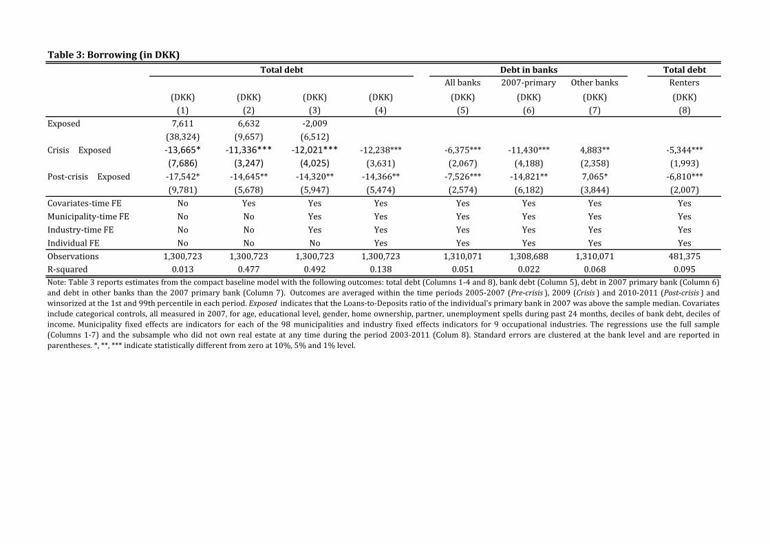
Table 3: Borrowing (in DKK)Total debt

All banks 2007-primary Other banks Renters(DKK) (DKK) (DKK) (DKK) (DKK) (DKK) (DKK) (DKK)

(1) (2) (3) (4) (5) (6) (7) (8)Exposed 7,611 6,632 -2,009

(38,324) (9,657) (6,512)Crisis × Exposed -13,665* -11,336*** -12,021*** -12,238*** -6,375*** -11,430*** 4,883** -5,344***

(7,686) (3,247) (4,025) (3,631) (2,067) (4,188) (2,358) (1,993)Post-crisis × Exposed -17,542* -14,645** -14,320** -14,366** -7,526*** -14,821** 7,065* -6,810***

(9,781) (5,678) (5,947) (5,474) (2,574) (6,182) (3,844) (2,007)Covariates-time FE No Yes Yes Yes Yes Yes Yes YesMunicipality-time FE No No Yes Yes Yes Yes Yes YesIndustry-time FE No No Yes Yes Yes Yes Yes YesIndividual FE No No No Yes Yes Yes Yes YesObservations 1,300,723 1,300,723 1,300,723 1,300,723 1,310,071 1,308,688 1,310,071 481,375R-squared 0.013 0.477 0.492 0.138 0.051 0.022 0.068 0.095

Total debt Debt in banks

Note: Table 3 reports estimates from the compact baseline model with the following outcomes: total debt (Columns 1-4 and 8), bank debt (Column 5), debt in 2007 primary bank (Column 6)and debt in other banks than the 2007 primary bank (Column 7). Outcomes are averaged within the time periods 2005-2007 (Pre-crisis ), 2009 (Crisis ) and 2010-2011 (Post-crisis ) andwinsorized at the 1st and 99th percentile in each period. Exposed indicates that the Loans-to-Deposits ratio of the individual's primary bank in 2007 was above the sample median. Covariatesinclude categorical controls, all measured in 2007, for age, educational level, gender, home ownership, partner, unemployment spells during past 24 months, deciles of bank debt, deciles ofincome. Municipality fixed effects are indicators for each of the 98 municipalities and industry fixed effects indicators for 9 occupational industries. The regressions use the full sample(Columns 1-7) and the subsample who did not own real estate at any time during the period 2003-2011 (Colum 8). Standard errors are clustered at the bank level and are reported inparentheses. *, **, *** indicate statistically different from zero at 10%, 5% and 1% level.

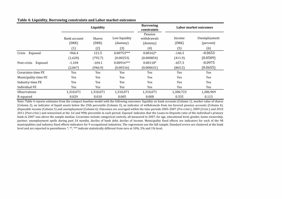
Table 4: Liquidity, Borrowing constraints and Labor market outcomesBorrowing constraints

Bank account Shares Low liquidity Pension

withdrawals Income Unemployment(DKK) (DKK) (dummy) (dummy) (DKK) (percent)

(1) (2) (3) (4) (5) (6)Crisis × Exposed -966.4 121.5 0.00753*** 0.00162* -146.3 -0.0653

(1,620) (792.7) (0.00253) (0.000854) (411.9) (0.0509)Post-crisis × Exposed -1,104 -104.1 0.00916*** 0.00118* -657.3 -0.0975

(2,067) (946.9) (0.00316) (0.000631) (865.5) (0.0655)Covariates-time FE Yes Yes Yes Yes Yes YesMunicipality-time FE Yes Yes Yes Yes Yes YesIndustry-time FE Yes Yes Yes Yes Yes YesIndividual FE Yes Yes Yes Yes Yes YesObservations 1,310,071 1,310,071 1,310,071 1,310,071 1,300,723 1,286,969R-squared 0.029 0.010 0.005 0.008 0.335 0.113

Liquidity Labor market outcomes

Note: Table 4 reports estimates from the compact baseline model with the following outcomes: liquidity on bank accounts (Column 1), market value of shares(Column 2), an indicator of liquid assets below the 25th percentile (Column 3), an indicator of withdrawals from tax favored pension accounts (Column 4),disposable income (Column 5) and unemployment (Column 6). Outcomes are averaged within the time periods 2005-2007 (Pre-crisis ), 2009 (Crisis ) and 2010-2011 (Post-crisis ) and winsorized at the 1st and 99th percentile in each period. Exposed indicates that the Loans-to-Deposits ratio of the individual's primarybank in 2007 was above the sample median. Covariates include categorical controls, all measured in 2007, for age, educational level, gender, home ownership,partner, unemployment spells during past 24 months, deciles of bank debt, deciles of income. Municipality fixed effects are indicators for each of the 98municipalities and industry fixed effects indicators for 9 occupational industries. The regressions use the full sample. Standard errors are clustered at the banklevel and are reported in parentheses. *, **, *** indicate statistically different from zero at 10%, 5% and 1% level.

Table 5: Consumption

Incl stock-owners

Excl stock-owners Renters Δ Total debt

Δ Cumm. Spending

Owns at least one car

Owns multiple cars

(DKK) (DKK) (DKK) (1st stage) (2nd stage) (dummy) (dummy)(1) (2) (3) (4) (5) (6) (7)

Crisis × Exposed -8,766*** -8,568*** -2,230** -0.00307*** -0.00142**(3,168) (2,945) (862.9) (0.000832) (0.000559)

Post-crisis × Exposed -1,548 -1,213 -1,027 -0.00277*** -0.00158**(1,954) (1,539) (865.5) (0.000903) (0.000743)

Exposed -11,577***(2,724)

Δ Debt (Instrumented) 0.984**(0.406)

Covariates-time FE Yes Yes Yes Yes Yes Yes YesMunicipality-time FE Yes Yes Yes Yes Yes Yes YesIndustry-time FE Yes Yes Yes Yes Yes Yes YesIndividual FE Yes Yes Yes No No Yes YesObservations 1,300,723 1,009,729 481,375 355,641 355,641 1,310,071 1,310,071

R-squared 0.060 0.065 0.072 0.030 0.018 0.012

Imputed spending CarsIV estimates

Note: Table 5 reports estimates from the compact baseline model with individual-level outcomes: imputed spending (Columns 1-3), an indicator of owning a car (Column6), an indicator of owning more than one car (Column 7). These outcomes are averaged within the time periods 2005-2007 (Pre-crisis ), 2009 (Crisis ) and 2010-2011(Post-crisis ) and winsorized at the 1st and 99th percentile in each time period. Table 5 also reports estimates from an instrumental variables estimation: in the first-stage, the outcome is the change in total debt between end-of 2007 and end-of 2011 (Column 4) and in the second stage the outcome is the change in imputed spendingbetween 2006-2007 and 2008-2009 (Column 5). Exposed indicates that the Loans-to-Deposits ratio of the individual's primary bank in 2007 was above the samplemedian. Covariates include categorical controls, all measured in 2007, for age, educational level, gender, home ownership, partner, unemployment spells during past 24months, deciles of bank debt, deciles of income. Municipality fixed effects are indicators for each of the 98 municipalities and industry fixed effects indicators for 9occupational industries. The regressions use the full sample (Columns 1-2 and 4-7) and the subsample who did not own real estate at any time during the period 2003-2011 (Colum 3). Standard errors are clustered at the bank level and are reported in parentheses. *, **, *** indicate statistically different from zero at 10%, 5% and 1%level.

Table 6: Real Estate

Appraisal value

Purchase of real estate

Δ Appraisal value Δ Total debt

Δ Property size

(DKK) (dummy) (DKK) (DKK) (m2)(1) (2) (3) (4) (5)

Exposed 13,332*** -3,781 0.284**(3,382) (6,828) (0.134)

Crisis × Exposed -9,486** -0.000672 -64,298*** -46,348*** -1.138***(4,189) (0.00125) (13,277) (13,600) (0.293)

Post-crisis × Exposed -10,316* -0.00131 -17,837* -18,036** -0.137(5,463) (0.00113) (10,186) (8,960) (0.207)

Covariates-time FE Yes Yes Yes Yes YesMunicipality-time FE Yes Yes Yes Yes YesIndustry-time FE Yes Yes Yes Yes YesIndividual FE Yes Yes No No NoObservations 1,300,723 1,310,071 176,737 176,737 173,073R-squared Yes Yes 0.255 0.203 0.017

Outcomes conditional on purchase

Note: Table 5 reports estimates from the compact baseline model with individual-level outcomes: total appraisal value of real estate(Column 1) and an indicator of purchasing real estate (Column 2). These outcomes are averaged within the time periods 2005-2007(Pre-crisis ), 2009 (Crisis ) and 2010-2011 (Post-crisis ) and winsorized at the 1st and 99th percentile. The regressions use the fullsample of individual-period observations. Table 5 also reports estimates from a modified model with individual-level outcomes: thechange in the total appraisal value of real estate (Column 3), the change in total debt (Column 4) and the change in the habitable surfaceof real estate (Column 5). These outcomes are not averaged within periods. The regressions use the sample of individual-yearobservations where a real estate purchase takes place. Exposed indicates that the Loans-to-Deposits ratio of the individual's primarybank in 2007 was above the sample median. Covariates include categorical controls, all measured in 2007, for age, educational level,gender, home ownership, partner, unemployment spells during past 24 months, deciles of bank debt, deciles of income. Municipalityfixed effects are indicators for each of the 98 municipalities and industry fixed effects indicators for 9 occupational industries. Standarderrors are clustered at the bank level and are reported in parentheses. *, **, *** indicate statistically different from zero at 10%, 5% and1% level.

Figure 1: Aggregate consumption and bank credit

Source: MFI Statistics from Danmarks Nationalbank and National Accounts from Statistics Denmark

Figure 2: Private consumption and Imputed spending

Source: MFI Statistics from Danmarks Nationalbank and National Accounts from Statistics Denmark

Note: Figure 1 shows the evolution of private consumption and the change in bank credit to households in Denmarkover the period 2003Q1-2012Q4 in real 2010-DKK billion.

Note: Figure 2 shows the evolution of private consumption from national accounts and imputed spendingaggregated to the population level over the period 2003-2011 in current DKK billion.

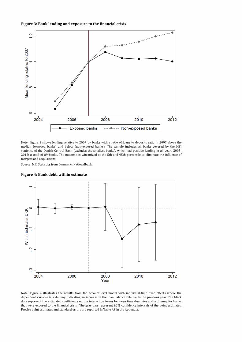
Figure 3: Bank lending and exposure to the financial crisis


Figure 4: Bank debt, within estimate

Note: Figure 3 shows lending relative to 2007 by banks with a ratio of loans to deposits ratio in 2007 above themedian (exposed banks) and below (non-exposed banks). The sample includes all banks covered by the MFIstatistics of the Danish Central Bank (excludes the smallest banks), which had positive lending in all years 2005-2012: a total of 89 banks. The outcome is winsorized at the 5th and 95th percentile to eliminate the influence ofmergers and acquisitions.

Note: Figure 4 illustrates the results from the account-level model with individual-time fixed effects where thedependent variable is a dummy indicating an increase in the loan balance relative to the previous year. The blackdots represent the estimated coefficients on the interaction terms between time dummies and a dummy for banksthat were exposed to the financial crisis. The gray bars represent 95% confidence intervals of the point estimates.Precise point estimates and standard errors are reported in Table A3 in the Appendix.

Figure 5: Total debt, difference-in-difference estimate (in DKK)

Figure 6: Effective interest rate, difference-in-difference estimate (in percentage points)

Note: Figure 5 illustrates the results from the baseline model where the dependent variable is total debt. The blackdots represent the estimated coefficients on the interaction terms between time dummies and a dummy forindividuals whose primary bank in 2007 was exposed to the financial crisis. The gray bars represent 95%confidence intervals of the point estimates. The model includes individual characteristics, industry dummies andmunicipality dummies, all measured in 2007 and interacted with a full set of time dummies, as well as individualfixed effects. Precise point estimates and standard errors are reported in Table A3 in the Appendix.

Note: Figure 6 illustrates the results from the baseline model where the dependent variable is the effective interestrate as defined in the main text. The black dots represent the estimated coefficients on the interaction termsbetween time dummies and a dummy for individuals whose primary bank in 2007 was exposed to the financialcrisis. The gray bars represent 95% confidence intervals of the point estimates. The model includes individualcharacteristics, industry dummies and municipality dummies, all measured in 2007 and interacted with a full set oftime dummies, as well as individual fixed effects. Precise point estimates and standard errors are reported in TableA3 in the Appendix.

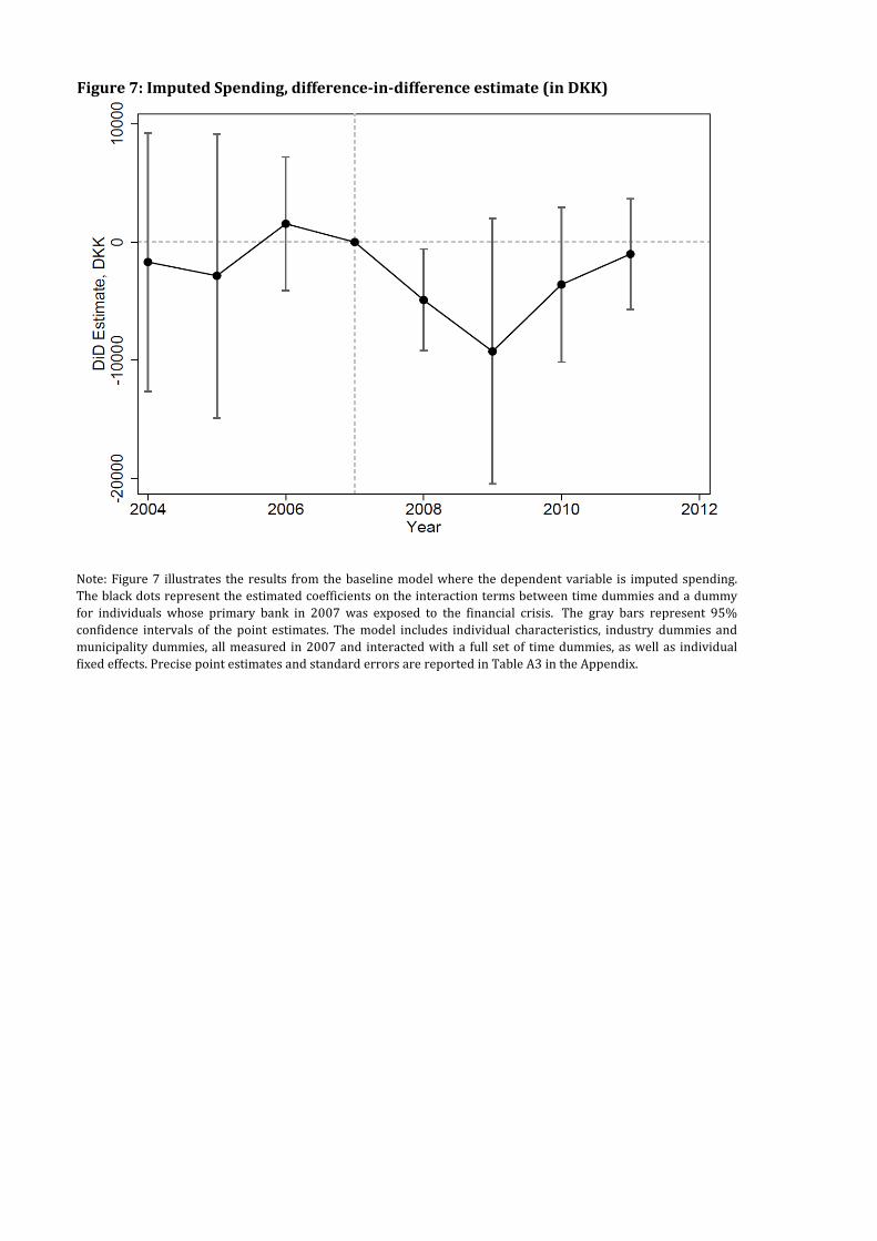
Figure 7: Imputed Spending, difference-in-difference estimate (in DKK)

Note: Figure 7 illustrates the results from the baseline model where the dependent variable is imputed spending.The black dots represent the estimated coefficients on the interaction terms between time dummies and a dummyfor individuals whose primary bank in 2007 was exposed to the financial crisis. The gray bars represent 95%confidence intervals of the point estimates. The model includes individual characteristics, industry dummies andmunicipality dummies, all measured in 2007 and interacted with a full set of time dummies, as well as individualfixed effects. Precise point estimates and standard errors are reported in Table A3 in the Appendix.

Figure 8A: Total debt, difference-in-difference estimate by liquidity (in DKK)

Figure 8B: Imputed Spending, difference-in-difference estimate by liquidity (in DKK)

Note: Figures 8A-8B illustrate the results from the baseline model where the dependent variable is total debt andimputed spending respectively and the sample is split by liquidity in 2007. The black dots represent the estimatedcoefficients on the interaction terms between time dummies and a dummy for individuals whose primary bank in2007 was exposed to the financial crisis. The gray bars represent 95% confidence intervals of the point estimates.The model includes individual characteristics, industry dummies and municipality dummies, all measured in 2007and interacted with a full set of time dummies, as well as individual fixed effects. Precise point estimates andstandard errors are reported in Table A3 in the Appendix.

APPENDIX

Table A1: Fully dynamic versions of compact models

Col. 5 Col. 6 Col. 7 Col. 8 Col. 1 Col. 2 Col. 3 Col. 4 Col. 5 Col. 6

BanksPrimary

bank Other banksTotal

("renters") Deposits SharesLow

LiquidityPension

withdrawals IncomeUnemploy-

ment(DKK) (DKK) (DKK) (DKK) (DKK) (DKK) (dummy) (dummy) (DKK) (percent)

(1) (2) (3) (4) (5) (6) (7) (8) (9) (10)2004 × Exposed 1,656 209 1,173 -43 3,179** 1,094 -0.0046 0.0002 -679 0.2420***

(2,097) (6,492) (4,234) (3,031) (1,421) (738) (0.0068) (0.0004) (548) (0.079)2005 × Exposed 1,699 1,314 508 630 2,132* 1,083** -0.0013 -0.000845** -409 0.1778***

(1,691) (5,973) (3,597) (2,496) (1,112) (462) (0.0063) (0.0003) (615) (0.063)2006 × Exposed 1,315 1,699 -268 -11 1,413* 366.0** -0.0017 -0.0005 -319 0.0745**

(2,062) (4,989) (2,176) (2,028) (844) (183) (0.0032) (0.0005) (494) (0.033)2008 × Exposed -2,640** -3520 839.2 -3,450*** -713.7 561.2 0.00784*** 0.0015 -416 0.00116

(1,135) (2,443) (1,134) (484) (1,133) (894) (0.0023) (0.0013) (287) (0.019)2009 × Exposed -5,905* -11082 5017 -4,843*** 157.5 558.8 0.00657 0.00116 -455 0.0199

(2,995) (7,089) (3,685) (547) (1,413) (855) (0.0045) (0.0009) (672) (0.044)2010 × Exposed -6,836** -13089 6044 -6,237*** -401.7 309.6 0.00879* 0.000988 -1,112 -0.0182

(3,400) (8,563) (4,726) (747) (1,762) (934) (0.0049) (0.0007) (1,072) (0.055)2011 × Exposed -6,966** -15433 8137 -6,732*** 531.7 396.4 0.00719 0.000638 -783 -0.0206

(3,441) (9,769) (5,916) (867) (1,797) (1,107) (0.0060) (0.0006) (1,265) (0.043)Covariates-year FE Yes Yes Yes Yes Yes Yes Yes Yes Yes YesMunicipality-year FE Yes Yes Yes Yes Yes Yes Yes Yes Yes YesIndustry-year FE Yes Yes Yes Yes Yes Yes Yes Yes Yes YesIndividual FE Yes Yes Yes Yes Yes Yes Yes Yes Yes YesObservations 3,486,109 3,481,107 3,486,109 1,286,901 3,486,109 3,486,109 3,486,109 3,486,109 3,455,968 3,427,790R-squared 0.164 0.17 0.063 0.215 0.036 0.042 0.005 0.018 0.357 0.085

Table 4 - other outcomesTable 3 - debt

Note: Table A1 reports estimates from the fully dynamic baseline model with the following outcomes: bank debt (Column 1), debt in the 2007 primary bank (Column 2), debt in other banksthan the 2007 primary bank (Column 3) total debt (Column 4), liquidity on bank accounts (Column 5), market value of shares (Column 6), an indicator of liquid assets below the 25th percentile(Column 7), an indicator of withdrawals from tax favored pension accounts (Column 8), disposable income (Column 9) and unemployment (Column 10). The regressions use the full sample(Columns 1-3 and 5-10) and the subsample who did not own real estate at any time during the period 2003-2011 (Colum 4). Exposed indicates that the Loans-to-Deposits ratio of theindividual's primary bank in 2007 was above the sample median. Covariates include categorical controls, all measured in 2007, for age, educational level, gender, home ownership, partner,unemployment spells during past 24 months, deciles of bank debt, deciles of income. Municipality fixed effects are indicators for each of the 98 municipalities and industry fixed effectsindicators for 9 occupational industries. Standard errors are clustered at the bank level and are reported in parentheses. *, **, *** indicate statistically different from zero at 10%, 5% and 1%level.

Table A1 (Continued): Fully dynamic versions of compact models

Col. 2 Col. 3 Col. 6 Col. 7 Col. 1 Col. 2 Col. 3 Col. 4 Col. 5Spending

(no shares)Spending

("renters") Owns a carOwns multiple

carsAppraisal

value PurchaseΔ Appraisal

valueΔ Total

debtΔ Property

size(DKK) (DKK) (dummy) (dummy) (DKK) (dummy) (DKK) (DKK) (m2)

(1) (2) (3) (4) (5) (6) (7) (8) (9)Exposed 8,368 -946.2 0.712***

(7,945) (11,867) (0.193)2004 × Exposed -1,117 1,961 0.0009 0.0005 -5,439 0.00218 -2,393 -2,030 -0.531*

(5,128) (2,191) -0.0018 -0.0013 (5,287) (0.00242) (11,452) (12,433) (0.297)2005 × Exposed -2,761 -162 0.0017 0.0005 -3,100 0.00227 8,644 3,781 -0.713**

(5,814) (1,310) -0.0017 -0.0010 (3,908) (0.00261) (11,952) (14,631) (0.349)2006 × Exposed 965 -604 0.0017 0.0003 -937 0.00319 5,669 -12,594 -0.521**

(2,590) (1,712) -0.0012 -0.0009 (2,491) (0.00218) (9,485) (10,006) (0.243)2008 × Exposed -4595 -3,090*** -0.000438 -0.000418 -3694 0.00040 -40,425*** -29,044** -1.083***

(2,823) (1,156) (0.0007) (0.0006) (3,082) (0.00116) (13,262) (14,145) (0.316)2009 × Exposed -9,201* -2086 -0.00197* -0.00121 -11,051*** 0.00109 -59,334*** -49,183** -1.567***

(5,255) (1,583) (0.0011) (0.0008) (3,320) (0.00165) (16,747) (19,006) (0.379)2010 × Exposed -2750 -1152 -0.00201* -0.00181* -11,669*** 0.00044 -10,769 -34,029** -0.472*

(3,222) (1,516) (0.0010) (0.0009) (4,076) (0.00150) (14,673) (16,324) (0.266)2011 × Exposed -1658 -125.8 -0.00123 -0.000902 -12,277** 0.00002 -15,316 -5,602 -0.672

(2,477) (1,408) (0.0013) (0.0012) (4,895) (0.00201) (17,154) (14,143) (0.488)Covariates-year FE Yes Yes Yes Yes Yes Yes Yes Yes YesMunicipality-year FE Yes Yes Yes Yes Yes Yes Yes Yes YesIndustry-year FE Yes Yes Yes Yes Yes Yes Yes Yes YesIndividual FE Yes Yes Yes Yes Yes Yes No No NoObservations 2,707,435 1,286,901 3,486,109 3,486,109 3,455,968 3,486,109 239,763 239,763 235,275R-squared 0.035 0.094 0.026 0.0190 0.294 0.019 0.250 0.203 0.017

Table 5 - consumption Table 6 - real estate

Note: Table A1 reports estimates from the fully dynamic baseline model with the following outcomes: imputed spending (Columns 1-2), an indicator of owning car (Column 3), anindicator of owning more than one car (Column 4), total appraisal value of real estate (Column 5) an indicator of purchasing real estate (Column 6), the change in the total appraisal valueof real estate (Column 7), the change in total debt (Column 8) and the change in the habitable surface of real estate (Column 9). The regressions use the full sample (Columns 3-6), thesubsample who did not hold shares (Column 1), the subsample who did not own real estate at any time during the period 2003-2011 (Colum 2) and the subsample where a real estatepurchase took place (Columns 7-9). Exposed indicates that the Loans-to-Deposits ratio of the individual's primary bank in 2007 was above the sample median. Covariates includecategorical controls, all measured in 2007, for age, educational level, gender, home ownership, partner, unemployment spells during past 24 months, deciles of bank debt, deciles ofincome. Municipality fixed effects are indicators for each of the 98 municipalities and industry fixed effects indicators for 9 occupational industries. Standard errors are clustered at thebank level and are reported in parentheses. *, **, *** indicate statistically different from zero at 10%, 5% and 1% level.

Table A2: Main results with continuous measure of bank exposure

Total debt SpendingPension

withdrawals Owns a car Real estate(DKK) (DKK) (dummy) (dummy) (DKK)

(1) (2) (4) (5)2004 × Exposure -12,126 -10,512 0.00215** -0.000374 -21,890*

(16,062) (13,896) (0.000968) (0.00549) (12,585)2005 × Exposure -13,023 -13,346 -0.000158 0.00264 -16,189*

(16,124) (13,965) (0.00131) (0.00473) (9,206)2006 × Exposure -5,226 -1,226 0.00120 0.00317 -8,553

(10,818) (7,693) (0.00207) (0.00362) (5,775)2008 × Exposure -4,763 -14,544** 0.00692** -0.00194 -4,781

(5,646) (6,899) (0.00316) (0.00208) (7,529)2009 × Exposure -19,166* -29,487** 0.00389** -0.00609** -23,509**

(9,945) (13,529) (0.00184) (0.00271) (9,715)2010 × Exposure -28,022** -19,019 0.00448*** -0.00511 -28,079***

(11,488) (11,634) (0.00133) (0.00347) (10,525)2011 × Exposure -28,188** -15,901 0.00368*** -0.00423 -33,081***

(12,868) (10,840) (0.00134) (0.00367) (11,966)Covariates-year FE Yes Yes Yes Yes YesMunicipality-year FE Yes Yes Yes Yes YesIndustry-year FE Yes Yes Yes Yes YesIndividual FE Yes Yes Yes Yes YesObservations 3,455,968 3,455,968 3,486,109 3,486,109 3,455,968R-squared 0.209 0.033 0.018 0.026 0.294Note: Table A2 reports estimates from the fully dynamic baseline model with the following outcomes: total debt (Column 1),imputed spending (Column 2), an indicator of withdrawals from tax favored pension accounts (Column 3), an indicator ofowning a car (Column 4) and the total appraisal value of real estate (Column 5). The regressions use the full sample. Exposure indicates the Loans-to-Deposits ratio of the individual's primary bank in 2007. All outcomes and Exposure are winsorized at the1st and 99th percentile. Covariates include categorical controls, all measured in 2007, for age, educational level, gender, homeownership, partner, unemployment spells during past 24 months, deciles of bank debt, deciles of income. Municipality fixedeffects are indicators for each of the 98 municipalities and industry fixed effects indicators for 9 occupational industries.Standard errors are clustered at the bank level and are reported in parentheses. *, **, *** indicate statistically different fromzero at 10%, 5% and 1% level.

Table A3: Estimates underlying figuresFigure 4 Figure 5 Figure 6 Figure 7New loan Total debt Interest rate Spending

full sample full sample full sample full sample bottom 20% middle 60% top 20% bottom 20% middle 60% top 20%Exposed -0.00319 0.00102

(0.0678) (0.00259)2004 × Exposed 0.00471 3,572 -0.000234 -1,690 -7,578* -887.4 25,994* -1,380 -2,740 2,858

(0.0186) (4,642) (0.00289) (5,581) (4,485) (4,520) (14,578) (5,689) (5,667) (8,026)2005 × Exposed -0.00187 999 -0.00191 -2,852 -7,142 -2,569 17,587 -4,397 -2,680 -1,274

(0.0128) (5,675) (0.00221) (6,135) (4,656) (5,820) (12,902) (5,528) (6,242) (8,549)2006 × Exposed 0.00368 1,631 0.000965 1,551 -4,732 -589.1 11,913 1,231 997.7 3,504

(0.00603) (3,679) (0.00184) (2,883) (3,557) (4,019) (9,491) (4,367) (2,697) (7,179)2008 × Exposed 0.00578 -3,984** -0.000816 -4,903** -7,237*** -5,653*** 2,900 -9,836*** -5,327 7,862

(0.0579) (1,635) (0.00164) (2,197) (2,309) (1,250) (3,347) (2,667) (3,547) (8,021)2009 × Exposed -0.149** -11,936*** 0.00747** -9,253 -16,408*** -12,110*** -7,374* -13,256*** -8,203 -4,578

(0.0711) (2,041) (0.00324) (5,725) (2,876) (3,138) (4,057) (4,349) (5,630) (9,483)2010 × Exposed -0.0794 -14,902*** 0.00629* -3,592 -20,059*** -14,712*** -10,052** -4,399** -3,848 1,674

(0.0912) (2,337) (0.00331) (3,344) (5,421) (2,632) (4,527) (2,169) (3,031) (8,730)2011 × Exposed -0.0688 -12,948*** 0.00181 -1,016 -22,109*** -12,065*** -5,879 -6,164*** -1,086 7,383

(0.0935) (4,283) (0.00435) (2,392) (7,880) (3,501) (4,912) (2,318) (2,146) (7,815)Covariates-year FE - Yes Yes Yes Yes Yes Yes Yes Yes YesMunicipality-year FE - Yes Yes Yes Yes Yes Yes Yes Yes YesIndustry-year FE - Yes Yes Yes Yes Yes Yes Yes Yes YesIndividual FE - Yes No Yes Yes Yes Yes Yes Yes YesIndividual-year FE Yes No No No No No No No No NoObservations 4,631,870 3,455,968 6,514 3,455,968 661,892 2,095,013 699,063 661,892 2,095,013 699,063R-squared 0.592 0.209 0.324 0.033 0.207 0.223 0.194 0.041 0.041 0.032

Figure 8A Figure 8BTotal debt (by liquidity in 2007) Spending (by liquidity in 2007)

Note: Table A3 reports the point-estimates and standard errors underlying Figures (4)-(8). Standard errors are clustered at the bank level and are reported in parentheses. *, **, *** indicate statistically different from zero at 10%, 5% and 1% level.

Figure A1: Mean ratio of loan to deposits for exposed and non-exposed banks


Figure A2: Distribution of effective interest rates

Note: Figure A1 shows the mean ratio of loan to deposits for exposed and non-exposed banks respectively over theperiod 2005-2012

Note: Figure A2 shows the distribution of effective interest rates as defined in the main text. The distribution iscensored at 2% and 20%.

Figure A3: Evolution of effective interest rates

Figure A4: Liquid assets and withdrawals from pension accounts

Note: Figure A4 illustrates the correlation between stocks of liquid assets and the propensity to withdraw fundsfrom tax favored pension accounts. The dots indicate the share of individuals withdrawing funds from such accountsin 2009 for each decile of the liquidity distribution.

Note: Figure A3 shows the evolution of the mean effective interest rate as defined in the main text and the policymonetary interest rate over the period 2004-2011.

the consumption e ects of the 2007-2008 financial crisis ... · financial crisis: evidence from...

Documents