AD-AI51 514 THE CONSTANT CURRENT STRAIN GAUGE BRIDGE(U) iAERONAUTICAL RESEARCH LABS MELBOURNE (AUSTRALIA) NE S MOODY JUL 84 ARL-STRUC-TH-385

UNCLASSIFIED F/G 9/5 N

1111- * 11.2

L L. 13 1220

JIL25

MICOCPY ESLUTONTES CARNAT11 IA BUEUOI TNAD-16-

UNCLASSIFIED

AR.L-STRUC-TM-385 AR-003 -948

I-

In

12DEPARTMENT OF DEFENCEDEFENCE SCIENCE AND TECHNOLOGY ORGANISATION

AERONAUTICAL RESEARCH LABORATORIES

MELBOURNE, VICTORIA

Structures Technical m-emorandum 385

THE CONSTANT CURRENT STRAIN GAUGE BRIDGE

E. S. HODY

Approved f or Public Release

C-,~MA I ~ g5

i.. -49

(C) C0120MM3LTE OF AUSTRlALIA 1984

COPY No JULY 194j

AR -0 03-9 48

DEPARTMN1 OF DEFENCE

DEFENCE SCIENCE AND TECILOCY ORGANISATION

AERONAUTI CAL RESEARCH 1A33O.ATORXES

Structures Technical Memorandum 385

THE CONSTANT CURRENT STRAIN GAUGE BRIDGE

by

E.S. MOODY

SUMMARY

A simplified analysis is used to developexpressions for the output of the commonly used strain gaugebridge configurations with Constant Current excitation.Expressions for initial offset compensation, shunt calibrationand the influence of lead resistance are developed. Considerationis given to some means for error correction.

COMOENWEALTHO AUSTRALIA 8..4

P'Z-.AL ADDRESS: Director, Aeronautical Research Laboratnres,8

P.O.~~~~~ ~ ~ ~ ~ ~ bo 431 ebune.otra 00,Asrla

r ONTENT S

PAGE NO.

1. INTRODUCTION1

2. BRIDGE FORMULAE1

3. THE INITIAL OFFSET3

4. OFFSET COMPENSATION AND SHUNT CALIBRATION6

5. SHUNT CALIBRATION AND LEAD RESISTANCE 6

6. OFFSET COMPENSATION AND LEAD RESISTANCE 7 -

7. THE 7-WIRE BRIDGE 8

8. CONCLUSION9

REFERENCES

APPENDIX

APPENDIX 1

APPENDIX 2

TABLES

GRAPH

FIGURES

DISTRIBUTION LISTI

%DOCUMENT CONTROL DATA-NTIS GRA&IDTIC TABUnanrnouinced ElJustificatio -

By-Distribution/

Availability Codes

Avail and/orWo

Dist Special

1. INTRODUCTION

°0ii the early electrical strain gauge bridge circuits employed

constant voltage sources for bridge excitation. The technqiues developed

for the classical direct-current and alternating-current component- -

measuring bridges were transferred to the strain gauge bridges with only 9minor modification.

With the introduction of the semi-conductor strain gauges the

advantages to be gained by the use of constant current bridge excitation

became apparent. However, the difficulties associated with the construct-

ion of suitable constant current circuitry inhibited its introduction on

a large scale until the mid 1970's. The availability of inexpensive high-/

gain, integrated circuit amplifiers has simplified the task of producing

practical constant current supplies, and by the end of 1979 extensive use

of this form of excitation was being made in these Laboratories.

4)While the use of constant current sources does provide a bridge

of enhanced stability, the network shares some of the problems of the

constant voltage circuit and introduces a few of its own. In this paper

an attempt has been made to present some of the formulae for the constant

current bridge, to investigate the effects of lead resistance and to

examine, for the simplest bridge, the influence of initial offset compen-

sation (initial balance) on the sensitivity of the bridge to strain and

on the bridge configurations to be used.-

2. BRIDGE FORMULAE

The expression for the output voltage (Vo ) of the general Wheat-

stone network in Fig. 1, is established in Appendix 1. This development _.

is for a simple, essentially equal-element bridge in which only small

changes in resistance take place. However, the procedure used is quite

general and appropriate for elements of any value. An infinite input-

impedance detector is assumed.

The expression for the bridge output voltage is:

S

* " ''--.-.--- .- ,' ' - ".---'-. - -. - . rr-

-.rm . i . .r '-~-c , r r - . . s*-. 'c - .-s s-- .y--.7 -T o

[21

[ a(l+d) + d ] - [ b(1+c) + c ]V = x [I.R.]o ~~4 + a + b + c + d - .. ,

Where I is the constant current injected into the circuit at node 1 and

R is the initial, undisturbed value of each bridge element, usually

referred to as the bridge resistance, and a,b,c and d are small fractional

departures of each element from the value R. From the above expression,

by selecting appropriate values for a,b,c and d, the formulae for the ".

output voltages of the commonly used strain gauge configurations can be

obtained. These formulae, together with the corresponding expressions

for the equivalent constant voltage circuits are set out in Table 1.

-SThere are several points to be noted about the constant current

formulae: -

[a] The output voltage, Vo, is directly proportional to bridge 0

resistance.

[b) For the three possible two-active-element configurations

the output voltage is the same.

[c] Comparison of constant current and constant voltage expressions

shows the improvement in linearity achieved with constant

current. However, the nonlinear term is present in both

bridges and, as Troke(2) has pointed out, this nonlinearity

must be taken into account in all cases where shunt calibration

techniques are used to establish strain sensitivity.

[d] Where all elements of the bridge are equally active, or where

two adjacent elements across the supply are equally active

(the changes in both cases being additive) the formulae for

constant voltage are direct equivalents of the formulae for 0

constant current.

• .S ..

[3]

The appearance of the bridge resistance in the expression for

the output voltage is of concern to users of constant current bridges.

Fortunately, the change in this term with temperature and with time is

small, and its influence on bridge output voltage is generally negligible.

In a good quality strain gauge bridge R may change by 0.04 ohms in 120

for 100 degrees Celsius change in temperature. This will change the

output by about 0.03% for 100 degrees temperature change. It is of

some interest to note that the expression for the short-circuit output

current of the constant current bridge is independent of bridge resistance.

At the present time, current-sensitive detectors are out of

favour for strain gauge bridges and, in any case, would need to be

located at the bridge to avoid lead resistance effects. Systems providing

signal conversion at the gauge site are currently receiving attention,

and perhaps current detectors may be restored to favour in the future.

3. THE INITIAL OFFSET

Strain gauge bridges, particularly those used in structural

testing as distinct from those in load cells, are rarely perfectly '.-

balanced, and a significant offset voltage will be present in the output.

Before mini and microcomputers were introduced to strain gauge instrument-

ation an initial balancing circuit was considered an essential feature

of the complete bridge network.

There were two major drawbacks to the initial balance circuit.

Firstly, even when large and costly components were used, random jumps

in the initial output could not be completely eliminated. Secondly, this

circuit places shunting resistances of indeterminate value across two

adjacent arms of the bridge thereby upsetting the thermal symmetry and,

for a four-active-element bridge, reducing the bridge's sensitivity to

strain by an incalculable amount.

The computer can provide automatic correction for any initial

offset, and with the very long scale length of modern voltmeter-detectors,

minimization of initial offsets is only rarely required. When some adjustment .

is necessary the degree of precision required is low and may be achieved by

shunting one ele.nent of the bridge with a stable, fixed resistor. The value

of resistance to be used can be determined most readily using a decade

resistance box.

j41

It should be clear that a shunt across an active element will

reduce the sensitivity of the effective total element to any strain

induced resistance change, but it may not be apparent that any shunting

of a ratio-arm to achieve initial offset compensation may also bring

about significant change in sensitivity to strain. Examination of

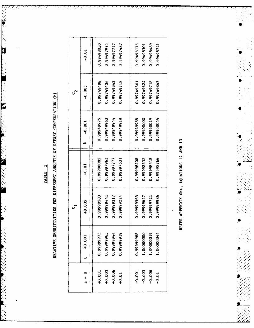
equations (8) to (11) in Appendix 1, and the sensitivity ratios set ..I .out in Table 2, will show that the influence of the initial offset

compensation on the bridge output varies with the compensation used.

It can also be seen that for the worst case the loss of sensitivity is

0.5 percent. For purposes of illustration, it has been assumed that

the bridge of Fig. 1 has three equal elements A, C and D and that element

B is either larger of smaller.

For the above conditions there are two options available for -

initial offset compensation:-

[1] Where B is larger than the other elements, element D may

be increased or element C decreased. --

[2] Where B is smaller than the other elements, element D may

be reduced or element C increased.

In equations (8) and (11), where offset compensation involves

adjustment to element C, the initial fractional offset value 'b' does

not appear in the numerator, and appears only as 'b2', a very small number,

in the denominator. However, in equations (9) and (10) where offset

compensation is achieved by making adjustments to element D the fractional

offset value appears in the numerator, and in the denominator it is

doubled. As expected, the results in Table 2 show that when equations . -

(8) and (II) apply, the change in sensitivity are negligible, but can be

as high as 0.5 percent when equations (9) and (10) apply. If sensitivity

changes of this magnitude cannot be tolerated, adjustments for both signs . -

of offset in element B must be made in element C, either a shunt across

it or a small resistance in series with it.

Clearly where the strain sensitivity is determined only after

the offset adjustments have been made the above problem does not arise.

Unfortunately, calibration after initial offset compensation is not always

possible, and if accuracy is paramount, a calculation of the change should

[51

be made. In a practical bridge elements A and B may be equal, and C

and D equal to one another but not equal to A and B. Setting nominal

values of elements A and B equal to R1 and C and D equal to R, and then

substituting in equation 1 of Appendix 1, expressions for bridge output

voltage for compensated and uncompensated bridges can be determined.

Using the symbol 6 for those small fractional changes from the mean

value resulting from strain on the element and setting a = +6,

b = +b, c = -b/l+b, d -

IR R6 .V = b(R1 - R) + b.R1

. ...

2(R + R1) + 6R + 1 + b--

1

For a = +6, b = -b, c = J, d = -b:- 0

IR R6(l - b)V ... 1 (3) - . -6 2(R + R) + 6R -b(R + R1 ) A

When the bridge has no offset compensation the output for a = 6, b +b,

c , d 6 is:-I I . .0 .

6-b bV-1o - IRIR + I ..(4) • .-61 1 R (2 + 6+b) +2R RI (2 +b) +2R ----- ,"

For a = 6, b = -b, c = €, d =

V 1 = IR1R .. (5) 2- i ..R (2+ -b)+2R R (2-b)+2Rj

5-S"

With these four equations and a knowledge of the resistance in the bridge

prior to compensation an accurate assessment of the effect of compensation

on strain sensitivity can be reached.

01

[6]

4. OFFSET COMPENSATION AND SHU'T CALIBRATION

If the signal from shunt calibration is to be the basis for

strain calculations and not simply a check on system sensitivity the ...

element, or for bidirectional calibration, elements shunted should

not include the element used for initial offset compensation. For

a bridge with a single active branch containing one or two active

elements both offset compensation and uni-directional shunt calibration

may be performed across the ratio arms thereby avoiding the problems

introduced by lead resistance. In the general case, however, initial

offset compensation should be applied in one branch and shunt

calibration in the other.

5. SHUNT CALIBRATION AND LEAD RESISTANCE .

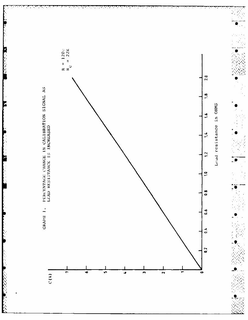
The errors arising from the presence of significant lead

resistance, or from lead resistance change, are well known, and

demonstrated in Graph 1. --

A general expression for the output voltage produced by

shunting one element of a constant current bridge with a resistance

RCAL , in the presence of lead resistance, RZ, as shown in Fig. 2. is

developed in Appendix 2. This output voltage is:-

I (R2 + 4Rj (R + R)]-

OCI 4[ L + 2Rz + RCAL 0

When Re is set to zero in this expression it reduces to:-

1R2

OC2= .. (7)2 4 [ AL+ A I

Equations (6) and (7) can be combined to provide an expression for

the percentage change in the shunt calibration signal with change in

lead resistance.

.S ,

F0

[777

VOCI 1, 100 4 [R2 + dRL(R R)H + 1 100

V R 2 [ " + 2R + RA 1LOC2 j 4 CAL

This can be reduced to an expression independent of the value of RC

by discarding 2Re from the denominator to give:-

L 4Re(R + Rj)V 1 100

V oc2 R

While the assumption of symmetrical lead resistance, and lead resistance

change is not always valid the approximation is sufficiently good for

all practical installations.

In Graph 1, the percentage change in calibrate signal, C, is

plotted as a function of R over a range of values from 0.2 to 2.0 chms.

From this graph it is clear that lead resistance values should not

exceed 0.1 ohms if this effect on calibrate signal is to be ignored.

It would be very difficult to hold lead resistance to this low value,

and a reasonable conclusion from Graph 1 is that shunt calibration is

best avoided in 4-wire bridges; if shunt calibration is unavoidable,

a 6-wire bridge should be used. Only the 6-wire circuit, or a 7-wire

arrangement for bi-directional calibration, will completely eliminate

these lead effects. Fortunately, with the constant current supply, wire

diameters can be reduced to compensate for the additional wires. As

a last resort, the resistance of the lead can be estimated and a correction

applied.

6. OFFSET COMPENSATION AN) LEAD RESISTANCE

The formulae developed for the shunt calibrate circuit can

also be applied to the initial offset compensator where it is being

shunted across a remote element. In this case changes in the lead

resistance will induce small changes in the offset correction and appear

as drift in the residual initial output voltage. In this case the

calculated percentage change in the calibrate signal becomes the

[8]

percentage change in the compensating voltage. If unknown, the size of

the initial offset, and hence the size of the compensating signal can

be approximated from a knowledge of the compensating resistor. The

* percentage change for lead resistance change is applied to the

compensating signal, and clearly the larger the initial offset the

larger will be the drift from lead resistance.

For the single active branch bridge, with compensation across

or in series with one of the ratio arms, lead effects on compensation

can be ignored. Where the 4 elements of the bridge are installed at

the measuring site series offset compensation would require the install-

ation of small resistors adjacent to the gauge and as close to it as

possible. The series resistor cannot be mounted remotely because this

would introduce significant amounts of temperature sensitive copper lead

wire into one bridge element and destroy the thermal stability of the

bridge. If the gauge is not accessible, and in most structural testing

applications it will not be, one arm of the bridge will require to be

shunted when offset compensation is essential.

To minimize lead effects for remote shunt offset compensation

this shunt must be provided with separate leads as for the calibrating

shunt. This requirement could increase the total number of leads to 8

or, for bi-directional calibration, 9 wires.

7. THE 7-WIRE BRIDGE

Bi-directional shunt calibration is very rarely required for

gauge systems used in structural testing. Therefore, the maximum number

of wires required for a bridge in this application will be eight, four

for bridge supply and signal output, two for the shunt calibrate resistor

and two for an offset compensator if it is needed..

In those situations where the shunt calibrate resistor and the

shunt compensator are applied across adjacent elements in an 8-wire2

configuration, or where the requirements can be adapted to place these*

shunts across adjacent elements, one lead wire may be shared and the .-

bridge reduced to a seven-wire circuit.

[9) 0

In Appendix 3 the equivalence of the 8-wire and 7-wire bridges

is studied, and it is shown that errors, if any, resulting from the

discarding of one lead wire is negligible. The shunt calibrate signal

is the same for both 7-wire and 8-wire bridges. However, the influence

of offset compensation on bridge sensitivity should be kept in mind when

trying to bring the shunting resistors to adjacent elements.

8. CONCLUSION

Constant current excitation provides a stable strain gauge

system but a six-wire or eight-wire bridge must be used if shunt

calibration procedures are employed and a high level of accuracy is

required. The large number of wires per bridge can aggravate installation

and trouble-shooting problems.

An alternative to the multi-wire bridge is the placing of

bridge conditioning and detecting circuits so close to the gauge measuring

sites that lead resistance can be neglected. From Graph 1, it can be seen -

that for a 4-wire constant current bridge with shunt calibration the lead

resistance must be less than 0.1 ohms if corrections to the strain-

equivalent-of-calibrate signal are not to be made. Four metres of 20 SWG

solid copper wire, or 2.4 metres of 14/0.193 mm stranded hook-up wire

will produce a resistance of 0.1 ohms. This is a relatively short length

of wire in most gauge installations, and if the wires must be longer,

either 6 wires should be used or a computed correction applied.

. . . ......

- -

' .i ...-

REFERENCES

0

[1] TROKE, Robert W. "Improving Strain Measurement Accuracy

When Using Shunt Calibrations".

Experimental Mechanics, pp. 397-400,

October 1976.

APPENDIX 1

A common procedure for bridge analysis will be used throughout

these Appendices and it is set out in some detail here. The general

equations for the network of Fig. 1 are:-

1+1 I1 2

Ij [R ~ + B 1 RC I RD

WNV 0 =11 R A 1 2 Rc C

whence,

_T.

[R LA (R:C+ RD,) -RC(R A +RB)]

RA+RB + Rc + RD

RA RD RC R B

LA+ RB+ RC D

If we assume a nominally equal-element bridge in which each element

differs from the nominal value by only a small amount, and this difference

is expressed as a fraction of the nominal value, equation (1) can be

written:-

fROl+ a) R (1 +d) -O R +c0 R(1+ b)]IV =

oR(4 +a+ b+ c +d)

which in turn reduces to:-

IR [ a(1+ d) + d] [b~l+ c) + c]0 +V~~

0S

The fundamental strain gauge equation is:-

6 = GF.c

Where GF = Gauge Factor, e = Strain and 6 = resulting fractional change

in resistance.

By substituting appropriate values for a,b,c and d, Equation

(2) yields the expressions for constant current bridge output contained

in Table 1 as follows:-

1. For 2 adjacent elements with equal and opposite strain

values:a = 6, b = -6, c 0, d 0.

Equation 2 becomes:

IR [6 - (-6)]

o 4+6-6 ..

IR6_ .. (3) .

2

2. For corresponding elements in the two branches subjected

to equal strains of opposite sign: a = 6, c = -6, b 0, d = 0.

Equation 2 becomes:

IR [6 - (-6)]

0 4+6-6

IR6- - .(4)

2

3. For equal strains in alternate elements: a = 6, d 6,

b = 0, c - 0.

Equation 2 becomes:

IR [6 (1 + 6) + 61

0 42,.'.i @ o 4 + 26 -'-'-

1R6

2 . ..(5) 771

r......~ ~~ ~~~~ -°- . .rr f-rrr v -~.

A1.3

4. For a single active element: a 6, b = 0, c 0, d 0.

Equation 2 becomes:

IR [6 (1 + *04+v° = ~4 + 6 -:---"

IR6- - .6

4+6

5. For equal additive strains in the four elements:

a - 6, b -6, c - -6, d = 6.

Equation 2 becomes:

IR [ [6(1 + 6) + 6] - [-6(1 -6) -6] ]V4+6-6-6+6 •

= IR6 ..(7)

Equation 2 may be used to investigate changes in element strain

sensitivity with changes in initial offset compensation, but first it

is necessary to establish values for c or d which will compensate for

particular initial values of b,

1. Let b have the initial value +b, and let a-0, d=0. The - -

bridge can now be balanced by shunting element C until

c = -b/l+b. With this value substituted in Equation 2 0

it becomes:

IR b (1 -- b b.-"0 b . "

4 + b -l-b-1+b

and the bridge is balanced. .

2. With the same conditions as in 1 above the offset compensation

could have been achieved by placing a small series resistance

in element D to make d-+b. Equation 2 then becomes: •

A1.4

IR [+b - b]V 4+b+b

and the bridge is balanced. 0

3. Let b have the initial value -b, and let a=0, c-0. The

bridge can now be balanced by shunting element D until

d=-b, or by increasing element C with series resistance

until c = b/1-b. That compensation is achieved with d=-b

should be obvious. When c - b/i-b, equation 2 becomes:

IR -- b(1 + )+-

V o 4 -b + b i.?1-b

When element A is strained without initial offset compensation the output

from the bridge will be the algebraic sum of offset output plus strain

output. Assuming c=O, d=O, a=6, b=+b, equation 2 can be used to derive

an expression for the output produced by strain alone. S

±6+b

and similarily when b =-b,

VR+b Ib - -4 6- bj 4- b

For the two conditions of initial offset considered, namely 0

b ±b, four expressions for the output from an initially balanced bridge ...

can be derived, one for each of the methods used to give initial offset

compensation. They are as follows:

1. For a -±,b +b, c -b/1+b, d = . Equation 2 gives:

F ~1+b 1b

± IR6 1:6

2. If initial offset compensation had been achieved for 1 above

by adding resistance to element D insteady of shunting element

C the values would be a t 6, b -+b, c = ,d +b, and

equation 2 gives:

V 6 IR[± 1 b :b ]

±IR6 (1 + b)

4 ± 6 + 2b

3. For a ±6, b -- b, c -0, d -- b, initial offset compensation

is achieved by shunting element D and equation 2 gives:

V 6 - IR - -

±IRS (1 - b)

4 ± -2b

4. For a -±6, b =-b, c -b/i-b, d 4,initial offset compensation

is achieved by adding resistance to element C instead of shunting

element D. Equation 2 now gives:

1b 1bV - IR

4 6 b +

1-b

- ±1R6 .(1

4± 1f-b

A1.6

To illustrate the change in sensitivity with initial offset

compensation the ratio V6/V61 can be calculated. This has been done -

for equations (8) and (10) using the expressions:

V6 (4± 6 + b) (4 + b)

V61 2(2 + b) (4 6+.j) b. 2

for a - ±6 , b -+b, c- -b/l+b, d = *; and

V6 (4 6 -b) (4 -b) (1- b)

V6 1 2(2 - b) (4 ± 6 - 2 b) 2 ."1"

.0

for a = ±6, b = -b, c = *, d = -b. The results for several values of

fractional resistance change in element RA , a = 6 and several values of .-.

the initial offset b for which compensation has been applied are

tabulated in Table 2. Only the single-active-gauge bridge is examined -

because this is the most likely circuit to require initial offset

adjustment, and because the equations describing this circuit are

reasonably manageable.

0

-9 .

-0 -.

APPENDIX 2

An expression for the output voltage from a simple bridge 0

when one element is shunted by a fixed resistor is developed. The

analysis is appropriate for the shunt calibration resistor, RCL or

for the shunt initial offset compensator, R Lead resistances

are included and the justifiable assumption is made that all lead

resistances are equal. The circuit is given in Fig. 2.

In Fig. 3a lead resistances which do not influence the output

voltage have been removed and the layout changed to highlight the

transformation to be made in order to arrive at the circuit of Fig. 3b.

For the general case where the elements are RA RB, R and R D ,

the expressions for circuit currents and voltages are cumbersome. ,0

However, by using the fractional forms R(l+a), R(l+b) etc. together

with single symbols to represent complex expressions, the analysis is

manageable.

From Fig. 3b by inspection:

i R(l+a)(2+c+d) CAL R(1+a)(l+b) 1-I -I CAL ] R + = L Rt+ R CAL + ... ........

4 +a+b+c+d1 4'L 4+a+b+c+d

By setting 4 + a + b + c + d = Z this expression reduces to:

I [ R.7 + R(l+a)(2+c+d) ]

CA = [( 2Ri + RAL) + R(l+a)(l+b) + R(l+a)(+c+d)

C0

Set the coefficient to I equal to Y, and the expression becomes:

I '~... (1

CAL

From Fig. 3a by inspection:

12 R(1+c) + R(1+d) ] ( I - I - ] R(1+a) + [ I - I R(l+b).2CAL 12 12

D 0

A2.2

Substituting for ICAL and using Z this expression can be rearranged

to give I2:

12 - [ 2+a+b- Y(l+a) ] . ..(2)

An expression for bridge output voltage can also be obtained by

inspection of Fig. 3a:

V 2R(l+d) - (I I-12 R(l+b) + ICAL R]

By subsitituting the values for ICAL and 12 given in equations

1 and 2, and letting R A = RC =R C =R such that a b c d

this expression reduces to:

21R (2 - Y)V- I[R + YR£]. ..(3)

To illustrate the effects of lead resistance on the shunt

calibrate signal, or on the offset compensating voltage, equation 3

can be written:

I[R 2 + 4Rz(R + Rj)]

V OC ..(4)4[3R/4 + 2Rt + RCAL]

The reference value occurs when R= 0. The equation then becomes:

1R2

OC2 (5)4[3R/4 + RC I.

Equations 4 and 5 can be combined to given an expression for

the percentage change in shunt signal as the lead resistance increases

from zero:

S~iil.:

A2.3

[R2 + 4Re (R+Rz)] [3R/4 + RC L ] 10

L R2 [3R/4 + 2R + RCAL ]

The percentages are shown graphically for lead resistance values up

to 2 ohms in Graph 1.

Note that in equation 6, 2RC is very much smaller than RCA"

and it should be a reasonable approximation to discard the lead

resistance from the denominator. If this is done the expression

becomes independent of R CAL The degree of dependence of the percentage

change in the shunt calibrate signal on RCAL is demonstrated using

equation 6 for two values of RCAL. The values obtaived are set out

in Table 3. When 2R is discarded from equation 6 the expression for =0

percentage change can be reduced to:

C z + 1 .00 .. (7) •

R2-

." .-S

0.-

APPENDIX 3

The circuits to be compared are in Fig. 4a, the complete

8-wire bridge, and in Fig. 4b, the shared-wire, 7-wire bridge.

When the shunt calibration circuit is open, the circuits

of Figs. 4a and 4b are identical. As well as being the condition for -"

normal operation, this is also the condition for initial offset

compensation, and for equal values of offset 'a' and lead resistance

Rt the value for RSHNT will be the same in both circuits.

For initial offset compensation it was shown earlier that

the value of the shunt, RSHNT + 2R across R must reduce the value

of this bridge element to R(l-a/l+a) which can be simplified to

R/l+a. Therefore, for both these circuits, initial offset compensation

will be achieved when:

C RSHNT + 2Rl ) R R

(RST + 2R) + R 1+a .

If R + 2R is replaced by r a simple expression relating 'a',SHNT E2

the offset, and r the offset compensation is:

or2

Ra= -

Fig. 4b shows the shared-wire, 7-wire bridge with the shunt calibrate

circuit closed. This circuit can be transformed to that of Fig. 4c,

which is of the same form as Fig. 4a, by performing a star-to-delta _0

transformation on the shunting circuit. After transformation, the

shunt calibrate circuit will have the values:

(RcAL + Rj) RtRCAL + 2 R +

STINT

(Rca + Re) R'i.e. r + CAL t R t) r2

(R sHNT + R)

A3. .2

The shunt compensation circuit will have the values:

(R + R RR + 2Rj +

SRNT (Rc + R)

i.e. r1 + (R SHNT+ Rt)Rt rj(R CAL+RPf)

and, as shown in Fig. 4c, a third component appears shunting the

output and with a value given by:

(R CAL + Rd) (R SHT + R4) + RS + R + 2R

Ri HN CAL '

The resistance of this output shunt is very high because it contains

the product of two large resistances R and R divided by theCAL SHNT

lead resistance which should never be greater than I ohm. Since it

is only in shunt with the output, it can be discarded for this

exercise.

By discarding the output shunt, Fig. 4c becomes identical in

form to Fig. 4a, and from this it can be assumed that the circuit of

Fig. 4b can be replaced by the circuit of Fig. 4a if r1 and r2 are

replaced by riand r -

To determine the maximum differences between r1 and r and

between r2 and r , the maximum value for R and R can be taken.2 CAL SHNT

as 200 000 ohms; and the minimum values can be taken as 10 000 ohms.

With R. at 1 ohm the above figures yield differences of 20.0 and 0.05.

Notice that when the difference is a maximum, the value of r is also.

a maximum and when the difference is a minimum r is also a minimum.4

For the maximum difference, the correction is one part in 10 and for4

the minimum difference, it is one part in 20 x 10 . While these small

terms are unlikely to influence the output to a significant degree,

numerical values have been determined for the four possible combinations

arising from the values selected. The values of 'a' corresponding to

A3.3

the values of RSHNT are calculated using equation (1), and the various

values are set out in Table 4.

For Fig. 4a, the following expressions can be developed: . .

I(2r 2 + R) (r1 + R) (

(2r2+R)(rl+R) + (r2 +R)[rl(2+a)+R(l+a)]

I(r2 + R)[rI(2+a) + R(l+a)] 0

(2r2 +R)(rl+R) + (r2 +R)[rl(2+a) +R(l+a)]

The output from this bridge is given by:

V II R(l+a) - 12 R

which, when the above expressions for I and I above are substituted,1 20

becomes:

IR [R(r 2 -r) +r2 a(rl+R)]

0 (2r2 +R)(r +R) + (r2 +R)[r (2+a)+R(l+a)] .

Equation (4) can be used to compare outputs from the circuits

of Figs. 4a and 4b by using r1 and r2 to calculate Vo, and then using

r' and r' to calculate V'.o

The values used for r,, r2 and r, r are shown in Table 4,

and the calculated values of V /IR are set out in Table 5. It can be

seen that the differences for corresponding conditions in the two

bridges are negligible.

e-

0'i. .-

TABLE 1.

BRIDGE OUTPUT VOLTAGE FORMULAE

Conia~tonCzonstant current Constant volta::e

-IRi V:

.1 V V =o 4+~ o +2 f

Cne active arm

v IR

V = - -.- -

o 2 0 4i

o 2 0 2+-

Twc a~ms ctiv

IT ! R' V7z~i ar-S - ti0

0 n LP r- r- L r %u-i " en c 0 00 -4

ON a, ON 0% ON 0% 0%. 0%

ON 0 ON0 0% ON 0h 0% 0000 0 0 0 0 0 0

00 00 V 00 700 e

o" 0 en I - 4 - 4 0u-I -1to C4 ' Lfn %0 Ir. w

.0 0 m% 0a% 0m 0%0%h %

ON 0 ON% 0% 0% 0% 0% ON

0000m N 000

0% Ci 0% 00% m N s

0 0% ON 0% 0Y% ON 0 0 0Ncr

*r -Lt 4 -n- m Lin LI

0l ON0% 0 0% m% 0% 0 0m% 0 0% 0, m% ON 0% a%

0Q z

-44 _- It_ _ _ _ _

T -. " 0Q CN -" 0e* 0. 0n N 1- %0 r- m

0%m 0% a% a, 0% 0% m%

+ 0% 0% 0 0% ON0 0 0 -

m~ m 000 0000 0 '

cn %0

c0C 0 0 00

TABLE 3

INFLUENCE OF LEAD RESISTANCE ON CALIBRATE SIGNAL

Refer Appendix 2, Equation (6)

[ Rt PERCENT ERROR IN SHUNT CALIBRATE SIGNAL

OHMS R - IOK 0OHMS R -200K OHMSCAL CAL

0 0 0

0.2 0.6638 0.6676

0.4 1.3297 1.3373

0.6 1.9979 2.0094

0.8 2.6681 2.6836

1.0 3.3406 3.3601

TABLE 4

REFER APPENDIX 3

R R r~ rCAL SHNT 1a 21

10K 10K 0.012 10002 10002 10003 10003

10K 200K 0.0006 10002 200002 10002.05 200022 -0

200K 10K 0.012 200002 10002 200022 10002.05

200K 200K 0.0006 200002 200002 I200003 f200003

TABLE 5

REFER APPENDIX 3

rI r 2 V /IR

10002 10002 2.97313 x 10.3

10003 10003 2.97314 x 10-3

10002 200002 2.97265 x 10- 3

10002.05 200002 2.97265 x 10-3

2-4200002 10002 1.50518 x 10-4

200022 10002.05 1.50518 x 10-4

200002 200002 1.49933 x 10-4

200003 200003 1.49933 x 1 . O-

D_ - 9

:72

~NCN

0-4

E-4I

4 1

-<

CC!

dim

R (1 a) R Rc ~l~c

Fig. 1.

70

RA RCAL RC

RDR

FIG. 2.

1CAL Re

1 -ICAL

I -I -iCAL0

FIG. 3 (a)

Delta star tra'.sfzrmation

I-ICAL

RA

PA4-RB+RC +RD

RA+RB-RC-RD

FIG. 3(b)

7 7

RA R ?:AL RSHiNT Rc R

RB =R(l--3 Ra R

FIG. 4 (a) 0

R RR:2AL RSH.:T

i0 Vo 0-ii 12

R. (ia) R

FIG. 4 (b)

(RCAL+R!) R; (S H T +R e) R~RS HNT+Rc- RCAL+RK

A R Ri

RCAL SN.

R ( 14a)R

FIG. 4 (c)

Jo0

DISTRIBUTION

AUSTRALIA 0

Department of Defence -.

Central Office

0

Chief Defence Scientist )Deputy Chief Defence Scientist )Superintendent, Science and Program Administration ) (I copy)Controller, External Relations, Projects and Analytical )

Studies -Defence Science Adviser (U.K.) (Doc Data sheet only) .Counsellor, Defence Science (U.S.A.) (Doc Data sheet only)

Defence Science Representative (Bangkok)Defence Central LibraryDocument Exchange Centre, D.I.S.B. (18 copies)Joint Intelligence Organisation .6Librarian H Block, Victoria Barracks, Melbourne

Aeronautical Research Laboratories

DirectorLibrary

Divisional File - StructuresAuthor: E.S. MoodyM.T. AdamsL. Conder

P. Ferrarotto

C. Ludowyk

Materials Research Laboratories

Director/Library

Defence Research Centre

Library

Navy Office

Navy Scientific Adviser

Directorate of Naval Ship Design

Army Office

Scientific Adviser - Army

Engineering Development Establishment, Library

Air Force Office

Air Force Scientific AdviserAircraft Research and Development Unit

Scientific Flight Group 0Library

. . /cont.

DISTRIBUTION (CONT.)

Air Force Office (cont.) 0

Technical Division Library

Director General Aircraft Engineering - Air ForceHQ Support Command [SLENGO]

Department of Defence Support 0

Government Aircraft Factories

ManagerLibrary

Department of Aviation

Library

Statutory and State Authorities and Industry

Hawker de Havilland Aust. Pty. Ltd., Bankstown, Library

Universities and Colleges

Adelaide Barr Smith Library -"

Flinders Library

Latrobe Library -'

Melbourne Engineering Library

Monash Hargrave Library 0

Newcastle Library

Sydney Engineering Library

N.S.W. Physical Sciences Library

Queensland Library *

Tasmania Engineering Library

Western Australia Library

R.M.I.T. LibraryDr H. Kowalski, Mech. & Production

Engineering

CANADA

NRCAeronautical & Mechanical Engineering Library

FRANCE

ONERA, Library

... /cont.

DISTRIBUTION (CONT.)

INDIA 0

National Aeronautical Laboratory, Information Centre

ISRAEL

Technion-Israel Institute of Technology

Professor J. Singer

JAPAN

Institute of Space and Astronautical Science, Library

NETHERLANDS

National Aerospace Laboratory [NLR], Library

NEW ZEALAND

Defence Scientific Establishment, Library

UNITED KINGDOM

Royal Aircraft Establishment

Bedford, Library -

National Engineering Laboratory, Library

Universities and Colleges

Cranfield Inst. of Technology, Library

UNITED STATES OF AMERICA

NASA Scientific and Technical Information Facility

SPARES (10 copies)

TOTAL (81 copies)

$ Si

S

0",%Pent o D~S

DOCUMENT CONT7ROL DATA

I a AR No i b Eirubtwment No 2 Dmornnit Date 3 Tusk No

AR-003-948 ARL-STRUC-TM-385 July 1984 DST 82/007

S.il 5Sincu.,try 6. No Pugma docuMl

THE CONSTANT CURRENT STRAIN GAUGE UNCLASSIFIED 32BRIDGE b sale c abstract 7 No 0e

U U1

AuthoiU) 9. Dowading Iflstructiont

E.S. MOODY

10. Corporate Auth~or pdAddrm ~11 Autwrutv (a9WVPdWd)I .. OW1 b.91cul c.wo% d.amAeronautical Research Laboratories,

PO Box 4331,*MELBOURNE, VIC. 3001

12. becondoty Dti iutt~ o If this dociflam t)

Approved f or Public Release.

Ovirmn tuirers outode snstsd lmmnations ewouic be referrd throuo ASOIS. Defnc Ivnformation Servica Broxh,Deprwmnt of Dglences CWrWbWl Park, CANBERRA ACT 250113..*. T"e doacart may be ANNOUNCED ir. Wtalogues and awareness wvtcas avalable to

No limitations.

13. b. Citation lor other purol li4 canw anisaunewrien) may be [same) urtres?',iedforl &L f 13 6.14. oic-rroors 1b. COSATi Catou

Strain gages 09030Resistance bridgesElectric currentConstant current

16. Abstract

/ -. ~A simplified analysis is used to develop expressions forthe output of the commonly used strain gauge bridge configurationswith Constant Current excitation. Expressions for initial offset -

compensation, shunt calibration and the influence of lead resistanceare developed. Consideration is given to some means for errorcorrection. . .*, .. -

This pope is to be und to record ;norratio which is reqp :rvd by thie Enablishmernt foc its own uue butwhc vAIl not be added to the DISTIS data bmn unless secificll reqjitgd S

1i, Abmut ICuJ

17. InWnrnt

Aeronautical Research Laboratories, Melbourne.

is DuiaWMM swim MWd NW w 1S. OW code 20. T~p of R.Onm and Period Coee

Structures TechnicalMemorandum 385 22 5750

21. Cayn'.,w Proopwa Und

22 EsaWwwwt Fes t)

~I

FILMED

4-85

DTlC