the confrontation between general relativity … · experiment. future tests of eep will search for...
TRANSCRIPT

arX
iv:g
r-qc
/981
1036
v1 1
1 N
ov 1
998
THE CONFRONTATION BETWEENGENERAL RELATIVITY AND
EXPERIMENT: A 1998 UPDATE
Clifford M. Will∗
McDonnell Center for the Space Sciences
Department of Physics
Washington University, St. Louis MO 63130
ABSTRACT
The status of experimental tests of general relativity and of theoreti-
cal frameworks for analysing them are reviewed. Einstein’s equivalence
principle (EEP) is well supported by experiments such as the Eotvos
experiment, tests of special relativity, and the gravitational redshift
experiment. Future tests of EEP will search for new interactions aris-
ing from unification or quantum gravity. Tests of general relativity
have reached high precision, including the light deflection, the Shapiro
time delay, the perihelion advance of Mercury, and the Nordtvedt ef-
fect in lunar motion. Gravitational wave damping has been detected to
half a percent using the binary pulsar, and new binary pulsar systems
promise further improvements. When direct observation of gravita-
tional radiation from astrophysical sources begins, new tests of general
relativity will be possible.
∗Support in part by NSF Grant 96-00049
c© 1998 by Clifford M. Will.

1 Introduction
At the time of the birth of general relativity (GR), experimental confirmation was
almost a side issue. Einstein did calculate observable effects of general relativity,
such as the deflection of light, which were tested, but compared to the inner
consistency and elegance of the theory, he regarded such empirical questions as
almost peripheral. But today, experimental gravitation is a major component of
the field, characterized by continuing efforts to test the theory’s predictions, to
search for gravitational imprints of high-energy particle interactions, and to detect
gravitational waves from astronomical sources.
The modern history of experimental relativity can be divided roughly into four
periods, Genesis, Hibernation, a Golden Era, and the Quest for Strong Gravity.
The Genesis (1887–1919) comprises the period of the two great experiments which
were the foundation of relativistic physics—the Michelson-Morley experiment and
the Eotvos experiment—and the two immediate confirmations of GR—the deflec-
tion of light and the perihelion advance of Mercury. Following this was a period of
Hibernation (1920–1960) during which relatively few experiments were performed
to test GR, and at the same time the field itself became sterile and stagnant,
relegated to the backwaters of physics and astronomy.
But beginning around 1960, astronomical discoveries (quasars, pulsars, cos-
mic background radiation) and new experiments pushed GR to the forefront.
Experimental gravitation experienced a Golden Era (1960–1980) during which a
systematic, world-wide effort took place to understand the observable predictions
of GR, to compare and contrast them with the predictions of alternative theories
of gravity, and to perform new experiments to test them. The period began with
an experiment to confirm the gravitational frequency shift of light (1960) and
ended with the reported decrease in the orbital period of the binary pulsar at a
rate consistent with the general relativity prediction of gravity-wave energy loss
(1979). The results all supported GR, and most alternative theories of gravity fell
by the wayside (for a popular review, see Ref. 1).
Since 1980, the field has entered what might be termed a Quest for Strong
Gravity. Many of the remaining interesting weak-field predictions of the theory are
extremely small and difficult to check, in some cases requiring further technological
development to bring them into detectable range. The sense of a systematic
assault on the weak-field predictions of GR has been supplanted to some extent

by an opportunistic approach in which novel and unexpected (and sometimes
inexpensive) tests of gravity have arisen from new theoretical ideas or experimental
techniques, often from unlikely sources. Examples include the use of laser-cooled
atom and ion traps to perform ultra-precise tests of special relativity, and the
startling proposal of a “fifth” force, which led to a host of new tests of gravity at
short ranges. Several major ongoing efforts also continue, principally the Stanford
Gyroscope experiment, known as Gravity Probe-B.
Instead, much of the focus has shifted to experiments which can probe the
effects of strong gravitational fields. At one extreme are the strong gravitational
fields associated with Planck-scale physics. Will unification of the forces, or quan-
tization of gravity at this scale leave observable effects accessible by experiment?
Dramatically improved tests of the equivalence principle or of the “inverse square
law” are being designed, to search for or bound the imprinted effects of Planck
scale phenomena. At the other extreme are the strong fields associated with
compact objects such as black holes or neutron stars. Astrophysical observations
and gravitational-wave detectors are being planned to explore and test GR in the
strong-field, highly-dynamical regime associated with the formation and dynamics
of these objects.
In these lectures, we shall review theoretical frameworks for studying exper-
imental gravitation, summarize the current status of experiments, and attempt
to chart the future of the subject. We shall not provide complete references to
work done in this field but instead will refer the reader to the appropriate review
articles and monographs, specifically to Theory and Experiment in Gravitational
Physics,2 hereafter referred to as TEGP. Additional recent reviews in this subject
are Refs. 3, 4, 5 and 6. Other references will be confined to reviews or monographs
on specific topics, and to important recent papers that are not included in TEGP.
References to TEGP will be by chapter or section, e.g. “TEGP 8.9”.
2 Tests of the Foundations of Gravitation
Theory

2.1 The Einstein Equivalence Principle
The principle of equivalence has historically played an important role in the devel-
opment of gravitation theory. Newton regarded this principle as such a cornerstone
of mechanics that he devoted the opening paragraph of the Principia to it. In
1907, Einstein used the principle as a basic element of general relativity. We now
regard the principle of equivalence as the foundation, not of Newtonian gravity or
of GR, but of the broader idea that spacetime is curved.
One elementary equivalence principle is the kind Newton had in mind when he
stated that the property of a body called “mass” is proportional to the “weight”,
and is known as the weak equivalence principle (WEP). An alternative statement
of WEP is that the trajectory of a freely falling body (one not acted upon by such
forces as electromagnetism and too small to be affected by tidal gravitational
forces) is independent of its internal structure and composition. In the simplest
case of dropping two different bodies in a gravitational field, WEP states that the
bodies fall with the same acceleration.
A more powerful and far-reaching equivalence principle is known as the Ein-
stein equivalence principle (EEP). It states that (i) WEP is valid, (ii) the out-
come of any local non-gravitational experiment is independent of the velocity of
the freely-falling reference frame in which it is performed, and (iii) the outcome
of any local non-gravitational experiment is independent of where and when in
the universe it is performed. The second piece of EEP is called local Lorentz
invariance (LLI), and the third piece is called local position invariance (LPI).
For example, a measurement of the electric force between two charged bodies
is a local non-gravitational experiment; a measurement of the gravitational force
between two bodies (Cavendish experiment) is not.
The Einstein equivalence principle is the heart and soul of gravitational theory,
for it is possible to argue convincingly that if EEP is valid, then gravitation must
be a “curved spacetime” phenomenon, in other words, the effects of gravity must
be equivalent to the effects of living in a curved spacetime. As a consequence of
this argument, the only theories of gravity that can embody EEP are those that
satisfy the postulates of “metric theories of gravity”, which are (i) spacetime is
endowed with a symmetric metric, (ii) the trajectories of freely falling bodies are
geodesics of that metric, and (iii) in local freely falling reference frames, the non-
gravitational laws of physics are those written in the language of special relativity.
The argument that leads to this conclusion simply notes that, if EEP is valid, then
in local freely falling frames, the laws governing experiments must be independent
of the velocity of the frame (local Lorentz invariance), with constant values for the
various atomic constants (in order to be independent of location). The only laws
we know of that fulfill this are those that are compatible with special relativity,
such as Maxwell’s equations of electromagnetism. Furthermore, in local freely
falling frames, test bodies appear to be unaccelerated, in other words they move
on straight lines; but such “locally straight” lines simply correspond to “geodesics”
in a curved spacetime (TEGP 2.3).
General relativity is a metric theory of gravity, but then so are many others,
including the Brans-Dicke theory. The nonsymmetric gravitation theory (NGT)
of Moffat is not a metric theory, neither is superstring theory (see Sec. 2.3). So the
notion of curved spacetime is a very general and fundamental one, and therefore
it is important to test the various aspects of the Einstein Equivalence Principle
thoroughly.
A direct test of WEP is the comparison of the acceleration of two laboratory-
sized bodies of different composition in an external gravitational field. If the
principle were violated, then the accelerations of different bodies would differ.
The simplest way to quantify such possible violations of WEP in a form suitable
for comparison with experiment is to suppose that for a body with inertial mass
mI , the passive gravitational mass mP is no longer equal to mI , so that in a
gravitational field g, the acceleration is given by mIa = mP g. Now the inertial
mass of a typical laboratory body is made up of several types of mass-energy:
rest energy, electromagnetic energy, weak-interaction energy, and so on. If one of
these forms of energy contributes to mP differently than it does to mI , a violation
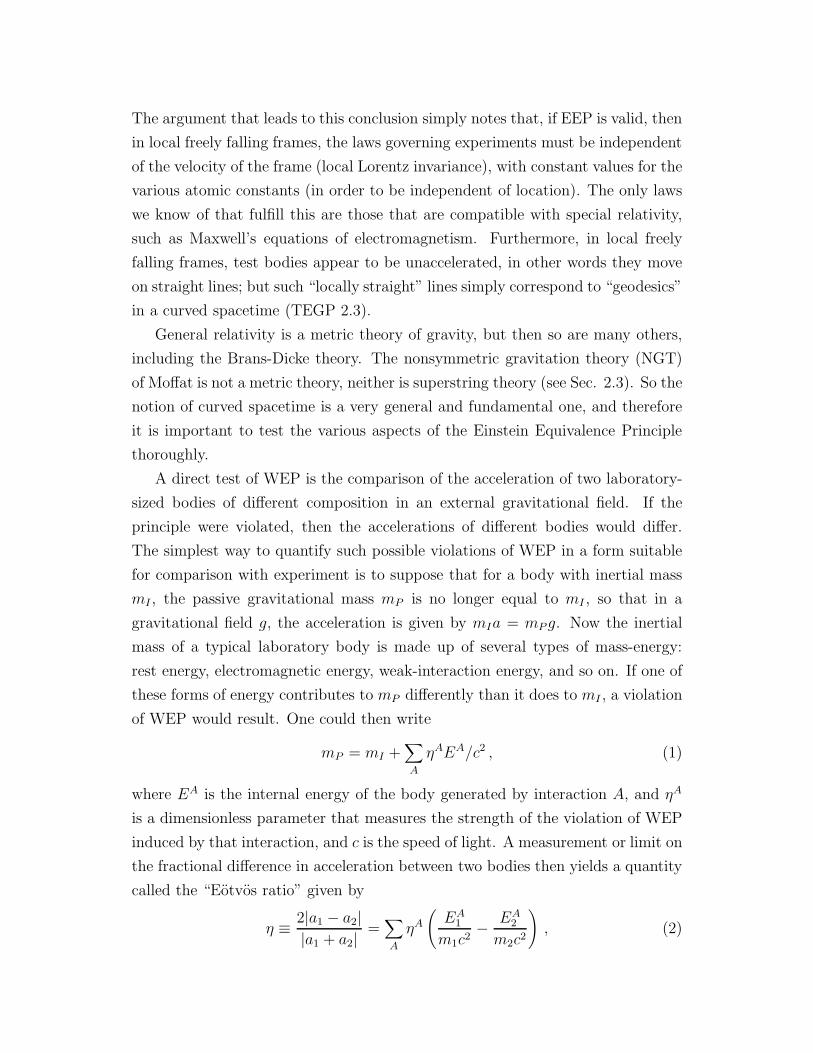
of WEP would result. One could then write
mP = mI +∑
A
ηAEA/c2 , (1)
where EA is the internal energy of the body generated by interaction A, and ηA
is a dimensionless parameter that measures the strength of the violation of WEP
induced by that interaction, and c is the speed of light. A measurement or limit on
the fractional difference in acceleration between two bodies then yields a quantity
called the “Eotvos ratio” given by
η ≡ 2|a1 − a2||a1 + a2|
=∑
A
ηA
(
EA1
m1c2− EA
2
m2c2
)
, (2)

where we drop the subscript I from the inertial masses. Thus, experimental limits
on η place limits on the WEP-violation parameters ηA.
Many high-precision Eotvos-type experiments have been performed, from the
pendulum experiments of Newton, Bessel and Potter, to the classic torsion-balance
measurements of Eotvos, Dicke, Braginsky and their collaborators. In the modern
torsion-balance experiments, two objects of different composition are connected
by a rod or placed on a tray and suspended in a horizontal orientation by a fine
wire. If the gravitational acceleration of the bodies differs, there will be a torque
induced on the suspension wire, related to the angle between the wire and the
direction of the gravitational acceleration g. If the entire apparatus is rotated
about some direction with angular velocity ω, the torque will be modulated with
period 2π/ω. In the experiments of Eotvos and his collaborators, the wire and g
were not quite parallel because of the centripetal acceleration on the apparatus
due to the Earth’s rotation; the apparatus was rotated about the direction of the
wire. In the Princeton (Dicke et al. ), and Moscow (Braginsky et al. ) experiments,
g was that of the Sun, and the rotation of the Earth provided the modulation of
the torque at a period of 24 hr (TEGP 2.4(a)). Beginning in the late 1980s,
numerous experiments were carried out primarily to search for a “fifth force” (see
Sec. 2.3), but their null results also constituted tests of WEP. In the “free-fall
Galileo experiment” performed at the University of Colorado, the relative free-fall
acceleration of two bodies made of uranium and copper was measured using a
laser interferometric technique. The “Eot-Wash” experiment carried out at the
University of Washington used a sophisticated torsion balance tray to compare the
accelerations of beryllium and copper toward local topography on Earth, movable
laboratory masses, the Sun and the galaxy.7 The resulting upper limits on η are
summarized in Figure 1 (TEGP 14.1; for a bibliography of experiments, see Ref.
8.
The second ingredient of EEP, local Lorentz invariance, can be said to be
tested every time that special relativity is confirmed in the laboratory. However,
many such experiments, especially in high-energy physics, are not “clean” tests,
because in many cases it is unlikely that a violation of Lorentz invariance could be
distinguished from effects due to the complicated strong and weak interactions.
However, there is one class of experiments that can be interpreted as “clean”,
high-precision tests of local Lorentz invariance. These are the “mass anisotropy”
experiments: the classic versions are the Hughes-Drever experiments, performed

19001920
19401960
19701980
19902000
10−8
10−9
10−10
10−11
10−12
10−13
10−14
YEAR OF EXPERIMENT
η
Eotvos
Renner
Princeton
Moscow
Boulder
Eot−Wash
Eot−Wash II
Free−fall
Fifth−force searches
LURE
TESTS OF THE WEAK EQUIVALENCE PR INCIPLE
η= a1−a2 (a1+a2)/2
Fig. 1. Selected tests of the Weak Equivalence Principle, showing bounds on
η, which measures fractional difference in acceleration of different materials or
bodies. Free-fall and Eot-Wash experiments originally performed to search for
fifth force. Hatched line shows current bounds on η for gravitating bodies from
lunar laser ranging (LURE).

in the period 1959-60 independently by Hughes and collaborators at Yale Univer-
sity, and by Drever at Glasgow University (TEGP 2.4(b)). Dramatically improved
versions were carried out during the late 1980s using laser-cooled trapped atom
techniques (TEGP 14.1). A simple and useful way of interpreting these experi-
ments is to suppose that the electromagnetic interactions suffer a slight violation
of Lorentz invariance, through a change in the speed of electromagnetic radiation
c relative to the limiting speed of material test particles (c0, chosen to be unity
via a choice of units), in other words, c 6= 1 (see Sec. 2.2.3). Such a violation
necessarily selects a preferred universal rest frame, presumably that of the cosmic
background radiation, through which we are moving at about 300 km/s. Such
a Lorentz-non-invariant electromagnetic interaction would cause shifts in the en-
ergy levels of atoms and nuclei that depend on the orientation of the quantization
axis of the state relative to our universal velocity vector, and on the quantum
numbers of the state. The presence or absence of such energy shifts can be ex-
amined by measuring the energy of one such state relative to another state that
is either unaffected or is affected differently by the supposed violation. One way
is to look for a shifting of the energy levels of states that are ordinarily equally
spaced, such as the four J=3/2 ground states of the 7Li nucleus in a magnetic
field (Drever experiment); another is to compare the levels of a complex nucleus
with the atomic hyperfine levels of a hydrogen maser clock. These experiments
have all yielded extremely accurate results, quoted as limits on the parameter
δ ≡ c−2 − 1 in Figure 2. Also included for comparison is the corresponding limit
obtained from Michelson-Morley type experiments.
Recent advances in atomic spectroscopy and atomic timekeeping have made it
possible to test LLI by checking the isotropy of the speed of light using one-way
propagation (as opposed to round-trip propagation, as in the Michelson-Morley
experiment). In one experiment, for example, the relative phases of two hydrogen
maser clocks at two stations of NASA ’s Deep Space Tracking Network were
compared over five rotations of the Earth by propagating a light signal one-way
along an ultrastable fiberoptic link connecting them (see Sec. 2.2.3). Although
the bounds from these experiments are not as tight as those from mass-anisotropy
experiments, they probe directly the fundamental postulates of special relativity,
and thereby of LLI. (TEGP 14.1).
The principle of local position invariance, the third part of EEP, can be tested
by the gravitational redshift experiment, the first experimental test of gravitation

19001920
19401960
19701980
19902000
10−2
10−6
10−10
10−14
10−18
10−22
10−26
YEAR OF EXPERIMENT
δ
Michelson−MorleyJoos
Hughes−Drever
Brillet−Hall
JPL
TESTS OF LOCAL LORENTZ INVAR IANCE
δ = c−2 − 1
TPACentrifuge
NIST
Harvard
U. Washington
Fig. 2. Selected tests of local Lorentz invariance showing bounds on parameter
δ, which measures degree of violation of Lorentz invariance in electromagnetism.
Michelson-Morley, Joos, and Brillet-Hall experiments test isotropy of round-trip
speed of light, the latter experiment using laser technology. Centrifuge, two-
photon absorption (TPA) and JPL experiments test isotropy of light speed using
one-way propagation. Remaining four experiments test isotropy of nuclear energy
levels. Limits assume speed of Earth of 300 km/s relative to the mean rest frame
of the universe.

proposed by Einstein. Despite the fact that Einstein regarded this as a crucial test
of GR, we now realize that it does not distinguish between GR and any other met-
ric theory of gravity, instead is a test only of EEP. A typical gravitational redshift
experiment measures the frequency or wavelength shift Z ≡ ∆ν/ν = −∆λ/λ be-
tween two identical frequency standards (clocks) placed at rest at different heights
in a static gravitational field. If the frequency of a given type of atomic clock is
the same when measured in a local, momentarily comoving freely falling frame
(Lorentz frame), independent of the location or velocity of that frame, then the
comparison of frequencies of two clocks at rest at different locations boils down to
a comparison of the velocities of two local Lorentz frames, one at rest with respect
to one clock at the moment of emission of its signal, the other at rest with respect
to the other clock at the moment of reception of the signal. The frequency shift
is then a consequence of the first-order Doppler shift between the frames. The
structure of the clock plays no role whatsoever. The result is a shift
Z = ∆U/c2 , (3)
where ∆U is the difference in the Newtonian gravitational potential between the
receiver and the emitter. If LPI is not valid, then it turns out that the shift can
be written
Z = (1 + α)∆U/c2 , (4)
where the parameter α may depend upon the nature of the clock whose shift is
being measured (see TEGP 2.4(c) for details).
The first successful, high-precision redshift measurement was the series of
Pound-Rebka-Snider experiments of 1960-1965, that measured the frequency shift
of gamma-ray photons from 57Fe as they ascended or descended the Jefferson
Physical Laboratory tower at Harvard University. The high accuracy achieved–
one percent–was obtained by making use of the Mossbauer effect to produce a
narrow resonance line whose shift could be accurately determined. Other exper-
iments since 1960 measured the shift of spectral lines in the Sun’s gravitational
field and the change in rate of atomic clocks transported aloft on aircraft, rockets
and satellites. Figure 3 summarizes the important redshift experiments that have
been performed since 1960 (TEGP 2.4(c)).
The most precise experiment to date was the Vessot-Levine rocket redshift
experiment that took place in June 1976. A hydrogen-maser clock was flown
on a rocket to an altitude of about 10,000 km and its frequency compared to

19601970
19801990
2000
10−1
10−2
10−3
10−4
10−5
YEAR OF EXPERIMENT
α
Pound−Rebka Millisecond Pulsar
TESTS OF LOCAL POSITION INVA RIANCE
H−maser
NullRedshiftPound−Snider
Saturn
NullRedshift
Solar spectra
Clocks in rockets & planes
∆ν/ν = (1+α)∆U/c²
Fig. 3. Selected tests of local position invariance via gravitational redshift experi-
ments, showing bounds on α, which measures degree of deviation of redshift from
the formula ∆ν/ν = ∆U/c2.

a similar clock on the ground. The experiment took advantage of the masers’
frequency stability by monitoring the frequency shift as a function of altitude.
A sophisticated data acquisition scheme accurately eliminated all effects of the
first-order Doppler shift due to the rocket’s motion, while tracking data were used
to determine the payload’s location and the velocity (to evaluate the potential
difference ∆U , and the special relativistic time dilation). Analysis of the data
yielded a limit |α| < 2 × 10⁻⁴.
A “null” redshift experiment performed in 1978 tested whether the relative
rates of two different clocks depended upon position. Two hydrogen maser clocks
and an ensemble of three superconducting-cavity stabilized oscillator (scso) clocks
were compared over a 10-day period. During this period, the solar potential
U/c2 changed sinusoidally with a 24-hour period by 3 × 10⁻¹³ because of the
Earth’s rotation, and changed linearly at 3 × 10⁻¹² per day because the Earth is
90 degrees from perihelion in April. However, analysis of the data revealed no
variations of either type within experimental errors, leading to a limit on the LPI
violation parameter |αH −αSCSO| < 2×10⁻². This bound is likely to be improved
using more stable frequency standards.9,10 The varying gravitational redshift of
Earth-bound clocks relative to the highly stable Millisecond Pulsar, caused by
the Earth’s motion in the solar gravitational field around the Earth-Moon center
of mass (amplitude 4000 km), has been measured to about 10 percent, and the
redshift of stable oscillator clocks on the Voyager spacecraft caused by Saturn’s
gravitational field yielded a one percent test. The solar gravitational redshift has
been tested to about two percent using infrared oxygen triplet lines at the limb
of the Sun, and to one percent using oscillator clocks on the Galileo spacecraft
(TEGP 2.4(c) and 14.1(a)).
Modern advances in navigation using Earth-orbiting atomic clocks and ac-
curate time-transfer must routinely take gravitational redshift and time-dilation
effects into account. For example, the Global Positioning System (GPS) provides
absolute accuracies of around 15 m (even better in its military mode) anywhere
on Earth, which corresponds to 50 nanoseconds in time accuracy at all times. Yet
the difference in rate between satellite and ground clocks as a result of special and
general relativistic effects is a whopping 40 microseconds per day (60µs from the
gravitational redshift, and −20µs from time dilation). If these effects were not
accurately accounted for, GPS would fail to function at its stated accuracy. This
represents a welcome practical application of GR!

Limit on k/k
per Hubble time
Constant k 1.2 × 10¹⁰yr Method
Fine structure constant 4 × 10⁻⁴ H-maser vs Hg ion clock10
α = e2/hc 6 × 10⁻⁷ Oklo Natural Reactor11
6 × 10⁻⁵ 21-cm vs molecular absorption
at Z = 0.7 (Ref. 12)
Weak interaction constant 1 187Re, 40K decay rates
β = Gfm2pc/h
3 0.1 Oklo Natural Reactor11
0.06 Big bang nucleosynthesis13
e-p mass ratio 1 Mass shift in quasar
spectra at Z ∼ 2
Proton g-factor (gp) 10−5 21-cm vs molecular absorption
at Z = 0.7 (Ref. 12)
Table 1. Bounds on cosmological variation of fundamental constants of non-
gravitational physics. For references to earlier work, see TEGP 2.4(c).
Local position invariance also refers to position in time. If LPI is satisfied, the
fundamental constants of non-gravitational physics should be constants in time.
Table 1 shows current bounds on cosmological variations in selected dimensionless
constants. For discussion and references to early work, see TEGP 2.4(c).
2.2 Theoretical Frameworks for Analyzing EEP
2.2.1 Schiff’s Conjecture
Because the three parts of the Einstein equivalence principle discussed above are
so very different in their empirical consequences, it is tempting to regard them
as independent theoretical principles. On the other hand, any complete and self-
consistent gravitation theory must possess sufficient mathematical machinery to
make predictions for the outcomes of experiments that test each principle, and
because there are limits to the number of ways that gravitation can be meshed
with the special relativistic laws of physics, one might not be surprised if there
were theoretical connections between the three sub-principles. For instance, the
same mathematical formalism that produces equations describing the free fall of
a hydrogen atom must also produce equations that determine the energy levels
of hydrogen in a gravitational field, and thereby the ticking rate of a hydrogen
maser clock. Hence a violation of EEP in the fundamental machinery of a theory
that manifests itself as a violation of WEP might also be expected to show up as
a violation of local position invariance. Around 1960, Schiff conjectured that this
kind of connection was a necessary feature of any self-consistent theory of grav-
ity. More precisely, Schiff’s conjecture states that any complete, self-consistent
theory of gravity that embodies WEP necessarily embodies EEP. In other words,
the validity of WEP alone guarantees the validity of local Lorentz and position
invariance, and thereby of EEP.
If Schiff’s conjecture is correct, then Eotvos experiments may be seen as the
direct empirical foundation for EEP, hence for the interpretation of gravity as a
curved-spacetime phenomenon. Of course, a rigorous proof of such a conjecture
is impossible (indeed, some special counter-examples are known) yet a number of
powerful “plausibility” arguments can be formulated.
The most general and elegant of these arguments is based upon the assumption
of energy conservation. This assumption allows one to perform very simple cyclic
gedanken experiments in which the energy at the end of the cycle must equal that
at the beginning of the cycle. This approach was pioneered by Dicke, Nordtvedt
and Haugan. A system in a quantum state A decays to state B, emitting a quan-
tum of frequency ν. The quantum falls a height H in an external gravitational
field and is shifted to frequency ν ′, while the system in state B falls with accel-
eration gB. At the bottom, state A is rebuilt out of state B, the quantum of
frequency ν ′, and the kinetic energy mBgBH that state B has gained during its
fall. The energy left over must be exactly enough, mAgAH , to raise state A to
its original location. (Here an assumption of local Lorentz invariance permits the
inertial masses mA and mB to be identified with the total energies of the bodies.)
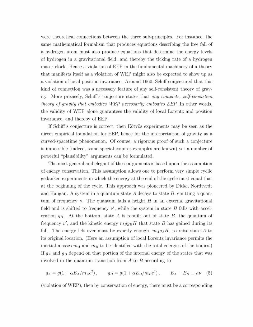
If gA and gB depend on that portion of the internal energy of the states that was
involved in the quantum transition from A to B according to
gA = g(1 + αEA/mAc2) , gB = g(1 + αEB/mBc
2) , EA −EB ≡ hν (5)
(violation of WEP), then by conservation of energy, there must be a corresponding

violation of LPI in the frequency shift of the form (to lowest order in hν/mc2)
Z = (ν ′ − ν)/ν′ = (1 + α)gH/c2 = (1 + α)∆U/c2 . (6)
Haugan generalized this approach to include violations of LLI (TEGP 2.5).
2.2.2 The THǫµ Formalism
The first successful attempt to prove Schiff’s conjecture more formally was made
by Lightman and Lee. They developed a framework called the THǫµ formalism
that encompasses all metric theories of gravity and many non-metric theories (Box
1). It restricts attention to the behavior of charged particles (electromagnetic
interactions only) in an external static spherically symmetric (SSS) gravitational
field, described by a potential U . It characterizes the motion of the charged
particles in the external potential by two arbitrary functions T (U) and H(U),
and characterizes the response of electromagnetic fields to the external potential
(gravitationally modified Maxwell equations) by two functions ǫ(U) and µ(U).
The forms of T , H , ǫ and µ vary from theory to theory, but every metric theory
satisfies
ǫ = µ = (H/T )1/2 , (7)
for all U . This consequence follows from the action of electrodynamics with a
“minimal” or metric coupling:
I = −∑
a
m0a
∫
(gµνvµav
νa)1/2dt+
∑
a
ea
∫
Aµ(xνa)v
µadt
− 1
16π
∫ √−ggµαgνβFµνFαβd4x , (8)
where the variables are defined in Box 1, and where Fµν ≡ Aν,µ − Aµ,ν . By
identifying g00 = T and gij = Hδij in a SSS field, Fi0 = Ei and Fij = ǫijkBk, one
obtains Equation 7.
Conversely, every theory within this class that satisfies Equation 7 can have
its electrodynamic equations cast into “metric” form. Lightman and Lee then
calculated explicitly the rate of fall of a “test” body made up of interacting charged
particles, and found that the rate was independent of the internal electromagnetic
structure of the body (WEP) if and only if Equation 7 was satisfied. In other words
WEP → EEP and Schiff’s conjecture was verified, at least within the restrictions
built into the formalism.

Box 1. The THǫµ Formalism
1. Coordinate System and Conventions:
x0 = t = time coordinate associated with the static nature of the static spheri-
cally symmetric (sss) gravitational field; x = (x, y, z) = isotropic quasi-Cartesian
spatial coordinates; spatial vector and gradient operations as in Cartesian space.
2. Matter and Field Variables:
• m0a = rest mass of particle a.
• ea = charge of particle a.
• xµa(t) = world line of particle a.
• vµa = dxµ
a/dt = coordinate velocity of particle a.
• Aµ = electromagnetic vector potential; E = ∇A0 − ∂A/∂t , B = ∇× A
3. Gravitational Potential: U(x)
4. Arbitrary Functions:
T (U), H(U), ǫ(U), µ(U); EEP is satisfied iff ǫ = µ = (H/T )1/2 for all U .
5. Action:
I = −∑
a
m0a
∫
(T−Hv2a)
1/2dt+∑
a
ea
∫
Aµ(xνa)v
µa dt+(8π)−1
∫
(ǫE2−µ−1B2)d4x .
6. Non-Metric Parameters:
Γ0 = −c20(∂/∂U) ln[ǫ(T/H)1/2]0 ,
Λ0 = −c20(∂/∂U) ln[µ(T/H)1/2]0 ,
Υ0 = 1 − (TH−1ǫµ)0 ,
where c0 = (T0/H0)1/2 and subscript “0” refers to a chosen point in space. If EEP
is satisfied, Γ0 ≡ Λ0 ≡ Υ0 ≡ 0.

Certain combinations of the functions T , H , ǫ and µ reflect different aspects
of EEP. For instance, position or U -dependence of either of the combinations
ǫ(T/H)1/2 and µ(T/H)1/2 signals violations of LPI, the first combination playing
the role of the locally measured electric charge or fine structure constant. The
“non-metric parameters” Γ0 and Λ0 (Box 1) are measures of such violations of
EEP. Similarly, if the parameter Υ0 ≡ 1− (TH−1ǫµ)0 is non-zero anywhere, then
violations of LLI will occur. This parameter is related to the difference between
the speed of light, c, and the limiting speed of material test particles, co, given by
c = (ǫ0µ0)−1/2 , co = (T0/H0)
1/2 . (9)
In many applications, by suitable definition of units, c0 can be set equal to unity.
If EEP is valid, Γ0 ≡ Λ0 ≡ Υ0 = 0 everywhere.
The rate of fall of a composite spherical test body of electromagnetically in-
teracting particles then has the form
a = (mP/m)∇U , (10)
mP/m = 1 + (EESB /Mc20)[2Γ0 −
8
3Υ0] + (EMS
B /Mc20)[2Λ0 −4
3Υ0] + . . . ,(11)
where EESB and EMS
B are the electrostatic and magnetostatic binding energies of
the body, given by
EESB = −1
4T
1/20 H−1
0 ǫ−10
⟨
∑
ab
eaebr−1ab
⟩
, (12)
EMSB = −1
8T
1/20 H−1
0 µ0
⟨
∑
ab
eaebr−1ab [va · vb + (va · nab)(vb · nab)]
⟩
, (13)
where rab = |xa−xb|, nab = (xa−xb)/rab, and the angle brackets denote an expec-
tation value of the enclosed operator for the system’s internal state. Eotvos exper-
iments place limits on the WEP-violating terms in Equation 11, and ultimately
place limits on the non-metric parameters |Γ0| < 2 × 10⁻¹⁰ and |Λ0| < 3 × 10⁻⁶.
(We set Υ0 = 0 because of very tight constraints on it from tests of LLI .) These
limits are sufficiently tight to rule out a number of non-metric theories of gravity
thought previously to be viable (TEGP 2.6(f)).
The THǫµ formalism also yields a gravitationally modified Dirac equation that
can be used to determine the gravitational redshift experienced by a variety of
atomic clocks. For the redshift parameter α (Equation 4), the results are (TEGP
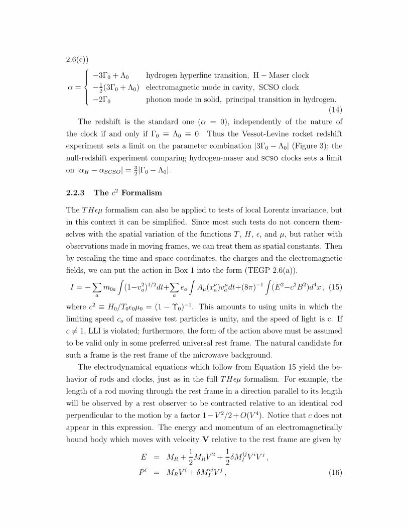
2.6(c))
α =
−3Γ0 + Λ0 hydrogen hyperfine transition, H − Maser clock
−12(3Γ0 + Λ0) electromagnetic mode in cavity, SCSO clock
−2Γ0 phonon mode in solid, principal transition in hydrogen.
(14)
The redshift is the standard one (α = 0), independently of the nature of
the clock if and only if Γ0 ≡ Λ0 ≡ 0. Thus the Vessot-Levine rocket redshift
experiment sets a limit on the parameter combination |3Γ0 − Λ0| (Figure 3); the
null-redshift experiment comparing hydrogen-maser and scso clocks sets a limit
on |αH − αSCSO| = 32|Γ0 − Λ0|.
2.2.3 The c2 Formalism
The THǫµ formalism can also be applied to tests of local Lorentz invariance, but
in this context it can be simplified. Since most such tests do not concern them-
selves with the spatial variation of the functions T , H , ǫ, and µ, but rather with
observations made in moving frames, we can treat them as spatial constants. Then
by rescaling the time and space coordinates, the charges and the electromagnetic
fields, we can put the action in Box 1 into the form (TEGP 2.6(a)).
I = −∑
a
m0a
∫
(1−v2a)
1/2dt+∑
a
ea
∫
Aµ(xνa)v
µadt+(8π)−1
∫
(E2−c2B2)d4x , (15)
where c2 ≡ H0/T0ǫ0µ0 = (1 − Υ0)−1. This amounts to using units in which the
limiting speed co of massive test particles is unity, and the speed of light is c. If
c 6= 1, LLI is violated; furthermore, the form of the action above must be assumed
to be valid only in some preferred universal rest frame. The natural candidate for
such a frame is the rest frame of the microwave background.
The electrodynamical equations which follow from Equation 15 yield the be-
havior of rods and clocks, just as in the full THǫµ formalism. For example, the
length of a rod moving through the rest frame in a direction parallel to its length
will be observed by a rest observer to be contracted relative to an identical rod
perpendicular to the motion by a factor 1−V 2/2+O(V 4). Notice that c does not
appear in this expression. The energy and momentum of an electromagnetically
bound body which moves with velocity V relative to the rest frame are given by
E = MR +1
2MRV
2 +1
2δM ij
I ViV j ,
P i = MRVi + δM ij
I Vj , (16)

where MR = M0 − EESB , M0 is the sum of the particle rest masses, EES
B is the
electrostatic binding energy of the system (Equation 12 with T1/20 H0ǫ
−10 = 1), and
δM ijI = −2(
1
c2− 1)[
4
3EES
B δij + EESijB ] , (17)
where
EESijB = −1
4
⟨
∑
ab
eaebr−1ab
(
(niabn
jab −
1
3δij)
⟩
. (18)
Note that (c−2 − 1) corresponds to the parameter δ plotted in Figure 2.
The electrodynamics given by Equation 15 can also be quantized, so that we
may treat the interaction of photons with atoms via perturbation theory. The
energy of a photon is h times its frequency ω, while its momentum is hω/c. Using
this approach, one finds that the difference in round trip travel times of light along
the two arms of the interferometer in the Michelson-Morley experiment is given
by L0(v2/c)(c−2 − 1). The experimental null result then leads to the bound on
(c−2 − 1) shown on Figure 2. Similarly the anisotropy in energy levels is clearly
illustrated by the tensorial terms in Equations 16 and 18; by evaluating EESijB
for each nucleus in the various Hughes-Drever-type experiments and comparing
with the experimental limits on energy differences, one obtains the extremely tight
bounds also shown on Figure 2.
The behavior of moving atomic clocks can also be analysed in detail, and
bounds on (c−2 − 1) can be placed using results from tests of time dilation and
of the propagation of light. In some cases, it is advantageous to combine the c2
framework with a “kinematical” viewpoint that treats a general class of boost
transformations between moving frames. Such kinematical approaches have been
discussed by Robertson, Mansouri and Sexl, and Will (see Ref. 14).
For example, in the “JPL” experiment, in which the phases of two hydrogen
masers connected by a fiberoptic link were compared as a function of the Earth’s
orientation, the predicted phase difference as a function of direction is, to first
order in V, the velocity of the Earth through the cosmic background,
∆φ/φ ≈ −4
3(1 − c2)(V · n − V · n0) , (19)
where φ = 2πνL, ν is the maser frequency, L = 21 km is the baseline, and where
n and n0 are unit vectors along the direction of propagation of the light, at a given
time, and at the initial time of the experiment, respectively. The observed limit on
a diurnal variation in the relative phase resulted in the bound |c−2−1| < 3×10⁻⁴.

Tighter bounds were obtained from a “two-photon absorption” (TPA) experiment,
and a 1960s series of “Mossbauer-rotor” experiments, which tested the isotropy of
time dilation between a gamma ray emitter on the rim of a rotating disk and an
absorber placed at the center.14
2.3 EEP, Particle Physics, and the Search for New Inter-
actions
In 1986, as a result of a detailed reanalysis of Eotvos’ original data, Fischbach
et al. suggested the existence of a fifth force of nature, with a strength of about a
percent that of gravity, but with a range (as defined by the range λ of a Yukawa
potential, e−r/λ/r) of a few hundred meters. This proposal dovetailed with earlier
hints of a deviation from the inverse-square law of Newtonian gravitation derived
from measurements of the gravity profile down deep mines in Australia, and with
ideas from particle physics suggesting the possible presence of very low-mass par-
ticles with gravitational-strength couplings. During the next four years numerous
experiments looked for evidence of the fifth force by searching for composition-
dependent differences in acceleration, with variants of the Eotvos experiment or
with free-fall Galileo-type experiments. Although two early experiments reported
positive evidence, the others all yielded null results. Over the range between one
and 104 meters, the null experiments produced upper limits on the strength of
a postulated fifth force between 10−3 and 10−6 of the strength of gravity. Inter-
preted as tests of WEP (corresponding to the limit of infinite-range forces), the
results of the free-fall Galileo experiment, and of the Eot-Wash III experiment are
shown in Figure 1. At the same time, tests of the inverse-square law of gravity
were carried out by comparing variations in gravity measurements up tall towers
or down mines or boreholes with gravity variations predicted using the inverse
square law together with Earth models and surface gravity data mathematically
“continued” up the tower or down the hole. Despite early reports of anomalies,
independent tower, borehole and seawater measurements now show no evidence
of a deviation. The consensus at present is that there is no credible experimen-
tal evidence for a fifth force of nature. For reviews and bibliographies, see Refs.
8,15,16 and 17.
Nevertheless, theoretical evidence continues to mount that EEP is likely to be
violated at some level, whether by quantum gravity effects, by effects arising from

string theory, or by hitherto undetected interactions, albeit at levels below those
that motivated the fifth-force searches. Roughly speaking, in addition to the pure
Einsteinian gravitational interaction, which respects EEP, theories such as string
theory predict other interactions which do not. In string theory, for example, the
existence of such EEP-violating fields is assured, but the theory is not yet mature
enough to enable calculation of their strength (relative to gravity), or their range
(whether they are long range, like gravity, or short range, like the nuclear and
weak interactions, or too short-range to be detectable) (for further discussion see
Ref. 6).
In one simple example, one can write the Lagrangian for the low-energy limit
of string theory in the so-called “Einstein frame”, in which the gravitational La-
grangian is purely general relativistic:
L =√−g
(
gµν
[
12κRµν − 1
2G(ϕ)∂µϕ∂νϕ
]
− U(ϕ)gµν gαβFµαFνβ
+¯ψ[
ieµaγ
a(∂µ + Ωµ + qAµ) − M(ϕ)]
ψ)
, (20)
where gµν is the non-physical metric, Rµν is the Ricci tensor derived from it, ϕ
is a dilaton field, and G, U and M are functions of ϕ. The Lagrangian includes
that for the electromagnetic field Fµν , and that for particles, written in terms of
Dirac spinors ψ. This is not a metric representation because of the coupling of
ϕ to matter via M(ϕ) and U(ϕ). A conformal transformation gµν = F (ϕ)gµν ,
ψ = F (ϕ)−3/4ψ, puts the Lagrangian in the form (“Jordan” frame)
L =√−g
(
gµν
[
12κF (ϕ)Rµν − 1
2F (ϕ)G(ϕ)∂µϕ∂νϕ+ 3
4κF (ϕ)∂µF∂νF
]
−U(ϕ)gµνgαβFµαFνβ + ψ[
ieµaγ
a(∂µ + Ωµ + qAµ) − M(ϕ)F 1/2
]
ψ)
. (21)
One may choose F (ϕ) = const/M(ϕ)2 so that the particle Lagrangian takes the
metric form (no coupling to ϕ), but the electromagnetic Lagrangian will still
couple non-metrically to U(ϕ). The gravitational Lagrangian here takes the form
of a scalar-tensor theory (Sec. 3.3.2). But the non-metric electromagnetic term
will, in general, produce violations of EEP.
Thus, EEP and related tests are now viewed as ways to discover or place con-
straints on new physical interactions, or as a branch of “non-accelerator particle
physics”, searching for the possible imprints of high-energy particle effects in the
low-energy realm of gravity. Whether current or proposed experiments can ac-
tually probe these phenomena meaningfully is an open question at the moment,

largely because of a dearth of firm theoretical predictions. Despite this uncer-
tainty, a number of experimental possibilities are being explored.
The concept of an equivalence principle experiment in space has been devel-
oped, with the potential to test WEP to 10−18. Known generically as Satellite
Test of the Equivalence Principle (STEP), various versions of the project are
under consideration as possible joint efforts of NASA and the European Space
Agency (ESA). The gravitational redshift could be improved to the 10−10 level
using atomic clocks on board a spacecraft which would travel to within four so-
lar radii of the Sun. Laboratory tests of the gravitational inverse square law at
sub-millimeter scales are being developed as ways to search for new short-range
interactions; the challenge of these experiments is to distinguish gravitation-like
interactions from electromagnetic and quantum mechanical (Casimir) effects.
3 Tests of Post-Newtonian Gravity
3.1 Metric Theories of Gravity and the Strong Equiva-
lence Principle
3.1.1 Universal Coupling and the Metric Postulates
The overwhelming empirical evidence supporting the Einstein equivalence prin-
ciple, discussed in the previous section, supports the conclusion that the only
theories of gravity that have a hope of being viable are metric theories, or possi-
bly theories that are metric apart from possible weak or short-range non-metric
couplings (as in string theory). Therefore for the remainder of these lectures, we
shall turn our attention exclusively to metric theories of gravity, which assume
that (i) there exists a symmetric metric, (ii) test bodies follow geodesics of the
metric, and (iii) in local Lorentz frames, the non-gravitational laws of physics are
those of special relativity.
The property that all non-gravitational fields should couple in the same manner
to a single gravitational field is sometimes called “universal coupling”. Because of
it, one can discuss the metric as a property of spacetime itself rather than as a field
over spacetime. This is because its properties may be measured and studied using
a variety of different experimental devices, composed of different non-gravitational
fields and particles, and, because of universal coupling, the results will be inde-

pendent of the device. Thus, for instance, the proper time between two events is
a characteristic of spacetime and of the location of the events, not of the clocks
used to measure it.
Consequently, if EEP is valid, the non-gravitational laws of physics may be
formulated by taking their special relativistic forms in terms of the Minkowski
metric η and simply “going over” to new forms in terms of the curved spacetime
metric g, using the mathematics of differential geometry. The details of this “going
over” can be found in standard textbooks (Refs. 18,19; TEGP 3.2)
3.1.2 The Strong Equivalence Principle
In any metric theory of gravity, matter and non-gravitational fields respond only to
the spacetime metric g. In principle, however, there could exist other gravitational
fields besides the metric, such as scalar fields, vector fields, and so on. If, by our
strict definition of metric theory, matter does not couple to these fields what can
their role in gravitation theory be? Their role must be that of mediating the
manner in which matter and non-gravitational fields generate gravitational fields
and produce the metric; once determined, however, the metric alone acts back on
the matter in the manner prescribed by EEP.
What distinguishes one metric theory from another, therefore, is the number
and kind of gravitational fields it contains in addition to the metric, and the
equations that determine the structure and evolution of these fields. From this
viewpoint, one can divide all metric theories of gravity into two fundamental
classes: “purely dynamical” and “prior-geometric”.
By “purely dynamical metric theory” we mean any metric theory whose grav-
itational fields have their structure and evolution determined by coupled partial
differential field equations. In other words, the behavior of each field is influ-
enced to some extent by a coupling to at least one of the other fields in the
theory. By “prior geometric” theory, we mean any metric theory that contains
“absolute elements”, fields or equations whose structure and evolution are given
a priori, and are independent of the structure and evolution of the other fields of
the theory. These “absolute elements” typically include flat background metrics
η, cosmic time coordinates t, algebraic relationships among otherwise dynamical
fields, such as gµν = hµν + kµkν, where hµν and kµ may be dynamical fields.
General relativity is a purely dynamical theory since it contains only one grav-

itational field, the metric itself, and its structure and evolution are governed by
partial differential equations (Einstein’s equations). Brans-Dicke theory and its
generalizations are purely dynamical theories; the field equation for the metric
involves the scalar field (as well as the matter as source), and that for the scalar
field involves the metric. Rosen’s bimetric theory is a prior-geometric theory: it
has a non-dynamical, Riemann-flat background metric, η, and the field equations
for the physical metric g involve η.
By discussing metric theories of gravity from this broad point of view, it is
possible to draw some general conclusions about the nature of gravity in differ-
ent metric theories, conclusions that are reminiscent of the Einstein equivalence
principle, but that are subsumed under the name “strong equivalence principle”.
Consider a local, freely falling frame in any metric theory of gravity. Let this
frame be small enough that inhomogeneities in the external gravitational fields
can be neglected throughout its volume. On the other hand, let the frame be large
enough to encompass a system of gravitating matter and its associated gravita-
tional fields. The system could be a star, a black hole, the solar system or a
Cavendish experiment. Call this frame a “quasi-local Lorentz frame” . To deter-
mine the behavior of the system we must calculate the metric. The computation
proceeds in two stages. First we determine the external behavior of the metric and
gravitational fields, thereby establishing boundary values for the fields generated
by the local system, at a boundary of the quasi-local frame “far” from the local
system. Second, we solve for the fields generated by the local system. But because
the metric is coupled directly or indirectly to the other fields of the theory, its
structure and evolution will be influenced by those fields, and in particular by the
boundary values taken on by those fields far from the local system. This will be
true even if we work in a coordinate system in which the asymptotic form of gµν
in the boundary region between the local system and the external world is that
of the Minkowski metric. Thus the gravitational environment in which the local
gravitating system resides can influence the metric generated by the local system
via the boundary values of the auxiliary fields. Consequently, the results of local
gravitational experiments may depend on the location and velocity of the frame
relative to the external environment. Of course, local non-gravitational experi-
ments are unaffected since the gravitational fields they generate are assumed to
be negligible, and since those experiments couple only to the metric, whose form
can always be made locally Minkowskian at a given spacetime event. Local grav-

itational experiments might include Cavendish experiments, measurement of the
acceleration of massive self-gravitating bodies, studies of the structure of stars and
planets, or analyses of the periods of “gravitational clocks”. We can now make
several statements about different kinds of metric theories.
(i) A theory which contains only the metric g yields local gravitational physics
which is independent of the location and velocity of the local system. This follows
from the fact that the only field coupling the local system to the environment
is g, and it is always possible to find a coordinate system in which g takes the
Minkowski form at the boundary between the local system and the external envi-
ronment. Thus the asymptotic values of gµν are constants independent of location,
and are asymptotically Lorentz invariant, thus independent of velocity. General
relativity is an example of such a theory.
(ii) A theory which contains the metric g and dynamical scalar fields ϕA yields
local gravitational physics which may depend on the location of the frame but
which is independent of the velocity of the frame. This follows from the asymptotic
Lorentz invariance of the Minkowski metric and of the scalar fields, but now the
asymptotic values of the scalar fields may depend on the location of the frame.
An example is Brans-Dicke theory, where the asymptotic scalar field determines
the effective value of the gravitational constant, which can thus vary as ϕ varies.
(iii) A theory which contains the metric g and additional dynamical vector or
tensor fields or prior-geometric fields yields local gravitational physics which may
have both location and velocity-dependent effects.
These ideas can be summarized in the strong equivalence principle (SEP),
which states that (i) WEP is valid for self-gravitating bodies as well as for test
bodies, (ii) the outcome of any local test experiment is independent of the velocity
of the (freely falling) apparatus, and (iii) the outcome of any local test experiment
is independent of where and when in the universe it is performed. The distinction
between SEP and EEP is the inclusion of bodies with self-gravitational interac-
tions (planets, stars) and of experiments involving gravitational forces (Cavendish
experiments, gravimeter measurements). Note that SEP contains EEP as the spe-
cial case in which local gravitational forces are ignored.
The above discussion of the coupling of auxiliary fields to local gravitating
systems indicates that if SEP is strictly valid, there must be one and only one
gravitational field in the universe, the metric g. These arguments are only sug-
gestive however, and no rigorous proof of this statement is available at present.

Empirically it has been found that every metric theory other than GR introduces
auxiliary gravitational fields, either dynamical or prior geometric, and thus pre-
dicts violations of SEP at some level (here we ignore quantum-theory inspired
modifications to GR involving “R2” terms). General relativity seems to be the
only metric theory that embodies SEP completely. This lends some credence to
the conjecture SEP → General Relativity. In Sec. 3.6, we shall discuss experi-
mental evidence for the validity of SEP.
3.2 The Parametrized Post-Newtonian Formalism
Despite the possible existence of long-range gravitational fields in addition to
the metric in various metric theories of gravity, the postulates of those theories
demand that matter and non-gravitational fields be completely oblivious to them.
The only gravitational field that enters the equations of motion is the metric g.
The role of the other fields that a theory may contain can only be that of helping to
generate the spacetime curvature associated with the metric. Matter may create
these fields, and they plus the matter may generate the metric, but they cannot
act back directly on the matter. Matter responds only to the metric.
Thus the metric and the equations of motion for matter become the primary
entities for calculating observable effects, and all that distinguishes one metric
theory from another is the particular way in which matter and possibly other
gravitational fields generate the metric.
The comparison of metric theories of gravity with each other and with ex-
periment becomes particularly simple when one takes the slow-motion, weak-field
limit. This approximation, known as the post-Newtonian limit, is sufficiently
accurate to encompass most solar-system tests that can be performed in the fore-
seeable future. It turns out that, in this limit, the spacetime metric g predicted
by nearly every metric theory of gravity has the same structure. It can be written
as an expansion about the Minkowski metric (ηµν = diag(−1, 1, 1, 1)) in terms
of dimensionless gravitational potentials of varying degrees of smallness. These
potentials are constructed from the matter variables (Box 2) in imitation of the
Newtonian gravitational potential
U(x, t) ≡∫
ρ(x′, t)|x− x′|−1d3x′ . (22)
The “order of smallness” is determined according to the rules U ∼ v2 ∼ Π ∼p/ρ ∼ O(2), vi ∼ |d/dt|/|d/dx| ∼ 0(1), and so on.

Value Value
in semi- in fully-
What it measures Value conservative conservative
Parameter relative to GR in GR theories theories
γ How much space-curvature 1 γ γ
produced by unit rest mass?
β How much “nonlinearity” 1 β β
in the superposition
law for gravity?
ξ Preferred-location effects? 0 ξ ξ
α1 Preferred-frame effects? 0 α1 0
α2 0 α2 0
α3 0 0 0
α3 Violation of conservation 0 0 0
ζ1 of total momentum? 0 0 0
ζ2 0 0 0
ζ3 0 0 0
ζ4 0 0 0
Table 2. The PPN Parameters and their significance (note that α3 has been shown
twice to indicate that it is a measure of two effects)

A consistent post-Newtonian limit requires determination of g00 correct through
O(4), g0i through O(3) and gij through O(2) (for details see TEGP 4.1). The only
way that one metric theory differs from another is in the numerical values of
the coefficients that appear in front of the metric potentials. The parametrized
post-Newtonian (PPN ) formalism inserts parameters in place of these coefficients,
parameters whose values depend on the theory under study. In the current version
of the PPN formalism, summarized in Box 2, ten parameters are used, chosen in
such a manner that they measure or indicate general properties of metric theories
of gravity (Table 2). The parameters γ and β are the usual Eddington-Robertson-
Schiff parameters used to describe the “classical” tests of GR; ξ is non-zero in any
theory of gravity that predicts preferred-location effects such as a galaxy-induced
anisotropy in the local gravitational constant GL (also called “Whitehead” ef-
fects); α1, α2, α3 measure whether or not the theory predicts post-Newtonian
preferred-frame effects; α3, ζ1, ζ2, ζ3, ζ4 measure whether or not the theory pre-
dicts violations of global conservation laws for total momentum. In Table 2 we
show the values these parameters take (i) in GR, (ii) in any theory of gravity
that possesses conservation laws for total momentum, called “semi-conservative”
(any theory that is based on an invariant action principle is semi-conservative,
and (iii) in any theory that in addition possesses six global conservation laws for
angular momentum, called “fully conservative” (such theories automatically pre-
dict no post-Newtonian preferred-frame effects). Semi-conservative theories have
five free PPN parameters (γ, β, ξ, α1, α2) while fully conservative theories have
three (γ, β , ξ).
The PPN formalism was pioneered by Kenneth Nordtvedt, who studied the
post-Newtonian metric of a system of gravitating point masses, extending earlier
work by Eddington, Robertson and Schiff (TEGP 4.2). A general and unified ver-
sion of the PPN formalism was developed by Will and Nordtvedt. The canonical
version, with conventions altered to be more in accord with standard textbooks
such as mtw, is discussed in detail in TEGP, Chapter 4. Other versions of the PPN
formalism have been developed to deal with point masses with charge, fluid with
anisotropic stresses, bodies with strong internal gravity, and post-post-Newtonian
effects (TEGP 4.2, 14.2).

Box 2. The Parametrized Post-Newtonian Formalism
1. Coordinate System: The framework uses a nearly globally Lorentz coordinate
system in which the coordinates are (t, x1, x2, x3). Three-dimensional, Euclidean
vector notation is used throughout. All coordinate arbitrariness (“gauge freedom”)
has been removed by specialization of the coordinates to the standard PPN gauge
(TEGP 4.2). Units are chosen so that G = c = 1, where G is the physically
measured Newtonian constant far from the solar system.
2. Matter Variables:
• ρ = density of rest mass as measured in a local freely falling frame momentarily
comoving with the gravitating matter.
• vi = (dxi/dt) = coordinate velocity of the matter.
• wi = coordinate velocity of PPN coordinate system relative to the mean rest-
frame of the universe.
• p = pressure as measured in a local freely falling frame momentarily comoving
with the matter.
• Π = internal energy per unit rest mass. It includes all forms of non-rest-mass,
non-gravitational energy, e.g. energy of compression and thermal energy.
3. PPN Parameters:
γ , β , ξ , α1 , α2 , α3 , ζ1 , ζ2 , ζ3 , ζ4 .
4. Metric:
g00 = −1 + 2U − 2βU2 − 2ξΦW + (2γ + 2 + α3 + ζ1 − 2ξ)Φ1
+2(3γ − 2β + 1 + ζ2 + ξ)Φ2 + 2(1 + ζ3)Φ3 + 2(3γ + 3ζ4 − 2ξ)Φ4
−(ζ1 − 2ξ)A− (α1 − α2 − α3)w2U − α2w
iwjUij + (2α3 − α1)wiVi
g0i = −1
2(4γ + 3 + α1 − α2 + ζ1 − 2ξ)Vi −
1
2(1 + α2 − ζ1 + 2ξ)Wi
−1
2(α1 − 2α2)w
iU − α2wjUij
gij = (1 + 2γU)δij
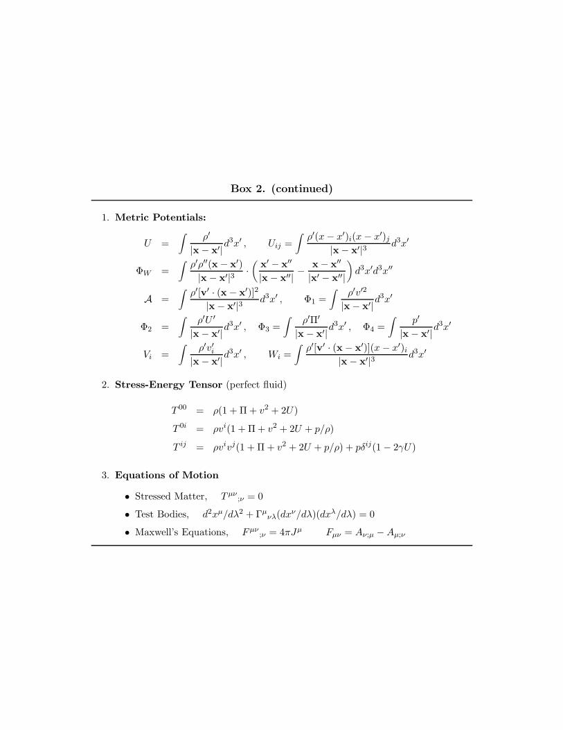
Box 2. (continued)
1. Metric Potentials:
U =
∫
ρ′
|x − x′|d3x′ , Uij =
∫
ρ′(x − x′)i(x − x′)j|x− x′|3 d3x′
ΦW =
∫
ρ′ρ′′(x − x′)
|x − x′|3 ·(
x′ − x′′
|x − x′′| −x − x′′
|x′ − x′′|
)
d3x′d3x′′
A =
∫
ρ′[v′ · (x − x′)]2
|x − x′|3 d3x′ , Φ1 =
∫
ρ′v′2
|x − x′|d3x′
Φ2 =
∫
ρ′U ′
|x − x′|d3x′ , Φ3 =
∫
ρ′Π′
|x − x′|d3x′ , Φ4 =
∫
p′
|x − x′|d3x′
Vi =
∫
ρ′v′i|x − x′|d
3x′ , Wi =
∫
ρ′[v′ · (x − x′)](x − x′)i|x − x′|3 d3x′
2. Stress-Energy Tensor (perfect fluid)
T 00 = ρ(1 + Π + v2 + 2U)
T 0i = ρvi(1 + Π + v2 + 2U + p/ρ)
T ij = ρvivj(1 + Π + v2 + 2U + p/ρ) + pδij(1 − 2γU)
3. Equations of Motion
• Stressed Matter, T µν;ν = 0
• Test Bodies, d2xµ/dλ2 + Γµνλ(dxν/dλ)(dxλ/dλ) = 0
• Maxwell’s Equations, Fµν;ν = 4πJµ Fµν = Aν;µ − Aµ;ν

3.3 Competing Theories of Gravity
One of the important applications of the PPN formalism is the comparison and
classification of alternative metric theories of gravity. The population of viable
theories has fluctuated over the years as new effects and tests have been discovered,
largely through the use of the PPN framework, which eliminated many theories
thought previously to be viable. The theory population has also fluctuated as
new, potentially viable theories have been invented.
In these lectures, we shall focus on general relativity and the general class of
scalar-tensor modifications of it, of which the Jordan-Fierz-Brans-Dicke theory
(Brans-Dicke, for short) is the classic example. The reasons are several-fold:
• A full compendium of alternative theories is given in TEGP, Chapter 5.
• Many alternative metric theories developed during the 1970s and 1980s could
be viewed as “straw-man” theories, invented to prove that such theories exist
or to illustrate particular properties. Few of these could be regarded as well-
motivated theories from the point of view, say, of field theory or particle
physics. Examples are the vector-tensor theories studied by Will, Nordtvedt
and Hellings.
• A number of theories fall into the class of “prior-geometric” theories, with
absolute elements such as a flat background metric in addition to the physical
metric. Most of these theories predict “preferred-frame” effects, that have
been tightly constrained by observations (see Sec. 3.6.2). An example is
Rosen’s bimetric theory.
• A large number of alternative theories of gravity predict gravitational-wave
emission substantially different from that of general relativity, in strong dis-
agreement with observations of the binary pulsar (see Sec. 4).
• Scalar-tensor modifications of GR have recently become very popular in cos-
mological model building and in unification schemes, such as string theory.
3.3.1 General Relativity
The metric g is the sole dynamical field and the theory contains no arbitrary
functions or parameters, apart from the value of the Newtonian coupling constant
G, which is measurable in laboratory experiments. Throughout these lectures,
we ignore the cosmological constant λ. Although λ has significance for quantum

Arbitrary Cosmic PPN Parameters
Functions Matching
Theory or Constants Parameters γ β ξ α1 α2
General Relativity none none 1 1 0 0 0
Scalar-Tensor
Brans-Dicke ω φ0(1+ω)(2+ω)
1 0 0 0
General A(ϕ), V (ϕ) ϕ0(1+ω)(2+ω)
1 + Λ 0 0 0
Rosen’s Bimetric none c0, c1 1 1 0 0 c0c1− 1
Table 3. Metric Theories and Their PPN Parameter Values (α3 = ζi = 0 for all
cases)
field theory, quantum gravity, and cosmology, on the scale of the solar-system
or of stellar systems, its effects are negligible, for values of λ corresponding to a
cosmological closure density.
The field equations of GR are derivable from an invariant action principle
δI = 0, where
I = (16πG)−1∫
R(−g)1/2d4x+ Im(ψm, gµν) , (23)
where R is the Ricci scalar, and Im is the matter action, which depends on matter
fields ψm universally coupled to the metric g. By varying the action with respect
to gµν , we obtain the field equations
Gµν ≡ Rµν −1
2gµνR = 8πGTµν , (24)
where Tµν is the matter energy-momentum tensor. General covariance of the
matter action implies the equations of motion T µν;ν = 0; varying Im with respect
to ψM yields the matter field equations. By virtue of the absence of prior-geometric
elements, the equations of motion are also a consequence of the field equations
via the Bianchi identities Gµν;ν = 0.
The general procedure for deriving the post-Newtonian limit is spelled out in
TEGP 5.1, and is described in detail for GR in TEGP 5.2. The PPN parameter
values are listed in Table 3.
3.3.2 Scalar-Tensor Theories
These theories contain the metric g, a scalar field ϕ, a potential function V (ϕ),
and a coupling function A(ϕ) (generalizations to more than one scalar field have
also been carried out20). For some purposes, the action is conveniently written in
a non-metric representation, sometimes denoted the “Einstein frame”, in which
the gravitational action looks exactly like that of GR:
I = (16πG)−1∫
[R − 2gµν∂µϕ∂νϕ− V (ϕ)](−g)1/2d4x+ Im(ψm, A2(ϕ)gµν) , (25)
where R ≡ gµνRµν is the Ricci scalar of the “Einstein” metric gµν . (Apart from
the scalar potential term V (ϕ), this corresponds to Equation (20) with G(ϕ) ≡(4πG)−1, U(ϕ) ≡ 1, and M(ϕ) ∝ A(ϕ).) This representation is a “non-metric”
one because the matter fields ψm couple to a combination of ϕ and gµν . Despite
appearances, however, it is a metric theory, because it can be put into a metric
representation by identifying the “physical metric”
gµν ≡ A2(ϕ)gµν . (26)
The action can then be rewritten in the metric form
I = (16πG)−1∫
[φR− φ−1ω(φ)gµν∂µφ∂νφ− φ2V ](−g)1/2d4x+ Im(ψm, gµν) , (27)
where
φ ≡ A(ϕ)−2 ,
3 + 2ω(φ) ≡ α(ϕ)−2 ,
α(ϕ) ≡ d(lnA(ϕ))/dϕ . (28)
The Einstein frame is useful for discussing general characteristics of such theories,
and for some cosmological applications, while the metric representation is most
useful for calculating observable effects. The field equations, post-Newtonian limit
and PPN parameters are discussed in TEGP 5.3, and the values of the PPN
parameters are listed in Table 3.
The parameters that enter the post-Newtonian limit are
ω ≡ ω(φ0) Λ ≡ [(dω/dφ)(3 + 2ω)−2(4 + 2ω)−1]φ0, (29)
where φ0 is the value of φ today far from the system being studied, as determined
by appropriate cosmological boundary conditions. The following formula is also

useful: 1/(2 + ω) = 2α20/(1 + α2
0). In Brans-Dicke theory (ω(φ) = constant),
the larger the value of ω, the smaller the effects of the scalar field, and in the
limit ω → ∞ (α0 → 0), the theory becomes indistinguishable from GR in all its
predictions. In more general theories, the function ω(φ) could have the property
that, at the present epoch, and in weak-field situations, the value of the scalar
field φ0 is such that, ω is very large and Λ is very small (theory almost identical to
GR today), but that for past or future values of φ, or in strong-field regions such
as the interiors of neutron stars, ω and Λ could take on values that would lead to
significant differences from GR. Indeed, Damour and Nordtvedt have shown that
in such general scalar-tensor theories, GR is a natural “attractor”: regardless of
how different the theory may be from GR in the early universe (apart from special
cases), cosmological evolution naturally drives the fields toward small values of
the function α, thence to large ω. Estimates of the expected relic deviations from
GR today in such theories depend on the cosmological model, but range from 10−5
to a few times 10−7 for 1−γ (Ref. 21).
Scalar fields coupled to gravity or matter are also ubiquitous in particle-
physics-inspired models of unification, such as string theory. In some models, the
coupling to matter may lead to violations of WEP, which are tested by Eotvos-
type experiments. In many models the scalar field is massive; if the Compton
wavelength is of macroscopic scale, its effects are those of a “fifth force”. Only if
the theory can be cast as a metric theory with a scalar field of infinite range or of
range long compared to the scale of the system in question (solar system) can the
PPN framework be strictly applied. If the mass of the scalar field is sufficiently
large that its range is microscopic, then, on solar-system scales, the scalar field
is suppressed, and the theory is essentially equivalent to general relativity. This
is the case, for example in the “oscillating-G” models of Accetta, Steinhardt and
Will (see Ref. 22), in which the potential function V (ϕ) contains both quadratic
(mass) and quartic (self-interaction) terms, causing the scalar field to oscillate
(the initial amplitude of oscillation is provided by an inflationary epoch); high-
frequency oscillations in the “effective” Newtonian constantGeff ≡ G/φ = GA(ϕ)2
then result. The energy density in the oscillating scalar field can be enough to
provide a cosmological closure density without resorting to dark matter, yet the
value of ω today is so large that the theory’s local predictions are experimentally
indistinguishable from GR. In other models, explored by Damour and Esposito-
Farese,23 non-linear scalar-field couplings can lead to “spontaneous scalarization”

inside strong-field objects such as neutron stars, leading to large deviations from
GR, even in the limit of very large ω.
3.4 Tests of the Parameter γ
With the PPN formalism in hand, we are now ready to confront gravitation theo-
ries with the results of solar-system experiments. In this section we focus on tests
of the parameter γ, consisting of the deflection of light and the time delay of light.
3.4.1 The Deflection of Light
A light ray (or photon) which passes the Sun at a distance d is deflected by an
angle
δθ =1
2(1 + γ)(4m⊙/d)[(1 + cos Φ)/2] (30)
(TEGP 7.1), where m⊙ is the mass of the Sun and Φ is the angle between the
Earth-Sun line and the incoming direction of the photon (Figure 4). For a grazing
ray, d ≈ d⊙, Φ ≈ 0, and
δθ ≈ 1
2(1 + γ)1.′′75 , (31)
independent of the frequency of light. Another, more useful expression gives the
change in the relative angular separation between an observed source of light and
a nearby reference source as both rays pass near the Sun:
δθ =1
2(1 + γ)
[
−4m⊙
dcosχ +
4m⊙
dr
(
1 + cos Φr
2
)]
, (32)
where d and dr are the distances of closest approach of the source and reference
rays respectively, Φr is the angular separation between the Sun and the reference
source, and χ is the angle between the Sun-source and the Sun-reference directions,
projected on the plane of the sky (Figure 4). Thus, for example, the relative
angular separation between the two sources may vary if the line of sight of one of
them passes near the Sun (d ∼ R⊙, dr ≫ d, χ varying with time).
It is interesting to note that the classic derivations of the deflection of light
that use only the principle of equivalence or the corpuscular theory of light yield
only the “1/2” part of the coefficient in front of the expression in Equation 30. But
the result of these calculations is the deflection of light relative to local straight
lines, as defined for example by rigid rods; however, because of space curvature
around the Sun, determined by the PPN parameter γ, local straight lines are bent

Fig. 4. Geometry of light deflection measurements.
relative to asymptotic straight lines far from the Sun by just enough to yield the
remaining factor “γ/2”. The first factor “1/2” holds in any metric theory, the
second “γ/2” varies from theory to theory. Thus, calculations that purport to
derive the full deflection using the equivalence principle alone are incorrect.
The prediction of the full bending of light by the Sun was one of the great
successes of Einstein’s GR. Eddington’s confirmation of the bending of optical
starlight observed during a solar eclipse in the first days following World War I
helped make Einstein famous. However, the experiments of Eddington and his
co-workers had only 30 percent accuracy, and succeeding experiments were not
much better: the results were scattered between one half and twice the Einstein
value (Figure 5), and the accuracies were low.
However, the development of very-long-baseline radio interferometry (VLBI
) produced greatly improved determinations of the deflection of light. These
techniques now have the capability of measuring angular separations and changes
in angles as small as 100 microarcseconds. Early measurements took advantage
of a series of heavenly coincidences: each year, groups of strong quasistellar radio
sources pass very close to the Sun (as seen from the Earth), including the group
3C273, 3C279, and 3C48, and the group 0111+02, 0119+11 and 0116+08. As
the Earth moves in its orbit, changing the lines of sight of the quasars relative to
the Sun, the angular separation δθ between pairs of quasars varies (Equation 32).
The time variation in the quantities d, dr, χ and Φr in Equation 32 is determined
using an accurate ephemeris for the Earth and initial directions for the quasars,
and the resulting prediction for δθ as a function of time is used as a basis for

Optical
Radio
VLBI
Hipparcos
DEFLECTION OF LIGHT
PSR 1937+21
Voyager
Viking
SHAPIROTIMEDELAY
1920 1940 1960 1970 1980 1990 2000
1.10
1.05
1.00
0.95
1.05
1.00
0.95
(1+γ
)/2
YEAR OF EXPERIMENT
THE PARAMETER (1+γ)/2
Fig. 5. Measurements of the coefficient (1+γ)/2 from light deflection and time de-
lay measurements. General relativity value is unity. Arrows denote anomalously
large values from 1929 and 1936 eclipse expeditions. Shapiro time-delay measure-
ments using Viking spacecraft and VLBI light deflection measurements yielded
agreement with GR to 0.1 percent. Hipparcos denotes the optical astrometry
satellite.
a least-squares fit of the measured δθ, with one of the fitted parameters being
the coefficient 12(1 + γ). A number of measurements of this kind over the period
1969–1975 yielded an accurate determination of the coefficient 12(1+γ) which has
the value unity in GR. Their results are shown in Figure 5.
A recent series of transcontinental and intercontinental VLBI quasar and radio
galaxy observations made primarily to monitor the Earth’s rotation (“VLBI ” in
Figure 5) was sensitive to the deflection of light over almost the entire celestial
sphere (at 90 from the Sun, the deflection is still 4 milliarcseconds). A recent
analysis of VLBI data yielded (1 + γ)/2 = 0.99997± 0.00016.24 Analysis of obser-
vations made by the Hipparcos optical astrometry satellite yielded a test at the
level of 0.3 percent.25 A VLBI measurement of the deflection of light by Jupiter
was reported; the predicted deflection of about 300 microarcseconds was seen with
about 50 percent accuracy.
3.4.2 The Time Delay of Light
A radar signal sent across the solar system past the Sun to a planet or satellite and
returned to the Earth suffers an additional non-Newtonian delay in its round-trip
travel time, given by (see Figure 4)
δt = 2(1 + γ)m⊙ ln[(r⊕ + x⊕ · n)(re − xe · n)/d2] (33)
(TEGP 7.2). For a ray which passes close to the Sun,
δt ≈ 1
2(1 + γ)[240 − 20 ln(d2/r)] µs , (34)
where d is the distance of closest approach of the ray in solar radii, and r is the
distance of the planet or satellite from the Sun, in astronomical units.
In the two decades following Irwin Shapiro’s 1964 discovery of this effect as a
theoretical consequence of general relativity, several high-precision measurements
were made using radar ranging to targets passing through superior conjunction.
Since one does not have access to a “Newtonian” signal against which to com-
pare the round-trip travel time of the observed signal, it is necessary to do a
differential measurement of the variations in round-trip travel times as the target
passes through superior conjunction, and to look for the logarithmic behavior of
Equation 34. In order to do this accurately however, one must take into account
the variations in round-trip travel time due to the orbital motion of the target

relative to the Earth. This is done by using radar-ranging (and possibly other)
data on the target taken when it is far from superior conjunction (i.e., when the
time-delay term is negligible) to determine an accurate ephemeris for the target,
using the ephemeris to predict the PPN coordinate trajectory xe(t) near superior
conjunction, then combining that trajectory with the trajectory of the Earth x⊕(t)
to determine the Newtonian round-trip time and the logarithmic term in Equa-
tion 34. The resulting predicted round-trip travel times in terms of the unknown
coefficient 12(1 + γ) are then fit to the measured travel times using the method of
least-squares, and an estimate obtained for 12(1 + γ).
The targets employed included planets, such as Mercury or Venus, used as a
passive reflectors of the radar signals (“passive radar”), and artificial satellites,
such as Mariners 6 and 7, and Voyager 2, and the Viking Mars landers and orbiters,
used as active retransmitters of the radar signals (“active radar’).
The results for the coefficient 12(1 + γ) of all radar time-delay measurements
performed to date (including a measurement of the one-way time delay of signals
from the millisecond pulsar PSR 1937+21) are shown in Figure 5 (see TEGP 7.2
for discussion and references). The Viking experiment resulted in a 0.1 percent
measurement.
From the results of light-deflection experiments, we can conclude that the
coefficient 12(1 + γ) must be within at most 0.016 percent of unity. Scalar-tensor
theories must have ω > 3300 to be compatible with this constraint.
3.5 The Perihelion Shift of Mercury
The explanation of the anomalous perihelion shift of Mercury’s orbit was another
of the triumphs of GR. This had been an unsolved problem in celestial mechanics
for over half a century, since the announcement by Le Verrier in 1859 that, after
the perturbing effects of the planets on Mercury’s orbit had been accounted for,
and after the effect of the precession of the equinoxes on the astronomical coor-
dinate system had been subtracted, there remained in the data an unexplained
advance in the perihelion of Mercury. The modern value for this discrepancy is 43
arcseconds per century. A number of ad hoc proposals were made in an attempt
to account for this excess, including, among others, the existence of new planet
Vulcan near the Sun, a ring of planetoids, a solar quadrupole moment and a devi-
ation from the inverse-square law of gravitation but none was successful. General

Parameter Effect Limit Remarks
γ − 1 time delay 2 × 10⁻³ Viking ranging
light deflection 3 × 10⁻⁴ VLBI
β − 1 perihelion shift 3 × 10⁻³ J2 = 10−7 from helioseismology
Nordtvedt effect 6 × 10⁻⁴ η = 4β − γ − 3 assumed
ξ Earth tides 10−3 gravimeter data
α1 orbital polarization 4 × 10⁻⁴ Lunar laser ranging
2 × 10⁻⁴ PSR J2317+1439
α2 spin precession 4 × 10⁻⁷ solar alignment with ecliptic
α3 pulsar acceleration 2 × 10⁻²⁰ pulsar P statistics
η1 Nordtvedt effect 10−3 lunar laser ranging
ζ1 – 2 × 10⁻² combined PPN bounds
ζ2 binary acceleration 4 × 10⁻⁵ Pp for PSR 1913+16
ζ3 Newton’s 3rd law 10−8 Lunar acceleration
ζ4 – – not independent
1Here η = 4β − γ − 3 − 10ξ/3− α1 − 2α2/3 − 2ζ1/3 − ζ2/3
Table 4. Current Limits on the PPN Parameters

relativity accounted for the anomalous shift in a natural way without disturbing
the agreement with other planetary observations.
The predicted advance, ∆ω , per orbit, including both relativistic PPN contri-
butions and the Newtonian contribution resulting from a possible solar quadrupole
moment, is given by
∆ω = (6πm/p)[1
3(2+2γ−β)+
1
6(2α1−α2 +α3 +2ζ2)µ/m+J2(R
2/2mp)] , (35)
where m ≡ m1 +m2 and µ ≡ m1m2/m are the total mass and reduced mass of the
two-body system respectively; p ≡ a(1− e2) is the semi-latus rectum of the orbit,
with a the semi-major axis and e the eccentricity; R is the mean radius of the
oblate body; and J2 is a dimensionless measure of its quadrupole moment, given
by J2 = (C − A)/m1R2, where C and A are the moments of inertia about the
body’s rotation and equatorial axes, respectively (for details of the derivation see
TEGP 7.3). We have ignored preferred-frame and galaxy-induced contributions
to ∆ω; these are discussed in TEGP 8.3.
The first term in Equation 35 is the classical relativistic perihelion shift, which
depends upon the PPN parameters γ and β. The second term depends upon
the ratio of the masses of the two bodies; it is zero in any fully conservative
theory of gravity (α1 ≡ α2 ≡ α3 ≡ ζ2 ≡ 0); it is also negligible for Mercury, since
µ/m ≈ mMerc/m⊙ ≈ 2×10⁻⁷. We shall drop this term henceforth. The third term
depends upon the solar quadrupole moment J2. For a Sun that rotates uniformly
with its observed surface angular velocity, so that the quadrupole moment is
produced by centrifugal flattening, one may estimate J2 to be ∼ 1 × 10⁻⁷. This
actually agrees reasonably well with values inferred from rotating solar models
that are in accord with observations of the normal modes of solar oscillations
(helioseismology). Substituting standard orbital elements and physical constants
for Mercury and the Sun we obtain the rate of perihelion shift ˙ω, in seconds of
arc per century,
˙ω = 42.′′98[
1
3(2 + 2γ − β) + 3 × 10⁻⁴(J2/10−7)
]
. (36)
Now, the measured perihelion shift of Mercury is known accurately: after the
perturbing effects of the other planets have been accounted for, the excess shift is
known to about 0.1 percent from radar observations of Mercury since 1966. The
solar oblateness effect is smaller than the observational error, so we obtain the
PPN bound |2γ − β − 1| < 3 × 10⁻³.

3.6 Tests of the Strong Equivalence Principle
The next class of solar-system experiments that test relativistic gravitational ef-
fects may be called tests of the strong equivalence principle (SEP). In Sec. 3.1.2,
we pointed out that many metric theories of gravity (perhaps all except GR) can
be expected to violate one or more aspects of SEP. Among the testable violations
of SEP are a violation of the weak equivalence principle for gravitating bodies that
leads to perturbations in the Earth-Moon orbit; preferred-location and preferred-
frame effects in the locally measured gravitational constant that could produce
observable geophysical effects; and possible variations in the gravitational constant
over cosmological timescales.
3.6.1 The Nordtvedt Effect and the Lunar Eotvos Experiment
In a pioneering calculation using his early form of the PPN formalism, Nordtvedt
showed that many metric theories of gravity predict that massive bodies violate the
weak equivalence principle–that is, fall with different accelerations depending on
their gravitational self-energy. For a spherically symmetric body, the acceleration
from rest in an external gravitational potential U has the form
a = (mp/m)∇U ,mp/m = 1 − η(Eg/m) ,
η = 4β − γ − 3 − 10
3ξ − α1 +
2
3α2 −
2
3ζ1 −
1
3ζ2 , (37)
where Eg is the negative of the gravitational self-energy of the body (Eg > 0). This
violation of the massive-body equivalence principle is known as the “Nordtvedt
effect”. The effect is absent in GR (η = 0) but present in scalar-tensor theory (η =
1/(2+ω)+4Λ). The existence of the Nordtvedt effect does not violate the results
of laboratory Eotvos experiments, since for laboratory-sized objects, Eg/m ≤10−27, far below the sensitivity of current or future experiments. However, for
astronomical bodies, Eg/m may be significant (10−5 for the Sun, 10−8 for Jupiter,
4.6 × 10⁻¹⁰ for the Earth, 0.2 × 10⁻¹⁰ for the Moon). If the Nordtvedt effect
is present (η 6= 0) then the Earth should fall toward the Sun with a slightly
different acceleration than the Moon. This perturbation in the Earth-Moon orbit
leads to a polarization of the orbit that is directed toward the Sun as it moves
around the Earth-Moon system, as seen from Earth. This polarization represents

a perturbation in the Earth-Moon distance of the form
δr = 13.1η cos(ω0 − ωs)t m , (38)
where ω0 and ωs are the angular frequencies of the orbits of the Moon and Sun
around the Earth (see TEGP 8.1, for detailed derivations and references; for
improved calculations of the numerical coefficient, see Refs. 26,27).
Since August 1969, when the first successful acquisition was made of a laser sig-
nal reflected from the Apollo 11 retroreflector on the Moon, the lunar laser-ranging
experiment (lure) has made regular measurements of the round-trip travel times
of laser pulses between a network of observatories and the lunar retroreflectors,
with accuracies that are approaching 50 ps (1 cm). These measurements are fit
using the method of least-squares to a theoretical model for the lunar motion
that takes into account perturbations due to the Sun and the other planets, tidal
interactions, and post-Newtonian gravitational effects. The predicted round-trip
travel times between retroreflector and telescope also take into account the libra-
tions of the Moon, the orientation of the Earth, the location of the observatory,
and atmospheric effects on the signal propagation. The “Nordtvedt” parameter
η along with several other important parameters of the model are then estimated
in the least-squares method.
Several independent analyses of the data found no evidence, within experi-
mental uncertainty, for the Nordtvedt effect (for recent results see Ref. 28). Their
results can be summarized by the bound |η| < 0.001. These results represent a
limit on a possible violation of WEP for massive bodies of 5 parts in 1013 (compare
Figure 1). For Brans-Dicke theory, these results force a lower limit on the cou-
pling constant ω of 1000. Note that, at this level of precision, one cannot regard
the results of lunar laser ranging as a “clean” test of SEP because the precision
exceeds that of laboratory tests of WEP. Because the chemical compositions of
the Earth and Moon differ in the relative fractions of iron and silicates, an ex-
trapolation from laboratory Eotvos-type experiments to the Earth-Moon systems
using various non-metric couplings to matter yields bounds on violations of WEP
only of the order of 2× 10⁻¹². Thus if lunar laser ranging is to test SEP at higher
accuracy, tests of WEP must keep pace; to this end, a proposed satellite test of
the equivalence principle (Sec. 2.3) will be an important advance.
In GR, the Nordtvedt effect vanishes; at the level of several centimeters and
below, a number of non-null general relativistic effects should be present.26
3.6.2 Preferred-Frame and Preferred-Location Effects
Some theories of gravity violate SEP by predicting that the outcomes of local
gravitational experiments may depend on the velocity of the laboratory relative
to the mean rest frame of the universe (preferred-frame effects) or on the location
of the laboratory relative to a nearby gravitating body (preferred-location effects).
In the post-Newtonian limit, preferred-frame effects are governed by the values
of the PPN parameters α1, α2, and α3, and some preferred-location effects are
governed by ξ (see Table 2).
The most important such effects are variations and anisotropies in the locally-
measured value of the gravitational constant, which lead to anomalous Earth
tides and variations in the Earth’s rotation rate; anomalous contributions to the
orbital dynamics of Mercury and Mars; self-accelerations of pulsars, and anoma-
lous torques on the Sun that would cause its spin axis to be randomly oriented
relative to the ecliptic (see TEGP 8.2, 8.3, 9.3 and 14.3(c)). An improved bound
on α3 of 2 × 10⁻²⁰ from the period derivatives of 20 millisecond pulsars was re-
ported in Ref. 29; an improved bound on α1 was achieved using observations of
the circular binary orbit of the pulsar J2317+1439 (Ref. 30). Negative searches
for these effects have produced strong constraints on the PPN parameters (Table
4).
3.6.3 Constancy of the Newtonian Gravitational Constant
Most theories of gravity that violate SEP predict that the locally measured New-
tonian gravitational constant may vary with time as the universe evolves. For the
scalar-tensor theories listed in Table 3, the predictions for G/G can be written
in terms of time derivatives of the asymptotic scalar field. Where G does change
with cosmic evolution, its rate of variation should be of the order of the expansion
rate of the universe, i.e., G/G ∼ H0, where H0 is the Hubble expansion param-
eter and is given by H0 = 100h km s−1 Mpc−1 = h × 10−10 yr−1, where current
observations of the expansion of the universe give 12< h < 1.
Several observational constraints can be placed on G/G using methods that
include studies of the evolution of the Sun, observations of lunar occultations
(including analyses of ancient eclipse data), lunar laser-ranging measurements,
planetary radar-ranging measurements, and pulsar timing data. Laboratory ex-
periments may one day lead to interesting limits (for review and references to past

Method G/G(10−12 yr−1)
Lunar Laser Ranging 0 ± 8
Viking Radar 2 ± 4
−2 ± 10
Binary Pulsar1 11 ± 11
Pulsar PSR 0655+641 < 55
1 Bounds dependent upon theory of gravity instrong-field regime and on neutron star equationof state.
Table 5. Constancy of the Gravitational Constant
work see TEGP 8.4 and 14.3(c)). Recent results are shown in Table 5.
The best limits on G/G still come from ranging measurements to the Viking
landers and Lunar laser ranging measurements.28 It has been suggested that radar
observations of a Mercury orbiter over a two-year mission (30 cm accuracy in
range) could yield ∆(G/G) ∼ 10−14 yr−1.
Although bounds on G/G using solar-system measurements can be obtained
in a phenomenological manner through the simple expedient of replacing G by
G0 + G0(t− t0) in Newton’s equations of motion, the same does not hold true for
pulsar and binary pulsar timing measurements. The reason is that, in theories of
gravity that violate SEP, such as scalar-tensor theories, the “mass” and moment
of inertia of a gravitationally bound body may vary with variation in G. Because
neutron stars are highly relativistic, the fractional variation in these quantities can
be comparable to ∆G/G, the precise variation depending both on the equation of
state of neutron star matter and on the theory of gravity in the strong-field regime.
The variation in the moment of inertia affects the spin rate of the pulsar, while
the variation in the mass can affect the orbital period in a manner that can add to
or subtract from the direct effect of a variation in G, given by Pb/Pb = −12G/G.
Thus, the bounds quoted in Table 5 for the binary pulsar PSR 1913+16 and
the pulsar PSR 0655+64 are theory-dependent and must be treated as merely
suggestive.

3.7 Other Tests of Post-Newtonian Gravity
3.7.1 Tests of Post-Newtonian Conservation Laws
Of the five “conservation law” PPN parameters ζ1, ζ2, ζ3, ζ4, and α3, only three,
ζ2, ζ3 and α3, have been constrained directly with any precision; ζ1 is constrained
indirectly through its appearance in the Nordtvedt effect parameter η, Equation
37. There is strong theoretical evidence that ζ4, which is related to the grav-
ity generated by fluid pressure, is not really an independent parameter–in any
reasonable theory of gravity there should be a connection between the gravity
produced by kinetic energy (ρv2), internal energy (ρΠ), and pressure (p). From
such considerations, there follows31 the additional theoretical constraint
6ζ4 = 3α3 + 2ζ1 − 3ζ3 . (39)
A non-zero value for any of these parameters would result in a violation of
conservation of momentum, or of Newton’s third law in gravitating systems. An
alternative statement of Newton’s third law for gravitating systems is that the
“active gravitational mass”, that is the mass that determines the gravitational
potential exhibited by a body, should equal the “passive gravitational mass”, the
mass that determines the force on a body in a gravitational field. Such an equality
guarantees the equality of action and reaction and of conservation of momentum,
at least in the Newtonian limit.
A classic test of Newton’s third law for gravitating systems was carried out
in 1968 by Kreuzer, in which the gravitational attraction of fluorine and bromine
were compared to a precision of 5 parts in 105.
A remarkable planetary test was reported by Bartlett and van Buren. They
noted that current understanding of the structure of the Moon involves an iron-
rich, aluminum-poor mantle whose center of mass is offset about 10 km from the
center of mass of an aluminum-rich, iron-poor crust. The direction of offset is
toward the Earth, about 14 to the east of the Earth-Moon line. Such a model
accounts for the basaltic maria which face the Earth, and the aluminum-rich high-
lands on the Moon’s far side, and for a 2 km offset between the observed center
of mass and center of figure for the Moon. Because of this asymmetry, a violation
of Newton’s third law for aluminum and iron would result in a momentum non-
conserving self-force on the Moon, whose component along the orbital direction
would contribute to the secular acceleration of the lunar orbit. Improved knowl-

edge of the lunar orbit through lunar laser ranging, and a better understanding of
tidal effects in the Earth-Moon system (which also contribute to the secular accel-
eration) through satellite data, severely limit any anomalous secular acceleration,
with the resulting limit∣
∣
∣
∣
∣
(mA/mP )Al − (mA/mP )Fe
(mA/mP )Fe
∣
∣
∣
∣
∣
< 4 × 10⁻¹² . (40)
According to the PPN formalism, in a theory of gravity that violates conservation
of momentum, but that obeys the constraint of Equation 39, the electrostatic
binding energy Ee of an atomic nucleus could make a contribution to the ratio of
active to passive mass of the form
mA = mP +1
2ζ3Ee/c
2 . (41)
The resulting limits on ζ3 from the lunar experiment is ζ3 < 1× 10⁻⁸ (TEGP 9.2,
14.3(d)).
Another consequence of a violation of conservation of momentum is a self-
acceleration of the center of mass of a binary stellar system, given by
aCM =1
2(ζ2 + α3)
m
a2
µ
a
δm
m
e
(1 − e2)3/2nP , (42)
where δm = m1 − m2, a is the semi-major axis, and nP is a unit vector di-
rected from the center of mass to the point of periastron of m1 (TEGP 9.3).
A consequence of this acceleration would be non-vanishing values for d2P/dt2,
where P denotes the period of any intrinsic process in the system (orbit, spec-
tra, pulsar periods). The observed upper limit on d2Pp/dt2 of the binary pulsar
PSR 1913+16 places a strong constraint on such an effect, resulting in the bound
|α3 + ζ2| < 4× 10⁻⁵. Since α3 has already been constrained to be much less than
this (Table 4), we obtain a strong bound on ζ2 alone.32
3.7.2 Geodetic Precession
A gyroscope moving through curved spacetime suffers a precession of its axis given
by
dS/dτ = ΩG × S , ΩG = (γ +1
2)v ×∇U , (43)
where v is the velocity of the gyroscope, and U is the Newtonian gravitational
potential of the source (TEGP 9.1). The Earth-Moon system can be considered

as a “gyroscope”, with its axis perpendicular to the orbital plane. The predicted
precession is about 2 arcseconds per century, an effect first calculated by de Sitter.
This effect has been measured to about 0.7 percent using Lunar laser ranging
data.28
For a gyroscope orbiting the Earth, the precession is about 8 arcseconds per
year. The Stanford Gyroscope Experiment has as one of its goals the measurement
of this effect to 5 × 10⁻⁵ (see below).
3.7.3 Search for Gravitomagnetism
According to GR, moving or rotating matter should produce a contribution to the
gravitational field that is the analogue of the magnetic field of a moving charge
or a magnetic dipole. Although gravitomagnetism plays a role in a variety of
measured relativistic effects, it has not been seen to date, isolated from other
post-Newtonian effects. The Relativity Gyroscope Experiment (Gravity Probe
B or GP-B) at Stanford University, in collaboration with NASA and Lockheed-
Martin Corporation, is in the advanced stage of developing a space mission to
detect this phenomenon directly.33 A set of four superconducting-niobium-coated,
spherical quartz gyroscopes will be flown in a low polar Earth orbit, and the
precession of the gyroscopes relative to the distant stars will be measured. In
the PPN formalism, the predicted effect of gravitomagnetism is a precession (also
known as the Lense-Thirring effect, or the dragging of inertial frames), given by
dS/dτ = ΩLT × S , ΩLT = −1
2(1 + γ +
1
4α1)[J − 3n(n · J)]/r3 , (44)
where J is the angular momentum of the Earth, n is a unit radial vector, and
r is the distance from the center of the Earth (TEGP 9.1). For a polar orbit
at about 650 km altitude, this leads to a secular angular precession at a rate12(1 + γ + 1
4α1)42× 10−3 arcsec/yr. The accuracy goal of the experiment is about
0.5 milliarcseconds per year. The science instrument package and the spacecraft
are in the final phases of construction, with launch scheduled for early 2000.
Another proposal to look for an effect of gravitomagnetism is to measure the
relative precession of the line of nodes of a pair of laser-ranged geodynamics satel-
lites (LAGEOS), ideally with supplementary inclination angles; the inclinations
must be supplementary in order to cancel the dominant nodal precession caused by
the Earth’s Newtonian gravitational multipole moments. Unfortunately, the two
existing LAGEOS satellites are not in appropriately inclined orbits, and no plans
exist at present to launch a third satellite in a supplementary orbit. Nevertheless,
by combing nodal precession data from LAGEOS I and II with perigee advance
data from the slightly eccentric orbit of LAGEOS II, Ciufolini et al. reported a
partial cancellation of multipole effects, and a resulting 20 percent confirmation
of GR.34
3.7.4 Improved PPN Parameter Values
A number of advanced space missions have been proposed in which spacecraft
orbiters or landers and improved tracking capabilities could lead to significant im-
provements in values of the PPN parameters, of J2 of the Sun, and of G/G. For
example, a Mercury orbiter, in a two-year experiment, with 3 cm range capability,
could yield improvements in the perihelion shift to a part in 104, in γ to 4× 10⁻⁵,
in G/G to 10−14 yr−1, and in J2 to a few parts in 108. Proposals are being devel-
oped, primarily in Europe, for advanced space missions which will have tests of
PPN parameters as key components, including GAIA, a high-precision astromet-
ric telescope (successor to Hipparcos), which could measure light-deflection and γ
to the 10−6 level, and a solar orbit relativity test, which could measure γ to 10−7
from time delay and light deflection measurements.
3.7.5 Gravitational-Wave Astronomy
A significant part of the field of experimental gravitation is devoted to building
and designing sensitive devices to detect gravitational radiation and to use gravity
waves as a new astronomical tool. The centerpieces of this effort are the US
Laser Interferometric Gravitational-wave Observatory (LIGO) and the European
VIRGO projects, which are currently under construction. This important topic
has been reviewed thoroughly elsewhere,35 and in this volume.
4 Stellar System Tests of Gravitational Theory
4.1 Binary Pulsars and General Relativity
The majority of tests of gravitational theory described so far have involved solar-
system dynamics or laboratory experiments. Although the results confirm GR,

they test only a limited portion of the “space of predictions” of a theory. This
portion corresponds to the weak-field, slow-motion, post-Newtonian limit. The
1974 discovery of the binary pulsar PSR 1913+16 by Taylor and Hulse opened up
the possibility of probing new aspects of gravitational theory: the effects of strong
relativistic internal gravitational fields on orbital dynamics, and the effects of
gravitational radiation reaction. For reviews of the discovery and current status,
see the published Nobel Prize lectures by Hulse and Taylor.36,37
The system consists of a pulsar of nominal period 59 ms in a close binary orbit
with an as yet unseen companion. From detailed analyses of the arrival times
of pulses (which amounts to an integrated version of the Doppler-shift methods
used in spectroscopic binary systems), extremely accurate orbital and physical
parameters for the system have been obtained (Table 6). Because the orbit is so
close (≈ 1R⊙) and because there is no evidence of an eclipse of the pulsar signal or
of mass transfer from the companion, it is generally believed that the companion
is compact: evolutionary arguments suggest that it is most likely a dead pulsar.
Thus the orbital motion is very clean, free from tidal or other complicating effects.
Furthermore, the data acquisition is “clean” in the sense that the observers can
keep track of the pulsar phase with an accuracy of 15µs, despite gaps of up to
six months between observing sessions. The pulsar has shown no evidence of
“glitches” in its pulse period.
Three factors make this system an arena where relativistic celestial mechanics
must be used: the relatively large size of relativistic effects [vorbit ≈ (m/r)1/2 ≈10−3]; the short orbital period (8 hours), allowing secular effects to build up
rapidly; and the cleanliness of the system, allowing accurate determinations of
small effects. Just as Newtonian gravity is used as a tool for measuring astrophys-
ical parameters of ordinary binary systems, so GR is used as a tool for measuring
astrophysical parameters in the binary pulsar.
The observational parameters that are obtained from a least squares solution
of the arrival time data fall into three groups: (i) non-orbital parameters, such
as the pulsar period and its rate of change, and the position of the pulsar on the
sky; (ii) five “Keplerian” parameters, most closely related to those appropriate for
standard Newtonian systems, such as the eccentricity e and the orbital period Pb;
and (iii) five “post-Keplerian” parameters. The five post-Keplerian parameters
are 〈ω〉, the average rate of periastron advance; γ′, the amplitude of delays in
arrival of pulses caused by the varying effects of the gravitational redshift and

Parameter Symbol (units) Value1
(i) “Physical” Parameters
Right Ascension α 19h15m28.s00018(15)
Declination δ 1606′27.′′4043(3)
Pulsar Period Pp (ms) 59.029997929613(7)
Derivative of Period Pp 8.62713(8) × 10−18
(ii) “Keplerian” Parameters
Projected semimajor axis ap sin i (s) 2.3417592(19)
Eccentricity e 0.6171308(4)
Orbital Period Pb (day) 0.322997462736(7)
Longitude of periastron ω0 () 226.57528(6)
Julian ephemeris date of periastron T0 (MJD) 46443.99588319(3)
(iii) “Post-Keplerian” Parameters
Mean rate of periastron advance 〈ω〉 ( yr−1) 4.226621(11)
Gravitational redshift/time dilation γ′ (ms) 4.295(2)
Orbital period derivative Pb (10−12) −2.422(6)
1Numbers in parentheses denote errors in last digit.
Table 6. Parameters of the Binary Pulsar PSR 1913+16

time dilation as the pulsar moves in its elliptical orbit at varying distances from
the companion and with varying speeds; Pb, the rate of change of orbital period,
caused predominantly by gravitational radiation damping; and r and s = sin i,
respectively the “range” and “shape” of the Shapiro time delay caused by the
companion, where i is the angle of inclination of the orbit relative to the plane of
the sky.
In GR, these post-Keplerian parameters can be related to the masses of the
two bodies and to measured Keplerian parameters by the equations (TEGP 12.1,
14.6(a))
〈ω〉 = 3(2π/Pb)5/3m2/3(1 − e2)−1 , (45)
γ′ = e(Pb/2π)1/3m2m−1/3(1 +m2/m) , (46)
Pb = −(192π/5)(2πm/Pb)5/3(µ/m)
(
1 +73
24e2 +
37
96e4)
(1 − e2)−7/2 , (47)
s = sin i , (48)
r = m2 , (49)
where m1 and m2 denote the pulsar and companion masses, respectively. The
formula for 〈ω〉 ignores possible non-relativistic contributions to the periastron
shift, such as tidally or rotationally induced effects caused by the companion (for
discussion of these effects, see TEGP 12.1(c)). The formula for Pb represents the
effect of energy loss through the emission of gravitational radiation, and makes
use of the “quadrupole formula” of GR (for a survey of the quadrupole and other
approximations for gravitational radiation, see Ref. 38); it ignores other sources
of energy loss, such as tidal dissipation (TEGP 12.1(f)).
The timing model that contains these parameters was developed by Damour,
Deruelle and Taylor, superseding earlier treatments by Haugan, Blandford, Teukol-
sky and Epstein. The current values for Keplerian and post-Keplerian parameters
are shown in Table 6.
The most convenient way to display these results is to plot the constraints they
imply for the two masses m1 and m2, via Equations 45 and 46. These are shown
in Figure 6. From 〈ω〉 and γ′ we obtain the values m1 = 1.4411 ± 0.0007M⊙ and
m2 = 1.3873 ± 0.0007M⊙. Equation 47 then predicts the value Pb = −2.40243 ±0.00005×10⁻¹². In order to compare the predicted value for Pb with the observed
value, it is necessary to take into account the effect of a relative acceleration
between the binary pulsar system and the solar system caused by the differential

rotation of the galaxy. This effect was previously considered unimportant when Pb
was known only to 10 percent accuracy. Damour and Taylor carried out a careful
estimate of this effect using data on the location and proper motion of the pulsar,
combined with the best information available on galactic rotation, and found
PGALb ≃ −(1.7 ± 0.5) × 10−14 . (50)
Subtracting this from the observed Pb (Table 5) gives the residual
POBSb = −(2.408 ± 0.010[OBS] ± 0.005[GAL]) × 10−12 , (51)
which agrees with the prediction, within the errors. In other words,
PGRb
POBSb
= 1.0023 ± 0.0041[OBS] ± 0.0021[GAL] . (52)
The parameters r and s are not separately measurable with interesting accuracy
for PSR 1913+16 because the orbit’s 47 inclination does not lead to a substantial
Shapiro delay.
The consistency among the measurements is also displayed in Figure 6, in
which the regions allowed by the three most precise constraints have a single
common overlap. This consistency provides a test of the assumption that the
two bodies behave as “point” masses, without complicated tidal effects, obeying
the general relativistic equations of motion including gravitational radiation. It
is also a test of the strong equivalence principle, in that the highly relativistic
internal structure of the neutron star does not influence its orbital motion, as
predicted by GR. Recent observations39 indicate variations in the pulse profile,
which suggests that the pulsar is undergoing geodetic precession (Sec. 3.7.2) in an
amount consistent with GR, assuming that the pulsar’s spin is suitably misaligned
with the orbital angular momentum.
4.2 A Population of Binary Pulsars?
Since 1990, several new massive binary pulsars similar to PSR 1913+16 were
discovered, leading to the possibility of new or improved tests of GR.
PSR 1534+12. This is a binary pulsar system in our galaxy. Its pulses
are significantly stronger and narrower than those of PSR 1913+16, so timing
measurements are more precise, reaching 3µs accuracy. Its parameters are listed

1.41
1.40
1.39
1.38
1.37
1.42 1.43 1.44 1.45 1.46
MASS OF PULSAR (sol ar masses)·
MA
SS
OF
CO
MP
AN
ION
(so
lar
mas
ses)
·
γ ′ (0.07%)
dω/dt (0.0004%
)
dPb /dt (0.4%
)
a
0 1 2 3
3
2
1
Fig. 6. Constraints on masses of pulsar and companion from data on PSR
1913+16, assuming GR to be valid. Width of each strip in the plane reflects
observational accuracy, shown as a percentage. Inset shows the three constraints
on the full mass plane; intersection region (a) has been magnified 400 times for
the full figure.

Parameter B1534+12 B2127+11C B1855+09
(i) “Keplerian” Parameters
ap sin i (s) 3.729463(3) 2.520(3) 9.2307802(4)
e 0.2736777(5) 0.68141(2) 0.00002168(5)
Pb(day) 0.42073729929(4) 0.335282052(6) 12.3271711905(6)
(ii) “Post-Keplerian” Parameters1
〈ω〉 ( yr−1) 1.75576(4) 4.457(12)
γ′ (ms) 2.066(10) 4.9(1.1)
Pb (10−12) −0.129(14)
r(µs) 6.7(1.3) 1.27(10)
s = sin i 0.982(7) 0.9992(5)
1 From Ref. 40,41 and http://puppsr8.princeton.edu/psrcat.html
Table 7. Parameters of New Binary Pulsars
in Table 6.41 The orbital plane appears to be almost edge-on relative to the line
of sight (i ≃ 80); as a result the Shapiro delay is substantial, and separate
values of the parameters r and s have been obtained with interesting accuracy.
Assuming general relativity, one infers that the two masses are virtually identical
at 1.339 ± 0.003M⊙. The rate of orbit decay Pb agrees with GR to about 15
percent, the precision limited by the poorly known distance to the pulsar, which
introduces a significant uncertainty into the subtraction of galactic acceleration.
PSR 2127+11C. This system appears to be a clone of the Hulse-Taylor
binary pulsar, with very similar values for orbital period and eccentricity (see
Table 7). The inferred total mass of the system is 2.706 ± 0.011M⊙. Because the
system is in the globular cluster M15 (NGC 7078), it will suffer Doppler shifts
resulting from local accelerations, either by the mean cluster gravitational field
or by nearby stars, that are more difficult to estimate than was the case with the
galactic system PSR 1913+16. This may make a separate, precision measurement
of the relativistic contribution to Pb impossible.
PSR 1855+09. This binary pulsar system is not particularly relativistic,
with a long period (12 days) and highly circular orbit. However, because we
observe the orbit nearly edge on, the Shapiro delay is large and measurable, as
reflected in the post-Keplerian parameters r and s.

4.3 Binary Pulsars and Alternative Theories
Soon after the discovery of the binary pulsar it was widely hailed as a new testing
ground for relativistic gravitational effects. As we have seen in the case of GR, in
most respects, the system has lived up to, indeed exceeded, the early expectations.
In another respect, however, the system has only partially lived up to its
promise, namely as a direct testing ground for alternative theories of gravity.
The origin of this promise was the discovery that alternative theories of gravity
generically predict the emission of dipole gravitational radiation from binary star
systems. This additional form of gravitational radiation damping could, at least
in principle, be significantly stronger than the usual quadrupole damping, because
it depends on fewer powers of the parameter v/c, where v is the orbital velocity
and c is the speed of light, and it depends on the gravitational binding energy
per unit mass of the bodies, which, for neutron stars, could be as large as 40 per
cent. As one fulfillment of this promise, Will and Eardley worked out in detail
the effects of dipole gravitational radiation in the bimetric theory of Rosen, and,
when the first observation of the decrease of the orbital period was announced in
1978, the Rosen theory suffered a terminal blow (TEGP 12.3). A wide class of
alternative theories also fail the binary pulsar test because of dipole gravitational
radiation.
On the other hand, the early observations already indicated that, in GR, the
masses of the two bodies were nearly equal, so that, in theories of gravity that are
in some sense “close” to GR, dipole gravitational radiation would not be a strong
effect, because of the apparent symmetry of the system (technically, the amount
of dipole radiation depends on the difference between the gravitational binding
energy per unit mass for the two bodies). The Rosen theory, and others like
it, are not “close” to general relativity, except in their predictions for the weak-
field, slow-motion regime of the solar system. When relativistic neutron stars are
present, theories like these can predict strong effects on the motion of the bodies
resulting from their internal highly relativistic gravitational structure (violations
of the Strong Equivalence Principle). As a consequence, the masses inferred from
observations such as the periastron shift may be significantly different from those
inferred using general relativity, and may be different from each other, leading
to strong dipole gravitational radiation damping. By contrast, the Brans-Dicke
theory, which was the basis for Eardley’s discovery of the dipole radiation phe-

nomenon, is “close” to GR, roughly speaking within 1/ωBD of the predictions of
the latter, for large values of the coupling constant ωBD (henceforth this notation
for the coupling constant is adopted to avoid confusion with the periastron angle).
Thus, despite the presence of dipole gravitational radiation, the binary pulsar pro-
vides at present only a weak test of Brans-Dicke theory, not yet competitive with
solar-system tests.
4.4 Binary Pulsars and Scalar-Tensor Theories
Making the usual assumption that both members of the system are neutron stars,
and using the methods summarized in TEGP Chapters 10–12, one can obtain
formulas for the periastron shift, the gravitational redshift/second-order Doppler
shift parameter, and the rate of change of orbital period, analogous to Equations
45–47. These formulas depend on the masses of the two neutron stars, on their
self-gravitational binding energy, represented by “sensitivities” s and κ∗ and on
the Brans-Dicke coupling constant ωBD. First, there is a modification of Kepler’s
third law, given by
Pb/2π = (a3/Gm)1/2 . (53)
Then, the predictions for 〈ω〉, γ′ and Pb are
〈ω〉 = 3(2π/Pb)5/3m2/3(1 − e2)−1PG−4/3 , (54)
γ′ = e(Pb/2π)1/3m2m−1/3G−1/3(α∗
2 + Gm2/m+ κ∗1η∗2) , (55)
Pb = −(192π/5)(2πm/Pb)5/3(µ/m)G−4/3F (e)
−4π(2πm/Pb)(µ/m)ξS2G(e) , (56)
where, to first order in ξ ≡ (2 + ωBD)−1, we have
F (e) =1
12(1 − e2)−7/2[κ1(1 +
7
2e2 +
1
2e4) − κ2(
1
2e2 +
1
8e4)] , (57)
G(e) = (1 − e2)−5/2(1 +1
2e2) , (58)
S = s1 − s2 , (59)
G = 1 − ξ(s1 + s2 − 2s1s2) , (60)
P = G[1 − 2
3ξ +
1
3ξ(s1 + s2 − 2s1s2)] , (61)
α∗2 = 1 − ξs2 , (62)
η∗2 = (1 − 2s2)ξ , (63)

κ1 = G2[12(1 − 1
2ξ) + ξΓ2] , (64)
κ2 = G2[11(1 − 1
2ξ) +
1
2ξ(Γ2 − 5ΓΓ′ − 15
2Γ′2)] , (65)
Γ = 1 − 2(m1s2 +m2s1)/m , (66)
Γ′ = 1 − s1 − s2 . (67)
The quantities sa and κ∗a are defined by
sa = −(
∂(lnma)
∂(lnG)
)
N
, κ∗a = −(
∂(ln Ia)
∂(lnG)
)
N
, (68)
and measure the “sensitivity” of the mass ma and moment of inertia Ia of each
body to changes in the scalar field (reflected in changes in G) for a fixed baryon
number N (see TEGP 11, 12 and 14.6(c) for further details).
The first term in Pb (Equation 56) is the effect of quadrupole and monopole
gravitational radiation, while the second term is the effect of dipole radiation.
Equations 53–59 are quite general, applying to a class of “conservative” theories
of gravity whose equations of motion for compact objects can be described by a
Lagrangian (TEGP 11.3). The forms of the variables in the remaining equations
are specific to Brans-Dicke theory.
In order to estimate the sensitivities s1, s2, S and κ∗, we must adopt an
equation of state for the neutron stars. We restrict attention to relatively stiff
neutron star equations of state in order to guarantee neutron stars of sufficient
mass, approximately 1.4M⊙; the M and O equations of state of Arnett and Bowers
give similar results. The lower limit on ωBD required to give consistency among
the constraints on 〈ω〉, γ and Pb as in Figure 6 is 105. The combination of 〈ω〉and γ give a constraint on the masses that is relatively weakly dependent on ξ,
thus the constraint on ξ is dominated by Pb and is directly proportional to the
measurement error in Pb; in order to achieve a constraint comparable to the solar
system value of 3 × 10⁻⁴, the error in POBSb would have to be reduced by more
than a factor of ten.
Damour and Esposito-Farese20 have devised a scalar-tensor theory in which
two scalar fields are tuned so that their effects in the weak-field slow-motion
regime of the solar system are suppressed, so that the theory is identical to general
relativity in the post-Newtonian approximation. Yet in the regime appropriate to
binary pulsars, it predicts strong-field SEP-violating effects and radiative effects
that distinguish it from GR. It gives formulae for the post-Keplerian parameters

of Equations 54–56 as well as for the parameters r and s that have corrections
dependent upon the sensitivities of the relativistic neutron stars. The theory
depends upon two arbitrary parameters β ′ and β ′′; GR corresponds to the values
β ′=β ′′=0. It turns out that the binary pulsar PSR 1913+16 alone constrains the
two parameters to a narrow but long strip in the (β ′, β ′′)-plane that includes the
origin (GR) but that could include some highly non-general relativistic theories.
The sensitivity of PSR 1534+12 to r and s provides an orthogonal constraint that
cuts the strip. In this class of theories, then, both binary pulsars are needed to
provide a strong test. Interestingly, it is the strong-field aspects of PSR 1534+12,
not gravitational radiation, that provide the non-trivial new constraint. In scalar-
tensor theories subject to “spontaneous-scalarization” in neutron-star interiors,
the bounds from binary pulsars can be significantly stronger than those from the
solar-system.23
5 Gravitational-Radiation Tests of Gravitational
Theory
5.1 Laser-Interferometric Gravitational Observatories
Some time in the next decade, a new opportunity for testing relativistic gravity
may be realized, with the completion and operation of kilometer-scale, laser inter-
ferometric gravitational-wave observatories in the U.S. (LIGO project), Europe
(VIRGO and GEO-600 projects) and Japan (TAMA 300 project). Gravitational-
wave searches at these observatories are scheduled to commence around 2002. The
LIGO broad-band antennae will have the capability of detecting and measuring the
gravitational waveforms from astronomical sources in a frequency band between
about 10 Hz (the seismic noise cutoff) and 500 Hz (the photon counting noise
cutoff), with a maximum sensitivity to strain at around 100 Hz of ∆l/l ∼ 10−22
(rms). The most promising source for detection and study of the gravitational-
wave signal is the “inspiralling compact binary” – a binary system of neutron stars
or black holes (or one of each) in the final minutes of a death dance leading to
a violent merger. Such is the fate, for example of the Hulse-Taylor binary pulsar
PSR 1913+16 in about 300 M years. Given the expected sensitivity of the “ad-
vanced LIGO” (around 2007), which could see such sources out to hundreds of

megaparsecs, it has been estimated that from 3 to 100 annual inspiral events could
be detectable. Other sources, such as supernova core collapse events, instabilities
in rapidly rotating nascent neutron stars, signals from non-axisymmetric pulsars,
and a stochastic background of waves, may be detectable (for reviews, see Ref. 35
and articles in this volume).
Detailed observation of gravitational waves from such sources may provide the
means to test general relativistic predictions for the polarization and speed of the
waves, and for gravitational radiation damping.
Several of these tests can be realized using gravitational-waves from inspiralling
compact binaries. The analysis of gravitational-wave data from such sources will
involve some form of matched filtering of the noisy detector output against an
ensemble of theoretical “template” waveforms which depend on the intrinsic pa-
rameters of the inspiralling binary, such as the component masses, spins, and so
on, and on its inspiral evolution. How accurate must a template be in order to
“match” the waveform from a given source (where by a match we mean maximiz-
ing the cross-correlation or the signal-to-noise ratio)? In the total accumulated
phase of the wave detected in the sensitive bandwidth, the template must match
the signal to a fraction of a cycle. For two inspiralling neutron stars, around
16,000 cycles should be detected; this implies a phasing accuracy of 10−5 or bet-
ter. Since v/c ∼ 1/10 during the late inspiral, this means that correction terms
in the phasing at the level of (v/c)5 or higher are needed. More formal analyses
confirm this intuition.42
Because it is a slow-motion system (v/c ∼ 10−3), the binary pulsar is sen-
sitive only to the lowest-order effects of gravitational radiation as predicted by
the quadrupole formula. Nevertheless, the first correction terms of order v/c
and (v/c)2 to the quadrupole formula, were calculated as early as 1976 (TEGP
10.3). These are now conventionally called “post-Newtonian” (PN) corrections,
with each power of v/c corresponding to half a post-Newtonian order (1/2PN), in
analogy with post-Newtonian corrections to the Newtonian equations of motion.43
But for laser-interferometric observations of gravitational waves, the bottom
line is that, in order to measure the astrophysical parameters of the source and to
test the properties of the gravitational waves, it is necessary to derive the gravita-
tional waveform and the resulting radiation back-reaction on the orbit phasing at
least to 2PN, or second post-Newtonian order, O[(v/c)4], beyond the quadrupole
approximation, and probably to 3PN order.
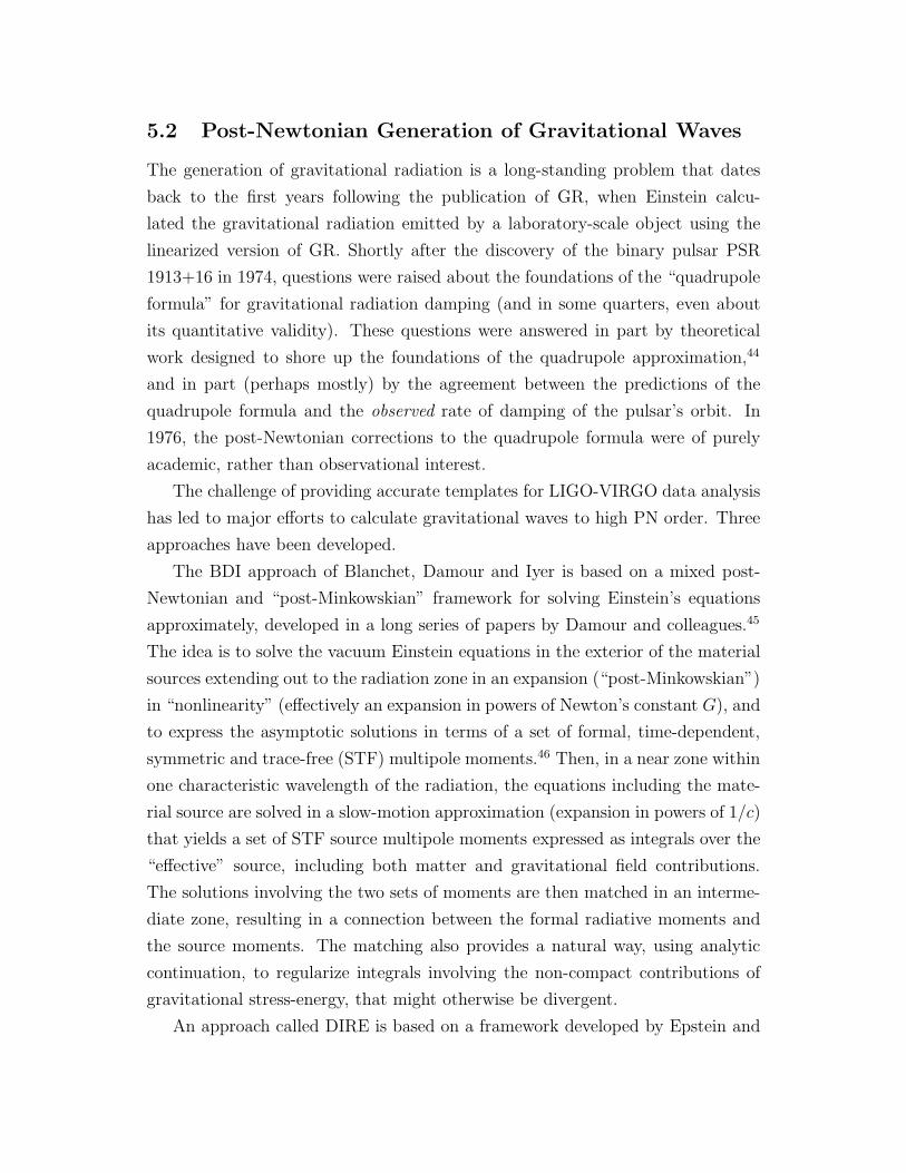
5.2 Post-Newtonian Generation of Gravitational Waves
The generation of gravitational radiation is a long-standing problem that dates
back to the first years following the publication of GR, when Einstein calcu-
lated the gravitational radiation emitted by a laboratory-scale object using the
linearized version of GR. Shortly after the discovery of the binary pulsar PSR
1913+16 in 1974, questions were raised about the foundations of the “quadrupole
formula” for gravitational radiation damping (and in some quarters, even about
its quantitative validity). These questions were answered in part by theoretical
work designed to shore up the foundations of the quadrupole approximation,44
and in part (perhaps mostly) by the agreement between the predictions of the
quadrupole formula and the observed rate of damping of the pulsar’s orbit. In
1976, the post-Newtonian corrections to the quadrupole formula were of purely
academic, rather than observational interest.
The challenge of providing accurate templates for LIGO-VIRGO data analysis
has led to major efforts to calculate gravitational waves to high PN order. Three
approaches have been developed.
The BDI approach of Blanchet, Damour and Iyer is based on a mixed post-
Newtonian and “post-Minkowskian” framework for solving Einstein’s equations
approximately, developed in a long series of papers by Damour and colleagues.45
The idea is to solve the vacuum Einstein equations in the exterior of the material
sources extending out to the radiation zone in an expansion (“post-Minkowskian”)
in “nonlinearity” (effectively an expansion in powers of Newton’s constant G), and
to express the asymptotic solutions in terms of a set of formal, time-dependent,
symmetric and trace-free (STF) multipole moments.46 Then, in a near zone within
one characteristic wavelength of the radiation, the equations including the mate-
rial source are solved in a slow-motion approximation (expansion in powers of 1/c)
that yields a set of STF source multipole moments expressed as integrals over the
“effective” source, including both matter and gravitational field contributions.
The solutions involving the two sets of moments are then matched in an interme-
diate zone, resulting in a connection between the formal radiative moments and
the source moments. The matching also provides a natural way, using analytic
continuation, to regularize integrals involving the non-compact contributions of
gravitational stress-energy, that might otherwise be divergent.
An approach called DIRE is based on a framework developed by Epstein and

Wagoner (EW),47 and extended by Will, Wiseman and Pati. We shall describe
DIRE briefly below.
A third approach, valid only in the limit in which one mass is much smaller
than the other, is that of black-hole perturbation theory. This method provides
numerical results that are exact in v/c, as well as analytical results expressed as
series in powers of v/c, both for non-rotating and for rotating black holes. For
non-rotating holes, the analytical expansions have been carried to 5.5 PN order.48
In all cases of suitable overlap, the results of all three methods agree precisely.
5.2.1 Direct Integration of the Relaxed Einstein Equations (DIRE)
Like the BDI approach, DIRE involves rewriting the Einstein equations in their
“relaxed” form, namely as an inhomogeneous, flat-spacetime wave equation for a
field hαβ , whose formal solution can be written
hαβ(t,x) = 4∫
C
ταβ(t− |x − x′|,x′)
|x− x′| d3x′ . (69)
where the source ταβ consists of both the material stress-energy, and a “gravita-
tional stress-energy” made up of all the terms non-linear in hαβ , and the integra-
tion is over the past flat-spacetime null-cone C of the field point (t,x) (see Fig.
7). The wave equation is accompanied by a harmonic or deDonder gauge con-
dition hαβ ,β = 0, which serves to specify a coordinate system, and also imposes
equations of motion on the sources. Unlike the BDI approach, a single formal
solution is written down, valid everywhere in spacetime. This formal solution, is
then iterated in a slow-motion (v/c < 1), weak-field (||hαβ|| < 1 ) approximation,
that is very similar to the corresponding procedure in electromagnetism. However,
because the integrand of this retarded integral is not compact by virture of the
non-linear field contributions, the original EW formalism quickly runs up against
integrals that are not well defined, or worse, are divergent. Although at the low-
est quadrupole and first few PN orders, various arguments can be given to justify
sweeping such problems under the rug,49 they are not very rigorous, and provide
no guarantee that the divergences do not become insurmountable at higher orders.
As a consequence, despite efforts to cure the problem, the EW formalism fell into
some disfavor as a route to higher orders, although an extension to 3/2PN order
was accomplished.50
The resolution of this problem involves taking literally the statement that the

Field point (t,x)
Matter source
C − N
CD
N
Fig. 7. Past harmonic null cone C of the field point (t,x) intersects the near zone
D in the hypersurface N .
D
MN
(t,x)
t−r
AAAAAAAAAAAAAAAAAAAAAAAAAAAAAAAAAAAAAAAAAAAAAAAAAAAAAAAAAAAAAAAAAAAAAAAAAAA
Fig. 8. Taylor expansion of retarded time dependence on N results in multi-
pole moments integrated over the spatial hypersurface M, corresponding to fixed
retarded time t− r
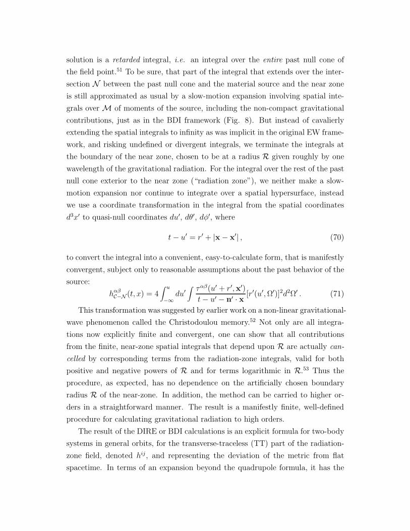
solution is a retarded integral, i.e. an integral over the entire past null cone of
the field point.51 To be sure, that part of the integral that extends over the inter-
section N between the past null cone and the material source and the near zone
is still approximated as usual by a slow-motion expansion involving spatial inte-
grals over M of moments of the source, including the non-compact gravitational
contributions, just as in the BDI framework (Fig. 8). But instead of cavalierly
extending the spatial integrals to infinity as was implicit in the original EW frame-
work, and risking undefined or divergent integrals, we terminate the integrals at
the boundary of the near zone, chosen to be at a radius R given roughly by one
wavelength of the gravitational radiation. For the integral over the rest of the past
null cone exterior to the near zone (“radiation zone”), we neither make a slow-
motion expansion nor continue to integrate over a spatial hypersurface, instead
we use a coordinate transformation in the integral from the spatial coordinates
d3x′ to quasi-null coordinates du′, dθ′, dφ′, where
t− u′ = r′ + |x − x′| , (70)
to convert the integral into a convenient, easy-to-calculate form, that is manifestly
convergent, subject only to reasonable assumptions about the past behavior of the
source:
hαβC−N (t, x) = 4
∫ u
−∞du′
∫
ταβ(u′ + r′,x′)
t− u′ − n′ · x [r′(u′,Ω′)]2d2Ω′ . (71)
This transformation was suggested by earlier work on a non-linear gravitational-
wave phenomenon called the Christodoulou memory.52 Not only are all integra-
tions now explicitly finite and convergent, one can show that all contributions
from the finite, near-zone spatial integrals that depend upon R are actually can-
celled by corresponding terms from the radiation-zone integrals, valid for both
positive and negative powers of R and for terms logarithmic in R.53 Thus the
procedure, as expected, has no dependence on the artificially chosen boundary
radius R of the near-zone. In addition, the method can be carried to higher or-
ders in a straightforward manner. The result is a manifestly finite, well-defined
procedure for calculating gravitational radiation to high orders.
The result of the DIRE or BDI calculations is an explicit formula for two-body
systems in general orbits, for the transverse-traceless (TT) part of the radiation-
zone field, denoted hij , and representing the deviation of the metric from flat
spacetime. In terms of an expansion beyond the quadrupole formula, it has the

schematic form,
hij =2Gµ
R
Qij [1 +O(ǫ1/2) +O(ǫ) +O(ǫ3/2) +O(ǫ2) . . .]
TT, (72)
where µ is the reduced mass, R is the distance to the source, and Qij represents
two time derivatives of the mass quadrupole moment tensor (the series actually
contains multipole orders beyond quadrupole). The expansion parameter ǫ is
related to the orbital variables by ǫ ∼ m/r ∼ v2, where r is the distance be-
tween the bodies, v is the relative velocity, and m = m1 + m2 is the total mass
(G = c = 1). The 1/2PN and 1PN terms were derived by Wagoner and Will,49
the 3/2PN terms by Wiseman.50 The contribution of gravitational-wave “tails”,
caused by backscatter of the outgoing radiation off the background spacetime cur-
vature, at O(ǫ3/2), were derived and studied by several authors. The 2PN terms
including 2PN tail contributions were derived by two independent groups and are
in complete agreement (see Refs. 51,54 for details and references to earlier work).
There are also contributions to the waveform due to intrinsic spin of the bod-
ies, which occur at O(ǫ3/2) (spin-orbit) and O(ǫ2) (spin-spin); these have been
calculated elsewhere.55
Given the gravitational waveform, one can compute the rate at which energy
is carried off by the radiation (schematically∫
hhdΩ, the gravitational analog of
the Poynting flux). For the special case of non-spinning bodies moving on quasi-
circular orbits (i.e. circular apart from a slow inspiral), the energy flux through
2PN order has the form
dE
dt=
32
5η2(
m
r
)5[
1 − m
r
(
2927
336+
5
4η)
+4π(
m
r
)3/2
+(
m
r
)2 (293383
9072+
380
9η)]
, (73)
where η = m1m2/m2. The first term is the quadrupole contribution, the second
term is the 1PN contribution, the third term, with the coefficient 4π, is the “tail”
contribution, and the fourth term is the 2PN contribution first reported jointly
by Blanchet et al.56 Calculation of the 3PN contributions is nearing completion.
Similar expressions can be derived for the loss of angular momentum and
linear momentum. These losses react back on the orbit to circularize it and
cause it to inspiral. The result is that the orbital phase (and consequently the
gravitational-wave phase) evolves non-linearly with time. It is the sensitivity of
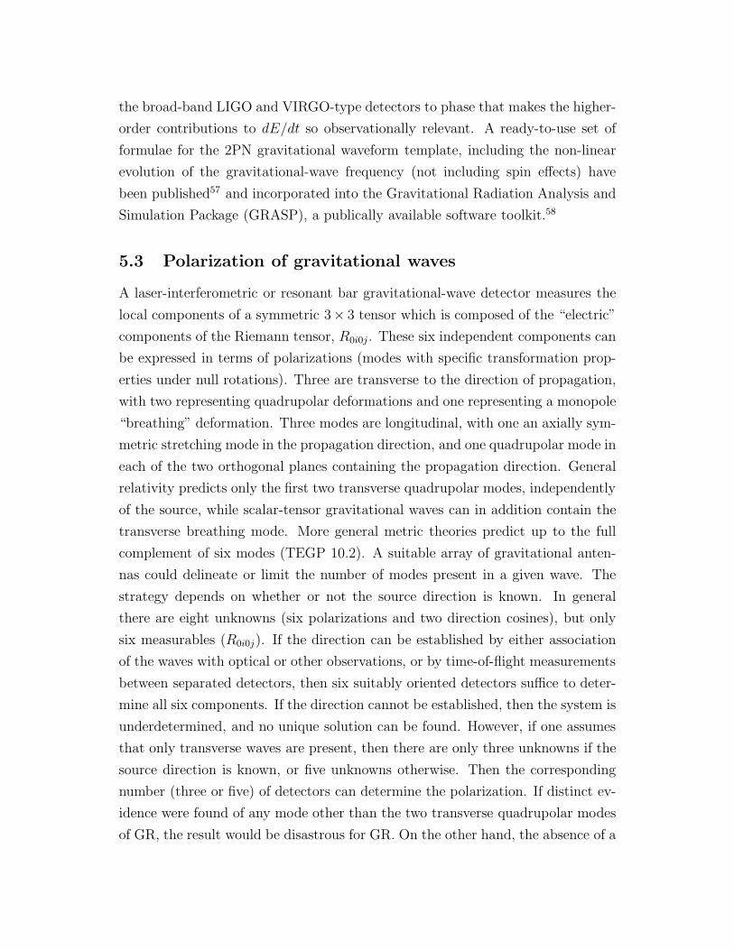
the broad-band LIGO and VIRGO-type detectors to phase that makes the higher-
order contributions to dE/dt so observationally relevant. A ready-to-use set of
formulae for the 2PN gravitational waveform template, including the non-linear
evolution of the gravitational-wave frequency (not including spin effects) have
been published57 and incorporated into the Gravitational Radiation Analysis and
Simulation Package (GRASP), a publically available software toolkit.58
5.3 Polarization of gravitational waves
A laser-interferometric or resonant bar gravitational-wave detector measures the
local components of a symmetric 3× 3 tensor which is composed of the “electric”
components of the Riemann tensor, R0i0j . These six independent components can
be expressed in terms of polarizations (modes with specific transformation prop-
erties under null rotations). Three are transverse to the direction of propagation,
with two representing quadrupolar deformations and one representing a monopole
“breathing” deformation. Three modes are longitudinal, with one an axially sym-
metric stretching mode in the propagation direction, and one quadrupolar mode in
each of the two orthogonal planes containing the propagation direction. General
relativity predicts only the first two transverse quadrupolar modes, independently
of the source, while scalar-tensor gravitational waves can in addition contain the
transverse breathing mode. More general metric theories predict up to the full
complement of six modes (TEGP 10.2). A suitable array of gravitational anten-
nas could delineate or limit the number of modes present in a given wave. The
strategy depends on whether or not the source direction is known. In general
there are eight unknowns (six polarizations and two direction cosines), but only
six measurables (R0i0j). If the direction can be established by either association
of the waves with optical or other observations, or by time-of-flight measurements
between separated detectors, then six suitably oriented detectors suffice to deter-
mine all six components. If the direction cannot be established, then the system is
underdetermined, and no unique solution can be found. However, if one assumes
that only transverse waves are present, then there are only three unknowns if the
source direction is known, or five unknowns otherwise. Then the corresponding
number (three or five) of detectors can determine the polarization. If distinct ev-
idence were found of any mode other than the two transverse quadrupolar modes
of GR, the result would be disastrous for GR. On the other hand, the absence of a

breathing mode would not necessarily rule out scalar-tensor gravity, because the
strength of that mode depends on the nature of the source.
Although some of the details of implementing such polarization observations
have been worked out for arrays of resonant cylindrical, disk-shaped, and spher-
ical detectors (TEGP 10.2, Ref. 59) only initial work has been done to as-
sess whether the ground-based laser-interferometers (LIGO, VIRGO, GEO600,
TAMA300) could perform interesting polarization measurements. The results de-
pend sensitively on the relative orientation of the detectors’ arms, which are now
cast (literally) in concrete.
5.4 Speed of gravitational waves
According to GR, in the limit in which the wavelength of gravitational waves is
small compared to the radius of curvature of the background spacetime, the waves
propagate along null geodesics of the background spacetime, i.e. they have the
same speed, c, as light (henceforth, we do not set c = 1). In other theories, the
speed could differ from c because of coupling of gravitation to “background” grav-
itational fields. For example, in the Rosen bimetric theory with a flat background
metric η, gravitational waves follow null geodesics of η, while light follows null
geodesics of g (TEGP 10.1).
Another way in which the speed of gravitational waves could differ from c is
if gravitation were propagated by a massive field (a massive graviton), in which
case, vg would be given by, in a local inertial frame,
v2g
c2= 1 − m2
gc4
E2, (74)
where mg and E are the graviton rest mass and energy, respectively. For a recent
review of the idea of a massive graviton see Ref. 60.
The most obvious way to test this is to compare the arrival times of a gravita-
tional wave and an electromagnetic wave from the same event, e.g. a supernova.
For a source at a distance D, the resulting value of the difference 1 − vg/c is
1 − vg
c= 5 × 10⁻¹⁷
(
200Mpc
D
)(
∆t
1s
)
, (75)
where ∆t ≡ ∆ta − (1+Z)∆te is the “time difference”, where ∆ta and ∆te are the
differences in arrival time and emission time, respectively, of the two signals, and
Z is the redshift of the source. In many cases, ∆te is unknown, so that the best

x
y
x
y
z
x
z
y
x
y
z
y
(b)
(d)
(f)(e)
(c)
(a)
GR = ST = +
Fig. 9. Six polarization modes for gravitational waves permitted in any metric
theory of gravity. Shown is the displacement that each mode induces on a ring of
test particles. The wave propagates in the +z direction. There is no displacement
out of the plane of the picture. In (a), (b) and (c), the wave propagates out of the
plane; in (d), (e), and (f), the wave propagates in the plane. In general relativity,
only (a) and (b) are present; in scalar-tensor gravity, (c) may also be present.
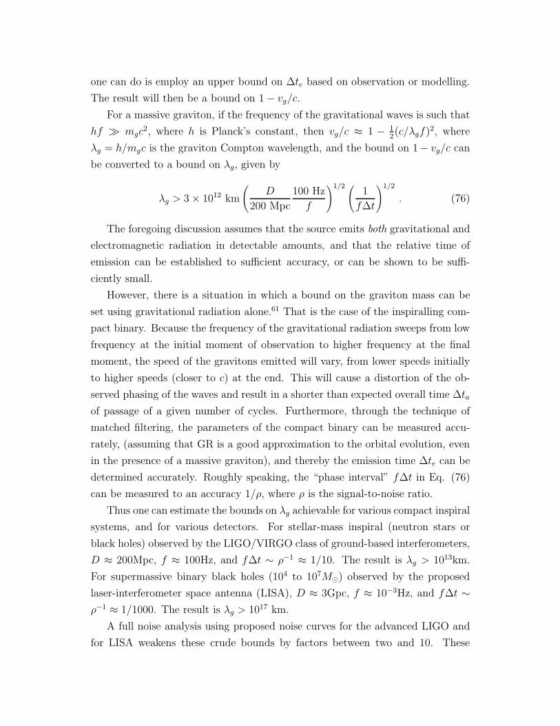
one can do is employ an upper bound on ∆te based on observation or modelling.
The result will then be a bound on 1 − vg/c.
For a massive graviton, if the frequency of the gravitational waves is such that
hf ≫ mgc2, where h is Planck’s constant, then vg/c ≈ 1 − 1
2(c/λgf)2, where
λg = h/mgc is the graviton Compton wavelength, and the bound on 1− vg/c can
be converted to a bound on λg, given by
λg > 3 × 10¹² km
(
D
200 Mpc
100 Hz
f
)1/2 (1
f∆t
)1/2
. (76)
The foregoing discussion assumes that the source emits both gravitational and
electromagnetic radiation in detectable amounts, and that the relative time of
emission can be established to sufficient accuracy, or can be shown to be suffi-
ciently small.
However, there is a situation in which a bound on the graviton mass can be
set using gravitational radiation alone.61 That is the case of the inspiralling com-
pact binary. Because the frequency of the gravitational radiation sweeps from low
frequency at the initial moment of observation to higher frequency at the final
moment, the speed of the gravitons emitted will vary, from lower speeds initially
to higher speeds (closer to c) at the end. This will cause a distortion of the ob-
served phasing of the waves and result in a shorter than expected overall time ∆ta
of passage of a given number of cycles. Furthermore, through the technique of
matched filtering, the parameters of the compact binary can be measured accu-
rately, (assuming that GR is a good approximation to the orbital evolution, even
in the presence of a massive graviton), and thereby the emission time ∆te can be
determined accurately. Roughly speaking, the “phase interval” f∆t in Eq. (76)
can be measured to an accuracy 1/ρ, where ρ is the signal-to-noise ratio.
Thus one can estimate the bounds on λg achievable for various compact inspiral
systems, and for various detectors. For stellar-mass inspiral (neutron stars or
black holes) observed by the LIGO/VIRGO class of ground-based interferometers,
D ≈ 200Mpc, f ≈ 100Hz, and f∆t ∼ ρ−1 ≈ 1/10. The result is λg > 1013km.
For supermassive binary black holes (104 to 107M⊙) observed by the proposed
laser-interferometer space antenna (LISA), D ≈ 3Gpc, f ≈ 10−3Hz, and f∆t ∼ρ−1 ≈ 1/1000. The result is λg > 1017 km.
A full noise analysis using proposed noise curves for the advanced LIGO and
for LISA weakens these crude bounds by factors between two and 10. These

potential bounds can be compared with the solid bound λg > 2.8×10¹² km, derived
from solar system dynamics, which limit the presence of a Yukawa modification
of Newtonian gravity of the form V (r) = (GM/r) exp(−r/λg),62 and with the
model-dependent bound λg > 6 × 10¹⁹ km from consideration of galactic and
cluster dynamics.60
5.5 Gravitational Radiation Back-reaction
This plays an important role only in the inspiral of compact objects. The equa-
tions of motion of inspiral include the non-radiative, non-linear post-Newtonian
corrections of Newtonian motion, as well as radiation back-reaction and its non-
linear post-Newtonian corrections. The evolution of the orbit is imprinted on the
phasing of the inspiral waveform, to which broad-band laser interferometers are
especially sensitive through the use of matched filtering of the data against the-
oretical templates derived from GR.63 A number of tests of GR using matched
filtering of binary inspiral have been discussed, including putting a bound on
scalar-tensor gravity,64 measuring the non-linear “tail term” in gravitational ra-
diation damping65 (the “4π” term in Eq. (73)), and testing the GR “no hair”
theorems by mapping spacetime outside black holes.66
For example, the dipole gravitational radiation predicted by scalar-tensor the-
ories results in modifications in gravitational-radiation back-reaction. The effects
are strongest for systems involving a neutron star and a black hole. Double neu-
tron star systems are less promising because the small range of masses available
near 1.4 M⊙ results in suppression of dipole radiation by symmetry. Double black-
hole systems turn out to be observationally identical in the two theories.
For example, for a 1.4 M⊙ neutron star and a 10 M⊙ (3 M⊙) black hole at
200 Mpc, the bound on ωBD could be 600 (1800) (using advanced LIGO noise
curves). The bound increases linearly with signal-to-noise ratio. If one demands
that this test be performed annually, thus requiring observation of frequent, and
therefore more distant, weaker sources, the bounds on ωBD will be too weak to
compete with existing bounds. However, if one is prepared to wait 10 years for
the lucky observation of a nearby, strong source, the resulting bound could exceed
the current bound. The bounds are illustrated in Figure 10 by the curves marked
N = 1 and N = 1/10. Figure 10 assumes a double-neutron-star inspiral rate of
10−6 per year per galaxy, and a black-hole-neutron-star rate β times that, where

N = Number detected per year
β = NS−BH rate/NS−NS rateB
OU
ND
ON
ω
β=10
β=1
β=1β=1/10
N=1
N=1/10
3 4 5 6 7 8 9 10
BLACK HOLE MASS
1000
2000
3000
4000
5000
6000
Fig. 10. Bounds on the scalar-tensor coupling constant ωBD from gravitational-
wave observations of inspiralling black-hole neutron-star systems. The solar sys-
tem bound is around ωBD = 3000.
β is highly uncertain.
6 Conclusions
In 1998 we find that general relativity has held up under extensive experimental
scrutiny. The question then arises, why bother to continue to test it? One reason
is that gravity is a fundamental interaction of nature, and as such requires the
most solid empirical underpinning we can provide. Another is that all attempts
to quantize gravity and to unify it with the other forces suggest that the stan-
dard general relativity of Einstein is not likely to be the last word. Furthermore,
the predictions of general relativity are fixed; the theory contains no adjustable
constants so nothing can be changed. Thus every test of the theory is either a

potentially deadly test or a possible probe for new physics. Although it is remark-
able that this theory, born 80 years ago out of almost pure thought, has managed
to survive every test, the possibility of finding a discrepancy will continue to drive
experiments for years to come.
Acknowledgments
This work was supported in part by the National Science Foundation, Grant
Number PHY 96-00049.
References
[1] C. M. Will Was Einstein Right? 2nd Ed. (Basic Books, New York, 1993).
[2] C. M. Will, Theory and Experiment in Gravitational Physics 2nd Ed. (Cam-
bridge University Press, Cambridge, 1993).
[3] C. M. Will, in 300 Years of Gravitation, edited by S. W. Hawking and W.
Israel, 80–127 (Cambridge University Press, Cambridge, 1987), p. 80.
[4] C. M. Will, Int J. Mod. Phys. D 1, 13 (1992).
[5] C. M. Will, in General Relativity: Proceedings of the 46th Scottish Universities
Summer School in Physics, ed. G. S. Hall and J. R. Pulham (Institute of Physics
Publishing, Bristol, 1996), p. 239.
[6] T. Damour, in Proceedings of the 5th Hellenic School on Elementary Particle
Physics, in press (gr-qc/9606079).
[7] Y. Su, B. R. Heckel, E. G. Adelberger, J. H. Gundlach, M. Harris, G. L. Smith,
and H. E. Swanson, Phys. Rev. D 50, 3614 (1994).
[8] E. Fischbach, G. T. Gillies, D. E. Krause, J. G. Schwan, and C. Talmadge,
Metrologia 29, 213 (1992).
[9] A. Godone, C. Novero, and P. Tavella, Phys. Rev. D 51, 319 (1995).
[10] J. D. Prestage, R. L. Tjoelker, and L. Maleki, Phys. Rev. Lett. 74, 3511
(1995).
[11] F. Dyson and T. Damour, Nucl. Phys. B480, 37 (1996) (hep-ph/9606486).
[12] M. J. Drinkwater, J. K. Webb, J. D. Barrow, and V. V. Flambaum, Mon.
Not. R. Astron. Soc. 295, 457 (1998) (astro-ph/9711290).
[13] R. A. Malaney and G. Mathews, Phys. Rep. 229, 147 (1993); H. Reeves,
Rev. Mod. Phys. 66, 193 (1994).
[14] C. M. Will, Phys. Rev. D 45 403 (1992).
[15] E. Fischbach and C. Talmadge, Nature 356, 207 (1992).
[16] C. M. Will, Sky and Telescope 80, 472 (1990).
[17] E. G. Adelberger, B. R. Heckel, C. W. Stubbs, and W. F. Rogers, Ann. Rev.
Nucl. Particle Sci. 41, 269 (1991).
[18] C. W. Misner, K. S. Thorne, and J. A. Wheeler, Gravitation (Freeman Pub-
lishing Co, San Francisco, 1973).
[19] S. W. Weinberg S W, Gravitation and Cosmology (Wiley, New York, 1992).
[20] T. Damour and G. Esposito-Farese, Class. Quantum Grav. 9, 2093 (1992).
[21] T. Damour and K. Nordtvedt, Phys. Rev. Lett. 70, 2217 (1993); Phys. Rev.
D 48, 3436 (1993).
[22] P. J. Steinhardt and C. M. Will, Phys. Rev. D 52, 628 (1995) (astro-
ph/9409041).
[23] T. Damour and G. Esposito-Farese, Phys.Rev. D 54, 1474 (1996) (gr-
qc/9602056).
[24] T. M. Eubanks, D. N. Matsakis, J. O. Martin, B. A. Archinal, D. D. Mc-
Carthy, S. A. Klioner, S. Shapiro, and I. I. Shapiro, Bull. Am. Phys. Soc.,
Abstract #K 11.05 (1997), unpublished
[25] M. Froeschle, F. Mignard and F. Arenou, in Proceedings of the Hipparcos
Venice 1997 Symposium, in press.
[26] K. Nordtvedt, Icarus 114, 51 (1995).
[27] T. Damour and D. Vokrouhlicky, Phys. Rev. D, 53, 6740 (1996) (gr-
qc/9606076).
[28] J. O. Dickey, P. L. Bender, J. E. Faller, X X Newhall, R. L. Ricklefs, J. G.
Ries, P. J. Shelus, C. Veillet, A. L. Whipple, J. R. Wiant, J. G. Williams, and
C. F. Yoder, Science 265, 482 (1994); J. G. Williams, X X Newhall, and J. O.
Dickey, Phys. Rev. D53, 6730 (1996).
[29] J. F. Bell and T. Damour, Class. Quantum Grav. 13, 3121 (1996) (gr-
qc/9606062).
[30] J. F. Bell, F. Camilo, T. Damour, Astrophys. J. 464, 857 (1996) (astro-
ph/9512100).
[31] C. M. Will, Astrophys J 204, 224 (1976).
[32] C. M. Will, Astrophys J. Lett. 393, L59 (1992).
[33] For information about the project, see http://einstein.stanford.edu/.
[34] I. Ciufolini, E. Pavlis, F. Chieppa, E. Fernandes-Vieira, and J. Pirez-
Mercader, Science 279, 2100 (1998).
[35] K. S. Thorne, in Proceedings of the Snowmass 95 Summer Study on Particle
and Nuclear Astrophysics and Cosmology, edited by E. W. Kolb and R. Peccei
(World Scientific, Singapore, 1995), p. 398 (gr-qc/9506086).
[36] R. A. Hulse, Rev. Mod. Phys. 66, 699 (1994).
[37] J. H. Taylor, Rev. Mod. Phys. 66, 711 (1994).
[38] T. Damour , 1987, in 300 Years of Gravitation, eds Hawking S W and Israel
W, 128–198 (Cambridge University Press, Cambridge).
[39] M. Kramer, Astrophys. J., in press (astro-ph/9808127).
[40] A. Wolszczan, Class. Quantum Grav. 11, A227 (1994).
[41] I. H. Stairs, Z. Arzoumanian, F. Camilio, A. G. Lyne, D. J. Nice, J. H. Taylor,
S. E. Thorsett, and A. Wolszczan, Astrophys. J., in press (astro-ph/9712296).
[42] L. S. Finn and D. F. Chernoff, Phys. Rev. D 47, 2198 (1993) (gr-qc/9301003);
C. Cutler and E. E. Flanagan, Phys. Rev. D 49, 2658 (1994) (gr-qc/9402014);
E. Poisson and C. M. Will, Phys. Rev. D 52, 848 (1995) (gr-qc/9502040).
[43] This convention holds sway, despite the fact that pure Newtonian gravity
predicts no gravitational radiation. It is often the source of confusion, since the
energy carried by the lowest-order “Newtonian” quadrupole radiation manifests
itself in a (post)5/2-Newtonian, orO[(v/c)5] correction in the equation of motion.
[44] M. Walker and C. M. Will, Phys. Rev. Lett. 45, 1741 (1980); J. L. Anderson,
Phys. Rev. Lett. 45, 1745 (1980); T. Damour, Phys. Rev. Lett. 51, 1019 (1983);
D. Christodoulou and B. G. Schmidt, Commun. Math. Phys. 68, 275 (1979); R.
A. Isaacson, J. S. Welling, and J. Winicour, Phys. Rev. Lett. 53, 1870 (1984).

[45] L. Blanchet, T. Damour, Phil. Trans. R. Soc. London A320, 379 (1986); L.
Blanchet and T. Damour, Phys. Rev. D 37, 1410 (1988); L. Blanchet and T.
Damour, Ann. Inst. H. Poincare (Phys. Theorique) 50, 377 (1989); T. Damour
and B. R. Iyer, Ann. Inst. H. Poincare (Phys. Theorique) 54, 115 (1991); L.
Blanchet, Phys. Rev. D 51, 2559 (1995) (gr-qc/9501030); L. Blanchet and T.
Damour, Phys. Rev. D 46, 4304 (1992).
[46] K. S. Thorne, Rev. Mod. Phys. 52, 299 (1980).
[47] R. Epstein and R. V. Wagoner, Astrophys. J. 197, 717 (1975) (EW).
[48] E. Poisson, Phys. Rev. D 47, 1497 (1993); E. Poisson and M. Sasaki, Phys.
Rev. D 51, 5753 (1995) (gr-qc/9412027); C. Cutler, L. S. Finn, E. Poisson, and
G. J. Sussman, Phys. Rev. D 47, 1511 (1993); M. Sasaki, Prog. Theor. Phys.
92, 17 (1994) (gr-qc/9402042); H. Tagoshi and M. Sasaki, Prog. Theor. Phys.
92, 745 (1994) (gr-qc/9405062); T. Tanaka, H. Tagoshi, and M. Sasaki, Prog.
Theor. Phys. 96, 1087 (1996) (gr-qc/9701050).
[49] R. V. Wagoner and C. M. Will, Astrophys. J. 210, 764 (1976).
[50] A. G. Wiseman, Phys. Rev. D 46 1517 (1992).
[51] C. M. Will and A. G. Wiseman, Phys. Rev. D 54, 4813 (1996) (gr-
qc/9608012).
[52] A. G. Wiseman and C. M. Will, Phys. Rev. D 44, R2945 (1991).
[53] C. M. Will and M. E. Pati, papers in preparation.
[54] L. Blanchet, T. Damour, and B. R. Iyer, Phys. Rev. D 51, 5360 (1995) (gr-
qc/9501029).
[55] L. E. Kidder, C. M. Will, and A. G. Wiseman, Phys. Rev. D 47, R4183 (1993)
(gr-qc/9211025); L. E. Kidder, Phys. Rev. D 52, 821 (1995) (gr-qc/9506022).
[56] L. Blanchet, T. Damour, B. R. Iyer, C. M. Will and A. G. Wiseman, Phys.
Rev. Lett. 74, 3515 (1995) (gr-qc/9501027).
[57] L. Blanchet, B. R. Iyer, C. M. Will, and A. G. Wiseman, Class. Quantum
Grav. 13, 575 (1996) (gr-qc/9602024).
[58] See http://www.ligo.caltech.edu/LIGO web/Collaboration/manual.pdf.
[59] J. A. Lobo, Phys. Rev. D52, 591 (1995).
[60] M. Visser, Gen. Relativ. Gravit., in press (gr-qc/9705051).
[61] C. M. Will, Phys. Rev. D57, 2061 (1998) (gr-qc/9709011).
[62] C. Talmadge, J.-P. Berthias, R. W. Hellings, and E. M. Standish, Phys. Rev.
Lett. 61, 1159 (1988).
[63] C. Cutler, T. A. Apostolatos, L. Bildsten, L. S. Finn, E. E. Flanagan, D.
Kennefick, D. M. Markovic, A. Ori, E. Poisson, G. J. Sussman, and K. S.
Thorne, Phys. Rev. Lett. 70, 2984 (1993) (astro-ph/9208005).
[64] C. M. Will, Phys. Rev. D50 6058 (1994) (gr-qc/9406022).
[65] L. Blanchet and B. S. Sathyaprakash, Class. Quantum Grav. 11, 2807 (1994);
Phys. Rev. Lett. 74, 1067 (1995).
[66] F. D. Ryan, Phys. Rev. D52, 5707 (1995); E. Poisson, Phys. Rev. D54, 5939
(1996) (gr-qc/9606024).