the concept of soft channel encoding and its applications ...sc.enseeiht.fr/doc/seminar_matz.pdf ·...
TRANSCRIPT

The Concept of Soft Channel Encoding andits Applications in Wireless Relay Networks
Gerald Matz
Institute of Telecommunications
Vienna University of Technology
institute oftelecommunications
Acknowledgements
People:
• Andreas Winkelbauer
• Clemens Novak
• Stefan Schwandter
Funding:
SISE - Information Networks (FWF Grant S10606)
2

Outline
1. Introduction
2. Soft channel encoding
3. Approximations
4. Applications
5. Conclusions and outlook
3

Outline
1. Introduction
2. Soft channel encoding
3. Approximations
4. Applications
5. Conclusions and outlook
4

Introduction: Basic Idea
Soft information processing
• popular in modern receivers
• idea: use soft information also for transmission
Soft-input soft-output (SISO) encoding
• extension of hard-input hard-output (HIHO) encoding
• data only known in terms of probabilities
• how to (efficiently) encode “noisy” data?
Applications
• physical layer network coding
• distributed (turbo) coding
• joint source-channel coding
5
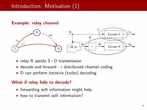
Introduction: Motivation (1)
Example: relay channel
D
xS
xS
xR
R
S
u′
R
πxR
xS
SR ch.
Encoder S
Encoder Ru
uS
• relay R assists S – D transmission
• decode-and-forward → distributed channel coding
• D can perform iterative (turbo) decoding
What if relay fails to decode?
• forwarding soft information might help
• how to transmit soft information?
6
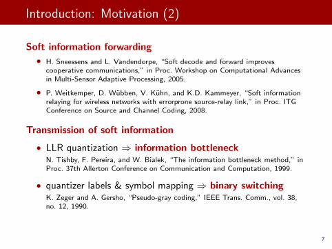
Introduction: Motivation (2)
Soft information forwarding
• H. Sneessens and L. Vandendorpe, “Soft decode and forward improvescooperative communications,” in Proc. Workshop on Computational Advancesin Multi-Sensor Adaptive Processing, 2005.
• P. Weitkemper, D. Wubben, V. Kuhn, and K.D. Kammeyer, “Soft informationrelaying for wireless networks with errorprone source-relay link,” in Proc. ITGConference on Source and Channel Coding, 2008.
Transmission of soft information
• LLR quantization ⇒ information bottleneckN. Tishby, F. Pereira, and W. Bialek, “The information bottleneck method,” inProc. 37th Allerton Conference on Communication and Computation, 1999.
• quantizer labels & symbol mapping ⇒ binary switchingK. Zeger and A. Gersho, “Pseudo-gray coding,” IEEE Trans. Comm., vol. 38,no. 12, 1990.
7

Outline
1. Introduction
2. Soft channel encoding
3. Approximations
4. Applications
5. Conclusions and outlook
8

Hard Encoding/Decoding Revisited
Notation
• information bit sequence: u = (u1 . . . uK)T ∈ {0, 1}K
• code bit sequence: c = (c1 . . . cN )T ∈ {0, 1}N
• assume N ≥ K
Linear binary channel code
• one-to-one mapping φ between data bits u and code bits c
• encoding: c = φ(u)
• codebook: C = φ({0, 1}K
)Hard decoding:
• observed code bit sequence c′ = c⊕ e = φ(u)⊕ e
• decoder: mapping ψ such that ψ(c′) is “close” to u
9

Soft Decoding Revisited
Word-level
• observations: code bit sequence probabilities pin(c′)
• enforce code constraint:
p′(c) =
{pin(c)∑
c′∈C pin(c′) , c ∈ C
0, else
• info bit sequence probabilities: pout(u) = p′(φ(u))• conceptually simple, computationally infeasible
Bit-level
• observed: code bit probabilities pin(cn) =∑∼cn
pin(c′)
• desired: info bit probabilities pout(uk) =∑∼uk
pout(φ(u))
• conceptually more difficult, computationally feasible
• example: equivalent to BCJR for convolutional codes
10
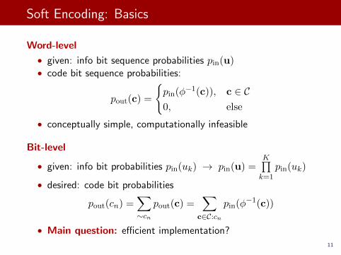
Soft Encoding: Basics
Word-level
• given: info bit sequence probabilities pin(u)• code bit sequence probabilities:
pout(c) =
{pin(φ
−1(c)), c ∈ C0, else
• conceptually simple, computationally infeasible
Bit-level
• given: info bit probabilities pin(uk) → pin(u) =K∏k=1
pin(uk)
• desired: code bit probabilities
pout(cn) =∑∼cn
pout(c) =∑
c∈C:cnpin(φ
−1(c))
• Main question: efficient implementation?11

Soft Encoding: LLRs
System model: SISO
encoder
binary
source
noisy binary source
u L(u) L(c|u)channel
noisy
Log-likelihood ratios (LLR)
• definition:
L(uk) = logpin(uk=0)
pin(uk=1), L(cn) = log
pout(cn=0)
pout(cn=1)
• encoder input: L(u) = (L(u1) . . . L(uK))T
• encoder output: L(c) = (L(c1) . . . L(cN ))T
12
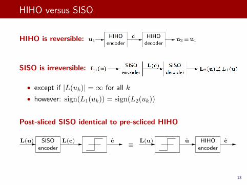
HIHO versus SISO
HIHO is reversible:
SISO is irreversible:
• except if |L(uk)| =∞ for all k
• however: sign(L1(uk)) = sign(L2(uk))
Post-sliced SISO identical to pre-scliced HIHO
SISO
encoder
L(u) c cHIHO
encoder
uL(u)≡
L(c)
13

Block Codes (1)
Binary (N,K) block code C with generator matrix G ∈ FN×K2
HIHO encoding: c = Gu, involves XOR/modulo 2 sum ⊕
Statistics of XOR:
p(uk⊕ul=0) = p(uk=0)p(ul=0) + p(uk=1)p(ul=1)
Boxplus: L(uk⊕ul) , L(uk)� L(ul) = 1 + eL(uk)+L(ul)
eL(uk) + eL(ul)
• � is associative and commutative
• |L1 � L2| ≤ min{|L1|, |L2|}
J. Hagenauer, E. Offer, and L. Papke, “Iterative decoding of binary block and
convolutional codes,” IEEE Trans. Inf. Theory, vol. 42, no. 2, Feb. 1996.
SISO encoder: replace “⊕” in HIHO encoder by “�”
14

Block Codes (2)
Example: systematic (5, 3) block codec1c2c3c4c5
︸ ︷︷ ︸
c
=
1 0 00 1 00 0 11 1 00 1 1
︸ ︷︷ ︸
G
u1u2u3
︸ ︷︷ ︸
u
=
u1u2u3
u1 ⊕ u2u2 ⊕ u3
L(u1) L(u3)L(u2)
�L(c4)
L(c3)
L(c2)
L(c1)
�L(c5)
u1 u3u2
⊕
⊕
c1
c2
c3
c4
c5
15

Soft Encoding: Convolutional Codes (1)
• Code C with given trellis: use BCJR algorithm
· · ·
· · ·
· · ·
· · ·(1, 1)
(1, 0)
(0, 1)
(0, 0)0
1
2
3
m(m(1),m(0)
)
k = 0 21 3 TT − 3 T − 2 T − 1
αk(m) βk(m)
γk(m′,m) = P
{Sk+1 = m|Sk = m′
}αk(m) =
∑M−1m′=0
αk−1(m′)γk−1(m
′,m)
βk(m) =∑M−1
m′=0βk+1(m
′)γk(m,m′)
pb(c(j)k
)=∑
(m′,m)∈A(j)b
αk(m′)γk(m
′,m)βk+1(m)
A. Winkelbauer and G. Matz, “On efficient soft-input soft-output encoding ofconvolutional codes,” in Proc. ICASSP 2011
16

Soft Encoding: Convolutional Codes (2)
• Observe: only 2 transition probabilites per time instantI Backward recursion βk(m) is rendered superfluous
· · ·
· · ·
· · ·
· · ·(1, 1)
(1, 0)
(0, 1)
(0, 0)0
1
2
3
m(m(1),m(0)
)
k = 0 21 3 TT − 3 T − 2 T − 1
αk(m) βk(m)
• Simplified forward recursion encoder (FRE), reducesI computational complexityI memory requirementsI encoding delay
sk+1(m) =∑
m′∈Bmsk(m
′)γk(m′,m)
pb(c(j)k
)=∑
(m′,m)∈A(j)b
sk(m′)γk(m
′,m)
17

Soft Encoding: Convolutional Codes (2)
• Observe: only 2 transition probabilites per time instantI Backward recursion βk(m) is rendered superfluous
· · ·
· · ·
· · ·
· · ·(1, 1)
(1, 0)
(0, 1)
(0, 0)0
1
2
3
m(m(1),m(0)
)
k = 0 21 3 TT − 3 T − 2 T − 1
αk(m) βk(m)
• Simplified forward recursion encoder (FRE), reducesI computational complexityI memory requirementsI encoding delay
sk+1(m) =∑
m′∈Bmsk(m
′)γk(m′,m)
pb(c(j)k
)=∑
(m′,m)∈A(j)b
sk(m′)γk(m
′,m)17

Soft Encoding: Convolutional Codes (3)
• Special case: non-recursive shift register encoder (SRE)I soft encoder with shift register implementationI linear complexity with minimal memory requirements
• Example: (7, 5)8 convolutional code
DD
L(c2k+1)
L(c2k)
L(uk)
BCJR
operationsper
unittime
constraint length ν
SRE (upper bound)
FRE
2 4 6 8 100
200
400
600
800
1000
18
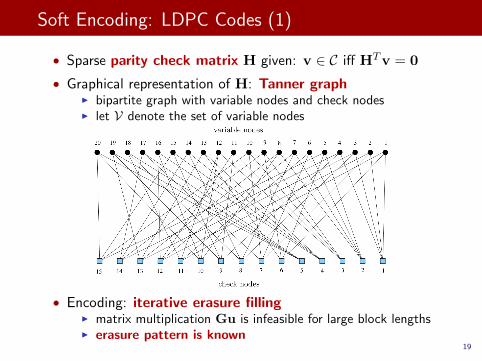
Soft Encoding: LDPC Codes (1)
• Sparse parity check matrix H given: v ∈ C iff HTv = 0
• Graphical representation of H: Tanner graphI bipartite graph with variable nodes and check nodesI let V denote the set of variable nodes
• Encoding: iterative erasure fillingI matrix multiplication Gu is infeasible for large block lengthsI erasure pattern is known
19

Soft Encoding: First Approach
Consider systematic code: c = (uT pT )T
Erasure channel: L(c) = (L(u)T L(p)T )T 7→ (L(u)T 0T )T
deterministic
erasure channel
(L(u)TL(p)T )T
(L(u)TL(p)T )T (L(u)T 0T )T
SISO encoding = decoding ...
• for the erasure channel (erasure filling) or, equivalently,
• w/o channel observation, but with prior soft information on u
Consider special problem structure
• yields efficient implementation
• (much) less complex than SISO decoding
• adjustable accuracy/complexity trade-off
20
Soft Encoding: LDPC Codes (2)
• Iterative erasure filling algorithm1. find all check nodes involving a single erasure2. fill the erasures found in step 13. repeat steps 1-2 until there are no more (recoverable) erasures
• Encoding example:
• Problem: stopping sets ⇒ non-recoverable erasures
21

Soft Encoding: LDPC Codes (2)
• Iterative erasure filling algorithm1. find all check nodes involving a single erasure2. fill the erasures found in step 13. repeat steps 1-2 until there are no more (recoverable) erasures
• Encoding example:
• Problem: stopping sets ⇒ non-recoverable erasures
21
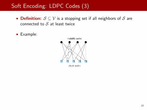
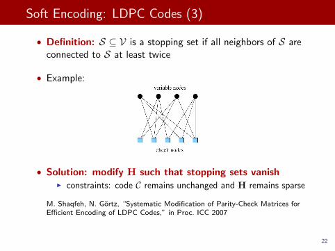
Soft Encoding: LDPC Codes (3)
• Definition: S ⊆ V is a stopping set if all neighbors of S areconnected to S at least twice
• Example:
• Solution: modify H such that stopping sets vanishI constraints: code C remains unchanged and H remains sparse
M. Shaqfeh, N. Gortz, “Systematic Modification of Parity-Check Matrices forEfficient Encoding of LDPC Codes,” in Proc. ICC 2007
22

Outline
1. Introduction
2. Soft channel encoding
3. Approximations
4. Applications
5. Conclusions and outlook
23

Approximations: Boxplus Operator
• Boxplus operator is used frequently in SISO encoding
I Recall a� b = 1 + ea+b
ea + eb
• Approximation: a� b ≈ a � b = sign(a)sign(b)min(|a|, |b|)I small error if
∣∣|a| − |b|∣∣ large
I overestimates true result: a � b ≥ a� bI suitable for hardware implementation
• Correction termsI a� b = a � b+ log(1 + e−|a+b|)− log(1 + e−|a−b|)︸ ︷︷ ︸
− log(2) ≤ additivecorrection ≤ 0
I a� b = a � b ·
(1− 1
min(|a|, |b|)log
1 + e−||a|−|b||
1 + e−||a|+|b||
)︸ ︷︷ ︸
0 ≤ multiplicativecorrection ≤ 1
I Store correction term in (small) lookup table
• Decrease lookup table size by LLR clipping
24

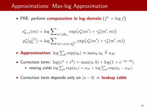
Approximations: Max-log Approximation
• FRE: perform computation in log-domain (f∗ = log f)
s∗k+1(m) = log∑
m′∈Bmexp(s∗k(m
′) + γ∗k(m′,m)
)p∗b(y(j)k
)= log
∑(m′,m)∈A(j)
b
exp(s∗k(m
′) + γ∗k(m′,m)
)• Approximation: log
∑k exp(ak) ≈ maxk ak , aM
• Correction term: log(ea + eb) = max(a, b) + log(1 + e−|a−b|)I nesting yields log
∑k exp(ak) = aM + log
∑k exp(ak − aM )
• Correction term depends only on |a− b| ⇒ lookup table
25

Outline
1. Introduction
2. Soft channel encoding
3. Approximations
4. Applications
5. Conclusions and outlook
26

Applications: Soft Re-encoding (1)
• Soft network coding (NC) for the two-way relay channelI users A and B exchange independent messagesI relay R performs network coding with soft re-encoding
A B
RxR xRR
BA
xBxB
A B
R
xA
xA
• Transmission of quantized soft information is critical
A. Winkelbauer and G. Matz, “Soft-Information-Based Joint Network-Channel Codingfor the Two-Way Relay Channel,” submitted to NETCOD 2011
27

Applications: Soft Re-encoding (1)
• Soft network coding (NC) for the two-way relay channelI users A and B exchange independent messagesI relay R performs network coding with soft re-encoding
A B
RxR xRR
BA
xBxB
A B
R
xA
xA
Puncturer
Puncturerπ
π
Demapperencoder
SISOencoder
Network
encoderModulatorQ(·)
SISOSISOdecoder
SISOdecoder
Demapper
yBR
yAR
xR
• Transmission of quantized soft information is critical
A. Winkelbauer and G. Matz, “Soft-Information-Based Joint Network-Channel Codingfor the Two-Way Relay Channel,” submitted to NETCOD 2011
27

Applications: Soft Re-encoding (2)
• BER simulation resultsI sym. channel conditions, R halfway between A, B, rate 1 bpcu,
256 info bits, 4 level quantization, 1 decoder iteration
soft NC
hard NC
PCCC (5 it.)
BER
γAB [dB]
−8 −6 −4 −2 0 2 4 6
10−5
10−4
10−3
10−2
10−1
100
• SNR gain of ∼ 4.5dB at BER ≈ 10−3 over hard NC28
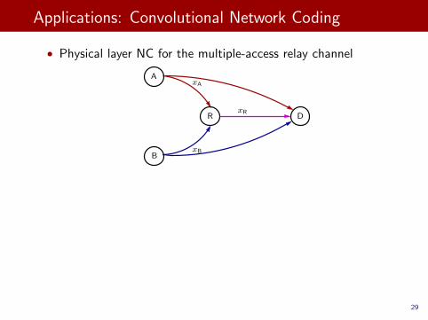
Applications: Convolutional Network Coding
• Physical layer NC for the multiple-access relay channel
xR
xA
xBB
A
R D
• NC at relay
SISO
encoder
L(cA)
L(cB)
LR
L(cA)
L(cB)
LRcR
convolutional NCsoft NChard NC
�⊕cB
cA
29

Applications: Convolutional Network Coding
• Physical layer NC for the multiple-access relay channel
xR
xA
xBB
A
R D
• NC at relay
SISO
encoder
L(cA)
L(cB)
LR
L(cA)
L(cB)
LRcR
convolutional NCsoft NChard NC
�⊕cB
cA
29

Outline
1. Introduction
2. Soft channel encoding
3. Approximations
4. Applications
5. Conclusions and outlook
30

Conclusions and Outlook
Conclusions:
• Efficient methods for soft encoding
• Approximations facilitate practical implementation
• Applications show usefulness of soft encoding
Outlook:
• Frequency domain soft encoding
• Code and transceiver design for physical layer NC
• Performance analysis of physical layer NC schemes
Thank you!
31