the computational complexity of densest region detection

22

⁄0022-0000/02 $35.00© 2002 Elsevier Science (USA)All rights reserved.

Journal of Computer and System Sciences 64, 22–47 (2002)doi:10.1006/jcss.2001.1797, available online at http://www.idealibrary.com on

The Computational Complexity of DensestRegion Detection

Shai Ben-David and Nadav Eiron

Department of Computer Science, Technion, Haifa 32000, IsraelE-mail: [email protected], [email protected]

and

Hans Ulrich Simon

Fakultät für Mathematik, Ruhr Universität Bochum, D-44780 Bochum, GermanyE-mail: [email protected]

Received September 28, 2000; revised March 6, 2001

We investigate the computational complexity of the task of detecting denseregions of an unknown distribution from unlabeled samples of this distribu-tion. We introduce a formal learning model for this task that uses a hypoth-esis class as it ‘‘anti-overfitting’’ mechanism. The learning task in our modelcan be reduced to a combinatorial optimization problem. We can show thatfor some constants, depending on the hypothesis class, these problems areNP-hard to approximate to within these constant factors. We go on andintroduce a new criterion for the success of approximate optimization geo-metric problems. The new criterion requires that the algorithm competes withhypotheses only on the points that are separated by some margin m from theirboundaries. Quite surprisingly, we discover that for each of the two hypoth-esis classes that we investigate, there is a ‘‘critical value’’ of the marginparameter m. For any value below the critical value the problems areNP-hard to approximate, while, once this value is exceeded, the problemsbecome poly-time solvable. © 2002 Elsevier Science (USA)

1. INTRODUCTION

Unsupervised learning is an important area of practical machine learning. Justthe same, the computational learning theory literature has hardly addressed thisissue. Part of this discrepancy may be due to the fact that there is no formal welldefined model that captures the many different tasks that fall into this category.While the formation of such a comprehensive model may be a very difficult task, itsabsence should not deter the COLT community from researching models that

capture restricted subareas of unsupervised learning. In this paper we investigatethe computational complexity aspects of a formal model that addresses one specifictask in this domain.

The model we discuss addresses the problem of locating the densest sub-domainsof a distribution on the basis of seeing random samples generated by that distribu-tion. This is, undoubtedly, one of the applicable tasks of unsupervised learning.

The scenario that we address is one in which the learner is supposed to inferinformation about an unknown distribution from a random sample it generates. Anadequate model should therefore include some mechanism for avoiding over-fitting.That is, the model should impose some restrictions on the class of possible learner’soutputs. The model we propose fixes a collection of domain subsets (a hypothesisclass, if you wish) ahead of seeing the data. The task of the learner is to find amember of this class in which the average density of the example-generating distri-bution is maximized. For simplicity we restrict our attention to the case that thedomain is the Euclidean space Rn. Density is defined relative to the Euclideanvolume. By restricting our hypothesis classes to classes in which all the sets have thesame volume, we can ignore the volume issue.

A model similar to ours was introduced by Ben-David and Lindenbaum [3]. Inthat paper a somewhat more general learning task is considered: given a thresholdr ¥ [0, 1], the learner is required to output the hypothesis in the class that bestapproximates the area on which the distribution has density above r. Ben-Davidand Lindenbaum define a notion of a cost of a hypothesis, relative to a target dis-tribution, and prove (e, d) type generalization bounds. As can be expected, thesample size needed for generalization depends on the VC-dimension of the underly-ing hypothesis class. We refer to that paper for a discussion of the relevance andpotential applications of the model. However, [3] does not address the computa-tional complexity of learning in this model.

Standard uniform convergence considerations imply that detecting a hypothesis(domain subset from the hypothesis class) with close-to-maximal density is essen-tially equivalent to detecting a hypothesis that approximates the maximal empiricaldensity, with respect to the training data. We are therefore led to the following,purely combinatorial, problem:

Given a collection H of subsets of some domain set, on input—a finitesubset P of the domain—output a set h ¥H that maximizes |P 5 h|.

We consider two hypothesis classes: the class of axis aligned hypercubes and theclass of balls (both in Rn). For each of these classes we prove that there exists somec > 0 (independent of the input sample size and dimensionality) such that, unlessP=NP, no polynomial time algorithm can output, for every input sample, ahypothesis in the class that has agreement rate (on the input) within a factor of c ofthe optimal hypothesis in the class.

On the other hand, we consider a relaxation of the common success criterion ofoptimization or approximation algorithms. Rather than requiring an approxima-tion algorithm to achieve a fixed success ratio over all inputs (or over all inputs ofthe same size or dimensionality), we let the required approximation ratio depend on

DENSEST REGION DETECTION 23

the structure of each specific input. Given a hypothesis class H of subsets of 1n Rn,and a parameter m > 0,

an algorithm solves the m-relaxed problem associated with H, if, forevery input sample, it outputs a member of H that contains as manysample points as any member of H can contain with margin \ m (wherethe margin of a point relative to a hypothesis is the radius of the largestball around the point that is fully contained in the hypothesis).

In other words, such an algorithm is required to output a hypothesis with close-to-optimal performance on the input data, whenever this input sample allows amaximal intersection (with a member of H) that achieves large enough margin formost of the points it contains. On the other hand, if for every element h ¥H thatachieves close-to-maximal-size intersection with the input a large proportion of thepoints in the intersection are close to h’s boundaries, then an algorithm can settlefor a relatively poor success ratio without violating the m-relaxed criterion.

One appealing feature of this new performance measure is that it provides arigorous success guarantee for agnostic learning that may be achieved by efficientalgorithms for classes that cannot have poly-time algorithms that succeed withrespect to the common ‘‘uniform’’ approximation ratio criterion. We shall showbelow that the class of balls provides such an example, and in a forthcoming paper[4] we show that the class of linear perceptrons is another such case.

This paper investigates the existence of poly-time algorithms that solve them-relaxed problem associated with a hypothesis class H. Clearly, a relaxationbecomes computationally easier as m grows and is hardest for m=0, in which case itbecomes the usual optimization problem (without relaxation). As mentioned above,we show that these optimization problems—finding the densest ball or the densesthypercube—are NP-hard to approximate (for other NP-hardness results of thistype see [10, 11]). We are interested in determining the values of m at which theNP-hardness of the relaxed problems breaks down.

Quite surprisingly, for each of the classes we investigate (axis-aligned hypercubesand balls), there exists a value m0 so that, on one hand, for every m > m0, there existefficient algorithms for the m-relaxation, while on the other hand, for every m < m0the m-relaxed problem is NP-hard (and, in fact, even hard to approximate). Asimilar phenomenon holds also for the class of linear perceptrons [4].

The paper is organized as follows: Section 2 introduces the combinatorial opti-mization problems that we shall be considering, along with some basic backgroundin hardness-of-approximation theory. Section 3 discusses the class of hypercubesand provides both the positive algorithmic result and the negative hardness resultfor this class. Next we discuss the class of balls. Section 4 contains the hardnessresult for this class while the following Section 5 provides efficient optimizationalgorithms for the m-relaxation of the densest ball problem. Finally, in Section 6 welist several possible extensions of this work.

24 BEN-DAVID, EIRON, AND SIMON

2. DEFINITIONS AND BASIC RESULTS

In this section we introduce the combinatorial problems that we shall address inthe paper. We then proceed to provide the basic definitions and tools that we shalluse from the theory of approximation of combinatorial optimization problems. Weend this section with a list of previously known hardness-of-approximation resultsthat we shall employ in our work.

2.1. The Combinatorial Optimization Problems

We discuss combinatorial optimization problems of the following type:

The densest set problem for a class H. Given a collection H=1.

n=1 Hn ofsubsets, Hn ı 2R

n, on input (n, P), where P is a finite multi-set of points in Rn,

output a set h ¥Hn so that h contains as many points from P as possible (account-ing for their multiplicity in P).

We shall mainly be concerned with the following instantiations of the aboveproblem:

Densest Axis-aligned Cube (DAC). Each class Hn consists of all cubes withside length equal to 1 in Rn. That is, each member of Hn is of the form <n

i=1 Ii,where the Ii’s are real intervals of the form Ii=[ai, ai+1].

Densest Open Ball (DOB). Each class Hn is the class of all open balls ofradius 1 in Rn.

Densest Closed Ball (DCB). Each class Hn is the class of all closed balls ofradius 1 in Rn.

For the sake of our proofs, we shall also address some other optimizationproblems, namely:

MAX-E2-SAT.1 Input is a collection C of 2-clauses over n Boolean variables.

1 ‘‘E2’’ stands for ‘‘Exactly 2 literals per clause.’’

The problem is to find an assignment a ¥ {0, 1}n satisfying as many 2-clauses of Cas possible.

BSH. Inputs are of the form (n, P+, P−), where n \ 1, and P+, P− are multi-sets of points from Rn. A hyper-plane H(w, t), where w ¥Rn and t ¥R, correctlyclassifies p ¥ P+ if wp > t, and it correctly classifies p ¥ P− if wp < t. The problem isto find the Best Separating Hyper-plane for P+ and P− , that is, a pair(w, t) ¥Rn×R such that H(w, t) correctly classifies as many points from P+ 2 P−as possible.

DOH. This is the densest set problem for the class of open hemispheres. Thatis, inputs are multi-sets P of points from Sn—the unit sphere in Rn—and each classHn is the class of all sets of the form {x: w ·x > 0} for w ¥Rn.

2.2. Basic Notions of Combinatorial Optimization

For each maximization problem P and each input instance I for P, optP(I)denotes the maximum gain that can be realized by a legal solution for I. Subscript


P is omitted when this does not cause confusion. The gain realized by an algorithmA on input instance I is denoted by A(I). The gain associated with a legal solutions for input instance I is denoted by |s|. The quantity

optP(I)−A(I)optP(I)

(1)

is called the relative loss of algorithm A on input instance I. Ideally, the relative lossis not much bigger than zero.

We generalize the definition above by allowing the performance of the algorithmto be measured relative to a function other than optP. Let V be a function whichmaps each input instance I for P to an integer V(I) such that 0 [ V(I) [optP(I). We denote the V-relaxation of P by PV. Analogously to (1) above, wedefine the V-relative loss of an algorithm A as

V(I)−A(I)V(I)

. (2)

An algorithm A is called a d-approximation algorithm for PV, where d ¥R, if itsV-relative loss on I is at most d for all input instances I. Note that the originalproblem P is the same as the optP-relaxation of P.

Let PV and P −VŒ be two (potentially relaxed) maximization problems. Apolynomial reduction from PV to P −VŒ, consists of two functions:

Input Transformation. A polynomial time computable mapping IWIŒ,which transforms an input instance I of P into an input instance IŒ of PŒ

Solution Transformation. A polynomial time computable mapping (I, sŒ)W s, which transforms (I, sŒ), where I is an input instance of P and sŒ is a legalsolution for IŒ, into a legal solution s for I

We write PV [pol P−

VŒ to indicate that there exists a polynomial reduction of PV toP −VŒ. Given a polynomial time algorithm AŒ which finds a legal solution sŒ for eachgiven input instance IŒ of PŒ and a polynomial reduction from P to PŒ, we obtainthe following polynomial time algorithm A for P:

1. Compute IŒ from I.

2. Compute a legal solution sŒ for IŒ using AŒ.

3. Compute a legal solution s for I from (IŒ, sŒ).

We refer to A as the algorithm induced by AŒ and the reduction.In general, a polynomial reduction is not approximation-preserving. Even if AŒ is

a d-approximation algorithm for P −VŒ, there is in general no upper bound onthe V-relative loss of the induced algorithm A. In this paper, we shall use specialreductions which obviously are approximation-preserving:

Definition 2.1. Assume that PV [pol P−

VŒ. We say that there is a loss-preservingreduction of PV to P −VŒ, written as PV [

lppol P

−

VŒ, if there exists a polynomial reduc-tion that satisfies the following conditions:


1. The input transformation maps I to IŒ such that VŒ(IŒ) \ V(I).

2. The solution transformation maps (I, sŒ) to s such that |s| \ |sŒ|.

The following result motivates the name ‘‘loss-preserving.’’

Lemma 2.2. If PV [lppol P

−

VŒ and there is no polynomial time d-approximationalgorithm for PV, then there is no polynomial time d-approximation algorithmfor P −VŒ.

Proof. Assume for sake of contradiction that AŒ is a polynomial timed-approximation algorithm for P −VŒ. Let A be the algorithm induced by AŒ and aloss-preserving reduction of PV to P −VŒ. The definition of loss-preserving reductionsimplies that VŒ(IŒ) \ V(I) and A(I) \ AŒ(IŒ). Thus,

V(I)−A(I)V(I)

=1−A(I)V(I)

[ 1−AŒ(IŒ)VŒ(IŒ)

=VŒ(IŒ)−A(IŒ)VŒ(IŒ)

[ d.

We arrived at a contradiction. L

2.3. Relaxed Densest Set Problems

As mentioned in the Introduction, we shall mainly discuss a new notion ofrelaxation for densest set problems. The idea behind this new notion is that therequired approximation rate varies with the structure of the input sample. Whenthere exists an optimal solution that is ‘‘stable,’’ in the sense that a minor variationto it will not affect the subset of input points being covered, then we require a highapproximation ratio. On the other hand, when all optimal solutions are ‘‘unstable’’then we settle for lower approximation ratios. This idea is formalized by comparingthe gain of the approximation algorithm not to the cost of the optimal solution (i.e.,the number of input points included in the optimal solution), but rather to thenumber of points from the input that the optimal solution contains with somemargin m.

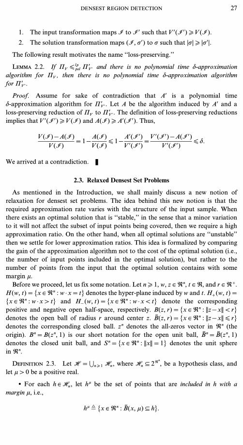
Before we proceed, let us fix some notation. Let n \ 1, w, z ¥Rn, t ¥R, and r ¥R+.H(w, t)={x ¥Rn : w ·x=t} denotes the hyper-plane induced by w and t.H+(w, t)={x ¥Rn : w ·x > t} and H−(w, t)={x ¥Rn : w ·x < t} denote the correspondingpositive and negative open half-space, respectively. B(z, r)={x ¥Rn : ||z−x|| < r}denotes the open ball of radius r around center z. B̄(z, r)={x ¥Rn : ||z−x|| [ r}denotes the corresponding closed ball. zn denotes the all-zeros vector in Rn (theorigin). Bn=B(zn, 1) is our short notation for the open unit ball, B̄n=B̄(zn, 1)denotes the closed unit ball, and Sn={x ¥Rn : ||x||=1} denotes the unit spherein Rn.

Definition 2.3. Let H=1n \ 1 Hn, where Hn ı 2Rn, be a hypothesis class, and

let m > 0 be a positive real.

• For each h ¥Hn, let hm be the set of points that are included in h with amargin m, i.e.,

hm ¸ {x ¥Rn : B̄(x, m) ı h}.


• Given a finite multiset P …Rn, let

Vm(n, P) ¸ maxh ¥Hn

|P 5 hm|.

In other words, Vm(n, P) denotes the maximum number of points in P (accountingfor their multiplicity) that can be included in a hypothesis from Hn with margin m.

• The m-relaxed densest set problem for H is defined as the Vm-relaxation of thedensest set problem for H.

We use Pm to denote the m-relaxation PVm of the problem P.

2.4. Some Known Hardness-of-Approximation Results

We shall base our hardness reductions on two known results.

Theorem 2.4 (Håstad [9]). Assuming P ]NP, for any d < 1/22, there is nopolynomial time d-approximation algorithm for MAX-E2-SAT.

Theorem 2.5 (Ben-David, Eiron, and Long [2]). Assuming P ]NP, for anyd < 3/418, there is no polynomial time d-approximation algorithm for BSH.

Claim 2.6. BSH [ lppol DOH.

Proof. By adding a coordinate one can translate hyper-planes to homogeneoushyper-planes (i.e., hyper-planes that pass through the origin). To get from thehomogeneous hyper-planes separating problem to the densest hemisphere problemone applies the standard scaling and reflection tricks.2 L

2 By scaling, we mean that each point is projected to the unit sphere. Clearly, a homogeneous hyper-plane assigns the same classification label to the point and its projection. By reflection, we mean that apoint p on the sphere that belongs to P− is replaced by its ‘‘mirror-point’’ −p which is considered as amember of P+. With this transformation, we can forget the labels and obtain an instance of the DensestHemisphere Problem. (See Chapter 5.4 of [7], for instance.)

Corollary 2.7. Assuming P ]NP, there is no polynomial time d-approx-imation algorithm for DOH, for any d < 3/418.

3. THE RELAXED DENSEST CUBE PROBLEM

We present a (rather simple) algorithm, Algorithm 3.1 below, which solves the1/4-relaxation of the DAC problem in polynomial time. We complement this resultby showing that the m-relaxation of DAC is NP-hard (and, in fact, even NP-hardto approximate) for each m < 1/4. Thus (despite its simplicity), Algorithm 3.1already solves the hardest relaxation of DAC that can be solved by any polynomialtime algorithm (unless P=NP).

An axis aligned cube with edge length u will be briefly called u-cube in whatfollows. Let W be a 1-cube. Note that the points which are contained in W withmargin 0 [ m [ 1/2 are contained in a concentric (1−2m)-sub-cube of W. (Figure 1illustrates this observation.)


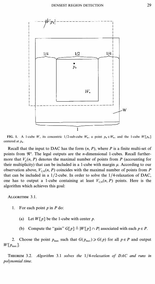
FIG. 1. A 1-cube W, its concentric 1/2-sub-cube Wg, a point pg ¥Wg, and the 1-cube W[pg]centered at pg.

Recall that the input to DAC has the form (n, P), where P is a finite multi-set ofpoints from Rn. The legal outputs are the n-dimensional 1-cubes. Recall further-more that Vm(n, P) denotes the maximal number of points from P (accounting fortheir multiplicity) that can be included in a 1-cube with margin m. According to ourobservation above, V1/4(n, P) coincides with the maximal number of points from Pthat can be included in a 1/2-cube. In order to solve the 1/4-relaxation of DAC,one has to output a 1-cube containing at least V1/4(n, P) points. Here is thealgorithm which achieves this goal:

Algorithm 3.1.

1. For each point p in P do:

(a) LetW[p] be the 1-cube with center p.

(b) Compute the ‘‘gain’’ G[p]¸ |W[p] 5 P| associated with each p ¥ P.

2. Choose the point pmax such that G(pmax) \ G(p) for all p ¥ P and outputW[pmax].

Theorem 3.2. Algorithm 3.1 solves the 1/4-relaxation of DAC and runs inpolynomial time.


FIG. 2. The point triplet associated with the 2-clause v1 K ¬ v3 in the {v1, v2, v3}-space, the cubecorresponding to the satisfying assignment (v1, v2, v3)=(0, 1, 0), and (at top of it) the cube correspond-ing to the falsifying assignment (v1, v2, v3)=(0, 1, 1).

Proof. Let Wg be the 1/2-cube which contains V1/4(n, P) points. Let pg be apoint from Wg 5 P (arbitrarily chosen). Obviously W[pg] (the 1-cube with centerpg) containsWg as subcube. (Figure 1 illustrates this observation.) Therefore,

G(pmax)=|W[pmax] 5 P| \ |W[pg] 5 P| \ |Wg 5 P|=V1/4(n, P).

It follows that Algorithm 3.1 solves the 1/4-relaxation of DAC. It clearly runs inpolynomial time. L

The next result shows that the 1/4-relaxation of DAC is the hardest relaxationwhich can be solved in polynomial time.

Theorem 3.3. For every 0 [ m < 1/4, MAX-E2- SAT [ lppol DACm.

Proof. Let 0 [ m < 1/4 be fixed. Recall that we can view 1-cubes, containing aset of points with margin m, as (1−2m)-cubes containing the same set of points. Thepoint in Rn whose ith coordinate equals 1−2m and whose other coordinates equalzero is denoted by pmi in what follows.

We will define a loss-preserving reduction from MAX-E2-SAT to the m-relax-ation of DAC. (Compare with Definition 2.1.) The following constructions areillustrated in Fig. 2.

First, we define a mapping f from input instances of MAX-E2-SAT (over nvariables) to finite multi-sets in Rn. Let v1, ..., vn be the variables that appear in thepropositional formulas, and let ¬ v1, ..., ¬ vn denote their negations, respectively.Let h be the function which maps vi to pmi and ¬ vi to −pmi . Given a 2-clause l1 K l2,define the point triplet

f(l1 K l2) ¸ {h(l1)+h(l2), −h(l1)+h(l2), h(l1)−h(l2)}.


Informally, we associate with each 2-clause c three points in the plane spanned bythe coordinates that correspond to the variables of c. These three points representthe three satisfying assignments for c.

Finally, we extend the definition of f from 2-clauses to collections of 2-clauses bysetting

f(C)¸ 0c ¥ Cf(c),

where the union of sets should be interpreted as multi-set. Obviously, f(C) can beconstructed from C in polynomial time. Note that any 1-cube can contain at mostone of the three points associated with a clause, which leads to a 1–1 correspon-dence between points contained and clauses satisfied. Details follow.

Let a=(a1, ..., an) ¥ {0, 1}n be an assignment to (v1, ..., vn) which satisfies themaximal number, say sg, of 2-clauses from C. We have to show that there exists a(1−2m)-cube which contains at least sg points of the multi-set f(C). SettingI[0]=[−(1−2m), 0] and I[1]=[0, 1−2m], the (1−2m)-cube Wa=×ni=1 I[ai]serves this purpose. More precisely,Wa contains one of the three points of f(c) iff asatisfies c. Thus,Wa contains sg points of f(C).

Let now W=×ni=1 Ii be a 1-cube which contains s points from f(C). Note thateach cube which contains at least two points of the point triplet f(c) must have sidelength at least 2(1−2m) > 1. Thus, W contains at most one point of each triplet. Itfollows that there are s ‘‘designated’’ 2-clauses in C with the property that one pointof the associated point triplet belongs to W. Setting ai=1 if interval Ii contains1−2m and ai=0 otherwise, we obtain an assignment a=(a1, ..., an) to (v1, ..., vn)which satisfies precisely the s designated 2-clauses. Clearly, a can be computed fromC and W in polynomial time. This completes the loss-preserving reduction fromMAX-E2-SAT to DACm. L

Corollary 3.4. For every 0 [ m < 1/4 and for every 0 [ d < 1/22, there is nopolynomial time d-approximation algorithm for the m-relaxation of DAC (unlessP=NP).

4. HARDNESS OF THE DENSEST BALL PROBLEM

In this section we prove a hardness-of-approximation result for the DOBproblem (Theorem 4.2 below). We refer to H+(w, 0) as an open hemisphere becausewe use the hyper-plane H(w, 0) as a separator of the unit sphere Sn into two hemi-spheres. We may assume that ||w||=1 because for all l > 0, H+(w, 0)=H+(lw, 0).

Lemma 4.1. DOH [ lppol DOB.

Proof. Let I=(n, P) be a given input to DOH, where P is a multi-set of pointsin Sn. We choose the trivial input transformation IWI, i.e., I=(n, P) is alsoconsidered as input to DOB.

Let C(w, P) be the multi-set of points from P that also belong to H+(w, 0), andlet CŒ(z, P) be the multi-set of points from P that also belong to B(z, 1). The


reduction from DOH to DOB is now accomplished by proving the followingstatements:

-w ¥ Sn, ,z ¥Rn, C(w, P) ı B(z, 1) (3)

-z ¥Rn, CŒ(z, P) ıH+(z, 0). (4)

These statements certainly imply that there is a loss-preserving reduction fromDOH to DOB. (Compare with Definition 2.1.)

To prove statement (3), we set m=minp ¥ C(w, P) |w ·p|. This implies that w·q \m > 0 for all q ¥ C(w, P). We claim that z=mw is an appropriate choice for z; i.e.,each q ¥ C(w, P) also belongs to B(z, 1). Using w·w=q·q=1, this claim is evidentfrom the following calculation:

||z−q||2=(z−q) · (z−q)

=z· z−2z · q+q·q

=m2w·w−2mw·q+q·q

=m2−2mw·q+1

[ m2−2m2+1

=1−m2

< 1.

In order to prove statement (4), we have to show that each q ¥ CŒ(z, P) satisfiesz · q > 0. To this end, note first that q ¥ CŒ(z, P) implies q · q=1 and

1 > ||z−q||2=z·z−2z · q+q·q=z· z−2z · q+1 \ −2z · q+1.

Clearly, this implies that z · q > 0. L

Applying Corollary 2.7 we readily get

Theorem 4.2. Assuming P ]NP, there is no polynomial time d-approximationalgorithm for DOB, for any d < 3/418.

As shown in [4], a similar result holds for the Densest Closed Ball problem.

Theorem 4.3 (Ben-David and Simon [4]). Assuming P ]NP, there is nopolynomial time d-approximation algorithm for DCB, for any d < 1/198.

5. COMPUTATION OF DENSE BALLS

We know from Section 4 that it is an NP-hard problem to find an (approxima-tely) densest (open or closed) ball for a given multi-set of points in Rn. In thissection, we show that, for each constant 0 < m [ 1, the m-relaxation of this problemcan be solved optimally in polynomial time. For the sake of exposition, we restrictthe following discussion to closed balls. Also, for brevity, we use r-ball to refer aball with radius r.


Let B̄ be a 1-ball. Note that the points which are contained in B̄ with margin mform the concentric (1−m)-sub-ball of B̄. It follows that an algorithm that solvesthe m-relaxation of DCB on input (n, P) must output the center of a 1-ball B̄ suchthat |B̄ 5 P| \ |B̄g 5 P| for every (1−m)-ball B̄g. A simple scaling argument showsthat instead of balls with radius 1 and 1−m, respectively, we may as well considerballs with radius 1

1−m and 1, respectively. The goal is therefore to design a family ofalgorithms which can successfully compete against the densest closed 1-ball bymeans of a closed ball of a radius slightly exceeding 1. This general idea is capturedby the following definitions.

Assume that R(k, n) is a function which maps each pair (k, n) to a positive realR(k, n) ¥R+. R is called admissible if limkQ. limnQ. R(k, n)=0.

A family (Ak)k \ 1 of polynomial time algorithms is called R-successful for DCB if,on input (n, P), Ak outputs the center of a (1+R(k, n))-ball B̄ such that|B̄ 5 P| \ |B̄g 5 P| for every 1-ball B̄g.

Lemma 5.1. If there exists a family of polynomial time algorithms which isR-successful for an admissible function R, then the m-relaxation of DCB can be solvedin polynomial time for each m > 0.

Proof. Choose k such that for all sufficiently large n, R(k, n) [ m1−m . Let (n, P)

be the input to DCB and assume that n is sufficiently large. Define scaling factor

l ¸11−m

=1+m

1−m.

Note that 1+R(k, n) [ l and 1/l=1−m. Apply the algorithm Ak (the kth memberof the R-successful family) to input (n, l ·P), where l ·P ¸ {l · p | p ¥ P}. If Akoutputs center z, then output center 1l z. Since Ak belongs to an R-successful family,B̄(z, 1+R(k, n)) does not contain fewer points from l ·P than any 1-ball. We canmake the same claim a fortiori for B̄(z, l). It follows that B̄(z/l, 1) does notcontain fewer points from P than any (1−m)-ball. L

The main result of this section is:

Theorem 5.2. For each m > 0, the m-relaxation of DCB can be solved inpolynomial time.

According to Lemma 5.1, the theorem is obtained once we have presented anR-successful family of polynomial time algorithms for an admissible function R. Tothis end, we proceed as follows. In Section 5.1, we present a generic family of algo-rithms for DCB containing some programmable parameters. The appropriatesetting of these parameters requires some geometric insights which are provided inSection 5.2. Three concrete (families of) algorithms for DCB are analyzed inSections 5.3 and 5.4: the Center-of-Gravity algorithm, the Smallest-Ball algorithm,and the Equal-Distance algorithm. The first algorithm is R1-successful forR1(k, n)=`1/k. The other two algorithms are both R2-successful for R2(k, n)=`(n−k+1)/(kn). R1 and R2 are both admissible. Furthermore, R2(k, n) [`1/kwith equality when n approaches infinity. According to Lemma 5.1, the members of


the R1- and R2-successful families solve the m-relaxations of DCB. For a given m, itsis sufficient to use an algorithm Ak such that `1/k [ m

1−m . For example, k=K1/m2Lis a possible choice.

5.1. A Generic Algorithm for the Densest Ball Problem

Let Z denote a function which maps finite multi-sets Q of points from Rn topoints in Rn. Let R denote a function which maps pairs (k, n) to positive reals.Here is the high level description of our generic algorithm for DCB:

Algorithm 5.3. Let Z, R, k be fixed. Algorithm AZ, Rk proceeds as follows oninput (n, P):

1. For each multi-set Q containing at most k points from P (possibly withrepetitions), compute two quantities associated with Q:

• the ‘‘candidate center’’ Z(Q) ¥Rn,

• the ‘‘gain’’ G(Z(Q))¸ |P 5 B̄(Z(Q), 1+R(k, n))| realized by Z(Q).

2. Choose the candidate center Zmax that realizes the maximum gain andoutput Zmax.

Before we present some concrete choices for the functions Z, R, we brieflymention the following implementation details for the generic algorithm:

Fixed Size Multisets (FSM). If the generic algorithm is run in FSM-mode,then we check only multi-sets Q of fixed size k.

No Repetitions (NR). If the generic algorithm is run in NR-mode, then weconsider sets Q instead of multi-sets.

Here are three concrete choices for the Z- and the R-function, respectively, whichwill be analyzed in the course of the next subsections:

Center-of-Gravity. The Center-of-Gravity algorithm is obtained from thegeneric algorithm AZ, Rk when we use the following functions in the roles of Z and R,respectively:

ZCG(Q)¸1|Q|· Cq ¥ Qq (5)

R1(k, n)¸`1/k. (6)

We will use the simple notation ACGk instead of AZCG, R1k .

Smallest-Ball. Let ZSB(Q) be the center of the smallest ball containing Q and

R2(k, n)¸=n−k+1kn

. (7)

The Smallest-Ball algorithm uses ZSB and R2 in the roles of Z and R, respectively.We will use the simple notation ASBk instead of AZSB, R2k .


Equal-Distance. Let ZED(Q) be the point which has the same Euclideandistance to all q ¥ Q and belongs to the same affine sub-space as Q.3 The Equal-

3 It is not hard to see that ZED(Q) is well-defined if |Q| [ n+1 and the points in Q are in generalposition.

Distance algorithm uses ZED and R2 in the roles of Z and R, respectively.4 We will

4 If the points in Q are not in general position, the algorithm may output an arbitrary candidate centerby default.

use the simple notation AEDk instead of AZED, R2k .

ACGk is run in FSM-mode. ASBk and AEDk are run in NR-mode.Here are some brief comments on the computational complexity of these algo-

rithms. Note first that it is not necessary to evaluate the square root. For instance,in order to check whether a point x is included in a ball of radius `1/k around acenter z, one checks whether the square of the Euclidean distance between x and z(which can be expressed as a scalar product) is bounded by 1/k. Note secondthat all three algorithms perform an exhaustive search through O(mk) candidate(multi-)sets. For each fixed (multi-)set, there is a polynomial time bound. ACGk is thesimplest algorithm, because each center of gravity is found in linear time. In orderto find the center of the smallest ball that contains a given set Q, one has to solve aquadratic programming problem subject to linear constraints. In order to findZED(Q), it is sufficient to solve a system of linear equations because ZED(Q) can beexpressed as the intersection of hyper-planes (after a coordinate transformationwhich maps the points in the appropriate subspace).5 Thus, ASBk requires more

5 In the plane, this is the well-known fact from Euclidean Geometry that the point with the same dis-tance to each corner of a triangle is uniquely given as the intersection of the perpendicular bisectors ofthe sides of this triangle. Clearly, each perpendicular bisector may be described by a linear equationwhose coefficients are easily obtained from the corners of the triangle. The system of linear equations forthe general case is obtained as a straightforward generalization of this classical result.

computational resources than AEDk , which, in turn, requires more computationalresources than ACGk .

All three algorithms share a common property: they are ‘‘compatible withtranslation and scaling.’’ More precisely, let

z0+P¸ {z0+p | p ¥ P} and l ·P ¸ {l · p | p ¥ P}

for each z0 ¥Rn and l > 0. We say that Z is compatible with translation if equation

Z(n, z0+P)=z0+Z(n, P)

is valid for each choice of n, P, z0. We say that Z is compatible with scaling ifequation

Z(n, l ·P)=l ·Z(n, P)

is valid for each choice of n, P, l. The following result is fairly obvious:


Lemma 5.4. The functions ZCG, ZSB, and ZED are compatible with translation andscaling.

Algorithms which are compatible with translation exhibit a nice feature. Theirperformance analysis can be restricted without loss of generality to ‘‘normalizedinputs.’’ Recall that B̄n denotes the closed unit ball with center at the origin zn (theall-zeros vector). We say that an input (n, P) for DCB is normalized if the followingholds:

• B̄n is a densest closed 1-ball on input (n, P).

• Each closed ball of radius less than 1 contains fewer points from P than B̄n.

The following result is obvious:6

6 We briefly note that compatibility with scaling, although irrelevant in our restricted setting, becomesmeaningful in a more general setting, where the output of Ak is compared with the densest ball of radiusr0 (possibly different from 1) and where r0 is given to Ak as an additional input parameter. Nowcompatibility with scaling allows us to restrict the analysis to normalized inputs with r0=1.

Lemma 5.5. Let (Ak) be a family of algorithms for DCB which is compatible withtranslation. If (Ak) is R-successful on each normalized input, then (Ak) is R-successful(on each input).

5.2. Full and Partial Spanning Sets for Smallest Balls

Let B be an open n-dimensional ball and B̄ the corresponding closed ball. Thecenter of B is denoted as zB. The boundary of B̄, called B-sphere hereafter, isdenoted as SB. Each hyperplane H partitions Rn into the three sets H+, H− (theopen half-spaces induced by H) and H itself. Each hyper-plane H which passesthrough zB cuts the B-sphere SB into two open B-hemispheres, namely SB 5H+ andSB 5H− . Let P ıRn. The following lemma presents necessary and sufficientconditions for B̄ being the smallest ball containing P.

Lemma 5.6. Assume that P is contained in B̄. The following statements areequivalent:

A1. B̄ is the smallest ball containing P.

A2. The points in P 5 SB are not contained in any open B-hemisphere.A3. The convex hull K of P 5 SB contains zB.

Proof. Let ¬ A1, ¬ A2, ¬ A3 denote the negations of the statements A1, A2,A3, respectively. We will prove the implications ¬ A3S ¬ A2, ¬ A2S ¬ A1, andA3S A1.

Let us start with the implication ¬ A3S ¬ A2. Assume that K does not containzB. Without loss of generality, K ]” (because otherwise P 5 SB=” and ¬ A2trivially holds). The following reasoning is illustrated in Fig. 3. Let p be the point inK with a minimal distance d > 0 to zB, Lp the line segment from zB to p, and Hp thehyper-plane through p that is orthogonal to Lp. The fact that K is a convexpolyhedron and the choice of p imply that Hp does not intersect the interior of K. IfH −p denotes the hyper-plane that is parallel to Hp and passes through zB (obtained


FIG. 3. A non-smallest ball containing a given set of points.

by a parallel shift of Hp along Lp), then K is totally contained in one of the openhalf-spaces induced by H −p. The points in P 5 SB are therefore contained in one ofthe open B-hemispheres induced by H −p.

We proceed with the proof for the implication ¬ A2S ¬ A1. The followingreasoning is illustrated in Fig. 3. Assume that H is a hyper-plane through zB suchthat the points in P 5 SB are contained in one of the open B-hemispheres inducedby H. Let R be the ray that starts in zB and is directed orthogonally away from Htowards the hemisphere containing P 5 SB. Let Be be the open ball obtained from Bby performing an e-shift of center zB along R. It follows that there exists an e > 0such that Be contains P. Since Be is open, it can be shrunken and still contain P. Itfollows that B̄ is not the smallest ball containing P.

We finally show the implication A3S A1. Assume that zB ¥K. The followingreasoning is illustrated in Fig. 4. Let BŒ be a ball with center zBŒ such that zBŒ ] zBand P ı B̄Œ. We have to show that the radius rŒ of BŒ is greater than the radius r ofB. Let L be the line segment from zB to zBŒ. Let H be the hyper-plane through zBwhich is orthogonal to L, H+ the open half-space containing zBŒ and H− the otheropen half-space. Since zB ¥K, H− must contain at least one point p of P 5 SB.When we move a point z along L from zB to zBŒ, its distance to p strictly increases.Since the distance between zB and p coincides with r and the distance between zBŒand p is a lower bound on rŒ, we get rŒ > r. L

Let Q ¥Rn, |Q| [ n+1, be a set of points in general position. The convex hull ofQ is then called the simplex induced by Q and denoted as S(Q). Occasionally, wewill blur the distinction between Q and the induced simplex and use the notation Qfor both objects. Recall that each polyhedron in Rn can be partitioned into


FIG. 4. A smallest ball containing a given set of points.

simplexes (which corresponds to a triangulation of a polygon in the plane). Thefollowing definition relates simplexes to balls:

Definition 5.7. Let B̄ be a ball in Rn and let Q …Rn consist of at most n+1points that are in general position. Q is called a spanning set for B̄ if Q … SB andzB ¥S(Q). A spanning set for an n-dimensional ball is called degenerated if itcontains at most n points.

The following results are (more or less) immediate consequences of Lemma 5.6.

Corollary 5.8. If Q is a spanning set for B̄, then ZSB(Q)=ZED(Q)=zB.

Figure 5 illustrates Corollary 5.8.

Corollary 5.9. Let B̄ be the smallest n-dimensional ball containing a finite set Pof points from Rn. Then P 5 SB contains a spanning set Q for B̄.

Proof. According to Lemma 5.6, the convex hull K of P 5 SB contains zB. Forma simplicial decomposition of the polyhedron K. One of the simplexes in thisdecomposition, say S, must contain zB. It follows that the vertex set Q of S is aspanning set for B̄. L

Let us briefly explain how we will use the concept of spanning sets. Recall thatwe can restrict ourselves to a normalized input (n, P), among whose smallestdensest balls is the unit ball B̄n with center zn (the all-zeros vector). According toCorollary 5.9, P 5 Sn contains a spanning set Qn for B̄n. Recall that |Qn| [ n+1. Wewant to argue that the generic algorithm AZ, Rk computes at least one candidatecenter Z(Q) that is close to the origin zn. Note that ZSB(Qn)=ZED(Qn)=zn. Thus,the Smallest-Ball and the Equal-Distance algorithms would both find the optimalcenter if they inspected the full spanning set Qn. However, the generic algorithm


FIG. 5. (a) A 2-dimensional example: a spanning set Q of size 3 for a 2-dimensional ball B̄. (b) A3-dimensional example: a degenerated spanning set Q of size 3 for a 3-dimensional ball B̄. in both cases,zB=ZSB(Q)=ZED(Q).

inspects only (multi-)sets Q of size at most k, and k is much smaller than n ingeneral. The hope is that Qn contains a small subset Q such that Z(Q) comesalready close to the origin. This motivates the following definition.

Definition 5.10. Let R be a function which maps a pair (k, n) to a positive realR(k, n) ¥R+. We say that function Z is an R-approximator if the following holds:

• Z is compatible with translation and scaling.

• For each k \ 1, for each normalized input (n, P), and for each spanning setQn for B̄n, there exists a multi-set7 Q ı Qn of size at most8 k such that

7 Replace ‘‘multi-set’’ by ‘‘set’’ if the generic algorithm is run in NR-mode.8 Replace ‘‘at most’’ by ‘‘exactly’’ if the generic algorithm is run in FSM-mode.

||Z(Q)−zn||=||Z(Q)|| [ R(k, n).

The following result is fairly obvious from the above discussions:

Lemma 5.11. If Z is an RŒ-approximator and RŒ(k, n) [ R(k, n) for each pair(k, n), then (AZ, Rk ) as R-successful.

Let us briefly summarize what we have achieved so far. Setting RŒ=R, Lemma5.11 implies that a Z-function which is an R-approximator leads to an instantiation(AZ, Rk ) of the generic algorithm that is R-successful. Lemma 5.1 states that anR-successful family of algorithms (for an admissible function R) can be used tosolve the m-relaxation of DCB in polynomial time (for each m > 0). In order toprove the main result of this section, Theorem 5.2, it is sufficient to analyze thefunctions ZCG, ZSB, ZED and to prove that each of them is an R-approximator forsome admissible function R. This is exactly what we will do in the course of thenext two subsections.


5.3. The Center-of-Gravity Algorithm

The analysis of the Center-of-Gravity algorithm builds on Theorem 5.12, which isattributed to Maurey [8]. A proof for this is theorem can be found in [1, 5, 12].

Theorem 5.12 (Maurey [1]). Let F be a vector space with a scalar product( · , · ) and let ||f|| ¸`(f, f) be the induced norm on F. Suppose G ı F and that, forsome c > 0, ||g|| [ c for all g ¥ G. Then for all f from the convex hull of G and allk \ 1 the following holds:

infg1, ..., gk ¥ G

>1kCk

i=1gi−f> [=

c2−||f||2

k.

The proof makes use of the probabilistic method. It is essential for the validity ofthe theorem that the elements g1, ..., gk taken from G in the inf-expression are notnecessarily distinct from each other.

Corollary 5.13. ZCG is a`1/k- approximator.

Proof. We apply Theorem 5.12 to the following special situation:

• F=Rn with the standard scalar product. The induced norm is the Euclideannorm.

• G=Qn, where Qn is a spanning set for the unit ball B̄n. Recall that|Qn| [ n+1 and all points of Qn reside on the unit sphere Sn. Moreover, the convexhull of Qn is the simplex induced by Qn, which contains the center zn of B̄n (theorigin).

• Choose f=zn (the origin). It follows that ||f||=0. Since G=Qn … Sn, thebound c in Theorem 5.12 can be safely set to 1 in our particular application. Thusthe upper bound given in the theorem simplifies to`1/k.

It follows from this discussion that there exist points g1, ..., gk taken from Qn (pos-sibly with repetitions) such that their center of gravity has distance at most `1/kfrom the origin. Thus, ZCG is a`1/k-approximator. L

5.4. The Smallest-Ball and the Equal-Distance Algorithm

Throughout this subsection, Qn denotes a spanning set for the closed unit ball B̄n.Recall that Qn consists of (at most n+1) points in general position that reside onthe unit sphere Sn. The simplex S(Qn) induced by Qn contains the origin zn. Byabuse of notation, we will identify Qn with S(Qn).

Each subset Q of Qn of size k induces the sub-simplex of Qn with vertex set Q,briefly called a k-sub-simplex hereafter. Again, we identify Q with the induced k-sub-simplex. An n-sub-simplex is called a face, a 2-sub-simplex is called an edge, and a1-sub-simplex is called a vertex of the simplex Qn.

Let Q be a face of Qn and HQ its supporting hyper-plane. Note that the intersec-tion of HQ and B̄n is a closed (n−1)-dimensional ball, say B̄Q. Its center and its


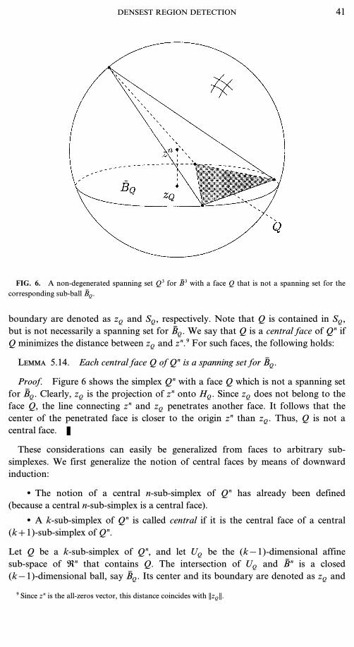
FIG. 6. A non-degenerated spanning set Q3 for B̄3 with a face Q that is not a spanning set for thecorresponding sub-ball B̄Q.

boundary are denoted as zQ and SQ, respectively. Note that Q is contained in SQ,but is not necessarily a spanning set for B̄Q. We say that Q is a central face of Qn ifQ minimizes the distance between zQ and zn.9 For such faces, the following holds:

9 Since zn is the all-zeros vector, this distance coincides with ||zQ ||.

Lemma 5.14. Each central face Q of Qn is a spanning set for B̄Q.

Proof. Figure 6 shows the simplex Qn with a face Q which is not a spanning setfor B̄Q. Clearly, zQ is the projection of zn onto HQ. Since zQ does not belong to theface Q, the line connecting zn and zQ penetrates another face. It follows that thecenter of the penetrated face is closer to the origin zn than zQ. Thus, Q is not acentral face. L

These considerations can easily be generalized from faces to arbitrary sub-simplexes. We first generalize the notion of central faces by means of downwardinduction:

• The notion of a central n-sub-simplex of Qn has already been defined(because a central n-sub-simplex is a central face).

• A k-sub-simplex of Qn is called central if it is the central face of a central(k+1)-sub-simplex of Qn.

Let Q be a k-sub-simplex of Qn, and let UQ be the (k−1)-dimensional affinesub-space of Rn that contains Q. The intersection of UQ and B̄n is a closed(k−1)-dimensional ball, say B̄Q. Its center and its boundary are denoted as zQ and


SQ, respectively. Q is contained in SQ, but is not necessarily a spanning set for B̄Q.The following result easily follows by induction:

Lemma 5.15. Each central k-sub-simplex Q of Qn is a spanning set for B̄Q.

Note furthermore that there exists at least one central k- sub-simplex Q of Qn forall k=0, ..., n.

Assume that Q is a k-sub-simplex of Qn which is a spanning set for B̄Q. FromCorollary 5.8, we know that ZSB(Q)=ZED(Q)=zQ. According to Lemma 5.15, thisequality holds in particular for each central k-sub-simplex. The analysis of theSmallest-Ball and the Equal-Distance algorithm is based on the following

Lemma 5.16. Let Q be a central k-sub-simplex of Qn. Then ||zQ || [ R2(k, n),where R2(k, n) is the function given by Eq. (7).

Lemma 5.16, whose (somewhat lengthy) proof is given in the appendix, basicallyconcludes the analysis of the Smallest-Ball and the Equal-Distance algorithm:

Corollary 5.17. ZSB and ZED are both R2-approximators.

Proof. Let Qn be a spanning set for B̄n. Let Q be a central k-sub-simplex of Qn.According to Lemma 5.15, Q is a spanning set for B̄Q. It follows thatZSB(Q)=ZED(Q)=zQ. According to Lemma 5.16, ||zQ || [ R2(k, n). L

6. CONCLUSIONS

We briefly mention some possible extensions of our work and some openquestions:

• All hardness results presented in this paper remain true when we disallowmulti-sets and consider only points of ‘‘multiplicity’’ 1. The proofs would becometechnically more involved10 (without providing much more insight).

10 Basically, an input point with multiplicity j must be replaced by j pairwise distinct points withapproximately the same location in Rn.

• The notion of m-relaxation can be generalized (in the obvious fashion) from aconstant m to a function m in parameters n (the dimension) or m (the number ofpoints in the input instance).

• It can be shown [4] that the `1/(45n)-relaxation of DOH and the1/(90n)-relaxation of DOB (or DCB) are NP-hard (and, in fact, even NP-hard toapproximate). On the other hand, we have shown in this paper that the m-relaxationof these problems can be solved in polynomial time for each constant m > 0. Theseresults leave open the computational complexity of the m-relaxation of DOH (orDOB, DCB, respectively), when m=m(n) approaches zero asymptotically slowerthan`1/n (or 1/n, respectively).

• The NP-hardness of the 1/(90n)-relaxation of DCB shows that we cannotexpect an R-successful algorithm for DCB—for an admissible function R=R(k, n)—with a polynomial time bound in k. However, the time boundO(mk) poly(n, m) achieved by our algorithms ACG, ASB, AED might be improved to


time bounds of the form f(k) poly(n, m) for some function f. In the parameterizedcomplexity framework [6], this is the question of whether the (1/k)-relaxation ofDCB is fixed-parameter tractable.

• In this paper, we investigated the problem of maximizing the empiricaldensity (as opposed to the true density with respect to an input generating distribu-tion). From this purely combinatorial perspective, the Center-of-Gravity algorithmis almost as successful as the (computationally more expensive) Equal-Distancealgorithm (not to speak of the even more expensive Smallest-Ball algorithm). Weexpect however AED and ASB to exhibit a superior statistical generalization. Thevalidity of this claim will be the subject of future research.

APPENDIX A: PROOF OF LEMMA 5.16

Recall that Qn denotes a spanning set for the unit ball B̄n. Let Q be a centralk-sub-simplex of Qn. Recall that the intersection of B̄n with the lowest dimensionalaffine sub-space of Rn that contains Q yields a (k−1)-dimensional ball BQ withcenter zQ. We have to show that ||zQ || [ R2(k, n), where R2 is the function given byEq. (7).

If Qn is a degenerated spanning set for B̄n, then it is a non-degenerated spanningset for a lower-dimensional unit ball, say for B̄nŒ such that nŒ < n. Since R2(k, nŒ) <R2(k, n) if nŒ < n, we may restrict ourselves to the non-degenerated case in whatfollows. Thus, Qn consists of n+1 vertices, say q0, ..., qn, that are in general positionand reside on the unit sphere Sn. Viewed as simplex, Qn contains the origin.

We apply induction on n+1−k. The case k=n+1 (induction base) is trivial.The only (n+1)-sub-simplex of Qn is Qn itself. Thus zQ coincides with the origin zn.Therefore, ||zQ ||=||zn||=0=R2(k, n+1). The following result covers the case k=n.

Lemma A.1. Let Q be a central face of Qn. Then ||zQ || [ 1/n.

Proof. We will derive several formulas for the (n-dimensional) volume V of thesimplex Qn (in terms of ||zQ || and some other parameters) which algebraically implythat ||zQ || [ 1/n.

Let Qi=Qn0{qi}. Recall that, by abuse of notation, Qi denotes also the faceinduced by the vertices of Qn0{qi}. Let Vi denote the ((n−1)-dimensional) volumeof Qi. Let Q −i be the simplex that is obtained from Qn when we replace vertex qi bythe origin, and let V −

i denote the (n-dimensional) volume of Q −i. Let finally hidenote the distance between vertex qi and face Qi (i.e., the height of Qn whenviewed as simplex on top of face Qi), and let ri denote the distance between theorigin and Qi (i.e., the height of Q −i when viewed as simplex on top of face Qi). Anillustration of these notations may be found in Fig. 7. Note that

||zQ ||= mini=0, ..., n

ri (8)

because Q is a central face.


FIG. 7. A non-degenerated spanning set Q3 and the decomposition of the corresponding simplexinto sub-simplexes. The serpentine lines indicate segments of length 1.

We proceed with the following auxiliary result:

Claim A.2. For all i=0, ..., n, hi [ 1+ri.

Proof of the Claim. Let zi be the projection of the origin to face Qi. Clearly, hi isnot greater than the distance from qi to zi, i.e., hi [ ||zi−qi ||. As a vertex of Qn, qihas distance 1 from the origin, and (by definition of ri) the origin has distance ri tozi. Using the triangle inequality, we conclude that hi [ ||zi−qi || [ 1+ri. L

We are now prepared to derive various formulas for V. Recall that then-dimensional volume of a simplex in Rn, viewed as simplex of height hg on top of aface Qg with (n−1)-dimensional volume Vg, is given by hgVg/n. In combinationwith Claim A.2, we get

V=hiVin

[(1+ri)Vin

. (9)

Summing over all i, we obtain

(n+1)V=1n(h0V0+·· ·+hnVn) [

1n((1+r0)V0+·· ·+(1+rn)Vn). (10)

Since Qn partitions into Q −0, ..., Q−

n (up to an overlap of n-dimensional volumezero), we may alternatively write V as

V=V −

0+·· ·+V −

n=1n(r0V0+·· ·+rnVn). (11)


FIG. 8. (a) A regular simplex with 3 vertices. (b) A regular simplex with 4 vertices.

Subtracting (11) from (10), we get

nV [1n(V0+·· ·+Vn)=

O

n, (12)

where O=V0+·· ·+Vn is the ((n−1)-dimensional) volume of the surface of Qn.Dividing (11) by (12), we obtain

1n\V0O· r0+·· ·+

VnO· rn. (13)

Note that the right hand of this inequality is a convex combination of r0, ..., rn andtherefore lower-bounded by mini=0, ..., n ri=||zQ ||. This completes the proof ofLemma A.1. L

As a marginal note, we would like to mention that (12) implies that V/O [ 1/n2.Quantity 1/n2 is precisely the volume-surface ratio of the regular simplex11 with

11 A simplex is called regular if all of its edges have the same length. By symmetry, the vertices of eachregular simplex reside on the boundary of a ball around their center of gravity. The regular simplex isunique up to translation, rotation, and scaling.

n+1 vertices residing on the unit sphere Sn. (Figure 8 shows the regular simplexesin R2 and R3, respectively.) We have therefore accidentally proven that regularsimplexes (with vertices residing on the unit sphere) achieve the highest volume-surface ratio (among all simplexes whose vertices reside on the unit sphere).

We are now prepared to perform the inductive step. Let Q=Qk−1 be a centralk-sub-simplex of Qn for some k < n. It follows that there is a chain

Qk−1 … · · · … Qn−1 … Qn,

such that Q j is a (j+1)-sub-simplex of Qn for j=k−1, ..., n, and Q j is a centralface of Q j+1 for j=k−1, ..., n−1. We denote the sub-ball of B̄n, obtained by


FIG. 9. Two triangles (with a right angle at zn−1, respectively) induced by the center zn of ann-dimensional simplex Qn and the centers of some sub-simplexes of Qn. Serpentine lines indicatesegments of length 1.

intersecting B̄n with the lowest-dimensional affine sub-space containing Q j, asB̄(zj, rj). Here, zj is the center of this sub-ball and rj is the radius. Note that zncoincides with zn (the origin) and rn=1. Since zn−1=zQn−1 and Qn−1 is a central faceof Qn, Lemma A.1 yields

||zn−zn−1 ||=||zn−1 || [ 1/n. (14)

Furthermore, zk−1=zQ. We define R(k, j) ¸ ||zj−zk−1 || for j=k−1, ..., n. Notethat R(k, k−1)=0 and R(k, n)=||zk−1 ||=||zQ ||. It suffices therefore to show thatR(k, n) [ R2(k, n).

We may apply the induction hypothesis to Q as k-sub-simplex of Qn−1, keeping inmind that B̄(zn−1, rn−1) has radius rn−1 (and not radius 1). Taking the scaling factorrn−1 into consideration, the inductive hypothesis reads as

R(k, n−1) [ rn−1 ·R2(k, n−1). (15)

Let z0 be a vertex in Q. The rest of the proof, which is illustrated in Fig. 9, makesuse of the fact that the triangles induced by z0, zn−1, zn and zk−1, zn−1, zn, respec-tively, have both a right angle at zn−1. The Pythagorean Law, applied to bothtriangles, yields

r2n−1=1−||zn−1 ||2 (16)

R2(k, n)=R2(k, n−1)+||zn−1 ||2. (17)

In combination with Eqs. (15) and (14), we get

R2(k, n) [ r2n−1R22(k, n−1)+||zn−1 ||

2

=(1−||zn−1 ||2) R22(k, n−1)+||zn−1 ||

2

[ 11− 1n22 R22(k, n−1)+

1n2

=R22(k, n).


The last inequality holds because (1− ||zn−1 ||2) R22(k, n−1)+||zn−1 ||

2 is a convexcombination of R22(k, n−1) and 1 and R22(k, n−1) [ 1. This convex combination ismaximized when ||zn−1 ||2 equals its upper bound 1/n2. The last equality (expressingR2(k, n) in terms of R2(k, n−1)) is obtained by a straightforward calculation thatuses Eq. (7). It follows from our calculations that R(k, n) [ R2(k, n), whichconcludes the proof.

Finally, we would like to mention that the upper bound on ||zQ || given in Lemma5.16 is tight: if Q is a k-sub-simplex of the regular simplex with n+1 verticesresiding on Sn, then ||zQ ||=R2(k, n). We omit the straightforward inductive proofof this claim.

ACKNOWLEDGMENTS

The authors gratefully acknowledge the support of the German-Israeli Foundation for ScientificResearch and Development Grant I-403-001.06/95. This work has been supported in part also by theESPRIT Working Group in Neural and Computational Learning II, NeuroCOLT2, 27150. Thanks toRobert C. Williamson for pointing our attention to the Theorem of Maurey. Thanks to Dietrich Braessand Rüdiger Verfürth for helpful discussions concerning the proof of Lemma 5.16. Thanks to twoanonymous referees for their valuable suggestions.

REFERENCES

1. M. Anthony and P. L. Bartlett, ‘‘Neural Network Learning: Theoretical Foundations,’’ CambridgeUniv. Press, Cambridge, UK, 1999.

2. S. Ben-David, N. Eiron, and P. Long, On the difficulty of approximately maximizing agreements, in‘‘Proceedings of the 13th Annual Conference on Computational of Learning Theory, 2000,’’pp. 266–274.

3. S. Ben-David and M. Lindenbaum, Learning distributions by their density levels—A paradigm forlearning without a teacher, J. Comput. System. Sci. 55 (1997), 171–182.

4. S. Ben-David and H. U. Simon, Efficient learning of linear perceptrons, in ‘‘Advances in NeuralInformation Processing Systems 13, 2000,’’ pp. 189–195.

5. B. Carl, On a characterization of operators from lq into a Banach space of type p with someapplications to eigenvalue problems, J. Funct. Anal. 48 (1982), 394–407.

6. R. G. Downey and M. R. Fellows, ‘‘Parameterized Complexity,’’ Springer-Verlag, New York/Berlin, 1998.

7. R. G. R. O. Duda and P. E. Hart, ‘‘Pattern Classification and Scene Analysis,’’ Wiley, New York,1973.

8. R. M. Dudley, Universal Donsker classes and metric entropy, Ann. Probab. 15 (1987), 1306–1326.

9. J. Håstad, Some optimal inapproximability results, in ‘‘Proceedings of the 29th Annual Symposiumon Theory of Computing, 1997,’’ pp. 1–10.

10. D. S. Johnson and F. P. Preparata, The densest hemisphere problem, Theoret. Comput. Sci. 6 (1978),93–107.

11. N. Megiddo, On the complexity of polyhedral separability, Discrete Comput. Geom. 3 (1988),325–337.

12. G. Pisier, Remarques sur un résultat non publié de B. Maurey, in ‘‘Séminaire d’Analyse Fonc-tionelle, 1980–1981,’’ École Polytechnique, Centre de Mathématiques, Palaiseau, V.1–V.12, 1981.


the computational complexity of densest region detection

Documents