the computation of winding eddy losses in power...
TRANSCRIPT

The Computation of Winding Eddy Losses in Power
Transformers Using Analytical and Numerical Methods
Mluleki Cyril Hlatshwayo
A dissertation submitted to the Faculty of Engineering and the Built Environment, University of
the Witwatersrand, in fulfilment of the requirements for the degree of Master of Science in
Engineering.
Johannesburg, 2013

ii
Declaration
I declare that this dissertation is my own unaided work except where otherwise acknowledged. It
is being submitted for the degree of Master of Science in Engineering in the University of the
Witwatersrand, Johannesburg. It has not been submitted before for any degree or examination in
any other university.
Signed this…… day of …..………..2013
…………………………………
Mluleki Cyril Hlatshwayo

iii
Abstract
This dissertation presents the implementation of analytical and numeral methods in computing
the winding eddy losses of power transformers. It is appreciated that the computation of any
component of stray losses of a transformer is intricate and involves a multitude of variables. The
eddy current losses of a single conductor are treated using the rectangular and cylindrical
coordinates of the differential form of Maxwell’s equations. The governing equations have
limited use when the conductor thickness is increased; this is observed when thicknesses exceed
5mm. The analytical method, known as Rabins’ method is implemented in Mathematica to
evaluate local flux density quantities. The analytical method is compared to the two-dimensional
finite element method (FEM) approach. The FEM methodology is found to be robust, flexible
and fast to compute flux density components. The leakage flux distribution around the
circumference of concentric windings is studied. The windings of a three-phase, three limb
transformer that are subject to the non-homogenous distribution of the field due to the presence
of the core yokes and adjacent winding influence are modelled. The developed three-dimensional
model shows that this effect can introduce an error in the region of 32% to the radial leakage
field component. The results of the computational methods are compared to the experimental
results of the measured stray losses. The test data of the same design that has been produced
eleven times are presented. The stray losses in metal parts are evaluated and subtracted from the
net measured stray losses to give measured winding eddy losses. A large error is observed
between the calculated and measured winding eddy losses. It is further commented that the
benefits of rigorous methods in computing any stray loss component can be suppressed by the
variance of measured results of the same transformer design.

iv
Acknowledgements
I wish to thank Professor Ivan Hofsajer for his insightful and illuminating discussions, without
his patience, stimulating criticism, assistance and encouragement this work would not have been
completed. My colleagues (Matshediso Phoshoko and Mercy Tshivhilinge) who assisted with the
review of the dissertation chapters from the very beginning deserve a special mention.
I want to thank my partner Nonhle Wanda for her unconditional support. She remained patient
with me, and at times assisted with the review of the text.
I would like to sincerely thank my father, sisters and brothers for their support and
encouragement. I am indebted to my two adorable nieces Nosipho and Nokwanda Hlatshwayo
whom I draw lots of inspiration from. The help of friends and colleagues who directly or
indirectly supported me is also recognised.
Lastly, this work is supported in part by Powertech Transformers who provided resources and
funding, it is gratefully acknowledged.

v
Contents
Declaration ............................................................................................................................................ii
Abstract ............................................................................................................................................... iii
Acknowledgements ............................................................................................................................. iv
Contents ................................................................................................................................................. v
List of Figures ...................................................................................................................................... ix
List of Tables ..................................................................................................................................... xii
List of Symbols ................................................................................................................................. xiii
Introduction ........................................................................................................................................... 1
1.1. Power transformer load losses .............................................................................................. 1
1.2. Problem definition ................................................................................................................. 3
1.3. Transformer design approach ............................................................................................... 4
1.4. Research objectives ............................................................................................................... 7
1.5. Dissertation structure............................................................................................................. 8
Eddy current losses in transformers................................................................................................... 10
2.1 Winding eddy losses............................................................................................................ 12
2.2 Circulating current losses .................................................................................................... 14
2.3 Stray losses in structural parts ............................................................................................ 15
2.3.1 Tank wall losses ........................................................................................................... 16
2.3.2 Core clamp losses ........................................................................................................ 17
2.3.3 Flitch plate and outer core packet losses .................................................................... 17
2.4. Conclusion ........................................................................................................................... 18
Theory development: Analysis of eddy currents .............................................................................. 20
3.1. Electromagnetic formulation in time varying field ........................................................... 21
3.2. Analytical solution of the diffusion equation .................................................................... 24

vi
3.3. Power loss density ............................................................................................................... 28
3.4. One dimensional solution application ................................................................................ 29
3.5. Laplacian operations ........................................................................................................... 36
3.6. Eddy current solution in cylindrical coordinates ............................................................... 37
3.7. Conclusion ........................................................................................................................... 46
Evaluation of Rabins’ analytical method .......................................................................................... 47
4.1. Analytical computation of the field .................................................................................... 49
4.2. Rabins’ algorithm implementation ..................................................................................... 62
4.2.1. Assessment of the number of digits of precision ....................................................... 62
4.2.2. Number of series terms ................................................................................................ 65
4.3. Numerical approach ............................................................................................................ 68
4.4. Results discussion ................................................................................................................ 69
4.5. Conclusion ........................................................................................................................... 75
Core window effect on the calculation of winding eddy losses ...................................................... 77
5.1. Global flux density distribution .......................................................................................... 79
5.2. Core window concept .......................................................................................................... 80
5.3. Calculation of winding eddy losses .................................................................................... 82
5.4. Transformer modelling using 3-D FEM ............................................................................ 83
5.5. Results post-processing procedure ..................................................................................... 85
5.6. Circumferential field distribution ....................................................................................... 87
5.7. Effect of the winding to core yoke distance ...................................................................... 90
5.8. Transient analysis ................................................................................................................ 95
5.9. Result discussion ............................................................................................................... 101
5.10. Conclusion ..................................................................................................................... 103
Experimental results and discussion ................................................................................................ 104

vii
6.1. Load loss measurement ..................................................................................................... 105
6.1.1. Measuring circuitry .................................................................................................... 106
6.1.2. Load loss test results .................................................................................................. 107
6.2. The results of the finite element method model .............................................................. 108
6.3.1. The tank losses ........................................................................................................... 109
6.3.2. Core clamp and flitch plate losses ............................................................................ 111
6.3. Measured winding eddy losses ..................................................................................... 115
6.4. Conclusion ......................................................................................................................... 116
Conclusions and recommendations ................................................................................................. 118
7.1. Conclusion ......................................................................................................................... 118
a. Eddy currents ..................................................................................................................... 118
b. Evaluation of leakage fields .............................................................................................. 119
c. Core window effect ........................................................................................................... 119
d. Practical result ................................................................................................................... 119
7.2. Recommendations ............................................................................................................. 120
References ......................................................................................................................................... 121
Appendix A ....................................................................................................................................... 127
Single conductor analysis ................................................................................................................. 127
Simulation model .......................................................................................................................... 127
Single conductor model mesh ...................................................................................................... 128
Boundary condition assignment ................................................................................................... 128
Results: Field distribution ............................................................................................................ 129
Results: Current distribution ........................................................................................................ 130
Appendix B ....................................................................................................................................... 130
Transformer geometry of the 105MVA transformer .................................................................. 130

viii
Appendix C ....................................................................................................................................... 133
Geometry Modelling Data of the 40 MVA, 132/11kV transformer .......................................... 133
Winding design data of the 40MVA, 132/11kV transformer .................................................... 134
Example: Maxwell field calculator .............................................................................................. 134
Appendix D ....................................................................................................................................... 135
Load loss test reports .................................................................................................................... 135

ix
List of Figures
Figure Page
Figure 1.1: The breakdown of load losses into sub-components....................................................... 2
Figure 1.2: Three-dimensional geometry model showing conductive transformer components .... 5
Figure 1.3: Design of a helical winding .............................................................................................. 6
Figure 1.4: Design of a disc winding................................................................................................... 6
Figure 1.5: Loop Layer winding design .............................................................................................. 7
Figure 2.1: 2-D Cross sectional geometry of the transformer.......................................................... 11
Figure 3.1: Transformer winding coil ............................................................................................... 24
Figure 3.2: Field penetrating a conductor ......................................................................................... 25
Figure 3.3: The real and imaginary components of Hz .................................................................... 27
Figure 3.4: Real and imaginary components of the current density inside a conductor ................ 30
Figure 3.5: Edge wound strand .......................................................................................................... 31
Figure 3.6: Flat wound strand ............................................................................................................ 32
Figure 3.7: Trigonometric function ratio of Equation 3.42 versus conductor size ......................... 33
Figure 3.8: Mid flux density quantities for different conductor thicknesses .................................. 36
Figure 3.9: Cylindrical setup of the conductor, placed in the magnetic field ................................. 38
Figure 3.10: Top view of the cylindrical layout of the winding ...................................................... 39
Figure 3.11: Current density distribution within a 2mm conductor ................................................ 42
Figure 3.12: Current density distribution within a 5mm small conductor ...................................... 42
Figure 3.13: Current density distribution within large conductors (23mm) ................................... 43
Figure 3.14: Current density distribution within large conductors (50mm) ................................... 43
Figure 3.15: Integration of Modified Bessel functions at 500 mm radius ...................................... 44
Figure 3.16: Integration of Modified Bessel functions at 200 mm radius ...................................... 45
Figure 4.1: Power transformer 2-D cross sectional view ................................................................. 49
Figure 4.2: Rabins’ method solution procedure................................................................................ 50
Figure 4.3: Transformer core and winding arrangement.................................................................. 53
Figure 4.4: Distribution of current density along the window section ............................................ 54
Figure 4.5: Integration of the Modified Bessel function to evaluate Cn ......................................... 59
Figure 4.6: Integration of the Modified Bessel function to evaluate Dn......................................... 59

x
Figure 4.7: Integration of the Modified Bessel function to evaluate En ......................................... 60
Figure 4.8: Integration of Modified Bessel functions to evaluate Fn .............................................. 60
Figure 4.9: Radial flux density distribution of precision digits ranging from 10 to 20.................. 63
Figure 4.10: Radial flux density distribution of digits ranging from 30 to 50 ................................ 63
Figure 4.11: Axial flux density distribution of digits ranging from 10 to 20 ................................. 64
Figure 4.12: Axial flux density distribution for precision digits ranging from 30 to 50 ................ 64
Figure 4. 13: Radial flux density distribution when the number of terms varies from 10 to 40.... 66
Figure 4.14: Radial flux density distribution when the number of terms varies from 50 to 70..... 66
Figure 4.15: Axial flux density distribution when the number of terms varies from 10 to 40 ...... 67
Figure 4.16: Axial flux density distribution when the number of terms varies from 50 to 70 ...... 67
Figure 4.17: Maxwell simplified geometry model ........................................................................... 68
Figure 4.18: Radial flux density from FEM and Rabins’ method ................................................... 70
Figure 4.19: Axial flux density from FEM and Rabins’ method ..................................................... 71
Figure 4.20: Radial flux density distribution of Case 2 ................................................................... 72
Figure 4.21: Axial flux density distribution of Case 2 ..................................................................... 73
Figure 4.22: Radial flux density distribution of Case 5 ................................................................... 73
Figure 4.23: Axial flux density distribution of Case 5 ..................................................................... 74
Figure 4.24: Assessment of the off-set for axial flux density distribution ...................................... 75
Figure 5.1: 3-D Flux distribution during operation .......................................................................... 79
Figure 5.2: 3-phase winding transformer showing the circumference effect. ................................ 80
Figure 5.3: Winding sections situated inside the core window ....................................................... 81
Figure 5.4: Outside core window winding sections ......................................................................... 81
Figure 5.5 a: Single-phase configuration Figure 5.5 b: Three-phase configuration ............ 84
Figure 5.6 : Energy error changes per adaptive pass ........................................................................ 85
Figure 5.7: Non-model object line drawn for the acquisition of the flux density .......................... 86
Figure 5.8: Radial flux density distribution around the circumference ........................................... 88
Figure 5.9: Axial flux distribution for phase A, B and C along the circumference ....................... 89
Figure 5.10: Radial flux distribution across the winding circumference ........................................ 91
Figure 5.11: Axial flux distribution across the winding circumference .......................................... 92
Figure 5.12: Radial flux density plotted with the average value ..................................................... 93
Figure 5.13: Radial flux density plotted with the average value ..................................................... 94

xi
Figure 5.14: Sinusoidal excitation with discrete transient simulation points ................................. 95
Figure 5.15a: Radial flux density at t=0 Figure 5.15 b: Axial flux density at t=0 ...................... 96
Figure 5.16a: Radial flux density at t=0.004 Figure 5.16 b: Axial flux density at t=0.004 ..... 96
Figure 5.17a: Radial flux density at t=0.012 Figure 5.17b: Axial flux density at t=0.012 ......... 97
Figure 5.18: Flux density distribution of phase A at t =0.012 s ...................................................... 98
Figure 5.19: Flux density distribution of phase B at t =0.012 s ....................................................... 99
Figure 5.20: Flux density distribution of phase C at t =0.012 s ..................................................... 100
Figure 6.1: Three-phase load loss measuring circuitry .................................................................. 106
Figure 6.2: The leakage field on the tank walls .............................................................................. 109
Figure 6.3: Loss distribution on the surface of the tank base plate ............................................... 110
Figure 6.4: Loss distribution on the surface of the tank base plate ............................................... 110
Figure 6.5: Core clamp convergence analysis ................................................................................ 112
Figure 6.6: Loss density pattern in the core clamps and flitch plates............................................ 113

xii
List of Tables
Table Page
Table 3.1: Supplier’s maxima and minima conductor dimensions ................................................. 32
Table 4.1: Winding height cases ........................................................................................................ 71
Table 5.1: 40 MVA excitation data ................................................................................................... 84
Table 5.2: Single phase parametric design points ............................................................................ 90
Table 5.3: Calculated winding eddy loss results............................................................................. 101
Table 5.4: Single phase at the limb height of 1808 mm ................................................................. 102
Table 6.1: Measured stray losses of the tested units....................................................................... 107
Table 6.2: Tank wall, cover and base losses ................................................................................... 111
Table 6.3: Core clamp simulation results ........................................................................................ 114
Table 6.4: Flitch plate losses ............................................................................................................ 114
Table 6.5: Calculated versus measured winding eddy losses ........................................................ 115

xiii
List of Symbols
Homogenous solution first constant
Magnetic vector potential W/m
Homogenous solution second constant
Flux density vector T
B Flux density T
Br Radial flux density T
Bz Axial flux density T
BY Bottom yoke
Modified Bessel function solution constant
Modified Bessel function solution constant
Electric field vector V/m
Tangential electric field of the surface V/m
h Height of the strand mm
Magnetic field A/m
Tangential magnetic field of the surface A/m
I Region between the core and the first winding
II Region within the first winding section
III The region after the first winding onwards
Modified Bessel Function of the first kind of order zero
Modified Bessel Function of the first kind of order one
xiv
Current density vector A/m²
Current densities as Fourier series coefficients A/m²
Peak complex current density W/m2
Modified Bessel Function of the second kind of order zero
Modified Bessel Function of the second kind of order one
L Core window height
Load loss cost R/kW
na, nr Local number of axial and radial strands respectively
neT, nrT Total number of axial and radial strands respectively
No-load loss cost R/kW
Losses W
Surface loss density W/m2
Eddy current losses kW
Load losses kW
Transformer DC losses kW
Transformer stray losses kW
Transformer winding stray losses kW
Transformer winding eddy losses kW
Stray losses in metal parts W
Pea Axial component of winding eddy losses W
Per Radial component of winding eddy losses W

xv
No-load losses kW
Radial position of the core, winding (radius) mm
Price of all transformer accessories R
Works quoted net R
t Strand thickness mm
TY Top Yoke
Transformer total price R
Scalar potential
WH Winding Height mm
Arbitrary axial position of the winding section
Linear surface impedance Ω
Conductivity of the material S/m
Permeability of free space H/m
Relative permeability of the material
Angular frequency rad/s
The azimuthal direction
ρ Resistivity of copper Ω.m
Skin depth mm

1
Chapter 1
Introduction
Transformer performance parameters such as load losses and short-circuit impedance are
intrinsic to its operations. Naturally these parameters are always optimized during the design
process. These parameters are driven by the inherent leakage field between transformer
windings. The leakage field induces eddy current losses in conductive structures such as
windings, clamps, core laminations, flitch plates and the tank. Understanding the nature of the
field distribution is important in determining these losses. This chapter provides the
fundamentals of transformer load loss components. It also outlines the transformer design
approach and different types of windings, and associated leakage fields which become important
later when the eddy current theory and flux density calculations are discussed. The problem
definition, objectives and dissertation structure are presented.
1.1. Power transformer load losses
Load losses directly influence the price of the transformer, which is governed by the
capitalization formula. The capitalization formula is defined as the arithmetic sum of the cost
components including the load and no-load losses, design, raw material and overheads. At

2
design stage, this expression implicitly relates the no-load loss and load loss contributions using
their respective cost factors as given by the customers.
Load losses are comprised of I2R and stray losses. The term “direct current (dc) losses” is
interchangeable with the “I2R losses” in this dissertation. This is partly because these losses are
from the fundamental r.m.s current components. However, the stray losses are not measurable
directly and according to IEC 60076-1 [1], they are determined as the difference between the
total and dc measured losses. The stray losses can be subdivided into winding stray losses and
losses in metal parts. Figure 1.1 below shows a detailed breakdown of load loss components.
Figure 1.1: The breakdown of load losses into sub-components
The stray losses are the sum of the winding stray losses and losses in metal parts as illustrated in
Figure 1.1. Firstly, there are two components that make up the winding stray losses, viz. the
winding eddy losses and the circulating current losses. The winding eddy losses are a result of
the axial and radial leakage flux components. The parallel connection of conductors situated in
different radial positions linked by different field components cause circulating current losses.
The second component, losses in metal parts constitute a significant contribution of the stray
losses. The metal part losses include flitch plate, core clamp, tank wall and outer core packet
Load losses
I2R losses Stray losses
Windings stray
losses
Metal part
stray losses
Winding
eddy
losses
Winding
circulating
current losses
Tank
losses
Core
clamp
losses
Flitch
plate
losses
Outer core
packet losses

3
losses. Furthermore, the computation of losses in metal parts is intricate due to the leakage field
associated with these structures and requires advanced computation methods.
It is important that the segregation of stray loss components is understood, as Chapter 6 later
refers to this breakdown. This dissertation focuses on the evaluation of winding eddy losses.
They are considered to be the second largest component of the load losses following the dc
losses. They also significantly affect the thermal performance of the transformer. The hot-spots
in the windings are generated by the concentration of losses emanating from the leakage field.
The winding hot-spot is defined as the ratio of the maximum losses in any disc to the average
losses as stated in IEC 60076-7 [2]. Moreover the winding eddy losses are significant in the
design of the cooling system of the transformer.
The winding eddy losses examined in this dissertation are assessed using Maxwell’s equations
and Poynting’s theorem, that take into account the skin depth and proximity effect as detailed in
Chapter 3. This analytical approach shows a dependency on the computation of the flux density.
It follows that mapping the leakage field quantities presented in Chapter 4 for the winding
regions is essential to the study. The computation of winding eddy losses using numerical and
analytical approaches will also be vital.
1.2. Problem definition
The preceding section describes the origin of winding eddy losses. Essentially, the transformer
conductors are situated in the time varying field governed by the source frequency (50Hz). The
problem of winding eddy losses has in the past been solved using rectangular differential
equations. This is despite the knowledge that the winding topologies which are presented in
Section 1.3 are cylindrical in nature. The following complexities exist in the study of eddy
currents due to the leakage field:
Cylindrical versus flat conductor approximations.
Conductor size versus skin depth.
Convergence stability not always possible when dealing with analytical methods.
Core window effect versus uniform field distribution.

4
The leakage flux evaluation is important in the study of winding eddy losses and possible to
achieve with either an analytical or a numerical (FEM) approach. From long ago Rabins’ method
has been the analytical method used by many transformer manufacturers. This dissertation
focuses on its usefulness in the modern environment. The dissertation provides answers to
whether this method is still relevant.
The transformer structure is naturally complex as conductors are not subject to homogenous
fields. In a winding, a section of conductor is situated outside and another part inside the core
window. To study this effect is not possible using the conventional two-dimensional models. In
this dissertation this phenomenon is examined using 3-D FEM.
1.3. Transformer design approach
A power transformer comprises of a tank which is used to contain the active part, oil and to
provide bushing interconnection paths. Transformer tank walls are made of magnetic steel,
which make them susceptible to the leakage field. Considering the surface area of the tank, the
losses induced are the second largest component of the stray losses after the winding eddy losses.
The core clamps and flitch plates are used to keep the core laminations intact. The core clamp
design also includes the winding support feet. Interchangeably, the clamps, flitch plates and
winding support feet can be constructed of magnetic and non-magnetic material. Likewise, these
steel structures are prone to leakage flux penetration. Figure 1.2 shows the design of the majority
of the components of the transformer that are subject to the leakage field. These components will
guide the choice of simulation models presented in the following chapters.

5
Figure 1.2: Three-dimensional geometry model showing conductive transformer components
In Figure 1.2, the windings and the core are collectively referred to as the active part, for they are
pivotal components involved in the electromagnetic transfer of power. It is evident that the
transformer geometry is a complex three-dimensional structure. The finite element method
(FEM) packages that are able to simultaneously model all these structural components require
expensive computational resources.
Now, the types of windings commonly manufactured are helical, disc and loop layer which are
explained in detail below. For each winding type the application, advantages and disadvantages
are outlined. This is important because the attributes of the windings are considered when
modelling the full transformer for the evaluation of the overall winding eddy losses.
The characteristics of a helical winding shown in Figure 1.3 include: the pitch and multi discs
with spacers in between. This winding is suitable for high current applications, it allows for the
use of multi parallel conductor strands. The main problem with this winding configuration is the
introduction of circulating currents between strands. If transpositions are properly done the
circulating currents are reasonably eliminated.

6
Figure 1.3: Design of a helical winding
A disc winding is depicted in Figure 1.4, this winding comprises of several conductors connected
in series. Generally, the conductors are wound in the radial direction and then axially with the
spacers separating the discs. The disc winding arrangement is suited for the requirement of many
turns. The recommended application of a disc configuration is for the winding of the
transformer‘s highest voltage system.
Figure 1.4: Design of a disc winding
Conductors of loop layer windings are arranged axially without spacers between consecutive
turns. This winding type shown in Figure 1.5 is used for voltage regulation purposes, to provide
different voltage tapings. The leads are successively connected to the tap-changing mechanism.
The loop difference between conductors of this winding may result in undesired voltage stresses
between conductors. The loop arrangement is customarily altered to mitigate this effect.

7
Figure 1.5: Loop Layer winding design
The variety of winding types described can be used for one transformer design with the common
winding arrangement being low voltage (LV), high voltage (HV) and regulator (REG)
respectively. In addition, for simulation purposes, it is impractical to model the windings
including individual conductors with the configuration features defined above. Hence, in three-
dimensional (3-D) and two-dimensional (2-D) FEM analyses, the windings are treated as
cylindrical and rectangular objects respectively. This configuration will be seen in later chapters.
1.4. Research objectives
The main objectives of the dissertation are to:
Assess if the one dimensional theoretical approach to estimate winding eddy losses is
sufficient.
Compute the flux density in the windings. The preferred method based on accuracy,
flexibility and speed will be determined, the study focuses on 2-D FEM and Rabins’
methods.
Examine the core window effect on the calculation of winding eddy losses in terms of the
field distribution inside and outside the window.
Separate measured stray losses, with the assistance of three-dimensional techniques so as
to obtain measured winding eddy losses.
8
1.5. Dissertation structure
In this dissertation the chapters are as follows:
Chapter 2: Eddy current losses in transformers
The review of previously applied methods of computing stray losses is conducted.
Chapter 3: Theoretical development of eddy currents
The mathematical formulation of eddy current problems for non-magnetic materials is discussed.
The solutions of the differential equations describing eddy currents using Maxwell’s equations
are sought for both rectangular and cylindrical coordinates.
Chapter 4: Evaluation of Rabins’ analytical method
The computation of the field using the analytical and 2-D FEM methods is presented. An
investigation into the convergence of the Fourier series of the functions used to implement
Rabins’ algorithms is detailed.
Chapter 5: Core window effect
The study of the influence of the core window on the calculation of winding eddy losses is
presented. The field distribution around the circumference of the windings is rigorously dealt
with using the 3-D FEM solution. The overall winding eddy losses are calculated.
Chapter 6: Experimental results and discussion
The analysis of measured load losses of the tested transformers is conducted. The measured load
loss results of eleven transformers of the same design are compared to the calculated results. A
transformer model is prepared in 3-D FEM to calculate metal part losses to separate them from
measured stray loss results.
Chapter 7: Conclusion and recommendations
A comprehensive summary involving the work of the previous chapters is entailed. The
conclusion of the dissertation and recommendations of future work are provided.

9
Appendix A: Mathematica source code for the eddy current density calculation.
Appendix B: Rabins’ method, algorithm implementation in Mathematica
Appendix C: Test transformer design data (40MVA, 132/11kV)
Appendix D: Load loss test reports

10
Chapter 2
Eddy current losses in transformers
The previous chapter presented briefly the transformer design approach, as well as the
manufacturing of different windings. As outlined in Chapter 1 the objectives of this study are to
assess the one dimensional method of eddy currents, compute the leakage field and study the
core window effect to accurately predict the winding eddy losses. This chapter provides the
background of stray losses in power transformers in a form of a literature survey of the past and
current computational methods. It is clearly indicated earlier that the dissertation is focused on
the computation of winding eddy losses. However in Chapter 6 the evaluation of losses in metal
parts is essential to separate measured stray losses. Therefore, the computation of losses in
structural parts is also discussed.
Stray losses are a considerable component of load losses which is indispensable due to its direct
relation to transformer life. Transformer designers are constantly challenged to produce highly
optimized performance, and low material volume designs to meet the customer demands. These
demands elevate the need to develop numerical, analytical and empirical formulations that are
able to more accurately determine performance parameters. Simultaneously, these solutions have
to match the continual development of current computer technologies. In light of the above
discussion, the stray loss problem should be analysed using three-dimensional FEM approaches.

11
This is due to the complex task of approximating the flux and current densities associated with
structural components of a transformer (which are three-dimensional in nature) as presented in
Chapter 1. Before the computational aspect is advanced it is important to present the typical two-
dimensional model shown in Figure 2.1.
Figure 2.1: 2-D Cross sectional geometry of the transformer
It is well known that the three-dimensional simulations require extensive simulation time, thus
the two-dimensional analysis of the transformer are usually the preferred solutions.
Manufacturers embed this computational philosophy as part of their routine design program. In
addition, the two-dimensional analysis uses an axisymmetric modelling since the windings are
cylindrical in orientation. With this simplistic approach simplification errors are introduced. The
field is not uniformly distributed along the winding circumference. In Chapter 5, a study of the
effect of the core window on the computation of winding eddy losses is conducted. Furthermore,
the winding designs shown in Chapter 1 are also different and have a geometric influence on the
computation of winding eddy losses.

12
Despite advancing computational efforts to calculate stray losses, most manufacturers rely on
hybrid methods i.e. combining numerous solutions, mainly based on experience. The use of such
empirical formulations presents a gap of knowledge as they are often derived from historical
design data. These methods are usually complimented by in-house rules which are driven by
factory tolerances; thus their accuracy is seldom tested against computational techniques such as
three-dimensional analysis. This chapter reviews the previously applied methodologies for
computation of stray losses. More attention is paid to the evaluation of winding stray losses.
2.1 Winding eddy losses
The time varying field impinging upon copper conductors of the windings induces eddy current
losses. Essentially the radial and axial flux density components of the field are responsible for
the winding eddy losses. This section explores the previous endeavours of different researchers
in trying to advance the computation of eddy currents in copper conductors, which are inherent
to the normal transformer operating conditions.
In 1967 [3] Stoll presented the method of calculating eddy currents using numerical methods.
The method is based on the finite difference techniques of successive over relaxation using
digital computers. Stoll here outlines that numerical methods give solutions to complicated
problems. The added advantage of numerical methods is the ability to test the validity of the
simplifications. At large, this paper is devoted to the numerical treatment of eddy currents
induced in conductors. Furthermore, he vigorously assessed the efficacy of the finite difference
method based on the nodal analysis. However the finite difference method suffers from slow
convergence due to the complex relationship of the current density and the magnetic vector
potential. The convergence problem is stabilised by forcing the magnetic vector potential at the
boundaries.
Stoll [4] in 1969 derived a formula for eddy current losses produced by a conductor of a
rectangular cross sectional area. The main limitation of the formula is that the conductor
dimensions must not exceed 6 times the skin depth for the formula/ solution to be valid. During
the derivation, the field is assumed to be uniform and perpendicular to the conductor side. In
addition, Stoll here focuses on deriving the analytical formulation of winding eddy losses by
introducing the unknown exponential variables. He later simplifies the winding eddy current

13
calculation by making it only dependent on the conductor sizes and the skin depth. In this
publication, Stoll finds that the error, when the conductor dimensions are less than the skin
depth, is within 2%. This comment is important in this dissertation as the conductor thickness is
varied to assess the accuracy of the analytical formulation in Chapter 3.
Stoll [5] published a book focusing mainly on the theory of eddy currents. The winding eddy
losses of the rectangular conductors are treated from first principles, with the application of the
one- dimensional solution of the field. The field equations in differential form are simplified to
yield a diffusion equation. The winding eddy loss governing equations for both radial and axial
components are obtained using the simplifications that are tested in Chapter 3.
With the approximate winding eddy current known, Girgis et al in 1987[10], working for
Westinghouse Electrical Corporation developed a 3-D program to calculate field quantities. They
calculated the winding eddy losses and circulating current losses of the shell type transformers.
The field quantities are acquired on a zone bases to improve the accuracy of the method. This
demonstrates that the efforts to evaluate winding eddy losses using 3-D programs were already
gaining momentum.
In other attempts, Ratomanalana describes a method to calculate the eddy current losses of
transformers using the diffusion equation and boundary continuity conditions [6]. The boundary
conditions involve the assumption that the tangential field component is constant on either side
of the conductor. In deriving the relationship of the tangential field and the total losses, they are
presented as a combination of three components: x-element, y-element and xy-element. The 2-D
problem is decomposed into two 1-D problems to calculate the current components. In spite of
the efforts, it is observed that the comparison of this method to the experimental results shows
that the method seems to be accurate for higher frequency problems. The measured versus
calculated results show an error above 7% at 1 kHz, which is the lowest frequency of the test.
In [8] , a shift towards the use of finite element method was witnessed; Kulkarni et al were more
concerned about embedding the FEM tools in the design philosophy that is tailored to determine
the leakage field quantities as part of the production line. The work presented in illustrates the
evaluation of winding eddy losses using automated 2-D FEM. As it is later shown, this method is

14
not entirely accurate as it fails to model the distribution of the leakage field around the
circumference of the winding.
In trying to develop a faster method, [7] reports the results of the efforts carried out to estimate
the winding eddy losses using the 3-D integral-equations for an electromagnetic field analysis
package. This package simplifies the discretization of the eddy current problem by only
considering the ferromagnetic zones. The equations are solved such that the field becomes
available in the entire problem with the aid of the Biot-Savart law. This publication explicitly
outlines that the computation of the electromagnetic field is indispensable towards the proper
estimation of the leakage flux. In this instance, the radial flux density component shows that the
field distribution inside the core window and outside the core window differs considerably. In
observing this phenomena the authors do not comment on how this scenario affects the winding
eddy losses.
A recent development on eddy current calculations was produced by Kulkarni et al [9] who
derived the loss calculation formulae using the electric field approach. This yields the same
results as achieved by Stoll. In addition, they briefly describe different methods of calculating the
field components, namely; method of images, Roth’s method, Rabins’ method and 2-D FEM.
Most of the methods presented so far have proven to be pivotal in the development of the eddy
current theory presented in Chapter 3. They also outline the importance of accurately
determining the leakage flux quantities, which is presented in Chapter 4 of this dissertation.
However, these methods fall short in taking into consideration the core window effect, except [7]
which makes minimal efforts.
2.2 Circulating current losses
Parallel strands of a winding located in different radial positions generate circulating current
losses. This is due to the different leakage flux linking these strands. The circulating current
losses should be minimized as they can result in high hot-spot temperatures. If strands are
completely transposed, using transposition schemes such as those described in [11], the
circulating current losses equate to zero. In practice this is not always possible due to the
extensive manufacturing time required.

15
Kaul [12] proposed an analytical method for computing circulating currents in stranded
windings. The disadvantage with his method is that there is a higher calculation error for power
transformer windings which have several strands in the radial direction. Kondo et al [13] used
the equivalent circuit model to develop a numerical solution of magnetic vector and scalar
potential for circulating current losses. The comparison is made to a 2-D FEM model and there is
a fairly good agreement between the results obtained using both these methods. Koppikar et al
[14] also covered the circulating current losses. The main problem with this method is that it is
empirical in a sense that losses are computed as a percentage of I²R losses.
2.3 Stray losses in structural parts
The computation of losses in structural parts is very important in the study of any component of
transformer stray losses. The absence of the experimental approach, which separates measured
stray loss components demands that all loss components be calculated rigorously. The survey of
publications that deal with the calculation of stray losses was done by Kulkarni [15] in 2000,
Olivares-Galván et al [16] in 2009 and Amoiralis et al [17] also in 2009. They all reveal growing
interests in the computation of transformer losses particularly in Asia. This points to an
increasing trend on the number of researchers using 3-D FEM techniques.
Structural parts such as tank walls, core clamps and flitch plates are manufactured from magnetic
steel. Magnetic steel properties result in a relatively small skin depth as discussed in Chapter 3.
During operation, this layer tends to saturate. This phenomenon leads to material becoming non-
linear. Schaidtz [18] studied the losses in the tank and core clamps by introducing the saturation
layer assumed to be less than the material skin depth. The variation of the saturation layer was
represented as a Fourier expansion for different phase excitations. This 3-D analysis made it
possible to identify localised high loss density areas.
The suppliers of most 3-D analysis tools offer comprehensive FEM packages. This simplifies
computational requirements albeit simulation time and memory demands remain the same. FEM
packages today have built-in mesh simplification techniques; such a package was used by
Valkovic [19] and Kralj [20] who studied the losses using the surface impedance method. The
method allows for the computation of losses without having to mesh or solve the inside part of
the object. In both these publications the linear and nonlinear surface impedance method results

16
are compared. The following subsections review individual metal part structures. The analytical,
numerical and empirical formulations are studied.
2.3.1 Tank wall losses
Losses in the tank walls are due to the main leakage flux impinging upon the surfaces of the
tank. High current carrying leads passing through the tank will also generate losses. This is the
case in the tank cover where leads are passing through bushing holes. As a result, these loss
components are reviewed separately in the subsections below.
In 1979 Valkovic [21] described an analytical method to calculate tank wall losses. The method
takes into account the curvature, shape of the tank and 3-phase excitation. The non-linearity of
the material is taken into consideration using complex permeability. In comparison to the
measured stray losses, the calculated losses yielded an error less than ±20 %. This work is still
the foundation of developing analytical solutions for tank wall loss calculations.
Szabados et al [22] also presented an analytical method to calculate tank wall losses. The
incident field is represented as a double Fourier series function. An experimental determination
of the eddy current density is conducted. A small experimental electromagnetic setup to
generate an incident field was prepared and the plate losses were then measured. The main
problem with this study is that it does not take into account the non-linearity of the material.
The interest in using surface impedance started as early as 1991 and was used by Holland et al
when they conducted a study to calculate tank wall losses [31]. In this publication the non-
linearity effect is taken into account using Aggarwal’s approximation. The test results of two
transformers are presented i.e. 160 MVA and 20 MVA. In both instances the results showed
reasonable agreement. This method is relied upon even today for tank wall calculations in 3-D
FEM programs.
High current carrying conductors induce losses due to the field surrounding the conductor. The
tank cover is a subject of this phenomenon, in particular, the bushing holes. Most studies on the
other components of stray losses omit to subtract this component from measured stray losses. It
is however important especially when LV currents may be significant. In 1997 Turowski [24]
published a paper on eddy current losses and hot-spot evaluation in tank covers. The calculation

17
demonstrates the use of Maxwell’s equations and analytical solutions of the field. The distance
between bushings and the bushing hole diameters are investigated. The method presented in this
paper was validated against approximated formulations that were previously used. It has since
provided the foundation of computing cover losses. Eddy current losses have also been studied
[25], [26], [27], [28], [29]. In most of these publications, the 3-D approach is prevalent.
It is noted that 3-D FEM is dominant in the computation of tank wall losses as the nature of the
geometry structure is three-dimensional; other authors that have contributed to this approach
include Schmidt [30] and Guérin [64]. The expectation is a rapid increase in researchers using 3-
D FEM to investigate tank wall losses, a factor underpinned by the increase in the availability of
computational power to researchers. The analytical methods will however continue to lay a
foundation as they are easily implementable and fast.
2.3.2 Core clamp losses
Few authors have published analyses dedicated to the calculation of core clamp losses.
Nonetheless, Žarko et al [33], conducted a 3-D FEM study evaluating core clamp losses of a 40
MVA distribution transformer. Linear surface impedance modelling and tetrahedral meshing
methods are applied for different core clamp designs. Furthermore, losses are evaluated as a
function of permeability and an insignificant variation is seen for permeability in the range of
300-700. Janic et al [32] also analysed core clamp losses using the finite element method. The
investigation focused on examining the practical reduction measures for minimizing core clamp
losses. The dramatic reduction is observed when changing the winding to core clamp distance.
The winding support feet and core clamp design has significant influence. Kadir [34] presented
experimental work; the results of the loss density measured are compared to mathematical
formulation based on the assumption that the flux density of 0.75 T of the maximum B-H curve
value. The generalization that from 100 MVA to 400 MVA results are fairly accurate is
postulated; this study however is very generic and may not be applicable for a variety of clamp
design philosophies.
2.3.3 Flitch plate and outer core packet losses
Stray flux departing radially through the inner surface of the winding impinges upon the core and
surfaces such as the flitch plate [35]. The dimensions of the flitch- or tie plates are generally

18
small in comparison to the core diameter. Practically, the flitch plate thickness ranges from 10-20
mm and they cover a small section of the core circumference. Furthermore, the flitch plate losses
do not significantly contribute to the total load losses. However, localized stray losses can lead to
hazardous hot-spot temperatures. The loss density distribution can be high as these plates are
situated closer to the windings and have poor cooling surfaces.
Literature covering flitch plate losses is also very limited; Kulkarni et al [35] analysed flitch
plate losses in 2-D and 3-D FEM. Further to that, he conducted a statistical model (ANOVA) to
determine the geometry parameters that influence flitch plate losses. The reduction of losses by
introducing vertical slots in flitch plate materials was also studied.
Flitch plate losses have also been calculated by Lin et al [36] using FEM. The surface impedance
method is applied using the scalar magnetic potential. One such method is also found in a study
by Ma et al [37] in which they presented the simulation results based on magnetic vector
potential. The simulation was conducted in ANSYS. The shortcoming however is, results in both
cases have not been compared with either in-service tools or experimental results. The inability
to measure stray loss components separately is a major disadvantage in the computation of any
stray loss component.
Different computation methods have been reviewed in the preceding sections and based on these,
it is apparent that losses in metal parts is an important field of study and is fundamental to the
study of winding eddy losses. The losses in metal parts are important and will be further
discussed in the practical results chapter.
2.4. Conclusion
The literature review of winding eddy losses, circulating current losses and various metal part
losses was presented in this chapter. Studies on winding eddy losses require that assumptions be
made to simplify the behaviour of the magnetic field vector potential. The literature outlines the
field quantities and conductor sizes as important parameters in the study of winding eddy losses.
The derivation of eddy current losses is based on rectangular conductors, and will be essential in
the theory development in Chapter 3, which is congruent to the work of Stoll.

19
The review of the three-dimensional methods used to determine winding eddy losses is essential.
The authors [7], [10] reveal the importance of understanding the three dimensional phenomena;
one such is the non-uniform distribution of the field around the winding circumference.
Similarly, the results of the three-dimensional methodology are discussed in Chapter 5, although
in this dissertation an advanced FEM package is used. The advantage will be the superior
integration resolution in comparison to the previous studies. The field components will be
integrated per mesh element as compared to integrating components of a few zones. This further
minimizes calculation errors.
On the circulating current losses, the assumption is that there is a complete transposition of
conductors in each winding. Subsequently, the circulating current losses become zero. In the
analysis of the measured results, this component is ignored.
Different methodologies for calculating the stray losses in metal parts are reviewed. The use of
numerical methods is dominant, specifically the three-dimensional finite element method. The
use of a nonlinear impedance model method in the calculation of the metal part losses is widely
investigated. In addition, the FEM package available for this study is known to have a
deficiency in taking nonlinearity into account. Hence, in this dissertation the method of
compensating for nonlinearity is sought after in Chapter 6.
Lastly, the review of individual loss components demonstrates the continuing interests in
developing advanced methodologies. The next chapter deals rigorously with the eddy current
formulation on non-magnetic materials. The eddy current analysis is examined from the
rectangular and cylindrical perspectives.

20
Chapter 3
Theory development: Analysis of eddy currents
The literature review of stray losses is presented in the previous chapter. As identified the eddy
current losses emanate from the leakage field. The conductors that are situated in the time
varying field satisfy Maxwell’s equations. The objective of this chapter is to describe the eddy
current theory of a single conductor from the fundamental field equations. This developed theory
then shows how it relates to the winding eddy losses of a power transformer.
A transformer under operation has its structural parts impinged upon by the leakage flux. As
such, the winding conductors are subject to axial and radial flux penetrations. From the practical
perspective, the eddy current phenomenon is only experienced through the terminal
voltage/current measurements. It is experimentally intricate to separate the losses induced in
winding conductors and metal part structures. Equally, the problems involving eddy currents
induced in conducting materials by time varying field are too complicated to solve by analytical
methods [3].
The use of numerical solutions has been prevalent and one such method is Finite Difference
Method (FDM). In this method the Partial Differential Equations (PDEs) are replaced by finite
difference equations, in discrete points [4]. The numerical tool that researchers are now

21
interested in involves FEM. The underlying principles of FEM are premised on solving the PDEs
using ordinary differential equations. In this case, the problem domain is discretized and solved
by eliminating the PDEs, thus integrating the solution numerically using Euler’s or Runge-
Kutta’s methods.
Despite these advances the problem of winding eddy losses cannot be solved in its entirety using
FDM or FEM. This is because the winding construction consists of numerous stranded
conductors as discussed in Chapter 1. Hence, in order to precisely calculate the winding eddy
losses using FEM, the problem should include modelling all conductors individually. This has
however proven to be time consuming particularly if done as part of the design routine program.
Consequently, the combination of analytical and numerical solutions is inevitable.
The eddy current solution can be analytically defined using Maxwell’s equations. The results
provide the governing equation that explicitly defines the relations between eddy losses and the
flux density components. In this chapter the problem formulation of eddy currents is discussed
thoroughly, where the use of different coordinate system solutions of the differential forms is
detailed. The leakage field computations related to the resultant formulae are discussed in the
next chapter.
3.1. Electromagnetic formulation in time varying field
Transformer winding eddy losses inherently belong to the classical category of electromagnetic
problems as the conductors are situated in the time varying field. This situation by definition
satisfies the set of partial differential equations that define the behaviour of electromagnetic
fields around the conductors. These equations are known as Maxwell’s equations, and are
comprised of Gauss’s law, Gauss’s law for magnetism, Faraday’s law and Ampere’s circuital
law. In this section, the applicable equations to transformer winding eddy losses are provided in
differential form. Starting with the Faraday’s law:
(3.1)
Faraday [38] discovered that the current is induced in a conducting loop when the magnetic flux
linking the loop is changed. The application of this law in the case of transformer winding is
profound.

22
Ampere’s circuital law:
(3.2)
Equation 3.2 defines the current density as the curl of the magnetic field; it is this equation that
led Maxwell in his earlier work to introduce the displacement current term accounting for the
conservation of charge. Developed in the 18th century when Maxwell presented a publication
entitled “A Dynamic Theory of the Electromagnetic Field” in the establishment of the theory of
light [39], it first appeared in the publication “Physical lines”. To date, in the application to
power transformers, the displacement current has been deliberately omitted (quasi-stationary
limit) as shown in Equation 3.2.
Gauss’s law for magnetism:
(3.3)
The curl of magnetic vector potential gives the point flux density quantity:
(3.4)
Further to Maxwell’s equations the relationship between the B and H fields for linear and
isotropic materials is:
(3.5)
It is also important to represent the current density in terms of the electric field, which is
implicitly Ohm’s law:
(3.6)
Combination of (3.1) and (3.4) yields:
(3.7)
It is useful to define the electric field in terms of the vector and scalar potentials. This is attained
by integrating Equation 3.7,
(3.8)

23
Further combination of (3.1) and (3.5) with (3.6) results in
(3.9)
The current density has been expressed earlier on as a function of the magnetic field, therefore
substituting Equation 3.2 into 3.9 and rearranging the results yields the following equation:
(3.10)
Considering the left hand side of Equation 3.10, the solution of the curl of the curl of the field is
simplified according to the relationship between the curl and the dot product.
(3.11)
The properties of the vector operator of Equation 3.11 are well known in the mathematics
fraternity, one such is covered by G James [40]. Combining the expressions given in (3.11) and
(3.10) the term containing becomes zero satisfying Equation 3.3
Hence:
(3.12)
is called the Laplacian operator. In addition, Equation 3.12 is known as a second order
diffusion equation. The solution of this equation becomes the cornerstone of the derivation of the
formula for eddy losses. The relations in Equation 3.12 describe the magnetic field expression,
notwithstanding that the electric field similarly yields the same form of diffusion equation given
as:
(3.13)
In the analysis of eddy currents the solution of the diffusion equation can be solved from two
perspectives that is, magnetic field or electric field. For an instance, Kulkarni et al chose to use
the electric field approach [9]. In the next section the Cartesian coordinate solution of the
Laplacian operator is provided and this chapter uses the magnetic field approach.

24
3.2. Analytical solution of the diffusion equation
This section is devoted to solving the diffusion Equation 3.12 presented in the preceding section.
The eddy current problem is treated using the Cartesian coordinates. This configuration has
generally permitted the assumption that the eddy currents due to the perpendicular field flow
only in the x-direction as in Figure 3.2. Stoll dedicated a chapter in his book published in 1974
[5] to explain this treatment which he termed one-dimensional eddy-current flow. The derivation
shows later that the material properties, conductivity and permeability are significant for this
assumption. However, this approach has been widely accepted and the results thereof.
The typical layout of conductors of few turns is depicted in Figure 3.1 below. It should be borne
in mind that the windings are made up of several conductor strands as shown in Chapter 1 where
different winding types are presented. Moreover, the validity of the one-dimensional approach is
critically assessed later in this chapter.
Figure 3.1: Transformer winding coil
Figure 3.1 confirms the problem orientation in cylindrical coordinates, this means the definition
and assumptions above are not free from errors, as they do not take the curvature into account. In
light of deficiencies of the one-dimensional analysis which were chosen for this section, the
magnetic field is further assumed to possess only the z-component.

25
Figure 3.2: Field penetrating a conductor
Figure 3.2 illustrates the field components penetrating the winding conductor. Since there is only
a z–component of the magnetic field, the eddy current density will be induced in the x- direction.
The information presented above allows for the recall of Equation 3.2. The expansion of the field
with the associated unit vectors produces:
|
| (
) (
) (
) (3.14)
According to the description of the one-dimensional approach, it is deduced that certain
components of the field become zero, namely:
, , , =0
Substituting the zero field components in 3.14 result in:
(3.15)
Now, the combination of Equation 3.9 and 3.15 becomes:
(3.16)
It is essential that Equation 3.16 is represented in the frequency domain as follows:
(3.17)
Let,
√ √ (3.18)
Hz1
Hz2
x
z y
-b
+b

26
From first principles the complex definition is:
√ √ (
√ ) (3.19)
Hence, (
√ )√
From 3.19, the term containing the root is defined as:
√
(3.20)
This term is known as the skin depth and according to [41] the formal definition is:
“For a given frequency, the depth at which the electric field strength of an incident plane wave,
penetrating into a lossy medium, is reduced to 1/e of its value just beneath the surface of the
lossy medium”. Using the material properties of copper, the skin depth at 50 Hz is 0.00933 m
according to the calculation done later in Equation 3.43. From the combination of Equation 3.16
and 3.15 the magnetic field is simplified as:
(3.21)
The general solution of the simplified diffusion equation in 3.21 is:
(3.22)
Where:
and are solution constants and can be found using the field boundary conditions. Also the
current density is reduced to:
(3.23)
From Figure 3.2 consider the following boundary conditions:
At y =b
At y =-b
27
Using the boundary conditions and solving the system of two simultaneous equations, the
constants become:
(3.24)
(3.25)
If it is assumed that the field on the left side of the conductor equals to the field on the right side,
the constants are:
(3.26)
This assumption suggests the field is homogenous in the y-direction of the conductor. For
simplicity this assumption is accepted as the thickness of the strands is normally small.
Substituting constants and using trigonometric manipulation results in:
(3.27)
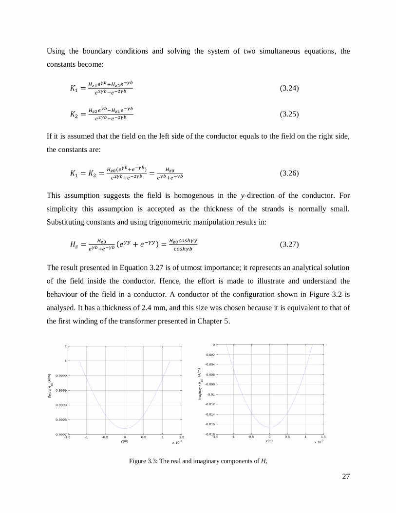
The result presented in Equation 3.27 is of utmost importance; it represents an analytical solution
of the field inside the conductor. Hence, the effort is made to illustrate and understand the
behaviour of the field in a conductor. A conductor of the configuration shown in Figure 3.2 is
analysed. It has a thickness of 2.4 mm, and this size was chosen because it is equivalent to that of
the first winding of the transformer presented in Chapter 5.
Figure 3.3: The real and imaginary components of Hz
-1.5 -1 -0.5 0 0.5 1 1.5
x 10-3
0.9997
0.9998
0.9998
0.9999
0.9999
1
1
y(m)
Rea
l x H
z0
-1.5 -1 -0.5 0 0.5 1 1.5
x 10-3
-0.018
-0.016
-0.014
-0.012
-0.01
-0.008
-0.006
-0.004
-0.002
0
y(m)
Imag
inar
y x
Hz0(A
/m)
(A/m
)

28
Figure 3.3 above depicts the results obtained from the calculation of the trigonometric functions
in Equation 3.27. The limits of the y dimensions are -1.2 mm to 1.2 mm. Thus the real and
imaginary components show a hyperbolic distribution at different positions of the conductor,
changing from the minimum to the maximum size. Furthermore, an important observation from
Figure 3.3 is that the magnitude of the real and imaginary components differs substantially.
Again at y equals to zero the extreme values are observed from both curves, the real showing the
minimum and the imaginary showing the maximum field.
Lastly, the resultant magnetic field expression in Equation 3.27 is principal to the calculation of
losses when combined with results of Poynting’s theorem detailed in the next section.
3.3. Power loss density
The theory encompassing the computation of the losses due to the time varying field has been
sufficiently developed. The physical definition of electromagnetic losses relies on Poynting’s
theorem. This theorem is widely applied to the cases of transmission lines. However according to
Franklin [42] the use of this theorem started long before it was formally defined as Poynting’s
theorem. In this publication he discusses the simplistic representation of the theorem using
current and voltage. Nonetheless, in this section the derivation of the theorem is provided.
According to Poynting’s vector, the loss density can be represented as the cross product of the
electric field and magnetic field.
(3.28)
The representation in Equation 3.28 is known as Poynting’s vector, which defines the loss
density according to the electromagnetic field quantities. The surface integral over the enclosed
surface of the same equation results in Equation 3.29.
The power losses are now:
∮
(3.29)
Therefore the mathematical representation of Poynting‘s theorem is:
∮
∮
∮
(3.30)
29
According to Equation 3.30, the total power equals to the sum of Ohmic losses and power
absorbed by the magnetic field. Hence, using the magnetic field and current density Equation
3.30 can be grouped in terms of the volume integral:
∮
∮
∮
(3.31)
The average power loss density is given by:
(3.32)
Where, is the complex conjugate of H. This relationship is illustrated in Equation 3.33 below.
[ ]
( ) (3.33)
Incorporating Equation 3.33, Poynting’s theorem in complex form becomes:
∮ | |
∮ | |
∮
(3.34)
On the basis of the one-dimensional approach, there exists only the x-component of the current
density and taking the real component of Equation 3. 34, the loss equation is:
∫ | |
(3.35)
This integral equation is vigorously applied in the next section. It is combined with the analytical
solution of the current density of the previous section.
3.4. One dimensional solution application
Using the diffusion equation and a solution from the boundary conditions of Equation 3.12, a
better definition of the current density is established. This current density is combined with the
integral equation of the Ohmic losses. In summary, the current density involves intricate
trigonometric functions. Thus, appropriate identities are applied to simplify the equation.
(3.36)
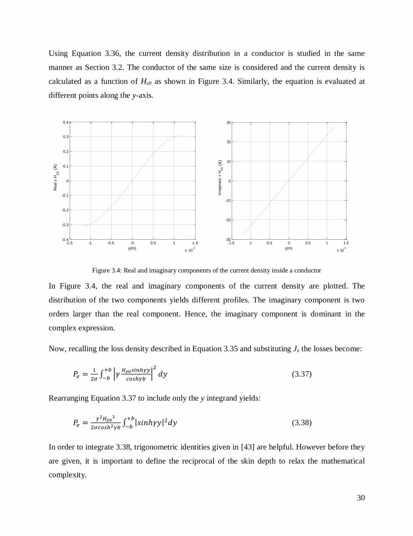
30
Using Equation 3.36, the current density distribution in a conductor is studied in the same
manner as Section 3.2. The conductor of the same size is considered and the current density is
calculated as a function of Hz0 as shown in Figure 3.4. Similarly, the equation is evaluated at
different points along the y-axis.
Figure 3.4: Real and imaginary components of the current density inside a conductor
In Figure 3.4, the real and imaginary components of the current density are plotted. The
distribution of the two components yields different profiles. The imaginary component is two
orders larger than the real component. Hence, the imaginary component is dominant in the
complex expression.
Now, recalling the loss density described in Equation 3.35 and substituting Jx the losses become:
∫ |
|
(3.37)
Rearranging Equation 3.37 to include only the y integrand yields:
∫ | |
(3.38)
In order to integrate 3.38, trigonometric identities given in [43] are helpful. However before they
are given, it is important to define the reciprocal of the skin depth to relax the mathematical
complexity.
-1.5 -1 -0.5 0 0.5 1 1.5
x 10-3
-0.4
-0.3
-0.2
-0.1
0
0.1
0.2
0.3
0.4
y(m)
Real x H
z0
-1.5 -1 -0.5 0 0.5 1 1.5
x 10-3
-30
-20
-10
0
10
20
30
y(m)
Imagin
ary
x H
z0(A
) (A)

31
√
(3.39)
From Equation 3.38 and 3.39, the trigonometric functions are simplified as follows:
| |
[ ] (3.40)
| |
[ ] (3.41)
Integrating (3.38) and substituting (3.40) and (3.41) the loss expression becomes
[ ]
[ ] (3.42)
Equation 3.42 is the loss density for both non-magnetic and magnetic materials. The relative
permeability of copper is 1 therefore copper can be treated as a non-magnetic material. To
analyse the relationship between the skin depth and strand sizes, it is important to simplify the
trigonometric functions. For the practical analysis, the conductor size limitations from the
manufacturers will constrain the dimensions. These limitations are the maximum and minimum
dimensions that the copper suppliers can manufacture. Hence, the data from three suppliers have
been displayed in Table 3.1. Before the assessment of Equation 3.42 is performed, the types of
conductors are described to enhance the understanding of the manufacturing limits.
Transformer windings are manufactured of copper strands insulated with paper or enamel. The
strands are laid out as edge wound or flat wound. The explanation of the two topologies follows.
Figure 3.5: Edge wound strand
Figure 3.5 shows the edge wound strand, from the transformer manufacturing perspective this
conductor configuration can only be used in a regulator winding. The latter applies specifically
for layer windings, due to the difficulties associated with the winding processes. The main
characteristic of this arrangement is that the b dimension is greater than the h dimension.
h
b

32
Figure 3.6: Flat wound strand
The flat wound strand is presented in Figure 3.6. This type of strand is not limited to applications
of any winding type. Its attribute as depicted in Figure 3.6 is that the b dimension is always
smaller than the h dimension. It has already been seen that the field in the conductor is
influenced by its thickness; in this section a meaningful assessment of the overall loss equation is
presented.
The main aim of the above discussion is to introduce the mechanical constraints surrounding the
conductor dimensions. Hence, the influence of the above configurations is assessed.
Furthermore, the comparison of a multitude of strand sizes and skin depth is presented.
Table 3.1: Supplier’s maxima and minima conductor dimensions
ASTA (mm) BTEW (mm) Aberdare (mm)
b Max 23 8 8
Min 2 0.8 1.5
h Max 7.5 21 35
Min 0.8 3.5 4
Courtesy of ASTA, BTEW and Aberdare
Consider the calculation of the skin depth of copper:
= 50 Hz
= H/m
= S/m
Substituting the above parameters in Equation 3.20 gives:
h
b
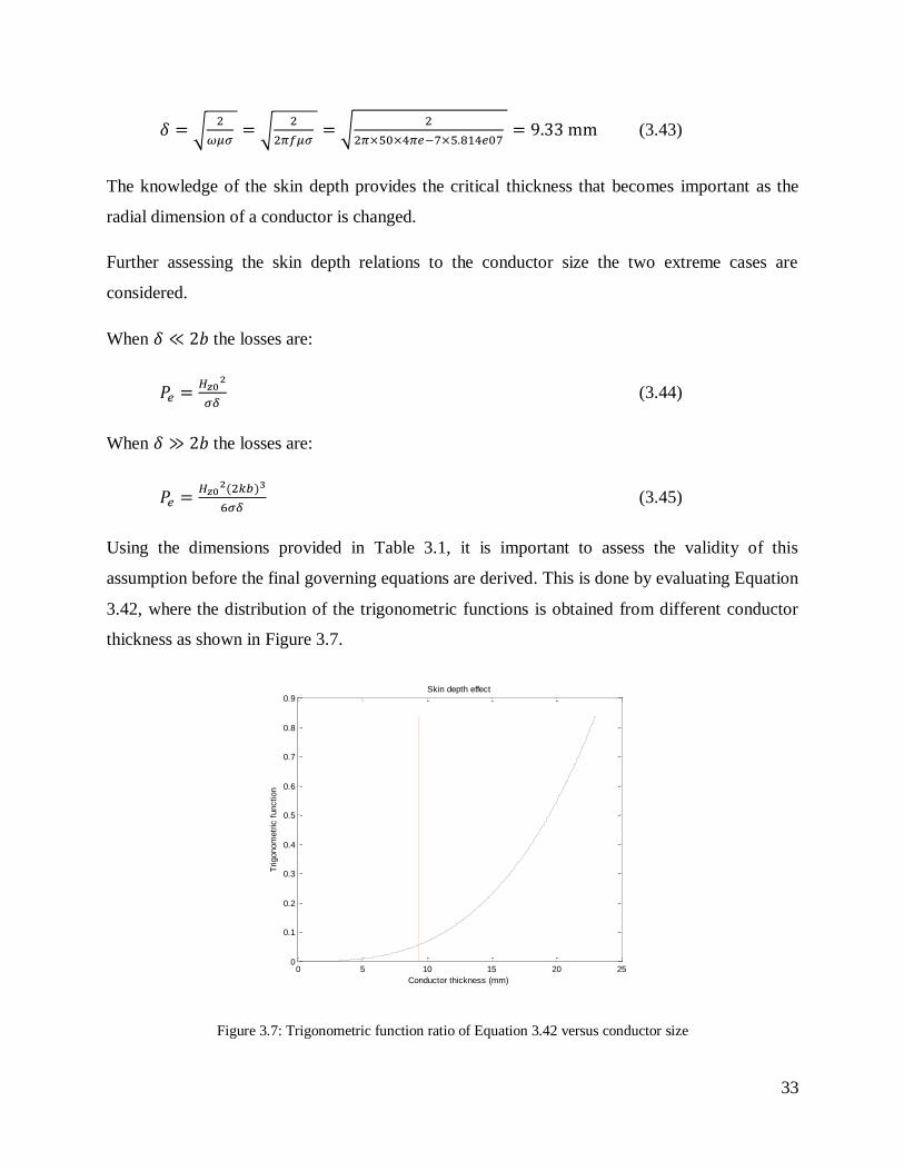
33
√
√
√
(3.43)
The knowledge of the skin depth provides the critical thickness that becomes important as the
radial dimension of a conductor is changed.
Further assessing the skin depth relations to the conductor size the two extreme cases are
considered.
When the losses are:
(3.44)
When the losses are:
(3.45)
Using the dimensions provided in Table 3.1, it is important to assess the validity of this
assumption before the final governing equations are derived. This is done by evaluating Equation
3.42, where the distribution of the trigonometric functions is obtained from different conductor
thickness as shown in Figure 3.7.
Figure 3.7: Trigonometric function ratio of Equation 3.42 versus conductor size
0 5 10 15 20 250
0.1
0.2
0.3
0.4
0.5
0.6
0.7
0.8
0.9Skin depth effect
Conductor thickness (mm)
Trigonom
etr
ic f
unction

34
Figure 3.7 presents the solution of the trigonometric part of Equation 3.42. Of this equation only
the trigonometric part is evaluated as it directly affects the earlier assumption. The maximum
size of 23mm of the conductor that can be supplied by ESTA as provided in Table 3.1 is used as
a guideline. The conductor size is then varied from 0.1 mm in steps of 0.001mm to assess the
trigonometric function. A total of 2291 points are obtained and plotted in Figure 3.7 against the
trigonometric function.
From Figure 3.7, there is a small variation of the function when the size of the conductor is less
than 5mm. From 5mm onwards the curve shows a rapid increase, roughly exponential. However
the critical point of this distribution is the cut-off between the plotted function and the skin depth
size that occurs at trigonometric function of 0.0551. The real meaning is that the losses are
enhanced by approximately
when the thickness of the conductor is equal to the skin
depth. Nonetheless, from the practical perspective this case can only occur on the regulator
winding when the edge wound conductor is used. If the regulator is designed using edge wound
and situated outside of the main field i.e. after the HV winding, the assumptions may still be
appropriate as a low quantity of winding eddy losses is expected.
The above analysis has shown that the assumption works well with small conductor thicknesses,
once the conductor size becomes larger than 5mm the losses can be overestimated. This
assumption is therefore limited to small conductor sizes.
Proceeding with the derivation, let t=2b be a conductor thickness, and substitute t into Equation
3.45 to get:
√
√
√
(3.46)
The above expression can be represented in terms of the flux density and as losses per unit
volume according to:
(3.47)
B0 is the peak flux density.

35
The flux density has axial and radial components, if that is taken into account, Equation 3.47
above can be split into the respective components and perpendicular surface as:
(3.48)
(3.49)
In Equation 3.48 and 3.49, is the axial flux density and is the radial flux density component
respectively.
Before Equation 3.48 and 3.49 are accepted and used to evaluate the winding eddy losses of the
transformer, it is important that at this stage their local accuracy requirement is understood. As a
result, a 2-D FEM simulation of a single conductor is performed in Ansoft Maxwell. The aim is
to determine the winding eddy losses in twofold, those are to:
a) Use the mid-flux density value and apply Equation 3.48 and 3.49.
b) Use the flux density per mesh element, integrate and apply Equation 3.48 and 3.49.
With the geometry, boundary and current density values provided in Appendix A, losses are
calculated using the two methods a) and b). For the purposes of the calculation of losses, the
copper conductivity of 47.303 MS/m is used. This is the conductivity of the copper material as
obtained at a reference temperature of 75°C as discussed in Chapter 6.
The results of the simulation are as follows:
Using the first option a) the losses are: Pa = 3.4214 W and Pr = 0.210 W
Using the first option b) the losses are: Pa= 3.483 W and Pr = 0.7997 W
From the simulation results presented above the difference obtained when comparing the axial
component is 1.78%, meanwhile the radial component difference is 73.69%. It can be deduced
that the simplification of Equation 3.49 is not adequate for the evaluation of the radial winding
eddy losses. In addition, to understand this further a parametric study of how the field varies with
the thickness of the conductor is shown in Figure 3.8. The table of the input values of the
parameters that changed during the study is shown in Appendix A.
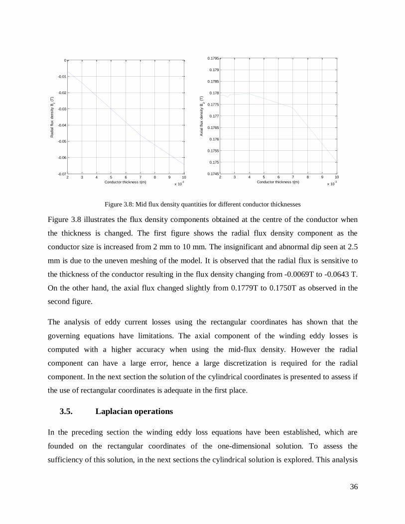
36
Figure 3.8: Mid flux density quantities for different conductor thicknesses
Figure 3.8 illustrates the flux density components obtained at the centre of the conductor when
the thickness is changed. The first figure shows the radial flux density component as the
conductor size is increased from 2 mm to 10 mm. The insignificant and abnormal dip seen at 2.5
mm is due to the uneven meshing of the model. It is observed that the radial flux is sensitive to
the thickness of the conductor resulting in the flux density changing from -0.0069T to -0.0643 T.
On the other hand, the axial flux changed slightly from 0.1779T to 0.1750T as observed in the
second figure.
The analysis of eddy current losses using the rectangular coordinates has shown that the
governing equations have limitations. The axial component of the winding eddy losses is
computed with a higher accuracy when using the mid-flux density. However the radial
component can have a large error, hence a large discretization is required for the radial
component. In the next section the solution of the cylindrical coordinates is presented to assess if
the use of rectangular coordinates is adequate in the first place.
3.5. Laplacian operations
In the preceding section the winding eddy loss equations have been established, which are
founded on the rectangular coordinates of the one-dimensional solution. To assess the
sufficiency of this solution, in the next sections the cylindrical solution is explored. This analysis
2 3 4 5 6 7 8 9 10
x 10-3
-0.07
-0.06
-0.05
-0.04
-0.03
-0.02
-0.01
0
Conductor thickness t(m)
Radia
l flux d
ensity B
r (T
)
2 3 4 5 6 7 8 9 10
x 10-3
0.1745
0.175
0.1755
0.176
0.1765
0.177
0.1775
0.178
0.1785
0.179
0.1795
Conductor thickness t(m)
Axia
l flux d
ensity B
z (
T)

37
is governed by the cylindrical representation of the Laplacian operator. The difference between
the scalar and vector Laplacian is not recognized through many textbooks [44]. The lack of
understanding thereof leads to many assuming that these two are easily transformed from the
rectangular coordinate system to the cylindrical coordinate system. Nevertheless the vector
Laplacian operation is not as comprehensible as the scalar potential; hence the fundamental
differences are explicitly outlined. In addition, the eddy current problems demand that the former
is properly understood; accordingly this section provides the distinction of the two expansions in
differential form as contained in [44].
The cylindrical scalar Laplacian:
(3.50)
The cylindrical vector Laplacian:
[
]
[
]
[
]
(3.51)
3.6. Eddy current solution in cylindrical coordinates
The traditional one-dimensional solution presented in preceding sections is based on rectangular
coordinates and does not take the curvature into consideration. In this section Maxwell’s
equations are solved using the cylindrical description of the field. The work presented is derived
from first principles; in addition the cylindrical solution has been presented in [3] when dealing
with conducting tubes to screen the solenoid conductors. Furthermore, Figure 3.9 illustrates the
winding conductor orientation in cylindrical coordinates. It is clear that the curvature needs to be
accounted for with minimal assumptions. The consideration of the curvature may however lead
to an intricate mathematical solution of the diffusion equation.

38
Figure 3.9: Cylindrical setup of the conductor, placed in the magnetic field
Consider Equation 3.51:
[
]
[
]
[
]
(3.52)
The diffusion equation appears complex, in this equation the magnetic field is applied in
cylindrical form using the Laplacian operation explained in Section 3.7.
However, from Figure 3.9, similar to the rectangular coordinates, it is established that the eddy
current flows in the φ direction such that; .
It is further assumed that the magnetic field has only the z-component changing in the r-
direction. Hence, it is deduced that:
[
]
(3.53)
The partial definition can be dropped since there is only the z-component of the field, rewriting
3.53 results in:
(3.54)

39
The solution of the above diffusion equation does not have a simple general equation. For
simplicity, it is essential to express this equation in the frequency domain as follows:
(3.55)
Let
(3.56)
The solution of this equation satisfies modified Bessel functions of zero order [45], thus the
solution becomes:
(3.57)
A and B are arbitrary constants determined using the knowledge of boundary conditions. To
explain the boundary values, Figure 3.10 is presented.
Figure 3.10: Top view of the cylindrical layout of the winding
From Figure 3.10 the boundary conditions result in Equations 3.58 and 3.59 below
(3.58)
(3.59)
Given the small thickness of the winding strands, it makes sense to assume equals to to
become . Hence, solving Equation 3.58 and 3.59 simultaneously yields:
(3.60)
r=b1
r=b0
Hz2
Hz1

40
Substituting 3.60 into 3.59 yields:
[ ]
(3.61)
Now, it is important to obtain the solution of A:
[ ]
(3.62)
Simplifying 3.62 results in:
[ ]
(3.63)
Both solution constants are now shown as only dependent on Modified Bessel functions. So it
becomes practical to replace them back into Equation 3.57, yielding:
[ [ ]
]
[ [ ]
] (3.64)
Now that the solution of the field is simplified, it is required to represent Equation 3.2 in
cylindrical coordinates, and solve the determinant as shown in Equation 3.65:
|
| (3.65)
The solution from the problem definition explained above results in the current density of:
(3.66)
At this stage the magnetic field solution is known. It is therefore substituted back into Equation
3.66. This solution is now in differential form and the current density is attainable.
[ [
[ ]
]
[ [ ]
]]
(3.67)

41
The derivative of Equation 3.67 cannot be calculated using conventional methods, hence the
identities are recalled:
(3.68)
(3.69)
Equation 3.68 and 3.69 are derivatives of the first and second kind of the Modified Bessel
functions found in [46]. The order of these expressions is represented by v; substituting the actual
order they are:
(3.70)
(3.71)
It is apparent that the derivative of the zero order is equal to the first order of the Modified
Bessel function for both the first and second kind.
Taking the derivative of Equation 3.67 through the combination of identities presented above
yields:
[( [ ]
)
( [ ]
)
] (3.72)
With the purpose of understanding the true meaning of expression 3.72, the current density is
assessed with respect to r. This parameter is constrained within the inner radius and the
thickness of the conductor. Evoking the material properties of copper that have been provided,
the terms containing r are evaluated. Furthermore, β is a complex function with real and
imaginary components. For the computational purposes both real and imaginary components are
considered during the evaluation of the Modified Bessel functions. Now, using a Matlab
calculation routine, the current density distributions illustrated in Figure 3.11 and Figure 3.12
are obtained.

42
Figure 3.11: Current density distribution within a 2mm conductor
Figure 3.12: Current density distribution within a 5mm small conductor
The results presented in Figure 3.11 and Figure 3.12 are based on a 500mm winding inner radius;
it is also separately proved that there is no change of the distribution when a smaller inner radius
of 200mm is considered. The choice of the inner radius is due to average practical dimensions of
transformer windings.
The direct proportionality between the magnetic field and the current density allows for an
assessment of the current density as a function of magnetic field. Thus the 2mm and 5mm
conductor sizes are analysed and the results show a linear distribution of the current density
across the thickness of the conductor. The current density distribution is symmetrical and almost
zero at the centre of the conductor.
The smaller conductor sizes have shown a linear distribution, however a larger sized conductor
of 23mm derived from the Table 3.1 shows a periodic distribution. The latter was amplified
arbitrarily by considering a 50 mm thick conductor where the distribution is obviously periodic
as shown in Figure 3.13 and Figure 3.14.
0.5 0.5005 0.501 0.5015 0.502 0.5025-0.4
-0.3
-0.2
-0.1
0
0.1
0.2
0.3
Winding inner radius(m)
Real curr
ent
density a
s (
Hz0)
Current density distribution (Conductor thickness=2mm)
0.5 0.5005 0.501 0.5015 0.502 0.5025-0.4
-0.3
-0.2
-0.1
0
0.1
0.2
0.3
Winding inner radius(m)
Imagin
ary
curr
ent
density a
s (
Hz0)
Current density distribution (Conductor thickness=2mm)
0.5 0.501 0.502 0.503 0.504 0.505 0.506-0.8
-0.6
-0.4
-0.2
0
0.2
0.4
0.6Current density distribution (Conductor thickness=5mm)
Winding inner radius (m)
Real curr
ent
density a
s (
Hz0)
0.5 0.501 0.502 0.503 0.504 0.505 0.506-0.8
-0.6
-0.4
-0.2
0
0.2
0.4
0.6Current density distribution (Conductor thickness=5mm)
Winding inner radius (m)
Imagin
ary
curr
ent
density a
s (
Hz0)

43
Figure 3.13: Current density distribution within large conductors (23mm)
Figure 3.14: Current density distribution within large conductors (50mm)
The analysis of the different conductor sizes shows that the imaginary component decreases as
the conductor thickness is increased. The real component of the larger conductor shows a rapid
reduction of the current density at the centre of the conductor. This is due to the inherent skin
effect of the conductor. With the complete understanding of the distribution of the current
density in Figure 3.11, Figure 3.12, Figure 3.13 and Figure 3.14, the focus shifts to its relation to
the formulation of the Ohmic losses defined in Section 3.3. Thus, recalling Equation 3.7 and
substituting the new current density yields:
∫ |
[( [ ]
)
( [ ]
)
]|
(3.73)
0.5 0.505 0.51 0.515 0.52 0.525-3
-2
-1
0
1
2
3Current density distribution (Conductor thickness=23mm)
Winding inner radius (m)
Real curr
ent
density a
s (
Hz0)
0.5 0.505 0.51 0.515 0.52 0.525 0.53-0.4
-0.3
-0.2
-0.1
0
0.1
0.2
0.3Current density distribution (Conductor thickness=23mm)
Winding inner radius (m)
Imagin
ary
curr
ent
density a
s (
Hz0)
0.5 0.51 0.52 0.53 0.54 0.55 0.56-2
-1.5
-1
-0.5
0
0.5
1
1.5
2Current density distribution (Conductor thickness=50mm)
Winding inner radius (m)
Real curr
ent
density a
s (
Hz0)
0.5 0.51 0.52 0.53 0.54 0.55 0.56-0.8
-0.6
-0.4
-0.2
0
0.2
0.4
0.6
0.8Current density distribution (Conductor thickness=50mm)
Winding inner radius (m)
Imagin
ary
curr
ent
density a
s (
Hz0)

44
The above equation looks tedious; to simplify it the following constants are defined:
(
) (3.74)
(
) (3.75)
Rearranging the like terms, the losses become:
[ ∫ |
|
∫ |
|
] (3.76)
It appears that the solution of Equation 3.76 is transcendental in a sense that it requires laborious
mathematical manipulations. An attempt is made to solve it using computational platforms such
as Matlab and Mathematica. This is done by computing each term as detailed below.
For further comprehension, the analysis of the integration terms is conducted. In addition, the
integration of the square of the Modified Bessel of the second kind function of first order proved
to be impossible in Matlab. This immediately prompted the use of the mathematically focused
software, which is Mathematica. The added advantage of this software is the ability to specify
the machine precision deemed sufficient.
Figure 3.15: Integration of Modified Bessel functions at 500 mm radius
0.5 0.505 0.51 0.515 0.52 0.525 0.530
0.2
0.4
0.6
0.8
1
1.2
1.4
1.6
1.8
2x 10
21 Conductor thickness (23 mm)
Winding radius (m)
C0*I
nt(
(I1(x
)/x)2
)
0.5 0.505 0.51 0.515 0.52 0.525 0.53-6
-4
-2
0
2
4
6x 10
53
Winding radius (m)
D0*
Int((
K1(
x)/(x
))2
Conductor thickness (23 mm)

45
Figure 3.16: Integration of Modified Bessel functions at 200 mm radius
Using the knowledge of the maximum conductor sizes specifically the thickness; the integral
terms are assessed while varying the conductor thickness. The investigation is done separately
using the two inner radii values namely; 500 mm and 200 mm. It is observed from both Figure
3.15 and Figure 3.16 that the first term diverges as the conductor size increases. It is also notable
that the order of the y-axis value reduces rapidly when the radius is 200 mm, indicating a
dependency on the inner radius. The second term is also not sensible as there is visible distortion
as soon as the conductor thickness exceeds skin depth. If the results were valid, the investigation
similar to Section 3.4 would have been pursued.
The Author is of the view that the cylindrical approach is difficult to provide important and valid
results. The anomalies suggest that this detailed approach is too complex for practical
transformer applications. In addition, it is known that design routine programs significantly
demand the relaxation of mathematical complexity. Hence the use of the cylindrical one-
dimensional approach is not justifiable. Notwithstanding that the apparent behaviour may
suggest that at smaller inner radii and conductor sizes, Equation 3.76 may be of practical use,
there may be applications for this approach outside transformers. The method can in future be
investigated further to quest for the identities that may simplify the integration of Modified
Bessel functions.
0.2 0.205 0.21 0.215 0.22 0.2250
2
4
6
8
10
12
14
16
18x 10
7 Conductor thickness (23 mm)
Winding radius(m)
C0*I
nt(
(I1(x
)/x)2
)
0.2 0.205 0.21 0.215 0.22 0.225-4
-3
-2
-1
0
1
2
3
4
5x 10
12 Conductor thickness (23 mm)
Winding radius(m)
D0*I
nt(
(K1(x
)/x)2
)

46
3.7. Conclusion
This chapter focused on the derivation of winding eddy losses using rectangular and cylindrical
coordinate solutions. The rigorous approach to eddy current loss computation using cylindrical
coordinates has been derived. It however proves to be mathematically impractical as the
integration of the Modified Bessel functions yields insoluble results.
Winding eddy loss equations obtained in Equations 3.48 and 3.49 remain the key governing
equations for the computation of winding eddy losses. The two equations show that the
respective loss components are directly proportional to the square of the incident flux density
components. Hence, there is a need to accurately evaluate these flux density components.
Furthermore there is a large error in the magnitude of 74% associated with the radial loss
component. It can be deduced that the simplifications applied for Equation 3.49 are inadequate
for the evaluation of the radial winding eddy losses. The integration resolution should be
improved, which is done in the computation of winding eddy losses using 3-D FEM in Chapters
5 and 6. The next chapter explores in detail the method of computing the flux density
components as well as selecting the method that is significant in accurately predicting the
winding eddy losses.

47
Chapter 4
Evaluation of Rabins’ analytical method
In Chapter 3, the computation formulae for winding eddy losses are established. Inherently, the
winding eddy loss components are governed by the incident radial and axial flux densities. These
two equations are derived from the one-dimensional behaviour of the field using rectangular
coordinates which are considered adequate. The losses are proportional to the square of the
incident field. Accordingly, in the event that the field is incorrectly evaluated the resulting error
is squared. In this chapter, the rigorous and practical methods essential to the determination of
the field quantities are explored. In particular, the analytical method is sought, this done by
critically assessing known methods and juxtaposing them against the numerical method.
The method of determining the field distribution in transformers was first introduced by
Rogowski. An account of his work is given by Hague [47]; a section is dedicated to the treatment
of the leakage fields using this method. Rogowski was concerned with the evaluation of leakage
field and reactance of sandwich windings. The leakage flux problem is treated in rectangular
coordinates such that the windings are assumed long bars. The periodic distribution of the field
allowed for the representation of the distribution using a single Fourier series. However, the main
shortcoming of Rogowski’s work is the inability to take the curvature of the windings into
account.
48
The next person to improve the calculation of the leakage field distribution was Roth. He
published a series of papers from 1927, mainly to address the leakage flux computations. His
first publication dealt with the flow of heat in electrical machinery, later the mathematic
similarity to magnetic problems was observed. Instead of separating the vector potential regions
like Rogowski, Roth expresses the solution of the non-current carrying sections in a universal
manner. This vector potential approach satisfies the double Fourier series in the x-y system. In
addition, Hague praises Roth by saying that his [Roth] papers are a complete treatise which no
student of these problems can ignore [47]. Interestingly, later on Hammond [50] argues that
Hague commits a mistake by using the word treatise. He outlines the limitations of Roth’s
method, which are chiefly attributed to complex formulations.
It can be said however that Hammond’s dispute of Hague’s praises is unfair to a certain degree.
The fact that he published his work after researchers had already advanced the subject meant
added resources. One such is Billing. In 1951 [51], he published a paper to calculate the
magnetic field in rectangular conductors. His solution of magnetic vector potential was based on
Fourier series and Bessel functions; he therefore extended the earlier work of Rogowski and
Roth. The remarks of this work include the magnetic vector potential mapped everywhere in the
core window. However, the discrepancy of this method is the assumption of axial symmetry and
neglecting of the curvature.
To take the curvature into account a breakthrough was witnessed in 1956, this is when Rabins
advanced the calculation of flux densities using analytical methods. In addition, this method
appears in the publication by Thomson [48], which seems to be earlier than Rabins.
Nevertheless, the method is now known as Rabins’ method, Del Vecchio et al [43] have a
complete section entitled “Rabins Method for Calculating Leakage Fields, Forces, and
Inductance in Transformers”. The advantage of Rabins’ method is the rigorous analytical
approach towards obtaining the solution of the magnetic vector potential in cylindrical
coordinates. This is done by expressing the solution of the field in cylindrical coordinates using
Modified Bessel, Struve and Fourier series functions. In [49], Rabins presented his method
primarily to calculate the leakage reactance of power transformers using digital computers.
Nowadays, computers are fast, perpetuating the need for relaxing assumptions tailored for digital
computers. Meanwhile, mathematics packages such as Matlab and Mathematica come with
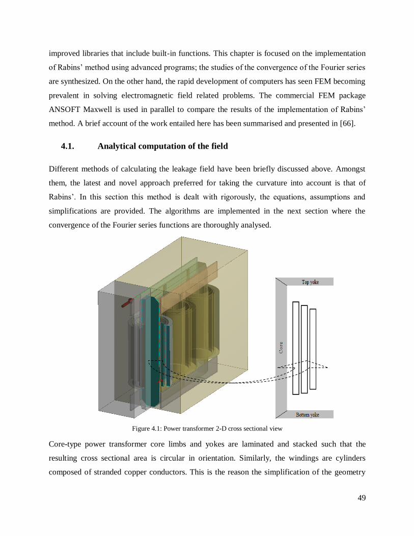
49
improved libraries that include built-in functions. This chapter is focused on the implementation
of Rabins’ method using advanced programs; the studies of the convergence of the Fourier series
are synthesized. On the other hand, the rapid development of computers has seen FEM becoming
prevalent in solving electromagnetic field related problems. The commercial FEM package
ANSOFT Maxwell is used in parallel to compare the results of the implementation of Rabins’
method. A brief account of the work entailed here has been summarised and presented in [66].
4.1. Analytical computation of the field
Different methods of calculating the leakage field have been briefly discussed above. Amongst
them, the latest and novel approach preferred for taking the curvature into account is that of
Rabins’. In this section this method is dealt with rigorously, the equations, assumptions and
simplifications are provided. The algorithms are implemented in the next section where the
convergence of the Fourier series functions are thoroughly analysed.
Figure 4.1: Power transformer 2-D cross sectional view
Core-type power transformer core limbs and yokes are laminated and stacked such that the
resulting cross sectional area is circular in orientation. Similarly, the windings are cylinders
composed of stranded copper conductors. This is the reason the simplification of the geometry
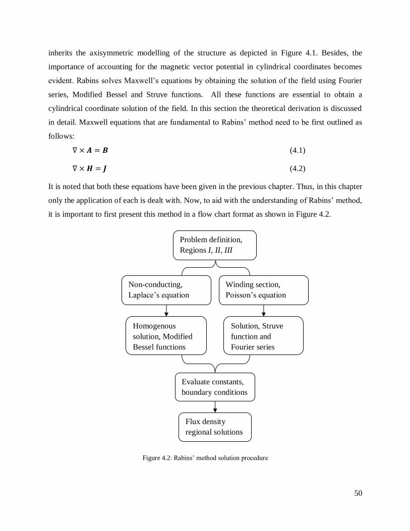
50
inherits the axisymmetric modelling of the structure as depicted in Figure 4.1. Besides, the
importance of accounting for the magnetic vector potential in cylindrical coordinates becomes
evident. Rabins solves Maxwell’s equations by obtaining the solution of the field using Fourier
series, Modified Bessel and Struve functions. All these functions are essential to obtain a
cylindrical coordinate solution of the field. In this section the theoretical derivation is discussed
in detail. Maxwell equations that are fundamental to Rabins’ method need to be first outlined as
follows:
(4.1)
(4.2)
It is noted that both these equations have been given in the previous chapter. Thus, in this chapter
only the application of each is dealt with. Now, to aid with the understanding of Rabins’ method,
it is important to first present this method in a flow chart format as shown in Figure 4.2.
Figure 4.2: Rabins’ method solution procedure
Homogenous
solution, Modified
Bessel functions
Non-conducting,
Laplace’s equation
Problem definition,
Regions I, II, III
Winding section,
Poisson’s equation
Solution, Struve
function and
Fourier series
Evaluate constants,
boundary conditions
Flux density
regional solutions

51
Figure 4.2 shows the typical procedure followed in the implementation of Rabins’ method. As
already mentioned in the introductory section of this chapter, this method is used to evaluate the
leakage field between the transformer windings and subsequently the local flux density
components. The first step is to envisage a cross sectional view presented in Figure 4.1. In this
step the horizontal ducts and the winding that lie inside the core window are denoted as regions I,
II, III. These regions become the cornerstone of the implementation of Rabins’ method as the
magnetic vector potential of each is sought.
The second step is to use the appropriate Maxwell’s equations and express them in cylindrical
coordinates to take the curvature into account. This step seeks to represent field equations in
terms of the current density and the magnetic vector potential. At this point the field and current
distributions should be visualised as conforming to periodic functions. It follows that the core
and duct regions have no source current density. Hence, the two equations Laplace and Poisson
are introduced.
Step three searches for the general solution of the two equations. In addition, the solution of
partial differential equations of the cylindrical coordinate inherits Modified Bessel functions. In
the respective regions, if there is a current source that is spatially distributed, the solution
includes Modified Struve functions.
Once the equations are solved, the integration constants become the new unknowns. The
boundary conditions are then used to determine these constants. Lastly, they are substituted back
into the magnetic vector potential solutions of the different regions. The analytical equations are
then manipulated to give the solution of the local flux density components. Lastly, most sections
of this chapter are devoted to describing the individual aspects presented in Figure 4.2.
In order to accomplish the whole implementation of Rabins’ method, the assumptions that
constrain the behaviour of the field are required. They are particularly applied to determine the
constants, these assumptions are:
Infinite permeability of the core.
The yokes are infinitely large.
The ampere-turn unbalance is approximately zero.
The effect of the tank wall and adjacent windings is negligible.

52
To proceed with the derivation Equation 4.1 is substituted into Equation 4.2 and combining them
with the relationship between the magnetic field and flux density produces:
(4.3)
Equation 4.3 can be expanded to obtain the following:
(4.4)
Through vector operations described in Chapter 3, Equation 4.4 yields:
(4.5)
Considering that the winding is cylindrically constructed as outlined above, it can be deduced
that the current flows only in the azimuthal direction; Figure 3.9 in Chapter 3 depicts this
phenomenon, hence:
(4.6)
In Equation 4.6 the term has been dropped because the permeability of copper is
approximately 1. Furthermore, the result of Equation 4.6 is a significant one in that it postulates
that the component of the magnetic vector potential required in the winding is only in the
azimuthal direction, giving the expression below.
(4.7)
The expression shown in Equation 4.7 is the Laplacian operator of the vector potential in
cylindrical coordinates. In addition, the terms containing the changing magnetic vector potential
in the azimuthal direction are eliminated since the solution is axisymmetric. The remaining
components of the field are those that change in the r and z directions. Following this
explanation, the regional solutions are diagrammatically depicted below. The aim is to clearly
establish the non-current and current carrying solutions so as to distinctly represent them in an
analytical manner.

53
Figure 4.3: Transformer core and winding arrangement
In Figure 4.3 the following boundaries are established:
Region I ≤ r ≤ , 0 ≤ z ≤ L
Region II ≤ r ≤ , ≤ z ≤
Region III r > ≤ 0 ≤ z ≤ L
The classification of boundaries in Figure 4.3 and the simplification of Equation 4.6, results in
the following magnetic vector potential expressions:
Region I and III:
(4.8)
Region II:
(4.9)
Equation 4.9 is the partial differential equation of Poisson’s form that defines the problem that
Rabins is credited for solving using a mathematically manageable solution. He introduced the
Winding
Top Yoke
Bottom Yoke
Core limb
Br

54
Struve function term while satisfying periodic distribution. The diagram shown in Figure 4.4
illustrates the harmonic current distribution that will aid in the understanding of the problem.
Figure 4.4: Distribution of current density along the window section
The multi-coils presented in Figure 4.4 show that in the axial direction the current distribution
can be represented as a piece wise function. In addition, in Chapter 3 it is demonstrated that the
distribution of the current density in a conductor is periodic. Even though the study was based on
the radial direction, it is also applicable to the distribution of current in the axial direction. In this
case, each coil resembles the harmonic distribution. Thus, for the practical examples used in this
dissertation, it is accepted that the current distribution of a single coil satisfies the spatial
formulation. The interval of this periodic representation is defined by the core window height L
as shown in Figure 4.4. This concept is abstract and an extended explanation is found in [52].
Boyajian discusses the harmonic concept of the current density distribution in the core window
Axia
l

55
of a transformer. Furthermore, the work of Rogowski is premised on sandwiched winding
arrangements, where the periodic distribution of the current density is outlined. As shown in
Figure 4.4, the assumption is that the current is uniform in each section satisfying:
∑ (4.10)
Assuming that the magnetic vector potential is distributed in a periodic manner as is the current
density, it becomes:
∑ (4.11)
Where:
(4.12)
In Equation 4.12, n denotes the index of the number of series elements equal to 1, 2, 3... The
winding can be separated into numerous segments, each having a uniform current distribution.
The region of interest in this analysis is II; and satisfies the spatial current distribution as
explained above. However the solution of region I and II are first discussed.
From Figure 4.3 the regions I and III have zero source current density. Hence, the magnetic
vector potential solution of this equation becomes homogenous. This further permits the
expression of the product of R(r) and Z(z) as a function of separation of variables [53].
(4.13)
Dividing by R(r) Z(z) yields,
(4.14)
To find the solution of Equation 4.14, the different coordinates need to be segregated. This is
done by assuming that the sum of the square of a constant equals to zero. Therefore the r
component becomes
(4.15)
Subsequently the z term follows:
(4.16)

56
m has two possibilities i.e. m=0 or m>0, the independent solutions of m are therefore sought for
both R and Z.
Solving for R when m =0 yields:
(4.17)
The general solution of Equation 4.17 is vastly known in the field of mathematics,
(4.18)
When m > 0, solving for R and Z.
(4.19)
(4.20)
The vector potential solution of regions I and II is simplified by substituting the R and Z
solutions in Equation 4.19 and 4.20 respectively and, the magnetic vector potential becomes:
∑ [ ]
(4.21)
We change focus to the magnetic vector potential solution of region II, in this instance the
harmonic distribution is substituted into the differential Equation 4.9. It follows that the solution
satisfying Equation 4.22 is sought:
∑ (4.22)
From Equation 4.21, the z component immediately becomes:
∑
∑ (4.23)
The above mathematical manipulation is necessary to eliminate the z component. Substituting
Equation 4.23, 4.24 and 4.10 into 4.9 results in:
∑ [
]
∑
[ ∑ ] (4.24)
For n=0 and considering like terms yields:
(4.25)

57
Therefore the general solution becomes:
(4.26)
When n > 0, Equation 4.24 becomes:
∑[
]
∑
∑
(4.27)
The orthogonality of the cosine function allows for the dropping of the Fourier series
representation and Equation 4.27 is simplified to:
(4.28)
Similar to Equation 4.20, the particular solution of R satisfies Modified Bessel functions, but
now a new term, Modified Struve function of order one is introduced.
(4.29)
Substituting the solutions back into 4.21, the following is obtained:
∑ [
]
(4.30)
If the same approach as in Equation 4.7 is used and Equation 4.1 is evaluated, the following
point flux densities are obtained:
(4.31)
(4.32)
Thus from differentiating Equation 4.32 by parts, we get
(4.33)
The next step is to obtain the solution constants of the three regions as shown in Figure 4.3.
Within these regions, the following field boundary conditions need to be satisfied:

58
The components of the field have to be continuous at the region interface, thus
o Flux density
At r = r1 BrI = Br
II
At r = r2 BrII
= BrIII
o Magnetic field
At r = r1 HzI = Hz
II
At r = r2 HzII
= HzIII
The radial flux density component at equals to zero, i.e. infinite permeability of the
core
o
=0
The boundary conditions outlined above are pivotal to the determination of the solution
constants. Using the magnetic vector potential solutions of the regions, the constants are
evaluated; this process is extensively covered in [47],[48],[49],[50],[51],[43]. As a result, only
the computational aspect of the constants is covered in this section.
To ease the mathematical representation, , for n =1,2,… as already defined above is used.
Even though the process is not given here, eventually five constants are defined. They are Cn, Dn,
En, Fn and Gn. These constants are mainly dependent on the geometric parameters. They are
evaluated using the transformer data provided in Appendix B. In this section they are all plotted
except Gn. The omission of Gn becomes obvious in the following sections. The number of terms
of the series is restricted to 70 in the evaluation of constants.
∫
(4.34)
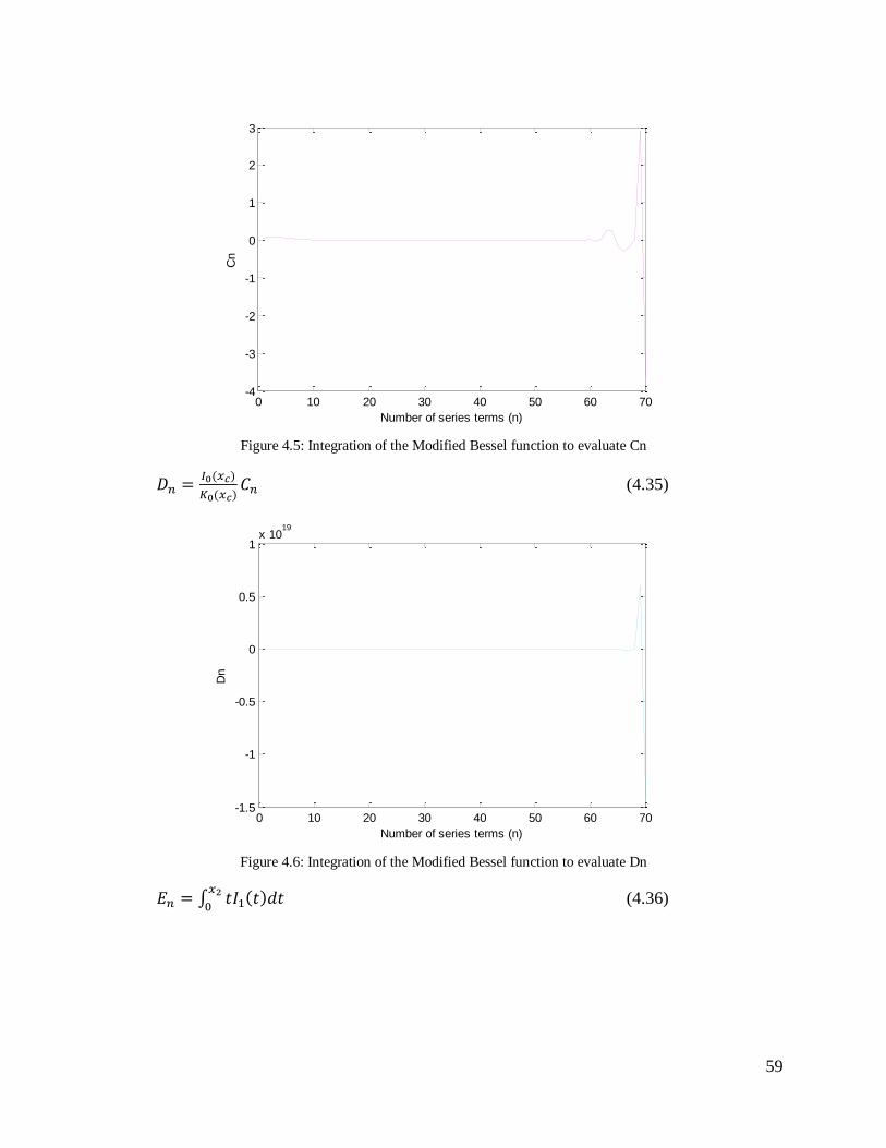
59
Figure 4.5: Integration of the Modified Bessel function to evaluate Cn
(4.35)
Figure 4.6: Integration of the Modified Bessel function to evaluate Dn
∫
(4.36)
0 10 20 30 40 50 60 70-4
-3
-2
-1
0
1
2
3
Number of series terms (n)
Cn
0 10 20 30 40 50 60 70-1.5
-1
-0.5
0
0.5
1x 10
19
Number of series terms (n)
Dn

60
Figure 4.7: Integration of the Modified Bessel function to evaluate En
∫
∫
(4.37)
Figure 4.8: Integration of Modified Bessel functions to evaluate Fn
Of the shown constants above, Cn and En are observed to consist of consumable values. In
particular, Cn is seen to have a smooth convergence after a few n-terms. On the contrary, Dn and
Fn have very high exponent values. At this stage however these values are not of concern. The
typical expectation is that these exponents get compensated for by the corresponding terms.
0 10 20 30 40 50 60 700.4
0.6
0.8
1
1.2
1.4
1.6
1.8
Number of series terms (n)
En
0 10 20 30 40 50 60 70-0.5
0
0.5
1
1.5
2
2.5x 10
16
Number of series terms (n)
Fn

61
Having obtained and plotted the behaviour of the solution; it is a good position to determine the
vector potential solutions of all the regions.
∑
[ ] (4.38)
(
) ∑
[
]
(4.39)
∑
(4.40)
The flux density components are obtained from substituting Equation 4.31 and 4.33 into the
simplified vector potential solutions above. The local flux density components of region II are
given by Equations 4.41 and 4.42.
∑
[
] (4.41)
∑
[
]
(4.42)
The transformer used for the implementation of the analytical approach consists of two windings.
For this situation, it is of utmost importance to realize the need to superimpose the solution for
regions I and II for any point in winding A. Hence, the actual flux density value is the sum of the
two solutions.
Thus the superposition of regions I and II yields:
[
]
[ ]
(4.43)
[
]
[ ]
(4.44)
The two equations presented above are important in this chapter; as the next section discusses
how they are implemented in a computer program.

62
4.2. Rabins’ algorithm implementation
The derivation of Rabins’ method has been discussed in the preceding section, now this
algorithm needs to be implemented in mathematical programs. At the time Rabins developed the
method, he used digital computers to evaluate the Fourier series expansion terms. With
awareness of convergence limitations, asymptotic approximations were introduced to correctly
approximate Modified Bessel and Struve functions. Today, a variety of computational platforms
are available, the discussion in this section is focused on using two platforms namely; Matlab
and Mathematica.
The initial attempt to implement Rabins’ algorithms was initiated in Matlab where Modified
Bessel and Struve functions were evaluated as part of the Fourier series expansion. This package
however proved to be insufficient in terms of controlling the number of digits of precision of the
solution. The main observations include divergence when high order harmonics of the Fourier
series expansions are considered. Terms exceeding forty were already showing divergence. The
main cause of this phenomenon is the outward calculation approach inherent to Matlab
operations. In this instance, the precision is sequentially lost in every execution step. This
dependence immediately prompted a need for a more robust platform; with a flexible number of
digits of precision.
From the above explanation, the package available to explore the precision requirements is
Mathematica. In this section the implementation of Rabins’ algorithms is entailed. The effect of
the number of digits of precision versus accuracy is extensively analysed. In addition, the
number of terms sufficient to obtain convergence is rigorously assessed.
The geometry dimensions and characteristics of the transformer used for the study are provided
in Appendix B. This transformer is used throughout the chapter for all comparisons.
4.2.1. Assessment of the number of digits of precision
The flux density components are calculated at the centre of the radial position (fixed) of the
winding. Along the winding height, the axial position is increased in step increments equal to the
conductor height in order to discretize the winding into several strands of centroid coordinates.
In determining the sufficient number of digits of precision an assumption of 70 Fourier series
elements is considered. The assumption was also made by Kulkarni [9]; he states that the
mentioned number suffices, notwithstanding the detailed validation in the next section. The
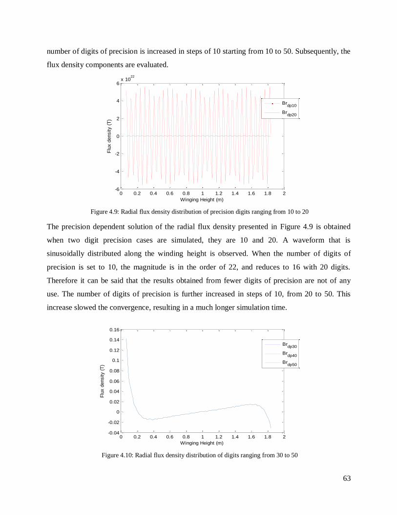
63
number of digits of precision is increased in steps of 10 starting from 10 to 50. Subsequently, the
flux density components are evaluated.
Figure 4.9: Radial flux density distribution of precision digits ranging from 10 to 20
The precision dependent solution of the radial flux density presented in Figure 4.9 is obtained
when two digit precision cases are simulated, they are 10 and 20. A waveform that is
sinusoidally distributed along the winding height is observed. When the number of digits of
precision is set to 10, the magnitude is in the order of 22, and reduces to 16 with 20 digits.
Therefore it can be said that the results obtained from fewer digits of precision are not of any
use. The number of digits of precision is further increased in steps of 10, from 20 to 50. This
increase slowed the convergence, resulting in a much longer simulation time.
Figure 4.10: Radial flux density distribution of digits ranging from 30 to 50
0 0.2 0.4 0.6 0.8 1 1.2 1.4 1.6 1.8 2-6
-4
-2
0
2
4
6x 10
22
Winging Height (m)
Flu
x d
ensity (
T)
Brdp10
Brdp20
0 0.2 0.4 0.6 0.8 1 1.2 1.4 1.6 1.8 2-0.04
-0.02
0
0.02
0.04
0.06
0.08
0.1
0.12
0.14
0.16
Winging Height (m)
Flu
x d
ensity (
T)
Brdp30
Brdp40
Brdp50

64
The increase of the number of digits of precision from 30 to 50 showed practical results. The
magnitude of the calculated flux density values reduced to more reliable results. It is noted that
there is no fundamental change of waveform shape as the precision is increased further. To
ensure that the obtained results are not coincidental, the axial flux density components are
studied separately below.
Figure 4.11: Axial flux density distribution of digits ranging from 10 to 20
Figure 4.12: Axial flux density distribution for precision digits ranging from 30 to 50
In Figure 4.11 and Figure 4.12, the number of digits of precision is changed in the same manner
as was done for the radial components. Varying the number of digits of precision from 10 to 50
yields the same behaviour. The important conclusion is however, that there is an exponential
0 0.2 0.4 0.6 0.8 1 1.2 1.4 1.6 1.8 2-6
-4
-2
0
2
4
6x 10
22
Winging Height (m)
Flu
x d
ensity (
T)
Bzdp10
Bzdp20
0 0.2 0.4 0.6 0.8 1 1.2 1.4 1.6 1.8 2-0.18
-0.17
-0.16
-0.15
-0.14
-0.13
-0.12
-0.11
-0.1
-0.09
-0.08
Winging Height (m)
Flu
x d
ensity (
T)
Bzdp30
Bzdp40
Bzdp50

65
relationship between accuracy and the number of digits of precision. This relationship can be
regarded as being directly proportional in the physical/ practical sense. This condition has shown
to be true for the number of digits of precision less than 30. In addition, the radial and axial flux
density components are exactly the same for the number of digit of precision larger than 30 as
seen in Figure 10 and Figure 4.12. This result emphasizes the need to ensure that the valid
number of digits of precision is known. The next subsection deals with the comparison of the
number of Fourier series terms against accuracy.
4.2.2. Number of series terms
It has been discussed how the number of digits of precision affects the magnitude of the flux
density values. Despite the previous assumption of regarding 70 elements as being sufficient, it is
important to understand the region of confidence when working with this number. It is known
that the number of elements of the series directly affects the computational speed. The advantage
of knowing the maximum number is that it accelerates the implementation.
In a mathematical sense, the optimal number of elements can be established using the derivative
of the function. If the subject of the field equation is n- terms and the derivative is equated to 0,
the maximum number is attainable. However, in view of the Fourier series equations being
mathematically abstract, the derivative route would introduce unnecessary difficulties. It is for
this very reason that the practical approach is adopted. In a similar setup to the examination of
number of digits of precision, the number of terms is studied. This number is increased from 10
to 70, and the radial and axial flux densities are recoded. A precision of 32-digits is used for all
the cases.

66
Figure 4. 13: Radial flux density distribution when the number of terms varies from 10 to 40
The above figure shows the result of having a 10 to 40 number of terms. The main reason the
results are presented in segments is the enhanced visualization. The numbers of terms drive the
harmonic distortion of the field distribution. When 10 elements are used the distortion is even
more visible.
Figure 4.14: Radial flux density distribution when the number of terms varies from 50 to 70
As soon as the terms reach 50 as shown in Figure 4.14 the ripple effect reduces rapidly. With 60
to 70 elements, it is seen that the results are completely settled. The use of 70 elements during
the assessment of number of digits of precision is therefore justified. To ensure that the number
0 0.2 0.4 0.6 0.8 1 1.2 1.4 1.6 1.8 2-0.06
-0.04
-0.02
0
0.02
0.04
0.06
0.08
0.1
0.12
0.14
Winding Height (m)
Flu
x d
ensity
Brn=10
Brn=20
Brn=30
Brn=40
0 0.2 0.4 0.6 0.8 1 1.2 1.4 1.6 1.8 2-0.04
-0.02
0
0.02
0.04
0.06
0.08
0.1
0.12
0.14
0.16
Winding Height (m)
Flu
x d
ensity
Brn=50
Brn=60
Brn=70

67
of the convergence seen is not component dependent, the axial flux density distribution is also
tested.
Figure 4.15: Axial flux density distribution when the number of terms varies from 10 to 40
The axial flux density distribution is similarly affected by the number of terms of the Fourier
series chosen. Although, the effect is less noticeable compared to the radial flux density
distribution. According to Figure 4.15, the harmonic distortion is less visible after 30 elements.
Figure 4.16: Axial flux density distribution when the number of terms varies from 50 to 70
In Figure 4.16, the analytical solution is already stable from 50 elements onwards. As the three
conditions are presented in a superimposed manner, it is not easy to distinguish between the three
0 0.2 0.4 0.6 0.8 1 1.2 1.4 1.6 1.8 2-0.18
-0.17
-0.16
-0.15
-0.14
-0.13
-0.12
-0.11
-0.1
-0.09
-0.08
Winding Height (m)
Flu
x d
ensity
Bzn=10
Bzn=20
Bzn=30
Bzn=40
0 0.2 0.4 0.6 0.8 1 1.2 1.4 1.6 1.8 2-0.18
-0.17
-0.16
-0.15
-0.14
-0.13
-0.12
-0.11
-0.1
-0.09
-0.08
Winding Height (m)
Flu
x d
ensity
Bzn=50
Bzn=60
Bzn=70

68
plots. The results match exactly from these three conditions. Through the detailed
implementation of Rabins’ method in Mathematica, the definite number of digits of precision
and the number of series terms are established. The 32-digits and 70 elements of the respective
parameters discussed above are further tested later in the discussion section. The next section
contains the use of the numerical method to determine field quantities.
4.3. Numerical approach
In the preceding section the analytical method has been implemented and the flux density
computed. The numerical results presented in this section are obtained from a simulation model
conducted in the commercial FEM software Ansoft Maxwell 14.0. In this program, the eddy
current simulation type is configured with the operating frequency of 50Hz. The geometry model
is similar to the one used in the previous section. The setup of this geometry is specified to be
axisymmetric. The geometric model parameters of this simulation and the loading data are
provided in Appendix B.
Figure 4.17: Maxwell simplified geometry model

69
In Figure 4.17, the transformer geometry is modelled; the 2-D cross-sectional view shows the
number of windings taken into account. The two windings are of different types. From the core
they are of helical and disc type respectively. The conductor types are continuously transposed
cable (CTC) and strip conductors for Winding A and B respectively.
During the simulation, the windings are geometrically constructed as solid blocks, albeit
configured to be stranded. This ensures that the eddy currents are not taken into consideration;
otherwise the model would require that the geometric detail be at the strand level. This modelling
approach is adequate since the attention is placed on evaluating the leakage field.
Given the number of discrete points of the field quantities required, a routine is developed. The
field quantities are therefore obtained from a parameterized model, one such is described in [8].
This automated process was written in Matlab. The centroid coordinates of all strand positions
are calculated from the knowledge of strand dimensions. The matrices containing flux density
components (r and z) in each strand position are extracted from the model. The flux density
components obtained from the above numerical method are then compared to the results
obtained using Rabins’ method. The accuracy is investigated with the change of winding height
to core window height ratio.
4.4. Results discussion
The analytical method has been implemented in Mathematica in Section 4.3. The number of
digits of precision and the number of the Fourier series terms have been investigated. The 32-
digits and 70 series terms proved to be sufficient for the computation. The simulation of the
implementation of the algorithms in Mathematica took approximately 15 minutes. To accelerate
the simulation time, parallel computing consisting of 16 kernels was configured.
In this section the analytical results are compared to those of FEM when computed at similar
positions. The FEM package utilized for the numerical results uses an adaptive solver. This
requires that the maximum number of convergence passes be set. Hence, the results compared
with analytical method were obtained after 14 passes. After each pass, the mesh elements are
increased by almost 30 per cent.

70
When implementing the numerical method under the stringent convergence criteria mentioned
above, the total simulation time was 32 seconds. This time can be broken down into
initialization, solving, and post-processing; with each process lasting 12, 16 and 4 seconds
respectively. The results obtained from both the analytical and numerical methods are shown
below; the axial and radial components are plotted in different figures.
Figure 4.18: Radial flux density from FEM and Rabins’ method
In Figure 4.18, the radial flux density components evaluated using FEM and Rabins’ methods are
shown. The flux density values of winding A are plotted across the winding height with 132
discrete points. It is clear from the diagram that the fundamental distribution of the field for both
methods is periodic with similar profiles. However, the magnitude differs. The maximum for
FEM is 0.1 T, while Rabins yields 0.14 T. This difference is large and may result in the
overestimation of the winding hot-spot factors when losses are calculated.
0 0.2 0.4 0.6 0.8 1 1.2 1.4 1.6 1.8 2-0.2
-0.15
-0.1
-0.05
0
0.05
0.1
0.15
Winding Height (m)
Flu
x d
ensity (
T)
BrFEM
BrRab
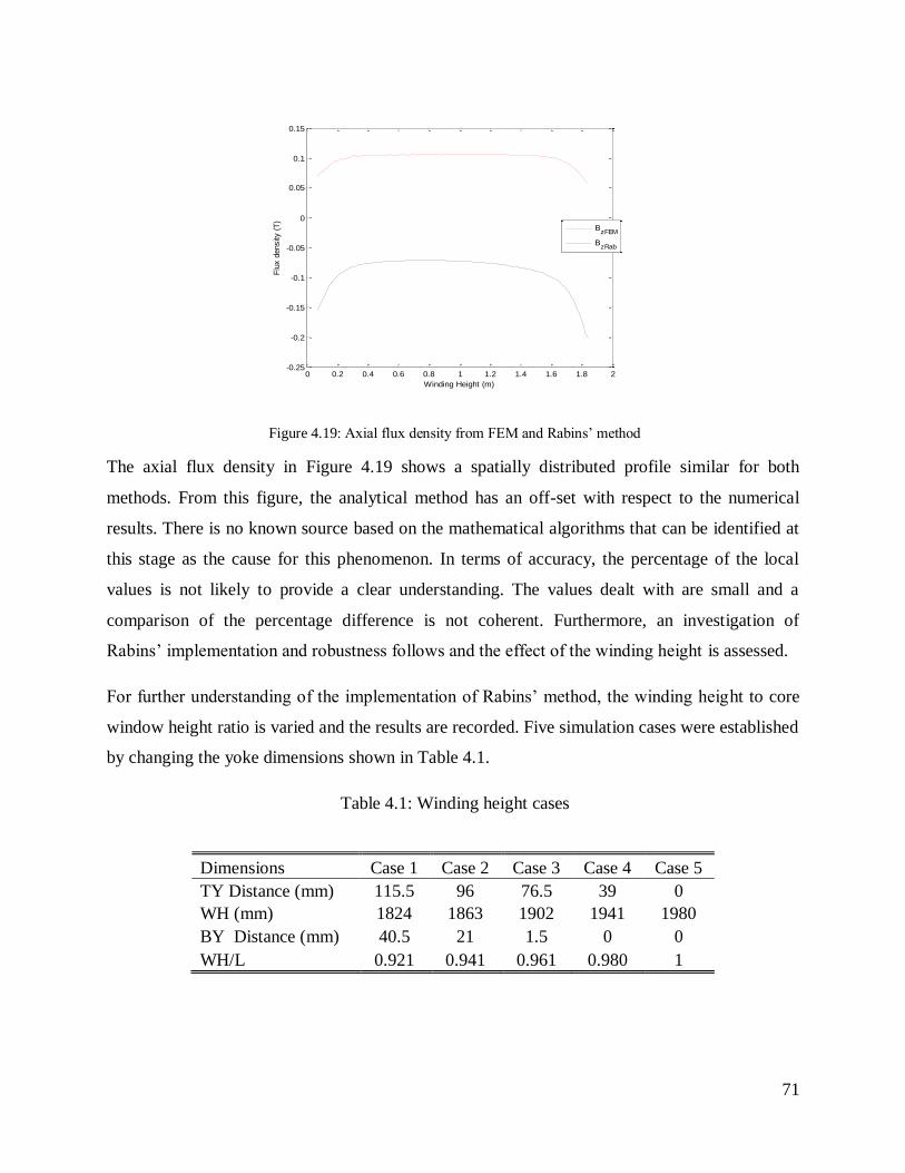
71
Figure 4.19: Axial flux density from FEM and Rabins’ method
The axial flux density in Figure 4.19 shows a spatially distributed profile similar for both
methods. From this figure, the analytical method has an off-set with respect to the numerical
results. There is no known source based on the mathematical algorithms that can be identified at
this stage as the cause for this phenomenon. In terms of accuracy, the percentage of the local
values is not likely to provide a clear understanding. The values dealt with are small and a
comparison of the percentage difference is not coherent. Furthermore, an investigation of
Rabins’ implementation and robustness follows and the effect of the winding height is assessed.
For further understanding of the implementation of Rabins’ method, the winding height to core
window height ratio is varied and the results are recorded. Five simulation cases were established
by changing the yoke dimensions shown in Table 4.1.
Table 4.1: Winding height cases
Dimensions Case 1 Case 2 Case 3 Case 4 Case 5
TY Distance (mm) 115.5 96 76.5 39 0
WH (mm) 1824 1863 1902 1941 1980
BY Distance (mm) 40.5 21 1.5 0 0
WH/L 0.921 0.941 0.961 0.980 1
0 0.2 0.4 0.6 0.8 1 1.2 1.4 1.6 1.8 2-0.25
-0.2
-0.15
-0.1
-0.05
0
0.05
0.1
0.15
Winding Height (m)
Flu
x d
ensity (
T)
BzFEM
BzRab

72
The simulation cases presented in Table 4.1 were simulated in FEM and Mathematica. For the
first four cases, only one case is reported which is Case 2. This is because the computational
aspect did not change significantly. The results of Case 5 became interesting as the mathematical
expectation differs from the numerical solution. As the field quantities are determined, the
simulation time of 70 elements took approximately 25 minutes for each case. The field quantities
of Case 2 and Case 5 are presented on the graphs below.
Figure 4.20: Radial flux density distribution of Case 2
The sluggish convergence experienced is attributed to insufficient number of digits of precision
used. Therefore the earlier assumption of 32-digits being adequate does not hold for all cases.
The results of the simulation returned a matrix with a mix of high exponent values. These were
discarded to make a comparison of only valid data due to numerical instability of Rabins’
method. This is evident in Figure 4.20; the discontinuities seen are due to the removal of invalid
data. However it is observed that the fundamental shape of the distribution is sustained.
-0.15
-0.10
-0.05
0.00
0.05
0.10
0.000 0.500 1.000 1.500 2.000
Flu
x d
ensi
ty (
T)
Winding Height (m)
FEM
Rab

73
Figure 4.21: Axial flux density distribution of Case 2
The axial flux density results of Case 2 in Figure 4.21 are no different to the radial field
distribution in terms of discontinuities. It is observed that the off-set of the magnitude persists.
But, in pursuit of understanding the cause, the Case 5 results are expected to share important
insight.
Figure 4.22: Radial flux density distribution of Case 5
The special case amongst all the cases is Case 5. The winding height is equal to the core window
height. Mathematically, the periodicity falls away as the current distribution is governed by the
dc term. This leaves only the axial component of the field.
-0.25
-0.20
-0.15
-0.10
-0.05
0.00
0.05
0.10
0.15
0.000 0.500 1.000 1.500 2.000F
lux d
ensi
ty (
T)
Winding Height (m)
FEM
Rab
0 0.2 0.4 0.6 0.8 1 1.2 1.4 1.6 1.8 2-0.03
-0.02
-0.01
0
0.01
0.02
0.03
0.04
0.05
0.06
0.07
Winding Height (m)
Flu
x d
ensity (
T)
BrFEM
BrRab

74
The analytical solution in Figure 4.22 shows that the aforementioned mathematical behaviour is
achieved. The radial flux density is flat at 0 T along the winding height. However, the numerical
method result shows that the radial flux density does not become 0 T. The maximum flux density
obtained is 0.06 T. The difference of these results to the ones previously achieved is the positions
of the maxima along the height. Traditionally, the maximum radial fields are obtained towards
the winding ends, which is not the case here. It is therefore proposed that the main cause of the
effect is the adjacent winding. Since the analytical solution does not take into account the
geometric influence of the adjacent winding, it is not easy to capture this profile analytically.
Figure 4.23: Axial flux density distribution of Case 5
From Figure 4.23 above, the axial flux density is constant at -0.114 T. This satisfies the
orthogonality of the field on the boundaries of the yokes. The same cannot be said from the FEM
results as the field is not constant along the height. The explanation of this cause has been
provided above on the radial flux density account. Moreover, the magnitude difference between
the numerical and analytical results is of concern. The definition of the current direction may be
the cause; in the implementation of the analytical method, the current of the winding has a
negative polarity. Figure 4.24 depicts the flux density with the results of the predicted off-set of
0.2 T.
0 0.2 0.4 0.6 0.8 1 1.2 1.4 1.6 1.8 2-0.15
-0.1
-0.05
0
0.05
0.1
0.15
Winding Height (m)
Flu
x d
ensity (
T)
BzFEM
BzRab

75
Figure 4.24: Assessment of the off-set for axial flux density distribution
The axial flux density distribution of the results presented so far shows a consistent off-set, even
the simple dc case shown in Figure 4.23. It is therefore important to understand the origin of this
off-set. Through a random search of possible dc off-set from the multitude of results shown in
this section a value of 0.2 T is established. Furthermore, the results shown earlier in Figure 4.19
are used to examine the accuracy of the off-set illustrated in Figure 4.24. From these results, the
minimum error achieved with the off-set of 0.2 T is 0.32%, while maximum is 10.905 %.
From the set of results presented, the exact number of digit of precision is not known; however it
is proven that it should be more than 32-digits of precision. Also it has been shown that this
number can be influenced by the geometric dimension, such as the variation of the limb height
that was assessed. This makes it difficult to define the exact number of digits of precision that
satisfies a large range.
4.5. Conclusion
The implementation of the leakage field computational methods showed that the numerical
method is accurate, flexible and fast. This makes the numerical method a preferred method that
transformer designers should rely on for calculating leakage fields.
For the analytical method, the number of Fourier series terms should at least exceed 50 to obtain
meaningful results. In addition, more than 32-digits of precision are required to successfully
implement Rabins’ method. The stability of the analytical method is dependent on the
0 0.2 0.4 0.6 0.8 1 1.2 1.4 1.6 1.8 20.02
0.03
0.04
0.05
0.06
0.07
0.08
0.09
0.1
0.11
0.12
Winding Height (m)
Flux
den
sity
(T)
Bz (actual)
Boff-set

76
transformer geometry, with the winding height to core window height ratio influencing the
results significantly.
Lastly, the leakage flux patterns obtained using Rabins’ method and FEM compared well, thus
justifying the relevance of Rabins’ method in the modern environment. Although, it is seen that
the implementation of Rabins’ method is tough and mathematically abstract, lower level
programming platforms can be used to improve the speed. Rabins’ method results are used to
compare the winding eddy losses in Chapters 5 and 6 to validate the 2-D FEM results.

77
Chapter 5
Core window effect on the calculation of winding eddy losses
In the previous chapter, different aspects of the computation of the leakage field quantities that
are significant to the calculation of winding eddy losses are presented. It is clear that the
numerical model approach is robust, flexible and fast for two-dimensional transformer models.
The common practice in modelling transformers for loss calculations in transformer windings
involves two-dimensional methods which are implicitly accepted as accurate [54]. However, the
two-dimensional modelling approach of a transformer does not entirely represent the field
distributions in all areas of the transformer winding. This chapter assesses the distribution of the
flux density components around the winding circumference. It further quantifies the effect of this
distribution to the winding eddy losses.
In most practical designs, sections of the winding conductors are situated on the inside and the
others on the outside of the core window. The situation is such that the windings are subject to
different leakage field levels. In this chapter, this phenomenon will be referred to as the “core
window effect”. The only methodologies able to account for this effect should have capacity to
model the complete three-dimensional structure of the transformer.
The methods presented so far for calculating winding eddy losses are inherently applicable to the

78
2-D axisymmetric model, involuntarily neglecting the core window effect. As indicated earlier,
this is because most transformer manufacturers find it easy to embed this calculation
methodology in their design routine programs. Most solvers of these programs are configured to
conduct simulation in the axisymmetric and planar domains. Kulkarni et al [8] developed such a
routine; although there are other handfuls of such unpublished programs. Moreover, there is an
abundance of 2-D FEM packages that are freely or commercially available.
Several authors have used three-dimensional methods to determine winding eddy losses. For an
instance, Saley et al [7] developed a 3-D program to calculate the three-dimensional field using
the integral equation techniques. Also, Girgis et al [55] performed field measurements in the
windings of a shell-form transformer. Their aim was to verify the three-dimensional tool they
had developed earlier [56]. What is common amongst these attempts is the failure to comment on
field distribution around the circumference of the winding.
Waters [57] conducted a practical experiment to evaluate the radial field for the calculation of
axial forces. He commented that the radial field inside the window is 20 to 50 % greater than the
mean value. However, his comments are limited only to the measured radial field components. In
addition, there is no other known published work on the critical analysis of the core window
effect.
The purpose of this chapter is to analyse the field distribution along the circumference of the
transformer winding, further examining the overall effect of the core window to the winding
eddy loss evaluation. Subsequently, the core window effect is evaluated through field quantities
determined from three-dimensional models of different simulation types such as:
Magnetostatic
Transient
Eddy current
The availability of the full version of Ansoft Maxwell 14.0 comes in handy when performing
analyses of this nature. A core-type, three phase, three winding transformer is simulated in this
FEM package and the results are presented. This model is used to assess the contribution of the
winding to core distance and also the effect of the adjacent windings.
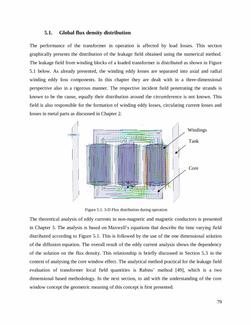
79
5.1. Global flux density distribution
The performance of the transformer in operation is affected by load losses. This section
graphically presents the distribution of the leakage field obtained using the numerical method.
The leakage field from winding blocks of a loaded transformer is distributed as shown in Figure
5.1 below. As already presented, the winding eddy losses are separated into axial and radial
winding eddy loss components. In this chapter they are dealt with in a three-dimensional
perspective also in a rigorous manner. The respective incident field penetrating the strands is
known to be the cause, equally their distribution around the circumference is not known. This
field is also responsible for the formation of winding eddy losses, circulating current losses and
losses in metal parts as discussed in Chapter 2.
Figure 5.1: 3-D Flux distribution during operation
The theoretical analysis of eddy currents in non-magnetic and magnetic conductors is presented
in Chapter 3. The analysis is based on Maxwell’s equations that describe the time varying field
distributed according to Figure 5.1. This is followed by the use of the one dimensional solution
of the diffusion equation. The overall result of the eddy current analysis shows the dependency
of the solution on the flux density. This relationship is briefly discussed in Section 5.3 in the
context of analysing the core window effect. The analytical method practical for the leakage field
evaluation of transformer local field quantities is Rabins’ method [49], which is a two
dimensional based methodology. In the next section, to aid with the understanding of the core
window concept the geometric meaning of this concept is first presented.
Windings
Tank
Core
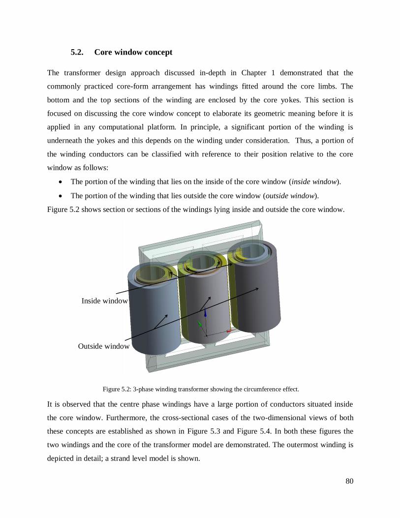
80
5.2. Core window concept
The transformer design approach discussed in-depth in Chapter 1 demonstrated that the
commonly practiced core-form arrangement has windings fitted around the core limbs. The
bottom and the top sections of the winding are enclosed by the core yokes. This section is
focused on discussing the core window concept to elaborate its geometric meaning before it is
applied in any computational platform. In principle, a significant portion of the winding is
underneath the yokes and this depends on the winding under consideration. Thus, a portion of
the winding conductors can be classified with reference to their position relative to the core
window as follows:
The portion of the winding that lies on the inside of the core window (inside window).
The portion of the winding that lies outside the core window (outside window).
Figure 5.2 shows section or sections of the windings lying inside and outside the core window.
Figure 5.2: 3-phase winding transformer showing the circumference effect.
It is observed that the centre phase windings have a large portion of conductors situated inside
the core window. Furthermore, the cross-sectional cases of the two-dimensional views of both
these concepts are established as shown in Figure 5.3 and Figure 5.4. In both these figures the
two windings and the core of the transformer model are demonstrated. The outermost winding is
depicted in detail; a strand level model is shown.
Inside window
Outside window

81
Figure 5.3: Winding sections situated inside the core window
Figure 5.4: Outside core window winding sections
Across the 360° circumference, a winding is likely to be covered by the yokes as seen in Figure
5.2, and it can be approximated that a quarter to a third of the winding conductors lie inside the
core window. It is known that the leakage field inside the core window is different to that outside
the core window; the next sections will discuss the quantity of this difference. Typically, the
field penetrates the yoke at a right angle, which is why the solution of the field in [49] permits
the assumption of infinite permeability of the yokes. At this stage, the difference between the

82
field inside the core window and outside of the core window has not been well established.
The presence of the core over certain sections of the winding conductors influences the
reluctance path across the circumference. Thus, the reluctance paths travelled by the field in the
outer and inner core window regions require a meticulous computation of the field around the
circumference to clearly understand this effect.
5.3. Calculation of winding eddy losses
The winding conductors are subject to two components of the incident field, namely the axial
and radial flux density components. The consequence of this field penetrating the strands is the
winding eddy losses. The detailed formulation resulting in the governing equation outlined in
Equation 5.1 is covered thoroughly in Chapter 3. In this section the importance of understanding
the leakage field distribution to evaluate the losses is emphasized. The result of the analytical
equation is the loss density in Watts per cubic meters of each strand as follows:
(5.1)
The next step is to obtain the losses in Watts, done by multiplying the loss density by the strand
volume. Additionally, it is seen later in the discussion section that this can also be achieved by
integrating the flux density over the volume domain. Below, Equations 5.2 and 5.3 define the
loss components as a function of the number of strands for both the radial and axial components.
These representations show the computation of winding eddy losses using the field quantities
obtained at the mid-point of each strand.
∑ ∑ ( )
(5.2)
∑ ∑
(5.3)
From (5.2) and (5.3), it is obvious that the losses are proportional to the square of the flux
density components. This relationship is important to conductors situated in the same radial
position along the winding height. These strands will have the same volume throughout the

83
winding height provided their dimensions are the same. In addition, most practical applications
use the same winding strand dimensions per winding.
(5.4)
(5.5)
According to Equations 5.4 and 5.5, for the better estimation of losses, the local flux density
components require a high degree of accuracy during computations. This underpins the need for
a rigorous investigation of the core window effect. The analysis of the core window effect avails
the flux density components in differential volumes around the circumference.
5.4. Transformer modelling using 3-D FEM
The previous sections have laid the ground work involving the description of the core window
effect. Section 5.3 provided insight on how the flux density distribution around the winding
circumference affects the winding eddy losses. The transformer model used for the analysis of
the three-dimensional leakage field is presented in this section. The size of the transformer is
40MVA, and the transformer is double-wound. The selection of this unit is motivated by the
large number of batches that have been manufactured and tested at Powertech Transformers’
Pretoria West plant. The measured load losses of eleven units of this design will be presented in
the next chapter.
The transformer under consideration has three windings in each limb, the detailed winding
design of each is provided in Appendix C. The geometry is set up in the FEM simulation
package ANSYS module “Design Modeler” and exported to Ansoft Maxwell for the calculation
of field quantities. The advantage of this approach is the flexibility of the ANSYS package in
interweaving the multidisciplinary modules. There are two transformer models established
explicitly for the analysis of the core window effect. The first is the single phase case, it is used
to analyse the distance to core yoke effect. Meanwhile, the three phase case is used to provide
the understanding of the leakage field distribution in each phase and how these are affected by
the adjacent windings. Finally, the eddy current simulation is prepared for computing the
winding eddy losses.

84
Figure 5.5 a: Single-phase configuration Figure 5.5 b: Three-phase configuration
Once the model is exported to Maxwell, the transformer excitation, loading parameters and
boundary conditions are assigned. The excitation data for this specific transformer is provided in
Table 5.1.
Table 5.1: 40 MVA excitation data
Winding A Winding B Winding C
Turns 163 56 1072
Current (A) 1210.7 174.95 174.95
Winding type Helical Loop layer Disc
Maxwell uses the adaptive technique to find the converging simulation results. As such, the input
parameters of the convergence criterion include the setting of percentage energy error and mesh
refinement. However, to improve accuracy, advanced meshing principles can be applied to
optimize the simulation time. As an example, seven passes were selected for the eddy current
simulation, and the advanced mesh techniques were configured to improve the simulation time.
The convergence behaviour obtained as the change of the energy percentage error is depicted in
Figure 5.6. The energy error criterion was set at 0.1% of each iterative pass.
Core
Windings Windings
Core
A A B B C C
C B A C B A C B A C B A

85
Figure 5.6 : Energy error changes per adaptive pass
From Figure 5.6, the energy error decays exponentially as the number of passes increases. This
indicates the sufficiency of the choice of seven iterative passes as where the global energy error
decays below 0.1%. The results obtained after the convergence of the solution are post-processed
in the next sections. The magnetostatic, eddy current and transient solutions are presented for the
purposes already mentioned.
5.5. Results post-processing procedure
Immediately after the simulation run is completed, the field quantities became available from the
components defined by the transformer geometry model. This section describes how the field
quantities are obtained from the model. In addition, the focus is placed only on the regions
applicable to the window sections. These are of utmost importance for the study of the core
window effect. Two methods are used to extract the field quantities namely; through a non-
model object line or using coordinates text file as an input. Both methods are explained briefly in
this section.
These two methods are applied intensively to post-process the field distribution. A non-model
circular polyline is drawn around one winding object of the simulated transformer model. This
line can be duplicated to the remaining phases of interest, especially in the three- phase
1 2 3 4 5 6 70
0.5
1
1.5
Number of adaptive passes
Ene
rgy
erro
r (%
)

86
simulation model. Here, the z coordinate of the lines is the top of winding A (1682 mm) as
provided in Appendix C, and this location is used throughout the analysis. The choice of this
location is already observed in the preceding chapter where; it was shown that the radial flux
density becomes significantly higher towards the winding ends. Figure 5.7 illustrates this line
drawn in each winding for the acquisition of field quantities.
Figure 5.7: Non-model object line drawn for the acquisition of the flux density
The alternative to the method presented above is to obtain field quantities in the circumferential
direction by extracting them using an automated routine. Such a routine is written in Matlab to
transform the Polar coordinates data to Cartesian coordinates. The x and y coordinates are
calculated with a 0.36° step change equivalent to Polar coordinates. This yields 1001 sample
points around the circumference. The corresponding flux density components are then extracted
from the model.
For the analysis of the flux density, the “field calculator” in Maxwell is used. Both methods of
attaining flux density components are used with the calculator. However, for simplicity, the first
method is preferred. This is because it is more robust and achievable with few computational
steps. The second method is also used in circumstances where the drawing of the non-model
object is considered challenging.
Measurement line
A
B
C

87
For the study of the circumference flux density distribution, the field quantities are plotted on the
polar coordinates system. The selection of this approach is mainly to enhance the visualization of
the distribution of the field components. Following this discussion, the next sections present the
results obtained using either one of the above methods.
5.6. Circumferential field distribution
The sets of results reported in this section are primarily the flux density components obtained
around the circumference of winding A from a magnetostatic simulation. The flux density values
of interest are those calculated at the mid radial dimension of the winding. The results are post-
processed in the manner described in the previous section.
The full ampere-turns are assigned to phase A, meanwhile phases B and C have the same half
ampere-turns in the opposite direction. This is to ensure that there is an ampere-turn balance, i.e.
the sum of all winding ampere-turn values is approximately equal to zero. With the use of the
field calculator in Maxwell as earlier reported, the field equations for the r and z components of
the flux density are defined. It is already mentioned that the results are acquired at 0.36°
resolution. This resolution is considered sufficient to observe the changes of the flux density
components. This is evident in the graphical results presented in this section.
The results of the setup described above are presented in Figures 5.8 and 5.9 for radial and axial
components of the flux density respectively. The two components are assessed individually
below.

88
Figure 5.8: Radial flux density distribution around the circumference
Figure 5.8 shows the radial flux distribution for phase A, B and C around the circumference. It is
noted that the magnitude of phase A is higher than B and C which is expected. This is due to the
proportional relationship between the current and the flux density. Furthermore, the radial flux
component plotted above is the magnitude of the x and y components. This is in part due to the
coordinate system transformation of Bx and By to cylindrical coordinate system components r and
z. Hence, the radial field is analysed using the magnitude only.
The maximum flux density of phase A is approximately 0.08 T; meanwhile the minimum is 0.06
T. This difference between the two extreme values yields 25%. The flux density of the other two
phases is distributed in a similar manner to that of phase A; the exception is phase B. In this
phase the distribution shrinks inwards on the right hand side of Figure 5.8. The flux density
distributions of the three phases clearly indicate that there is a reduction of the radial components
on the sections covered by the core. The next figure shows the distribution of the axial field in
the same locations. This plot serves to provide insight on how axial field levels of the sections
under the core window are affected.
0.02
0.04
0.06
0.08
30
210
60
240
90
270
120
300
150
330
180 0
Br
p A Br
p B Br
p C
Circumference (°)
Flu
x d
ensi
ty (
T)

89
Figure 5.9: Axial flux distribution for phase A, B and C along the circumference
Similarly with the assessment of the radial component, the results of axial flux density are
acquired and shown in Figure 5.9. However, the axial component does not need an additional
manipulation as the z component is the same for both the cylindrical and rectangular coordinate
systems. Phase A has the magnitude of approximately 0.036 T. The peak is observed on the path
of 270° to 90°, strictly in the anticlockwise direction. The difference between the maximum and
the minimum field is approximately 16% of the maximum flux density of 0.041T. Essentially,
the axial flux density distribution is almost uniform across the circumference of the winding.
This immediately implies that the radial field components are more significantly affected by the
core window as compared to the axial component.
The distribution of phase B and C is equal in magnitude across the circumference of the
windings. Notably, the two components show the peak in the same direction as illustrated in
Figure 5.9. The latter confirms that apart from the presence of the core, the adjacent windings
cause the non-uniform distribution of the field. Lastly, at this stage it is not clear whether the
non-uniform distribution is due to the presence of the core or the ampere-turn of the adjacent
windings. To further understand the core window phenomenon, the change of the winding to
0.01
0.02
0.03
0.04
0.05
30
210
60
240
90
270
120
300
150
330
180 0
Bz
p A Bz
p B Bz
p C
Circumference (°)
Flu
x d
ensi
ty (
T)

90
core yoke distance is studied. In addition, the effect of the adjacent winding is assessed using the
transient simulation. It is also established later how the field quantities deviate from the average.
5.7. Effect of the winding to core yoke distance
In the preceding section it is mentioned that there is no obvious evidence of the main cause of the
non-uniform behaviour of the field around the circumference of the winding. Consequently, an
additional simulation of the single phase model was setup. This simulation is a single phase
transformer of three limbs. Since the aim is only to assess the core window effect the same unit
was selected with few alterations. In this model the windings of the side limbs are removed.
The assessment of the core window is conducted through a simulation of numerous design points
that are established. In each design point the limb height of 1808 mm as shown in Appendix C is
reduced by 21 mm. However, the minimum case is the limb height of 1684 mm as shown in
Table 5.2. According to the 21 mm reduction this value should be 1682, however, to prevent a
convergence problem a 2 mm gap is reserved. Table 5.2 shows all simulation cases considered
for the analysis of the winding to core yoke distance effect.
Table 5.2: Single phase parametric design points
Simulation
Case
Limb
Height (mm)
Winding to Top
Yoke (mm)
1 1808 126
2 1787 105
3 1766 84
4 1745 63
5 1724 42
6 1703 21
7 1684 2
To prepare these design cases, the geometry model of the test transformer is parameterized in the
ANSYS module, Design Modeler. This environment is flexible to small changes of the geometry
and application of the optimization tools as earlier indicated. Essentially, the seven design

91
models presented in Table 5.2 should be individually prepared by manually changing the
parametric values. However, in ANSYS workbench there is a variety of design optimization
tools which are tailored to the parametric modelling approach. As a result one of these tools
called “Response Surface” was manipulated to instantly create seven design points. In addition,
for the full use of this tool an independent “DesignXplore” component “Optometrics” in
Maxwell is required. Due to a lack of this resource the full simulation of each model is not
automatically accomplished. These simulation models are updated manually.
Through the development of the numerous models of different limb height dimensions, the
results of flux densities are extracted and presented. The results of the flux density distribution
around the circumference of the winding for the single phase transformer are shown in Figure
5.10 and Figure 5.11.
Figure 5.10: Radial flux distribution across the winding circumference
It is shown in Figure 5.10 that the radial flux density is proportional to the winding to core yoke
distance. For the winding to core yoke distance of 2 mm the radial flux density approaches zero
inside the core window. The distribution of the radial component is symmetric both in the x and y
planes, hence the core window effect accounts for 22°out of the 90°. This is the angle at which
0.02
0.04
0.06
0.08
30
210
60
240
90
270
120
300
150
330
180 0
Br1682 Br1702 Br1724
Br1766 Br1787 Br1808
Br1745
Circumference (°)
Flu
x d
ensi
ty (
T)

92
the field is visibly deviating from the circular line or the mean value. It is also observed that the
high winding to core yoke distance is indispensable to achieve a uniform distribution of the
radial flux density components. Furthermore, the minimum flux density of 0.00298T is observed
when the minimum winding to core yoke distance is 2 mm. This flux density value is 95.25 %
lower than the maximum.
For the same geometry configuration the distribution of axial flux density components was also
analysed. Flux density attained by varying the geometry according to Table 5.2 is shown in
Figure 5.11.
Figure 5.11: Axial flux distribution across the winding circumference
The results of the axial flux density of different winding to core yoke distances are shown in
Figure 5.11, it is apparent that the axial field component is inversely proportional to this distance.
This is also followed by the irregular distribution of the field around the winding circumference.
At the extreme minimum distance of 2 mm the orientation indicates the maximum flux density to
be inside the core window. It is also evident that the field distribution is almost symmetrical in
the x and y plane. Effectively, out of 90° the core window effect accounts for 30°. However, the
0.05
0.1
0.15
30
210
60
240
90
270
120
300
150
330
180 0
Bz1787 Bz1766 Bz1745
Bz1702
Bz1808
Circumference (°)
Flu
x d
ensi
ty (
T)
Bz1724
Bz1682

93
higher winding to core yoke distances illustrate that the non-uniform distribution of the field
diminishes. The latter is seen when the limb height is 1808 mm.
To understand the real meaning of the results, it is necessary to compare the mean flux density
against the actual flux density distribution. Thus, the leakage field distribution of the minimum
case is compared against the average.
Figure 5.12: Radial flux density plotted with the average value
Figure 5.12 shows the radial flux density obtained when the limb height is 1684 mm. The mean
flux density distribution around the circumference is 0.0532 T. It is assumed that this line
represents the 2-D axisymmetric case. The actual radial distribution around the circumference
fails to track the mean value. This is an indication that at low winding to core yoke distances, the
consequences of the core window effect could be significant. For practical applications, the
aforementioned distance is not common. Distances larger than 100 mm at the top and 60mm at
the bottom are ordinarily used. These distances are dictated by dielectric clearance requirements
and pressing of the top and bottom winding ends.
It is also observed from Figure 5.12 that the task of assessing the core window effect is complex
when using two dimensional tools. There are two main prevailing behaviours observed:
0.02
0.04
0.06
0.08
30
210
60
240
90
270
120
300
150
330
180 0
Br1682 Brav168
2
Flu
x d
ensi
ty (
T)
Circumference (°)

94
The radial flux component outside the core window section is larger than the mean value.
The section of the winding circumference lying inside the core window is subject to
lower field values than the mean.
To further analyse this phenomenon, the axial field is studied against the mean.
Figure 5.13: Radial flux density plotted with the average value
Illustrated in Figure 5.13 is the average distribution of the axial flux density across the winding
circumference, which is shown as a red dotted plot. It is the mean value calculated by taking all
axial flux densities across 360°. The critical observation from this distribution is the intersection
points of the actual and average distribution located at 30°, 150°, 210° and 330°. The average
flux density is 0.05168 T, the maximum flux density deviates by approximately 128.3%. It
should also be mentioned that this point is a peak value and may have little consequence on the
overall losses.
The result of the study of the effect of the core window effect has so far shown that the sections
under the core window will experience high axial field and low radial field intensities. The
findings are congruent with the conclusion made during the implementation of Rabins’ method
[49] in Chapter 4 where, the boundary conditions at the yokes incorporate the assumption that
0.05
0.1
0.15
30
210
60
240
90
270
120
300
150
330
180 0
Bz1682 Bzav1682
Flu
x d
ensi
ty (
T)
Circumference (°)

95
the field is normal to the yokes. In addition, the results of the study presented in this chapter are
found to oppose the conclusions drawn by Waters [57]. In his studies of the axial forces he
comments that the presence of the core does not cause the concentration of flux around the
circumference. The polar plot presented in his paper show uniformly distributed radial flux
density. Therefore, according to the study in this section the core has an effect dependant on the
distance between the winding and the core yokes. A great deal of details will be missed if the
variation of this distance is not done.
5.8. Transient analysis
The analyses of the flux density distribution discussed in Section 5.6 show that the adjacent
windings influence the field around the circumference. In order to establish the extent of this
influence, a transient simulation is required. In this section the study of flux density distribution
around the circumference during different time intervals of the sinusoidal excitation is
undertaken. From the knowledge of the period of the full 50 Hz sinusoidal signal, six simulation
points were considered. The simulation runs from a time step of 0s to 0.02s, in steps of 0.004s.
The transient discrete simulation points are depicted in Figure 5.14.
Figure 5.14: Sinusoidal excitation with discrete transient simulation points
In Figure 5.14, the ampere-turns of each phase are shown in the sinusoidal form. The ampere-turn
unbalance of the simulation points was also calculated discretely to confirm that it approached
zero.
0 0.002 0.004 0.006 0.008 0.01 0.012 0.014 0.016 0.018 0.02-2
-1.5
-1
-0.5
0
0.5
1
1.5
2x 10
5
Time (s)
Am
pere
turn
(A
t)
phaseA
phaseB
phaseC

96
The three-dimensional model already prepared during magnetostatic simulation is reconfigured
for the transient analysis. The results obtained for the first windings of each phase are presented
for t=0, 0.004 and 0.012 s. In each of the above mentioned points the winding A magnitude
contours of the field is plotted. Figure (a) of 5.15 to 5.17 is the radial flux density component.
Similarly, Figure (b) is the axial flux density component.
Figure 5.15a: Radial flux density at t=0 Figure 5.15 b: Axial flux density at t=0
Figure 5.16a: Radial flux density at t=0.004 Figure 5.16 b: Axial flux density at t=0.004
Phase A Phase B Phase C Phase A Phase B Phase C
Phase A Phase B Phase C Phase A Phase B Phase C
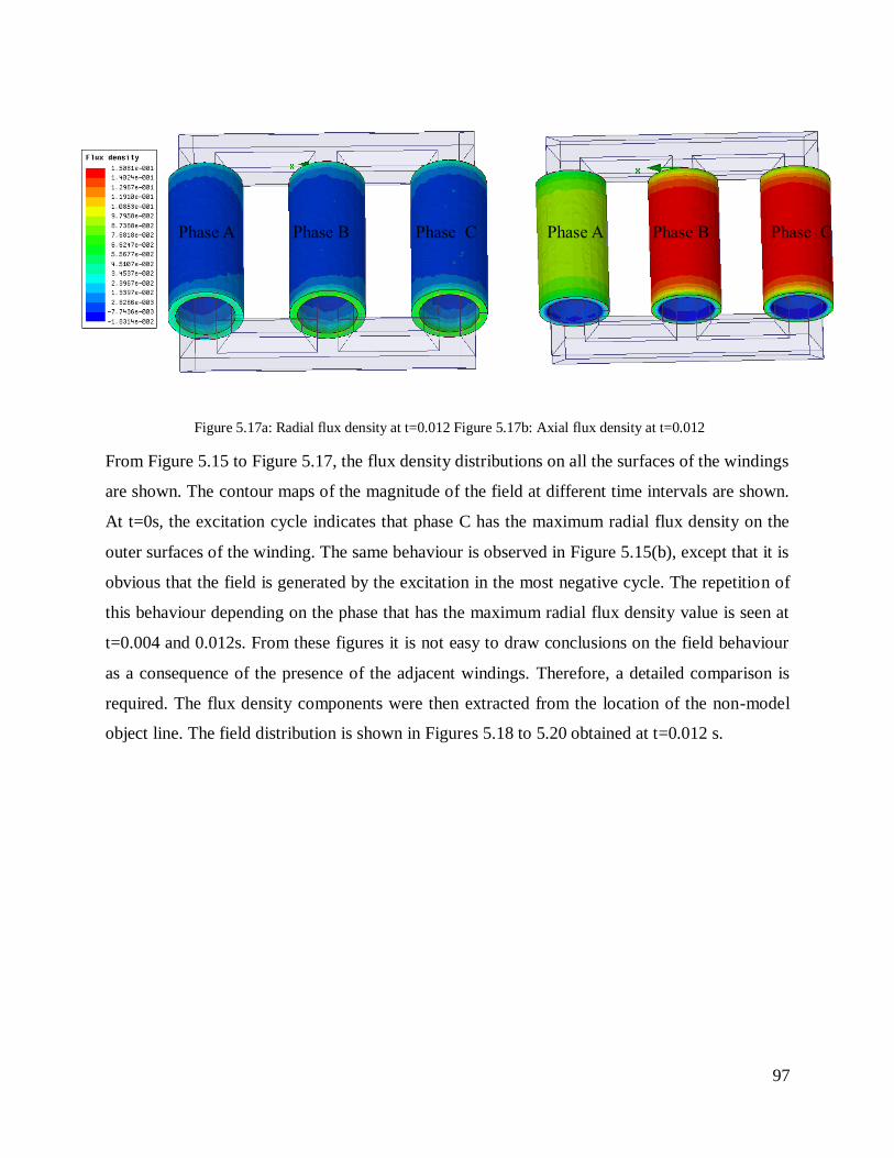
97
Figure 5.17a: Radial flux density at t=0.012 Figure 5.17b: Axial flux density at t=0.012
From Figure 5.15 to Figure 5.17, the flux density distributions on all the surfaces of the windings
are shown. The contour maps of the magnitude of the field at different time intervals are shown.
At t=0s, the excitation cycle indicates that phase C has the maximum radial flux density on the
outer surfaces of the winding. The same behaviour is observed in Figure 5.15(b), except that it is
obvious that the field is generated by the excitation in the most negative cycle. The repetition of
this behaviour depending on the phase that has the maximum radial flux density value is seen at
t=0.004 and 0.012s. From these figures it is not easy to draw conclusions on the field behaviour
as a consequence of the presence of the adjacent windings. Therefore, a detailed comparison is
required. The flux density components were then extracted from the location of the non-model
object line. The field distribution is shown in Figures 5.18 to 5.20 obtained at t=0.012 s.
Phase A Phase B Phase C Phase A Phase B Phase C

98
Figure 5.18: Flux density distribution of phase A at t =0.012 s
The results shown in Figure 5.18 have ripples; up to so far smooth results have been obtained.
These ripples are an indication that the mesh elements regarded sufficient for a magnetostatic
solution may be inadequate for the transient analysis. Nonetheless a conclusion is drawn from
these results since the fundamental profile is preserved. There is an evident shift of both flux
density component quantities showing an increase from the 90° to 270° quadrants.
0.02
0.04
0.06
0.08
30
210
60
240
90
270
120
300
150
330
180 0
Br p A
Bz p A
Flu
x d
ensi
ty (
T)
Circumference (°)

99
Figure 5.19: Flux density distribution of phase B at t =0.012 s
Figure 5.19 shows the radial and axial flux density components of phase B at t=0.012s. There is
a shift of the maximum radial flux density distribution leaning towards the 90° to 270°
quadrants. The peak of the axial flux density component is shifted along the path of 270° to 90°
quadrants. The characteristics of the field distribution of a single phase in a 3 limb transformer
have already been established from the previous section. The results of this phase are supposedly
equivalent to the single phase transformer case if the effect of the adjacent winding is neglected.
Therefore, this can assist in distinguishing the contribution of the adjacent windings.
The axial flux density of phase B is almost half that of phase A at approximately 0.02 T. The
same can be said for the radial component which is estimated at 0.04 T in comparison to 0.08T in
Figure 5.18. The field distribution is almost symmetric only in the x plane.
The axial and radial flux densities of the single phase illustrated symmetry in the x and y planes
of the distribution of flux densities around the circumference. The fact that the field distribution
observed on this phase in Figure 5.19 is shifted towards the opposite/ a different side indicates
the effect of the adjacent windings. It is difficult to estimate or quantify the effect of the adjacent
winding from the set of results presented so far.
0.01
0.02
0.03
0.04
0.05
30
210
60
240
90
270
120
300
150
330
180 0
Br
p B Bz
p B
Flu
x d
ensi
ty (
T)
Circumference (°)

100
Figure 5.20: Flux density distribution of phase C at t =0.012 s
In Figure 5.20 it is apparent that the distribution of the magnetic field components of phase C lies
in the opposite quadrants. The radial component is leaning towards the 90° to 270° quadrants
with a small overlap that is close to the zero line. On the other hand, the axial field is distributed
only in the 270° to 90° quadrants. This evidence shows that there is a dynamic ampere-turn
balance requirement during operation, which is mainly achieved by the contribution of the
adjacent windings.
It is concluded that the core window effect is attributed to the combination of both the winding to
core yoke distance and the contribution from the adjacent windings. The next section details the
evaluation of winding eddy losses using the three-dimensional flux density quantities. The
contribution of the investigated phenomenon to the overall winding eddy losses is presented.
0.001
0.002
0.003
0.004
30
210
60
240
90
270
120
300
150
330
180 0
Br p C
Bz p C
Flu
x d
ensi
ty (
T)
Circumference (°)

101
5.9. Result discussion
The core window effect has been studied with the use of three-dimensional models of the single-
phase and three-phase transformers. In this section, the final three-dimensional winding eddy
loss components that take into account the core window effect are discussed. The overall effect
of the core window is established through the comparison of the 3-D FEM and 2-D FEM
axisymmetric results. In addition, to validate the 2-D FEM results the results of the in-service
analytical program used by Powertech Transformers are provided. It is important to note that the
3-D calculations are obtained using Equations 5.2 and 5.3 presented in Section 5.3. The field
calculator in Maxwell is used to simplify the calculation. Lastly, the results are multiplied by the
respective winding space factors, to account for the copper to insulation ratio in the conductors
of the cylindrical object. The details of the winding design are provided in Appendix C.
Table 5.3: Calculated winding eddy loss results
3-D FEM
Phase A Phase B Phase C
Winding A Per 173.16 130.42 171.93
Pea 1846.81 1859.119 1847.97
Winding B Per 5.22 10.09 5.17
Pea 590.72 616.2961 592.44
Winding C Per 932.89 1287.49 945.98
Pea 1901.36 1958.321 1906.49
Total 5450.16 5861.74 5469.98
The winding eddy losses in Watts are calculated and tabulated in Table 5.3, the radial and axial
components are shown separately. The 3-D FEM results were computed using the eddy current
transformer model. Phase A, B and C are assigned phase shifted currents of 0°, 120° and 240°
respectively. It is demonstrated from the table that the total results of phase B are higher than
phase A and C. This is due to symmetric distribution of the winding eddy losses of the side
limbs. In addition, these results are a clear indication of the need to understand the core window

102
effect. However it is not apparent which of the investigated effects in the previous section is
prevalent. The single phase, 3-D FEM simulation results presented below will provide the
necessary insight.
A detail analysis of the results in Table 5.3 reveals that the radial winding eddy losses are the
most affected by the core window effect. In particular, the radial component of the winding eddy
losses of winding A of phase C is 31.83% larger than phase B. Contrary to these observations,
the radial winding eddy losses of winding C of phase C is 26.53% less than those of phase B. It
is apparent that the axial component is less affected; the difference of the results between any
windings is within 4%.
The single-phase results of the three-dimensional model, 2-D FEM axisymmetric model and in-
service program are presented in Table 5.4. Firstly, it is remarkable that the difference between
total 2-D FEM and in-service program losses is 0.48%. The in-depth analysis of the results
shows that the local quantities are slightly different. The component losses of the winding A are
compensated in the winding B. The difference that is observed can be attributed to the empirical
factors embedded in the service program. The results in Table 5.4 are expected to provide details
of the contribution of the investigated phenomena pertaining to the core window.
Table 5.4: Single phase at the limb height of 1808 mm
3-D FEM
Phase B
2-D FEM In-service
program
Winding A Per 127.38 639.32 502
Pea 1851.54 1826.59 1836
Winding B Per 3.06 0.7093 0
Pea 600.65 560.4854 599
Winding C Per 829.4 871.355 989
Pea 1923.06 1849.509 1794
Total 5335.08 5747.97 5720.00
The single-phase, 3-D FEM results of winding A and winding B are consistent with the 3-D
FEM phase results presented in Table 5.3. On the other hand, the single-phase winding C results

103
are 458.09W less than the 3-D FEM three-phase results. It can therefore be concluded that this
difference is due to the effect of the adjacent windings. Subsequently the adjacent winding
influence affects only the radial winding eddy losses of the centre phase and outer winding. This
phenomenon can be as high as 48%, culminating in the additional losses with respect to the side
windings. Again from Table 5.3, it is concluded that the presence of the core above the windings
may result in a difference up to 32% between the sides and centre windings. This is indicated by
the results of winding A.
The comparative study has shown that the local flux density is non-uniformly distributed around
the circumference of the transformer windings. The local errors have been presented from
numerous sets of results. However, the overall difference of the winding eddy losses obtained
from the 3-D FEM and 2-D FEM methods is about 462.03W. This constitutes a difference of
3%, which may be considered insignificant. The use of the 2-D axisymmetric model approach
overestimates the radial component drastically. The difference may be in the region of 400%
larger.
5.10. Conclusion
A novel approach to evaluate the effect of the core window in the determination of winding eddy
losses is established. The transformer models of different solution types are developed and the
results are analysed. The analysis involved the examination of the effect of the winding to core
yoke distance and the influence of the adjacent windings during the phase shifted excitation
cycles.
The core window effect is observed to influence the results of the winding eddy losses,
particularly the local flux density calculations. However, the overall loss results are marginally
affected. Despite that, the local values can have severe implications on the design of cooling
system. The results revealed that the winding to core yoke distance should be greater than 84 mm
to avoid significant calculation errors that can be incurred due to the core window effect.
The next chapter compares the 3-D FEM, three-phase results presented in this chapter against the
measured results. The calculated results from the three-dimensional approach are now considered
accurate, as they account for the core window effect.

104
Chapter 6
Experimental results and discussion
This chapter presents the measured winding eddy losses of the transformer used in the preceding
chapter. The three-dimensional finite element method model is used to evaluate the other stray
loss components induced outside the windings. It is outlined in Chapter 1 that the measurable
load loss components are the total losses and dc losses, of which the difference is stray losses.
The literature survey detailed in Chapter 2 discusses the evaluation of losses in metal parts.
In this chapter, the stray losses in structural parts are evaluated with the intention to strategically
separate winding stray losses from the measured stray loss component. This difference is
considered as measured winding eddy losses. The measured winding eddy losses are then
compared to the winding eddy losses calculated in Chapter 5. The important assumptions made
are: the three-dimensional finite element method results are accurate and there are no circulating
current losses in windings.
In predicting the structural part losses, the three-dimensional FEM package from Ansoft
Maxwell is used. This 3-D FEM package uses an adaptive meshing technology as presented in
Chapter 5. The meshing scheme of this package is prevalent in the simulation of electromagnetic
problems to optimizing the meshing processes. The adaptive schemes are able to approximate
better the exact solution with a smoother distribution of nodes, especially in regions of high error

105
[58]. In addition, the error in the field distribution calculated using the finite element method
strongly depends on the mesh used [59]. With the abovementioned improvements, the
computation of stray losses in structural parts is still intricate. This is partly because of the small
skin depth of mild steel, which is prominently used for tank walls, core clamps and flitch plate
structures. The thin regions can be expensive to model using volume finite elements if the
dimensions of the device are comparatively large [62].
There is an abundance of literature material already available to better model the skin depth
layers such as surface impedance modelling and shell modelling approaches. Through these
approaches, the time-harmonic regime solvers are modified to take the nonlinearity of the
material into account using approximate formulations. The work of [31], [64], [65] involved the
application of surface impedance and shell modelling. Having discussed the above, the
commercial package Ansoft Maxwell that is available for this study does not have the capacity to
take nonlinearity into account. This shortcoming is accepted and allowed for in this study. A
comment by [43] that the linear simulation results can be corrected by multiplying them by a
factor of 1.1 to 1.4 is leveraged.
The purpose of this chapter is to synthesize the measured and calculated load losses and compare
the perceived measured winding eddy losses to the winding eddy losses. This chapter begins by
discussing the measurement aspects of load losses, and provides the measuring circuitry. The test
results of eleven transformers of the same design then follow. The results of the stray losses in
structural parts are also covered.
6.1. Load loss measurement
The results of the load losses for the tested transformers are presented in this section, and they
are obtained using the IEC standard [1]. The definition of load losses according to this standard
is “the absorbed active power at a rated frequency and reference temperature associated with a
pair of windings when rated current (tapping current) is flowing through the line terminals of one
of the windings, and the terminals of the other winding are short-circuited. Further windings, if
existing, are open-circuited”. Thus, a circuit connection satisfying this definition is arranged
during load loss test of the eleven transformers.

106
It has been echoed in the introduction that the components of load losses measurable are; the
total losses and the I2R losses. The numerical difference between the two components is regarded
as the stray losses of the transformer, a formal definition of stray losses can be found in [60].
During the measurement of load losses, according to [1] the tolerance is limited to 10% of the
load losses specified by the customer. However, in the event that they are exceeded a
consultative process can be followed with the customer to reach an agreement or arrange
payment of penalties. Furthermore, [60] provides the test system accuracy, which should be
maintained at ±3% for load loss measurements. This requirement assists in ensuring that the
measurement equipment is constantly serviced to avoid unnecessary measurement errors.
Following the guidelines presented above, the circuit that is generally used is discussed in detail
in the next sub-section.
6.1.1. Measuring circuitry
From the measurement procedure described above, the measuring circuit for the measurement of
transformer load losses is set-up as shown in Figure 6.1. The three phase circuit connection
showing the components of the entire circuit can also be found in [61].
Figure 6.1: Three-phase load loss measuring circuitry
In Figure 6.1, the circuit components are as follows; 1-The alternator, 2-Testing transformer, 3-
Current Transformers (CTs), 4-Voltage Transformers (VTs), 5-Capacitor banks, for power factor
correction, 6-Wattmeter, 7-Transformer being tested. In addition, items 1 and 2 of Figure 6.1
1
2
3
4 7
6
5

107
belong to the internal test facility or capacity available at Powertech Transformers. The Three-
wattmeter method is used to record the losses of the transformer.
When testing, the impedance voltage test is conducted. This is done by exciting the HV windings
while the LV windings are short-circuited, and this happens until the rated current flows in the
LV side. This test procedure was followed to obtain the results of transformers presented in the
sub-section 6.1.2. The design of the unit investigated has been manufactured and tested
numerous times. For the comparative study, the record of the results of some of these units are
retrieved and presented next.
6.1.2. Load loss test results
In this sub-section, the stray losses of the eleven transformers tested during 2010, from June to
November are presented. The 40 MVA, 132/11kV transformer has been analysed in Chapter 5,
where the three-dimensional winding eddy losses are calculated. The stray losses are measured at
various temperatures and corrected to 75°C using the fundamental formula in [1]. Therefore, the
last column of Table 6.1 shows the combination of measured (winding and metal part) stray
losses at 75°C. It is noted that the measured LV current shown in Appendix D is approximately
175 A, which corresponds to current shown in Table 5.1.
Table 6.1: Measured stray losses of the tested units
Test Date Rating(MVA) Voltage(kV) Measured(kW)
Transformer 1 15-Jun-10 40 132/11 46.62
Transformer 2 19-Jun-10 40 132/11 50.30
Transformer 3 21-Jul-10 40 132/11 53.93
Transformer 4 09-Jul-10 40 132/11 51.70
Transformer 5 12-Aug-10 40 132/11 55.48
Transformer 6 16-Aug-10 40 132/11 54.34
Transformer 7 16-Aug-10 40 132/11 51.21
Transformer 8 26-Aug-10 40 132/11 53.73
Transformer 9 31-Aug-10 40 132/11 57.87
Transformer 10 31-Aug-10 40 132/11 56.09
Transformer 11 23-Nov-10 40 132/11 56.40
Average 53.42

108
The test procedure for the measurement of load losses of the design unit is the same for the
eleven transformers. The results presented in Table 6.1 show a large difference between the
minimum and maximum measured stray losses. The minimum of 46.62 kW is recorded for
Transformer 1. On the other hand, the maximum of 57.87 kW is obtained from Transformer 9.
Comparing the two constitutes a difference of 11.25 kW. This difference is largely attributed to
the manufacturing tolerances and processes, and handling of the magnetic material. It influences
the potential conclusion that can be drawn, further presenting a challenge on understanding the
real meaning of the results. Additionally, in pursuit of a hybrid method based on the statistical
data and three-dimensional magnetostatic analysis of losses outside windings, [54] affirms that
the additional losses of different units of the same design vary substantially. The excerpt
obtained from the actual reports for the two extreme values are included in the appendix section.
The uncertainty observed in Table 6.1 indicates that the manufacturing aspects have a significant
contribution to the interpretation of measured stray losses. To mitigate this influence, a decision
to use the average of the tested transformers is taken. Hence, the winding eddy losses computed
in Chapter 5 are compared later to 53.42 kW less the stray losses in structural parts. At this point
the structural part loss component is unknown. In the next section the estimated individual
components using three-dimensional finite element method tools are presented.
6.2. The results of the finite element method model
This section presents the result of the three-dimensional model simulated in Ansoft Maxwell
using the eddy current solver. The geometry model of the 40MVA, 132/11kV transformer
presented in Chapter 5 is prepared in the same manner. The construction geometry dimensions
are the same as those provided in Appendix C. A similar process of conducting the simulation is
repeated to determine the metal part losses in Maxwell. Similarly, the current magnitudes
provided in Table 5.1 are impressed in the windings accordingly. The eddy current solver is
configured so that the structural part components are set for eddy current calculations. The sub-
sections below provide the simulation results of the tank, core clamps and flitch plates.

109
6.3.1. The tank losses
The surface impedance boundary modelling approach is used to calculate the losses in the tank.
The method includes the assignment of boundary conditions on the transformer tank surfaces. In
the definition of the surface impedance parameters, the relative permeability and conductivity of
200 and 6.67 MS/m are used respectively. Using Equation 3.20 in Chapter 3 yields a skin depth
of 1.94 mm. The surface impedance modelling approach allows the reduction of the simulated
tank surface thicknesses to be modelled as 1 mm sheets. This permits the omission of meshing
the inside of the tank plates, placing more attention on the tank surfaces. In order to improve the
integration error, the mesh operation in Maxwell that specifies the minimum number of elements
is assigned on all tank surfaces. The surface loss density distribution achieved after the
simulation is depicted in Figure 6.2, Figure 6.3 and Figure 6.4, which show the tank walls, cover
and base respectively.
Figure 6.2: The leakage field on the tank walls
Figure 6.2 shows the distribution of the losses on the surfaces of the tank walls. It is clear from
the figure that the loss density distribution profile is different for the four tank walls. The contour
plot of the LV left hand side (LHS) shows a fairly high intensity and spherical distribution. This
LV side
HV side
LV LHS side
LV RHS side

110
is mainly due to the short winding to tank distance. The other side, LV right hand side (RHS)
does show a similar profile but with less loss distribution intensity. On this side, the tap changer
is installed. Consequently the winding to tank distance is longer that the adjacent side. The
magnetic distances directly affect the distribution of losses in structural parts. This phenomenon
is also evident in the cover and base shown in Figure 6.3 and Figure 6.4.
The magnetic distance of the tank cover for this transformer is 205 mm, and the base is 30 mm,
both are distances from the end of the core top and bottom respectively. It is discussed above that
the magnetic distance influences the magnitude of the field intensity; hence the base has a higher
loss density distribution than the cover. After plotting the contours of the loss distribution on the
tank, the subsequent total losses experienced are calculated and presented in Table 6.2.
Figure 6.3: Loss distribution on the surface of the tank base plate
Figure 6.4: Loss distribution on the surface of the tank base plate

111
Using Equation 3.43 illustrated in Chapter 3, and integrating the losses of each surface element,
the total losses of the tank are calculated. Moreover, this operation is embedded in the field
calculator of Ansoft Maxwell. The user is only required to pass the surfaces under consideration
and perform the surface integration. The numerical results obtained on the surfaces already
shown above as contours are detailed in Table 6.2.
The transformer topology consists of four tank sides; traditionally the LV and HV sides are
adjacent to the three phase winding configuration. While the LV RHS and LHS are adjacent to
one winding. Therefore these sides experience different leakage fields. In Table 6.2 below this
scenario is evident on the total losses of the surfaces.
Table 6.2: Tank wall, cover and base losses
Tank Walls
3-D
FEM(W)
Constant
linearization(W)
LV LHS tank losses 2069.35 2897.09
LV RHS tank losses 1039.91 1455.87
Cover 492.88 690.03
Base 1308.06 1831.29
LV tank losses 4532.10 6344.93
HV tank losses 2320.03 3248.04
Total Tank 11762.32 16467.25
The simulation results of the overall surface integration are presented in Table 6.2; they are
obtained from the isotropic properties of the material as already indicated. The discussed surface
impedance method is implemented on the boundary of the surfaces. It is mentioned earlier that
[43] suggests a linearization factor varying from 1.1 to 1.4. Therefore the factor of 1.4 is
conservatively chosen to multiply the simulation result of each side as per the last column. The
simulation results of the core clamps and flitch plates are presented next.
6.3.2. Core clamp and flitch plate losses
The losses of the core clamps and flitch plates are obtained using a different approach to surface
impedance modelling; the volumetric integration of the eddy current density uses Equation 3.35.
The attributes of this methodology include the rigorous mesh requirements for obtaining the

112
accurate results. To fulfil this requirement, the approach adopted is the multi-layer modelling
approach with mesh operations. For core clamp loss calculations, two sheets of layers that lie
within the material skin depth are literally created and assigned surface mesh operations to
modify the mesh on each layer. The thickness of each core clamp is 30 mm also the transformer
has four core clamps, two on both the LV and HV sides.
The multi-layer approach results in the increased amount of mesh elements of the main object,
particularly within the skin depth. The convergences of the losses of the core clamps are
monitored after each pass and the results are shown in Figure 6.5.
Figure 6.5: Core clamp convergence analysis
The convergence improvements are apparent in Figure 6.5, the losses of the four core clamps
start converging after four passes. The losses of the bottom clamps, both the LV and HV sides
are higher than their equivalent top clamps. This is due to the design philosophy which allows
the use of the press ring only at the top. Hence the magnetic distance becomes larger, resulting in
low losses.
1 2 3 4 5 6 7600
700
800
900
1000
1100
1200
Simulation pass
Losses (
W)
HV Top clamp
HV Bottom clamp
LV Top clamp
LV Bottom clamp

113
Figure 6.6 shows the typical distribution of losses on the core clamp and flitch plate surfaces
obtained from the simulation result sets. Confining the discussion to the core clamp losses for
now, it is clear from Figure 6.6 that the loss density is higher on the surfaces adjacent to the side
limbs. Again the overall losses are obtained using the formula for differential volumetric losses
provided in Equation 3.35. The losses are recorded and presented in Table 6.3.
Figure 6.6: Loss density pattern in the core clamps and flitch plates
The losses of the core clamps are calculated using the field calculator of Ansoft Maxwell, the
function used to perform this operation is predefined and readily available in the calculator.
Since the linear properties are used, the losses are also multiplied by 1.4 shown on the last
column of Table 6.3. In this table the clamps are denoted according to the voltage level (LV or
HV) sides and their respective locations i.e. bottom or top.

114
Table 6.3: Core clamp simulation results
Clamps
3-D
FEM(W)
Constant
linearization (W)
HV Top 738.65 1034.10
HV Bottom 1066.35 1492.89
LV Top 778.41 1089.78
LV Bottom 1119.34 1567.07
Total Clamp 3702.75 5183.85
Shifting focus to the flitch plates, they are modelled using only the skin-depth meshing
operation. This functionality is embedded in Ansoft Maxwell for the purpose of simulating
materials with small skin depths. It is however not as effective as the method of creating the
layers inside the material as discussed above in the case of the core clamp. Nonetheless, it is
deemed sufficient for the eddy current losses induced in flitch plates as they are known to be
fairly small. In addition, the analysed transformer has twelve flitch plates i.e. two on each side
per limb. The simulated results obtained for all flitch plates are shown in Table 6.4 below.
Table 6.4: Flitch plate losses
Flitch Plates
3-D
FEM(W)
Constant
linearization(W)
HV34 29.7446 41.64
HV35 25.5892 35.8
HV26 19.3482 27.09
HV27 19.9797 27.97
HV30 26.0687 36.50
HV31 28.4958 39.89
LV36 27.4542 38.44
LV37 25.149 35.21
LV28 18.8177 26.34
LV29 20.1212 28.17
LV32 24.1471 33.81
LV33 29.2723 40.98
Total flitch plate 294.188 411.86

115
The results of the flitch plates are obtained in the same manner of integration as the core
clamping structures. The naming that denotes each flitch plate uses the voltage level (LV or HV)
and the object number in the simulation. It is seen that the losses of the plates lying on the HV
side are slightly higher than those of the LV side. Furthermore, the total contribution in
comparison to the tank and core clamp losses is relatively small. This is the main reason the
intensive meshing techniques are not employed in these structures. In the next section the net
results calculated so far are subtracted from the actual measured stray losses and a conclusion is
drawn.
6.3. Measured winding eddy losses
The three-dimensional finite element method is used to calculate the losses in metal parts of the
test transformer. These results are important in separating the measured stray losses, and in this
section it is shown how they produce the measured winding eddy losses. The difference between
the average measured stray losses of 53.42 kW from Table 6.1 and the sum of the calculated
losses in metal parts is the measured winding eddy losses shown in Table 6.5. The results of the
calculated winding eddy losses are also included in the table, they involve the following
methodologies; 3-D FEM three-phase, 3-D FEM single-phase, 2-D FEM axisymmetric and in-
service (Rabins’ Method) program. The single-phase losses are multiplied by three to obtain the
three-phase equivalent winding eddy losses.
Table 6.5: Calculated versus measured winding eddy losses
Calculated
Measured
3-D FEM
3-phase
3-D FEM
Phase B
2-D
FEM
In-service
program
Winding eddy losses 16781.88 16005.24 17243.91 17160 27166.04
Tank Wall 16467.25
Core Clamp 5183.85
Flitch Plate 411.86
Outer core packet
3140
High Current leads
1051
Stray losses (W) 43035.84 53424.55

116
It should be noted that the structural part components calculated involved only the main
structures. Hence, the losses due to the outer core packet and high current carrying leads should
also be taken into account. However, these are not calculated here, they are obtained using the
in-service program used by Powertech Transformers to evaluate losses. The losses depicted
using the indigo colour are the final losses used for comparison. They take into account the
nonlinearity as shown in the individual calculation of metal part losses. Therefore, 27.17 kW is
the maximum measured winding eddy losses.
In comparing the losses above, the minimum percentage difference between any of the calculated
to the measured winding eddy losses without the nonlinearity factor is 36.52%. However, the
result considered accurate to predict winding eddy losses from Table 6.5 are those computed
using 3-D FEM for the three-phase. They result in a percentage difference of 38.22% when
compared with the measured winding eddy losses. Finally, before a conclusion is drawn it is of
utmost importance to assess the worst case. This case is equivalent to the lowest measured stray
losses in Table 6.1.
For a proper comparison of this worst case, the following conditions are presented; the
nonlinearity factor has multiplied the losses and the additional loss components discussed above
are included. The calculation of the new winding eddy losses is done and the new measured
winding eddy losses become 20.37 kW. The percentage difference when compared with the
three-phase, 3-D FEM result is 17.60%. It is clear that these measured winding eddy losses do
not provide an adequate conclusion as the percentage difference is still larger than 10%, which
exceeds the IEEE load loss acceptance criterion.
6.4. Conclusion
The difference between the calculated and measured stray losses has been methodically assessed.
It is deduced that the results are inconclusive; the synthesis of stray losses based on calculating
losses in metal parts does not work. The evaluation of stray losses in metal part components is
dynamic and intricate, it further depends on manufacturing tolerances that are difficult to predict.
The standard deviation of the measured results shown in Table 6.1 is fairly large, and this
effectively contributes to the complexity in achieving a coherent conclusion. The difference

117
between the minimum and maximum measured stray losses of the same design can be as much
as 68% of the calculated winding eddy losses.
The metal part losses should be estimated with the three-dimensional tools that account for the
nonlinear behaviour of the magnetic steel structures. A different experimental approach is
required to predict the measured winding eddy losses. Methods such as, variation of the power
supply frequency and flux density measurements between windings should be considered.
118
Chapter 7
Conclusions and recommendations
7.1. Conclusion
a. Eddy currents
The rigorous evaluation of winding eddy losses has been performed using analytical and
numerical methods. The accuracy of one-dimensional solution approach in rectangular
coordinates is sufficient with limitations. The observed limitation with this method is that there is
a large error when the conductor thickness is above 5mm. The radial winding eddy losses of a
conductor depend on the solution discretization, the mid-flux density is not adequate to predict
the radial winding eddy losses, and the calculation error could be as large as 74%. The use of the
cylindrical coordinate solution is assessed to identify improvements and to limit the assumptions.
This inherently took into account the curvature when deriving the eddy current theory. The
solution of this approach proved to require large computational resources to evaluate
mathematical expressions. This method is too intensive and impractical in transformer
production environments.

119
b. Evaluation of leakage fields
The eddy current theory demonstrated that the evaluation of the leakage field components is a
prerequisite to its completeness. The two-dimensional, analytical and numerical methods were
investigated thoroughly, to accurately determine the local flux density quantities. Rabins’
method was implemented in Mathematica. The method showed dynamic dependency on the
number of the Fourier series terms and the number of digits of precision. When compared with
FEM, FEM is found to be preferable, due to its robustness, flexibility and speed. The calibration
of the axial flux density component is essential as the absolute values do not match. In terms of
calculation time Rabins’ method is much slower, on average FEM took 32 seconds while Rabins
took up to 15 minutes. To improve on this time, lower level programming packages such as
FORTRAN and C should be considered.
c. Core window effect
The influence of the core window effect to the evaluation of winding eddy losses was
investigated. The two-dimensional methods are not able to take into account the core window
effect. The three-dimensional models were simulated to assess the winding to core distance and
the influence of the adjacent windings. The presence of the yokes is a function of winding to core
yoke distance and mostly affects the radial winding eddy loss calculations. Due to the presence
of the core, the radial losses of the innermost windings of the side limbs can easily be 32%
higher than those of the centre limb winding. The influence of the adjacent windings can cause
up to 27% higher radial winding eddy losses on the outer winding of the centre phase. The
overall effect of the core window observed from comparing the two-dimensional results to three-
dimensional results is 2%.
d. Practical result
The separation of the stray loss components through the determination of metal part losses is
complex and gives inconclusive results. There is a large difference between calculated and
measured winding eddy losses. The difference between the stray losses of the same unit can be
as high as 68% of the winding eddy losses. The unit with the least stray losses from the series of
the same unit test sample resulted in the difference of winding eddy losses of 18% between
measured and calculated results. Hence, the calculation of the winding eddy losses using

120
intensive methods is perhaps not necessary as the difference between the measured and
calculated stray losses of the same unit undermines the benefits of the effort. In addition the
detailed calculations may have immense benefits for winding hot-spot localizations.
7.2. Recommendations
For future considerations, from the studies of the evaluation of winding eddy losses the
following recommendations are made:
A study of the applicability of the eddy current analysis using cylindrical coordinates
may still be expanded. To be able solve the complicated eddy current equations.
The investigation of the core window effect is interesting and may be extended to yield
the development of an analytical model that accounts for:
o the winding to core yoke distance influence.
o the influence of the adjacent windings.
The evaluation of losses in metal parts is vast and needs an independent treatment where
analytical models are compared with the three-dimensional method models.
To improve the reliability of the calculation of metal part losses, the tools that account for
the nonlinear behaviour of the magnetic steel structures should be the prerequisite.
There is sufficient evidence from the skin depth formulation that the stray losses in metal
parts and windings could be experimentally separated by varying the power frequency.
The measurement of flux density between windings should be contemplated to improve
the understanding of winding eddy losses.

121
References
[1]. Power transformers-Part 1: General, IEC 60076-1, April 2000.
[2]. Power Transformers-Loading guide for oil-immersed power transformers, IEC 60076-7,
2005, Pg. 47.
[3]. R.L. Stoll, “Numerical method of calculating eddy currents in nonmagnetic conductors,”
Proc. IEE, Vol. 114, No. 6, June 1967, pp. 775-780.
[4]. R.L. Stoll, “Approximate formula for the eddy-current loss induced in a long conductor of
rectangular cross- section by a transverse magnetic field,” Proc. IEE, Vol. 116, No. 6,
June 1969, pp. 1003- 1008.
[5]. R. L. Stoll, The analysis of Eddy Currents, Oxford University Press, 1974, chapter 2.
[6]. A Rakotomalala et al, “A 2-D semi-analytical method for the calculation of eddy current
losses in transformer and inductance coils,” Power Electronics and Variable-Speed
Drives, Conference publication No. 399, 26-28 October 1994.
[7]. A. Saley, A. Adly, T. Fawzi, A. Omar, and S. El-Debeiky, “Estimation and minimization
techniques of eddy-current losses in transformer windings,” CIGRE 2002, Paper No. 12-
105.
[8]. Gulwadi, G.S., Ramachandran, R., and Bhatia, S., Kulkarni, S.V., “Accurate estimation of
eddy loss in transformer windings by using FEM analysis,” International Conference on
Transformers, TRAFOTECH-94, Bangalore, India.
[9]. S.V. Kulkarni, S.A. Khaparde, Transformer engineering: Design and Practice, Marcel
Dekker, Inc., 270 Madison Avenue, New York, NY 10016, U.S.A, 2007, Chapter 4.
[10]. R.S. Girgis, D.J. Scott, D.A. Yannucci, and J.B. Templeton, “Calculation of winding
losses in shell form transformers for improved accuracy and reliability—Part I:
Calculation procedure and program description,” IEEE Transactions on Power Delivery,
Vol. PWRD-2, No. 2, April 1987, pp. 398–410.
[11]. B. Baodong, X. Dexin, C. Jiefan, F. Zhenyao, “Optimal transposition design of
transformer windings by genetic algorithms,” IEEE Transactions on Magnetics, Vol. 31,
No. 6, November 1995, pp. 3572-3574.
[12]. H.J. Kaul, “Stray current losses in stranded windings of transformers,” AIEE
Transactions, June 1957, pp. 137–149.
122
[13]. S. Isaka, T. Tokumasu, and K. Kondo, “Finite element analysis of eddy currents in
transformer parallel conductors,” IEEE Transactions on Power Apparatus and Systems,
Vol. PAS-104, No. 10, October 1985, pp. 2731–2737.
[14]. D.A. Koppikar, S.V. Kulkarni, G. Ghosh, S.M. Ainapure, and J.S. Bhavsar, “Circulating
current loss in transformer windings,” Proceedings IEE—Science, Measurement and
Technology, Vol. 145, No. 4, July 1998, pp. 136–140.
[15]. S.V. Kulkarni, S.A. Khaparde, “Stray loss evaluation in power transformers-A review,”
IEEE Power Engineering Society Winter Meeting, Vol. 3, No. 10, 2000, pp. 2269–2274.
[16]. J. C. Olivares-Galván, P.S. Georgilakis, R Ocon-Valdez, “A Review of Transformer
Losses,” Electric Power Components and Systems, 37: 9, pp. 1046 - 1062.
[17]. E. I. Amoiralis, M. A. Tsili, P. S. Georgilakis, “The state of the art in engineering methods
for transformer design and optimization: a survey”, Journal of Optoelectronics And
Advanced Materials, Vol. 10, No. 5, May 2008, pp. 1149 – 1158.
[18]. E. Schmidt, P. Hamberger, “Design optimization of power transformers. Part 2. Eddy
current analyses for tank wall and core clamping parts,” International Conference on
Power System Technology - POWERCON 2004, Singapore, November 2004,pp. 1375-
1380.
[19]. L Susnjic, Z Haznadar, Z Valkovic, “3D finite-element determination of stray losses in
power transformer,” Electric Power Systems Research, 78, 2008, pp.1814–1818.
[20]. L Kralj, D Miljavec, “Stray losses in power transformer tank walls and construction
parts,” XIX International Conference on Electrical Machines - ICEM 2010, Rome.
[21]. Z. Valkovic, “Calculation of the losses in three-phase transformer tanks,” Proceedings
IEE., Vol. 127, Pt. C, No. 1, January 1980, pp. 20–25.
[22]. B. Szabados, I. El Nahas, N. S. El Sobki, R. D. Findlay, H. Poloujadoff, “A new approach
to determine eddy current losses in the tank walls of a power transformer,” IEEE
Transactions on Power Delivery, Vol. PWRD-2, No. 3, July 1987, pp. 810-816.
[23]. C. Guerin, G. Tanneau, G. Meunier, “3D Eddy Current Losses Calculation in Transformer
Tanks Using the Finite Element Method,” IEEE Transactions On Magnetics, Vol. 29,
No. 2, March 1993, pp. 1419-1422.

123
[24]. J. Turowski, A. Pelikant, “Eddy current losses and hot-spot evaluation in cover plates of
power transformers,” IEE Proc-Electr. Power Appl., Vol. 144, No. 6, November 1997,
pp. 435-440.
[25]. D. Kim, S. Hahn, S. Kim, “Improved design of cover plate of power transformers for
lower eddy current losses,” IEEE Transactions on Magnetics, Vol. 15. No. 5, September
1999, pp. 3529-3531.
[26]. X. M. López-Fernández, P. Penabad-Durán and J.Turowski, “3-D Methodology for the
Heating Hazard Assessment on Transformer Covers,” XIX International Conference on
Electrical Machines - ICEM 2010, Rome.
[27]. Y. Junyou, T. Renyuan, L. Yan, “Eddy current fields and overheating problems due to
heavy currents carrying conductor,” IEEE Transactions On Magnetics, Vol. 30, No. 5,
September 1994, pp. 3064-3067.
[28]. S. Saito, K. Inagaki, T. Sato, Y. Inui, K. Okuyama, H. Otani, “Eddy currents in structure
surrounding large currents bushing of a large capacity transformer,” IEEE Transactions
on Power Apparatus and Systems, Vol. PAS-I00, No. 11, November 1981, pp. 4502-
4509.
[29]. S.V. Kulkarni, J.C. Olivares, R. Escarela-Perez, V.K. Lakhiani and J. Turowski,
“Evaluation of eddy current losses in the cover plates of distribution transformers,” IEE
Proc.-Sci. Meas. Technol., Vol. 151, No. 5, September 2004, pp. 313-318.
[30]. E. Schmidt, P. Hamberger, W. Seitlinger, “Finite Element Calculation of Eddy Current
Losses in the Tank Wall of Power Transformers,” IEEE International Electric Machines
and Drives Conference, Vol. 2, 2003, pp. 1167 – 1173.
[31]. S.A. Holland, G.P. O'Connell, L. Haydock, “Calculating Stray Losses In Power
Transformers Using Surface Impedance With Finite Elements,” IEEE Transactions on
Magnetics, Vol. 28, N0.2, March 1992, pp. 1355-1358.
[32]. Z Janic, Z Valkovic and Z Stih, “Stray losses in Transformer Clamping Plate,” unknown
publisher.
[33]. D. Žarko, Z. Maljković, S. Štefan, “Calculation of Losses in the Core Clamps of a
Transformer Using 3-D Finite Element Method,” unknown publisher.
[34]. N. A. Kadir, “Clamping Plate Losses in Power Transformers,” unknown publisher.

124
[35]. D. A. Koppikar, S. V. Kulkarni, P. N. Srinivas, S. A. Khaparde, R Jain, “Evaluation of
flitch plate losses in power transformers,” IEEE Transactions on Power Delivery, Vol.
14, No. 3, July 1999, pp. 996-1001.
[36]. L. Lin, C Xiang, Z. Yuanlu, C. Zhiguang, Z. Guoqiang, Z.Yinhan, “Losses Calculation in
Transformer Tie Plate Using the Finite Element Method,” IEEE Transactions on
Magnetics, Vol. 34, No. 5 , September 1998, pp. 3644-3647.
[37]. X Ma, Y. Jiang, “Study on Eddy Current Loss of Core Tie-plate in Power Transformers,”
Asia-Pacific Power and Energy Engineering Conference (APPEEC), 2010, pp. 1-4.
[38]. D. K. Cheng, Field and Wave Electromagnetics, Addison-Wesley Publishing Company
Inc., 2nd
Edition, November 1992.
[39]. A.F Chalmers, “Maxwell’s methodology and his application of it to electromagnetism,”
Studies in History and Philosophy of Science Part A, Volume 23, Issue1, March 1992,
Pages 103-145.
[40]. G. James, Advanced Modern Engineering Mathematics, Pearson Education Limited, 3rd
Edition, 2004, Pg. 557.
[41]. IEEE Standard Definitions of Terms for Radio Wave Propagation, IEEE Standard C211-
1997, 1998.
[42]. W.S. Franklin, “Poynting's theorem and the equations of electromagnetic action,” Journal
of the Franklin Institute, Volume 173, Issue 1, January 1912, Pages 49-54.
[43]. R. M. Del Vecchio, B. Poulin, T. F. Pierre, D. M. Shah, R. Ahuja, Transformer Design
Principles - With Application to Core-Form Power Transformers, CRC Press Taylor &
Fransis Group, 2nd
Edition, 2010, Chapter 14.
[44]. P Moon, D E Spencer, “The meaning of the vector Laplacian,” Journal of the Franklin
Institute, Volume 256, Issue 1, December 1953, Pages 551-558.
[45]. N. W. McLachlan, Bessel Functions for Engineers, 2nd
Edition, Oxford University Press,
1955.
[46]. I. A. Stegun M. Abramowitz, Handbook of Mathematical Functions, in Dover
Publications, New York, 1972.
[47]. B. Hague, Electromagnetic problems in electrical Engineering, Oxford University Press,
London, 1929.

125
[48]. J. M Thomson, “Magnetic field in Transformers at low frequencies,” Philosophical
magazine, Vol. 25, No. 1, June 1938, pp. 242-256.
[49]. L. Rabins, “Transformer Reactance Calculation with Digital Computers,” AIEE
Transactions, vol. 75, pp. 261-7, 1956.
[50]. P Hammond, “ Roth’s method for the solution of boundary –value problems in electrical
engineering,” Proc IEE, Vol 114, No. 12, December 1967, pp. 1969-1976.
[51]. E. Billing, “The calculation of the magnetic field of rectangular conductors in a closed
slot, and its application to reactance of transformer windings,” Proceedings of the IEE,
Vol. 98, No.1, 195, pp. 55-64.
[52]. A Boyajian, “Leakage reactance of Irregular Distributions of Transformer Windings by
the Method of Double Fourier Series,” Proc IEE, Vol 114, No. 12, October 1954, pp.
1078-1086.
[53]. J. A. Edminister, Electromagnetics, Schaums’s outline series, McGraw-Hill, 2nd
Edition,
1995, Chapter 8.
[54]. F. Kelemen, L. Strac, S. Berberovic, “ Estimation of Stray Losses Outside of Windings in
Power Transformers Using Three Dimensional Static Magnetic Field Solution and
Statistics,” 18th
ICEM 2008, Vilamoura , September 2008, pp. 1-3.
[55]. W. Randy, R.S Girgis, “Experimental verification of three-dimensional analysis of
leakage magnetic fields in large power transformers,” IEEE Transaction on Power
Apparatus and Systems, Vol. PAS-102, No 9, September 1983, pp. 3212-3217.
[56]. R.S. Girgis, D.J. Scott, D.A. Yannucci, and J.B. Templeton, “Calculation of winding
losses in shell form transformers for improved accuracy and reliability—Part I:
Calculation procedure and program description,” IEEE Transactions on Power Delivery,
Vol. PWRD-2, No. 2, April 1987, pp. 398–410.
[57]. M. Waters, “The measurement and calculation of axial electromagnetic forces in
concentric transformer windings,” Proceedings of the IEE-Part II: Power Engineering,
Vol. 101, No 79, 1954, pp. 35-46.
[58]. L. Jӓnicke, A. Kost, “Error Estimation and Adaptive Mesh Generation in the 2D and 3D
Finite Element Method,” IEEE Transactions on Magnetics, Vol. 32, No. 3, May 1996,
pp. 1334-1337.

126
[59]. N.A.Golias, T.D.Tsiboukis, “Adaptive Refinement Strategies in Three Dimensions,” IEEE
Transactions on Magnetics, Vol. 29, No. 2, March 1993, pp. 1886-1889.
[60]. IEEE Standard Terminology for Power and Distribution Transformers, IEEE Standard
C57.12.80-2010, December 2010.
[61]. IEEE Standard for general requirements for liquid –immersed distribution power and
regulating transformers, IEEE Standard C57.12.00-2010, September 2010.
[62]. IEEE Guide for Transformer Loss Measurement, IEEE Standard C57.123-2002,
December 2002.
[63]. D. Rodger, P.J Leonard, H.C. Lai, P.C. Coles, “Finite Element Modelling of Thin Skin
Depth Problems Using Magnetic Vector Potential,” IEEE Transactions on Magnetics,
Vol. 33, No. 2, March 1997, pp.1299-1301.
[64]. C. Guérin, G. Meunier, “Surface Impedance for 3D Non-linear Eddy Current Problems-
Application of Loss Computation in Transformers,” IEEE Transactions on Magnetics,
Vol. 32, No.3, May 1996, pp. 808-811.
[65]. C. Guérin and G. Tanneau, G. Meunier and P. Labie, T. Ngnegueu, M. Sacotte, “A Shell
Element For Computing 3D Eddy Currents - Application to Transformers,” IEEE
Transactions on Magnetics, Vol. 31, No. 3, May 1995, pp. 1360-1363.
[66]. N. Mahomed, M. Hlatshwayo, I. Hofsajer, “Critical Analysis of Rabins’ Magnetic Field
Calculation Method,” Saupec, Discussion Paper, July 2011.

127
Appendix A
Single conductor analysis
Simulation model
OID Ot Oh t h Idc Odc Centroid
417.5 52 50.5 2 10.1 443.85 445.85 444.85
2.3 10.1 443.70 446 444.85
2.5 10.1 443.60 446.1 444.85
2.7 10.1 443.50 446.2 444.85
3 10.1 443.35 446.35 444.85
4 10.1 442.85 446.85 444.85
7 10.1 441.35 448.35 444.85
10 10.1 439.85 449.85 444.85
Note: All dimensions are in mm
OID
Oh
Ot
t
hIdc

128
Single conductor model mesh
Boundary condition assignment

129
Results: Field distribution

130
Results: Current distribution
Appendix B
Transformer geometry of the 105MVA transformer
Power: 105MVA
Voltage: 330/11kV
Connection: YNd1
Winding arrangement: LV and HV

131
Table A 4.14: Transformer loading data
LV HV(Centre entry)
Connected Turns 63 1160
Current (A) -3180 91.85
(*Common data*)
NDP =40;
nmax=70;
L=Rationalize[1.98];
mu=Rationalize[4*Pi*10^-7];
p=Rationalize[Pi ];
m=n*p/L;
z1=Rationalize[0.0405];
z2=Rationalize[1864.5/1000];
z=Rationalize[Import["J:\\MSc Studies\\Masters doc\\Dissertation\\Regular submissions\\Chapter 4\\Unreviewed\\Material\\Zcoordinate.xlsx"]];
(*Winding A*)
J1=Rationalize[-3.502*10^6];
rc=Rationalize[0.3905];
r1=Rationalize[0.4175];
r2=Rationalize[0.4695];
r=Rationalize[(r1+r2)/2];

132
x1=Rationalize[m*r1];
x2=Rationalize[m*r2];
xc=Rationalize[m*rc];
Joa=Rationalize[J1*(z2-z1)/L ];
Jn1 =Rationalize[2*J1/m*(Sin[m*z2*180/Pi Degree]-Sin[m*z1*180/Pi Degree]) ];
(*Computation of constants for B*)
En =Rationalize[Integrate[t*BesselK[1,t],{t,0,x2}]];
Kn=Rationalize[BesselI[1,xc]/BesselK[1,xc]];
K1x1x2= Rationalize[Integrate[t*BesselK[1,t],{t,x1,x2}]];
I1x1=Rationalize[Integrate[t*BesselI[1,t],{t,0,x1}] ];
Fn=Rationalize[Kn*K1x1x2-I1x1];
(*Winding B*)
J2=Rationalize[3.502*10^6];
r3=Rationalize[0.5655];
r4 =Rationalize[0.6535];
x3=Rationalize[m*r3]; x4=Rationalize[m*r4];
(*Computation of constants for B*)
Cn=Rationalize[Integrate[t*BesselK[1,t],{t,x3,x4}]];
Dn=Rationalize[Kn*Cn ];
Job=Rationalize[J2*(z2-z1)/L ];
Jn2 =Rationalize[2*J2/m*(Sin[m*z2*180/Pi Degree]-Sin[m*z1*180/Pi Degree])];
Brr= N[mu*Sum[1/m*(Jn1*(En*BesselI[1,m*r] + Fn*BesselK[1, m*r] - (Pi/2)*StruveL[1,
m*r])+Jn2*(Cn*BesselI[1,m*r] + Dn*BesselK[1, m*r] ))* Sin[m*z*(180/Pi)*Degree],{n,1,nmax}],NDP ];
Brr//TableForm;
Export["J:\\MSc Studies\\Masters doc\\Dissertation\\Regular submissions\\Chapter
4\\Unreviewed\\Material\\Brr.xls",Brr,"XLS"];
Bzz=N[mu*Joa*(r2-r)+mu*Sum[1/m(Jn1*(En*BesselI[0,m*r] - Fn*BesselK[0, m*r] - (Pi/2)*StruveL[0,
m*r])+Jn2*(Cn*BesselI[0,m*r] - Dn*BesselK[0, m*r] ))* Cos[m*z*(180/Pi)*Degree],{n,1,nmax}],NDP ];
Bzz//TableForm;
Export["J:\\MSc Studies\\Masters doc\\Dissertation\\Regular submissions\\Chapter
4\\Unreviewed\\Material\\Bzz.xls",Bzz,"XLS"];

133
Appendix C
Geometry Modelling Data of the 40 MVA, 132/11kV transformer
Item Dimension(mm)
Core diameter 506
Limb height 1808
Yoke height 480
WA BYDistance 80
WB BYDistance 120
WC BYDistance 121
WA InnerDiameter 545
WA RadialW 73
WindingA Height 1602
WB InnerDiameter 747
WB RadialW 15
WindingB Height 1522
WC InnerDiameter 857
WC RadialW 93
WindingC Height 1520
Limb pitch 1102
RHS LV side 451
LHS LV side 248
Half yoke length 1564.5
Clamp thickness 30
Core clamp 15
Clamp height 390
BY Centre -240
TY Centre 2048
Core cover 205
Core base 30
LV tank 285
HV tank 444
Flitch plate width 60
Core to flitch 1
Flitch thickness 12
Flitch plate to flitch plate 4
Centre to flitch plate 2
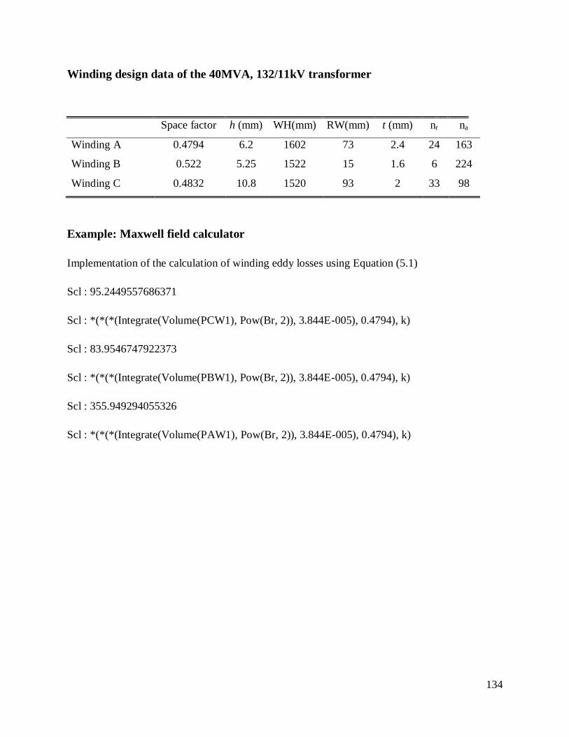
134
Winding design data of the 40MVA, 132/11kV transformer
Space factor h (mm) WH(mm) RW(mm) t (mm) nr na
Winding A 0.4794 6.2 1602 73 2.4 24 163
Winding B 0.522 5.25 1522 15 1.6 6 224
Winding C 0.4832 10.8 1520 93 2 33 98
Example: Maxwell field calculator
Implementation of the calculation of winding eddy losses using Equation (5.1)
Scl : 95.2449557686371
Scl : *(*(*(Integrate(Volume(PCW1), Pow(Br, 2)), 3.844E-005), 0.4794), k)
Scl : 83.9546747922373
Scl : *(*(*(Integrate(Volume(PBW1), Pow(Br, 2)), 3.844E-005), 0.4794), k)
Scl : 355.949294055326
Scl : *(*(*(Integrate(Volume(PAW1), Pow(Br, 2)), 3.844E-005), 0.4794), k)

135
Appendix D
Load loss test reports
Transformer 1 of Table 6.1
Courtesy of Powertech Transformers

136
Transformer 9 of Table 6.1
Courtesy of Powertech Transformers