The Competitiveness of Nations: Economic Growth in the ECE Region

By Jan Fagerberg, Mark Knell and Martin Srholec, Globalization Program, Centre for

Technology, Innovation and Culture, University of Oslo

Address for correspondence: jan.fagerberg@tik.uio.no

January 30, 2004

Abstract Why do some countries grow much faster, and have much better trade performance, than

other countries? What are the crucial factors behind such differences, and what can

governments do in order to improve the relative position of their economies? This paper

outlines a synthetic framework, based on Schumpeterian logic, for analysing such questions.

Four different aspects of competitiveness are identified; technology, costs, capacity and

demand. The framework is applied to a sample of 49 countries between 1993 and 2001.

Paper prepared for presentation at the UNECE Spring Seminar, Competitiveness and Economic Growth in the ECE Region, Geneva, February 23, 2004

1

1. Introduction

Why do some countries grow so much faster, and have much better trade performance, than

other countries? What are the crucial factors behind such differences? Which policies can

governments pursue to improve the relative performance of their economies (and welfare of

its citizens)? These are the kind of questions that motivate a concern for the competitiveness

of countries. Although the concept as such has been strongly criticized by some theoreticians

(see, e.g., Krugman 1994), the importance of the underlying challenges makes it unlikely that

this issue will lose the attention of policy makers soon.

We begin the paper with a few reflections on the concept of competitiveness and its use. First,

the concept it is applied on several levels. What has been the prime focus of the debate, and

what we will focus on here, is when applied to a country. Second, it is a relative term. What

is of interest is not absolute performance, however that may be defined, but how well a

country does relative to others. Some dislike this comparative perspective. But, after all, this

is a perspective that we find in nearly all aspects of social life, work, sports, business etc.,

among individuals as well as collectives. So why not at the level of countries? We see no

compelling reason not to use the concept at that level. Third, when applied to a country, it has

a double meaning, it relates both to the economic well-being of its citizens, normally

measured through GDP per capita, and the trade performance of the country.1 The underlying

assumption, then, is that these things are intimately related. This is perhaps not so

controversial in itself, but the precise nature of this relationship may of course be (see

Fagerberg 1996 for an extended discussion). In the next section we outline an analytical

1 There are many definitions around, most of which reflect this “double meaning” in one way or another. A typical example is the following: Competitiveness is “the degree to which, under open

2

framework, based on Schumpeterian logic, which among other things explains why, in

analyses of competitiveness, it is indeed natural to focus on both GDP and trade performance

and their mutual relationship.

Arguably, the discussion of the competitiveness issue has been much obscured by a common

tendency among many economists to focus on extremely simplified representations of reality

that abstracts from the very facts that make competitiveness an important issue for policy

makers and other stakeholders in a country. A well-known example of this is the idea of

“perfect competition”, which among other things presupposes that all agents have access to

the same body of knowledge, produce goods of identical quality and sell these in price-

clearing markets, so that the only thing left to care about is to get the price right. For a long

time this led applied economists and analysts to focus on price as the only aspect of

competitiveness. Joseph Schumpeter long ago described the short-comings of such

simplifications. The true nature of capitalist competition, he argued, is not price competition,

as envisaged in traditional text- books, but technological competition:

“But in capitalist reality as distinguished from its textbook picture, it is not that kind of

competition that counts but the competition from the new commodity, the new

technology, the new source of supply, the new type of organization (…) - competition

which commands a decisive cost or quality advantage and which strikes not at the

margins of the profits and the outputs of the existing firms but at their foundations and

their very lives. ” (Schumpeter 1943, p. 84)

market conditions, a country can produce goods and services that meet the test of foreign competition while simultaneously maintaining and expanding domestic real income” (OECD 1992, p. 237).

3

In this paper we depart from the “perfect competition” approach and the idea of technology as

a public good. Rather, following Dosi (1988) and others, we assume that technology is

cumulative and context dependent in ways that prevent the economic benefits of innovation to

spread more or less automatically. This more realistic approach to the role of technology in

economic change does not prevent diffusion from being a powerful factor behind growth and

competitiveness in so-called latecomer countries (see Fagerberg and Godinho 2004). On the

contrary we side with the economic historian Gerschenkron (1962) in his suggestion that the

technological gap between a frontier and a latecomer country represents “a great promise” for

the latter, since it provides the latecomer with the opportunity of imitating more advanced

technology in use elsewhere. However, just as he and others have done (see Abramovitz

1986, 1994), we stress the stringent requirements for getting the most out of such

opportunities. In fact, this holds not only for latecomer countries, but also for countries closer

to or on the frontier, since similar considerations apply for the successful commercialisation

all new technologies, independent of where it was first developed. We use the term “capacity

competitiveness” for this aspect of the competitiveness of a country, which we suggest to

consider in addition to the two other aspects – technology and price competitiveness –

mentioned above. Finally, following one of the suggestions in the literature on

competitiveness (see the next section), we also take into account the ability of a country to

exploit the changing composition of demand, by offering attractive products that are in high

demand at home and abroad. We label this (fourth) aspect “demand competitiveness”.

The main objective of this paper is to analyse the competitive performance of the countries in

the ECE region between 1993 and 2001 with respect to the four dimensions of

competitiveness outlined above. First, however, we outline a synthetic framework, based on

4

Schumpeterian logic, which explains how these different aspects feed into the overall

competitiveness of a country.

2. A synthetic framework

We start by developing a very simple growth model based on Schumpeterian logic, which we

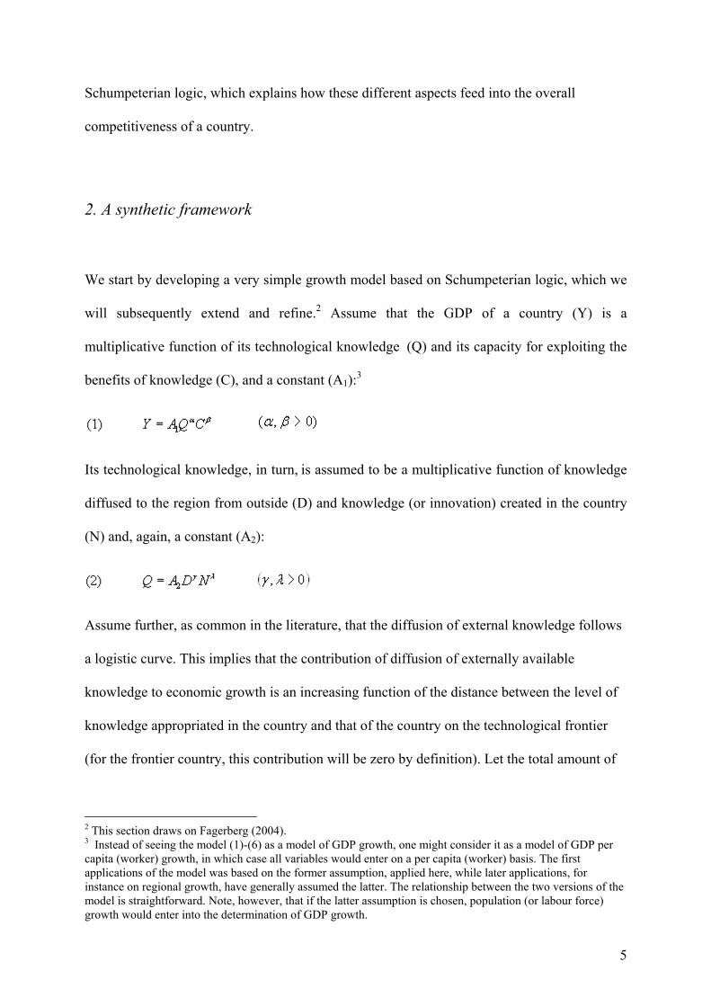
will subsequently extend and refine.2 Assume that the GDP of a country (Y) is a

multiplicative function of its technological knowledge (Q) and its capacity for exploiting the

benefits of knowledge (C), and a constant (A1):3

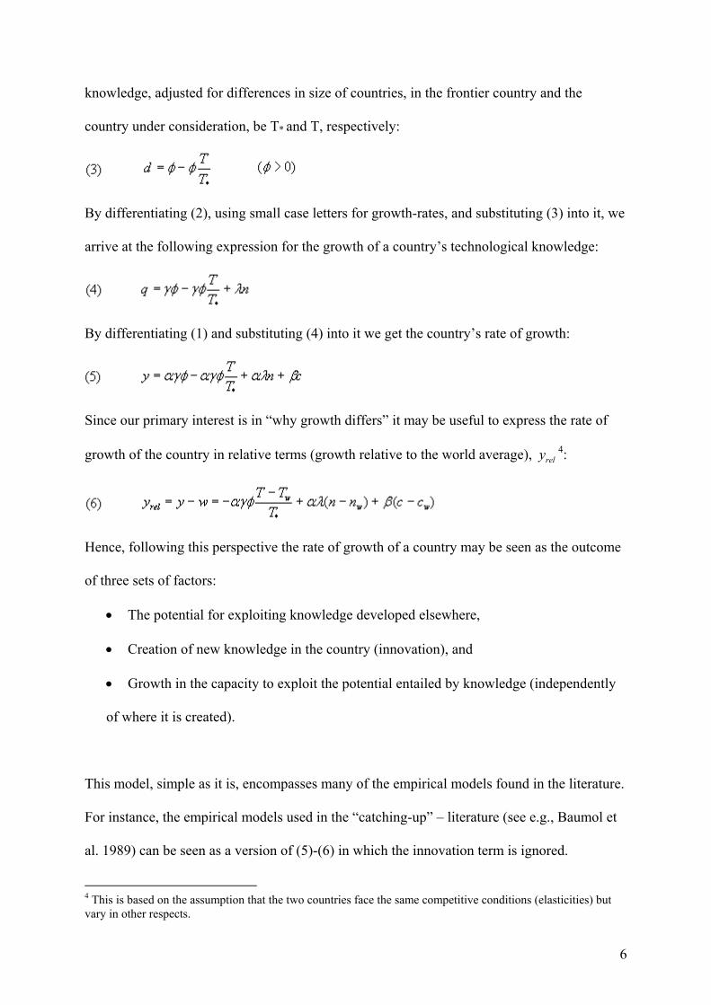
Its technological knowledge, in turn, is assumed to be a multiplicative function of knowledge

diffused to the region from outside (D) and knowledge (or innovation) created in the country

(N) and, again, a constant (A2):

Assume further, as common in the literature, that the diffusion of external knowledge follows

a logistic curve. This implies that the contribution of diffusion of externally available

knowledge to economic growth is an increasing function of the distance between the level of

knowledge appropriated in the country and that of the country on the technological frontier

(for the frontier country, this contribution will be zero by definition). Let the total amount of

2 This section draws on Fagerberg (2004). 3 Instead of seeing the model (1)-(6) as a model of GDP growth, one might consider it as a model of GDP per capita (worker) growth, in which case all variables would enter on a per capita (worker) basis. The first applications of the model was based on the former assumption, applied here, while later applications, for instance on regional growth, have generally assumed the latter. The relationship between the two versions of the model is straightforward. Note, however, that if the latter assumption is chosen, population (or labour force) growth would enter into the determination of GDP growth.

5

knowledge, adjusted for differences in size of countries, in the frontier country and the

country under consideration, be T* and T, respectively:

By differentiating (2), using small case letters for growth-rates, and substituting (3) into it, we

arrive at the following expression for the growth of a country’s technological knowledge:

By differentiating (1) and substituting (4) into it we get the country’s rate of growth:

Since our primary interest is in “why growth differs” it may be useful to express the rate of

growth of the country in relative terms (growth relative to the world average), rely 4:

Hence, following this perspective the rate of growth of a country may be seen as the outcome

of three sets of factors:

• The potential for exploiting knowledge developed elsewhere,

• Creation of new knowledge in the country (innovation), and

• Growth in the capacity to exploit the potential entailed by knowledge (independently

of where it is created).

This model, simple as it is, encompasses many of the empirical models found in the literature.

For instance, the empirical models used in the “catching-up” – literature (see e.g., Baumol et

al. 1989) can be seen as a version of (5)-(6) in which the innovation term is ignored.

4 This is based on the assumption that the two countries face the same competitive conditions (elasticities) but vary in other respects.

6

Fagerberg (1987, 1988a) applied this model to a sample of developed and medium-income

countries. It was shown that countries that caught up very fast, also had very rapid growth of

innovative activity. The analysis presented in Fagerberg (1988a) suggested that superior

growth in innovative activity was the prime factor behind the huge difference in performance

between Asian and Latin-American NIC-countries in the 1970s and early 1980s. Fagerberg

and Verspagen (2002) likewise found that the continuing rapid growth of the Asian NICs

relative to other country groupings in the decade that followed was primarily caused by the

rapid increases in its innovative performance. Estimations of the model for different time

periods (Fagerberg 1987, Fagerberg and Verspagen 2002) have shown that while imitation

has become more demanding over time (and hence more costly to undertake), innovation has

become a more powerful factor in explaining observed differences in growth performance.

The model opens up for international technology flows but abstracts from flows of goods and

services. We will now introduce the latter. For simplicity we do this in a two-country

framework, in which the other country is labelled “world”. Define the share of a country’s

exports (X) in world demand (W) as WXSx /= , and similarly the share of imports (M) in its

own GDP (Y) as . For the sake of exposition we assume that the market shares of

a country are unaffected by the growth of the market, but we will relax this assumption later.

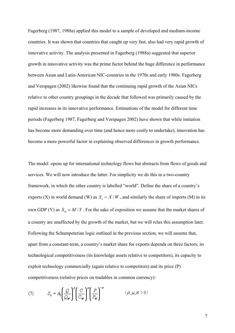
Following the Schumpeterian logic outlined in the previous section, we will assume that,

apart from a constant-term, a country’s market share for exports depends on three factors; its

technological competitiveness (its knowledge assets relative to competitors), its capacity to

exploit technology commercially (again relative to competitors) and its price (P)

competitiveness (relative prices on tradables in common currency):

YMSm /=

7

Since, by definition, imports in this model are the “world”’s exports, we may model the

import share in the same way, using bars to distinguish the coefficients of the two equations:

By differentiating (7) and substituting (4) into it, and similarly for (8), we arrive at the

dynamic expressions for the growth in market shares:

We see that the growth of the market share of a country depends on four factors:

• The potential for exploiting knowledge developed elsewhere, which depends on the

country’s level of technological development relative to the world average.

• Creation of new knowledge (technology) in the country (innovation) relative to that of

competitors.

• Growth in the capacity exploit knowledge, independently of where it is created,

relative to that of competitors.

• Change in relative prices in common currency .

Following Thirlwall (1979) and Fagerberg (1988b) we now introduce the requirement that

trade in goods and services has to balance (if not in the short, so in the long run). Countries

may, however, have foreign debts (or assets). As is easily verified, we may multiply the left or

right hand side of (11) with a scalar without any consequence for the subsequent deductions.

Hence an alternative way to formulate this restriction might be that the deficit (surplus) used

to service foreign debt (derived from assets abroad) should be a constant fraction of exports

(or imports).

8

By differentiating (11), substituting and into it and rearranging we arrive at the

dynamic form of the restriction:

XS MS

This assumption has been extensively tested on data for developed economies and found to

hold well (Fagerberg 1988b, Meliciani 2001).

By substituting (9)-(10) into (12) and rearranging we get the reduced form of the model:

By comparing this with the similar reduced form of the growth model (6) we see that, apart

from the last term on the right hand side, the model has the same structure. The only

difference is that the coefficients of the basic growth equation now are shown to be sums of

coefficients for the similar variables in the market-share equations (for the domestic and

world market). Hence, the sensitivity of the markets (or “selection environments”) for new

technologies clearly matters for growth. The final term is the familiar Marshall-Lerner

condition which states the sum of the price-elasticities for exports and imports (when

measured in absolute value) has to be higher than one if deteriorating price-competitiveness is

going to harm the external balance (and – in this case – the rate of growth of GDP).

We have modelled the market share equations on the assumption that, when not only price,

but also technology and capacity have been taken into account as competitive factors, demand

may be assumed to have a unitary elasticity. This means, for instance, abstracting from other

factors, that if export demand grows by a certain percentage, exports will do the same, so that

the market share remains unaffected. However, there are reasons to believe that this

9

assumption, although appealing in its simplicity, does not necessarily hold in reality. For

instance, it has been argued that if a country has a pattern of specialization geared towards

industries that are in high (low) demand internationally its exports may grow faster (slower)

than world demand, quite independently of what happens to other factors (Thirlwall 1979,

Kaldor 1981). This way of reasoning, distinctly Keynesian in flavour, place more emphasis on

the growth world demand, and on the “income elasticities of demand” for a country’s exports

and imports, in determining a country’s growth performance.5 The higher the income

elasticity of exports relative to that of imports, it is argued, the higher the rate of growth will

be, and vice versa. Arguably, this might be expected to be of greatest relevance for small

countries, since these are likely to be more specialised in their economic (and trade) structure

than large ones. To take this possibility into account we, following Fagerberg (1988b),

introduce demand in the market shares equations:

By differentiating and substituting we arrive at the following expression for the reduced form:

(13')

The first thing to note is that the higher the demand elasticity for imports, the lower the effect

on growth of all other factors. The second is, as before, that while the first three terms on the

right hand side resemble the basic growth model (6), the two last terms in (13') resemble the

5 The income elasticity of exports is the growth in exports resulting from a 1% increase in world demand, holding relative prices constant (and ignoring cyclical factors). Similarly for imports.

10

model suggested by Thirlwall (1979). Hence, both the basic model (6) and Thirlwall’s model

can be seen as special cases of a more general, open-economy model.6

3. The competitiveness of the countries of the ECE region 1993 – 2001:

the “stylized facts”

The open-economy model, outlined above, has been applied to empirical data for developed

economies by Fagerberg (1988b). Based on data for fifteen OECD countries from the early

1960s to the early 1980s, the empirical results generally confirmed the importance of growth

in technological and productive capacity for competitiveness. The impact of price or cost

factors was found to be relatively marginal, consistent with the earlier findings by Kaldor (the

so-called Kaldor paradox, see Kaldor 1978). 7 Recently, Meliciani (2001) has applied the

model to a longer time series, including a more recent time period, with broadly similar

results.8 In this paper we move significantly beyond these previous empirical applications of

this perspective. First we consider a much broader sample, 49 countries, characterized by very

different development levels and trends, for a more recent (though shorter) time span (1993-

2001). The sample consists of all ECE countries for which data were available, supplemented

by some Asian and Latin American countries. The non-member countries were included

partly for a comparative purpose, but also because some these countries during the last few

6 If the demand elasticities are the same in both markets and the Marshall-Learner conditions is exactly satisfied (or relative prices do not change), the two last terms vanish, and we are back in a model that for all practical purposes is identical to (6). If, on the other hand, the country’s technological level is exactly average and both relative technology and relative capacity keep constant, the three first terms vanish, and only Thirlwall’s model remains. 7 Kaldor (1978) showed for a number of countries that over the long term market shares for exports and relative unit costs or prices tend to move together, i.e., that growing market shares and increasing relative costs or prices tend to go hand in hand. This was, of course, the opposite of what you would expect from the simplistic though at the time widely diffused approach focusing exclusively on the (assumedly negative) impact of increasing relative costs or prices on market shares, hence the term “paradox”. Fagerberg (1996) has shown that this finding also applies to a more recent time period.

11

decades have become very important players in the global economy. Second, and of even

greater importance, we develop much more sophisticated indicators of the various aspects that

together determine the overall competitiveness of a country. This is particularly the case for

“technology competitiveness” and “capacity competitiveness”, both of which are

multidimensional in character and consequently hard to measure. But we also develop a new

indicator of “demand competitiveness” that in a better way captures the underlying ideas

behind the inclusion of this particular dimension.

Figure 1 presents some basic data on development levels and trends for the countries included

into our investigation. While the vertical axis measures average productivity or income over

the period (GDP per capita in PPPs in 1997), the horizontal axis reports annual average

growth over the period (1993-2001). By combining these two aspects, level and trend, four

different quadrants emerge. First, to the upper left we have countries with a high level GDP

per capita but relatively slow growth, e.g., countries that “lose momentum”. The USA, Japan

and Switzerland are the prime examples. In contrast, in the upper left quadrant, we have

countries that continue to grow fast despite a high level of GDP per capita (“moving ahead”).

The most spectacular example is Ireland, other countries included in this more dynamic

category are Finland, Singapore and Taiwan. However, most developed countries, including

all the remaining EU members, cluster on the borderline between “losing momentum” and

“moving ahead”, indicating a growth performance close to the average of the sample.

8 She also added a “specialization” variable, reflecting the extent to which countries were specialized in technologically progressive sectors, to the market share equations, for which she found empirical support.

12

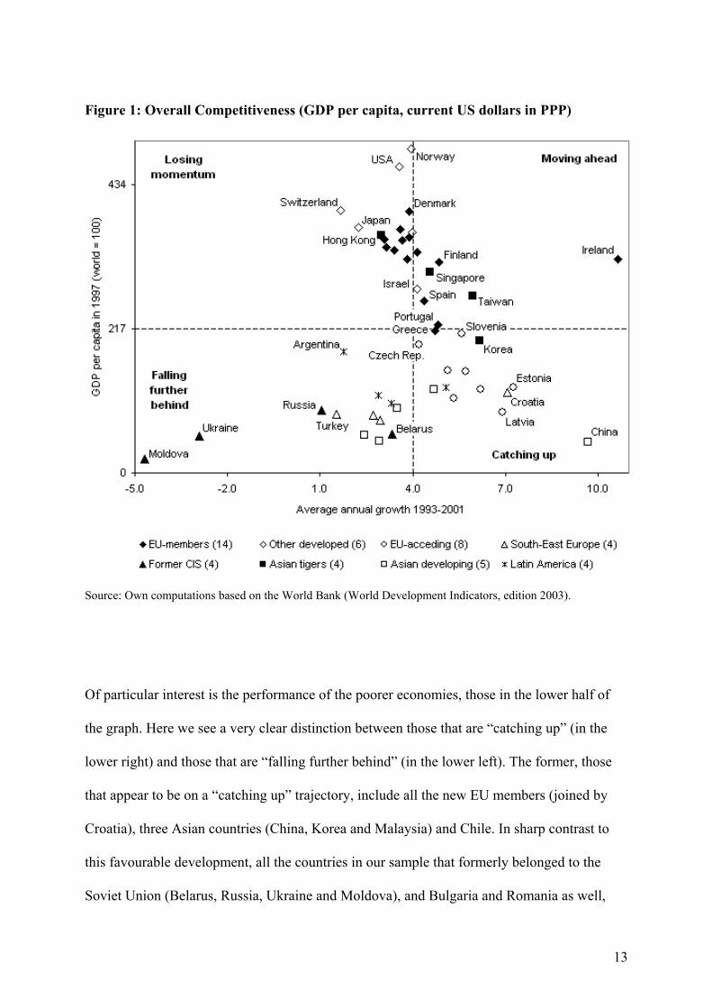
Figure 1: Overall Competitiveness (GDP per capita, current US dollars in PPP)

Source: Own computations based on the World Bank (World Development Indicators, edition 2003).

Of particular interest is the performance of the poorer economies, those in the lower half of

the graph. Here we see a very clear distinction between those that are “catching up” (in the

lower right) and those that are “falling further behind” (in the lower left). The former, those

that appear to be on a “catching up” trajectory, include all the new EU members (joined by

Croatia), three Asian countries (China, Korea and Malaysia) and Chile. In sharp contrast to

this favourable development, all the countries in our sample that formerly belonged to the

Soviet Union (Belarus, Russia, Ukraine and Moldova), and Bulgaria and Romania as well,

13

continue to fall further behind. This unfavourable performance is shared with, among others,

some of the Asian and Latin-American countries included in our sample.

Clearly there is a lot of diversity in how countries perform. Although in each and every case

there will be specific factors at work these will not be in focus here. Rather what we will

attempt, in a better way than in previous analyses, to single out some general factors that may

be of interest when discussing the wide differences across countries in economic

performance. These are, as noted,

- technology competitiveness,

- capacity competitiveness,

- cost competitiveness, and

- demand competitiveness.

Of these the two former are clearly multi-dimensional and therefore more difficult to handle.

Our approach here will be to identify the most important dimensions, find reliable indicators,

express these in a comparable format and weigh them together, giving each dimension an

equal weight in the calculation of the composite indicator.9 A complete list with definitions

and sources for the indicators used is given in appendix. In some cases, missing data had to be

estimated. Whenever possible, indicators are defined as activities measured in quantity or

constant prices, deflated by population. To further increase comparability we normalize the

indicators as follows:

9 Admittedly, there is an element of arbitrariness involved here. It would of course have been preferable to have prior knowledge about the “true weights” to use. Having no such information, we chose to give each variable an equal weight. Alternatively, one might have weighted variables based on the degree of correlation, based on the assumption that correlated variables express aspects of the same underlying phenomenon, in contrast to uncorrelated ones that are assumed to refer to different phenomena (as done in so-called “factor analysis”, for instance). Correlation and causation are not the same, however. For instance, in our case ICT-use and corruption are highly correlated, without any obvious causal relationship. In contrast, our two measures of technology diffusion, investments and fees/payments for use of proprietary technology, are almost uncorrelated. See European Commission (2002) and Freudenberg (2003) for an extended discussion.

14

deviationdardsvaluemeanvalueactual

tan−

In the calculations the mean and standard deviation were fixed to that of the median year

(1997). This means that changes over time in the volume of the activities measured by the

individual indicators are allowed to spill over to the composite indicator (along with the

changes caused by shifts in the position of countries on each individual indicator). For

instance, in the early 1990s ICT diffusion was still at a relatively low level. Today ICT

technologies are very widely used and are, arguably, of much higher importance to

competitiveness than it was a decade ago. The way we calculate the capacity indicator is

consistent with this.

Technology competitiveness

Technology (or technological) competitiveness refers to the ability to compete successfully in

markets for new goods and services. Hence, this type of competitiveness is closely related to

the innovativeness of a country. There is, however, no available data source which measures

innovativeness directly. Instead what we have are different data sources reflecting different

aspects of the phenomenon. R&D expenditures, for instance, measure some (but not all) of

the resources that go into developing new goods and services. Patent statistics, on the other

hand, measure the output of (patentable) inventions. This is a very reliable indicator, but the

propensity to patent varies considerably across industries, and many innovations are not

patentable. So a lot of innovation would get unaccounted for by using this indicator only.

Taking into account both indicators clearly gives a more balanced picture. To further increase

the reliability of the composite indicator we also include a measure of the quality of the

15

science base on which innovation activities depend as reflected in articles published in

scientific and technical journals.

Figure 2: Overall and Technology Competitiveness (average levels 1993-2001)

Source: Own computations based on the World Bank (WDI, edition 2003), OECD (MSTI and Patent data), UNESCO and RICYT.

16

Figure 3: Technology Competitiveness

Source: Own computations based on the World Bank (WDI, edition 2003), OECD (MSTI and Patent data), UNESCO and RICYT.

Figure 2 plots technology competitiveness on the horizontal axis against overall

competitiveness, as reflected in GDP per capita, on the vertical axis. As is evident from the

regression-line there is a very close correlation between overall and technological

competitiveness. The main deviants are some former centrally planned economies (headed by

Moldova) and developing countries in Asia, all of which with GDP per capita levels much

17

below what should be expected from their levels of technology competitiveness. But there are

also some small advanced countries for which GDP per capita tend to lag behind

technological competitiveness (Sweden and Israel in particular). On the other side of the

spectrum, Norway and Hong Kong are examples of countries that have managed to arrive at

relatively high levels of productivity and income without a similarly high technology

competitiveness.

In figure 3 the level and trend in technology competitiveness is plotted against each other.

When compared with the case of overall competitiveness in Figure1, the indicator for

technological competitiveness displays a much stronger tendency towards divergence.

Countries either move ahead of the others or fall further behind, with only a few staying in the

middle. Among the countries that move ahead technologically, Taiwan, Finland, Sweden and

Israel are most prominent. Those falling further behind include the former centrally planned

economies (with Slovenia as the only exception) and the developing countries in Asia and

Latin-America.

Capacity Competitiveness

The distinction between technology competitiveness and capacity competitiveness is crucial.

For instance, Sony did not develop the transistor, but showed a superior capacity to US firms

when it came to exploiting this new technology in a way that sustained competitiveness. In

fact, many of the inroads of Japanese producers on Western markets during most of the post-

war period were of this kind. Although the distinction may be clear enough in theory, in

practice it may not be all that simple, since resources that are devoted to developing new

goods and services may also be beneficial for the ability to exploit such innovations

18

economically (Cohen and Levinthal 1990) and vice versa. Nevertheless, we will focus on four

dimensions of capacity competitiveness, as distinct from technology competitiveness. These

four dimensions are human capital, ICT infrastructure, diffusion and social and institutional

aspects. The importance of a well developed human capital base for exploiting technological

opportunities goes without saying; here we focus on secondary and tertiary education (as

reflected in enrolment rates) in particular. Similarly, a well developed ICT infrastructure is

generally acknowledged as a must, we measure this with the help of data on the spread of

computers and telecommunication technologies across the population. However, the

importance of diffusion – or the ability to quickly put new technologies into use - extends

beyond that of ICT. We take this into account in two ways, as embodied in investments and

disembodied through payments of royalty or license fees. Finally, we acknowledge that there

may be a number of social and institutional factors of importance for the capacity to exploit

technological opportunity. Although such factors often defy measurement, at least on a broad

cross-country/cross-temporal basis, there exist survey-data on the incidence of corruption

across countries, which is relevant to consider.

19

Figure 4: Overall and Capacity Competitiveness (average levels 1993-2001)

Source: Own computations based on the World Bank (WDI, edition 2003), UNESCO, USAID (Global Education Database), ITU (World Telecommunication Indicators) and Transparency International (Corruption Perception Index).

Figure 4 plots our estimate of capacity competitiveness (horizontal axis) against overall

competitiveness as reflected in GDP per capita (vertical axis). As with technology

competitiveness there is a very clear, positive relationship between capacity competitiveness

and GDP per capita. The fit is even better than in the previous case, 86 per cent of the

differences in GDP per capita across countries can be explained by differences in the capacity

20

to exploit technological opportunity (against 70 per cent for technology competitiveness).

Consistent with this close fit there are few obvious deviants, with the possible exception of

Ireland, which reports a much higher capacity for exploiting technology than indicated by its

GDP per capita. Figure 5, which plots the level and trend of capacity competitiveness against

each other, confirms the peculiar Irish pattern, with a very high and growing level of capacity

for exploiting new technology. Hence, Ireland appears to an example of a country that has,

with considerable success, focused mainly at developing capacity competitiveness at the

possible expense of technological competitiveness. This contrasts with position of a number

of other economies, such as Switzerland, Israel and Japan, which - although technologically

advanced - appear to have less well developed capabilities for exploiting these advantages

commercially (Figure 6).

21

Figure 5: Capacity Competitiveness

Source: Own computations based on the World Bank (WDI, edition 2003), UNESCO, USAID (Global Education Database), ITU (World Telecommunication Indicators) and Transparency International (Corruption Perception Index).

22

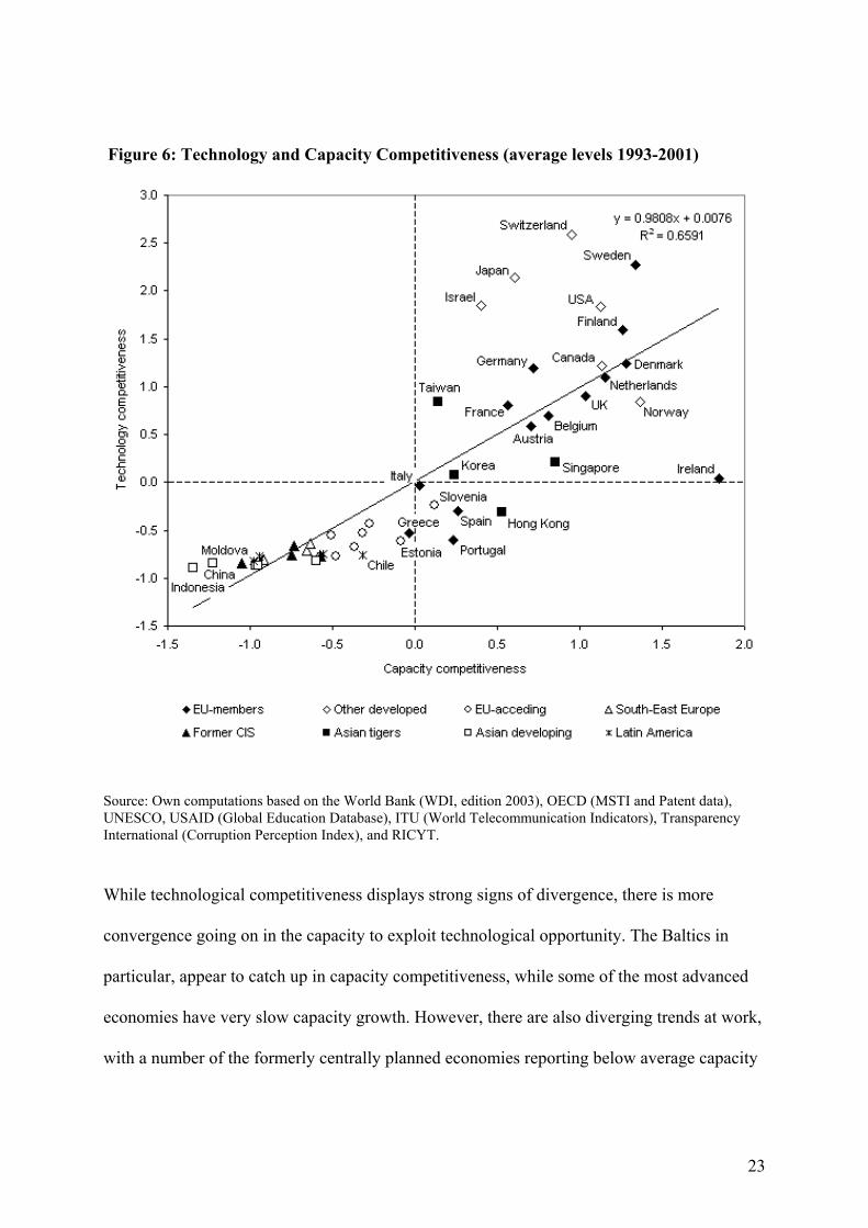
Figure 6: Technology and Capacity Competitiveness (average levels 1993-2001)

Source: Own computations based on the World Bank (WDI, edition 2003), OECD (MSTI and Patent data), UNESCO, USAID (Global Education Database), ITU (World Telecommunication Indicators), Transparency International (Corruption Perception Index), and RICYT.

While technological competitiveness displays strong signs of divergence, there is more

convergence going on in the capacity to exploit technological opportunity. The Baltics in

particular, appear to catch up in capacity competitiveness, while some of the most advanced

economies have very slow capacity growth. However, there are also diverging trends at work,

with a number of the formerly centrally planned economies reporting below average capacity

23

growth, and the same holds for most of the developing Asian and Latin American countries

included in our sample.

Price competitiveness

In one sense price- or cost competitiveness should be the easiest dimension to identify. In

fact, for a long time economists focused only on price or cost competitiveness, and a well

defined indicator – unit labour costs in manufacturing in a common currency – was readily

available. We, however, found that indicator to be one of the most problematic in terms of

data coverage. The estimates of price or cost competitiveness (unit wage costs in

manufacturing) presented here are based on several sources and considerable judgement had

to be made in order to improve the coverage (see the appendix for further details). Among

other things indirect wage costs (benefits etc.) could not be taken into account due to lacking

data for many countries. Hence the estimates presented should be interpreted with

considerable care

Figure 7 plots price competitiveness, measured as unit wage costs in manufacturing

(horizontal axis) against overall competitiveness, measured through GDP per capita (vertical

axis). As is evident from the figure there generally is a positive relationship as should be

expected; more advanced (richer) economies, using highly qualified labour, generally pay

higher wages per unit produced than do less developed, poorer countries. There is, however,

considerable variation around the regression line. For instance, some developed economies,

such as Ireland, Switzerland, USA and Norway, consistently have higher productivity levels

24

than indicated by their price or cost competitiveness, while for some formerly centrally

planned economies the situation is the other way around.10

Figure 7: Overall and Price Competitiveness (average levels 1993-2001)

Source: Own computations based on the World Bank (WDI), OECD (STAN Database), ILO (LABORSTA Database), Eurostat (AMECO) and WIIW (WIIW Industrial Database Eastern Europe).

10 This may reflect differences in exchange-rates. While GDP per capita is measured in PPPs, wages are measured in current exhange-rates, which in several countries have been regulated to encourage exports and attract inflows of foreign capital.

25

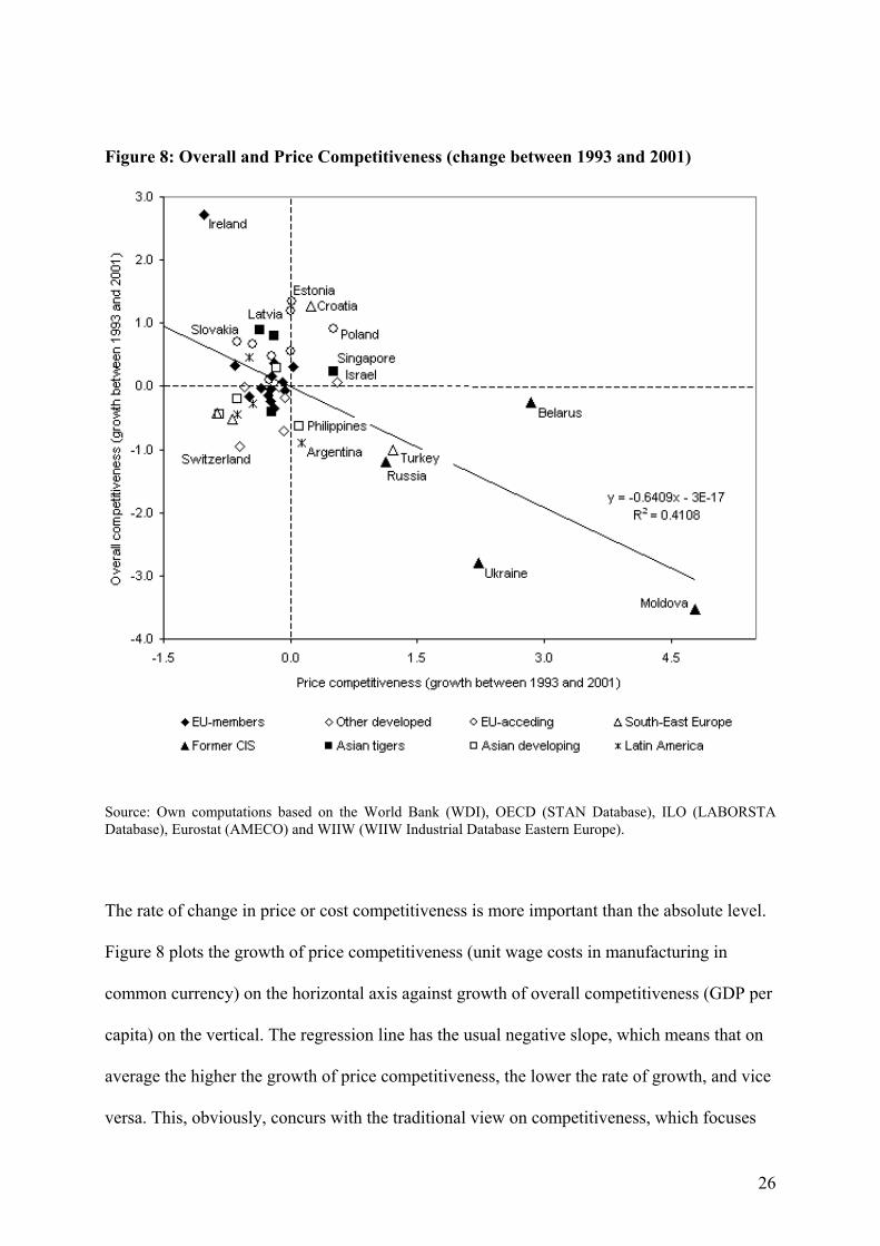
Figure 8: Overall and Price Competitiveness (change between 1993 and 2001)

Source: Own computations based on the World Bank (WDI), OECD (STAN Database), ILO (LABORSTA Database), Eurostat (AMECO) and WIIW (WIIW Industrial Database Eastern Europe).

The rate of change in price or cost competitiveness is more important than the absolute level.

Figure 8 plots the growth of price competitiveness (unit wage costs in manufacturing in

common currency) on the horizontal axis against growth of overall competitiveness (GDP per

capita) on the vertical. The regression line has the usual negative slope, which means that on

average the higher the growth of price competitiveness, the lower the rate of growth, and vice

versa. This, obviously, concurs with the traditional view on competitiveness, which focuses

26

mainly on the damaging effects on the economy of excessive wage growth. Note, however,

that the estimated relationship depends to some extent on outliers (Moldova, Belarus, Ukraine

and Ireland). If these observations are excluded, the regression line becomes much flatter, and

the estimated coefficient no longer significant.

Demand competitiveness

The relationship between a country production (or trade) structure and the composition of

world demand may also be of importance for competitiveness. Better the match, the more

favourable the country’s economy should be supposed to develop, and vice versa. We capture

this aspect by weighting the growth of world demand (by commodity) by the commodity

composition of each country’s exports:

∑

=

n

1iiTijgw

where w is share of product group in country j, g is growth of the export market, i is product

group and T is market total.

Figure 9 plots the relationship between demand competitiveness, so defined (horizontal axis),

and growth of GDP per capita (vertical axis). It is evident from the regression included in the

figure that there is a positive albeit weak relationship between the two variables. Those that

appear to have gained most from the composition of demand were Ireland and some Asian

economies, while some former centrally planned economies, joined by Chile and Argentina,

were the least favourably affected

27

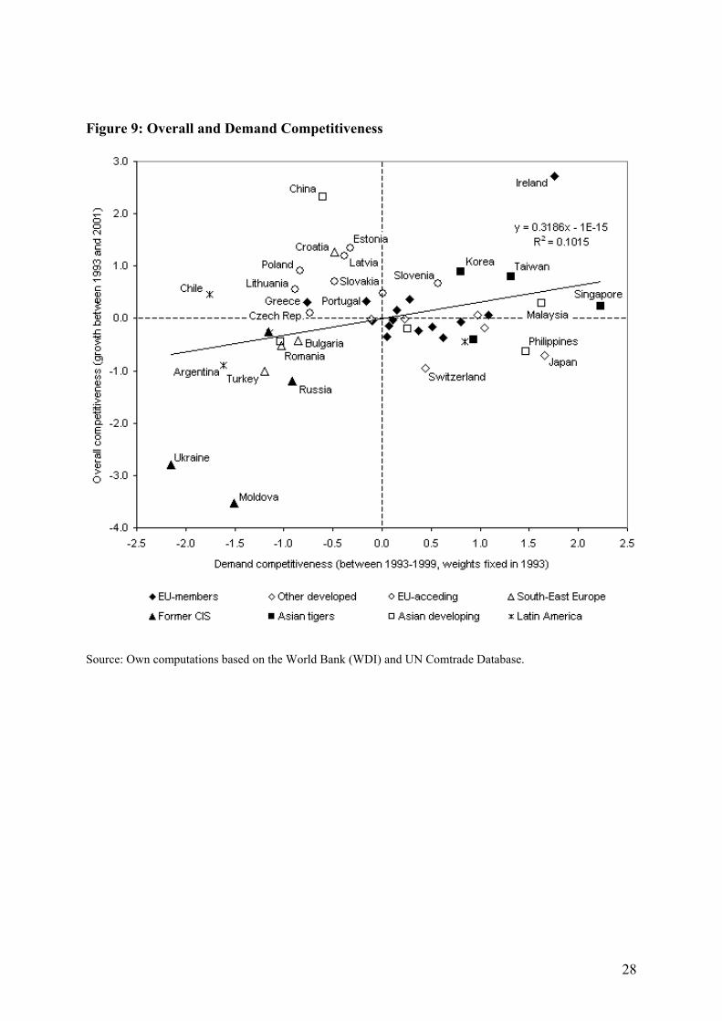
Figure 9: Overall and Demand Competitiveness

Source: Own computations based on the World Bank (WDI) and UN Comtrade Database.

28

3. The dynamics of the competitiveness of the countries of the ECE region

Having developed empirical indicators of the different aspects of competitiveness, we will

apply these indicators in an analysis of the differing performance of ECE countries. However,

the short time period for which (reliable) data are available (especially for many of the former

centrally planned economies) puts severe limits on the possibilities for econometric work.

We therefore refrained from estimating the entire model, and chose instead to concentrate on

its reduced form, as given by equation 13’, according to which the rate of economic growth of

a country should be a weighted sum of

- the potential for diffusion,

- growth in technological competitiveness,

- growth in capacity competitiveness,

- growth in cost competitiveness, and

- demand competitiveness, all relative to that of other countries.

The main purpose of the estimation, then, is to estimate these weights, which in turn will be

used to assess the impact of the different aspects of competitiveness on overall

competitiveness. To calculate the potential for diffusion we use, as in previous empirical

applications of this model, the difference between the level of GDP per capita in the country

and average GDP in our sample, deflated by the GDP per capita in the leader country. For the

other four variables we used the indicators developed in the previous section. However, the

normalization procedure used in creating the indicators of technology and capacity

competitiveness made it difficult to calculate growth rates. We therefore transformed the

29

normalized indicators to a series of positive numbers (by adding a sufficiently high positive

number11) before calculating the growth rates.

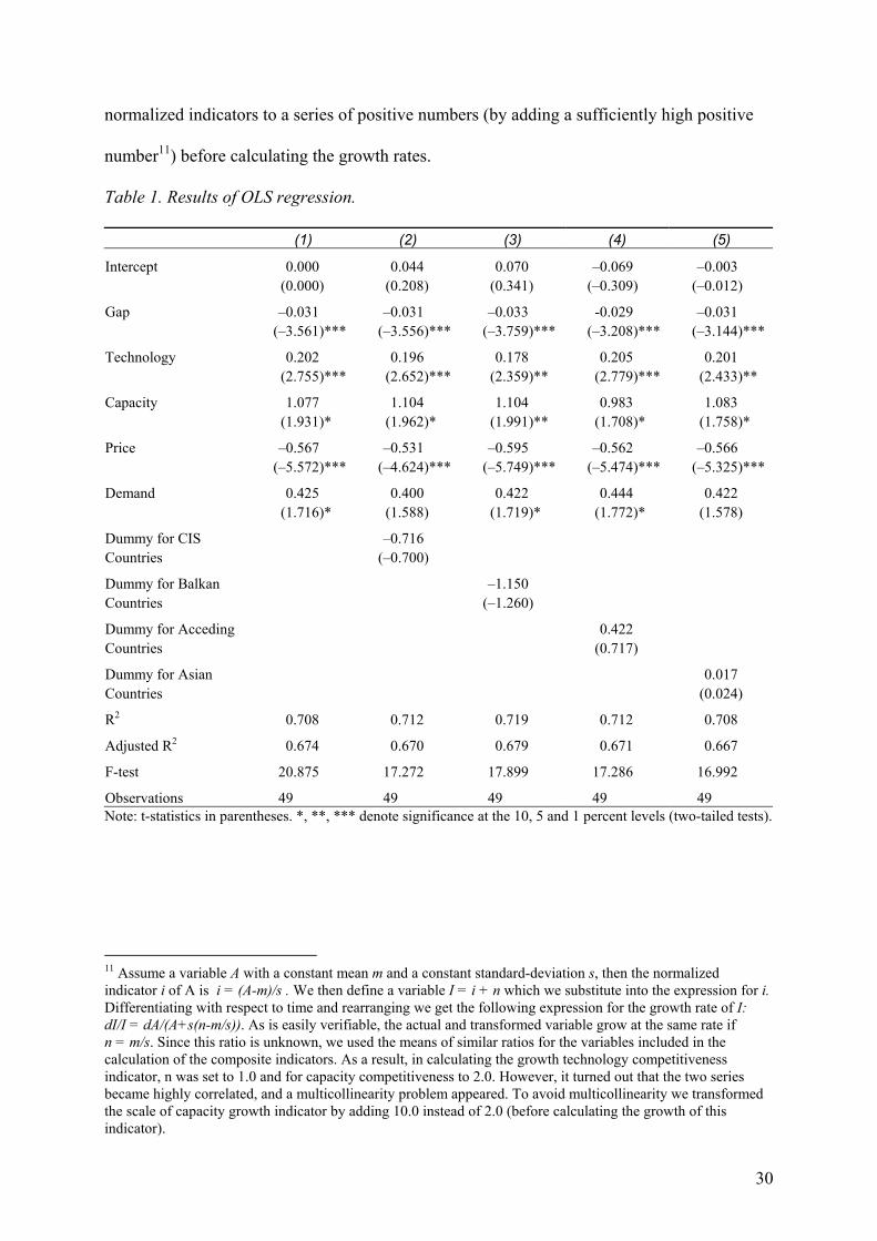
Table 1. Results of OLS regression.

(1) (2) (3) (4) (5)

Intercept 0.000 0.044 0.070 –0.069 –0.003 (0.000) (0.208) (0.341) (–0.309) (–0.012)

Gap –0.031 –0.031 –0.033 -0.029 –0.031 (–3.561)*** (–3.556)*** (–3.759)*** (–3.208)*** (–3.144)***

Technology 0.202 0.196 0.178 0.205 0.201 (2.755)*** (2.652)*** (2.359)** (2.779)*** (2.433)**

Capacity 1.077 1.104 1.104 0.983 1.083 (1.931)* (1.962)* (1.991)** (1.708)* (1.758)*

Price –0.567 –0.531 –0.595 –0.562 –0.566 (–5.572)*** (–4.624)*** (–5.749)*** (–5.474)*** (–5.325)***

Demand 0.425 0.400 0.422 0.444 0.422 (1.716)* (1.588) (1.719)* (1.772)* (1.578)

Dummy for CIS –0.716 Countries (–0.700)

Dummy for Balkan –1.150 Countries (–1.260)

Dummy for Acceding 0.422 Countries (0.717)

Dummy for Asian 0.017 Countries (0.024)

R2 0.708 0.712 0.719 0.712 0.708

Adjusted R2 0.674 0.670 0.679 0.671 0.667

F-test 20.875 17.272 17.899 17.286 16.992

Observations 49 49 49 49 49 Note: t-statistics in parentheses. *, **, *** denote significance at the 10, 5 and 1 percent levels (two-tailed tests).

11 Assume a variable A with a constant mean m and a constant standard-deviation s, then the normalized indicator i of A is i = (A-m)/s . We then define a variable I = i + n which we substitute into the expression for i. Differentiating with respect to time and rearranging we get the following expression for the growth rate of I: dI/I = dA/(A+s(n-m/s)). As is easily verifiable, the actual and transformed variable grow at the same rate if n = m/s. Since this ratio is unknown, we used the means of similar ratios for the variables included in the calculation of the composite indicators. As a result, in calculating the growth technology competitiveness indicator, n was set to 1.0 and for capacity competitiveness to 2.0. However, it turned out that the two series became highly correlated, and a multicollinearity problem appeared. To avoid multicollinearity we transformed the scale of capacity growth indicator by adding 10.0 instead of 2.0 (before calculating the growth of this indicator).

30

Table 1 presents the results of the regression analysis. The coefficients for the five variables

included in the model all have the expected signs, significantly different from zero at the 1 per

cent or 10 per cent level. The explanatory value is high, above 70 per cent. Since the period of

estimation was characterized by severe problems for some country groupings (the “Asian

crisis” for instance), we also test for the possible impact of this by including dummy variables

for relevant country groupings. As is evident from the table none of these dummies were

significant at conventional levels of significance, and the impact on the estimates for the other

variables was small, although the significance of the estimated coefficients declined in a few

cases (particularly for the demand variable).

To illustrate the implications of these estimates, we decomposed the estimated growth of GDP

(relative to the average of the sample) for eight different country groups into its constituent

parts (as explained by the estimated model and the relevant data). Table 2 ranks the eight

country groups after their initial GDP per capita, from highest to lowest. As is evident from

the table, the model captures most of the qualitative features, although the explanatory power

is not perfect, especially not for some of the richest countries in our sample (the so-called

“other developed” countries). The model predicts that these rich countries should be expected

to grow relatively slowly (as they on average do), mainly as a consequence of the lacking

diffusion potential and the failure to increase technology and capacity competitiveness

sufficiently to make up for this loss. However, the model fails to replicate “the new economy

boom” that some of these countries went through in the 1990s, and hence underestimates their

average growth during this period. The prediction is better for the EU countries, which also

benefit less than many others from the potential for diffusion. However, on average, for the

31

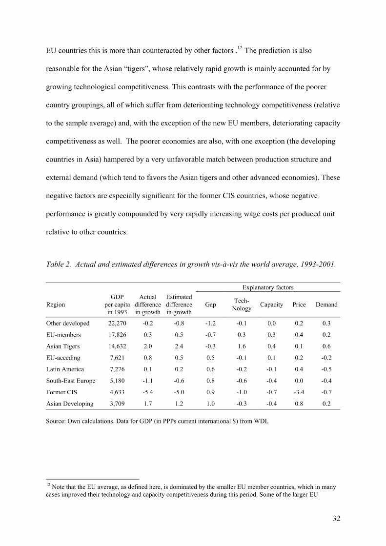
EU countries this is more than counteracted by other factors .12 The prediction is also

reasonable for the Asian “tigers”, whose relatively rapid growth is mainly accounted for by

growing technological competitiveness. This contrasts with the performance of the poorer

country groupings, all of which suffer from deteriorating technology competitiveness (relative

to the sample average) and, with the exception of the new EU members, deteriorating capacity

competitiveness as well. The poorer economies are also, with one exception (the developing

countries in Asia) hampered by a very unfavorable match between production structure and

external demand (which tend to favors the Asian tigers and other advanced economies). These

negative factors are especially significant for the former CIS countries, whose negative

performance is greatly compounded by very rapidly increasing wage costs per produced unit

relative to other countries.

Table 2. Actual and estimated differences in growth vis-à-vis the world average, 1993-2001.

Explanatory factors

Region GDP

per capita in 1993

Actual difference in growth

Estimated difference in growth

Gap Tech- Nology Capacity Price Demand

Other developed 22,270 -0.2 -0.8 -1.2 -0.1 0.0 0.2 0.3

EU-members 17,826 0.3 0.5 -0.7 0.3 0.3 0.4 0.2

Asian Tigers 14,632 2.0 2.4 -0.3 1.6 0.4 0.1 0.6

EU-acceding 7,621 0.8 0.5 0.5 -0.1 0.1 0.2 -0.2

Latin America 7,276 0.1 0.2 0.6 -0.2 -0.1 0.4 -0.5

South-East Europe 5,180 -1.1 -0.6 0.8 -0.6 -0.4 0.0 -0.4

Former CIS 4,633 -5.4 -5.0 0.9 -1.0 -0.7 -3.4 -0.7

Asian Developing 3,709 1.7 1.2 1.0 -0.3 -0.4 0.8 0.2 Source: Own calculations. Data for GDP (in PPPs current international $) from WDI.

12 Note that the EU average, as defined here, is dominated by the smaller EU member countries, which in many cases improved their technology and capacity competitiveness during this period. Some of the larger EU

32

4. Conclusions

The purpose of this paper has been to empirically scrutinize why some countries, with

particular emphasis on the ECE region, consistently outperform others. Our search was

guided by a theoretical perspective that places emphasis on the role played by four different

aspects of competitiveness; technology, capacity, costs and demand. The contribution of the

paper is particularly to highlight the two first aspects, which often tend to get lost because of

measurement problems.

Our empirical analysis, based on a sample of 49 countries between 1993 and 2001,

demonstrated the relevance of both technology and capacity competitiveness. The former is

the main explanation behind the continuing good growth performance of the “Asian tigers”

relative to other major country groups. Deteriorating capacity competitiveness, on the other

hand, is one of the main factors hampering low-income countries in Europe (the formerly

centrally planned economies in particular) and Asia in exploiting the potential for catch-up in

technology and income.

What are the crucial factors behind these developments, and what can governments do in

order to improve the relative position of their economies? To better deal with these questions

we illustrate in figure 10 the factors behind the observed changes over time in technology

and capacity competitiveness.

countries had a much bleaker performance, however, particularly France and Germany.

33

Figure 10: Contribution to Change of Technology and Capacity Competitiveness

Source: Own computations based on the World Bank (WDI, edition 2003), OECD (MSTI and Patent data), UNESCO, USAID (Global Education Database), ITU (World Telecommunication Indicators), Transparency International (Corruption Perception Index), and RICYT.

The differences across country groups are striking. As for technology competitiveness, there

is a clear divide between the advanced countries, with healthy and continuing increases, and

the rest of the world which, with a partial exception for the new EU members, are stagnant at

best. The “Asian tigers” stand out with the best performance. This difference (relative to other

developed countries) is not so much rooted in increases in R&D as in growing innovation

(measured by patents) and the development of the scientific infrastructure. A divide of a

different sort is clearly visible along the capacity dimension. In this case there actually is

some catch up along one dimension, human capital, particularly by the new EU members, and

the developing countries in Asia and Latin-America. This, however, is more than

counteracted by an increasing digital divide (ICT-infrastructure), caused by much higher

34

investments in ICT in the already developed economies and among the Asian Tigers than

elsewhere.

These trends points to the possibility of continuing divergence in the world economy, as

emphasized also by other recent studies (see, e.g., Fagerberg and Verspagen 2002). However,

at any time some countries manage to defy the trend, as the “Asian tigers” indeed have done

in latter half of the post second-world-war period (and Japan before them). In our sample it is

the group of former centrally planned economies countries that are about to join the European

Union that appear to have the best chance in that respect. These favourable prospects contrast

with those of a number of other former centrally planned economies, which appear to witness

deteriorating competitiveness along all our four dimensions. Clearly, if these countries are

ever going to catch up, they will have to find ways to break this vicious circle. Some of the

developing countries in Asia are growing fast but this growth has to large extent been based

on exploiting the diffusion potential through a low cost strategy. There is danger that some of

these countries may soon find themselves constrained by lagging technology and capacity

competitiveness.

References

Abramovitz, M. (1986), Catching Up, Forging Ahead, and Falling Behind, Journal of Economic

History 46: 386-406 Abramovitz, M. (1994), “The Origins of the Postwar Catch-Up and Convergence Boom”, in

Fagerberg, J.. B. Verspagen and N. von Tunzelmann (eds.) The Dynamics of Technology, Trade and Growth, Aldershot: Edward Elgar, pp. 21-52

Archibugi, D., Coco, A. (2003), A New Indicator of Technological Capabilities for Developed and Developing Countries (ArCo), Rio de Janeiro, The First International Globelics Conference.

Baumol, W.J., S. A. Batey Blackman and E. N. Wolff (1989), Productivity and American Leadership: The Long View, Cambridge, Mass., MIT Press

35

Cohen, W. and Levinthal, D. (1990) Absorptive Capacity: A New Perspective on Learning and Innovation, Administrative Science Quarterly, 35:123-13

Dosi, G. (1988) Sources, Procedures and Microeconomic Effects of Innovation, Journal of Economic Literature 26: 1120-71

European Commission (2002), State-of-the-art Report on Current Methodologies and Practices for Composite Indicator Development, Ispra, European Commission Joint Research Centre (JRC).

Fagerberg, J. (1987) A Technology Gap Approach to Why Growth Rates Differ, Research Policy 16: 87-99, reprinted as chapter 1 in Fagerberg, J. (2002) Technology, Growth and Competitiveness: Selected Essays, Cheltenham: Edward Elgar

Fagerberg, J. (1988a)”Why Growth Rates Differ,” in Dosi, Giovanni et al. (eds.), Technical Change and Economic Theory, London: Pinter, pp. 432-457

Fagerberg, J. (1988b) International Competitiveness, Economic Journal, 98: 355-374, reprinted as chapter 12 in Fagerberg, J. (2002) Technology, Growth and Competitiveness: Selected Essays, Cheltenham: Edward Elgar

Fagerberg, J. (1994) Technology and International Differences in Growth Rates, Journal of Economic Literature 32: 1147-75

Fagerberg, J. (1996) Technology and Competitiveness, Oxford Review of Economic Policy 12: 39-51, reprinted as chapter 16 in Fagerberg, J. (2002) Technology, Growth and Competitiveness: Selected Essays, Cheltenham: Edward Elgar

Fagerberg, J. (2004) The dynamics of technology, growth and trade: A Schumpeterian perspective, in Hanusch, H. and A. Pyka (eds.), Elgar Companion to Neo-Schumpeterian Economics, Edward Elgar, Cheltenham, 2004, forthcoming

Fagerberg, J., and B. Verspagen (2002), Technology-Gaps, Innovation-Diffusion and Transformation: An Evolutionary Interpretation, Research Policy, 31: 1291-1304

Fagerberg, J. and M. Godinho (2004), Innovation and catching-up, in Fagerberg, J, D. Mowery and R. Nelson, Oxford Handbook of Innovation, Oxford University Press, Oxford, forthcoming

Freudenberg, M. (2003), Composite Indicators of Country Performance: A Critical Assessment, Paris, OECD, STI Working Paper 2003/16.

Gerschenkron, A. (1962) Economic Backwardness in Historical Perspective, Cambridge, Mass: The Belknap Press

Kaldor, N. (1978) The effect of devaluations on trade in manufactures, in Further Essays on Applied Economics, London: Duckworth

Kaldor, N. (1981) The Role of Increasing Returns, Technical Progress and Cumulative Causation in the Theory of International Trade and Economic Growth, Economie Applique (ISMEA) 34: 593-617

Krugman, P. (1994) Competitiveness: A dangerous obsession, Foreign Affairs 73: 28-44 Meliciani, V. (2001) Technology, Trade and Growth in OECD countries – Does Specialization

Matter? London: Routledge OECD (1992) Technology and the economy: The key relationships, Paris:OECD Schumpeter, J. (1943) Capitalism, Socialism and Democracy, New York: Harper Thirlwall, A. P. (1979) The Balance of Payments Constraints as an Explanation of International

Growth Rate Differences, Banca Nazionale del Lavoro Quarterly Review 32: 45-53

36

APPENDIX ON DATA AND SOURCES

The main sources of data include World Development Indicators (WDI) from the World Bank; OECD Main Science and Technology Indicators (MSTI), Patent Database and STAN database; UNCTAD Handbook of Statistics; UNESCO Institute for Statistics; ILO LABORSTA database; World Telecommunication Indicators from the International Telecommunication Union (ITU); UN Comtrade Database and Corruption Perception Index conducted by Transparency International. The remaining gaps were filled from the Eurostat’s New Cronos and AMECO (Annual macro-economic database); Science & Technology Ibero-American Indicators Network (RICYT) and Global Education Database collected by USAID. National sources were used if necessary only for Taiwan and in a few cases also for R&D data from the other Asian countries.

The selection of sub-components for composite indicators of technology and capacity competitiveness is based on the theoretical framework, though; it is also narrowed down by the availability of internationally comparable data for a broad range of countries (see Table A1). We measure technology competitiveness by three indicators. R&D expenditures (Gross Domestic Expenditure on R&D – GERD), patenting activity (USPTO patent grants) and number of scientific and technical journal articles (based on the Institute of Scientific Information’s Science and Social Science Citation Indexes). We focus on four dimensions of capacity competitiveness, namely human capital, ICT infrastructure, technology diffusion and broader social or institutional context represented by corruption. In the construction of the composite indicator of capacity competitiveness we applied a two-stage approach using sub-indices of the individual indicators that capture the same dimension. The two-step approach avoids underestimating influence of those aspects for which fewer indicators are available. Table A1: Composite Indicators of Technology and Capacity Competitiveness Dimension Sub-component Indicator Scaling Source

Composite Indicator of Technology Competitiveness:

S&T inputs R&D expenditure GERD per capita WDI, MSTI, RICYT, national sources

Scientific publications Scientific and technical journal articles per capita WDI (based on ISI)

S&T outputs Patenting activity USPTO patent grants

(inventor's residence country) per capita OECD Patent database

Composite Indicator of Capacity Competitiveness:

Tertiary education Tertiary School enrolment % gross WDI, UNESCO, USAID

Human capital Secondary education Secondary School enrolment % gross WDI, UNESCO,

USAID Computers Personal computers per capita WDI, ITU

ICT infrastructure Telecommunication Fixed line and mobile phone

subscribers per capita WDI, ITU

Embodied technology Gross fixed capital formation per capita WDI Diffusion Disembodied

technology Royalty and license fees: payments per capita WDI

Social aspect Corruption Corruption Perception Index index Transparency International

37

Special care has to be taken for US patenting performance to suppress the “home country

advantage” since the propensity of American residents to register inventions in their own national patent office is higher than that of non-residents. We adjusted the US performance in its home base downwards based on a comparison between the Japanese and the US patents registered at the European Patent Office (EPO), which represents a foreign institution both for Japanese and American inventors. We used an estimation proposed by Archibugi and Coco (2003) as follows:

Adjusted US patents at the USPTO = (JAPUSA * USAEPO )/ JAPEPO

where JAPUSA represents patents granted to Japanese residents in the USA, while USAEPO and JAPEPO capture patents granted to Japanese and American residents at the EPO.

Although the selected indicators have broad coverage compared to alternative measures, in some cases there were missing values that had to be dealt with. Depending on the source of the problem we used linear trend between the nearest neighbours, extrapolated the time series with average annual growth over the available period or used group mean substitution to fill in the missing data points. Out of the total of 3969 observations (9 indicators, 49 countries and 9 years – without Corruption Perception Index - see below), the nearest neighbours substitution was used only in the case of 81 observations (mainly for R&D and education data) and the extrapolation in the case of 354 observations (more than two thirds of the latter was due to missing data for the scientific and technical journal articles in 2000 and 2001 and for secondary and tertiary enrollment in 2001. The coverage of educational data was particularly weak in the recent years (in all WDI, UNESCO and USAID databases) due to a recent change of methodology (change from ISCED 76 to ISCED 97). The entire time series were missing in six cases, mainly for the royalty and license fees payments series (for Denmark, Switzerland, Singapore, Taiwan and Indonesia) and for personal computers (Belarus). We used group mean substitution to fill in the gaps in these cases (averages for the EU, Asian Tigers, other Asian and former CIS countries).

Special treatment was taken for Corruption Perception Index series as Transparency International publishes this measure only from 1995 onwards and the most of the former centrally planned economies are reported only over the period 1998-2003. This indicator is the only measure in our composites based on qualitative “soft” data conducted by opinion surveys. By nature such a measure partly depends on subjective opinions of the respondents, which in strict sense raises question about its comparability over time. Moreover, the level of corruption in the economy tends to be rather stable over time in most countries (the mean went down from 6.12 to 5.65 between 1995 and 2003). Hence, we decided to smooth the available series with linear trend, replace the actual figures with the estimates and extrapolate the missing values at the beginning of the period. This method is robust as the correlation coefficient between the actual and fitted values is 0.9889 over the period 1998-2003.

We used unit wage costs in manufacturing expressed in common currency (US dollars) as a measure of price or cost competitiveness (1993-2001, except Moldova (1994-2001)). This indicator is defined as the ratio of wages and value added or as monthly wages of employees divided by their labour productivity. We used OECD STAN database and Eurostat AMECO database as the main sources of value added, employment and wages for its member and candidate countries. We used value added from WDI, while - for the rest of the sample - we extracted employment and monthly wages from the ILO LABORSTA database.

The indicator for demand competitiveness was calculated using data from the UN COMTRADE database at the 3-digit level (SITC Rev.3) over the period 1993-1999.

38

Table A2: Indicators of Competitiveness

Composite indicators Unit wage costs in manufacturing (in USD)

Technology competitiveness Capacity competitiveness Price competitiveness

Demand competitiveness Country

1993 2001 1993 2001 1993 2001 1993-1999 Argentina -0.78 -0.72 -0.71 -0.37 10.1 11.3 1.306 Austria 0.28 0.99 0.33 1.21 57.1 44.7 1.505 Belarus -0.78 -0.76 -0.70 -0.40 9.7 32.3 1.349 Belgium 0.34 1.08 0.45 1.24 50.9 46.7 1.464 Brazil -0.79 -0.73 -1.31 -0.44 11.9 10.4 1.350 Bulgaria -0.62 -0.74 -0.94 -0.34 46.3 28.3 1.377 Canada 1.02 1.50 0.94 1.36 55.9 41.8 1.479 Chile -0.76 -0.74 -0.55 0.00 12.7 10.9 1.293 China -0.87 -0.81 -1.41 -1.01 14.2 7.2 1.400 Croatia -0.67 -0.59 -0.91 -0.27 30.8 38.8 1.412 Czech Rep. -0.48 -0.37 -0.44 0.05 35.0 32.9 1.389 Denmark 0.80 1.77 0.75 1.89 66.3 61.9 1.447 Estonia -0.71 -0.49 -0.47 0.29 38.9 43.0 1.427 Finland 0.85 2.43 0.75 1.82 44.9 43.5 1.483 France 0.66 1.02 0.33 0.92 47.0 44.0 1.492 Germany 0.91 1.66 0.47 1.09 62.8 58.9 1.515 Greece -0.62 -0.41 -0.28 0.44 36.3 40.4 1.385 Hong Kong -0.54 -0.05 0.07 0.97 40.9 38.8 1.544 Hungary -0.55 -0.42 -0.67 0.14 32.0 30.3 1.458 Indonesia -0.89 -0.89 -1.40 -1.29 7.9 6.1 1.360 Ireland -0.24 0.36 0.62 3.49 36.7 20.8 1.621 Israel 1.29 2.76 0.06 0.78 26.0 38.8 1.547 Italy -0.12 0.11 -0.39 0.57 39.3 38.1 1.461 Japan 1.72 2.73 0.23 1.00 46.2 48.2 1.611 Korea -0.40 0.59 -0.20 0.68 40.6 35.0 1.532 Latvia -0.78 -0.76 -0.95 0.00 33.5 36.6 1.421 Lithuania -0.81 -0.71 -0.83 -0.03 23.6 25.6 1.374 Malaysia -0.84 -0.79 -0.82 -0.29 21.8 21.5 1.608 Mexico -0.85 -0.80 -1.18 -0.72 16.0 12.6 1.536 Moldova -0.83 -0.86 -0.96 -1.10 7.7 28.3 1.317 Netherlands 0.87 1.31 0.85 1.62 56.0 48.5 1.467 Norway 0.61 1.09 0.90 1.82 59.7 60.0 1.446 Philippines -0.88 -0.86 -1.01 -0.91 14.4 16.1 1.594 Poland -0.71 -0.64 -0.55 -0.11 24.9 36.1 1.379 Portugal -0.70 -0.45 -0.16 0.71 67.1 45.8 1.442 Romania -0.80 -0.81 -0.96 -0.81 33.6 24.0 1.361 Russia -0.66 -0.63 -0.81 -0.54 7.0 10.9 1.372 Singapore -0.28 0.97 0.19 1.54 20.8 29.4 1.665 Slovakia -0.49 -0.60 -0.73 -0.20 39.3 28.6 1.411 Slovenia -0.40 0.01 -0.39 0.82 47.5 38.7 1.510 Spain -0.41 -0.16 -0.21 0.85 55.6 52.3 1.471 Sweden 1.57 3.28 0.69 2.02 48.9 51.4 1.531 Switzerland 2.39 2.89 0.58 1.44 47.9 35.1 1.498 Taiwan 0.06 1.95 -0.32 0.78 38.3 37.1 1.579 Thailand -0.88 -0.85 -1.19 -0.65 10.1 8.2 1.481 Turkey -0.84 -0.76 -1.01 -0.79 6.0 9.3 1.345 Ukraine -0.71 -0.78 -0.79 -0.64 8.8 21.9 1.257 United Kingdom 0.73 1.13 0.57 1.61 61.7 63.9 1.558 United States 1.59 2.27 0.81 1.50 52.6 55.5 1.554

Note: In the regression analysis we used differences between the annual growth rate of the indicator for each country and the sample average as defined in the equation (13'). Source: Own computations based on the World Bank (WDI), OECD (MSTI, STAN Databases and Patent data), UNESCO, USAID (Global Education Database), ITU (World Telecommunication Indicators), Transparency International (Corruption Perception Index), RICYT, ILO (LABORSTA Database), Eurostat (AMECO) and UN Comtrade Database.

39

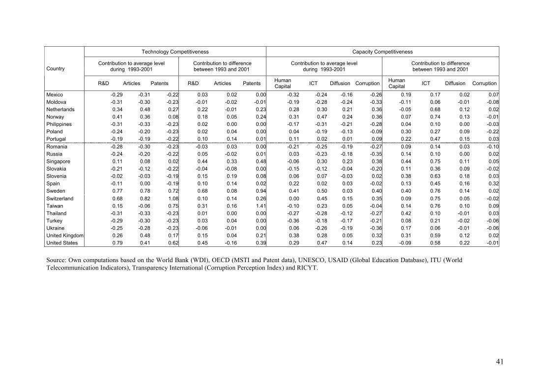
Table A3: Contribution of Sub-components to the Composite Indicators

Technology Competitiveness Capacity Competitiveness

Contribution to average level during 1993-2001

Contribution to difference between 1993 and 2001

Contribution to average level during 1993-2001

Contribution to difference between 1993 and 2001 Country

R&D Articles Patents R&D Articles Patents Human Capital ICT Diffusion Corruption Human

Capital ICT Diffusion Corruption

Argentina -0.26 -0.27 -0.22 0.01 0.04 0.00 -0.04 -0.20 -0.11 -0.21 0.30 0.21 -0.01 -0.16Austria 0.27 0.17 0.16 0.32 0.15 0.25 0.12 0.21 0.17 0.21 0.08 0.60 0.13 0.07Belarus -0.28 -0.27 -0.23 0.01 0.00 0.01 0.02 -0.23 -0.19 -0.17 0.08 0.08 -0.01 0.15Belgium 0.29 0.22 0.18 0.34 0.13 0.28 0.43 0.19 0.14 0.06 0.11 0.46 0.11 0.11Brazil -0.24 -0.31 -0.23 0.04 0.02 0.00 -0.30 -0.24 -0.17 -0.24 0.51 0.19 0.04 0.13Bulgaria -0.28 -0.21 -0.23 -0.04 -0.08 0.00 -0.06 -0.16 -0.21 -0.23 0.23 0.16 0.04 0.19Canada 0.28 0.49 0.45 0.28 -0.16 0.37 0.32 0.31 0.12 0.38 -0.24 0.48 0.19 -0.01Chile -0.26 -0.27 -0.22 0.02 0.00 0.00 -0.18 -0.18 -0.12 0.16 0.15 0.29 0.07 0.05China -0.29 -0.33 -0.23 0.04 0.01 0.00 -0.43 -0.30 -0.19 -0.30 0.09 0.12 0.06 0.13Croatia -0.23 -0.20 -0.22 0.05 0.02 0.01 -0.15 -0.12 -0.15 -0.22 0.05 0.30 0.10 0.18Czech Rep. -0.12 -0.10 -0.21 0.09 0.01 0.01 -0.13 -0.06 -0.01 -0.08 0.11 0.51 0.09 -0.22Denmark 0.41 0.58 0.25 0.47 0.10 0.40 0.26 0.45 0.12 0.45 0.22 0.73 0.18 0.00Estonia -0.25 -0.13 -0.22 0.08 0.14 0.01 0.06 -0.04 -0.11 0.01 0.29 0.40 0.11 -0.04Finland 0.52 0.56 0.51 0.69 0.23 0.65 0.41 0.38 0.05 0.42 0.22 0.60 0.18 0.08France 0.39 0.21 0.21 0.13 0.09 0.14 0.17 0.21 0.05 0.14 0.02 0.51 0.10 -0.03Germany 0.45 0.19 0.54 0.24 0.11 0.40 0.09 0.24 0.12 0.27 0.02 0.64 0.06 -0.10Greece -0.21 -0.10 -0.22 0.10 0.10 0.01 0.08 0.03 -0.06 -0.09 0.23 0.43 0.12 -0.05Hong Kong -0.20 -0.02 -0.08 0.13 0.20 0.17 -0.21 0.31 0.22 0.20 0.01 0.69 0.08 0.12Hungary -0.21 -0.12 -0.19 0.05 0.07 0.00 -0.06 -0.10 -0.08 -0.08 0.23 0.40 0.14 0.05Indonesia -0.32 -0.34 -0.23 0.00 0.00 0.00 -0.44 -0.33 -0.20 -0.37 0.12 0.03 0.02 -0.06Ireland 0.06 0.04 -0.06 0.30 0.13 0.17 0.12 0.20 1.24 0.29 0.04 0.65 2.36 -0.17Israel 0.58 0.72 0.54 0.95 -0.21 0.72 0.02 0.17 0.02 0.20 0.17 0.58 0.05 -0.07Italy 0.01 0.01 -0.04 0.07 0.10 0.06 0.04 0.12 0.03 -0.16 0.11 0.53 0.09 0.23Japan 0.65 0.10 1.39 0.27 0.10 0.63 0.07 0.22 0.20 0.11 0.09 0.59 0.05 0.04Korea 0.14 -0.20 0.14 0.35 0.20 0.44 0.20 0.11 0.06 -0.13 0.28 0.52 0.11 -0.03Latvia -0.29 -0.26 -0.22 0.02 -0.01 0.00 -0.02 -0.13 -0.17 -0.25 0.40 0.30 0.10 0.16Lithuania -0.27 -0.27 -0.23 0.05 0.04 0.01 -0.05 -0.16 -0.15 -0.12 0.33 0.22 0.03 0.22Malaysia -0.29 -0.32 -0.22 0.04 0.01 0.01 -0.33 -0.16 -0.06 -0.04 0.25 0.27 0.04 -0.03

40

Technology Competitiveness Capacity Competitiveness

Contribution to average level during 1993-2001

Contribution to difference between 1993 and 2001

Contribution to average level during 1993-2001

Contribution to difference between 1993 and 2001 Country

R&D Articles Patents R&D Articles Patents Human Capital ICT Diffusion Corruption Human

Capital ICT Diffusion Corruption

Mexico -0.29 -0.31 -0.22 0.03 0.02 0.00 -0.32 -0.24 -0.16 -0.26 0.19 0.17 0.02 0.07Moldova -0.31 -0.30 -0.23 -0.01 -0.02 -0.01 -0.19 -0.28 -0.24 -0.33 -0.11 0.06 -0.01 -0.08Netherlands 0.34 0.48 0.27 0.22 -0.01 0.23 0.28 0.30 0.21 0.36 -0.05 0.68 0.12 0.02Norway 0.41 0.36 0.08 0.18 0.05 0.24 0.31 0.47 0.24 0.36 0.07 0.74 0.13 -0.01Philippines -0.31 -0.33 -0.23 0.02 0.00 0.00 -0.17 -0.31 -0.21 -0.28 0.04 0.10 0.00 -0.03Poland -0.24 -0.20 -0.23 0.02 0.04 0.00 0.04 -0.19 -0.13 -0.09 0.30 0.27 0.09 -0.22Portugal -0.19 -0.19 -0.22 0.10 0.14 0.01 0.11 0.02 0.01 0.09 0.22 0.47 0.15 0.03Romania -0.28 -0.30 -0.23 -0.03 0.03 0.00 -0.21 -0.25 -0.19 -0.27 0.09 0.14 0.03 -0.10Russia -0.24 -0.20 -0.22 0.05 -0.02 0.01 0.03 -0.23 -0.18 -0.35 0.14 0.10 0.00 0.02Singapore 0.11 0.08 0.02 0.44 0.33 0.48 -0.06 0.30 0.23 0.38 0.44 0.75 0.11 0.05Slovakia -0.21 -0.12 -0.22 -0.04 -0.08 0.00 -0.15 -0.12 -0.04 -0.20 0.11 0.36 0.09 -0.02Slovenia -0.02 -0.03 -0.19 0.15 0.19 0.08 0.06 0.07 -0.03 0.02 0.38 0.63 0.18 0.03Spain -0.11 0.00 -0.19 0.10 0.14 0.02 0.22 0.02 0.03 -0.02 0.13 0.45 0.16 0.32Sweden 0.77 0.78 0.72 0.68 0.08 0.94 0.41 0.50 0.03 0.40 0.40 0.76 0.14 0.02Switzerland 0.68 0.82 1.08 0.10 0.14 0.26 0.00 0.45 0.15 0.35 0.09 0.75 0.05 -0.02Taiwan 0.15 -0.06 0.75 0.31 0.16 1.41 -0.10 0.23 0.05 -0.04 0.14 0.76 0.10 0.09Thailand -0.31 -0.33 -0.23 0.01 0.00 0.00 -0.27 -0.28 -0.12 -0.27 0.42 0.10 -0.01 0.03Turkey -0.29 -0.30 -0.23 0.03 0.04 0.00 -0.36 -0.18 -0.17 -0.21 0.08 0.21 -0.02 -0.06Ukraine -0.25 -0.28 -0.23 -0.06 -0.01 0.00 0.06 -0.26 -0.19 -0.36 0.17 0.06 -0.01 -0.06United Kingdom 0.26 0.48 0.17 0.15 0.04 0.21 0.38 0.28 0.05 0.32 0.31 0.59 0.12 0.02United States 0.79 0.41 0.62 0.45 -0.16 0.39 0.29 0.47 0.14 0.23 -0.09 0.58 0.22 -0.01

Source: Own computations based on the World Bank (WDI), OECD (MSTI and Patent data), UNESCO, USAID (Global Education Database), ITU (World Telecommunication Indicators), Transparency International (Corruption Perception Index) and RICYT.

41