The Compensating Differentials Model

Christopher Taber

September 20, 2015

Outline

Supply of Workers to Jobs

Firm Side

Hedonic Price Model

Applications

Roback

Bergstrom

Compensating Differentials

(or equalizing differences)

In the Roy model people only cared about income, but differedin skills

In the simplest version of this model people

Have identical skillsHeterogeneity in tastes for jobs

Basic idea is that an employer must pay a premium to get youto do some job you don’t want to do

Let D represent a disamenity of work like how dangerous it is

Suppose

D = 0 represents safe jobs that pay W0

D = 1 represents dangerous jobs that pay W1

All safe jobs will pay the same because workers are identicaland labor market is competitive (and frictionless)

Preferences

Ui(C,D)

C0 = I + W0

C1 = I + W1

where I is nonlabor income

Compensating difference is determined by indifferent individual

Lets figure out what the supply curve looks like

Take a really simple case with linear utility so that

Ui(C,D) = C − δiD

Then individual i chooses to work in dangerous sector if

Ui(C0,0) < Ui(C1,1)

I + W0 < I + W1 − δi

δi < W1 − W0 ≡ ∆W

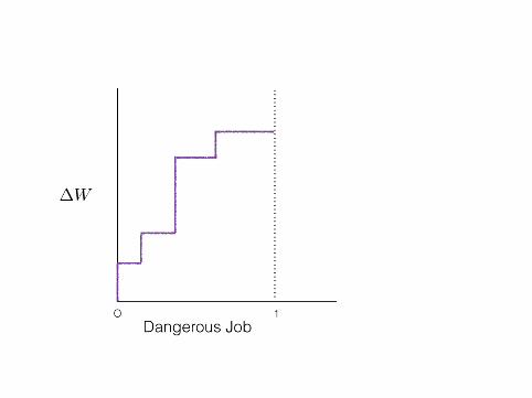
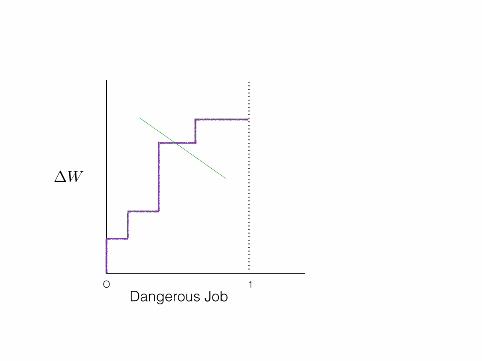
For person i the supply curve looks like:

Now suppose that δi varies over the population with measure G

Let 1(•) be the indicator function

Supply of people to dangerous jobs can be written as

Ns1 (∆W ) =

∫1 (δi < ∆W ) dG(δi)

= G (∆W )

Similarly supply to safe jobs is just

Ns0 (∆W ) = 1 − G(∆W )

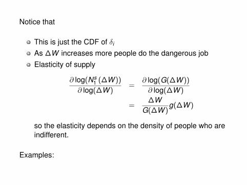
Notice that

This is just the CDF of δi

As ∆W increases more people do the dangerous jobElasticity of supply

∂ log(Ns1 (∆W ))

∂ log(∆W )=

∂ log(G(∆W ))

∂ log(∆W )

=∆W

G(∆W )g(∆W )

so the elasticity depends on the density of people who areindifferent.

Examples:

Firm Side

Now lets think about the firm side of the market

It costs money to make the workplace safe

The cost varies across jobs (this is easier for a university than acoal mine)

Each firm (job) hires one worker and there are as many firmsas workers

Production for the firm j is Fj

Costs of making the work environment safe is βj

so profits as a function of working environment is

Fj − βj (1 − D) − WD

Thus the workplace is dangerous if

W1 < W0 + βj

βj > ∆W

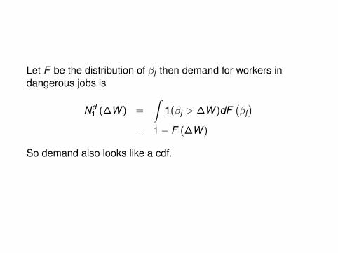
Let F be the distribution of βj then demand for workers indangerous jobs is

Nd1 (∆W ) =

∫1(βj > ∆W )dF

(βj)

= 1 − F (∆W )

So demand also looks like a cdf.

Putting them together

Hedonic Price Model

More generally suppose that danger is continuous

Let W (D) be the wage paid at mortality rate D

Worker chooses D to maximize

U i(I + W (D),D)

soU i

cW ′ = −U iD

Firm minimizes costs of production

W (D) + β j(D)

soW ′ = −β j′

I am not going to get into detail (See Rosen)

Applications

Occupational ChoiceImmigration/MigrationEnvironmentLocal public financeIndustry wage differencesHuman capital/SignalingLabor Supply

Roback (JPE, 1982)Jobs located in different cities

Measure value of local amenities

Workers and Firms choose where to locate

Depends on:

Rent in each placeWage rates in each place

To keep things simple I will assume that workers are identical inskills and tastes

Generalizing this so they are just perfect substitutes would bestraight forward

Moving costs between places is zero

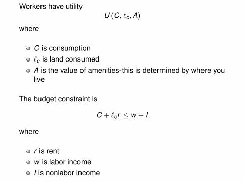
Workers have utilityU (C, `c ,A)

where

C is consumption`c is land consumedA is the value of amenities-this is determined by where youlive

The budget constraint is

C + `cr ≤ w + I

where

r is rentw is labor incomeI is nonlabor income

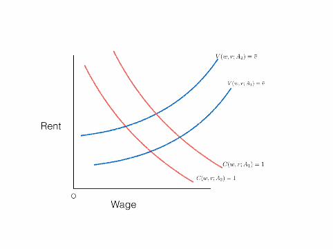
Let V (w , r ; A) be the associated indirect utility function with

∂V (w , r ; A)

∂w≥ 0

∂V (w , r ; A)

∂r≤ 0

∂V (w , r ; A)

∂A≥ 0

Since all individuals have to be indifferent between living indifferent locations, there is a value v such that

V (w , r ; A) = v

Production

Firms production function depends on land, the number ofworkers, and potentially the Amenity

X = F (`p,N; A)

where

`p is land used in productionN is the number of workersX is goods produced which have price oneF is constant returns to scale

Let C(w , r ; A) be the unit cost function

We allow free entry so in equilibrium

C(w , r ; A) = 1

where

∂C(w , r ; A)

∂w=

NX> 0

∂C(w , r ; A)

∂r=

`pX> 0

The sign of ∂C(w ,r ;A)∂A is indeterminate depending on the

particular amenity

Ocean, ∂C(w ,r ;A)∂A < 0

Public Schools, ∂C(w ,r ;A)∂A = 0

Regulations on Clean Air, ∂C(w ,r ;A)∂A > 0

Lets consider two cities with

A2 > A1

Think about 4 different cases:

∂V (w ,r ;A)∂A > 0, ∂C(w ,r ;A)

∂A = 0In this case the trade off between w and r is the same inboth cities for the firms∂V (w ,r ;A)

∂A = 0, ∂C(w ,r ;A)∂A > 0

∂V (w ,r ;A)∂A > 0, ∂C(w ,r ;A)

∂A > 0∂V (w ,r ;A)

∂A > 0, ∂C(w ,r ;A)∂A < 0

Lets think about equilibrium over a large number of cities

We know that

C(w , r ; A) = 1V (W , r ; A) = v

So

dVdA

= Vw∂w∂A

+ Vr∂r∂A

+ VA = 0

dCdA

= Cw∂w∂A

+ Cr∂r∂A

+ CA = 0

Substituting for ∂r∂Aand solving for ∂w

∂A gives

CwVw∂w∂A

+ CwVr∂r∂A

+ CwVA = 0

−VwCw∂w∂A

− VwCr∂r∂A

− VwCA = 0

∂w∂A

=Vr CA − Cr VA

Cr Vw − Vr Cw∂r∂A

=VwCA − CwVA

CwVr − VwCr

Thus ifCA = 0 ∂w

∂A < 0 ∂r∂A > 0

CA > 0 ∂w∂A < 0 ∂r

∂A??

CA < 0 ∂w∂A ?? ∂r

∂A > 0

Lets think about implementing this model empirically

We want to measure how tastes for cities vary

We can observe how wages and rental rates vary across cities

We can use these to measure “revealed preference” foramenities

We know that

Cw =NX

Cr =`pX

− Vr

Vw= `c

The shadow price of the amenity can be defined as

P∗A ≡ VA

Vw

=−Vw

∂w∂A − Vr

∂r∂A

Vw

= −∂w∂A

+ `c∂r∂A

The worth to the firm

CA = −Cw∂w∂A

− Cr∂r∂A

= −NX∂w∂A

−`pX∂r∂A

From the point of view of policy, the total value of the amenitycan be written as:

NP∗A − CAX = N[−∂w∂A

+ `c∂r∂A

]+ −N

∂w∂A

+ `p∂r∂A

= [N`c + `p]∂r∂A

Roback implements this to gauge the value of life in each city

One problem is that we are assuming that worker quality andhousing quality is the same across regions

She relaxes this by assuming that workers are perfectsubstitutes

Worker i in city j earns

Eij = wjLi

and

log(Eij) = log(wj) + log(Li)

= Z ′j γ + uj + X ′i β + ui

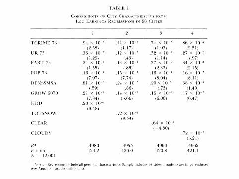
I .\BI.F. 1

O ' F I I I 0 1 H l 1 S FRO11 Lo(. F..\KYIs(;\ K~( .KTSSION\ I N 98 (:I rlF\

1 2 3 4

T( :RIRl t 13 .94 x 1 0 F . 4 4 x lo-" .74 x 1 0 - 7 8 6 x 10 -j (2.58) (1.17) ( I .93) (2.21)

L-K 73 .36 x 10-' . I 2 x lo-' .32 x lo-' . 2 i x lo-' 11.29) (.4:1) (1.14) ( . 9 i )

P . \RT 73 .24 x .13 x 10r3 .37 x lo-3 .34 x 1 0 ~ (1..5.5) ( 3 6 ) (2.33) 12.15)

P O P 79 ,113 x .15 x lo-' . 1 6 x lo-' . 1 6 x l o 7 (7.97) (7.74) (8.04) (8.11)

DE.SSSSIS.1 .81 x 10-"24 x 10-"20 x lo-;' .38 x I O F ( ,29) (.86) (.73) (1.40)

(;KO\V 6070 . 2 1 ~ 1 0 - ~ . 1 4 x 1 0 - ' . l 5 x I O - ' . 1 7 x 1 0 - ' 17.84) (.5.66) (6.06) (6.47)

HDD .20 x lo-" (8.48)

-I-O.I-SN()\V .72 x 10r3 (3.54)

(:I2F,.1R . 6 4 X 10-' (-4.80)

C;l.OC D l - .72 x lO-' 15.21)

R 2 ,4980 ,4955 ,4960 ,4962 F-~.;~rio 421.2 420.0 420.8 421.1 .\' = 12.001

TvLLges associated with high unemployment. Population size and the population growth rate both have the expected strong positive effects \I hile population density (DENSSMSX) is consistently insignificant.

T h e climate variables in table 1 perform I-emai-kably well. Heating degree days (HDD), total sno~vfall (TOTSNOW), and the number- of cloudy davs (C;LXILTDY) all have strong positive coefficients, which suggests that these indicators of climate are net disamenities. T h e nun~ber-of cleai- days (CLEAR) has a strongly negative coefficient, ~vhich is consistent with the prior notion that clear- days are arnenii- hle.'"

T h e nest question to be addressed is: What is the influence of the tit!- attributes o n the lvell-kno\vn regional differences in earnings! These persistent region efkcts have al~vays been something of a puzzle because a mobile labor force ought to bid auray anv geographic differences in real ear-nings. Because "real earnings" should be defined broadly to mean utility, we test the hypothesis that the ob-

',' P O Iothel- ~ e s u l t s on climate, see Hoch (1977).

--

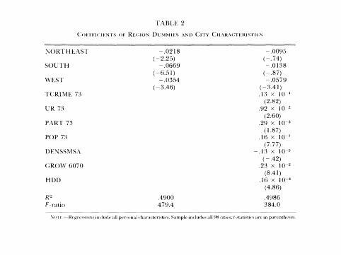
( , O l . k k I ( ItX-I\ I l k Rk:(;lOY DL\1 \1 lP- \ AYr) ( : 1 1 ! <:H \R.A<'l t R I S I I ( . \

-

S O K T H t..\S 1 . 0 2 18 - .0095 (-2.25) (p .74 )

SOL-I'H , 0 6 6 9 -.01:18 (-6.51) (p .87 )

\VEST -.OS.i4 -.0579 (-3.46) (-3.41)

TCRI\IF. 73 . I 0 x 10 (2.82)

LR 73 .92 x 10V2 12.60)

P . \ K I 7:3 .29 x lo-" ( 1.87)

POP 73 , I 6 x 10-i 17.77)

L)ESSS\lS;\ . 1 3 x 10-5 ( p . 4 2 )

(;RO\V 6070 .2:3 x lo-2 (8.41 )

HDD .16 x 10 -' (4.86)

R' .4!)00 ,4986 F-~.,\tio 479.4 984.0

served earnings differentials are in f'act proxies for different amenity levels. T h e first column oftable 2 presents evidence of the existence of regional effects in these data.16 T h e t-statistics on all three of the regional durnmies indicate significant differences in wages across regiotls. Furthermore, an F-test of joint significance of these three variables (compa1-ing eq. 1 of table 2 with the equation in the Xppen- dix) gives an F-value of 14.87 \vhere the critical F-value is 1.88.

\Ye expect that the inclusion of various measures of city attractive- ness may considerably dirninish the effect of region per se. =\ corn-parison of columns 1 and 2 oftable 2 gives some support for this idea. T h e coefficients on the northeastern and southern durnrnies fall dramatically, and the t-statistics indicate no difference in wages be- tTveen these t~vo regions and the hfidn.est. 'I'he persistent strength of the Mrestern effect is the only anornaly in this pattern. I t is certainly c o l ~ e c tto infer from these results that earnings are lo~ver in the \Vest than elsewhere. However, once differences in amenities are taken into :iccount, region plays a g1-eatly reduced role in explaining earnings. The fact that l o ~ c wages in the \Vest are accompanied 11y extremely

'"or- lut thet e \ i d e ~ l r e of and debate about the effect ot region, see Coelho and (;h;tli ( 197 1 ) and I . ,~denson(19'73).

1 ] 2 - ' > ] O L 7 R S . \ l . O F P O I I'I.I(::\L~ F( O \ - O \ l YA

P 4 R I 73

POP 77

1)E \5S>154

(TKO\\ 6070

HDD

high growth rates of population suggests that living in the Ll'est may t)e a proxy for some unmeasured desirable clirnatic o r cultural attri- butes. 'I'hus, the combined evidence seems persuasive that the re- gional differences in earnings can be largely accounted for t)y re-gional differences in local amenities."

2. Implicit PI-ices and Quality of Life Indices

Table 3 presents the results of a series of land price equations compa- ral~le to those in table 1 . The only significant results are the positive coefficients on the unemployment rate, population density, and population gro~vth. 'I'he latter t~vo results are most likely demand effects, ~vliich PI-osy for some unmeasured attributes o f t h e city. 'I'he theory suggests that the land price gradient reveals the rnarginal social value of the amenity to the community. '[he reader may be

" T h i \ result is ~.ot)ust to the inclusion of rnrasul-e\ of cost of living ( \ r e Rohack 1980).

tempted to inf'ei- from the zero coefficients on crime and pollution that these conditions have no social disutility. T h e limitations of' the data discussed earlier rnake such a conclusion premature. 'locompute the implicit price of each attribute in percentage terms,

\ve need the coefficients horn tables 1 and 3, as well as the budget shai-e of' land. 'I'his budget shai-e Jvas computed from the FHA data by multiplying the fi-action of' income spent on the mortgage (approxi- mately 17.8 percent) by the ratio of' the site pi-ice to the total value of' the house (approximately 19.6percent). 'I'his number was then aver- aged over a11 83 FHA cities to yield an average budget share. 'I'able 4 repoi-ts the irnplicit pi-ices computed from the columns of tables 1 and 3. For example, colurnn 2 reports the pi-ices computed from regres- sions, which include total annual snowfall as the climate variable. .A negative nurnl~ei- indicates a "bad" ~vhile a positive number indicates a good. [Vhile rrlost of the variables perform as expected, looking across the ~ . o ~ v s of' table 4 reveals some sensitivity of' the prices to specifica- t1011.

Each entrv in table 4 tells the marginal price of' the amenity evalu- ated at average annual earnings. Foi- example, the average person

I.(:KI\lE. 73 ~cl . imrsiI00 popul,trion)

YR 73 i f 1-dctiotl U I I C . I I I ~ ~ ~ \ C ~ )

P .IR I' 73 ~ ~ i ~ i c r ~ ~ g ~ ~ , t t ~ ~ \ i c ~ ~ O i cI I I C . ~ C . I )

POP 7:i ( 10.000 pc~l-\oll\)

DENSS\IS.I I 100 per-ion\'\cluarr ~iiile)

C;RO\V 6050 (per( rnt,rgc (hang? in popul;t- tion)

Hr)r) ( 1' I; coltlr.r tot- one t l ,~ \

I - o l - s N o \ V (iticties)

(:Lt:.iK (( l ' l \ \ )

(:I.( )YI)Y ( t I ' t \ \ )

0

2c

35

3p

3

ra 2

.FF

2 5

g.

q

23

-3

=Cw4

"2 :.?w 3

< 'T w -

w2 3

,;

22 ?

.%

22

1

CD

wTS??

ran

ia"

2 '

2 G

2

Cra

??

2"

2;

"&

5%

-2 2

3z

3 4

2R2

,7i

.m ,

3

2.

3 <

CL,

.$ f "

,,?

-4g

.9 5

w

3 50

52

-

0

3;$

FE

E.

w

~8.:

E 2

m+.

C";

SF-

2 2 r

a 2.

2.

3 E

2. c

.5

2 2.72

.-

3 3

5.

-. s

;.g

TW

4-. K

, g 5.T

'a c.

2 2

6.

mC

-T

Is

3g

23

CD

n

3

'-r+

.0cm

'5X3

f

2c

s??

-z2

3gw

-?m

3r

a

Bergstrom, Soldiers of Fortune

In Essays in Honor of K.J. Arrow, 1986.

Basic idea might not have been original to Bergstrom, but itdemonstrates it nicely

Everyone in our country is identical (ex-ante)

We need π fraction of the population to be in the army

The rest (1 − π) are farmers

How do we get people to enter the army?

Volunteer (compensating differential)Draft

Let w be per capita GDP

Thus it must be the case that

πCA + (1 − π) CF = πWA + (1 − π) WF = w

where

Cj is consumption in job jWj is wage at job j

Let

uA(CA) be utility from consumption if in armyuF (CF ) be utility from consumption if a farmer

uA (c) < uF (c)

U ′′A < 0,U ′′F < 0

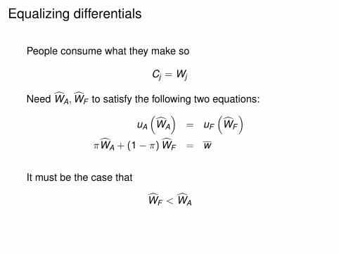
Equalizing differentials

People consume what they make so

Cj = Wj

Need WA, WF to satisfy the following two equations:

uA

(WA

)= uF

(WF

)πWA + (1 − π) WF = w

It must be the case that

WF < WA

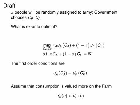
Draftπ people will be randomly assigned to army; Governmentchooses CF ,CA

What is ex-ante optimal?

maxCA,CF

πAuA (CA) + (1 − π) uF (CF )

s.t. πCA + (1 − π) CF = w

The first order conditions are

u′A (C∗A) = u′F (C∗F )

Assume that consumption is valued more on the Farm

u′A (c) < u′F (c)

But this implies thatCF > CA

This result is the opposite of compensating differentials

A feasible solution to the problem is to set CF = WF andCA = WA

Thus ex-ante utility of agents is higher with draft

Compensating differentials seems to be inefficient becauselevels of utility are equated rather than marginal utility

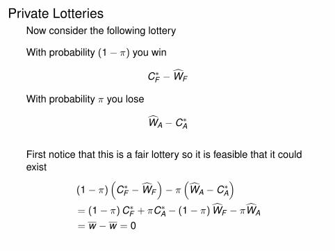
Private LotteriesNow consider the following lottery

With probability (1 − π) you win

C∗F − WF

With probability π you lose

WA − C∗A

First notice that this is a fair lottery so it is feasible that it couldexist

(1 − π)(

C∗F − WF

)− π

(WA − C∗A

)= (1 − π) C∗F + πC∗A − (1 − π) WF − πWA

= w − w = 0

What occupation do winners and losers choose?

First recall thatuA

(WA

)= uF

(WF

)and since

u′A (c) = u′F (c)

everywhere then it must be the case that for ∆ > 0

uA

(WA + ∆

)< uF

(WF + ∆

)and

uA

(WA − ∆

)> uF

(WF − ∆

)

Now if I win I get

uA

(WA + C∗F − WF

)Army

uF

(WF + C∗F − WF

)= uF

(C∗F)

Farmer

Since C∗F − WF is positive I will choose to be a farmer.

If I lose I get

uA

(WA −

(WA − C∗A

))= uA

(C∗A)

Army

uF

(WF −

(WA − C∗A

))Farmer

Since WA − C∗A is positive I will choose to enter the army.

Thus

This is a fair gambleIt is self-regulating:

winners choose to be farmerslosers choose to enter army

Gives the optimal ex-ante utility so workers would chooseto enter these lotteries