the comeback of inflation as an optimal public finance … comeback of inﬂation as an optimal...

The Comeback of Inflation as an OptimalPublic Finance Tool∗

Giovanni Di Bartolomeo,a Patrizio Tirelli,b andNicola Acocellac

aDepartment of Economics and Law, Sapienza University of RomebDEMS, University of Milan Bicocca

cMEMOTEF, Sapienza University of Rome

We challenge the widely held belief that New Keynesianmodels cannot predict optimal positive inflation rates. In fact,interest rates are justified by the Phelps argument that mone-tary financing can alleviate the burden of distortionary tax-ation. We obtain this result because, in contrast with pre-vious contributions, our model accounts for public transfersas a component of fiscal outlays. We also contradict the viewthat the Ramsey policy should minimize inflation volatilityand induce near-random-walk dynamics of public debt in thelong run. In our model it should instead stabilize debt-to-GDPratios in order to mitigate steady-state distortions. Our resultsthus provide theoretical support to policy-oriented analyseswhich call for a reversal of debt accumulated in the aftermathof the 2008 financial crisis.

JEL Codes: E52, E58, J51, E24.

1. Introduction

Optimal monetary policy analyses (Khan, King, and Wolman 2003;Schmitt-Grohe and Uribe, SGU henceforth, 2004a) identify two key

∗The authors are grateful to the IJCB editor Pierpaolo Benigno, three anony-mous referees, Fabio Canova, Martin Ellison, Jordi Galı, Luca Onorante, PaoloPaesani, Paul Levine, Frank Smets, and seminar participants at EC2 2011 Confer-ence (EUI), MMF2012 (Trinity College, Dublin), National Bank of Poland, andUniversities of Milan Bicocca, Cork, and Crete for useful comments on earlierdrafts. The authors acknowledge financial support from MIUR (PRIN). PatrizioTirelli also gratefully acknowledges financial support from EC project 320278 -RASTANEWS.

43

44 International Journal of Central Banking January 2015

frictions driving the optimal level of long-run (or trend) inflation.The first one is the adjustment cost of goods prices, which invari-ably drives the optimal inflation rate to zero. The second one ismonetary transaction costs that arise unless the central bank imple-ments the Friedman rule, i.e., a zero nominal inflation rate in steadystate. In their survey of the literature, SGU (2011) argue that theoptimality of zero inflation is robust to other frictions, such as nom-inal wage adjustment costs, downward wage rigidity, hedonic prices,the existence of an untaxed informal sector, and the zero bound onthe nominal interest rate. This latter result is broadly confirmed byCoibion, Gorodnichenko, and Wieland (2012), who find that theoptimal inflation rate is low, typically less than 2 percent, evenwhen the economy is hit by costly but infrequent episodes at thezero lower bound. A consensus therefore seems to exist that mone-tary transaction costs are relatively small at zero inflation, and thatimplementing low and stable inflation is the proper policy.

This theoretical result is in sharp contrast with empirical evi-dence. For instance, both in the United States and in the euro area,average inflation rates over the 1970–99 period have been close to5 percent. Even the widespread central bank practice of adoptinginflation targets between 2 percent and 4 percent is apparently atodds with theories of the optimal inflation rate (SGU 2011).

Furthermore, following the buildup of large stocks of debt inthe aftermath of the 2007–8 financial crisis, some economists haveargued that the public debt surge should be reversed and that atemporary increase in inflation might be necessary to achieve thisgoal. For instance, Rogoff (2010) suggests that “two or three yearsof slightly elevated inflation strikes me as the best of many verybad options.” Blanchard, Dell’Ariccia, and Mauro (2010) point atthe potential role of the inflation tax as one among several distor-tionary taxes which are available to policymakers. Aizenman andMarion (2011) predict that a 6 percent inflation rate would reducethe debt-to-GDP ratio by 20 percent within four years. These con-tributions are in line with the well-known Phelps (1973) argumentthat to alleviate the burden of distortionary taxation, it might beoptimal for governments to resort to monetary financing, driving awedge between the private and the social cost of money.

The Phelps argument has been widely investigated in the frame-work of general equilibrium models, and never found sufficient to

Vol. 11 No. 1 The Comeback of Inflation 45

warrant the optimality of a significantly positive inflation rate. Twomain results have been established. The first one is that distortionarytaxation does not warrant deviations from the Friedman rule unlessfactor incomes are sub-optimally taxed (see SGU 2011 and referencescited therein). The underlying intuition is that since all resourcesare eventually used for consumption, then the inflation tax, whichaffects consumption transaction costs, is desirable only to the extentthat other taxes have a sub-optimal effect on consumption. The sec-ond main result is that when the goods market characterization ismodified to account for (sub-optimally taxed) monopolistic distor-tions, numerical simulations suggest that the optimal inflation rateis negative and very close to zero, even accounting for the Phelpseffect (SGU 2004a). This conclusion carries over to the optimalityof near-zero volatility of inflation and near-random-walk behavior ingovernment debt and tax rates in response to shocks, implying thatthe recent increase of public debt in developed economies shouldbe regarded as a tax-smoothing device in response to the financialcrisis.

Our paper reconsiders the importance of the Phelps effect andobtains results that challenge the optimality of near-zero inflationrates when the tax system is incomplete. We show that a non-negligible inflation rate might indeed be optimal and that inflation(and tax rates) volatility should be exploited in order to stabilizedebt-to-GDP ratios in the long run.

The starting point in our analysis is that the optimal zero-inflation result obtained in dynamic stochastic general equilibrium(DSGE) models with incomplete tax systems is the consequence ofunrealistic assumptions about the size and composition of publicexpenditure. In the literature, standard calibrations of public expen-ditures focus on public-consumption-to-GDP ratios, typically set at20 percent (SGU 2004a; Aruoba and Schorfeide 2011). This follows along-standing tradition in business-cycle models, where only publicconsumption decisions have real effects. In our framework this choiceis not correct, because the focus here is on distortionary financing ofpublic expenditures in steady state, where also other components ofpublic expenditure matter. To the best of our knowledge, the onlyexception is SGU (2006), who determine the optimal inflation ratein a medium-scale model where public consumption and transfersrespectively amount to about 20 percent and 9 percent of GDP.


They find that the optimal inflation rate is positive but very small,half a percentage point, and that the inclusion of public transfersaccounts for a 0.7 percent increase in the optimal inflation rate.Their intuition for the inflationary effect of public transfers is thatonly transfers are pure rents to households and inflation is an indirecttax on those pure rents.

As a matter of fact, public consumption accounts for a limitedcomponent of the overall public expenditures in OECD countries,and transfers are relatively large (table 1).

We show that just allowing for a plausible parameterizationof public consumption and transfers in the SGU (2004a) modelreverses the standard conclusion about the optimal inflation rate,which now monotonically increases from 2 percent to 12 percentas the transfers-to-GDP ratio goes from 10 percent to 20 percent.Further, our calculations contradict the claim that public trans-fers per se require an inflation tax (SGU 2006). In fact, we alsofind that, absent public transfers, very large public-consumption-to-GDP ratios are also associated with a positive inflation rate. Forinstance, we obtain that the optimal inflation rate monotonicallyincreases from 2 percent to 12 percent as the public-consumption-to-GDP ratio grows from 40 percent to 47 percent. Given the his-torically observed public consumption ratios, these latter resultsare not empirically relevant, but they challenge received wisdomabout the reasons why level and composition of public expendi-tures should matter for the identification of the optimal inflationrate.

By working with a simplified version of our model, we are ableto show that changes in public consumption and public transferswould generate identical variations in the optimal inflation rateif public consumption did not affect the aggregate resource con-straint. The limited incentive to inflate that we observe in responseto a public consumption variation is due to its contemporaneouseffects that operate through the aggregate resource constraint andimpact on (i) inflation- and labor-tax revenues, and (ii) the plan-ner’s desired marginal rate of substitution between consumption andleisure.

We also investigate the optimal fiscal and monetary policyresponses to shocks. The issue is admittedly not new, but we areable to provide new contributions to the literature. When prices are


Table 1. Government Expenditures and Revenues,1998–2008 (average ratios to GDP)

Public Other Public TotalConsumption Expenditures Revenues

Australia 18.00 16.97 36.26Austria 19.10 32.29 49.71Belgium 22.13 27.82 49.39Canada 19.49 21.56 42.08Czech Republic 21.24 22.81 40.12Denmark 25.84 27.88 55.96Finland 21.75 27.74 53.12France 23.39 29.21 49.90Germany 18.96 27.58 44.61Greece 16.52 28.32 40.19Hungary 21.98 27.42 43.20Ireland 15.11 19.40 44.16Italy 19.10 28.94 45.25Japan 17.07 21.28 31.81Netherlands 23.57 22.19 45.34New Zealand 17.97 20.89 42.01Norway 20.76 23.54 56.63Poland 17.95 25.34 39.20Portugal 19.57 25.48 41.59Slovak Republic 20.24 21.35 36.55Spain 17.75 21.52 38.67Sweden 26.67 29.03 57.21Switzerland 11.4 23.48 34.40United Kingdom 19.83 22.28 40.38United States 15.26 20.51 33.47Euro Area 20.17 27.11 45.39

Source: OECD.

flexible and governments issue non-contingent nominal debt (Chari,Christiano, and Kehoe 1991), it is optimal to use inflation as alump-sum tax on nominal wealth, and the highly volatile inflationrate allows to smooth taxes over the business cycle. This result isintuitive insofar as taxes are distortionary whereas inflation volatilityis costless. SGU (2004a) show that when price adjustment is costly,


optimal inflation volatility is in fact minimal and long-run debtadjustment allows to obtain tax smoothing over the business cycle.In our paper, the SGU result is reversed, even when the amount ofpublic transfers is relatively small (12 percent of GDP). In this case,tax and inflation volatility are exploited to limit debt adjustment inthe long run.

The interpretation of our result is simple. As discussed above,public transfers increase the tax burden in steady state. In thiscase, the accumulation of debt in the face of an adverse shock—which would work as a tax-smoothing device in SGU (2004a)—is lessdesirable, because it would further increase long-run distortions. Toavoid such distortions, the policymaker is induced to front-load fiscaladjustment and to inflate away part of the real value of outstandingnominal debt. Consumption smoothing is therefore reduced relativeto SGU (2004a).

To the best of our knowledge, this is the first study of theoptimal interaction between inflation and tax policies when trans-fers account for the relatively large proportion of public expendi-tures that is documented in the data. A number of recent papershave analyzed the macroeconomic implications of public transferschemes, but their focus is different from ours. Alonso-Ortiz andRogerson (2010) investigate the labor supply response and the wel-fare implications of an optimal public transfer scheme in the con-text of a model with idiosyncratic productivity shocks, incompletefinancial markets, and flexible prices. Oh and Reis (2011) analyzethe role of transfers for consumption stabilization in the context ofheterogeneous agents, incomplete markets, and sticky prices—whentaxes are lump sum, no public debt accumulation is allowed andthe central bank is constrained to implement a zero-inflation pol-icy. Angelopoulos, Philippopoulos, and Vassilatos (2009) maintainthe representative-agent hypothesis and incorporate an uncoordi-nated redistributive struggle for transfers into an otherwise standardDSGE model. Zubairy (2014) investigates the consequences of tem-porary public transfer shocks in an estimated representative-agentDSGE model.

The remainder of the paper is organized as follows. The nextsection describes the model. Section 3 introduces the Ramsey pol-icy and illustrates our main results. Section 4 discusses optimalmonetary and fiscal stabilization policies. Section 5 concludes.


2. The Model

We consider a simple infinite-horizon production economy populatedby a continuum of households and firms whose total measures arenormalized to one. Monopolistic competition and nominal rigidi-ties characterize product markets. The labor market is competitive.A demand for money is motivated by assuming that money facil-itates transactions. The government finances an exogenous streamof expenditures by levying distortionary labor income taxes and byprinting money. Optimal policy is set according to a Ramsey plan.

As discussed by SGU (2011), positive inflation may be a desir-able instrument if some part of income is sub-optimally taxed. Inthe narrow framework of our model, the choice of inflating the econ-omy depends on untaxed monopolistic profits in the goods mar-ket, and the introduction of a uniform income tax would reduce theincentive to inflate. However, the tax system might be incompleteor sub-optimal for other reasons. For instance, one might take intoaccount the existence of an informal sector of the economy, or intro-duce monopolistic competition in the labor market. Here the modelis deliberately simple to highlight the theoretical challenge to theclaim that price stability is indeed optimal even when the tax sys-tem is incomplete. Providing a complete quantitative analysis of theoptimal inflation rate is beyond the scope of the paper.

2.1 Households

The representative household (i) maximizes the following utilityfunction:

U = Et=0

∞∑t=0

βtu (ct,i, lt,i) ;

u (ct,i, lt,i) = ln ct,i + η ln (1 − lt,i) , (1)

where β ∈ (0, 1) is the intertemporal discount rate, ct,i =(∫ 10 ct,i(j)

ρdj) 1

ρ

is a consumption bundle, and lt,i denotes theindividual labor supply. The consumption price index is Pt =(∫ 1

0 pt(j)ρ

ρ−1 di) ρ−1

ρ

.


The flow budget constraint in period t is given by

ct,i (1 + s(vt,i)) +Mt,i

Pt+

Bt,i

Pt= (1 − τt) wt,ilt,i +

Mt−1,i

Pt

+ θt +Rt−1Bt−1,i

Pt+ tt, (2)

where wt,i is the real wage; τt is the labor income tax rate; tt denotesreal fiscal transfers; θt is firms’ profits; Rt is the gross nominal inter-est rate; and Bt,i is a nominally riskless bond that pays one unit ofcurrency in period t + 1. Mt,i defines nominal money holdings to beused in period t + 1 in order to facilitate consumption purchases.

Consumption purchases are subject to a transaction cost1

s(vt,i), s′(vt,i) > 0 for vt,i > v∗, (3)

where vt,i = Pt,ict,i

Mt,iis the household’s consumption-based money

velocity. The features of s(vt,i) are such that a satiation level ofmoney velocity (v∗ > 0) exists where the transaction cost vanishesand, simultaneously, a finite demand for money is associated with azero nominal interest rate. Following SGU (2004a) the transactioncost is parameterized as2

s(vt,i) = Avt,i +B

vt,i− 2

√AB. (4)

The first-order conditions of the household’s maximization prob-lem are3

ct(j) = ct

(pt(j)Pt

) 1ρ−1

(5)

1See Sims (1994), SGU (2004a, 2011), Guerron-Quintana (2009), and Altiget al. (2011).

2Our results are robust to the alternative specification for the transactioncost used by Brock (1989) and Kimbrough (2006), which implies a Cagan (1956)money demand function. A proof is available upon request. The model is alsocompatible with Baumol (1952) demand for money (see SGU 2004a).

3When solving its optimization problem, the household takes as given goodsand bond prices. As usual, we also assume that the household is subject to asolvency constraint that prevents it from engaging in Ponzi schemes.


λt =uc (ct, lt)

1 + s(vt) + vts′(vt)(6)

λt = βEt

(λt+1Rt

πt+1

)(7)

λt (1 − τt) wt = −ul (ct, lt) (8)

Rt − 1Rt

= s′(vt)v2t . (9)

Equation (5) is the demand for the good j. As in SGU (2004a),condition (6) states that the transaction cost introduces a wedgebetween the marginal utility of consumption and the marginal util-ity of wealth that vanishes only if v = v∗. Equation (7) is a standardEuler condition where πt+1 = Pt+1/Pt denotes the gross inflationrate. Equation (8) defines the individual labor supply condition.Finally, equation (9) implicitly defines the money demand function,such that

Mt

Pt=

(Rt − 1RtA

+B

A

)− 12

ct. (10)

2.2 Firms’ Pricing Decisions

Each firm (j) produces a differentiated good:4

yt(j) = ztlt,j , (11)

where zt denotes a productivity shock.5

We assume a sticky-price specification based on Rotemberg(1982) quadratic cost of nominal price adjustment:

ξp

2yt (πt − 1)2 , (12)

4We abstract from capital accumulation and assume constant returns to scaleof employed labor. The consequences of these two assumptions are discussed inSGU (2006) and SGU (2011), respectively. Our results are not affected by theintroduction of diminishing returns to scale for labor (simulation results availableupon request).

5We assume that ln zt follows an AR(1) process.


where ξp > 0 is a measure of price stickiness. In line with Ascari,Castelnuovo, and Rossi (2011), we assume that the reoptimizationcost is proportional to output.6

In a symmetrical equilibrium, the price adjustment rule satisfies

zt (ρ − mct)1 − ρ

+ ξpπt (πt − 1) = Etβyt+1λt+1

ytλtξp [πt+1 (πt+1 − 1)] ,

(13)

where

mct =1zt

wt. (14)

From (5) it would be straightforward to show that 1ρ = μp defines

the price markup that obtains under flexible prices.

2.3 Government Budget and Aggregate Resource Constraints

The government supplies an exogenous, stochastic, and unproduc-tive amount of public good gt and implements exogenous trans-fers tt. Government financing is obtained through a labor incometax, money creation, and issuance of one-period, nominally risk-freebonds. The government’s flow budget constraint is then given by7

Rt−1bt−1 + gt + tt = τtwtlt +Mt − Mt−1

Pt+ bt, (15)

where bt = Bt

Ptdefines real debt.

The aggregate resource constraint closes the model:

yt = ct (1 + s(vt)) + gt +ξp

2yt (πt − 1)2 . (16)

6Our results are independent of this assumption. A proof is available uponrequest.

7As in SGU (2004a), ln(gt/yt), is assumed to evolve exogenously following anindependent AR(1) process. We assume instead that the level of the real transfer(tt/yt) is non-stochastic.


3. Ramsey Policy

3.1 Optimal Fiscal and Monetary Policy

The Ramsey policy is a set of plans {ct, lt, λt, mct, πt, vt, Rt, τt, bt}+∞t=0

that maximizes the expected value of (1) subject to the competitiveequilibrium conditions (6), (7), (8), (9), (11), (13), (14), (15), and(16), and to the exogenous fiscal and technology shocks. Given (6),(8), and (14), labor-tax revenues may be written as

τtwtlt =(

ztmct +ul (ct, lt) (1 + s(vt) + vts

′(vt))uc (ct, lt)

)lt. (17)

Condition (17) simply states that government fiscal revenues areequivalent to the wedge between the firm’s wage cost and the house-hold’s desired wage rate.

The Lagrangian of the Ramsey planner problem can be writtenas follows:

L = E0

∞∑t=0

βt

{u (ct, lt) + λAR

t

[ztlt − ct (1 + st) − gt − ξpztlt (πt − 1)2

2

]

+ λBt

[λt − β

λt+1Rt

πt+1

]

+ λGBCt

[ct

vt+

Bt

Pt+

(ztmct +

ul (ct, lt) [1 + s(vt) + vts′(vt)]

uc (ct, lt)

)lt

− Rt−1Bt−1

Pt−1− ct−1

πtvt−1− gt − tt

]

+ λPht

[βyt+1λt+1ξpπt+1 (πt+1 − 1)

ytλt− zt (ρ − mct)

1 − ρ

− ξpπt (πt − 1)]

+ λMUCt

[uc (ct, lt)

1 + s(vt) + vts′(vt)− λt

]},

where R and s(v) are defined in (4) and (9), respectively.The solution requires numerical simulations.8 For the sake of

comparison, we calibrate our model as SGU (2004a). The time unit

8These are obtained implementing SGU (2004b) second-order approximationroutines.


is meant to be a year; the subjective discount rate β = 0.96 isconsistent with a steady-state real rate of return of 4 percent peryear. Transaction cost parameters A and B are set at 0.011 and0.075, the debt-to-GDP ratio is set at 0.44 percent, the benchmarklevel for the public-consumption-to-GDP ratio is 0.20, the gross pricemarkup is 1.2, and the annualized Rotemberg price adjustment costis 4.375 (this implies that firms change their price on average everynine months; see SGU 2004a, p. 210). The preference parameter η isset so that in the flexible-price steady state households allocate 20percent of their time to work when public transfers are nil.

In figure 1 we describe the steady-state optimal inflation responseto the transfer increase and to a corresponding variation in pub-lic consumption in addition to the benchmark 20 percent value.Both public consumption and transfers are defined as GDP ratios:gPC = gt/yt and gPT = tt/yt. Simulations show that steady-stateinflation rapidly increases when gPT grows beyond the 8 percentthreshold. For instance, the optimal inflation rate is close to 3 per-cent when gPT is 10 percent, and exceeds 12 percent when the trans-fer ratio is 20 percent. When public expenditure is confined to publicconsumption, a 40 percent public-consumption-to-GDP ratio is asso-ciated with a 2 percent optimal inflation rate, and optimal inflationmonotonically grows up to 12 percent as the public consumptionshare reaches 47 percent.9

Note that when different public consumption and transfers lev-els induce the Ramsey planner to choose identical inflation rates,we also obtain identical consumption, labor market, and inflationwedges, s(v), 1+s(v)+vs′(v)

(1−τ) , and ξp

2 l (π − 1)2 , respectively (figure 2).It is also interesting to note that when either gPT or gPC reach thelevels which trigger the optimality of positive inflation, the optimalpolicy generates an almost identical consumption pattern. In bothcases, abandoning price stability allows to stabilize consumption inspite of the increasing burden of fiscal revenues.

It is interesting to compare our results with the interpretation ofthe inflationary outcome generated by the need to finance transfersoffered by SGU (2006, p. 385). They claim that when the private

9As pointed out above, in our model untaxed monopolistic profits are nec-essary to generate the planner’s incentive to inflate. For instance, if one setsμp = 1.1, the optimal inflation rate remains close to zero for gPT ≤ 15 percent.


Figure 1. Public Expenditure Components and OptimalInflation

0 5 10 15 20-2

0

2

4

6

8

10

12

public transfers on output (%)

)%( noitalf ni

Panel (a)

20 30 40-2

0

2

4

6

8

10

12

public consumption on output (%)

Panel (b)

sector must receive an exogenous amount of after-tax transfers, itis optimal to exploit the inflation tax on money balances in orderto impose an indirect levy on the (transfers-determined) source ofhousehold income. Given our finding that relatively large levels ofpublic consumption exist such that the planner chooses identicalinflation rates, this intuition must be incorrect.

One mechanism driving the choice of the optimal policy mixmight be related to the distortionary taxation necessary to financethe additional transfers, which adversely affects the labor supplyand reduces the tax base, whereas the increase in public consump-tion generates a negative wealth effect that triggers a positive laborsupply response and expands the tax base. In this case, the incentiveto increase inflation should be much reduced. To check the impor-tance of the wealth effect of gPC on the labor supply, we solvedthe Ramsey problem under a different specification of the utilityfunction, such as the Greenwood-Hercowitz-Huffman (1988; GHHhenceforth) preferences,

GHHu (Ct,i, lt,i) =

(Ct,i − ηl1+φ

t,i

)1−σ

1 − σ. (18)


Fig

ure

2.Pol

icy

Wed

ges

and

Con

sum

ption

2030

40

0

0.1

0.2

0.3

0.4

publ

ic c

onsu

mpt

ion

on o

utpu

t

t soc t ne mt suj da

010

20

0

0.1

0.2

0.3

0.4 pu

blic

tra

nsfe

rs o

n ou

tput

t soc t ne mt suj da

2030

40-0

.010

0.01

0.02 pu

blic

con

sum

ptio

n on

out

put

egde w noi t p musnoc

010

20-0

.010

0.01

0.02 pu

blic

tra

nsfe

rs o

n ou

tput

egde w noi t p musnoc

2030

401234

publ

ic c

onsu

mpt

ion

on o

utpu

t

egde wr obal

020

12345 publ

ic t

rans

fers

on

outp

ut

egde wr obal

2030

400

0.050.

1

0.15 pu

blic

con

sum

ptio

n on

out

put

noi t p musnoc0

1020

0

0.050.

1

0.15 pu

blic

tra

nsfe

rs o

n ou

tput

noi t p musnoc

Not

es:T

hew

edge

sar

eco

mpu

ted

asfo

llow

s:P

rice

adju

stm

ent

cost

is(1

2).T

heco

nsum

ptio

nw

edge

is(4

).T

hela

bor

wed

geis

divi

ded

byλ.


Under (18) the marginal rate of substitution − ul(ct,lt)uc(ct,lt)

= ηlφt,i is inde-pendent of consumption, i.e., there is no wealth effect on the laborsupply, and the labor market equilibrium condition in steady state isηlφ = w. Simulations contradict our conjecture. In fact, under GHHpreferences we obtain almost identical inflation rates in response tothe variations in gPC and gPT considered in figure 1. In particular,an increase in public consumption is met by an expansion in thelabor tax, whereas inflation remains very close to zero unless publicconsumption is relatively large.10

3.2 The Ramsey Solution in a Simplified Model

Further insights can be obtained by imposing restrictions on someparameter values, which allow to simplify the Ramsey solution in thesteady state.11 To begin with, we set β = 1, ξp = 0. In this case, theFriedman rule is satisfied for π = 1 and price adjustment frictionsdo not matter, restricting the policymaker’s trade-off to two dimen-sions: the Friedman rule calls for complete price stability, whereasthe public finance motive calls for positive inflation because the taxsystem is incomplete. From (13) it is easy to see that in steady statew = ρ irrespective of the inflation rate. We also assume that steady-state debt is nil, and set B = 0 in (4). Under this latter assumption12

we obtain s(v) = Av and, since R = πβ , v =

(R−1AR

) 12 =

(π−1Aπ

) 12 .13

By setting gPC = 0.2 and gPT = 0, the optimal inflation rate inthe simplified model is π = 1.3 percent, whereas for the full modelwe obtained π = −0.16 percent. This result is obviously due to theassumed reduction in inflation costs, but our focus here is on obtain-ing a better understanding of the reason why similar levels of publictransfers and public consumption are associated with different opti-mal inflation rates in steady state. In this regard, note that a 5percent increase in gPC now is matched by π = 1.8 percent, whereasan identical variation in gPT is associated with π = 2.6 percent.

10Results are available upon request.11See the appendix for a derivation of our results.12With B = 0, the model is characterized by a standard Tobin money demand.13The result described in this section can also be obtained by removing the

assumptions ξp = B = 0, but in this case the algebra is rather cumbersome andit is more difficult to support the intuition.


In this simplified model, the steady-state Ramsey solution ischaracterized by λPh = λMUC = 0 and λB = −λGBC

tcvπ

1λ . This

latter condition implies that the marginal effect of inflation on theEuler equation constraint must equal the marginal effect of π on thegovernment budget constraint. Further, we obtain that the marginaleffect of money velocity on the aggregate resource constraint mustequal its marginal effect on the government budget constraint, i.e.,

λARcs′ (v) = λGBC[R′ (v)vπ2 − π − 1

v2π− 2δAl

1 − l

]c. (19)

Finally, the solution for λGBC is

λGBC = uc(c, l)[(

R′ (v)vπ2 − A − 2δAl

1 − l

)1 + s (v)

s′ (v)

+1v

π − 1π

− δlγ (v)1 − l

]−1

. (20)

The Ramsey planner’s choice of c takes into account effects on themarginal utility of consumption; on the aggregate resource con-straint, λAR [1 + s (v)] ; and on the government budget constraint,where 1

vπ−1

π and −δlγ(v)1−l define consumption effects on revenues

from inflation and from labor taxes, respectively. In a sense, justlike monetary transaction costs drive a wedge between the mar-ginal utility of consumption and the marginal utility of wealth inthe representative-household first-order condition (6), here mone-tary transaction costs and the need to enforce distortionary taxa-tion drive a wedge between the Ramsey planner’s marginal utilityof consumption and the marginal utility of revenues.

The optimal labor supply condition is

−uh(c, l) = λAR + λGBC

(ρ − δcγ (v)

(1 − l)2

)(21)

=

(R′ (v)Avπ2 − 1 − 2δl

1 − l+ ρ − δcγ (v)

(1 − l)2

)λGBC. (22)

The right-hand side of (21) accounts for the marginal effects of l onon the aggregate resource constraint (23), which is proportional to


the multiplier λAR, and on the government budget constraint (24),which is determined by the multiplier λGBC and by the marginaleffect of l on tax revenues,

(ρ − δcγ(v)

(1−l)2

). This is the Ramsey planner’s

equivalent of the representative-agent first-order condition (8).Using (19), (20), and the explicit functional forms for v , s (v),

and s′ (v) , the Ramsey planner’s problem collapses to the followingconditions:

c =1 − gPC

1 +(Aπ−1

π

) 12l (23)

c

lvπ − 1

π+

{ρ − δc

1 − l

[1 + 2

(A

π − 1π

) 12]}

= gPC + gPT (24)

δc

1 − l=

1−π2

π4 − δl1−l + ρ

2 − δc(

12 +

(Aπ−1

π

) 12)

/ (1 − l)2

(1−π2

π4 − δl1−l

)[1 +

(Aπ−1

π

) 12]

+ 12

(Aπ−1

π

) 12 −

δl

(12+(A π−1

π )12

)

1−l

.

(25)

Conditions (23) and (24), respectively, are the aggregate resourceand government balance constraints that the Ramsey planner solu-tion must satisfy. Condition (25) simply rearranges (21). It is easyto see that changes in gPC and gPT would generate identical vari-ations in consumption hours and inflation if public consumptiondid not enter the aggregate resource constraint (23). Therefore, thesmaller incentive to inflate that we observed in response to a pub-lic consumption variation is due to its contemporaneous effects thatoperate through the aggregate resource constraint and impact on (i)inflation- and labor-tax revenues, i.e., on the left-hand side of (24),and (ii) the planner’s desired marginal rate of substitution in (25).

In figure 3 we present a graphical solution. Substituting for cfrom (23) into (24), we obtain the GBC schedule which definescombinations of l and π that are consistent with a balanced gov-ernment budget constraint for given values of ρ, gPC , and gPT . It isupward sloping14 because an increase in employment can be obtainedthrough a labor-tax reduction. This, in turn, requires an increase in

14It is very steep for the small inflation range (1.00–1.10) used in figure 3.


Figure 3. Graphical Illustration of the RamseyEquilibrium

inflation in order to compensate for the revenue loss. By substituting(23) into (25), we obtain the MRS schedule which defines combina-tions of l and π such that the Ramsey planner’s desired marginal rateof substitution obtains for given values of ρ and gPC . It is downwardsloping15 because an increase in l brings the consumption-to-laborratio below its desired level. A fall in inflation is therefore necessaryto raise desired relative consumption. The MRS and GBC schedulesare plotted by assuming gPC = 0.2 and gPT = 0. The correspondingRamsey equilibrium is then point A.

Figure 4 describes the effects on the Ramsey equilibrium ofa 5 percent increase in public expenditure. Specifically, panel A

15Due to its complex functional form, the slope of (25) is not trivial. Note that,in addition to gPC , (25) includes only two calibrated parameters, A and δ, whichtake values 0.011 and 2.9 as in SGU (2004a). We experimented for values of Aand δ in the ranges 10−4–10 and 0.5–8, respectively. In all cases, we obtained adownward-sloping MRS schedule around realistic values for l and π (includingthe Ramsey equilibrium). Note that the different values for δ imply an equilib-rium for l between about 0.1 and 0.9. Therefore, we explored the range of allpossible values.


Figure 4. The Effects of a Change in GovernmentExpenditures

illustrates the effects of an increase in public transfers, whereas panelB shows the effects of an equivalent increase in public consumption.The common initial equilibrium in the two panels is described bypoint A, where gPC = 0.2 and gPT = 0.

Starting from point A in panel A, the 5 percent increase in gPT

shifts the GBC locus to the left to GBC′ because, holding infla-tion constant, the increase in the tax rate necessary to balance thebudget inevitably reduces employment. As pointed out above, theMRS schedule is not affected by gPT and the new equilibrium A′ ischaracterized by a relatively large increase in inflation.

The effects of a 5 percent increase in gPC , panel B, are morecomplex. Consider the GBC locus; in this case, for any given valueof l, private consumption must fall, causing a twofold effect on gov-ernment revenues. On the one hand, the reduction in real moneyholdings lowers inflation-tax proceedings. On the other hand, from(17) we know that for any given value of l, the lower private con-sumption is associated with larger fiscal revenues. This latter effectunambiguously dominates, limiting the leftward shift of GBC.16

16This latter effect also helps to explain why incentives to inflate remain limitedwhen the utility function is characterized by GHH preferences.


Turning to the MRS locus, we find that an increase in gPC nowalso causes a rightward shift to MRS′. This happens because forany given level of inflation, the planner seeks a reduction in leisureto partly offset the reduction in consumption determined by theincrease in gPC . Thus, relative to the increase in gPT , the shift inMRS would cause larger inflation, but this is dominated by thecorresponding shift in GBC.

4. Optimal Monetary and Fiscal Stabilization Policies

In this section we investigate whether our characterization of steady-state public expenditures also bears implications for the conduct ofmacroeconomic policies over the business cycle. SGU (2004a) showthat, when public transfers are nil, costly price adjustment inducesthe Ramsey planner to choose a minimal amount of inflation volatil-ity and to select a permanent public debt response to shocks inorder to smooth taxes over the business cycle. Benigno and Wood-ford (2004), who emphasize the complementarity between fiscal andmonetary policies, substantially confirm the optimality of near-zeroinflation volatility for a plausible degree of nominal price stickiness.

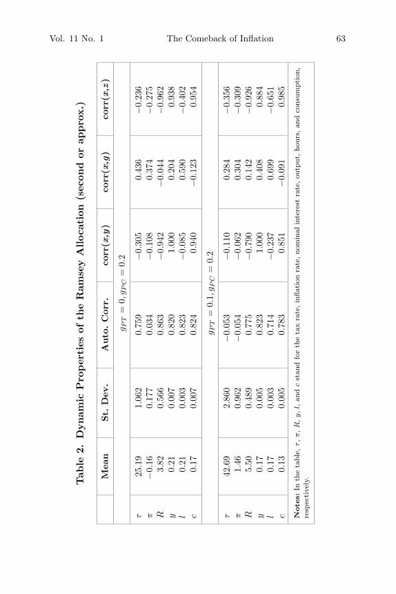
We discuss how the optimal fiscal and monetary stabilizationpolicies17 change when, in steady state, gPT is 0.1 instead of zero,whereas other fiscal figures are assumed to be 0.44 for debt-to-GDPratio and gPC = 0.2. In table 2 we show that the volatility of bothtaxes and inflation dramatically increases, whereas the strong per-sistence of taxes vanishes.18 Thus, even if we still obtain a unit rootin the dynamic process for debt accumulation, a more realistic cali-bration of fiscal outlays has important implications for the dynamicpattern of fiscal and monetary stabilization policies. To grasp thisintuition, consider the impulse response functions to a temporaryincrease in government purchases (figure 5).19

17We consider a productivity shock and a public consumption shock. Proper-ties of stochastic processes are described in table 2. We compute the second-orderapproximation using SGU (2004b) routines (see also SGU 2004a, section 7).

18To sharpen the analysis, we assume the shock is not serially correlated.19Additional experiments are reported in the working paper version of the

paper (downloadable from Ideas). Specifically, there we report the impulseresponse functions for different composition of the public expenditure and levelsof government debt.


Tab

le2.

Dynam

icP

roper

ties

ofth

eR

amse

yA

lloca

tion

(sec

ond

orap

pro

x.)

Mea

nSt.

Dev

.A

uto

.C

orr.

corr

(x,y

)co

rr(x

,g)

corr

(x,z

)

g PT

=0,

g PC

=0.

2

τ25

.19

1.06

20.

759

−0.

305

0.43

6−

0.23

6π

−0.

160.

177

0.03

4−

0.10

80.

374

−0.

275

R3.

820.

566

0.86

3−

0.94

2−

0.04

4−

0.96

2y

0.21

0.00

70.

820

1.00

00.

204

0.93

8l

0.21

0.00

30.

823

−0.

085

0.59

0−

0.40

2c

0.17

0.00

70.

824

0.94

0−

0.12

30.

954

g PT

=0.

1,g P

C=

0.2

τ42

.69

2.86

0−

0.05

3−

0.11

00.

284

−0.

356

π1.

460.

962

−0.

054

−0.

062

0.30

4−

0.30

9R

5.50

0.48

90.

775

−0.

790

0.14

2−

0.92

6y

0.17

0.00

50.

823

1.00

00.

408

0.88

4l

0.17

0.00

30.

714

−0.

237

0.69

9−

0.65

1c

0.13

0.00

50.

783

0.85

1−

0.09

10.

985

Note

s:In

the

tabl

e,τ,π,R

,y,l,

and

cst

and

for

the

tax

rate

,in

flati

onra

te,no

min

alin

tere

stra

te,ou

tput

,ho

urs,

and

cons

umpt

ion,

resp

ecti

vely

.


Figure 5. Fiscal Shock Impulse Response Functions underDifferent Levels of Public Transfers

0 2 4 6 8 100

0.5

1

1.5Debt

0 2 4 6 8 100

0.1

0.2Tau

0 2 4 6 8 100

0.02

0.04

0.06Nominal interest rate

0 2 4 6 8 100

0.05

0.1Inflation

0 2 4 6 8 10-0.2

-0.1

0Consumption

0 2 4 6 8 100

0.5

1Output

Notes: The solid line shows no transfers and the dashed line shows 10 percentof the transfers-to-GDP ratio. The figure shows impulse responses to an i.i.d.government purchases shock. The size of the innovation in government purchasesis one standard deviation (a 3 percent increase in g). The shock takes place inperiod 1. Public debt, consumption, and output are measured in percent devia-tions from their pre-shock levels. The tax rate, the nominal interest rate, and theinflation rate are measured in percentage points.

Under both scenarios, the permanent debt adjustment allows tosmooth tax distortions. However, the different magnitudes of thepermanent debt and tax adjustments associated with the two cases(gPT = 0 and gPT = 0.1) are also evident. When gPT = 0.1, thelong-run debt adjustment is reduced by 70 percent. In this case,long-run tax and inflation distortions are already relatively large,and the steady-state accumulation of debt in the face of an adverseshock becomes less desirable. Instead, the planner finds it optimal tofront-load tax adjustment and to inflate away part of the real value ofoutstanding nominal debt. In addition, the increase in inflation has


a positive impact on seigniorage revenues. This explains the surgein inflation volatility reported in table 2. Our model is also ableto match the positive empirical correlation between average infla-tion and inflation variability.20 For the sake of fairness, it is worthnoticing that inflation volatility still appears to be substantially lim-ited relative to the case of flexible prices, which is the main pointof SGU (2004a). Our contribution here is that a substantial com-plementarity exists between inflation and taxes in response to thepublic consumption shock.

5. Conclusions

Incompleteness of the tax system is a necessary condition for theexistence of a public finance justification for inflation. The strongpoint of SGU (2004a, 2011) was to argue that irrespective ofthe incompleteness of the tax system, optimal inflation should bebetween zero and the Friedman rule.

The point of this paper is that for the same incompleteness of thetax system, a non-negligible inflation rate in steady state is indeedoptimal if one adopts a realistic calibration for fiscal outlays, includ-ing public transfers. Differently from SGU (2011), who argue thatcentral bank inflation targets are too high, our contribution showsthat a 2 percent target might indeed be too low.

However, to obtain an empirically relevant assessment of the opti-mal inflation rate, the model should be extended to account for anumber of country-specific factors, such as governments’ ability tooptimally tax factor incomes, composition of public expenditures,monetary transaction costs, other frictions such as nominal wagestickiness, and the existence of an informal sector. All this shouldbe done bearing in mind that the tax system incompleteness prob-ably is an inherent feature of modern economies. Similar consider-ations can be made concerning inflation costs. For instance, Calvopricing, which implies price dispersion, might generate higher infla-tion costs than Rotemberg pricing, but one should also take intoaccount inflation indexation and its correlation with the underlying

20See, e.g., Friedman (1977), Ball and Cecchetti (1990), Caporale and McKier-nan (1997).


inflationary regime, as shown in Fernandez-Villaverde and Rubio-Ramırez (2008). All this is left for future research.

Further, our analysis of the optimal fiscal and monetary stabi-lization policies strengthens the Benigno and Woodford (2004) argu-ment that the two policy tools should be seen as complements andthat the monetary authority should consider the consequences oftheir actions for the government budget. In this regard, we showthat a substantial amount of inflation volatility is indeed desirableto deflate nominal debt and to limit the accumulation of real debt inthe long run. Our results thus provide theoretical support to policy-oriented analyses which call for a reversal of debt accumulated inthe aftermath of the 2008 financial crisis and for a reconsiderationof the role of inflation in facilitating debt reductions.

Appendix

The steady-state solution of the Ramsey problem defined in section3 is characterized by the following set of first-order conditions:

l = [1 + s(v)] c + gcl +ξp

2l(π − 1)2 (26)

1 = βr(v)1π

(27)

c

v+ b + [mc + Zγ(v)] l =

r(v)bπ

+c

vπ+ (gPC + gPT ) l (28)

ξp(1 − β)π(π − 1) =mc − ρ

1 − ρ(29)

uc(c, l) = λγ(v) (30)

uc(c, l) − λAR[1 + s(v)] +[

1v

(1 − β

π

)− δ

1 − llγ(v)

]λGBC

+ λMUCucc = 0 (31)

ul(c, l) + λAR

(1 − ξp

2(π − 1)2

)

+ λGBC

[mc −

(δc

1 − l+

δc

(1 − l)2l

)γ(v)

]= 0 (32)


(1 − r(v)

π

)λB + (1 − β)

λPh

λπ(π − 1) − λMUCγ(v) = 0 (33)

− λARs′(v)c − λB βr′(v)λπ

− λGBC[(

1 − β

π

)c

v2 +δc

1 − llγ′(v) +

βbr′(v)π

]

− λMUCλγ′(v) = 0 (34)

−λARξp(π − 1)l +1π2

[λBr(v)λ + λGBC

(r(v)b +

c

v

)]= 0 (35)

π = βr(v) (36)

ξpλGBCl = − λPh

1 − ρ, (37)

where we have expressed public consumption and transfers as GDPratio (i.e., g = gPC l and t = gPT l, recall that y = l) andr(v) = 1

1−s′(v)v2 from (9).As said in the main text, we impose β = 1, b = 0, ξp = 0,

and B = 0. In that case, v =(

R−1AR

) 12 =

(π−1Aπ

) 12 , s(v) = Av ,

s′(v) = A, and γ (v) = 1 + s(v) + vs′(v) = 1 + 2A12(

π−1π

) 12 .

From (37) we get λPh = 0. Then from equation (33) we getλMUC = 0. Equation (29) implies mc = ρ. From (35) we obtainλB λ

π = −[λGBC c

vπ2

].21 Then substitute λB λ

π = −λGBC cvπ2 into

(34) to obtain λAR = λGBC

s′(v)

[ρ′(v)vπ2 − A − 2δAl

1−l

]. Substituting for λAR

in (31), we obtain

λAR =Uc

s′(v)

[ρ′(v)vπ2 − A − 2δlA

1−l

]{[

ρ′(v)vπ2 − A − 2δlA

1−l

][1+s(v)]

s′(v) + 1v

(π−1

π

)− δl

1−lγ (v)} (38)

λs = uc(c, l){[

ρ′ (v)vπ2 − A − 2δlA

1 − l

][1 + s (v)]

s′ (v)

+1v

(π − 1

π

)− δl

1 − lγ (v)

}−1

. (39)

21This latter condition implies that the marginal effect of π on savings mustequal the marginal effect of π on the government budget constraint.


Then substituting for λGBC, λAR into (32), we get[2

π21

π2 − 1 − 2δl1−l

]+

{ρ − δcγ(v)

1−l − δcγ(v)l(1−l)2

}[

2π2

1π2 − 1 − 2δl

1−l

][1 + s (v)] + 1

v

(π−1

π

)− δl

1−lγ (v)=

c

1 − l. (40)

The model is then solved using (26), (28), and (40).

References

Aizenman, J., and N. Marion. 2011. “Using Inflation to Erode theU.S. Public Debt.” Journal of Macroeconomics 33 (4): 524–41.

Alonso-Ortiz, J., and R. Rogerson. 2010. “Taxes, Transfers andEmployment in an Incomplete Markets Model.” Journal of Mon-etary Economics 57 (8): 949–58.

Altig, D., L. Christiano, M. Eichenbaum, and J. Linde. 2011. “Firm-Specific Capital, Nominal Rigidities and the Business Cycle.”Review of Economic Dynamics 14 (2): 225–47.

Angelopoulos, K., A. Philippopoulos, and V. Vassilatos. 2009. “TheSocial Cost of Rent Seeking in Europe.” European Journal ofPolitical Economy 25 (3): 280–99.

Aruoba, S. B., and F. Schorfheide. 2011. “Sticky Prices versus Mon-etary Frictions: An Estimation of Policy Trade-Offs.” AmericanEconomic Journal: Macroeconomics 3 (1): 60–90.

Ascari, G., E. Castelnuovo, and L. Rossi. 2011. “Calvo vs. Rotem-berg in a Trend Inflation World: An Empirical Investigation.”Journal of Economic Dynamics and Control 35 (11): 1852–67.

Ball, L., and S. Cecchetti. 1990. “Inflation and Uncertainty at Shortand Long Horizons.” Brookings Papers on Economic Activity 1:215–54.

Baumol, W. J. 1952. “The Transactions Demand for Cash: An Inven-tory Theoretic Approach.” Quarterly Journal of Economics 66(4): 545–56.

Benigno, P., and M. Woodford. 2004. “Optimal Monetary and Fis-cal Policy: A Linear-Quadratic Approach.” In NBER Macroeco-nomics Annual 2003, ed. M. Gertler and K. Rogoff, 271–364.Cambridge, MA: MIT Press.

Blanchard, O. J., G. Dell’Ariccia, and P. Mauro. 2010. “RethinkingMacroeconomic Policy.” IMF Staff Position Note No. 2010/03.


Brock, P. L. 1989. “Reserve Requirements and the Inflation Tax.”Journal of Money, Credit and Banking 21 (1): 106–21.

Cagan, P. 1956. “The Monetary Dynamics of Hyperinflation.” InStudies in the Quantity Theory of Money, ed. M. Friedman,25–117. Chicago: University of Chicago Press.

Caporale, T., and B. McKiernan. 1997. “High and Variable Infla-tion: Further Evidence on the Friedman Hypothesis.” EconomicsLetters 54 (1): 65–68.

Chari, V., L. Christiano, and P. Kehoe. 1991. “Optimal Fiscaland Monetary Policy: Some Recent Results.” Journal of Money,Credit and Banking 23 (3): 519–39.

Coibion, O., Y. Gorodnichenko, and J. Wieland. 2012. “The Opti-mal Inflation Rate in New Keynesian Models: Should CentralBanks Raise Their Inflation Targets in Light of the Zero LowerBound?” Review of Economic Studies 79 (4): 1371–1406.

Fernandez-Villaverde, J., and J. Rubio-Ramırez. 2008. “How Struc-tural Are Structural Parameters?” In NBER MacroeconomicsAnnual 2007, ed. D. Acemoglu, K. Rogoff, and M. Woodford,83–137. Cambridge, MA: MIT Press.

Friedman, M. 1977. “Nobel Lecture: Inflation and Unemployment.”Journal of Political Economy 85 (3): 451–72.

Greenwood, J., Z. Hercowitz, and G. Huffman. 1988. “Investment,Capacity Utilization, and the Real Business Cycle.” AmericanEconomic Review 78 (3): 402–17.

Guerron-Quintana, P. A. 2009. “Money Demand Heterogeneity andthe Great Moderation.” Journal of Monetary Economics 56 (2):255–66.

Khan, A., R. G. King, and A. L. Wolman. 2003. “Optimal MonetaryPolicy.” Review of Economic Studies 70 (4): 825–60.

Kimbrough, K. P. 2006. “Revenue Maximizing Inflation.” Journalof Monetary Economics 53 (8): 1967–78.

Oh, H., and R. Reis. 2011. “Targeted Transfers and the FiscalResponse to the Great Recession.” NBER Working Paper No.16775.

Phelps, E. S. 1973. “Inflation in the Theory of Public Finance.”Swedish Journal of Economics 75 (1): 67–82.

Rogoff, K. S. 2010. “Why America Isn’t Working.” OnlineProject Syndicate Article. Available at http://www.project-syndicate.org/.


Rotemberg, J. J. 1982. “Sticky Prices in the United States.” Journalof Political Economy 90 (6): 1187–1211.

Schmitt-Grohe, S., and M. Uribe. 2004a. “Optimal Fiscal and Mon-etary Policy under Sticky Prices.” Journal of Economic Theory114 (2): 198–230.

———. 2004b. “Solving Dynamic General Equilibrium ModelsUsing a Second-Order Approximation to the Policy Function.”Journal of Economic Dynamics and Control 28 (4): 755–75.

———. 2006. “Optimal Fiscal and Monetary Policy in a Medium-Scale Macroeconomic Model.” In NBER Macroeconomics Annual2005, ed. M. Gertler and K. Rogoff, 383–425. Cambridge, MA:MIT Press.

———. 2011. “The Optimal Rate of Inflation.” In Handbook of Mon-etary Economics, ed. B. M. Friedman and M. Woodford, 723–828.Amsterdam: Elsevier.

Sims, C. A. 1994. “A Simple Model for Study of the Determinationof the Price Level and the Interaction of Monetary and FiscalPolicy.” Economic Theory 4 (3): 381–99.

Zubairy, S. 2014. “On Fiscal Multipliers: Estimates from a MediumScale DSGE Model.” International Economic Review 55 (1):169–95.

the comeback of inflation as an optimal public finance … comeback of inﬂation as an optimal...

Documents