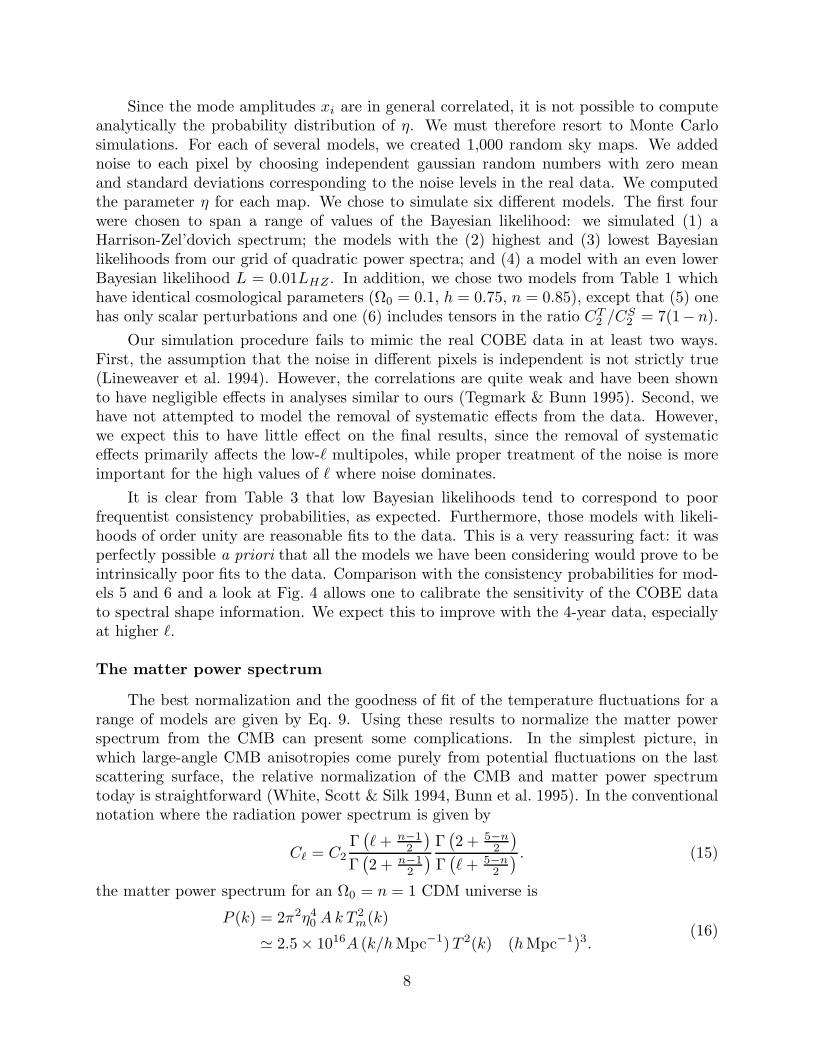
arX

iv:a

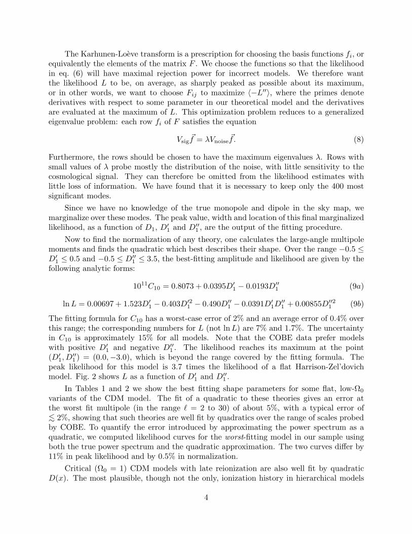
stro

-ph/

9503

054v

3 1

1 N

ov 1

995

CfPA-95-TH-02January 1995

Revised March 1995

The COBE Normalization of CMB Anisotropies

Martin White and Emory F. Bunn

Center for Particle Astrophysics, University of California,

Berkeley, CA 94720–7304

ABSTRACT

With the advent of the COBE detection of fluctuations in the Cosmic Microwave Back-ground radiation, the study of inhomogeneous cosmology has entered a new phase. It isnow possible to accurately normalize fluctuations on the largest observable scales, in thelinear regime. In this paper we present a model-independent method of normalizing theo-ries to the full COBE data. This technique allows an extremely wide range of theories tobe accurately normalized to COBE in a very simple and fast way. We give the best fittingnormalization and relative peak likelihoods for a range of spectral shapes, and discuss thenormalization for several popular theories. Additionally we present both Bayesian and fre-quentist measures of the goodness of fit of a representative range of theories to the COBEdata.

Subject headings: cosmic microwave background – methods: statistical

Introduction

Classically, it has been standard practice to normalize models of large-scale structureat a scale of ≃ 10 h−1Mpc, using a quantity related to the clustering of galaxies (herethe Hubble constant H0 = 100 h kms−1 Mpc−1) measured at the current epoch. Due toprocessing of the primordial spectrum and the large amplitude of the mass fluctuationswhich galaxies represent, this method of normalization requires assumptions about thehistory of the equation of state for matter inside the horizon, the non-linear evolution ofthe density field and the processes of galaxy formation. One of the key uncertainties isthe relationship between the observed structure and the underlying mass distribution inthe universe. With the COBE DMR detection of Cosmic Microwave Background (CMB)anisotropies (Smoot et al. 1992), it has become possible to directly normalize the potentialfluctuations at near-horizon scales, circumventing the problems with the ‘conventional’normalization.

In an earlier Letter we presented the normalization of the standard cold dark matter(CDM) model and a small range of variants (Bunn, Scott & White 1995). In this paperwe extend this to a larger class of models, and present a means for normalizing a wholeclass of models to the COBE data in a computationally simple manner. Throughout wewill use the 2-year COBE data (Bennett et al. 1994, Gorski et al. 1994, Wright et al. 1994,Banday et al. 1994, Gorski et al. 1995a) as released by NASA–GSFC. The normalization inthis data differs from that in the data used by the COBE group by ∼ 1µK (K.M. Gorski,private communication; Gorski et al., 1995b).

1

As discussed in Bunn et al. (1995) and Banday et al. (1994) there is more informationin the COBE data than just the RMS power measured. In other words, the COBE datacannot be reduced to a single number without a significant loss of information. One wayto see this is to notice that there are ∼ 90 eigenvalues of the signal-to-noise ratio witheigenvalue larger than 1. An alternative method is to note that the COBE data constrainsthe amplitude of the fluctuations over a range of scales, albeit a narrow range.

In Fig. 1 we show the RMS power in a model which is fittetedd to the COBE data withone free parameter. The toy model we have chosen is the so called Sachs-Wolfe spectrum(Sachs & Wolfe 1967) which assumes that the observed temperature fluctuations comepurely from the redshifts associated with climbing out of potentials on the last scatteringsurface (for a discussion see e.g. Peebles 1993; White, Scott & Silk 1994). Aside from thenormalization of the model (which is fixed by COBE) there is one free parameter: thespectral slope, denoted n, with n = 1 corresponding to a scale invariant spectrum. Wenotice that the total power is not constant, showing that the normalization to COBE issensitive to more than the total RMS fluctuations produced. Furthermore, the COBE datacontain information on the “shape” of the power spectrum, which means that some theoriesare more likely than others, given the data. We will now introduce a simple method forusing all of the information in the COBE data to normalize a wide class of models.

Model independent analysis

We have demonstrated that the COBE data contain more information than just thetotal power, which can be measured by 〈Q〉, σ(10), σ(7), band power, etc. However, itis still useful to have a method for normalizing a given model to the data, without havingto use the full sky maps containing 6144 pixels at 3 frequencies in each of two channels.We present here a method which allows one to normalize a large class of theories (thosewhich can be described by a power spectrum over the limited range of scales probed byCOBE) to the data in a simple manner.

To proceed we notice that theories with gaussian fluctuations (or fluctuations whichare gaussian on COBE scales) can be specified entirely in terms of a power spectrum.In CMB studies this is usually expressed as the variance of the multipole moments, as afunction of mode number, i.e. ℓ(ℓ + 1)Cℓ vs ℓ, where the temperature on the sky has beenexpanded in spherical harmonics

∆T

T(θ, φ) ≡

∑

ℓm

aℓmYℓm(θ, φ) (1)

and we define〈a∗

ℓmaℓ′m′〉 ≡ Cℓ δℓℓ′δmm′ (2)

For most theories the power spectrum is a smooth function. Following White (1994),we will write

D(x) = ℓ(ℓ + 1)Cℓ with x = log10 ℓ . (3)

We can perform a Taylor series expansion of D(x) about some fiducial point, which weshall take to be x = 1 (ℓ = 10). Many theories (see below) can be well approximated

2

by quadratic D(x) over the relevant range for COBE, roughly ℓ = 2 to 30, and so wepresent the normalizations and likelihoods of quadratic D(x). We choose to parameterizeour quadratics by the (normalized) first and second derivatives at x = 1: D′

1 and D′′

1 where

D(x) ≃ D1

(

1 + D′

1(x − 1) +D′′

1

2(x − 1)2

)

(4)

(note that D′

1 is 1/D1 times the derivative of D(x) at x = 1). The normalization is thengiven by quoting D1, or C10, for each (D′

1, D′′

1 ) pair, and the goodness of fit is quantifiedby the relative likelihood of that shape compared to a featureless, n = 1, Sachs-Wolfespectrum.

We compute the maximum-likelihood normalization for a grid of values of D′

1 andD′′

1 using the method described in Bunn & Sugiyama (1995) and Bunn et al. (1995). Wecombine the six publicly-available equatorial DMR sky maps pixel by pixel into a singlemap by performing a weighted average, with weights given by the inverse square of thenoise level in each pixel. (We obtain negligibly different results when the two 31 GHzmaps, which are more sensitive to Galactic contamination, are excluded. These maps havehigh noise levels, and are therefore automatically given low weights in the average.) Weexcise all pixels whose centers have Galactic latitude |b| < 20 from the map, leaving 4038pixels.

We then estimate the likelihood of getting this particular data set for each powerspectrum. Rather than computing the likelihood directly, which would involve repeatedinversions of a 4038×4038 matrix, we first perform a Karhunen-Loeve transform (Karhunen1947, Thierren 1992) to “compress” the data to a more manageable size. Specifically, wechoose a set of basis functions fi defined on the portion of the sphere outside of theGalactic cut. (The manner in which these functions are chosen is described below.) Wethen compute the inner product of the data vector with each of these functions:

xi =∑

j

fi(rj)∆T (rj), (5)

where rj is the position of the jth pixel, ∆T (rj) is the corresponding temperature fluc-tuation in the data, and the sum runs over all pixels. If we assume that the temperaturefluctuations are gaussian, then the projections xi will be gaussian as well. We can thereforecompute their likelihood in the usual way:

L ∝ (det V )−1/2

exp(

−12xiV

−1ij xj

)

, (6)

where Vij ≡ 〈xixj〉 is the covariance matrix, which contains contributions from the cosmicsignal and the noise:

V = Vsig + Vnoise = (FY )(BCB)(FY )T + FNFT , (7)

where Fij = fi(rj), Yiµ = Yℓm(ri), Cµν = Cℓδµν , B is the beam pattern, and Nij ≈ σ2i δij

is the covariance matrix of the noise in the sky map. (Here Greek indices stand for pairsof indices (ℓm), with µ = ℓ2 + ℓ + m + 1.)

3

The Karhunen-Loeve transform is a prescription for choosing the basis functions fi, orequivalently the elements of the matrix F . We choose the functions so that the likelihoodin eq. (6) will have maximal rejection power for incorrect models. We therefore wantthe likelihood L to be, on average, as sharply peaked as possible about its maximum,or in other words, we want to choose Fij to maximize 〈−L′′〉, where the primes denotederivatives with respect to some parameter in our theoretical model and the derivativesare evaluated at the maximum of L. This optimization problem reduces to a generalizedeigenvalue problem: each row fi of F satisfies the equation

Vsig~f = λVnoise

~f. (8)

Furthermore, the rows should be chosen to have the maximum eigenvalues λ. Rows withsmall values of λ probe mostly the distribution of the noise, with little sensitivity to thecosmological signal. They can therefore be omitted from the likelihood estimates withlittle loss of information. We have found that it is necessary to keep only the 400 mostsignificant modes.

Since we have no knowledge of the true monopole and dipole in the sky map, wemarginalize over these modes. The peak value, width and location of this final marginalizedlikelihood, as a function of D1, D′

1 and D′′

1 , are the output of the fitting procedure.

Now to find the normalization of any theory, one calculates the large-angle multipolemoments and finds the quadratic which best describes their shape. Over the range −0.5 ≤D′

1 ≤ 0.5 and −0.5 ≤ D′′

1 ≤ 3.5, the best-fitting amplitude and likelihood are given by thefollowing analytic forms:

1011C10 = 0.8073 + 0.0395D′

1 − 0.0193D′′

1 (9a)

lnL = 0.00697 + 1.523D′

1 − 0.403D′21 − 0.490D′′

1 − 0.0391D′

1D′′

1 + 0.00855D′′21 (9b)

The fitting formula for C10 has a worst-case error of 2% and an average error of 0.4% overthis range; the corresponding numbers for L (not lnL) are 7% and 1.7%. The uncertaintyin C10 is approximately 15% for all models. Note that the COBE data prefer modelswith positive D′

1 and negative D′′

1 . The likelihood reaches its maximum at the point(D′

1, D′′

1 ) = (0.0,−3.0), which is beyond the range covered by the fitting formula. Thepeak likelihood for this model is 3.7 times the likelihood of a flat Harrison-Zel’dovichmodel. Fig. 2 shows L as a function of D′

1 and D′′

1 .

In Tables 1 and 2 we show the best fitting shape parameters for some flat, low-Ω0

variants of the CDM model. The fit of a quadratic to these theories gives an error atthe worst fit multipole (in the range ℓ = 2 to 30) of about 5%, with a typical error of

∼< 2%, showing that such theories are well fit by quadratics over the range of scales probedby COBE. To quantify the error introduced by approximating the power spectrum as aquadratic, we computed likelihood curves for the worst-fitting model in our sample usingboth the true power spectrum and the quadratic approximation. The two curves differ by11% in peak likelihood and by 0.5% in normalization.

Critical (Ω0 = 1) CDM models with late reionization are also well fit by quadraticD(x). The most plausible, though not the only, ionization history in hierarchical models

4

of structure formation is standard recombination, followed by full ionization from someredshift z∗ until the present. The fully ionized phase is due (perhaps) to radiation frommassive stars on scales which go non-linear early. (See Liddle & Lyth 1995 for furtherdiscussion.) We find that, over the range of ℓ probed by COBE, models which have z∗ ∼< 100are almost indistinguishable from models with no reionization, assuming standard big-bangnucleosynthesis values for ΩB . There is of course damping on degree scales (ℓ ∼ 100), butlittle change in the spectrum at smaller ℓ. Further, the relative normalization of the matterand radiation power spectra is the same as in models with standard recombination. For aCDM model with h = 0.5 and n = 1, the quadratic parameters are well fit by the formulae

D′

1 = 0.738 − 0.0307z∗ + 3.32 × 10−4z2∗− 1.06 × 10−6z3

∗

D′′

1 = 1.554 − 0.0483z∗ + 3.67 × 10−4z2∗− 7.60 × 10−7z3

∗

(10)

over the range 30 ≤ z∗ ≤ 110.

The case of open CDM models is more complicated, since the Cℓ exhibit features atseveral scales. To add to the difficulty, there appear to be several different primordial spec-tra one can consider in open universe models. Some models based on inflationary phases(Lyth & Stewart 1990, Ratra & Peebles 1994, Bucher, et al. 1995) predict power spectrawhich show an increase in power near the curvature radius. All of these calculations makeuse of basis functions in which there is exponential damping of power above the curvatureradius; however, this assumption can be relaxed (Lyth & Woszczyna 1995, Yamamotoet al. 1995). For further discussion of these issues see the appendix. The open modelsof Ratra & Peebles (1994) have already been fitted to the 2-year COBE data (Gorski etal. 1995a) and we will not duplicate the results here. We mention, however, that the Cℓ

for such models can be fitted by cubics in log10 ℓ to the same accuracy that the ΛCDMmodels can be fitted by quadratics. This increases the dimension of the parameter spaceand makes tabulating the results more difficult. We defer consideration of cubic fits untilthe situation with regard to open models is more settled.

Once the 4-year COBE data becomes available, we hope a fitting formula similar toEq. 9 (but which goes to sufficiently high order to encompass almost all theories), could beproduced for the benefit of the astrophysics community. Such a fit, coded into a subroutine,would allow any theory to be quickly and accurately fitted to the COBE data. At presentour simple quadratic fit is sufficient for a wide range of theories of current interest.

The goodness of fit

Statistical methods for using a data set like COBE to place constraints on modelsgenerally come in two varieties, Bayesian and frequentist. Most CMB work, includinganalyses of the COBE data as well as other experiments, has taken a Bayesian point ofview. In the Bayesian approach, the probability of observing the actual data is computedfor each model. This may be denoted p(D|M), meaning “the probability of the data giventhe model”. One then assumes a “prior” probability distribution p(M) on the modelsand applies Bayes’s theorem to produce a “posterior” probability distribution giving thelikelihood p(M |D) of the various models given the data:

p(M |D) ∝ p(D|M)p(M). (11)

5

The posterior probability distribution tells us how likely each member of our family ofmodels is compared with any other member, which is what we would like to know.

The Bayesian approach is perfectly adequate for assessing the relative merits of thevarious models under consideration: with this approach we can say, for example, that modelA is 10 times more likely than model B. These models may only differ by a normalizationor could be drawn from different cosmologies or structure formation scenarios. In somecases however we would like to assign absolute consistency probabilities to models. TheBayesian approach is not well suited to answering this sort of question, and the problem ofassigning an absolute consistency probability to a model is best attacked with frequentistmethods.

In the frequentist approach, we choose some goodness-of-fit parameter η, and computeits probability distribution over a hypothetical ensemble of realizations of the model. Wethen compute the value of η corresponding to the real data, and determine the probabilityof finding a value of η as extreme as the observed value in a random member of ourensemble. We take this probability to be a measure of the consistency of the data withthe model: if the data does not occur often in realizations of the model, we say the modelis “unlikely” given the data.

Two points about this technique deserve emphasis. First, the consistency probabilitiesderived in this manner are conceptually quite distinct from Bayesian likelihoods. Bayesiansand frequentists ask different questions of their data, and will therefore sometimes getdifferent answers. We do expect that models which have low Bayesian likelihoods willin general have poor frequentist consistency probabilities; however, there is no generallyapplicable quantitative relation between the two. Second, it is clear that the success of thefrequentist approach depends on choosing an appropriate goodness-of-fit parameter η. Forsome classes of problems a standard choice is available; for the problem we consider below,we are unaware of such a standard. This is because the measurement of CMB fluctuationsinvolves detecting extra noise on the sky. Thus the correlation function, or errors on thetemperatures, which are used in the fit depend on the theory being tested, unlike normallyexamined cases of model fitting.

We wish to assign frequentist consistency probabilities to various power spectra. Thefirst goodness-of-fit parameter one might think of for this purpose is a simple χ2,

χ2 ≡M∑

i=1

(

xi

σi

)2

, (12)

where xi is the amplitude of the ith element in our eigenmode expansion, σ2i is the variance

predicted for xi by our model, and M is the number of modes in the expansion. (Inorder to remove all sensitivity to the monopole and dipole, the eigenmodes fi should beorthogonalized with respect to these modes before the xi are computed.) This parameterwould be a natural choice if we wished to constrain the normalization of a model; however,our primary interest is in constraining the shape of the power spectrum, and this goodness-of-fit parameter is not well suited for this purpose. In fact, given any power spectrumCℓ, we can choose a normalization that gives a χ2 that lies exactly at the median of its

6

probability distribution, since σi scales with the normalization of the theory. We wouldtherefore conclude that for some normalization this model is a perfectly good fit regardlessof the shape of the Cℓ.

To focus on the power spectrum, let us consider quantities quadratic in the amplitudeof the eigenmodes. There is a complication due to the presence of the galaxy in the COBEmaps, which breaks the rotational symmetry of the COBE sky. This makes it difficult todefine a rotationally symmetric quantity (like Cℓ) by summing over azimuthal variable m.However, this is only a technical complication and we can still define a measure of powerby binning the squares of the mode amplitudes in bins that probe particular angular scales.We expand each eigenmode fi in spherical harmonics and compute an “effective ℓ” probedby that mode by performing a weighted average over ℓ with weights given by the squaresof the coefficients of the expansion. (The modes are generally quite narrow in ℓ-space, sothe results are not sensitive to the exact method of computing the effective ℓ.) We thensort the modes in order of increasing effective ℓ (decreasing angular scale). As it happens,the result of this procedure is almost identical to sorting the modes in order of decreasingsignal-to-noise eigenvalue. We then compute the quantities

zi =iK∑

j=(i−1)K+1

(

xj

σj

)2

(13)

for 1 ≤ i ≤ M/K. We should choose the bin size K to be large enough to reduce theintrinsic width of the distribution of zi to a reasonable level, yet small enough that themode amplitudes in each bin probe similar angular scales. We have adopted K = 10 as acompromise between these two considerations.

If our model is correct, then each zi will be approximately K. If the model is incorrect,then some zi will be too low, and others will be too high. For example, if our model hastoo little large-scale power, then the variances xj/σj will be greater than 1 for small j,and the first few zi will tend to be larger than K. We can quantify this observation bydefining the goodness-of-fit parameter

η =

M/K∑

i=1

(zi − K)2. (14)

The zi for a Harrison-Zel’dovich spectrum and our worst-fitting model (model 4 ofTable 3) are shown in Fig. 3. (In making Fig. 3 we chose the coarser bin size K = 20rather than K = 10, to reduce scatter in the points.) Note that with our definition thezi only loosely correspond to Cℓ and depend on the theory. When zi is larger than itsexpected value, one can conclude that the data have more power than the theory on thecorresponding angular scale; however, there is no direct proportionality between zi andthe corresponding Cℓ. Each zi can be regarded as an estimator of the power spectrumof the signal and noise combined. For small i, zi samples mostly signal, while the noisedominates for large i. The value of zi for large i therefore changes very little as the modelparameters are varied, as can be seen in Fig. 3.

7

Since the mode amplitudes xi are in general correlated, it is not possible to computeanalytically the probability distribution of η. We must therefore resort to Monte Carlosimulations. For each of several models, we created 1,000 random sky maps. We addednoise to each pixel by choosing independent gaussian random numbers with zero meanand standard deviations corresponding to the noise levels in the real data. We computedthe parameter η for each map. We chose to simulate six different models. The first fourwere chosen to span a range of values of the Bayesian likelihood: we simulated (1) aHarrison-Zel’dovich spectrum; the models with the (2) highest and (3) lowest Bayesianlikelihoods from our grid of quadratic power spectra; and (4) a model with an even lowerBayesian likelihood L = 0.01LHZ . In addition, we chose two models from Table 1 whichhave identical cosmological parameters (Ω0 = 0.1, h = 0.75, n = 0.85), except that (5) onehas only scalar perturbations and one (6) includes tensors in the ratio CT

2 /CS2 = 7(1− n).

Our simulation procedure fails to mimic the real COBE data in at least two ways.First, the assumption that the noise in different pixels is independent is not strictly true(Lineweaver et al. 1994). However, the correlations are quite weak and have been shownto have negligible effects in analyses similar to ours (Tegmark & Bunn 1995). Second, wehave not attempted to model the removal of systematic effects from the data. However,we expect this to have little effect on the final results, since the removal of systematiceffects primarily affects the low-ℓ multipoles, while proper treatment of the noise is moreimportant for the high values of ℓ where noise dominates.

It is clear from Table 3 that low Bayesian likelihoods tend to correspond to poorfrequentist consistency probabilities, as expected. Furthermore, those models with likeli-hoods of order unity are reasonable fits to the data. This is a very reassuring fact: it wasperfectly possible a priori that all the models we have been considering would prove to beintrinsically poor fits to the data. Comparison with the consistency probabilities for mod-els 5 and 6 and a look at Fig. 4 allows one to calibrate the sensitivity of the COBE datato spectral shape information. We expect this to improve with the 4-year data, especiallyat higher ℓ.

The matter power spectrum

The best normalization and the goodness of fit of the temperature fluctuations for arange of models are given by Eq. 9. Using these results to normalize the matter powerspectrum from the CMB can present some complications. In the simplest picture, inwhich large-angle CMB anisotropies come purely from potential fluctuations on the lastscattering surface, the relative normalization of the CMB and matter power spectrumtoday is straightforward (White, Scott & Silk 1994, Bunn et al. 1995). In the conventionalnotation where the radiation power spectrum is given by

Cℓ = C2

Γ(

ℓ + n−12

)

Γ(

2 + n−12

)

Γ(

2 + 5−n2

)

Γ(

ℓ + 5−n2

) . (15)

the matter power spectrum for an Ω0 = n = 1 CDM universe is

P (k) = 2π2η40 A k T 2

m(k)

≃ 2.5 × 1016A (k/hMpc−1) T 2(k) (h Mpc−1)3.(16)

8

with A = 3C2/(4π). In models such as CDM this relation works quite well, as long asmatter-radiation equality is sufficiently early (h is not too low). Even for h = 0.3 therelation works at the 4% level and if h = 1 the error is ∼< 1%. See Bunn et al. (1995) forfurther discussion.

For models with Ω0 < 1 the normalization is not so straightforward. Naively onewould think that, for fixed CMB fluctuations at z = 1, 000, one would have smaller matterfluctuations today. This is because in an open or a flat model with a cosmological con-stant (ΩΛ = 1−Ω0), density perturbations stop growing once either the universe becomescurvature or cosmological constant dominated (respectively). Curvature domination oc-curs quite early, and the growth of density fluctuations δρ/ρ ≡ δ in an open universe issuppressed (relative to an Ω0 = 1 universe) by a factor Ω0.6

0 . In a flat Λ model, the cosmo-logical constant dominates only at late times and so the growth suppression is a weakerfunction of the matter content: δ ∝ Ω0.23

0 . This suppression of growth in an Ω0 < 1 uni-verse has often been cited as “evidence” that Ω0 must be large — otherwise fluctuationscould not have grown enough to form the structures we observe today.

In fact there are several other effects which come into play when normalizing the mat-ter power spectrum to the COBE data in a low-Ω0 model. The first is that, though thegrowth in such models is suppressed by Ωp

0 (p ≃ 0.6 for open and 0.23 for Λ models; for amore general formula see Carroll et al. 1992), the potential fluctuations are proportionalto Ω0. Hence the CMB fluctuations are even more suppressed than are the density fluctu-ations! So for a fixed COBE normalization the matter fluctuations today are larger in alow-Ω0 universe, and the cosmological constant model clearly has the most enhancementsince the fluctuation growth is the least suppressed. In terms of the power spectrum, P (k),

we expect for fixed COBE normalization that P (k) ∝ δ2 ∝ Ω2(p−1)0 , as has been pointed

out by Efstathiou, Bond & White (1992).

This potential suppression is not the only effect which occurs in low-Ω0 universes,although it is the largest. Due to the fact that the fluctuations stop growing (or in otherwords the potentials decay) at some epoch, there is another contribution to the large–angleCMB anisotropy measured by COBE. In addition to the redshift experienced while climbingout of potential wells on the last scattering surface, photons experience a cumulative energychange due to the decaying potentials as they travel to the observer. If the potentials aredecaying, the blueshift of a photon falling into a potential well is not entirely canceledby a redshift when it climbs out. This leads to a net energy change, which accumulatesalong the photon path. This is often called the Integrated Sachs-Wolfe (ISW) effect, todistinguish it from the more commonly considered redshifting which has become known asthe Sachs-Wolfe effect (both effects were considered in the paper of Sachs & Wolfe 1967).This ISW effect will operate most strongly on scales where the change of the potential islarge over a wavelength, so preferentially on large angles (Kofman & Starobinsky 1985).

In Λ models the ISW effect can change the relative normalization of the matter andradiation fluctuations at the 25% level for Ω0 ∼ 0.3 (see below). We show in Fig. 5 howthese various effects on the inferred matter power spectrum normalization scale with Ω0

in a cosmological constant universe (the simplest case). We see the total power is slightlychanged, for fixed C10, because the shape of the Cℓ depend on Ω0. This affects the goodness

9

of fit with the COBE data (see Bunn & Sugiyama 1995 and our Eq. 9b). The ratio of thelarge-scale matter normalization to C10 is changed by the ISW contribution to C10, thechange in the potentials and the growth of fluctuations from z = 1, 000 to the present.Over the range Ω0 = 0.1 to 0.5 one finds for an n = 1 spectrum with C10 = 10−11

limk→0

P (k)

k= 1.14 × 106Ω−1.35

0 (h−1Mpc)4 (17)

almost independent of h. This can be compared with the scaling presented above. Alsothe epoch of matter-radiation equality is shifted, which changes the normalization onsmaller scales for fixed large-scale P (k). Putting these effects together we show the RMSfluctuation on a scale 0.028 hMpc−1 (see below) as a function of Ω0 in Fig. 6. The sharpdownturn at low Ω0 is due to a combination of the larger scale of matter-radiation equality,moving the break in the power spectrum to smaller k, and the photon drag on the baryonshaving an increased effect on fluctuation growth for large ΩB/Ω0. For Ω0 ≃ 0.3 the shiftin matter-radiation equality and the scaling of Eq. (17) roughly cancel, making ∆2 muchless sensitive to Ω0 than the individual contributions would suggest.

We note here that the shape of the Cℓ for the tensor (gravitational wave) modes islargely independent of Ω0 (Turner, White & Lidsey 1993). For this reason the radiationpower spectrum of a Λ model with some tilt and a component of tensors can exhibit lesscurvature at ℓ ∼ 10 than a purely scalar power spectrum (see Fig. 4). Since in someinflationary models we expect a non-negligible tensor component (Davis et al. 1992, butsee Liddle & Lyth 1992, Kolb & Vadas 1993) we have computed the tensor Cℓ followingCrittenden et al. (1993) and give results both including and excluding a significant tensorcontribution. Our results update those of Kofman, Gnedin & Bahcall (1993) who alsoconsidered tilted, ΛCDM models with a component of gravity waves.

In open models, where curvature domination occurs early, much of the large-angleanisotropy comes from the ISW effect (Hu & Sugiyama 1995) so the matter-to-radiationnormalization is even more complicated. For open models the dependence of P (k → 0)/C10

on Ω0 is not well fit by a power law, since the shape of the Cℓ on all scales depends on Ω0.Fig. 6 shows the normalization on smaller scales for a model with P (q) given by Eq. A3,where q2 = k2/(−K) − 1 and K = H2

0 (Ω0 − 1). [The Cℓ in this model will be similar tothose in the inflationary models of Bucher et al. (1995) and Yamamoto et al. (1995). Fora discussion of P (q) in open models see the appendix.] Notice that, for fixed h and CMBnormalization, the open models predict a smaller amplitude for the matter fluctuationstoday than the Λ models. We can understand this as a consequence of the earlier onsetof curvature domination than Λ domination and the consequently stronger suppression offluctuation growth in open models.

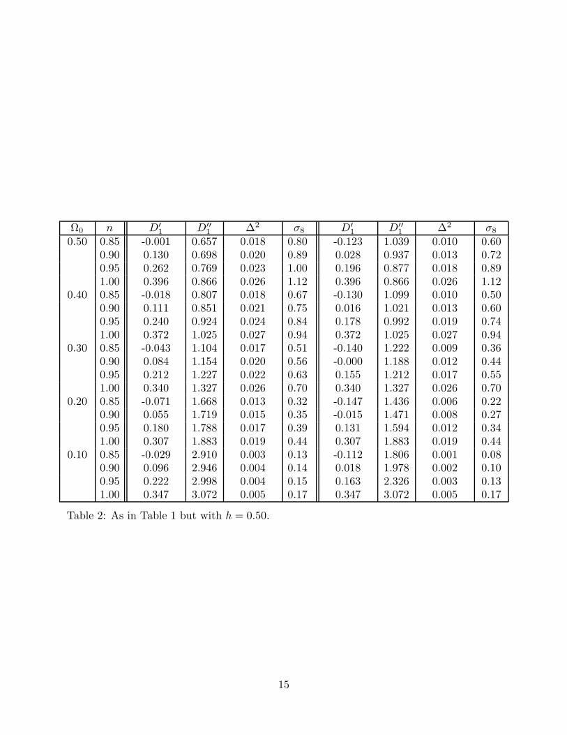
In Tables 1 and 2, and in Fig. 6,we show the normalization of the matter powerspectrum for a range of models where the CMB normalization (C10) is held fixed. Wequote both the value of the RMS density fluctuation at 0.028hMpc−1 (large-scale) and σ8

(small-scale). For comparison, Peacock & Dodds (1994) give

∆2(

k = 0.028hMpc−1)

≡dσ2

ρ

d ln k= (0.0087 ± 0.0023)Ω−0.3

0 . (18)

10

There are many determinations of σ8; we quote here those from Peacock & Dodds (1994)

σ8 = 0.75Ω−0.150 (19)

and cluster abundances (White, Efstathiou & Frenk 1993)

σ8 = 0.57Ω−0.560 (20)

where the scaling with Ω0 in both cases refers to models with Ω0+ΩΛ = 1. These values areconsistent with those inferred from large-scale flows (Dekel 1994) and direct observations(Loveday et al. 1992). In Fig. 7 we compare these observations with the COBE-normalizedvalues of σ8 for a range of ΛCDM models.

Conclusions

The COBE data forms a unique and valuable resource for the study of inhomogeneouscosmology. To fully exploit this hard won information we need to go beyond methods ofnormalizing theories of structure formation which use only gross properties of the data(such as the RMS fluctuation). In this paper we have presented a model independentmethod of parameterizing the COBE data, and discussed the normalization of the radiationand matter power spectra for a range of theoretically interesting models. In addition weconsidered the question of the goodness of fit of some commonly adopted models to thedata from two complementary statistical standpoints.

Acknowledgments

We thank Douglas Scott for useful conversations and Joe Silk for suggesting we includea tensor contribution to the Λ models. We would also like to thank Ned Wright forcomments on the manuscript and Section 3 in particular. The COBE data sets weredeveloped by the NASA Goddard Space Flight Center under the guidance of the COBEScience Working Group and were provided by the NSSDC. This work was supported inpart by grants from the NSF and DOE.

11

Appendix

In this appendix we make some comments about the fluctuation spectrum in an openuniverse. The material is taken from the work of Lyth & Stewart (1990), Ratra & Pee-bles (1994, and references therein), Bucher et al. (1995) and Lyth & Woszczyna (1995).These papers are sophisticated and rigorous treatments of the subject, and consequentlyare somewhat lengthy and technical in parts. Here we try to give a flavor of the problem,building on the rigorous results of those works. We will proceed in historical order.

We start by recalling a few points about inflationary cosmology. In an inflationarytheory with Ω0 = 1, quantum fluctuations during inflation give rise to density and poten-tial fluctuations today (see e.g. Olive 1990, Mukhanov et al. 1992, Kolb & Turner 1990,Linde 1990 and references therein). The amplitude of the fluctuations is set by the Hub-ble constant, Hinf , when the perturbation crosses out of the horizon, with larger scales(today) crossing the horizon earlier during inflation. If the potential of the inflaton (andhence Hinf) does not change very much during the time fluctuations on the relevant scalesare produced (exponential inflation) one obtains a scale-invariant spectrum of fluctuations:δ2 ∝ k. In terms of potential fluctuations, which are the perturbations which enter theunderlying metric and are in some sense more fundamental than the density perturbations,this corresponds to δΦ =constant ∝ Hinf/mPl. (This spectrum is therefore described asscale invariant.) In Lyth & Stewart (1990) it was shown that, for scales which entered thehorizon “early” when curvature could be neglected, δΦ =constant for Ω0 < 1 also. Thetransformation from this statement about the fluctuations in Φ per logarithmic intervalto one about P (k) proceeds in two steps. First, we relate the density perturbations tothe potential fluctuations through Poisson’s equation, which in an open universe reads(Mukhanov et al. 1992)

(

k2 − 3K)

δΦk = 4πa2ρδk (A1)

where the curvature scale is K = H20 (Ω0 − 1) as before. Second, we note that in an

open universe, the eigenfunctions of the operator ∇2 with eigenvalues k ≥√−K form

a complete set (Lifshitz & Khalatnikov 1963, Harrison 1970, Abbott & Schaefer 1986).Thus we can expand all perturbations in term of these eigenfunctions. It is convenient tointroduce the new variable q2 = k2/(−K)− 1 which runs from 0 to ∞. [In order to obtainthe most general gaussian random field in an open Universe, one must in general includethe eigenfunctions with 0 ≤ k ≤

√−K ; however, for fluctuations generated by inflation

only modes with k ≥√−K are excited (Lyth & Woszczyna 1995)]. Recall it is δΦ2

kdk/kor P (k)d3k which gives the physical fluctuations, so we need to compare the power perlogarithmic interval in k to the volume element in the two coordinates

4πdk

k=

d3k

k3=

d3q

q(q2 + 1). (A2)

Writing k2 − 3K ∝ q2 + 4, and using the Poisson equation to translate from potentialfluctuations (squared, per ln k) to density fluctuations (squared, per d3q) we have

P (q) ∝ (q2 + 4)2

q(q2 + 1)(A3)

12

which is the result of Lyth & Stewart (1990). Ratra & Peebles (1994) performed a calcu-lation of fluctuations from a linear potential in which they showed that this result extendsto all q, not just those which entered the horizon while Ω ≃ 1.

In a recent paper, Bucher et al. (1995) consider an explicit model for open universeinflation. [A similar calculation has been done by Yamamoto et al. (1995)]. In this modelthe inflaton first gets trapped in a false minimum of the potential for some time. Duringthis time the universe inflates exponentially. The quantum fluctuations in the zero pointenergy are (power-law) suppressed by the existence of a mass gap (the inflaton has amass, since the potential has curvature at the minimum V (ϕ) = V0 + m2ϕ2/2 + · · ·). Theinflaton then tunnels through the barrier in the standard semi-classical way (c.f. nucleardecay) and nucleates a bubble of Ω0 ≃ 0 universe. As the potential rolls slowly from itspost-tunneling value to the minimum of the potential more fluctuations are generated.The upshot of this, after a strenuous calculation, is that the potential fluctuations onsmall scales are δΦ =constant, as before. On larger scales, corresponding to earlier timesduring inflation, the potential fluctuations are either enhanced or reduced, depending onthe value of m in the potential. For the value of m considered in Bucher et al. (1995) onefinds an enhancement by an extra factor of q−1 on very large scales. It is worthwhile tostress however that the Cℓ are relatively insensitive to q ∼< 1 within reasonable variationsin P (q).

The issue of fluctuations in open-universe inflation is not settled. Further theoreticalwork is required to determine whether inflation makes a unique prediction for the fluctua-tion spectrum in an open Universe, or whether we must rely on experiments to distinguishamong the different possibilities. Should the power spectra rise as q−1 or q−2 on largescales, as currently predicted, then models with Ω0 between 0.1 and 0.3 will be disfavoredby the COBE data.

13

Tables

Ω0 n D′

1 D′′

1 ∆2 σ8 D′

1 D′′

1 ∆2 σ8

0.50 0.85 -0.079 0.476 0.027 1.45 -0.186 0.910 0.015 1.080.90 0.046 0.503 0.031 1.62 -0.043 0.785 0.020 1.310.95 0.172 0.557 0.036 1.82 0.115 0.693 0.028 1.621.00 0.298 0.635 0.040 2.05 0.298 0.635 0.040 2.05

0.40 0.85 -0.110 0.600 0.030 1.29 -0.202 0.955 0.016 0.950.90 0.012 0.631 0.034 1.45 -0.065 0.853 0.022 1.150.95 0.135 0.685 0.039 1.62 0.084 0.787 0.030 1.431.00 0.258 0.767 0.045 1.82 0.258 0.767 0.045 1.82

0.30 0.85 -0.159 0.853 0.032 1.10 -0.225 1.058 0.016 0.790.90 -0.040 0.885 0.036 1.24 -0.097 0.991 0.022 0.970.95 0.080 0.944 0.041 1.39 0.041 0.975 0.031 1.211.00 0.201 1.022 0.047 1.56 0.201 1.022 0.047 1.56

0.20 0.85 -0.240 1.338 0.029 0.82 -0.258 1.237 0.014 0.560.90 -0.124 1.366 0.033 0.92 -0.143 1.229 0.019 0.690.95 -0.008 1.415 0.038 1.03 -0.023 1.295 0.027 0.881.00 0.108 1.485 0.043 1.15 0.108 1.485 0.043 1.15

0.10 0.85 -0.342 2.455 0.014 0.33 -0.275 1.561 0.006 0.210.90 -0.227 2.462 0.016 0.37 -0.176 1.673 0.008 0.260.95 -0.113 2.485 0.019 0.41 -0.082 1.931 0.012 0.331.00 0.000 2.527 0.022 0.46 0.000 2.527 0.022 0.46

Table 1: The shape of the radiation power spectrum in a ΛCDM model with h = 0.75.Also shown is the matter power spectrum normalization with the radiation normalized toC10 = 10−11. For the tilted models we show the results with (right columns) and without(left columns) a gravity wave component with CT

2 /CS2 = 7(1 − n).

14

Ω0 n D′

1 D′′

1 ∆2 σ8 D′

1 D′′

1 ∆2 σ8

0.50 0.85 -0.001 0.657 0.018 0.80 -0.123 1.039 0.010 0.600.90 0.130 0.698 0.020 0.89 0.028 0.937 0.013 0.720.95 0.262 0.769 0.023 1.00 0.196 0.877 0.018 0.891.00 0.396 0.866 0.026 1.12 0.396 0.866 0.026 1.12

0.40 0.85 -0.018 0.807 0.018 0.67 -0.130 1.099 0.010 0.500.90 0.111 0.851 0.021 0.75 0.016 1.021 0.013 0.600.95 0.240 0.924 0.024 0.84 0.178 0.992 0.019 0.741.00 0.372 1.025 0.027 0.94 0.372 1.025 0.027 0.94

0.30 0.85 -0.043 1.104 0.017 0.51 -0.140 1.222 0.009 0.360.90 0.084 1.154 0.020 0.56 -0.000 1.188 0.012 0.440.95 0.212 1.227 0.022 0.63 0.155 1.212 0.017 0.551.00 0.340 1.327 0.026 0.70 0.340 1.327 0.026 0.70

0.20 0.85 -0.071 1.668 0.013 0.32 -0.147 1.436 0.006 0.220.90 0.055 1.719 0.015 0.35 -0.015 1.471 0.008 0.270.95 0.180 1.788 0.017 0.39 0.131 1.594 0.012 0.341.00 0.307 1.883 0.019 0.44 0.307 1.883 0.019 0.44

0.10 0.85 -0.029 2.910 0.003 0.13 -0.112 1.806 0.001 0.080.90 0.096 2.946 0.004 0.14 0.018 1.978 0.002 0.100.95 0.222 2.998 0.004 0.15 0.163 2.326 0.003 0.131.00 0.347 3.072 0.005 0.17 0.347 3.072 0.005 0.17

Table 2: As in Table 1 but with h = 0.50.

15

Model D′

1 D′′

1 L ConsistencyProbability

1 0.4 -1.6 3.29 78.0%2 0 0 1.00 86.3%3 -0.5 3.5 0.091 93.0%4 -2 0 0.014 97.2%5 -0.342 2.455 0.186 92.4%6 -0.275 1.561 0.310 91.4%

Table 3: Bayesian and frequentist measures of goodness of fit for six cosmological models(see text). The shape parameters D′

1 and D′′

1 are defined in the text. L denotes theBayesian peak likelihood, normalized so that a pure Harrison-Zel’dovich Sachs-Wolfe modelhas L = 1. The consistency probability is the percentage of simulated data sets for whichthe goodness-of-fit parameter η defined in Eq. 14 is less than the value found for the realdata.

16

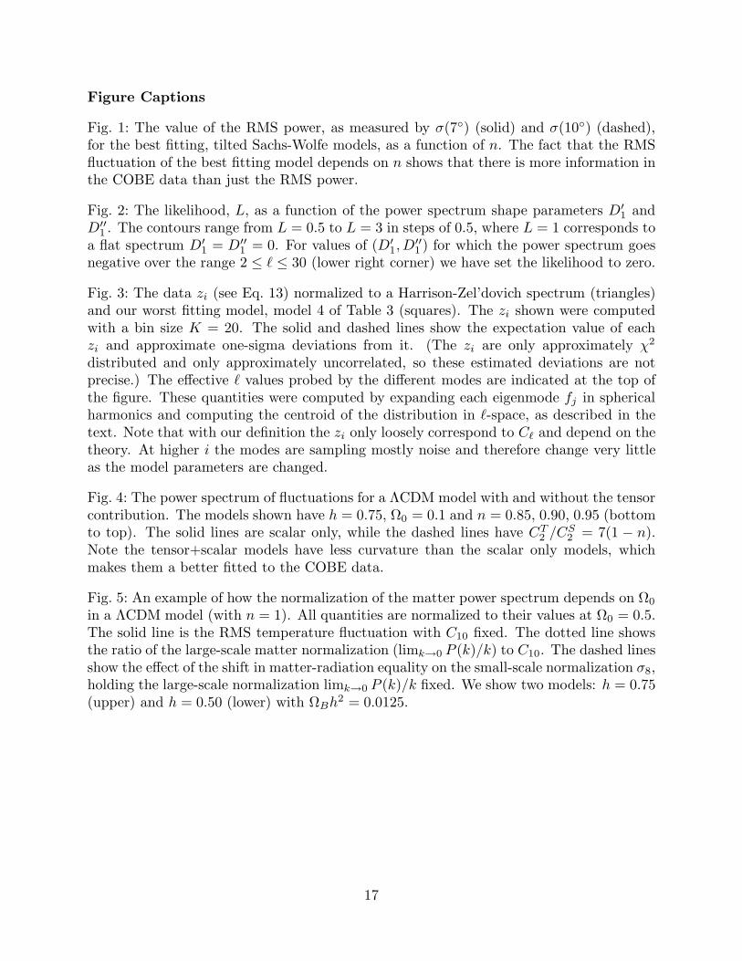
Figure Captions

Fig. 1: The value of the RMS power, as measured by σ(7) (solid) and σ(10) (dashed),for the best fitting, tilted Sachs-Wolfe models, as a function of n. The fact that the RMSfluctuation of the best fitting model depends on n shows that there is more information inthe COBE data than just the RMS power.

Fig. 2: The likelihood, L, as a function of the power spectrum shape parameters D′

1 andD′′

1 . The contours range from L = 0.5 to L = 3 in steps of 0.5, where L = 1 corresponds toa flat spectrum D′

1 = D′′

1 = 0. For values of (D′

1, D′′

1 ) for which the power spectrum goesnegative over the range 2 ≤ ℓ ≤ 30 (lower right corner) we have set the likelihood to zero.

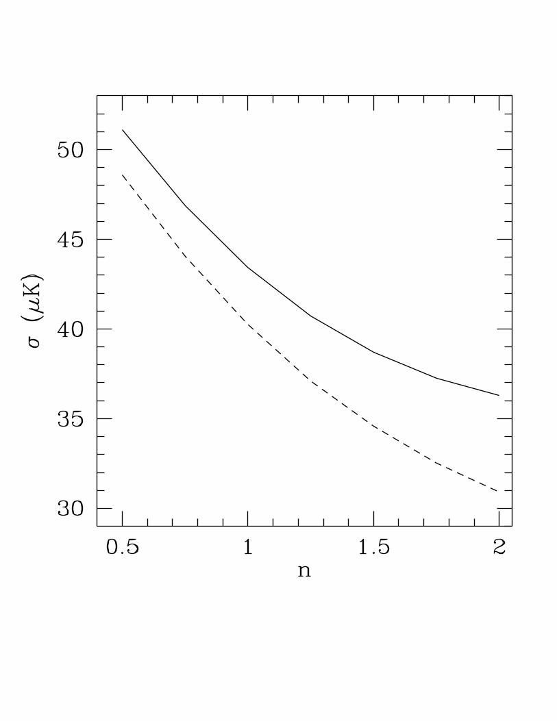
Fig. 3: The data zi (see Eq. 13) normalized to a Harrison-Zel’dovich spectrum (triangles)and our worst fitting model, model 4 of Table 3 (squares). The zi shown were computedwith a bin size K = 20. The solid and dashed lines show the expectation value of eachzi and approximate one-sigma deviations from it. (The zi are only approximately χ2

distributed and only approximately uncorrelated, so these estimated deviations are notprecise.) The effective ℓ values probed by the different modes are indicated at the top ofthe figure. These quantities were computed by expanding each eigenmode fj in sphericalharmonics and computing the centroid of the distribution in ℓ-space, as described in thetext. Note that with our definition the zi only loosely correspond to Cℓ and depend on thetheory. At higher i the modes are sampling mostly noise and therefore change very littleas the model parameters are changed.

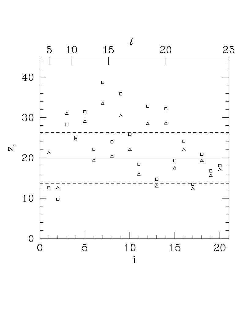
Fig. 4: The power spectrum of fluctuations for a ΛCDM model with and without the tensorcontribution. The models shown have h = 0.75, Ω0 = 0.1 and n = 0.85, 0.90, 0.95 (bottomto top). The solid lines are scalar only, while the dashed lines have CT

2 /CS2 = 7(1 − n).

Note the tensor+scalar models have less curvature than the scalar only models, whichmakes them a better fitted to the COBE data.

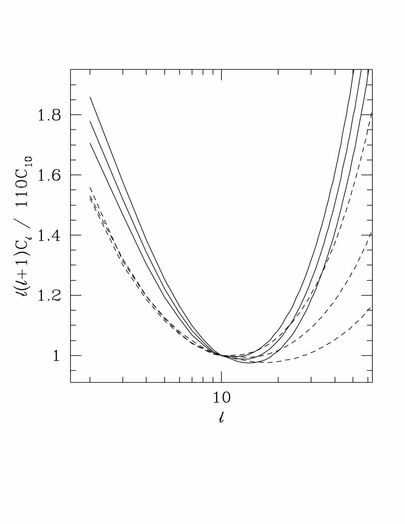
Fig. 5: An example of how the normalization of the matter power spectrum depends on Ω0

in a ΛCDM model (with n = 1). All quantities are normalized to their values at Ω0 = 0.5.The solid line is the RMS temperature fluctuation with C10 fixed. The dotted line showsthe ratio of the large-scale matter normalization (limk→0 P (k)/k) to C10. The dashed linesshow the effect of the shift in matter-radiation equality on the small-scale normalization σ8,holding the large-scale normalization limk→0 P (k)/k fixed. We show two models: h = 0.75(upper) and h = 0.50 (lower) with ΩBh2 = 0.0125.

17

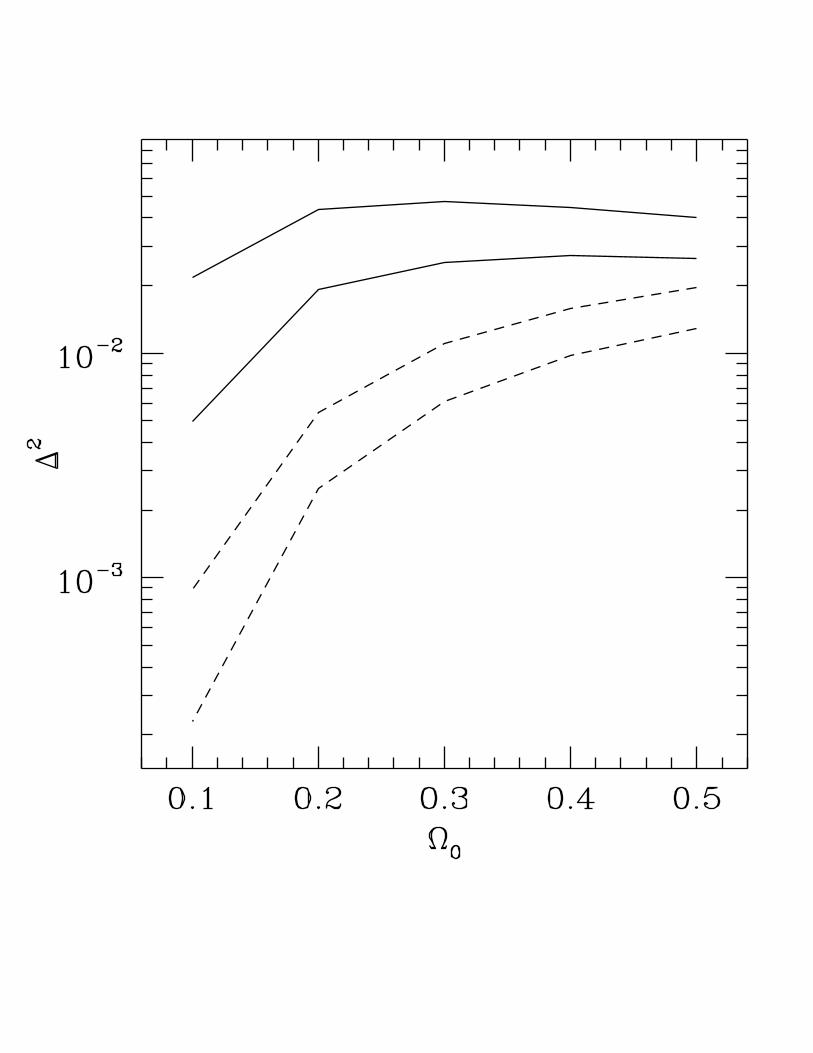
Fig. 6: The normalization, ∆2(0.028hMpc−1), as a function of Ω0 for open CDM (dashed)and ΛCDM (solid) models normalized to C10 = 10−11. In both cases the upper curves arefor h = 0.75 and the lower curves are for h = 0.50, both with ΩBh2 = 0.0125.

Fig. 7: The small scale normalization σ8 vs Ω0 in ΛCDM models, with normalization setby Eq. 9. The dashed lines assume all the contribution to the temperature fluctuationsmeasured by COBE come from scalar perturbations; the dotted lines are scalars + tensorswith CT

2 /CS2 = 7(1− n). Slope (n) increases from 0.85 to 1.00 in steps of 0.05 with lowest

n being lowest σ8. The two solid lines are two observational determinations of σ8, the topline from cluster abundances and the bottom line from large scale structure (i.e. Eqs. 19,20).

18

References

Abbott, L. F., & Schaefer, R. K., 1986, ApJ, 308, 546

Banday, A.J. et al. 1994, ApJ, 436, L99

Bennett, C. L., et al. 1994, ApJ, 436, 423

Bucher, M., Goldhaber, A., & Turok, N., 1995, Phys. Rev., in press

Bunn, E., Scott, D., & White, M., 1995, ApJ, 441, L9

Bunn, E., & Sugiyama, N., 1995, ApJ, 446, 49

Carroll, S. M., Press, W. H., & Turner, E. L., 1992, Ann. Rev. A. & Astrophys, 30, 499

Crittenden, R., Bond, J. R., Davis, R. L., Efstathiou, G., & Steinhardt, P. J., 1993, Phys.

Rev. Lett., 71, 324

Davis, R. L., Hodges, H. M., Smoot, G. F., Steinhardt, P. J., Turner, M. S., 1992, Phys.

Rev. Lett., 69, 1856 (erratum: 70:1733)

Efstathiou, G., Bond, J. R., & White, S. D. M., 1992, MNRAS, 258, 1 p

Gorski, K. M., et al. 1994, ApJ, 430, L89

Gorski, K. M., et al. 1995a, COBE, preprint

Gorski, K. M., et al. 1995b, in, preparation

Hu, W. & Sugiyama, N. 1995, ApJ, 444, 489

Karhunen, K. 1947, Uber lineare Methoden in der Wahrschleinlichkeitsrechnung, Helsinki:Kirjapaino oy. sana

Kofman, L., Gnedin, N. Y., & Bahcall, N. A., 1993, ApJ, 413, 1

Kofman, L., & Starobinsky, A., 1985, Sov. Astron. Lett., 11, 271

Kolb, E. W., & Vadas, S., 1993, Phys. Rev., D50, 2479

Kolb, E. W., & Turner, M. S., 1990, The Early Universe, Addison Wesley

Harrison, E. R., 1970, Phys. Rev., D1, 2726

Liddle, A. R., & Lyth, D. H., 1992, Phys. Lett., B291, 391

Liddle, A. R., & Lyth, D. H., 1995, MNRAS, in press

Lifshitz, E. M., & Khalatnikov, I. M., 1963, Adv. Phys., 12, 185

Linde, A., 1990, Particle Physics and Inflationary Cosmology, Harwood Academic

Lineweaver, C.H., Smoot, G.F., Bennett, C.L., Wright, E.L., Tenorio, L., Kogut, A.,Keegstra, P.B., Hinshaw, G., & Banday, A.J., 1994, ApJ, 436, 452

Loveday, J. S., Efstathiou, G., Peterson, B. A. & Maddox, S. J., 1992, ApJ, 400, L43

Lyth, D. H. & Stewart, E., 1990, Phys. Lett., B252, 336

Lyth, D. H. & Woszczyna, A., 1995, Lancaster, preprint

Mukhanov, V. F., Feldman, H. A., & Brandenberger, R. H., 1992, Phys. Rep., 215, 203

Olive, K., 1990, Phys. Rep., 190, 307

Peacock, J. A. & Dodds, S. J., 1994, MNRAS, 267, 1020

19

Peebles, P. J. E., 1993, Principles of Physical Cosmology, Princeton UP

Ratra, B., & Peebles, P. J. E., 1994, ApJ, 432, L5

Sachs, R. K., & Wolfe, A. M., 1967, Ap. J., 147, 73

Smoot, G., et al., 1992, ApJ, 396, L1

Tegmark, M. & Bunn, E.F., 1995, Berkeley, preprint

Thierren, C.W., 1992, Discrete Random Signals and Statistical Signal Processing, Prentice-Hall

Turner, M. S., White, M., & Lidsey, J. E., 1993, Phys. Rev., D48, 4613

White, M., 1994, Astron. & Astrophys., 290, L1

White, M., Scott, D., & Silk, J., 1994, Ann. Rev. A. & Astrophys., 32, 319

White, S.D.M., Efstathiou, G., & Frenk C. 1993, MNRAS, 262, 1023

Wright, E. L., Smoot, G. F., Bennett, C. L., & Lubin, P. M., 1994, ApJ, 436, 443

Yamamoto, K., Sasaki, M., & Tanaka, T., 1995, Kyoto, preprint

20

arX

iv:a

stro

-ph/

9503

054v

3 1

1 N

ov 1

995

Erratum

The COBE Normalization of CMB AnisotropiesMartin White & Emory Bunn

Ap. J. 450, 477 (1995)

In tables 1 & 2 the quoted values of ∆2 and σ8 assume a tensor-to-scalar ratioCT

2 /CS2 = 7(1 − n). This is the correct lowest order (in an expansion in 1 − n) ex-

pression for the tensor-to-scalar ratio for Ω0 = 1. However the projection from the k-spaceinflationary prediction onto the quadrupole, i.e. ℓ = 2 mode, has a dependence on ΩΛ andn, which was neglected in calculating the entries in the tables. The “correction factor”,fT/S(ΩΛ, n), defined through

CT2 /CS

2 = 7 (1 − n) fT/S(ΩΛ, n)

can be well fit by

fT/S(ΩΛ, n) = 0.97 − 0.58(1− n) + 0.25ΩΛ −[

1 − 1.1(1 − n) + 0.28(1− n)2]

Ω2Λ .

This expression includes both the full n dependence (i.e. beyond leading order in 1−n) ofpower-law inflation, for which exact expressions are available, and the ISW contributionto CS

2 . To good approximation the values of ∆2 quoted in the tables should be multipliedby

1 + 7(1 − n)

1 + 7(1 − n)fT/S

and the values of σ8 by the square root of this. For reasonable values of ΩΛ and n thisamounts to a <∼ 10% correction.

1