the centre matters for the periphery of europe: the

August 2014

The Centre Matters for the Periphery of Europe: The Predictive Ability of

a GZ-Type Spread for Economic Activity in Europe

by

Alfred V Guender Bernard Tolan*

University of Canterbury New Zealand Treasury

Christchurch, New Zealand Wellington, New Zealand

& Freie Universität Berlin, Germany

JEL Codes: E3, E4, G1

Key Words: corporate bond yield spread, predictive content, economic activity in Europe,

Financial and Debt Crisis.

The views expressed in this paper are those of the authors alone and do not reflect the views of NZ Treasury.

The authors wish to thank Richard Froyen, Alexander Jung, Philip Meguire and the seminar participants at

Victoria University, the University of Antwerp, and the Free University of Berlin for helpful comments.

2

The recent twin financial crises have turned the spotlight on asset prices and the sources of

corporate borrowing in Europe. Since 2007 the financial press has observed and regularly

commented upon two trends that are slowly changing the traditional financial landscape of

Europe. First, private-sector companies are increasingly turning towards the bond market to

raise financial capital, especially during times of financial strain. The move towards bond

financing may only be temporary though since traditionally European firms have relied

predominantly on bank loans as a source of finance.1 Only a few years ago, in the first quarter

of 2007, the volume of bank loans exceeded bond issuance fivefold. Two years later, in the

midst of the Global Financial Crisis, bonds began to dominate bank loans as a source of

corporate funding. But bank loans did recover their premier status as the effects of the crisis

receded. In the first quarter of 2012 European firms again tapped more into the bond market

than commercial banks, borrowing US$179.5 billion on the bond market compared to $112.9

billion from banks.2 Second, the financial landscape of Europe is becoming again more

fragmented, a sign that the process of financial integration has been disrupted. In the wake of

the Global Financial Crisis and the Sovereign Debt Crisis, borrowing costs in the countries on

the European periphery have increased dramatically relative to the cost of borrowing in the

centre of Europe. Firms in southern European countries and Ireland have faced higher interest

rates than firms in Germany because risk premia in the weaker economies on the periphery

have surged relative to the centre and because credit conditions have been tighter in the

former compared to the latter. In November 2010, companies in Spain, Portugal and Ireland

were virtually shut out of the corporate bond market when fear of sovereign default spilled

from the sovereign debt market to the corporate debt market.3 Bank credit, too, has been

squeezed in the periphery countries as banks in central and northern Europe have taken steps

to cut back their cross-border exposure.4 As a direct consequence of the Sovereign Debt

Crisis, corporate borrowing rates on bank loans in Spain and Italy have risen much faster than

in Germany. Indeed in the third quarter of 2012 they stood at 6.5 % and 6.24 %, respectively,

their highest level in both countries since late 2008 while in Germany the rate was just 4.04

% and thus only slightly above its minimum since late 2008.5

1 Wall Street Journal, “Bonds with Banks Fraying,” April 10, 2012.

2 Ibid.

3 Financial Times, “European Company Borrowing Costs Rise,” November 30, 2010. The article reports that

“the last bond issue from a company domiciled in Spain, Portugal or Ireland came from Iberdrola, the Spanish

utility, on October 6th

.” Thus no corporate bond placement was effected in almost two months. 4 Financial Times, “Loan Rates Point to Eurozone Fractures,” September 3, 2012. The rates quoted are the

average rate on loans to non-financial corporations, 1-5 years, up to € 1 million in value. 5 Ibid.

3

This paper examines whether information from bond markets provides a reliable signal for

future economic activity in Europe. It evaluates the marginal predictive content and economic

significance of a risk-adjusted credit spread in five European countries from the early 1990s

to the recent past. Following the lead of the financial press, we distinguish between the

periphery and the centre of Europe. Four countries - Ireland, Italy, Portugal, and Spain - are

members of the European periphery while Germany represents the centre of Europe.6 The

credit spread is defined as the average of yields on outstanding corporate bonds in a country

on the European periphery less a riskless yield. The riskless yield is computed using data

from the zero-coupon curve of German government bonds (Bunds). German Bunds are thus

deemed to be safe havens. The intuition behind the credit spread is straightforward. In times

of financial stress, credit conditions tighten. The supply of credit decreases because the

creditworthiness of firms deteriorates. The risk premium on privately issued bonds rises,

leading to a widening in the spread between risky private bond yields and the riskless yield.7

Worsening credit conditions in turn reduce spending and consequently real economic activity

declines.8

The inclusion of the bond yield spread (henceforth called GZ-spread because it follows the

“bottom-up” approach proposed by Gilchrist and Zakrašjek (2012)) improves markedly the

goodness of fit of the forecasting equation for economic activity in countries on the European

periphery.9 The within-sample forecasting ability of the GZ-spread is remarkable, both over

the whole sample period and a sub-sample period marking the effective beginning of the

Economic and Monetary Union of Europe (EMU) in 1999. Indeed since the establishment of

the EMU its economic significance in predicting future economic activity has increased in

6 Ideally, we would have included Greece in our examination. Unfortunately, data constraints made this

impossible. Germany is chosen to be the centre on account of it having the largest economy in Europe and its

triple A credit rating. 7 This is the gist of the Financial Accelerator effect (Bernanke and Gilchrist (1996), Bernanke, Gertler, and

Gilchrist (1999)). For a non-technical analysis, see Bernanke and Gertler (1995). 8 The healthiness of financial intermediaries may deteriorate as well. Shrinking balance sheets reduce the size of

loan portfolios, driving up other credit spreads such as the LIBOR-OIS spread. 9 There has been a long-standing interest in the predictive ability of various financial indicators for economic

activity and inflation. Among the most frequently used proxies for monetary conditions are the yield spread on

long-term and short-term government bonds (Bernanke (1988), Harvey (1988), Estrella and Hardouvelis (1991),

and others) and the risk spread, defined as the difference between the yield on short-term commercial paper and

the yield on Treasury Bills of the same maturity (Friedman and Kuttner (1992), (1998), Emery (1996)). Moersch

(1996) finds that money market spreads predict output better than other spreads along the yield curve. Various

US bond yield spreads (long-term, high yield) figure prominently in Gertler and Lown (1999), Mody and Taylor

(2004) and King et al (2007). De Bondt (2004) analyses bond yield spreads in Europe. More recent

contributions such as Mueller (2009) also examine corporate bond yield spreads defined along rating categories

in the context of a macro-finance term structure model of the type proposed by Ang, Piazzesi, and Wei (2006).

A comprehensive survey of the literature on the role of asset prices in forecasting economic activity is by Stock

and Watson (2003).

4

most countries on the European periphery that have been hit hard by the recent turmoil in

financial markets. The marginal predictive content of the GZ-spread for changes in economic

activity in these countries is impressive even after accounting for the effect of standard

monetary policy measures such as the slope of the term spread and a short-term money

market rate.

Like Gilchrist and Zakrašjek (2012), we also examine the predictive content of a country-

specific GZ-spread. The GZ-spread constructed for Germany consists of the difference

between the yields on German corporate bonds and the riskless German Bund yield.10

The

predictive ability of the “internal” GZ-spread for economic activity in Germany is spotty. The

GZ-spread matters for the growth rate of industrial production and real GDP over some

horizons but appears to have no bearing on future changes in the rate of unemployment.

In the next section, we explain in greater detail the calculation of the GZ-type spread that is

used in the forecasting equation. Section III presents summary statistics of the data and the

GZ-spread. The specification of the forecasting equation is explained in detail in Section IV.

The predictive content of the GZ-spread and standard measures of monetary policy for

economic activity is examined in Section V. Section VI offers a brief conclusion.

II. Calculation of the GZ-Spread

Except for the German GZ-spread, our method of constructing the GZ-spread is somewhat

different from the one proposed by Gilchrist and Zakrašjek (2012). Our method uses rates

from the German zero curve as reference rates to calculate the price of a riskless bond in a

country on the European periphery. This synthetic bond has the same coupon schedule as a

given corporate bond issued in a country on the European periphery. Unlike Gilchrist and

Zakrašjek, we exclude bonds with embedded options.

The procedure we follow to calculate the GZ-spread comprises two parts. First, we calculate

the monthly spread between the yield on corporate bond j in country a and the risk-free

German yield at time t. Second, we calculate the GZ-spread at the country level by averaging

the individual bond spreads in country a in a given month. This procedure is set out in detail

below.

10

Bleaney, Mizen, and Veleanu (2012) compose country-specific GZ-spreads in the spirit of Gilchrist and

Zakrašjek (2012) for a number of European countries. Their analysis of the predictive content of credit spreads

differs from ours in three important respects. They are: construction of the GZ-spread, countries included in the

study, and estimation method. According to the findings of their panel data study, the GZ-spread is a reliable

predictor of future economic activity in Europe.

5

We first obtain monthly yield-to-redemption data on senior, unsecured corporate bonds from

DataStream for every country in our sample (Portugal, Ireland, Italy, Spain and

Germany).Our sample period begins in 1990 shortly after German reunification, and spans

the transition to the Economic and Monetary Union and the Global Financial Crisis before

finishing in 2012 in the midst of the Sovereign Debt Crisis. Like Gilchrist and Zakrašjek, we

include bonds of only non-financial firms.

Next, we obtain the risk-free rate which we use to create the GZ spread at the ‘bond level’.

In order to obtain a risk-free rate without ‘duration bias,’ we require a German risk-free bond

with the same coupon schedule as corporate bond j in month t. Of course no such bond exists,

so we follow Gilchrist and Zakrašjek and create a ‘synthetic risk-free bond’. This synthetic

bond, in effect, is a German federal government bond with the same coupon schedule at time

t as corporate bond j.

To find the yield for the synthetic German security which matches corporate bond j in month

t, we first need to calculate its price. The price of corporate bond j in a given country at time

t,

, is calculated by applying the discount function, D(t) to a stream of s regular coupon

payments where C(s): s =1, 2…S , ( ) and ‘r’ is the yield to maturity:

∑ ( ) ( )

The price

of a synthetic German security at time t can be found by discounting

C(s) using s zero coupon risk-free interest rates. That is, ( ) where is the

German zero rate at time t with a maturity m corresponding to the time until coupon payment

s. For example, to find the price of the synthetic risk-free bond that corresponds to a

corporate bond that pays one coupon six months from today (time t) and matures in twelve

months, one performs the following calculation (assume coupon rate is 5% and last coupon is

paid at maturity with principal $1000):

where

today’s interest rate on a German zero coupon bond with a maturity of six months

(0.5 of a year).

6

today’s interest rate on a German zero coupon bond with a maturity of twelve

months.

the price of a synthetic risk-free security.

Note coupons are paid semi-annually in the example.

We obtain from a German zero curve downloaded from the Bundesbank website. For

each month, the zero curve plots German zero securities of ascending maturity (six months

up to thirty years in yearly intervals from one year up) on the x-axis and their corresponding

yields on the y-axis. Where necessary, we linearly interpolate to get the risk-free discount rate

with the exact same maturity as a given coupon payment.

Once we have the price of the German synthetic bond, we numerically solve for the yield-to-

maturity (this is just the internal rate of return). The result,

is the risk-free portion

of the ‘bond-level’ spread for bond j at time t.

Next, we calculate the risk-free rate for every bond in our sample using the method described

above.

We then subtract the risk-free rate from the yield on corporate bond j at time t in country a.

The result, , is the spread at the ‘bond level’:

The final step is to average the spread in country a at time t to create the GZ-spread at

the country level:

∑

the number of bond observations in month t.11

11

Since this spread is calculated in a cross-country context, the measured spread consists of a combination of

two components. One measures corporate credit risk while the other reflects peripheral country risk.

7

For example, to find the Italian GZ spread in January 2007, average all of available

observations of the Italian bond level spreads in that month. Thus the credit spread is

representative of the entire maturity and credit quality spectrum as emphasized by Gilchrist

and Zakrašjek (2012). We also follow their example of eliminating from the sample bonds

with remaining terms of maturity of less than one year or more than 30 years. In the same

vein, extreme observations of the GZ-spread, i.e. those below 0.05 percent or above 35

percent were scrapped from the sample.

III. The GZ-Spread in the Centre and on the Periphery of Europe: Basic Facts

Table 1A provides summary statistics of the data used in the empirical analysis. The number

of bond-issuing firms varies from a low of 13 for Ireland and Portugal to a high of 62 for

Germany. The number of corporate bonds issued during the sample period, which is country-

specific, ranges from a low of 42 for Portugal to a high 330 for Germany. The mean yield is

highest in Ireland and lowest in Germany.12

The mean maturity at issue of bonds is far longer

in Spain (11.81 yrs.) and Ireland (12.76 yrs.) than in Germany where it is slightly below

seven years.13

Summary statistics of the GZ-spread for Germany, Ireland, Italy, Portugal, and

Spain appear in Table 1B. Data limitations for Spain and Portugal restrict a cross-country

comparison of the summary statistics over the 1990-2012 sample period to Italy, Ireland, and

Germany. The GZ-spread can be calculated for Spain only from 1996 onward; for Portugal

the GZ-spread starts even later, in April 1999.

Inspection of Table 1B.1 reveals that the GZ-spread is considerably lower and less variable in

Germany compared to Italy and Ireland over the whole sample period. Comparing Tables

1B.2 and 1B.3, we observe that the period since the start of the Economic and Monetary

Union in 1999 has seen a lower and more stable GZ-spread in Italy and Ireland.14

Since 1999,

the volatility of the GZ-spread has been reduced by half in Germany while its mean has risen

slightly compared to the pre-1999 period. Breaking down the EMU Period into a pre-Crisis

(1999:01-2007:07) period and a Crisis period (2007:08-2012:08) shows that during the Crisis

12

It may seem strange that corporate bonds issued by Irish firms enjoy the highest credit rating. It must be borne

in mind, however, that credit ratings are not available for all firms at all times. 13

The maturity profile of corporate bonds included in the sample corresponds broadly to that reported by the

European Central Bank in its February 2012 Bulletin. Over the 1999-2007 period the average maturity of

corporate bonds was shortest in Germany at 4.7 years and highest in Ireland at 8.8 years. 14

Strictly speaking, January 1, 1999 marks the beginning of the third stage of the Economic and Monetary

Union. On this date the Euro officially replaced the Ecu as the official currency of the union. For the first three

years the Euro served only as a unit of account. Euro coins and banknotes were not introduced until January 1,

2002.

8

period the mean of the GZ-spread rises in all five countries. The rise is most pronounced in

Portugal where the GZ-spread surges upward by almost 300 basis points, followed by

Ireland, Spain, and Italy while in Germany the GZ-spread ratchets upward by only 80 basis

points. Large increases in the variability of the GZ-spread are observed in Portugal and Spain.

Even in Germany the standard deviation of the GZ-spread nearly doubles during the Crisis

period. Notice though that the GZ-spread peaks during the Crisis period only in Portugal,

Spain, and Ireland when all observations over the whole sample period are taken into

account. Evidently, during the Crisis period credit conditions worsen by more in the smaller

and medium-size economies on the periphery relative to the larger ones.

The GZ-Spread during Recessions

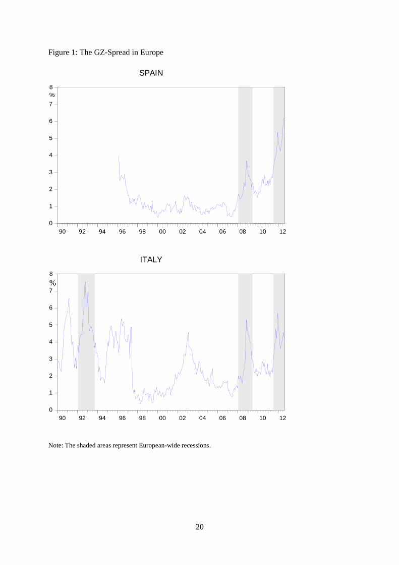
Figures 1 - 5 track the behaviour of the GZ-spread in the five countries over the respective

sample period. The individual graphs show clearly that the GZ-spread is at quite elevated

levels in Ireland and Italy at the beginning of the 1990s and in Germany from 1992 to the first

quarter of 1996.15

The spread is also relatively high initially in Spain before it drops off

markedly in 1997. The GZ-spread never rises above 200 basis points and is relatively stable

in Portugal before the Crisis period. Most importantly, however, the five graphs show the

countercyclical behaviour of the GZ-spread: it tends to rise before recessions begin and

surges dramatically during recessions when perceived risk increases. The recessions appear

as shaded areas in each figure. The CEPR Business Cycle Committee has identified three

European-wide recessions over the 1991-2012 sample period. The beginning and end of each

recession are:16

1992 Q1 – 1993 Q3 2008 Q1 – 2009 Q2 2011 Q3 – end of sample period.

The Crisis period includes two recessions. As a result there are twin peaks in the GZ-spread

during the Crisis period. Notice, however, that there is no clear-cut, systematic evidence

across the five countries that the GZ-spread widens more during the Sovereign Debt Crisis

than the Global Financial Crisis (or vice versa). It is true that the former crisis causes far

greater surges in the GZ-Spread than the latter in Portugal and Spain and a slightly larger

spike in Italy but the pattern is just the reverse for Germany and Ireland where larger

15

For Germany one also observes a steep increase in the GZ-spread in 1998 around the time of the Russian

Default. 16

The first recession preceded Black Wednesday in September 1992 when the European Exchange Rate

Mechanism came under attack. The second recession was triggered off by the Global Financial Crisis while the

third came upon the heels of the European Sovereign Debt Crisis.

9

increases in the GZ-spread are manifest during the Global Financial Crisis compared to the

Sovereign Debt Crisis.

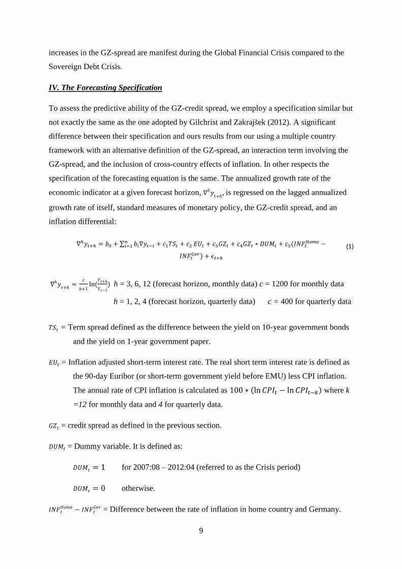
IV. The Forecasting Specification

To assess the predictive ability of the GZ-credit spread, we employ a specification similar but

not exactly the same as the one adopted by Gilchrist and Zakrajšek (2012). A significant

difference between their specification and ours results from our using a multiple country

framework with an alternative definition of the GZ-spread, an interaction term involving the

GZ-spread, and the inclusion of cross-country effects of inflation. In other respects the

specification of the forecasting equation is the same. The annualized growth rate of the

economic indicator at a given forecast horizon, is regressed on the lagged annualized

growth rate of itself, standard measures of monetary policy, the GZ-credit spread, and an

inflation differential:

∑

(

)

(1)

(

) h = 3, 6, 12 (forecast horizon, monthly data) c = 1200 for monthly data

h = 1, 2, 4 (forecast horizon, quarterly data) c = 400 for quarterly data

= Term spread defined as the difference between the yield on 10-year government bonds

and the yield on 1-year government paper.

= Inflation adjusted short-term interest rate. The real short term interest rate is defined as

the 90-day Euribor (or short-term government yield before EMU) less CPI inflation.

The annual rate of CPI inflation is calculated as ( ) where k

=12 for monthly data and 4 for quarterly data.

= credit spread as defined in the previous section.

= Dummy variable. It is defined as:

for 2007:08 – 2012:04 (referred to as the Crisis period)

otherwise.

= Difference between the rate of inflation in home country and Germany.

10

According to conventional wisdom, a tightening of monetary policy leads to a flattening of

the yield curve, a decrease in the term spread, and a subsequent decrease in economic

activity. Increases in the short-term real interest rate and future economic activity are

inversely related. Increases in the GZ-spread reflect a tightening of credit conditions in

financial markets and foreshadow a downturn in economic activity. We are agnostic about the

effects of higher relative inflation on future economic activity. On the one hand, higher

inflation in the home country relative to Germany is expected to harm the growth prospects

of the home country as higher relative inflation imparts a competitive cost disadvantage and

increases transaction costs. On the other hand, higher relative inflation in the home country

may be a signal that the home country is in an expansionary phase of the business cycle.

V. The Predictive Ability of the GZ-Credit Spread

In this section we employ the forecasting specification described in the previous section to

examine the predictive ability of the GZ-spread alongside standard monetary policy

indicators. Tables 2 - 7 report the econometric results of our empirical analysis. The findings

of the first four tables are based on monthly data. Quarterly results are reported in Tables 6

and 7.

Monthly Economic Indicators

Tables 2 – 5 present statistical evidence on the forecasting ability of the GZ-spread and

standard measures of monetary policy for industrial production and the rate of unemployment

for the whole sample period and a sub-sample period which marks the effective beginning of

the Economic and Monetary Union in 1999. The forecasting horizon is one month, three

months, and twelve months, respectively.

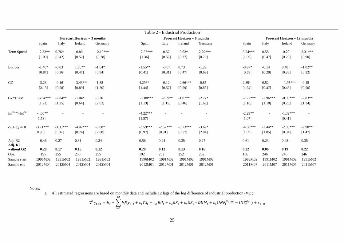
According to Table 2, the two standard measures of monetary policy, the term spread and the

real short-term interest rate, have predictive power for industrial production in two of the four

countries considered over the whole sample period. The term spread has a strong positive

effect on industrial production across all three forecasting horizons in Spain and Germany.

There is also an inverse relationship between real economic activity and the inflation adjusted

short-term rate in Spain and Germany, albeit the respective effect on industrial production

through the short-term real interest rate channel is weaker, both economically and

statistically, compared to the slope of the yield curve. For Italy and Ireland there is neither

econometric evidence of a positive relationship between the term spread and industrial

11

production nor evidence of an inverse relationship between the real rate of interest and

industrial production. The inflation differential relative to Germany exercises a sizeable

negative effect on industrial production across all three forecasting horizons in Spain and at

the 12-month horizon in Ireland.17

The marginal predictive effect of the credit spread on industrial production is captured by the

coefficients of GZ and GZ*DUM. The coefficient of the latter regressor captures the distinct

marginal effect of the GZ-spread during the Crisis period set off by the outbreak of the

Global Financial Crisis in August 2007 and lengthened by the Sovereign Debt Crisis in

Europe. Our empirical results suggest that increases in the GZ-spread proper predict lower

industrial production only in Ireland across all forecasting horizons prior to the Crisis period.

With the onset of the Global Financial Crisis, however, the negative effect of the GZ-spread

on industrial production is widely felt in Spain, Italy, and Ireland and Germany at the 12-

month forecasting horizon as evidenced by the negative and statistically significant

coefficient on GZ*DUM. The most compelling evidence for a significant change in the

predictive ability of the GZ-spread during the Crisis period is found in Spain where its

material effect on economic activity relative to the pre-Crisis period is evident at all

forecasting horizons. Indeed, the marginal impact of the spread in Spain is extreme: a one

percent increase in the spread predicts roughly a seven percent decline in the (annualized)

growth rate of industrial production.

To get a clearer picture of the overall predictive effect of the GZ-spread during the Crisis

period, we carry out a simple Wald test of the sum of the coefficients on the GZ-spread and

the interaction term. The sixth row of Table 2 reports the outcome of this test. The sum of the

coefficients on GZ and GZ*DUM is negative and statistically significant in the three

countries on the European periphery. This result holds at all forecasting horizons. The effects

of a widening credit spread are also apparent in Germany where a 100 basis increase in the

GZ-spread predicts an almost 3 per cent decline in the growth rate of industrial production at

the 12 month forecasting horizon. Indeed, three observations are noteworthy. First, the

economic significance of widening credit spreads during the Crisis period is remarkable with

the sum of the coefficients ranging from -2.44 to well over -4 in the countries on the

periphery. Thus, a widening of the GZ-spread by 100 basis points predicts a decrease of up to

4.5 percent in the growth rate of industrial production. Second, the economic significance of

17

The estimated coefficient on the relative inflation differential is reported only if it is statistically significant.

12

the GZ-spread is underscored further by a comparison of the goodness of fit measure in

forecasting equations with and without (in bold face) the GZ-spread. Comparing the entries

of rows seven and eight in Table 2, we find the adjusted R2 drops massively – often by 50

percent or more – if the GZ-spread is omitted from the forecasting equation. Third, in all

countries the credit spread appears to exercise a greater effect on the future growth rate of

industrial production than the standard measures of monetary policy.

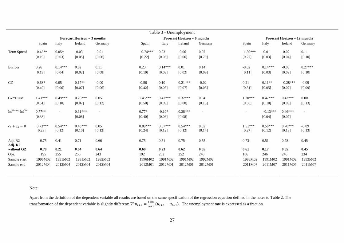
Table 3 summarizes the findings for the unemployment rate. Only in Spain is the term spread

an excellent predictor of changes in the unemployment rate across all three horizons. The

level of the real short-term money market rate reliably predicts future changes in the

unemployment rate in Italy at all forecasting horizons while it does so in Germany only at the

12-month horizon. Increases in the inflation differential are positively related to future

increases in the unemployment rate in Ireland at all three forecasting horizons but less so for

Spain where the inflation differential predicts future changes in the unemployment rate at the

3-month and marginally at the 6-month horizon. In Italy the effect of the inflation differential

on the rate of unemployment rate is strongly negative, particularly at the 12-month horizon.

This suggests the existence of a Phillips curve effect in Italy.

Just as in the case of industrial production, the GZ-spread appears to have exercised a

stronger effect on the rate of unemployment during the Crisis period. Increases in the GZ-

spread during the Crisis period predict higher unemployment rates in Spain, Italy, and Ireland

at all forecasting horizons: Wald tests of the significance of the sum of the coefficients on the

GZ-spread and GZ*DUM, reported in the sixth row, attest to the strong predictive ability of

the GZ-spread during the Crisis period. The marginal effect of the GZ-spread during the

Crisis period rises markedly in line with the length of the forecasting horizon in Spain,

peaking at 1.51 at the 12 month horizon. A similar pattern is observed in Ireland though the

marginal positive impact of credit spread increases on future unemployment rates during the

Crisis period is distinctly smaller, peaking at 0.70 at the 12-month horizon. In Italy the

marginal effect of the GZ-spread during the Crisis period stays relatively constant over the

three forecasting horizons, falling into the 0.5-0.6 range. There is no econometric evidence

that the GZ-spread has any predictive ability for the unemployment rate in Germany. Overall,

the economic significance of the GZ-spread as a driving factor of future changes in the rate of

unemployment is markedly weaker compared to industrial production. Only in Italy and in

Ireland at the 12-month horizon does the omission of the GZ-spread and its interaction term

result in a substantial drop in the goodness of fit of the forecasting equation.

13

The EMU-Period

The effective start of the Economic and Monetary Union in January 1999 transformed the

financial landscape of Europe. This date saw the introduction of the Euro and, importantly,

set in motion a process aiming at even closer financial integration of the European Union.

The purpose of this section is to examine whether the effect of the GZ-credit spread on

economic activity intensified as a result of the establishment of the EMU at the turn of the

millennium. Portugal now joins the list of countries for which this analysis is undertaken.

Inspection of Table 4 reveals that from 1999 to 2012 the predictive ability of equation (1) for

the growth rate of industrial production improves markedly only in Italy. The adjusted R2

rises substantially across all three forecasting horizons. Notice further that the sum of the

coefficients on the GZ-spread and the interaction term in Italy (reported in the sixth row)

more than doubles during the EMU period compared to the whole sample period. This result

holds at all forecasting horizons and underscores the extraordinary importance of the credit

spread as a predictor of future economic activity in Italy during the Crisis period since the

start of the currency union. For Portugal the results are less clear. On the one hand, there is

strong evidence of a connection between increases in the GZ-spread and future changes in

economic activity at the 6-month and 12-month horizon, particularly during the Crisis period.

On the other hand, the economic significance of the GZ-spread as a predictor appears to be

low as the adjusted R2 of the forecasting equation without the GZ-spread is about the same as

the one with it included. For the other countries, the economic significance of the GZ-spread

remains unscathed as the goodness of fit of the forecasting equation without the spread

decreases markedly.

We also observe notable changes in the transmission mechanism of monetary policy and the

predictive ability of the GZ-spread in more recent times. According to Table 4, changes have

been particularly acute in Germany. The results of the Wald test reported in row 6 suggest

that the credit spread exercises an immense effect on changes in industrial production at the

3-month horizon during the Crisis period; this effect wanes, however, both in terms of

economic and statistical significance as the forecasting horizon increases. What is interesting

about Germany (and Ireland) is that the forecasting ability of the GZ-credit spread at the 3-

month horizon is not limited to the Crisis period but holds throughout the EMU period. In

marked contrast, at the 12-month horizon the marginal effect of the GZ-spread on future

industrial production seems entirely confined to the Crisis period in Germany. Furthermore,

14

in Germany the interest rate channel also seems more potent while the term spread loses its

predictive power altogether during the EMU period.

Table 5 reports the results for the forecasting equation where the rate of unemployment is the

dependent variable. Again we observe that for Italy the predictive ability of the forecasting

equation is markedly better during the EMU period than over the whole sample period and

that the effect of the GZ-spread on future changes in the unemployment rate appears to be

stronger during the EMU period than before. Indeed in Italy movements in the GZ-spread

predict changes in the unemployment rate at the 3-month and 6-month horizon, respectively,

well before the start of the Crisis period; the effects of these movements in the GZ-spread on

future unemployment intensify during the Crisis period. In Portugal the results suggest that a

one percentage point increase in the credit spread during the Crisis period is associated with

roughly a one percentage point increase in the rate of unemployment at the 3-month and 6-

month horizon. For Germany we detect no systematic relationship between the GZ-spread

and the rate of unemployment during the EMU period. Overall, the economic significance of

the GZ-spread remains strong during the EMU period in Spain, Italy, Ireland and Portugal as

evidenced by the substantial decrease in the adjusted R2 of the forecasting equation without

the GZ-spread and the interaction term.

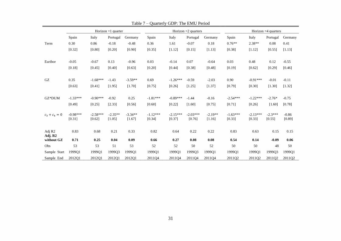
Quarterly Results

The marginal predictive effect of the GZ-spread is also tested on quarterly observations of

real GDP. Tables 6 and 7 present the econometric results for the whole sample period and the

EMU period, respectively. Overall, the findings of Table 6, which attest to a firm link

between the GZ-spread and the growth rate of GDP over 1, 2, and 4 quarters, amplify the

monthly results between the GZ-spread and industrial production. The GZ-spread predicts

future economic growth in Italy and Ireland.18

During the Crisis period the negative

predictive effect on future economic activity intensifies in Italy and Ireland and particularly

in Spain. In the latter country the negative impact effect on GDP growth of a rise in the GZ-

spread during the Crisis period increases in line with the forecasting horizon, peaking at

slightly over -1.85% for a 1% increase in the GZ-spread. In the three peripheral countries, the

effect of the GZ-spread on real GDP growth at different forecasting horizons falls between -1

and -2.3% during the Crisis period. For Germany there is no detectable link between the GZ

spread and real GDP growth.

18

The sample period for quarterly observations of real GDP in Ireland begins only in 1997.

15

Evidence of the importance of the GZ-spread during the shorter EMU period is found in all

countries.19

The effect of the GZ-spread on future real activity during the Crisis period is

undeniably strong at all three forecasting horizons in all five countries except Germany at the

four-quarter horizon: the sum-of-coefficients Wald tests reported in the fifth row of Table 7

clearly reject the null hypothesis that the GZ-spread during the Crisis period exercises no

effect on future GDP growth rates. However, there are slight differences across the countries

in the way the GZ-spread exercises the predicted negative effect on the growth rate of real

GDP. In Italy, for instance, the effect of the GZ-spread on real GDP ( ) predates the Crisis

period and its negative impact ( ) rises substantially during the Crisis period. In Spain,

the effect on real GDP growth materializes exclusively during the Crisis period. In Germany,

in contrast, the predictive ability of the GZ-spread at the one-quarter forecast horizon is

evident even before the onset of the Global Financial Crisis; there is no separate marginal

effect during the Crisis period.20

The economic significance of the GZ-spread and the

interaction term as predictors of future economic activity is impressive across the board.

Omitting both variables from the forecasting specification leads to a massive decrease in the

adjusted R2 for all countries but Spain at the one-quarter horizon where the decrease in the

predictive ability is only 12 percent. In Portugal, the GZ-spread and the interaction term are

the only variables that have predictive power over a four-quarter forecasting horizon.

Dropping both from the forecasting equation results in a negative adjusted R2!

VI. Conclusion

In February 2013, the annual yield on long-term (10-year) government bonds within the

EMU varied greatly. In the centre, the yield on German Bunds stood at 1.54 percent while on

the periphery yields were at least double the German yield (Ireland at 3.78 percent), thrice the

German yield (Italy at 4.49 percent, Spain at 5.22 percent), and more than fourfold the

German yield (Portugal at 6.40 percent).21

The dramatic difference in yields is due to

country-specific perceptions of risk and underscores the apparent fragmentation of European

public debt markets which has set in with the beginning of the Crisis period in 2007.

19

The results reported in Table 6 for the 1998:2-2011:12 period in Ireland are very similar to those obtained for

the slightly shorter EMU period. Hence the latter are not reported. 20

For Portugal, the standard errors of the coefficient estimates on the first differences of GZ and GZ*DUM are

highly inflated due to severe multicollinearity. The correlation coefficient for the two regressors is 0.95. A

similar problem, though less serious, applies to the standard errors estimated for Germany. The correlation

coefficient for GZ and GZ*DUM is 0.80 for Germany. 21

All data were retrieved from the Statistical Warehouse maintained by the European Central Bank. Table A1 in

the appendix gives an overview of yields on government bonds from 1993 to the recent past.

16

The current disruption of the European capital market must be put in perspective. In July

2007, before the outbreak of the Global Financial Crisis, the difference between the highest

yield on 10-year government bonds (Italy at 4.76 percent) and the lowest yield (Germany at

4.50 percent) was a paltry 26 basis points. In April 2012, at the conclusion of the sample

period of our study, the highest yield difference on the same instruments was a staggering

1018 basis points (Portugal at 12.01 percent and Germany at 1.83 percent).

In the countries on the European periphery, the adverse developments in the public debt

market have also spilled into the corporate debt market. Corporate bonds issued in these

countries have been saddled with a burdensome risk premium which derives largely from the

riskiness associated with domestic government debt.

In this paper we examine whether the pricing of risk is important for macroeconomic activity

at the country level. We design a risk-adjusted yield spread and test its predictive content for

economic activity on the periphery and the centre of Europe. The sample period runs from

1990 to 2012. Thus, the sample period is long enough to take account of distinctly different

epochs in recent European financial history. Capital markets in Europe were still very fairly

segmented and characterized by material borrowing cost differentials at the start of the 1990s.

The drive towards forming the EMU saw the eventual removal of all barriers to the free flow

of capital and the convergence of interest rates. The vision to create a single European capital

market first encountered problems with the outbreak of the Global Financial Crisis and was

dealt a severe blow when the Sovereign Debt Crisis created havoc in the capital markets on

the European periphery.

At the centre of our analysis is a risk-adjusted bond yield spread defined in a cross-country

context. Increases in the yield on corporate bonds issued in the countries on the periphery

relative to the riskless yield (calculated using German zero-coupon term structure data)

reflect the financial market’s unease about the future economic outlook in these countries.

The cross-country GZ-spread is a barometer of the risk premium that the financial market

imposes on borrowers. The risk premium rises in all countries during European-wide

recessions of the recent past, particularly those associated with the Global Financial and the

Sovereign Debt Crisis. Our findings indicate further that this GZ-type spread acts as a reliable

signal for imminent and near-term economic activity in the countries on the European

periphery whose financial markets were shaken to their foundations during the Crisis period.

The paper also employs the GZ-spread for forecasting purposes in a within-country context.

17

For Germany, the GZ-spread has predictive content for industrial production but not for the

unemployment rate. For GDP its predictive ability is confined to the EMU period.

18

References:

Ang, A., M. Piazzesi, and M. Wei, 2006, What does the yield curve tell us about GDP

Growth? Journal of Econometrics, 131, 359-403.

Bernanke, B. S., 1990, On the predictive power of interest rates and interest rate spreads, New

England Economic Review, November – December, 51-68.

Bernanke, B. S., and M. Gertler, 1995, Inside the black-box - the credit channel of monetary-

policy transmission, Journal of Economic Perspectives 9, 27-48.

Bernanke, B., M. Gertler, and S. Gilchrist, 1996, The financial accelerator and the flight to

quality, The Review of Economics and Statistics 78, 1-15.

Bernanke, B., M. Gertler, and S. Gilchrist, 1999, The financial accelerator in a quantitative

business cycle framework, in Handbook of Macroeconomics, vol. 1C, 1341-1393

(Amsterdam: Elsevier).

Bleaney, M. Mizen, and P. Veleanu, 2012, Credit spreads as predictors of economic activity

in eight european economies, mimeo, University of Nottingham.

Chan-Lau, J A. and I. V. Ivaschenko, 2001, Corporate bond risk and real activity: An

empirical analysis of yield spreads and their systematic components, International

Monetary Fund.

Davis, E. P., and G. Fagan, 1997, Are financial spreads useful indicators of future inflation

and output growth in eu countries?, Journal of Applied Econometrics 12, 701-714.

De Bondt, G., 2004, The balance sheet channel of monetary policy: First empirical evidence

for the euro area corporate bond market, International Journal of Finance &

Economics 9, 219-228.

Emery, K.M., 1996, The information content of the paper-bill spread, Journal of Economics

and Business 48, 1-10.

Estrella, Arturo, and G. Hardouvelis, 1991, The term structure as a predictor of real economic

activity, Journal of Finance 46, 555-576.

Financial Times, “European Company Borrowing Costs Rise,” November 30, 2010.

Financial Times, “Loan Rates Point to Eurozone Fractures,” September 3, 2012.

Friedman, B. and K. Kuttner, 1992, Money, income, prices, and interest rates, American

Economic Review 82, 472-492.

Gertler, M., and C. S. Lown, 1999, The information in the high-yield bond spread for the

business cycle: Evidence and some implications, Oxford Review of Economic Policy

15, 132-150.

19

Gilchrist, S., and E. Zakrajšek, 2012, Credit spreads and business cycle fluctuations,

American Economic Review 102, 1692-1720.

Harvey, C. R, 1988, The real term structure and consumption growth, Journal of Financial

Economics 22, 305-322.

King, T.B., A.T. Levin and R. Perli, 2007, Financial Market Perceptions of Recession Risks,

Finance and Economics Discussion Series 2007-57, Board of Governors of the

Federal Reserve System.

Mody, A., and M. P. Taylor, 2004, Financial predictors of real activity and the financial

accelerator, Economics Letters 82, 167-172.

Moersch, M., 1996, Predicting output with a money market spread, Journal of Economics

and Business 2, 185-200.

Mueller, Philippe, 2009, Credit spreads and real activity, (London School of Economics,

London).

Stock, J. H., and M. W. Watson, 2003, Forecasting output and inflation: The role of asset

prices, Journal of Economic Literature 41, 788-829.

Wall Street Journal, “Bonds with Banks Fraying,” April 10, 2012.

Corresponding Author: Alfred V Guender ([email protected]), Dept. of

Economics and Finance, University of Canterbury, Private Bag 4800, Christchurch, NZ.

Phone: 64-3-364-2519.

mailto:[email protected]

20

Figure 1: The GZ-Spread in Europe

Note: The shaded areas represent European-wide recessions.

0

1

2

3

4

5

6

7

8

%

90 92 94 96 98 00 02 04 06 08 10 12

S P A I N

0

1

2

3

4

5

6

7

8

%

90 92 94 96 98 00 02 04 06 08 10 12

I T A L Y

21

0

2

4

6

8

10

%

90 92 94 96 98 00 02 04 06 08 10 12

I R E L A N D

0

2

4

6

8

10

%

90 92 94 96 98 00 02 04 06 08 10 12

P O R T U G A L

22

0

1

2

3

4

5

%

90 92 94 96 98 00 02 04 06 08 10 12

G E R M A N Y

23

Table 1A: Summary Statistics

Spain Italy Germany Portugal Ireland

Mean No. of bonds per firm 4.61 4.32 5.29 3.00 4.69

Standard deviation 4.30 6.91 6.97 4.24 7.89

Min No. of bonds per firm 1.00 1.00 1.00 1.00 1.00

Max No. of bonds per firm 16.00 37.00 35.00 13.00 30.00

Total number of bonds 75 174 330 42 59

Total number of observations 4,085 8,251 14,953 1,781 2,938

Total number of issuing firms 17 41 62 13 13

Mean maturity at issue (yrs.) 11.81 8.37 6.93 7.1 12.76

Standard deviation 8.94 6.14 4.1 4.72 11.37

Mean coupon 5.45% 5.79% 5.35% 5.46% 10.74%

Standard deviation 1.73% 1.79% 1.94% 1.09% 24.49%

Mean yield 4.93% 5.59% 4.56% 5.68% 8.10%

Standard deviation 1.63% 2.54% 2.17% 2.43% 5.64%

Median bond credit rating

(S&P) BBB BBB BBB+ BB+ A

Series start (all end 2012M08) 1996M02 1990M01 1990M03 1999M04 1990M01

Notes:

1. Bond rating data was not available for all bonds. Where it was available, the most recent rating

for the bond (rather than the firm) is reported.

2. ‘Total number of observations’ refers to the total number of spreads in each country.

24

Table 1B: Summary Statistics for GZ-Spread

1B.1 Whole Sample Period

Spain Italy Ireland Germany

Mean 1.58 2.73 4.13 1.72

Maximum 6.16 7.54 9.50 4.93

Minimum 0.36 0.39 0.85 0.16

Std. Deviation 1.12 1.53 2.29 0.89

Observations 199 272 272 270

Sample Period 1996:02-2012:08 1990:01-2012:08 1990:01-2012:08 1990:03-2012:08

1B.2 The Pre-EMU Period


Mean 1.72 3.55 4.63 1.50

Maximum 3.99 7.54 9.37 4.93

Minimum 0.79 0.39 1.12 0.16

Std. Deviation 0.73 1.70 2.60 1.18

Observations 35 108 108 106

Sample Period 1996:02-1998:12 1990:01-1998:12 1990:01-1998:12 1990:03-1998:12

1B.3 The EMU Period (1999:01-2012:08)

Spain Italy Ireland Portugal* Germany

Mean 1.55 2.19 3.80 1.99 1.87

Maximum 6.16 5.68 9.50 9.53 4.25

Minimum 0.36 0.42 0.85 0.17 0.93

Std. Deviation 1.18 1.12 2.00 2.10 0.59

Observations 164 164 164 161 164

1B.4 The Pre-Crisis Period (1999:01-2007:07)

Spain Italy Ireland Portugal* Germany

Mean 0.88 1.77 2.57 0.86 1.57

Maximum 1.64 4.55 5.87 1.69 2.41

Minimum 0.36 0.42 0.85 0.17 0.93

Std. Deviation 0.28 0.88 1.16 0.37 0.34

Observations 103 103 103 100 103

1B.5 The Crisis Period (2007:08-2012:08)

Spain Italy Ireland Portugal Germany

Mean 2.68 2.89 5.87 3.85 2.37

Maximum 6.16 5.68 9.50 9.53 4.25

Minimum 0.72 1.17 3.44 1.11 1.51

Std. Deviation 1.26 1.13 1.28 2.42 0.59

Observations 61 61 61 61 61

*Sample Period begins in 1999:04

25

Table 2 - Industrial Production

Forecast Horizon = 3 months






Term Spread 2.32** 0.76* -0.80 2.19***

2.57*** 0.57 -0.62* 2.29***

3.54*** 0.58 -0.29 2.31***

[1.00] [0.42] [0.52] [0.78]

[1.36] [0.52] [0.37] [0.79]

[1.09] [0.47] [0.29] [0.90]

Euribor -1.46* -0.03 1.05** -1.64* -1.55** -0.07 0.73 -1.29 -0.97* -0.14 0.48 -1.02**

[0.87] [0.36] [0.47] [0.94] [0.41] [0.31] [0.47] [0.69] [0.59] [0.29] [0.36] [0.52]

GZ 3.23 -0.16 -3.43*** -1.88 4.29** 0.12 -2.66*** -0.85 2.89* 0.52 -1.95*** -0.15

[2.15] [0.58] [0.89] [1.30] [1.44] [0.57] [0.59] [0.83] [1.64] [0.47] [0.43] [0.50]

GZ*DUM -6.94*** -2.84** -1.04* -3.20 -7.88*** -2.69** -1.07** -2.77* -7.27*** -2.96*** -0.95*** -2.83**

[1.23] [1.25] [0.64] [2.03] [1.19] [1.15] [0.46] [1.69] [1.18] [1.18] [0.28] [1.34]

InfHome-InfGer -4.06** - - - -4.22*** - - - -2.29** - -1.32*** - [1.73] [1.57] [1.07] [0.41]

-3.71*** -3.00*** -4.47*** -5.08* -3.59*** -2.57*** -3.73*** -3.62*

-4.38*** -2.44** -2.90*** -2.98**

[0.95] [1.07] [0.74] [2.88] [0.97] [0.91] [0.57] [2.04] [1.09] [1.05] [0.34] [1.47]

Adj. R2 0.46 0.27 0.31 0.24 0.56 0.24 0.35 0.27 0.61 0.23 0.48 0.35

Adj. R2

without GZ 0.29 0.17 0.15 0.12 0.28 0.12 0.13 0.16 0.22 0.06 0.19 0.22

Obs. 195 255 255 255 192 252 252 252 186 246 246 246

Sample start 1996M02 1991M02 1991M02 1991M02 1996M02 1991M02 1991M02 1991M02 1996M02 1991M02 1991M02 1991M02

Sample end 2012M04 2012M04 2012M04 2012M04 2012M01 2012M01 2012M01 2012M01 2011M07 2011M07 2011M07 2011M07

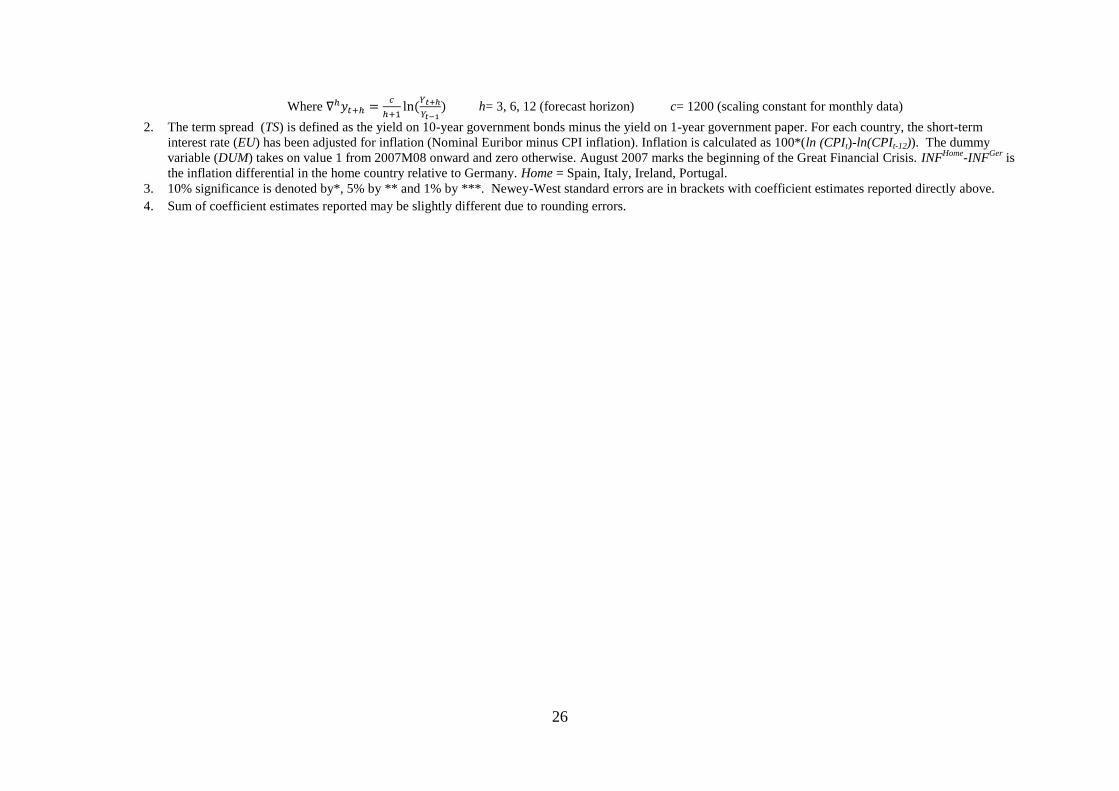
Notes:

1. All estimated regressions are based on monthly data and include 12 lags of the log difference of industrial production ( ):

∑

(

)

26

Where

(

) h= 3, 6, 12 (forecast horizon) c= 1200 (scaling constant for monthly data)

2. The term spread (TS) is defined as the yield on 10-year government bonds minus the yield on 1-year government paper. For each country, the short-term

interest rate (EU) has been adjusted for inflation (Nominal Euribor minus CPI inflation). Inflation is calculated as 100*(ln (CPIt)-ln(CPIt-12)). The dummy

variable (DUM) takes on value 1 from 2007M08 onward and zero otherwise. August 2007 marks the beginning of the Great Financial Crisis. INFHome

-INFGer

is

the inflation differential in the home country relative to Germany. Home = Spain, Italy, Ireland, Portugal.

3. 10% significance is denoted by*, 5% by ** and 1% by ***. Newey-West standard errors are in brackets with coefficient estimates reported directly above.

4. Sum of coefficient estimates reported may be slightly different due to rounding errors.

27

Table 3 - Unemployment







Term Spread -0.43** 0.05* -0.03 -0.01

-0.74*** 0.03 -0.06 0.02

-1.30*** -0.01 -0.02 0.11

[0.19] [0.03] [0.05] [0.06]

[0.22] [0.03] [0.06] [0.79]

[0.27] [0.03] [0.04] [0.10]

Euribor 0.26 0.14*** 0.02 0.11 0.23 0.14*** 0.01 0.14 -0.02 0.14*** -0.00 0.27***

[0.19] [0.04] [0.02] [0.08] [0.19] [0.03] [0.02] [0.09] [0.11] [0.03] [0.02] [0.10]

GZ -0.68* 0.05 0.17** -0.00 -0.56 0.10 0.21*** -0.02 0.21 0.11** 0.28*** -0.09

[0.40] [0.06] [0.07] [0.06] [0.42] [0.06] [0.07] [0.08] [0.31] [0.05] [0.07] [0.09]

GZ*DUM 1.41*** 0.49*** 0.26*** 0.05 1.45*** 0.47*** 0.32*** 0.04 1.30*** 0.47*** 0.42*** 0.00

[0.51] [0.10] [0.07] [0.12] [0.50] [0.09] [0.08] [0.13] [0.36] [0.10] [0.09] [0.13]

InfHome-InfGer 0.77** - 0.31*** - 0.77* -0.10*

0.38*** - - -0.13*** 0.46*** -

[0.38] [0.08] [0.40] [0.06] [0.08] [0.04] [0.07]

0.73***

[0.23]

0.54***

[0.12]

0.43***

[0.10]

0.05

[0.12]

0.89***

[0.24]

0.57***

[0.12]

0.54***

[0.12]

0.02

[0.14]

1.51***

[0.27]

0.58***

[0.12]

0.70***

[0.13]

-0.09

[0.13]

Adj. R2 0.75 0.41 0.71 0.66 0.75 0.51 0.75 0.55 0.73 0.51 0.78 0.45

Adj. R2

without GZ 0.70 0.21 0.64 0.64 0.68 0.23 0.62 0.55 0.61 0.17 0.55 0.45

Obs. 195 255 255 243 192 252 252 240 186 246 246 234

Sample start 1996M02 1991M02 1991M02 1992M02 1996M02 1991M02 1991M02 1992M02 1996M02 1991M02 1991M02 1992M02

Sample end 2012M04 2012M04 2012M04 2012M04 2012M01 2012M01 2012M01 2012M01 2011M07 2011M07 2011M07 2011M07

Note:

Apart from the definition of the dependent variable all results are based on the same specification of the regression equation defined in the notes to Table 2. The

transformation of the dependent variable is slightly different:

( ). The unemployment rate is expressed as a fraction.

28

Table 4 - Industrial Production: The EMU Period







Term Spread 2.52** 2.43 -0.08 0.75 0.99

3.28*** 4.55 -0.30 0.49 1.73

3.91*** 7.06** -0.05 0.33 2.02

[1.32] [2.75] [0.92] [0.60] [1.10]

[1.34] [3.20] [0.77] [0.42] [1.09]

[1.41] [3.24] [0.47] [0.35] [0.90]

Euribor -1.25 -2.72 0.58 -1.14 -4.00** -0.71 -0.97 1.14 -0.85 -3.33** -0.56 1.14 1.89*** -0.47 -2.79***

[1.03] [1.77] [1.18] [1.21] [1.93] [0.87] [1.51] [0.81] [0.72] [1.46] [0.71] [1.59] [0.36] [0.56] [0.72]

GZ 5.28* -4.51*** -5.25*** 5.21 -10.26*** 8.35*** -3.10*** -3.49*** 1.89 -3.49 7.16** -1.87*** -2.86*** 1.71 0.62

[3.18] [0.58] [1.90] [3.65] [4.08] [3.19] [0.88] [1.41] [1.76] [2.93] [3.21] [0.59] [0.59] [1.31] [2.22]

GZ*DUM -8.60*** -2.36** 0.20 -10.66** -0.96 -10.77*** -2.31** -0.25 -6.40*** -2.52 -9.93*** -3.13*** -0.14 -5.63*** -3.60**

[3.08] [1.05] [1.02] [5.35] [1.74] [2.98] [1.08] [0.74] [2.62] [2.18] [2.81] [1.01] [0.35] [1.97] [1.74]

InfHome-InfGer -5.39*** - - - - -5.48*** - - - -2.72* - - - - [2.18] [1.87] [1.45]

-3.31***

[1.06]

-6.87***

[1.87]

-5.05***

[1.20]

-5.45

[3.81]

-11.22***

[4.48]

-2.42***

[0.90]

-5.41***

[1.41]

-3.74***

[0.89]

-4.51***

[1.87]

-6.01**

[2.69]

-2.77***

[1.00]

-5.01***

[1.14]

-3.00***

[0.39]

-3.92***

[1.53]

-2.98*

[1.65]

Adj. R2 0.46 0.41 0.37 0.23 0.33 0.57 0.38 0.39 0.12 0.28 0.60 0.46 0.54 0.06 0.38

Adj. R2

without GZ 0.27 0.17 0.24 0.18 0.09 0.27 0.16 0.24 0.12 0.11 0.21 0.13 0.20 0.05 0.18

Obs. 160 160 160 156 160 157 157 157 153 157 151 151 151 147 151

Sample start 1999M01 1999M01 1999M01 1999M05 1999M01 1999M01 1999M01 1999M01 1999M05 1999M01 1999M01 1999M01 1999M01 1999M05 1999M01

Sample end 2012M04 2012M04 2012M04 2012M04 2012M04 2012M01 2012M01 2012M01 2012M01 2012M01 2011M07 2011M07 2011M07 2011M07 2011M07

Notes: See notes to Table 1.

1. For Portugal the GZ variable has been differenced to make it stationary.

29

Table 5 - Unemployment: The EMU Period







Term Spread -0.58*** 0.09 -0.03 -0.20** 0.05

-1.27*** 0.10 -0.19* -0.22*** 0.01

-1.67*** -0.21 -0.07 -0.28*** 0.07

[0.23] [0.14] [0.05] [0.09] [0.08]

[0.38] [0.12] [0.11] [0.84] [0.10]

[0.32] [0.17] [0.12] [0.05] [0.16]

Euribor 0.22 0.03 0.02 0.09 0.09 -0.16 -0.00 0.02 0.06 0.14 -0.16 -0.23 0.01 -0.02 0.29**

[0.25] [0.13] [0.02] [0.14] [0.10] [0.18] [0.12] [0.17] [0.13] [0.13] [0.18] [0.17] [0.18] [0.09] [0.14]

GZ -1.05* 0.28*** 0.17** 0.43 0.38* -0.81 0.22** 0.19* 0.48 0.15 -1.08 0.12 0.29*** 0.10 -0.35

[0.55] [0.10] [0.07] [0.44] [0.23] [0.56 [0.10] [0.11] [0.39] [0.26] [0.67] [0.11] [0.10] [0.32] [0.28]

GZ*DUM 1.69*** 0.45*** 0.26*** 0.59 -0.13 1.38*** 0.49*** 0.38*** 0.45 -0.02 2.10*** 0.65*** 0.45*** 0.36 0.15

[0.58] [0.11] [0.07] [0.49] [0.15] [0.42] [0.11] [0.10] [0.43] [0.19] [0.54] [0.13] [0.11] [0.42] [0.21]

InfHome-InfGer - -0.34** 0.31*** - - - -0.36*** 0.44*** - - - -0.28* 0.45*** - - [0.15] [0.08] [0.12] [0.16] [0.16] [0.16]

0.64***

[0.26]

0.73***

[0.10]

0.43***

[0.10]

1.02***

[0.36]

0.24

[0.20]

0.57**

[0.29]

0.71***

[0.09]

0.57***

[0.13]

0.93***

[0.29]

0.13

[0,22]

1.01***

[0.28]

0.77***

[0.10]

0.74***

[0.14]

0.46

[0.35]

-0.20

[0.21]

Adj. R2 0.74 0.62 0.71 0.33 0.58 0.74 0.69 0.70 0.34 0.46 0.77 0.66 0.76 0.28 0.35

Adj. R2

without GZ 0.68 0.33 0.54 0.24 0.57 0.67 0.37 0.51 0.23 0.46 0.61 0.15 0.40 0.11 0.34

Obs. 160 160 160 156 160 157 157 157 153 157 151 151 151 147 151

Sample start 1999M01 1999M01 1999M01 1999M05 1999M01 1999M01 1999M01 1999M01 1999M05 1999M01 1999M01 1999M01 1999M01 1999M05 1999M01

Sample end 2012M04 2012M04 2012M04 2012M04 2012M04 2012M01 2012M01 2012M01 2012M01 2012M01 2011M07 2011M07 2011M07 2011M07 2011M07

30

Note: All estimated regressions are based on quarterly data and include 4 lags of the log difference of real GDP ( ):

∑

(

)

where

(

) h= 1, 2, 4 (forecast horizon) c= 400 (scaling constant for quarterly data)

Table 6 – Quarterly GDP

Horizon =1 quarter

Horizon =2 quarters

Horizon =4 quarters




Term 0.22 1.10** -0.68 -0.02

0.31 1.29* -0.16 0.17

0.75** 1.43** 0.26 0.20

[0.25] [0.57] [0.62] [0.39]

[0.28] [0.69] [0.52] [0.35]

[0.35] [0.67] [0.24] [0.35]

Euribor -0.26 0.26 -0.24 -0.91*

-0.24 0.32 -0.05 -0.74**

-0.14 0.39* 0.46 -0.59**

[0.18] [0.20] [0.39] [0.5]

[0.20] [0.22] [0.34] [0.37]

[0.22] [0.22] [0.35] [0.28]

GZ 0.61 -0.48** -1.52*** -0.20

0.73 -0.41* -0.92* 0.13

0.86 -0.37** -0.94*** 0.36

[0.45] [0.16] [0.61] [0.59]

[0.55] [0.21] [0.48] [0.41]

[0.62] [0.17] [0.34] [0.27]

GZ*DUM -1.71*** -1.13*** -0.81** -1.09

-2.00*** -1.15*** -1.04*** -1.01

2.54*** -1.42*** -1.03*** -0.95*

[0.48] [0.42] [0.38] [0.76]

[0.58] [0.35] [0.30] [0.66]

[0.62] [0.33] [0.24] [0.53]

InfHome-InfGer -0.71* - -0.97* -

-0.75* - -0.91** -

- - -0.71*** -

[0.39] [0.56]

[0.46] [0.40]

[0.26]

-1.10***

[0.22]

-1.61***

[0.48]

-2.33***

[0.40]

-1.29

[1.00]

-1.27***

[0.24]

-1.56***

[0.40]

-1.96***

[0.32]

-0.89

[0.73]

-1.85***

[0.39]

-1.79***

[0.35]

-1.97***

[0.21]

-0.59

[0.52]

Adj. R2 0.85 0.53 0.52 0.20

0.85 0.53 0.63 0.20

0.84 0.50

0.84 0.21

Adj. R2

without GZ 0.73 0.22 0.24 0.08 0.68 0.20 0.33 0.09 0.59 0.06 0.43 0.09

Obs 64 80 56 80

63 79 55 79

61 77 53 77

Sample Start 1996Q2 1992Q2 1998Q2 1992Q2

1996Q2 1992Q2 1998Q2 1992Q2

1996Q2 1992Q2 1998Q2 1992Q2

Sample End 2012Q1 2012Q1 2012Q1 2012Q1

2011Q4 2011Q4 2011Q4 2011Q4

2011Q2 2011Q2 2011Q2 2011Q2

31

Table 7 – Quarterly GDP: The EMU Period

Horizon =1 quarter

Horizon =2 quarters

Horizon =4 quarters

Spain Italy Portugal Germany



Term 0.30 0.86 -0.18 -0.48

0.36 1.61 -0.07 0.18

0.76** 2.38** 0.08 0.41

[0.32] [0.80] [0.20] [0.90]

[0.35] [1.12] [0.15] [1.13]

[0.38] [1.12] [0.55] [1.13]

Euribor -0.05 -0.67 0.13 -0.96

0.03 -0.14 0.07 -0.64

0.03 0.48 0.12 -0.55

[0.18] [0.45] [0.40] [0.63]

[0.20] [0.44] [0.38] [0.48]

[0.19] [0.62] [0.29] [0.46]

GZ 0.35 -1.68*** -1.43 -3.59**

0.69 -1.26*** -0.59 -2.03

0.90 -0.91*** -0.01 -0.11

[0.63] [0.41] [1.95] [1.70]

[0.75] [0.26] [1.25] [1.37]

[0.79] [0.30] [1.30] [1.32]

GZ*DUM -1.33*** -0.90*** -0.92 0.25

-1.81*** -0.89*** -1.44 -0.16

-2.54*** -1.22*** -2.76* -0.75

[0.49] [0.25] [2.33] [0.56]

[0.60] [0.22] [1.60] [0.75]

[0.71] [0.26] [1.60] [0.78]

-0.98***

[0.31]

-2.58***

[0.62]

-2.35**

[1.05]

-3.34**

[1.67]

-1.12***

[0.34]

-2.15***

[0.37]

-2.03***

[0.76]

-2.19**

[1.16]

-1.63***

[0.33]

-2.13***

[0.33]

-2.3***

[0.55]

-0.86

[0.89]

Adj R2 0.83 0.68

0.21 0.33

0.82 0.64 0.22 0.22

0.83

0.63 0.15 0.15

Adj. R2

without GZ 0.71 0.25 0.04 0.09 0.66 0.27 0.08 0.08 0.54 0.14 -0.09 0.06

Obs 53 53 51 53

52 52 50 52

50 50 48 50

Sample Start 1999Q1 1999Q1 1999Q3 1999Q1

1999Q1 1999Q1 1999Q3 1999Q1

1999Q1 1999Q1 1999Q3 1999Q1

Sample End 2012Q1 2012Q1 2012Q1 2012Q1

2011Q4 2011Q4 2011Q4 2011Q4

2011Q2 2011Q2 2011Q2 2011Q2

32

Appendix:

Table A1: Yields (%) on 10-yr Government Bonds

Date Germany Italy Spain Portugal Ireland

February 2013 1.54 4.49 5.22 6.40 3.78

April 2012 1.83 5.68 5.79 12.01 6.88

July 2007 4.50 4.76 4.60 4.73 4.59

January 1999 3.70 3.92 3.88 3.90 3.89

January 1993 7.15 13.43 12.16 10.67 (July) 9.88

33

Variable Code Description Raw units Frequency Transformation Source

Industrial Production IP or Y Total industrial production index. Seasonally

and working day adjusted.

Index (base year =

2005)

Monthly The log difference over

one period or log-

difference over h-periods.

OECD

GDP GDP or Y This is real GDP. Seasonally and working day

adjusted

Millions of Euro

(2000 market

prices)

Quarterly The log difference over

one period or log-

difference over h-periods

when used as dependant

variable (see equation (1))

EuroStat

Unemployment U Total Unemployment rate. Seasonally

adjusted.

Percentage points Monthly None OECD

GZ spread GZ Spread is constructed from yields on bond

securities and risk-free rate (below). The

yield to redemption on each bond is

calculated by DataStream.

Percentage points Monthly None DataStream and own

calculations

Risk-free rate rf We construct a German government yield

curve from zero rates provided by the

German Bundesbank and interpolate. See text

for more details.

Percentage points Monthly Not-transformed. Used to

calculate the GZ spread

German Bundesbank

Inflation CPI CPI all products. Not seasonally adjusted. Index Monthly Transformed into log-

difference over one year.

DataStream

Short term rate

(nominal)

EU Short term rate provided by the OECD. It

consists of different rates over time. It is the

Euribor interbank rate after 2000. Prior to

that it is the shortest maturity government

bond yield.

Percentage points Monthly None OECD

Term spread TS Difference between long and short end of

DataStream-calculated yield curve.

Percentage points Monthly None DataStream and own

calculations

Table A2: Data Description and Sources

34

Short Abstract:

This paper examines whether information from bond markets provides a reliable signal for

future economic activity in Europe. The inclusion of a risk-adjusted bond yield spread

improves markedly the goodness of fit of the forecasting equation for economic activity in

four countries on the European periphery. The within-sample forecasting ability of the GZ-

spread is remarkable, both over the whole sample period and a sub-sample period marking

the effective beginning of the EMU in Europe. Its effect on economic activity is felt

particularly during the 2007-12 Crisis period. For Germany the predictive ability of the GZ-

spread is less impressive.

Longer Abstract:

In this paper we examine whether the pricing of risk is important for macroeconomic activity

at the country level. We design a risk-adjusted yield spread and test its predictive content for

economic activity on the periphery and the centre of Europe over the 1990-2012 period. At

the centre of our analysis is a risk-adjusted bond yield spread defined in a cross-country

context. Increases in the yield on corporate bonds issued in the countries on the periphery

relative to the riskless yield (calculated using German zero-coupon term structure data)

reflect the financial market’s unease about the future economic outlook in these countries.

The cross-country GZ-spread is a barometer of the risk premium that the financial market

imposes on borrowers. The risk premium rises in all countries during European-wide

recessions of the recent past, particularly those associated with the Global Financial and the

Sovereign Debt Crisis. Our findings indicate further that this GZ-type spread acts as a reliable

signal for imminent and near-term economic activity in countries where financial markets

were shaken to their foundations during the Crisis period. For Germany, the GZ-spread has

predictive content for industrial production but not for the unemployment rate. For GDP its

predictive ability is confined to the EMU period.

the centre matters for the periphery of europe: the

Documents