See discussions, stats, and author profiles for this publication at: https://www.researchgate.net/publication/267256791

The Causes of Increase in Homeownership in the 1990s

Article

CITATIONS

2

READS

10

2 authors, including:

Stuart Gabriel

University of California, Los Angeles

121 PUBLICATIONS   2,313 CITATIONS   

SEE PROFILE

All content following this page was uploaded by Stuart Gabriel on 11 December 2014.

The user has requested enhancement of the downloaded file.

The Causes of Increase in Homeownership in the 1990s

Stuart A. Gabriel

Department of Finance and Business Economics and Lusk Center for Real Estate

Marshall School of Business University of Southern California

Stuart S. Rosenthal

Department of EconomicsCenter for Policy Research

Syracuse University

Working Paper No. 03-01

Research Institute for Housing AmericaBOARD OF TRUSTEES

Stephen B. Ashley, CMBS.B. Ashley Management Corporation

Michael Petrie, CMBP/R Mortgage & Investment Company

Teresa Bryce, Esq.Nexstar Financial Corporation

Gary J. KallsenThrivent Financial for Lutherans

R. Glenn WertheimCharter Mortgage Company

James W. Nelson, CMBPast President, Mortgage Bankers Association

STAFFDouglas G. Duncan, Ph.D.

Senior Vice President, Research and Business DevelopmentChief Economist

Mortgage Bankers Association

James L. Freund, Ph.D.Director

Mortgage Bankers Association

The Causes of Increase in Homeownership in the 1990s

Stuart A. Gabriel

Department of Finance and Business Economics and Lusk Center for Real Estate

Marshall School of Business University of Southern California

Stuart S. Rosenthal

Department of EconomicsCenter for Policy Research

Syracuse University

Working Paper No. 03-01

October 2003

The authors thank Jim Freund and seminar participants at the Federal Reserve Bank of Philadelphia for helpful comments. Any remaining errors are our own.

© Research Institute for Housing America 2003. All rights resevered.

1

I. Introduction

U.S. homeownership rates moved up substantially over the course of the 1990s to reach a

historic high of nearly 67.5 percent in 2001. This increase in homeownership coincided with

several important changes in the U.S. economy, including shifts in the demographic composition

of the population, innovations in mortgage finance, the economic boom of the 1990s, and

declining interest rates. An important goal of this paper is to shed light on the degree to which

these and related factors have contributed to the rise in homeownership.

The past decade also has witnessed heightened concern regarding the persistently low

levels of homeownership evidenced among minority and underserved populations. In part, the

debate has focused on racial disparities in economic status that contribute to large gaps in

homeownership between white and non-white households.1 In addition, prominent newspaper

accounts and an influential study by the Federal Reserve Bank of Boston have heightened

concerns regarding systematic and unfair denial of mortgage credit to minorities. (Munnell et al

(1996))2,3. Partly in response to these concerns, a variety of new mortgage products and

programs were introduced in the 1990s with the intent of improving access to owner-occupied

housing, especially among underserved and minority households.4 A related goal of this paper is

1See, for example, Wachter and Megbolugbe (1992), Gyourko and Linneman (1996), Coulson (1999), and Gabriel and Painter (2003). 2In May 1988, the Atlanta Constitution published a four part series, “The Color of Money,” while the Detroit Free Press published a similar series in July 1988. Those and like analyses of Home Mortgage Disclosure Act (HMDA) data showed that mortgage application rejection rates for African Americans in 1990 were about 2-1/2 times larger than those for white households with similar income (see Canner and Smith (1991) for details on the HMDA data). 3Beginning in 1990, lenders were required by HMDA to report the location of residential loans made along with the income, race, and gender of loan applicants and whether the loan application was withdrawn (by the applicant), approved, or denied. See Rehm (1991a, 1991b) and Munnell et. al. (1996) for further discussion of the HMDA data. 4For example, Zero DownTM is an affordable mortgage product newly offered by Bank of America that is now available in numerous states. It is a is a conventional mortgage that requires zero downpayment. In addition, closing costs can come from a gift, the seller, or can be financed (see Bank of America (1998)).

2

to ascertain the extent to which credit barriers have restricted access to homeownership. Further,

we seek to evaluate how the influence of credit barriers has changed over the course of recent

decades.

We begin with summary measures. Table 1 displays homeownership rates in the United

States for select years over the 1983 to 2001 period based on data from the Survey of Consumer

Finances, weighted so as to be representative of the U. S. population. Our sample includes all

households except for those that report household income that is negative, above $500,000 (in

2001 dollars), or missing. Also, both here and throughout the paper, our measure of

homeownership treats mobile home residents that own any portion of their home (land or

structure) as owner-occupiers.5

As evidenced in Table 1, homeownership rates for the sampled population edged up 1

percentage point from 1983 to 1989, and then rose a further 3.5 percentage points over the

subsequent twelve years to reach 67.3 percent in 2001.6 While the increase in homeownership

occurred among white, black and Hispanic households, it was especially pronounced for African

Americans, rising 5.1 percent points over the 1989 to 2001 period. What these changes do not

capture, however, is that the homeownership rate gap between white and minority households

largely persisted over this period. To be precise, in 2001, the white-black and white-Hispanic

gaps in homeownership rates stood at 26.2 and 29.5 percentage points, respectively. That

disparity has gained attention at the highest political levels, including recent statements by

5When the omitted households are included in the sample our estimates of homeownership rates match exactly those reported by Kennickel (1999) in his comparison of homeownership rates in the SCF to the CPS for the years 1989, 1992, 1995, and 1998. 6This rise is consistent with widely reported increases in homeownership rates during the 1990s.See estimates based on the Consumer Population Survey (CPS) and the Decennial Census at the Census website, for example: http://www.census.gov/hhes/www/housing/hvs/q103tab5.html .

3

President Bush and his related call for at least 5.5 million additional minority homeowners by

2010:7

“The goal is, everybody who wants to own a home has got a shot at doing so. The problem is we have what we call a homeownership gap in America. Three-quarters of Anglos own their homes, and yet less than 50 percent of African Americans and Hispanics own homes. That ownership gap signals that something might be wrong in the land of plenty. And we need to do something about it.” President George Bush, June 18, 2002, http://www.whitehouse.gov/news/releases/2002/06/20020618-1.html.

The bottom panel of Table 1 reports information pertaining to whether households are

currently saving to purchase a home.8 This information is new to the literature and may indicate

recent evolution in factors that might contribute to a rise in minority homeownership and to a

related narrowing of racial gaps in homeownership. Findings are plotted in Figure 1 to facilitate

review.

As evidenced in Figure 1, the fraction of black and Hispanic renters saving to purchase a

home rose sharply over the past few decades to levels equal to or in excess of those recorded for

white renters. 9 Those results stand in marked contrast to findings for earlier periods; in 1983, for

7The following White House Press Release announced President Bush’s goal of increasing the number of minority homeowners by at least 5.5 million by 2010: “Today, President Bush announced a new goal to help increase the number of minority homeowners by at least 5.5 million before the end of the decade. The President's aggressive housing agenda will help dismantle the barriers to homeownership by providing down payment assistance, increasing the supply of affordable homes, increasing support for self-help homeownership programs, and simplifying the home buying process & increasing education. The President also issued "America's Homeownership Challenge" to the real estate and mortgage finance industries to join in his effort to increase the number of minority homeowners by taking concrete steps to tear down the barriers to homeownership that face minority families.” Source: White House Press Release, June 17, 2002 http://www.whitehouse.gov/news/releases/2002/06/20020617.html 8For each survey year, we characterized a family as saving to purchase a home if either their first or second most important reason for saving was for future home purchase. 9Two recent papers yield complementary results that are suggestive of a narrowing of longstanding racial gaps in homeownership rates. The first, by Painter, Gabriel, and Myers (2001), examined Los Angeles data from 1980 and 1990 and found that household attributes fully explain homeownership gaps between white, Asian, and Hispanic households although a large gap between White and African American homeownership rates remains. The second, by Rosenthal (2002), examined 1998 SCF data for the United States and found that renter expectations of buying a home were remarkably similar across race, both in the raw data and even after controlling for household attributes.

4

instance, only 6.8 percent of blacks and 8.5 percent of Hispanics were savings to purchase a

home, compared with some 12.4 percent of white households. Not surprisingly, few

homeowners indicate that they are saving to purchase a home.

The increased rate of minority savings behavior is suggestive that something has changed

that has affected expectations of future homeownership among minority households. One

obvious possibility is the introduction of new mortgage designs and related initiatives in the

1990s that sought to enhance mortgage loan origination among minority and underserved

populations. But the early 1990s also marked the beginning of an economic boom that lasted

through the remainder of the decade. Enhanced access to high quality jobs and related

improvements in minority economic well-being also may have contributed to the increase in

minority savings activity.

It is tempting to speculate about the implications of elevated minority home savings rates

for future minority homeownership. For example, has the increase in minority savings for home

purchase been matched by an increase in minority demand for homeownership, suggesting an

anticipated narrowing in persistent racial disparities in homeownership? To address this and

related questions, as pertain to both minority and non-minority groups, we decompose changes in

actual homeownership rates over the 1983 to 2001 period into three broad sets of determinants:

changes in the demand for homeownership holding constant household attributes, changes in the

demand for homeownership arising from changes in household economic and demographic

characteristics, and changes in the influence of credit barriers.10

Several findings stand out. First, for the sample overall, credit barriers reduced observed

homeownership rates by 11 percentage points in the late 1980s. The influence of credit barriers

10In so doing, we apply decomposition methods similar to those in Gabriel and Rosenthal (1989).

5

eased back slightly over the 1990s, but moved up again to roughly 11 percentage points in 2001.

The heightened influence of credit barriers during the 1998 to 2001 period derived largely from an

increase in unrealized demand for homeownership. Moreover, robustness checks suggest that the

pattern of changes in the influence of credit barriers are robust to model specification. However, it

is also clear that the magnitude of the estimated influence of credit barriers declines with a more

complete specification of the model. The 11 percent effect noted for 2001, for example, likely

overstates the “true” influence of credit barriers by several percentage points.

Another important pattern that emerges from our work concerns racial gaps in access to

homeownership. As noted earlier, racial gaps in homeownership have been the subject of

considerable concern both inside and outside of the mortgage lending industry. We show that in

each survey year from 1983 to 2001, credit barriers account for no more than 5 percentage points

of the roughly 25 percentage point (or higher) racial homeownership differential noted above. This

suggests that access to mortgage credit likely accounts for only a limited portion of the gaps in

white-black and white-Hispanic homeownership rates.

We also identify the extent to which changes over time in estimates of the demand for

homeownership and in the influence of credit barriers are sensitive to: (i) changes in the attributes

of the population, and (ii) changes in the way a given set of individuals behave as reflected in the

estimated model coefficients. For the sampled population, changes in the characteristics of the

population increased demand for homeownership by roughly 3.4 percentage points between 1989

and 2001, accounting for most of the change over this eleven year horizon. These changes reflect

shifts in the distribution of income – in part because of the economic boom of the 1990s – as well

as changes in the demographic and age composition of the population – as derived, for example,

from the continued aging of the baby boomers.

6

In contrast, changes in home purchase behavior, as reflected in the estimated model

coefficients, reduced demand for homeownership by roughly 2 percentage points from 1989 to

1998, but then increased the demand for homeownership by roughly that amount from 1998 to

2001. On balance, therefore, changes in home purchase behavior had little net effect on the

demand for homeownership over the 1989 to 2001 period. Moreover, it should be emphasized that

the patterns generated by changes in the estimated model coefficients arise from multiple

influences, including changes in the cost of homeownership, in part because of falling interest rates

throughout the 1990s, as well as changes in preferences for homeownership. This is in contrast to

increases in demand arising from changes in the characteristics of the population as noted earlier.

The remainder of this paper is organized as follows. Data and empirical methods are

discussed in the following section. Section III describes estimation results whereas Section IV

discusses the findings of decomposition exercises. Conclusions are presented in Section V.

II. Homeownership in the Presence of Credit Barriers: Econometric Model

2.1 Special Features of the Survey of Consumer Finances

Households choose their housing tenure subject to two sets of constraints: (i) their

intertemporal budget constraint and (ii) borrowing constraints imposed by lenders. In this context,

borrowing constraints include terms other than the mortgage interest rate that affect the ability of a

prospective borrower to obtain a loan, including payment-to-income standards and downpayment

requirements. Although the budget constraint is binding for all households provided that savings

and bequests are treated as future consumption, borrowing constraints are binding only for a subset

of households. If borrowing constraints are binding, then households want to hold more debt than

lenders will allow at prevailing interest rates. Throughout this paper, we define all such

7

households as being credit constrained. A central feature of this paper is to then determine housing

tenure preferences and homeownership rates when households are not credit constrained but are

subject only to their budget constraints. The model to follow is designed with that goal in mind.

The model is also tailored to take advantage of special features of the Survey of Consumer of

Finances (SCF), two of which are important to emphasize here.

First, each year of the SCF is comprised of an independent cross-section of individual

households. For that reason, within a given year, all households face the same economy-wide

macroeconomic conditions, although access to different mortgage products varies with household

demographic and financial characteristics. Second, the SCF permits one to identify a priori a

group of households for whom borrowing constraints are not binding, taking into account all

possible credit constraints both within and outside of the mortgage market. These households are

not credit constrained in the sense defined above and are referred to as unconstrained for the

remainder of this paper. All other households may or may not face binding borrowing constraints

for reasons that will be clarified later in the discussion. These households are referred to as

possibly constrained for the remainder of this paper. The empirical model (below) is estimated for

available survey years, including 1983, 1989, 1992, 1995, 1998, and 2001.

2.2 Estimating the Demand for Homeownership Controlling for Borrowing Constraints

Define an unobservable index Iown that represents the difference in utility between owning

and renting when families are subject only to their budget constraints,

Iown = xax + Mam + eown . (2.1)

This equation determines a family’s preferred tenure status in the absence of binding borrowing

constraints. Elements of x include all demographic and financial characteristics of the household

8

that influence tenure preferences. In addition, elements of M include characteristics of the

preferred mortgage product that the household would choose if it were to own, such as fixed versus

variable rate, loan rate, amortization period, loan-to-value ratio, and the like.

The determinants of am include macroeconomic conditions that are identical for all

households (given the cross-sectional nature of the data) and household characteristics that

influence a family’s preferred form of financing. Accordingly, M is a choice variable that depends

on x and can be expressed as

M = h(x) ,

where the role of macroeconomic conditions is suppressed to simplify notation.11 Substituting into

(2.1),

Iown = xb + eown . (2.2)

Equation (2.2) is a reduced form expression that captures both the direct and indirect effects of

household characteristics on housing tenure preferences in the absence of borrowing constraints.

However, because Iown is unobserved, the analysis below focuses on the observable discrete

housing tenure decisions (OWN) corresponding to (2.2),

Iown > 0 OWN = 1 , own home (2.3)

Iown < 0 OWN = 0 , rent home

where OWN equals 1 if the household owns and 0 if the household rents.

Denote now a second unobservable index that governs whether a household belongs to the

unconstrained group or the possibly constrained group, INotCC,

INotCC = xc + eNotCC . (2.4)

The discrete observable realizations corresponding to (2.4) are given by

11Macroeconomic conditions common to all households are captured in the model’s constant term.

9

INotCC > 0 NotCC = 1, unconstrained (2.5)

INotCC < 0 NotCC = 0 , possibly constrained

bwhere NotCC equals 1 if the family belongs to the unconstrained group and 0 if the family

belongs to the possibly constrained group.

In viewing expressions (2.1–2.5), it is important to recognize that whereas NotCC is

observed regardless of whether OWN takes on a value of 1 or 0, housing tenure preferences free of

borrowing constraints are observed only for families belonging to the unconstrained group: NotCC

equal to 1. As is well established in the discrete choice literature (e.g., Maddala 1983), if eown and

eNotCC are uncorrelated, observing OWN only for NotCC equal to 1 presents few difficulties.

Assuming eown follows a unit normal distribution, one could obtain unbiased and consistent

estimates of b – the housing tenure preferences in (2.2) – by running a univariate probit model over

just that portion of the sample for which NotCC = 1. More generally, however, common omitted

variables that influence both the likelihood that NotCC equals 1 and the likelihood that OWN

equals 1 would cause estimates of b to suffer from sample selection bias given the endogenous

character of the sample selection procedure. This requires a more general estimation procedure.

2.3 The bivariate probit model with three cells

To avoid sample selection bias, it is necessary to control for correlation between the error

terms in the two latent indexes, eNotCC and eown. If (2.2) could be estimated directly, a common

approach would be to use well-known Heckman two-step procedures by augmenting (2.2) with a

Mills ratio term based on first-stage probit estimates of (2.5). Subject to identification conditions

and functional form, in principle including the Mills ratio enables one to obtain consistent

estimates of b. In the present context, however, Iown is not directly observable. Instead, the

10

discrete variable OWN is observed. In this case, a nonlinear analogue of the Heckman procedure

is to estimate a bivariate probit model over (2.3) and (2.5) with just three cells, where OWN is

observed only for NotCC = 1 as noted above.

More formally, assume that eNotCC and eown follow a bivariate standard normal distribution

with mean zero and covariance σNotCC,own.12 Then the log likelihood function (L) for this model is

given by,

L = ∑{(1-NotCC)⋅log[F(-xc)] + NotCC⋅OWN⋅log[G(xb,xc,σNotCC,own)] (2.6)

+ NotCC⋅ (1-OWN)⋅log[G(-xb,xc,-σNotCC,own )]},

where F(⋅) and G(⋅) are the standard unit and bivariate normal distributions, respectively, and the

log-likelihood function is evaluated separately for all observations in the entire sample, i = 1, …,

I.13 Note, however, that whereas each observation in the sample contributes to the identification of

c, the parameters governing whether a family belongs to the unconstrained group, only those

families for which NotCC is equal to 1 contribute to identification of b, the parameters governing

housing tenure preferences. In addition, sample selection effects are controlled for because the

covariance between eNotCC and eown appears in the last two bracketed terms of (2.6) and is estimated

simultaneously along with b and c. Thus, (2.6) provides unbiased and consistent estimates of b.14

12The variances of eNotCC and eOwn are normalized to 1 because the parameters of the bivariate probit model can be estimated only up to a scale factor. See Maddala (1983) for further discussion.

13Boyes, Hoffman, and Low (1989) estimate a similar three-celled bivariate probit model for the credit card market. 14An issue of identification does remain. Selection models such as the one above provide more reliable results when there are variables included in the selection equation (equation (2.5) in this case) that do not belong in the equation of interest (equation (2.3)). In the work to follow, we include a credit history variable (history of late credit payments) in the credit model but omit that variable in the tenure model to aid in identification. For a more detailed discussion of bivariate probit models with censoring see Maddala (1983) or Tunali (1986).

11

III. Homeownership in the Presence of Credit Barriers: Results

As discussed above, we estimate two related but quite different models of

homeownership. First, we estimate homeownership over only households that do not perceive

themselves to be credit constrained, controlling for sample selection effects in the manner

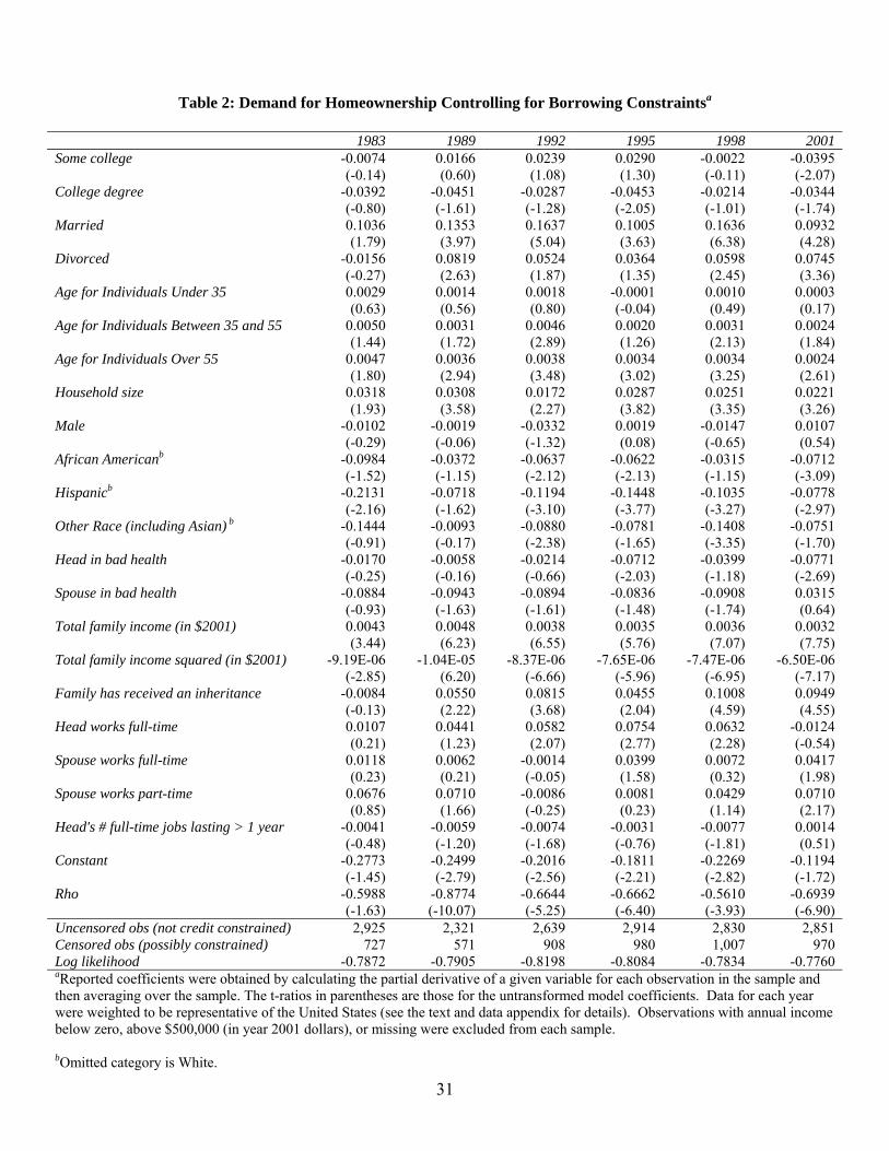
described earlier.15 Results from this exercise provide estimates of the demand for

homeownership when households are subject only to their budget constraint. These estimates are

presented in Table 2. Second, we estimate homeownership over all households as described

earlier. Results from this exercise provide estimates of the observed or actual likelihood of

homeownership in the presence of both household budget and credit constraints. These estimates

are presented in Table 3. Differencing estimates from these two exercises enables us to isolate

the effects of credit constraints on homeownership attainment. These measures are presented in

Table 4.

In reviewing these tables several points regarding sample composition and the format in

which the estimates are presented should be emphasized. First, all of our estimates are based on

samples that exclude individuals reporting household income that is negative or above $500,000

(in 2001 dollars).16 Also, results are provided separately for the survey years 1983, 1989, 1992,

1995, 1998, and 2001. Third, Tables 2 through 4 present partial derivatives for the probit model

coefficients. Those partial derivatives are calculated for each observation in the sample and the

sample means as derive there from are then reported. As such, the reported coefficients indicate

the percentage point influence of a given household attribute on homeownership attainment. The

15As described earlier, the full sample reported in Table 2 is used to estimate the selection equation while the censored observations are omitted when estimating the homeownership equation. Estimates from the selection equation that determines who is not credit constrained are not reported to conserve space. 16Especially at the upper end, the SCF includes a small number of extremely high-income households and these individuals are removed from their sample to ensure that they do not unduly influence the results.

12

numbers in parentheses below the coefficients are t-ratios from the original probit model

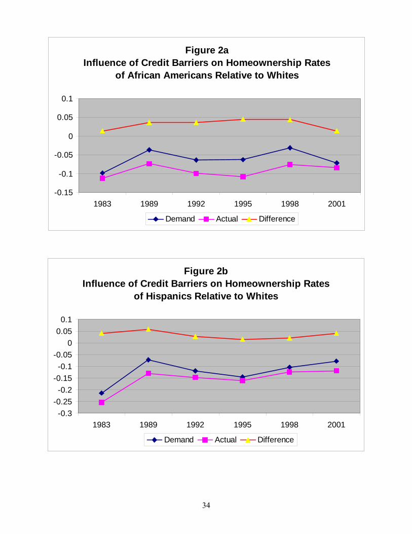
coefficients. Finally, to facilitate review of the race-related effects, Figures 2a and 2b plot select

findings from these tables. Specifically, results for African-Americans from each of the three

tables are plotted in Figure 2a. Results for Hispanics are plotted in Figure 2b.

Consider the influence of race and ethnicity. Several patterns stand out in Figures 2a and

2b. Relative to white households, in 1983, demand for homeownership among African

Americans and Hispanics was roughly 10 and 20 percentage points lower, respectively. Those

very large disparities in demand narrowed markedly in the following decade and were roughly

7.1 and 7.8 percentage points for African Americans and Hispanics in 2001, respectively. It is

noteworthy that this narrowing of racial differences in demand for homeownership was broadly

consistent with changes in the home savings behavior of white and minority households over the

survey period, especially changes that occurred in the 1980s: race-related differences in savings

behavior were substantial in 1983 but had narrowed considerably by 1989.17

Also apparent in Figure 2a, in the early 1980s, the observed or actual propensity for

homeownership among blacks was roughly 11 percentage points lower than among comparable

white households in the early 1980s. That differential narrowed sharply over subsequent years to

about 8 percentage points in the latter part of the 1990s. An analogous pattern was evidenced for

Hispanics with the white-Hispanic difference in the actual propensity for homeownership in

Figure 2b narrowing from 25 percentage points in 1983 to just under 12 percentage points in

2001.

The patterns just discussed reveal an important race-related effect in demand for and

actual homeownership propensities even after controlling for a host of household demographic

17Bear in mind of course that the estimates in Figures 2a and 2b reflect the influence of race after controlling for a host of other households attributes, while the patterns in Figure 1 are summary measures across race without controlling for other household attributes.

13

and financial attributes. To what extent do credit barriers account for these estimated racial

differentials? Estimates in Table 4 and in Figures 2a and 2b suggest that credit barriers explain

relatively little of the estimated homeownership race effects. In this regard, several points are

worth emphasizing. First, much of the increase in demand for homeownership among black and

Hispanic households over the 1983 to 2001 period was realized in actual homeownership gains.

For that reason, relative to white households, the estimated influence of credit barriers on minority

homeownership rates has remained relatively stable throughout the 1990s. Further, in all years

from 1983 to 2001, credit barriers account for less than 5 percentage points of the white-minority

gap in homeownership rates for both African American and Hispanic households, or about one-

fifth of the overall racial gap in homeownership rates. From a policy perspective, this implies that

further innovation in mortgage finance is unlikely to substantially affect racial disparities in access

to homeownership. Moreover, and arguably more provocative, as abhorrent has discrimination

may be, the evidence suggests that mortgage market discrimination has been of only limited

importance in the explanation of racial gaps in homeownership.

Finally, in addition to race, it is evident in Tables 2, 3, and 4 that a number of other

household economic and demographic factors also affect homeownership and the influence of

credit barriers. Consistent with results in the homeownership choice literature, those factors

include, for example, age, marital status, and employment status. However, because access to

homeownership among minority households has been at the center of recent and sometimes

heated policy debates, we have chosen to pay special attention to those effects here.

14

IV. Decomposition of Changes in Aggregate Homeownership Rates

4.1 Decomposition: Methods

The estimates in Tables 2 through 4 can be used to decompose changes in homeownership

rates across years into effects resulting from changes in economic and demographic characteristics

of the population versus changes in market conditions. As an illustration, consider the years 1989

and 1998. To further simplify the discussion, define X1989 and X1998 to be the average

characteristics of the samples from 1989 and 1998, respectively, b1989 and b1998 are the estimated

demand coefficients from equation (2.2), and I1989 and I1998 are the overall sample owner-

occupancy rates from the respective years.

Our goal is to explain I1998 – I1989, the change in homeownership rate over the 1989 to 1998

period. Accordingly, we write I1998 and I1989 as

I1998 = X1998b1998 – C1998 (3.1a) and I1989 = X1989b1989 – C1989 (3.1b) where X1998b1998 and X1989b1989 are the percentage of the population that would own in the absence

of credit barriers – the demand or preference for homeownership – and C1998 and C1998 are the

influence of credit barriers on homeownership rates, positive values for which imply that credit

barriers reduce homeownership.

Differencing equations (3.1a) and (3.1b) over the two time periods yields

I1998 – I1989 = [X1998b1998 – X1989b1989] – [C1998 – C1989] (3.2)

where the first bracketed term is the change in the demand for homeownership while the second

bracketed term reflects the change in the influence of credit barriers on homeownership.

What fraction of the change in the demand for homeownership – the preferred

homeownership rate – can be attributed to changes in household demographic/financial attributes

15

as opposed to factors that affect the coefficients in the model? To address that question, the first

term in (3.2) is further decomposed as follows:

I1998 – I1989 = X1998[b1998 – b1989] + [X1998 – X1989]b1989 – [C1998 – C1989]. (3.3)

Observe that the first two bracketed terms in (3.3) reflect the demand for homeownership in the

absence of binding credit barriers. The third bracketed term measures the level of unfulfilled

demand arising from the influence of credit barriers. We will examine the role of each of these

terms in turn.

In equation (3.3), the first bracketed term, X1998[b1998 – b1989], captures changes in the

demand for homeownership arising from changes in cultural norms and the cost of owning. If

cultural norms and the cost of owning do not change, then the estimated coefficient vector would

not change and the first bracketed term would drop out of the model. In considering that

possibility, it is important to remember that b1998 and b1989 each includes a constant term as well as

a vector of coefficients for the household attributes. The constant terms reflect macroeconomic

conditions common to households in a given year. In that regard, b1998 – b1989 captures not only

changes in the influence of a given set of demographic traits, but also the effect of changes in

mortgage interest rates and innovations in the mortgage market that affect demand for

homeownership.

The second bracketed term, [X1998 – X1989]b1989, captures changes in the demand for

homeownership arising only from changes in the attributes of the population, such as the

distribution of income, race, and marital status. In addition, increases in household income as

occurred during the economic boom of the 1990s would be captured here.

Consider now the third bracketed term in equation (3.3a), [C1998 – C1989]. Credit barriers

restrict access to homeownership when the level of debt lenders are willing to provide is less than

16

the amount requested by households. Accordingly, it is desirable to further decompose the

influence of credit barriers in (3.3) into changes arising from the characteristics of the population

that affect the demand for mortgage debt versus changes arising because of a shift in the propensity

of a given type of household to encounter binding credit barriers. This can be accomplished as

indicated below.

As displayed in Table 3, we estimate a second homeownership model over all households

(including credit constrained families) without controls for the influence of credit barriers. This

later model yields an alternative set of coefficients, at, where

I1998 = X1998a1998 , (3.4)

and I1998 is the 1998 homeownership rate as before. Now define c1998 ≡ b1998 – a1998, where b1998

are the coefficients from equation (3.1a) and a1998 are the coefficients from (3.4). Then from

equations (3.1a) and (3.4), X1998c1998 = C1998 where c1998 is the marginal effect of X1998 on credit

barriers. Hence, the third bracketed term in (3.3) can be written as

C1998 – C1989 = c1998X1998 - c1989X1989 .

Decomposing as in equation (3.2),

C1998 – C1989 = [X1998 – X1989]c1989 + X1998[c1998 - c1989] . (3.5)

The first bracketed term in equation (3.5) makes explicit that changes in the

characteristics of the population affect the degree to which credit barriers influence

homeownership rates holding constant macroeconomic and mortgage market conditions in the

initial year. The second bracketed term in equation (3.5) makes explicit that changes in interest

rates and mortgage market conditions – as reflected in the constant terms in c1998 and c1989 – as

well as changes in the influence of individual household attributes (e.g. white, black, married)

also affect the degree to which credit barriers influence homeownership rates.

17

Substituting equation (3.5) into (3.3) we obtain an expression for the change in

homeownership rates decomposed into four bracketed terms.

I1998 - I1989 = X1998[b1998 – b1989 ] + [X1998 – X1989]b1989

– [X1998 – X1989]c1989 – X1998[c1998 - c1989] . (3.6)

Recognizing that the first three bracketed terms above capture demand side effects, the last

bracketed term in (3.6) is of particular interest. In particular, a decrease in the influence of the

last bracketed term would imply that, holding constant the demand for homeownership, the

influence of credit barriers on homeownership rates has diminished. That in turn, would be

consistent with a relaxation of credit barriers.18

4.2 Decomposition Results

Table 5 presents results of the decomposition exercise for all SCF survey years from

1983 to 2001. The table is divided into three panels. The top panel utilizes coefficients from

Table 3 to estimate “actual” homeownership rates without controlling for the influence of credit

constraints. The middle panel utilizes coefficients from Table 2 to estimate “demand” for

homeownership in a manner that controls for the influence of credit constraints as described

earlier. The bottom panel differences estimates from the first two panels and in so doing

identifies the influence of credit barriers.

Observe also that each of the three panels provides a six-by-six matrix of estimates. Each

row is based on coefficients from a given survey year as drawn from one of the columns in

Tables 2, 3, or 4 depending on the panel in question. For example, the top row in each panel is

18A reduced influence of the last bracketed term could also arise if households seek smaller loans holding constant lender imposed credit standards. However, in the context of the 1990s in which dramatic innovations in low-income and low-downpayment mortgage lending occurred, it seems more likely that a reduction in the last bracketed term would derive from those innovations.

18

based on 1983 coefficients and the bottom row is based on 2001 coefficients, with the

intervening years in sequential order. Looking across the columns, coefficients from a given

year are applied to data for each of the different sample years. For example, the left-hand

column of each panel combines coefficients from each sample year with the 1983 sample data.

Likewise, the right-hand column of each panel combines coefficients from each sample year with

the 2001 sample data. It follows that the main diagonal elements of a given panel correspond to

coefficients and sample drawn from the same survey year and as such, provide estimates of

patterns that truly prevailed in that year. Off-diagonal elements provide estimates of patterns

that would have prevailed in a given year had the coefficients or sample differed in the manner

specified.

Consider now the top panel of Table 5 and recall that this panel reports estimates of

“actual” homeownership rates. In the lower right corner, the estimated homeownership rate in

2001 is 67.2 percent. In contrast, in the upper left corner the estimated homeownership rate in

1983 is 62.6 percent, 4.6 percentage points lower. To what extent does the increase in

homeownership over this period reflect changes in household behavior as opposed to changes in

the demographic and financial attributes of the population from each of the survey years? To

answer that question, consider the following.

Applying 1983 coefficients to the 2001 sample (top row, far right column), the estimated

homeownership rate equals 64.5 percent. That value is roughly 2 percentage points higher than

the actual homeownership rate in 1983, and roughly 3 percentage points lower than the actual

homeownership rate in 2001. Thus, changes in the composition of the population between 1983

and 2001 contributed 2 percentage points to the increase in homeownership rates over that

period. Changes in household behavior account for the remaining 3 percentage points. The

19

former effect includes changes in the distribution of household real income associated with the

boom of the 1990s, as well as changes in other household attributes captured in the

homeownership model in Table 3. The latter effect includes the influence of changes in market

conditions such as interest rates, mortgage financing innovations, and changes in norms and

preferences for homeownership, all of which can cause the estimated coefficients of one sample

year to differ from those of another sample year.

Focus next on the middle panel of Table 5 and recall that this panel decomposes changes

in the demand for homeownership. For 1983 the estimated demand for homeownership was 71.2

percent (upper left corner of the panel). In 2001 the estimated demand for homeownership was

78.4 percent (bottom right corner of the panel). Overall, demand for homeownership appears to

have increased by about 7.2 percentage points over the 1983 to 2001 period. But, applying the

1983 coefficients to the 2001 data, the predicted demand for homeownership is 71.5 percent.

That value is only 0.3 percentage point higher than the estimated rate in 1983 and 6.9 percentage

points lower than the estimated rate in 2001. On balance, these patterns imply that changes in

household behavior – not changes in the composition of the population – account for nearly the

entire increase in demand for homeownership over the 1983 to 2001 period.

The patterns just described are mirrored in the bottom panel of Table 5. That table

examines the influence of credit barriers on homeownership rates. In 1983 and 2001 credit

barriers are estimated to have depressed homeownership rates by 8.6 and 11.1 percentage points,

respectively. Decomposing this change as above, it is clear that the increase in the influence of

credit barriers over this period is being driven predominantly by changes in the model

coefficients as opposed to changes in the attributes of the population.

20

Summarizing the discussion above, demand for homeownership rose by over 7

percentage points from 1983 to 2001. However, only 4.6 percentage points of that increase in

demand was realized. The remainder is reflected in an increase in the influence of credit barriers

as can be seen in the bottom panel of Table 5.

The discussion thus far has focused just on the beginning and end of our sample horizon,

1983 and 2001. Although informative, that comparison does not do justice to the changes in the

intervening years. Accordingly, Figure 3a plots the last row from each of the three panels in

Table 5. Recall that this row is based on year 2001 coefficients and that these coefficients are

then applied to the samples from each of the different survey years. Also, it should be

emphasized that the patterns in Figure 3a are very similar to those for the other survey year rows

in Table 5.

In Figure 3a, observe that the “actual” homeownership rate is predicted to fall from 63.8

percent in 1983 to 61.6 percent in 1989, but then is predicted to rise continuously to its peak of

67.2 in 2001. This implies that an increase in actual homeownership rates of 5.6 percentage

points over the decade of the 1990s can be attributed to changes in the financial and demographic

attributes of the population. A similar but more muted pattern is evident for the demand for

homeownership. Demand is initially forecast to be 77.3 percent in 1983, falls to 75.0 in 1989,

and then rises monotonically to 78.4 in 2001. This implies an increase in demand for

homeownership of 3.4 percentage points over the decade of the 1990s that can be attributed to

changes in the attributes of the population. Together, these patterns imply that changes in the

attributes of the population had little impact on the influence of credit barriers in the 1980s, but

contributed to a 2.3 percentage point decline in the influence of credit barriers from 1989 to

2001. More generally, from Figure 3a it is clear that shifts in the financial and demographic

21

attributes of the population in the 1990s boosted demand for homeownership and reduced the

influence of credit barriers.

Figure 3b considers the influence of changes in the intrinsic behavior of individuals, as

reflected in the model coefficients. Specifically, the figure plots the last column from each of the

three panels in Table 5.19 Recall that this column is based on the year 2001 sample and that this

sample is then applied to the coefficients from each of the different survey years. This figure

displays a different pattern. Changes in the behavior of individuals imply a sharp increase in

demand for homeownership from 1983 to 1989, only a portion of which was realized in an

“actual” increase in homeownership. That disparity leads to a sharp uptick in the influence of

credit barriers on homeownership rates, from 7 percentage points in 1983 to 10 percentage points

in 1989.

Following 1989, estimates of the “actual” homeownership rate decline slightly

throughout the 1990s, as does the demand for homeownership. The primary exception is a

market increase in demand from 1998 to 2001, with an accompanying increase in the influence

of credit barriers.

Comparing the patterns in Figure 3b with those in Figure 3a, it is clear that during the

decade of the 1990s two important factors influenced homeownership. On the one hand, changes

in the financial and demographic attributes of the population served to boost demand for

homeownership and to reduce the influence of credit barriers throughout the decade. Changes in

the behavior of individual households however – as reflected in the model coefficients – reduced

19We choose the column corresponding to the year 2001 coefficients to facilitate comparison to the patterns just noted. Note, however, that the patterns revealed in Figure 3b are nearly identical for the other survey year columns in Table 5 but are not presented to conserve space.

22

both demand and the influence of credit barriers until 1998 and then subsequently pushed both

higher.

4.3 Robustness Checks

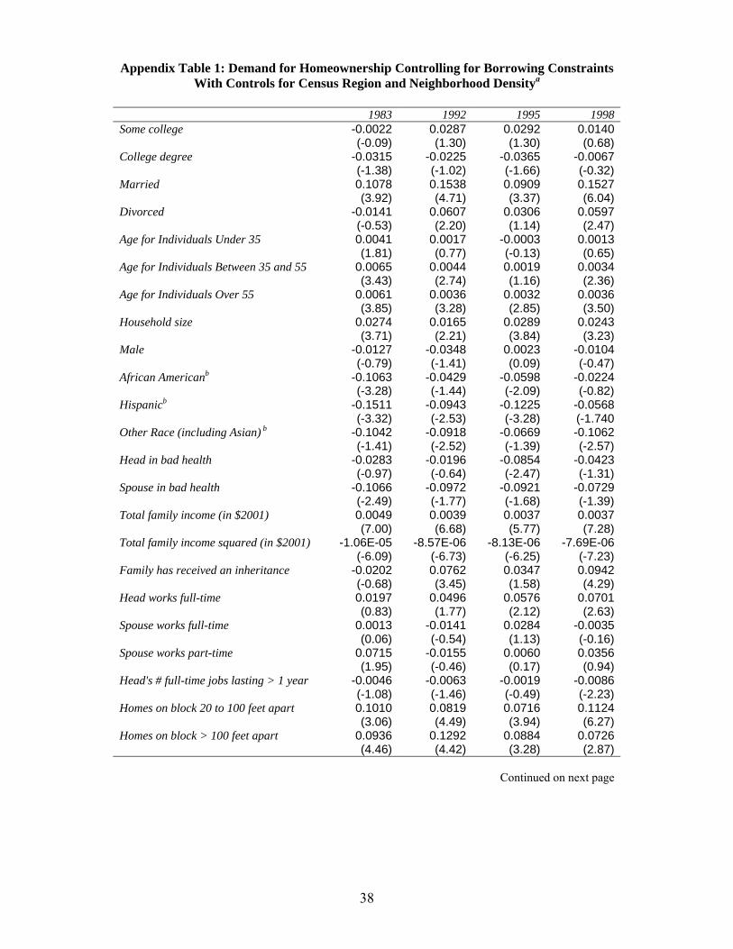
As a robustness check, we repeated the entire exercise above using a richer set of control

variables in the underlying probit models that are available in just four of the sample years, 1983,

1992, 1995, and 1998. These additional variables include controls for the four census regions in

the United States and also for the density of development in the local neighborhood.

Decomposition results based on this specification appear in Table 6, while the underlying Probit

model coefficients are reported in the Appendix.

Two points become apparent when comparing findings in Table 6 to those in Table 5.

First, the qualitative pattern of the changes in the influence of credit barriers over time is similar

in Table 6 as compared to Table 5. Specifically, observe that the influence of credit barriers in

Table 6 peaks in 1992 (at 11.1 percentage points), and then declines continuously to 8.9

percentage points in 1998, the same qualitative pattern as in Table 5.

Second, the magnitude of the influence of credit barriers is reduced when additional

control variables are added to the model. For example, in 1998, the estimated influence of credit

barriers in Table 6 (lower right corner) is 8.9 percentage points versus 9.6 percentage points in

Table 5.

Because of idiosyncratic differences in the data files for different years, the set of

variables available for 1998 is more complete than for any other survey year. For that reason, we

further augment the 1998 regression by including controls for several additional variables.

Specifically, we begin by retaining all variables included in the model reported in the appendix

23

and used to produce Table 6. In addition, both the housing tenure and credit constraint models

were further augmented by including controls for (i) whether household total income rose faster

than the rate of inflation in the last five years, (ii) whether total household income is expected to

rise faster than inflation in the coming year, and (iii) whether the household expects to receive an

inheritance or future transfer of assets at some point in the future. The credit model was further

expanded by including a measure of whether the household head or spouse had filed for

bankruptcy in the past five years. Results from this specification indicate that credit barriers

reduced homeownership rates in 1998 by 6.5 percentage points, a further decline relative to

Tables 5 and 6.20

Summarizing, the qualitative patterns with regard to changes in the influence of credit

barriers appear largely robust to inclusion of additional covariates in the models, at least to the

extent that the data allow us to investigate this issue. However, it is apparent that including

additional control variables tends to work in the direction of reducing the estimated influence of

credit barriers. With that in mind, we feel it is prudent to view the estimated impacts of credit

barriers in Tables 5 and 6 as upper bounds.

V. Conclusions

U.S. homeownership rates rose by roughly 3-1/2 percentage points during the 1990s to

67.2 percent in 2001, a historically high level. The upward movement in homeownership

coincided with shifts in the composition of the population, innovations in mortgage finance, the

20In Rosenthal (2002), the estimated influence of credit barriers in 1998 was lower still, 4.05 percentage points. However, in that paper, farm households were omitted while all other families were retained (including those with income above $500,000). In addition, the set of covariates in the prior paper did not include the regional controls but included some additional measures pertaining to education and the value of past and anticipated future inheritances and settlements. These differences account for the difference in estimates between the two papers and further underscore that the magnitude of the estimated influence of credit barriers is somewhat sensitive to model specification.

24

economic boom of the 1990s, and declining interest rates. Using six waves of the Federal

Reserve Board’s Survey of Consumer Finances, this paper analyzes the determinants of changes

in homeownership rates in the 1980s and 1990s, with particular attention to racial gaps in

homeownership. The analysis is unique to the literature in applying the same model

specification to different years of the Survey of Consumer Finances: 1983, 1985, 1989, 1992,

1995, 1998, and 2001. This ensures that changes in the estimated patterns over time are not

driven by changes in the quality of the data or in model specification.

Results indicate that changes in population demographic and financial attributes account

for most of the increase in demand for homeownership (and actual homeownership rates)

between 1989 and 2001. This implies that innovations in mortgage finance and declining

interest rates, while clearly important for a host of reasons, likely were not the primary drivers of

the rise in homeownership during the 1990s.

New to the literature, we also demonstrate that minority renters were substantially less

likely to save for homeownership in the early 1980s relative to white households. However,

those differences in savings behavior have narrowed continuously over the past two decades and

disappeared in 2001. Nevertheless, white-minority gaps in homeownership rates remained at or

above 25 percentage points throughout the 1980s and 1990s. Further, by the end of the 1990s,

demographic and financial attributes were estimated to account for all but 8 percentage points of

the racial disparities in homeownership. Of that residual, credit barriers account for no more

than 5 percentage points. Policy makers, therefore, will have to look beyond mortgage market

innovation if their goal is to substantially reduce racial disparities in homeownership.

Finally, we also examine the overall influence of credit barriers on U.S. homeownership

rates as well as the sensitivity of our results to the inclusion of additional control variables for

25

those survey years in which a richer set of covariates is available. Results suggest that the

qualitative patterns regarding changes over time in the influence of credit barriers are robust.

However, it is also clear that the estimated influence of credit barriers on aggregate U.S.

homeownership rates tends to decline with a more complete model specification. Our most

reliable estimate of the influence of credit barriers on homeownership rates is based on an

expanded model specification for 1998. Results from that model suggest that credit barriers

depressed homeownership rates in 1998 by roughly 6.6 percentage points, but that estimate

should be viewed as an upper bound for reasons just noted.

26

REFERENCES Bank of America. 1998. Bank of America Launches First Ever Widely Available Zero Down Payment Mortgage. Bank of America news release, March 2. Boehm, Thomas H. Herzog, and A. Schlottmann, “Intra-Urban Mobility, Migration, and Tenure Choice,” The Review of Economics and Statistics, 73(1), 59-68, 1991. Boyes, W., D. Hoffman, and S. Low. 1989. An Econometric Analysis of the Bank Credit Scoring Problem. Journal of Econometrics 40(1): 3-14. Canner, G., and D. Smith. 1991. Home Mortgage Disclosure Act: Expanded Data on Residential Lending. Federal Reserve Bulletin (November): 859-81. Coulson, Edward, “Why are Hispanic- and Asian-American Homeownership Rates So Low?: Immigration and Other Factors,” Journal of Urban Economics, 45, 209-227, 1999. Edin, P-A. and Peter Englund, “Moving Costs and Housing Demand: Are Recent movers really in Equilibrium?” Journal of Public Economics, 44, 299-320, 1991. Gabriel, Stuart and Gary Painter, “Paths to Homeownership: An Analysis of the Residential Location and Homeownership Choices of Black Households” Working Paper No. 01-03, Research Institute for Housing America Working Paper, October 2001. Journal of Real Estate Finance and Economics, Volume 27, Issue 1, 2003. Gabriel, Stuart and Stuart Rosenthal. “Household Location and Race: Estimates of a Multinomial Logit Model,” Review of Economics and Statistics, 71: 218-234, 1989. Gyourko, Joseph and Peter Linneman, “An analysis of the changing influences on traditional household ownership patterns,” Journal of Urban Economics, 39, 318-341, 1996. Ihlanfeldt, Keith, “An empirical investigation of alternative approaches to estimation of the equilibrium demand for housing,” Journal of Urban Economics, 9, 97-105, 1981. Kennickell, Arthur, “Revisions to the SCF Weighting Methodology: Accounting for Race/Ethnicity and Homeownership,” Federal Reserve Board working paper, January 1999. Kennickell, Arthur, “Multiple Imputation in the Survey of Consumer Finances,” Federal Reserve Board working paper, September 1998. Maddala, G. 1983. Limited-Dependent and Qualitative Variables in Econometrics. New York: Cambridge University Press. Munnell et al (1996), “Mortgage Lending in Boston: Interpreting the HMDA Data”, American Economic Review 86 (March) 25-53. Painter, Gary, Stuart Gabriel, and Dowell Myers, “The Decision to Own: The Impact of Race, Ethnicity, and Immigrant Status,” RIHA working paper No. 00-02, 2000, Journal of Urban Economics, 49, 150-167, 2001.

27

Rehm, B. 1991a. ABA Rebuts Bias Charge in Fed Study on Lending. American Banker, October 15, 1 and 19. Rehm, B. 1991b. Data on Bias in Lending Sparks Demands for Action. American Banker, October 22, 1 and 9. Rosenthal, Stuart, “Eliminating Credit Barriers to Increase Homeownership: How Far Can We Go?”, Research Institute for Housing America working paper 01-01, 2001, in Low-Income Homeownership: Examining the Unexamined Goal, eds. Eric Belsky and Nicolas Retsina, Brookings Institution Press, Washington D.C., 2002. Rosenthal, Stuart S., “A Residence Time Model of Housing Markets,” Journal of Public Economics, 36: 87-109, 1988. Turner, Margery Austin, Fred Freiberg, Erin Godfrey, Carla Herbig, Diane K. Levy, and Robin R. Smith, “All Other Things Being Equal: A Paired Testing Study of Mortgage Lending Institutions,” U.S. Department of Housing and Urban Development, Office of Fair Housing and Equal Opportunity,” http://www.huduser.org/Publications/PDF/aotbe.pdf , April 2002(a). Turner, Margery Austin, Stephen L. Ross, George C. Galster, and John Ying, with Erin B. Godfrey, Beata A. Bednarz, Carla Herbig, Seon Joo Lee, AKM. Rezaul Hossain, and Bo Zhao, “Discrimination in Metropolitan Housing Markets: National Results from Phase I HDS 2000” U.S. Department of Housing and Urban Development” http://www.huduser.org/Publications/pdf/Phase1_Report.pdf, November 2002(b). Tunali, I. 1986. A General Structure for Models of Double-Selection and an Application to a Joint Migration/Earnings Process with Remigration. Research in Labor Economics 8(B): 235-282. Wachter, Susan and Isaac Megbolugbe, “Racial and Ethnic Disparities in Homeownership,” Housing Policy Debate, 3, 333-370, 1992.

28

Appendix: Data

Data for the analysis are taken from the Survey of Consumer Finances (SCF) for the years

1983, 1989, 1992, 1995, 1998, and 2001. These surveys are independent cross-sections with the

exception of the 1983 and 1989 surveys for which a portion of the 1983 families appear again in

1989. The SCF is uniquely suited for addressing the research questions because it provides

substantial detail on individual household financial and demographic characteristics, along with a

number of unique questions on expectations of future behavior and access to credit.

Each year of the SCF provides data on roughly 4,500 households. Sampling weights

provided with the data permit one to weight the data such that results are representative of the

United States population.21 In addition, beginning in 1989, a sophisticated procedure is used to

impute missing values. In part, this includes the creation of five “implicates” of the data, where

each is an alternate version of the entire dataset but with slightly different imputations. Kennickell

(1998) provides details on how to interpret and work with the implicates. 22

The Survey of Consumer Finances (SCF) provides unusually rich information on the

financial characteristics of households. Of the SCF sample of about 4500 households, roughly

2,800 are selected so as to be representative of the entire United States while the remaining

households over-represent wealthy families and are drawn from tax files. To protect

confidentiality, the public use version of the 1998 SCF does not allow the analyst to separately

identify the representative and tax-based samples. However, sampling weights provided with the

21Kennickell (1999) provides a careful discussion of the SCF sampling weights and shows that the sample moments of the weighted SCF data match the Consumer Population Survey (CPS). See also Rosenthal (2002) for further discussion of the SCF. 22The SCF data are imputed five times to control for missing values and also to protect the confidentiality of some respondents with especially unusual and highly visible characteristics (such as very high wealth). When estimating the bivariate probit models, all five implicates totaling over 21,000 records were used and the standard errors were divided by the square root of 5 to adjust for the “true” sample size. See the 1998 SCF manual and Kennickell (1998) for details.

29

data permit one to weight the data such that results are representative of the entire United States.

The bivariate probit model was estimated using unweighted data to obtain the parameter estimates

on the assumption that all the covariates in the model are exogenous. The simulations, in contrast,

were calculated using the sampling weights to ensure that the simulation results are representative

of the United States.23

A final point concerns sample composition. All of the analysis in this paper is conducted

using non-farm households with household heads between ages 18 through 65 and annual income

between $10,000 and $200,000 in 2001 dollars. These restrictions were imposed in order to focus

on the set of households most subject to policy attention with respect to opportunities for

homeownership.

23See Kennickell (1999) for a careful discussion of the SCF sampling weights.

30

Table 1: Homeownership Rates and the Percent of Households Saving to Buy a Home

Sample Composition: Household Heads Aged 18 Through 65a

1983 1989 1992 1995 1998

2001

Homeownership Rate

All Households 0.628 0.638 0.639 0.645 0.660 0.673 White Households 0.673 0.704 0.703 0.704 0.716 0.737 Black Households 0.440 0.424 0.436 0.427 0.461 0.475

Hispanic Households 0.314 0.419 0.399 0.429 0.441 0.442

Saving to Buy a Home All Households 0.058 0.063 0.057 0.071 0.070 0.069

All Owners

0.026 0.018 0.017 0.026 0.022 0.017

All Renters 0.111 0.141 0.127 0.152 0.162 0.176 White Renters 0.124 0.169 0.118 0.167 0.150 0.171 Black Renters 0.068 0.063 0.125 0.134 0.165 0.157

Hispanic Renters

0.085 0.113 0.189 0.110 0.248 0.224

aAll estimates are based on data from different years of the Survey of Consumer Finances and are weighted to be representative of the United States. Excludes families with total family income (in $2001) below zero, above $500,000, or missing.

Figure 1: Saving to Buy a Home

0

0.05

0.1

0.15

0.2

0.25

0.3

1983 1989 1992 1995 1998 2001Year

Perc

enta

ge S

avin

g to

Buy

a H

ome

All Owners White RentersBlack Renters Hispanic Renters

31

Table 2: Demand for Homeownership Controlling for Borrowing Constraintsa

1983 1989 1992 1995 1998 2001 Some college -0.0074 0.0166 0.0239 0.0290 -0.0022 -0.0395 (-0.14) (0.60) (1.08) (1.30) (-0.11) (-2.07) College degree -0.0392 -0.0451 -0.0287 -0.0453 -0.0214 -0.0344 (-0.80) (-1.61) (-1.28) (-2.05) (-1.01) (-1.74) Married 0.1036 0.1353 0.1637 0.1005 0.1636 0.0932 (1.79) (3.97) (5.04) (3.63) (6.38) (4.28) Divorced -0.0156 0.0819 0.0524 0.0364 0.0598 0.0745 (-0.27) (2.63) (1.87) (1.35) (2.45) (3.36) Age for Individuals Under 35 0.0029 0.0014 0.0018 -0.0001 0.0010 0.0003 (0.63) (0.56) (0.80) (-0.04) (0.49) (0.17) Age for Individuals Between 35 and 55 0.0050 0.0031 0.0046 0.0020 0.0031 0.0024 (1.44) (1.72) (2.89) (1.26) (2.13) (1.84) Age for Individuals Over 55 0.0047 0.0036 0.0038 0.0034 0.0034 0.0024 (1.80) (2.94) (3.48) (3.02) (3.25) (2.61) Household size 0.0318 0.0308 0.0172 0.0287 0.0251 0.0221 (1.93) (3.58) (2.27) (3.82) (3.35) (3.26) Male -0.0102 -0.0019 -0.0332 0.0019 -0.0147 0.0107 (-0.29) (-0.06) (-1.32) (0.08) (-0.65) (0.54) African Americanb -0.0984 -0.0372 -0.0637 -0.0622 -0.0315 -0.0712 (-1.52) (-1.15) (-2.12) (-2.13) (-1.15) (-3.09) Hispanicb -0.2131 -0.0718 -0.1194 -0.1448 -0.1035 -0.0778 (-2.16) (-1.62) (-3.10) (-3.77) (-3.27) (-2.97) Other Race (including Asian) b -0.1444 -0.0093 -0.0880 -0.0781 -0.1408 -0.0751 (-0.91) (-0.17) (-2.38) (-1.65) (-3.35) (-1.70) Head in bad health -0.0170 -0.0058 -0.0214 -0.0712 -0.0399 -0.0771 (-0.25) (-0.16) (-0.66) (-2.03) (-1.18) (-2.69) Spouse in bad health -0.0884 -0.0943 -0.0894 -0.0836 -0.0908 0.0315 (-0.93) (-1.63) (-1.61) (-1.48) (-1.74) (0.64) Total family income (in $2001) 0.0043 0.0048 0.0038 0.0035 0.0036 0.0032 (3.44) (6.23) (6.55) (5.76) (7.07) (7.75) Total family income squared (in $2001) -9.19E-06 -1.04E-05 -8.37E-06 -7.65E-06 -7.47E-06 -6.50E-06 (-2.85) (6.20) (-6.66) (-5.96) (-6.95) (-7.17) Family has received an inheritance -0.0084 0.0550 0.0815 0.0455 0.1008 0.0949 (-0.13) (2.22) (3.68) (2.04) (4.59) (4.55) Head works full-time 0.0107 0.0441 0.0582 0.0754 0.0632 -0.0124 (0.21) (1.23) (2.07) (2.77) (2.28) (-0.54) Spouse works full-time 0.0118 0.0062 -0.0014 0.0399 0.0072 0.0417 (0.23) (0.21) (-0.05) (1.58) (0.32) (1.98) Spouse works part-time 0.0676 0.0710 -0.0086 0.0081 0.0429 0.0710 (0.85) (1.66) (-0.25) (0.23) (1.14) (2.17) Head's # full-time jobs lasting > 1 year -0.0041 -0.0059 -0.0074 -0.0031 -0.0077 0.0014 (-0.48) (-1.20) (-1.68) (-0.76) (-1.81) (0.51) Constant -0.2773 -0.2499 -0.2016 -0.1811 -0.2269 -0.1194 (-1.45) (-2.79) (-2.56) (-2.21) (-2.82) (-1.72) Rho -0.5988 -0.8774 -0.6644 -0.6662 -0.5610 -0.6939 (-1.63) (-10.07) (-5.25) (-6.40) (-3.93) (-6.90) Uncensored obs (not credit constrained) 2,925 2,321 2,639 2,914 2,830 2,851 Censored obs (possibly constrained) 727 571 908 980 1,007 970 Log likelihood -0.7872 -0.7905 -0.8198 -0.8084 -0.7834 -0.7760 aReported coefficients were obtained by calculating the partial derivative of a given variable for each observation in the sample and then averaging over the sample. The t-ratios in parentheses are those for the untransformed model coefficients. Data for each year were weighted to be representative of the United States (see the text and data appendix for details). Observations with annual income below zero, above $500,000 (in year 2001 dollars), or missing were excluded from each sample. bOmitted category is White.

32

Table 3: Actual Propensity for Homeownership Without Controlling for Borrowing Constraintsa

1983 1989 1992 1995 1998 2001 Some college -0.0240 0.0243 0.0284 0.0028 0.0014 -0.0460 (-0.54) (0.98) (1.40) (0.14) (0.08) (-2.61) College degree -0.0403 -0.0220 -0.0191 -0.0330 -0.0279 -0.0258 (-0.88) (-0.85) (-0.91) (-1.60) (-1.42) (-1.33) Married 0.1181 0.1767 0.1962 0.1432 0.1770 0.0984 (2.40) (5.71) (7.47) (6.24) (8.33) (4.86) Divorced -0.0042 0.1033 0.0201 0.0392 0.0504 0.0631 (-0.08) (3.62) (0.80) (1.59) (2.28) (2.98) Age for Individuals Under 35 0.0092 0.0056 0.0064 0.0031 0.0038 0.0073 (2.23) (2.40) (3.04) (1.48) (2.04) (3.94) Age for Individuals Between 35 and 55 0.0102 0.0071 0.0088 0.0057 0.0060 0.0083 (3.60) (4.41) (5.96) (3.97) (4.79) (6.65) Age for Individuals Over 55 0.0092 0.0079 0.0080 0.0068 0.0064 0.0077 (4.85) (7.33) (8.16) (6.92) (7.50) (8.81) Household size 0.0300 0.0322 0.0089 0.0244 0.0193 0.0228 (2.14) (4.70) (1.31) (3.79) (3.06) (3.85) Male -0.0019 0.0110 -0.0468 -0.0346 -0.0109 0.0074 (-0.06) (0.41) (-2.04) (-1.55) (-0.52) (0.38) African Americanb -0.1122 -0.0739 -0.0999 -0.1075 -0.0751 -0.0844 (-2.35) (-2.78) (-4.19) (-4.81) (-3.37) (-4.14) Hispanicb -0.2536 -0.1298 -0.1470 -0.1597 -0.1239 -0.1187 (-2.89) (-3.67) (-4.80) (-4.78) (-4.48) (-4.74) Other Race (including Asian) b -0.0914 -0.0440 -0.0831 -0.1362 -0.1401 -0.1129 (-0.65) (-1.01) (-2.32) (-3.37) (-3.57) (-2.68) Head in bad health 0.0228 -0.0379 -0.0038 -0.0667 -0.0760 -0.0652 (0.35) (-1.09) (-0.12) (-1.99) (-2.25) (-2.24) Spouse in bad health -0.1042 -0.0559 -0.0758 -0.0519 -0.0953 -0.0078 (-1.17) (-0.96) (-1.40) (-0.97) (-2.09) (-0.17) Total family income (in $2001) 0.0052 0.0052 0.0044 0.0045 0.0047 0.0045 (4.73) (7.61) (8.81) (8.09) (10.71) (11.22) Total family income squared (in $2001) -1.12E-05 -1.18E-05 -9.90E-06 -1.03E-05 -9.33E-06 -8.73E-06 (-3.39) (-7.37) (-8.29) (-8.33) (-9.78) (-9.64) Family has received an inheritance -0.0103 0.0779 0.0950 0.0747 0.1013 0.1057 (-0.18) (3.26) (4.38) (3.51) (4.90) (5.08) Head works full-time 0.0570 0.0708 0.1067 0.1164 0.0463 0.0323 (1.34) (2.24) (4.28) (4.87) (2.02) (1.44) Spouse works full-time -0.0019 0.0278 0.0112 0.0557 0.0200 0.0555 (-0.04) (0.99) (0.48) (2.56) (0.99) (2.83) Spouse works part-time 0.0719 0.0838 0.0145 0.0257 0.0283 0.0693 (1.00) (2.11) (0.46) (0.81) (0.84) (2.26) Head's # full-time jobs lasting > 1 year -0.0087 -0.0076 -0.0163 -0.0118 -0.0074 -0.0056 (-1.18) (-1.66) (-4.34) (-3.39) (-2.65) (-1.93) Constant -0.6382 -0.6106 -0.5139 -0.4530 -0.4545 -0.5403 (4.86) (-7.92) (-7.58) (-6.63) (-7.38) (-8.59) Number of obs 3,652 2,892 3,547 3,894 3,837 3,821 Log likelihood -1,812.3 -6,652.4 -8,676.3 -9,571.6 -8,878.2 -8,816.1

a Reported coefficients were obtained by calculating the partial derivative of a given variable for each observation in the sample and then averaging over the sample. The t-ratios in parentheses are those for the untransformed model coefficients. Data for each year were weighted to be representative of the United States (see the text and data appendix for details). Observations with annual income below zero, above $500,000 (in year 2001 dollars), or missing were excluded from each sample. bOmitted category is White.

33

Table 4: The Influence of Credit Barriers on Homeownership: Demand Minus Actuala 1983 1989 1992 1995 1998 2001 Some college

0.0166 -0.0077 -0.0045 0.0262 -0.0037 0.0065

College degree

0.0011 -0.0231 -0.0095 -0.0123 0.0066 -0.0086

Married

-0.0146 -0.0414 -0.0326 -0.0427 -0.0134 -0.0052

Divorced

-0.0114 -0.0214 0.0322 -0.0028 0.0094 0.0114

Age for Individuals Under 35

-0.0063 -0.0042 -0.0046 -0.0032 -0.0028 -0.0070

Age for Individuals Between 35 and 55

-0.0052 -0.0040 -0.0042 -0.0037 -0.0029 -0.0059

Age for Individuals Over 55

-0.0045 -0.0043 -0.0042 -0.0034 -0.0030 -0.0053

Household size

0.0018 -0.0014 0.0083 0.0043 0.0057 -0.0006

Male

-0.0083 -0.0129 0.0136 0.0366 -0.0038 0.0033

African Americanb

0.0138 0.0367 0.0361 0.0453 0.0436 0.0133

Hispanicb

0.0405 0.0579 0.0276 0.0149 0.0205 0.0409

Other Race (including Asian) b

-0.0531 0.0348 -0.0049 0.0580 -0.0007 0.0378

Head in bad health

-0.0398 0.0321 -0.0175 -0.0045 0.0361 -0.0119

Spouse in bad health

0.0159 -0.0384 -0.0136 -0.0317 0.0045 0.0393

Total family income (in $2001)

-0.0010 -0.0004 -0.0007 -0.0010 -0.0010 -0.0013

Total family income squared (in $2001)

0.0000 0.0000 0.0000 0.0000 0.0000 0.0000

Family has received an inheritance

0.0019 -0.0230 -0.0135 -0.0292 -0.0005 -0.0108

Head works full-time

-0.0463 -0.0267 -0.0485 -0.0410 0.0169 -0.0448

Spouse works full-time

0.0137 -0.0217 -0.0127 -0.0158 -0.0128 -0.0138

Spouse works part-time

-0.0043 -0.0128 -0.0232 -0.0176 0.0146 0.0017

Head's # full-time jobs lasting > 1 years

0.0045 0.0016 0.0089 0.0088 -0.0002 0.0070

Constant

0.3609 0.3607 0.3122 0.2719 0.2276 0.4210

aReported coefficients were obtained by calculating the partial derivative of a given variable for each observation in the sample and then averaging over the sample. The t-ratios in parentheses are those for the untransformed model coefficients. Data for each year were weighted to be representative of the United States (see the text and data appendix for details). Observations with annual income below zero, above $500,000 (in year 2001 dollars), or missing were excluded from each sample. cOmitted category is White.

34

Figure 2aInfluence of Credit Barriers on Homeownership Rates

of African Americans Relative to Whites

-0.15

-0.1

-0.05

0

0.05

0.1

1983 1989 1992 1995 1998 2001

Demand Actual Difference

Figure 2bInfluence of Credit Barriers on Homeownership Rates

of Hispanics Relative to Whites

-0.3-0.25-0.2

-0.15-0.1

-0.050

0.050.1

1983 1989 1992 1995 1998 2001

Demand Actual Difference

35

Table 5 Decomposition of the Propensity for Homeownership and the Influence of Borrowing Constraints By Year

Predicted Actual Homeownership Rates

Sample Year Applied to the Coefficient Estimates Sample Year Used to

Estimate the Coefficientsb 1983 1989 1992 1995

1998 20011983 0.626 0.584 0.593 0.606 0.623 0.6451989 0.661 0.635 0.640 0.651 0.669 0.6881992 0.656 0.629 0.637 0.649 0.663 0.6801995 0.658 0.626 0.630 0.644 0.662 0.6791998 0.655 0.623 0.628 0.640 0.659 0.6772001 0.638 0.616 0.622 0.633 0.653 0.672

Predicted Demand for Homeownership Rates

Sample Year Applied to the Coefficient Estimates Sample Year Used toEstimate the Coefficientsc 1983 1989 1992 1995 1998 2001

1983 0.712 0.667 0.673 0.686 0.699 0.7151989 0.774 0.747 0.749 0.758 0.771 0.7871992 0.772 0.743 0.746 0.757 0.767 0.7801995 0.763 0.735 0.737 0.748 0.761 0.7731998 0.759 0.732 0.733 0.742 0.755 0.7672001 0.773 0.750 0.751 0.759 0.772 0.784

Influence of Credit Constraints on Homeownership Rates

Sample Year Applied to the Coefficient Estimates Sample Year Used to Estimate the Coefficientsd 1983 1989 1992 1995 1998 2001

1983 0.086 0.083 0.080 0.080 0.076 0.0701989 0.114 0.111 0.109 0.107 0.102 0.1001992 0.116 0.113 0.109 0.108 0.104 0.1001995 0.104 0.109 0.106 0.104 0.099 0.0941998 0.104 0.109 0.105 0.102 0.096 0.0912001 0.135 0.134 0.130 0.126 0.120 0.111

aAll estimates are based on data from different years of the Survey of Consumer Finances and are weighted to be representative of the United States. Observations with annual income below zero, above $500,000 (in year 2001 dollars), or missing were excluded from each sample.

bCoefficient estimates used to calculate the actual homeownership rates ignoring the influence of credit constraints were drawn from the columns of Table 3 for the respective years.

cCoefficient estimates used to calculate the demand for homeownership controlling for credit constraints were drawn from the columns of Table 2 for the respective years. dCoefficient estimates used to calculate the influence of credit constraints were drawn from the columns of Table 4 for the respective years.

36

Figure 3aDecomposition of Homeownership: Changes in the Characteristics of the Population

Holding Constant the 2001 Coefficients

0.6000.6200.6400.6600.6800.7000.7200.7400.7600.7800.800

1983 1989 1992 1995 1998 2001Year

Hom

eow

ners

hip

Rat

es

0.000

0.020

0.040

0.060

0.080

0.100

0.120

0.140

0.160

Influence of Credit

Barriers

Predicted Actual Homeownership RatesPredicted Demand for HomeownershipInfluence of Credit Barriers on Homeownership Rates

Figure 3bDecomposition of Homeownership: Changes in the Model Coefficients Holding Constant

the Attributes of the 2001 Population

0.6400.6600.6800.7000.7200.7400.7600.7800.800

1983 1989 1992 1995 1998 2001Year

Hom

eow

ners

hip

Rat

es

0.000

0.020

0.040

0.060

0.080

0.100

0.120

Influence of C

redit Barriers

Predicted Actual Homeownership RatesPredicted Demand for HomeownershipInfluence of Credit Barriers on Homeownership Rates

37

Table 6 Decomposition of the Propensity for Homeownership and the Influence of Borrowing Constraints By Year:

Controls for Census Region and Neighborhood Densitya

Predicted Actual Homeownership Rates

Sample Year Applied to the Coefficient Estimates Sample Year Used to

Estimate the Coefficientsb 1983 1989 1992 1995

1998 20011983 0.627 - 0.578 0.590 0.612 - 1992 0.684 - 0.637 0.648 0.664 - 1995 0.689 - 0.632 0.644 0.663 - 1998 0.663 - 0.628 0.637 0.659 -

Predicted Demand for Homeownership Rates

Sample Year Applied to the Coefficient Estimates Sample Year Used toEstimate the Coefficientsc 1983 1989 1992 1995 1998 2001

1983 0.674 - 0.624 0.636 0.656 - 1992 0.802 - 0.748 0.758 0.770 - 1995 0.779 - 0.736 0.747 0.761 - 1998 0.747 - 0.726 0.733 0.748 -

Influence of Credit Constraints on Homeownership Rates

Sample Year Applied to the Coefficient Estimates Sample Year Used toEstimate the Coefficientsd 1983 1989 1992 1995 1998 2001

1983 0.047 - 0.046 0.045 0.044 - 1992 0.118 - 0.111 0.110 0.106 - 1995 0.090 - 0.105 0.103 0.098 - 1998 0.084 - 0.098 0.096 0.089 -

aAll estimates are based on data from different years of the Survey of Consumer Finances and are weighted to be representative of the United States. Observations with annual income below zero, above $500,000 (in year 2001 dollars), or missing were excluded from each sample.

bCoefficient estimates used to calculate the actual homeownership rates ignoring the influence of credit constraints were drawn from the columns of Appendix Table 2 for the respective years.

cCoefficient estimates used to calculate the demand for homeownership controlling for credit constraints were drawn from the columns of Appendix Table 1 for the respective years. dCoefficient estimates used to calculate the influence of credit constraints were obtained by differencing the coefficients in Appendix Tables 1 and 2.

38

Appendix Table 1: Demand for Homeownership Controlling for Borrowing Constraints With Controls for Census Region and Neighborhood Densitya

1983 1992 1995 1998 Some college -0.0022 0.0287 0.0292 0.0140 (-0.09) (1.30) (1.30) (0.68)College degree -0.0315 -0.0225 -0.0365 -0.0067 (-1.38) (-1.02) (-1.66) (-0.32)Married 0.1078 0.1538 0.0909 0.1527 (3.92) (4.71) (3.37) (6.04)Divorced -0.0141 0.0607 0.0306 0.0597 (-0.53) (2.20) (1.14) (2.47)Age for Individuals Under 35 0.0041 0.0017 -0.0003 0.0013 (1.81) (0.77) (-0.13) (0.65)Age for Individuals Between 35 and 55 0.0065 0.0044 0.0019 0.0034 (3.43) (2.74) (1.16) (2.36)Age for Individuals Over 55 0.0061 0.0036 0.0032 0.0036 (3.85) (3.28) (2.85) (3.50)Household size 0.0274 0.0165 0.0289 0.0243 (3.71) (2.21) (3.84) (3.23)Male -0.0127 -0.0348 0.0023 -0.0104 (-0.79) (-1.41) (0.09) (-0.47)African Americanb -0.1063 -0.0429 -0.0598 -0.0224 (-3.28) (-1.44) (-2.09) (-0.82)Hispanicb -0.1511 -0.0943 -0.1225 -0.0568 (-3.32) (-2.53) (-3.28) (-1.740Other Race (including Asian) b -0.1042 -0.0918 -0.0669 -0.1062 (-1.41) (-2.52) (-1.39) (-2.57)Head in bad health -0.0283 -0.0196 -0.0854 -0.0423 (-0.97) (-0.64) (-2.47) (-1.31)Spouse in bad health -0.1066 -0.0972 -0.0921 -0.0729 (-2.49) (-1.77) (-1.68) (-1.39)Total family income (in $2001) 0.0049 0.0039 0.0037 0.0037 (7.00) (6.68) (5.77) (7.28)Total family income squared (in $2001) -1.06E-05 -8.57E-06 -8.13E-06 -7.69E-06 (-6.09) (-6.73) (-6.25) (-7.23)Family has received an inheritance -0.0202 0.0762 0.0347 0.0942 (-0.68) (3.45) (1.58) (4.29)Head works full-time 0.0197 0.0496 0.0576 0.0701 (0.83) (1.77) (2.12) (2.63)Spouse works full-time 0.0013 -0.0141 0.0284 -0.0035 (0.06) (-0.54) (1.13) (-0.16)Spouse works part-time 0.0715 -0.0155 0.0060 0.0356 (1.95) (-0.46) (0.17) (0.94)Head's # full-time jobs lasting > 1 year -0.0046 -0.0063 -0.0019 -0.0086 (-1.08) (-1.46) (-0.49) (-2.23)Homes on block 20 to 100 feet apart 0.1010 0.0819 0.0716 0.1124 (3.06) (4.49) (3.94) (6.27)Homes on block > 100 feet apart 0.0936 0.1292 0.0884 0.0726 (4.46) (4.42) (3.28) (2.87)

Continued on next page

39

Appendix Table 1 cont.: Demand for Homeownership Controlling for Borrowing

Constraints With Controls for Census Region and Neighborhood Densitya

1983 1992 1995 1998 NorthEast -0.0125 -0.0372 -0.0520 -0.0075 (-0.48) (-3.2) (-4.51) (-0.31)Northcentral 0.0992 -0.0219 0.0141 0.0500 (3.55) (-1.87) (1.28) (2.09)South 0.0725 -0.0059 0.0518 0.0550 (2.82) (-0.53) (4.76) (2.48)Constant -0.4985 -0.2179 -0.2112 -0.3328 (-3.65) (-5.94) (-5.6) (-4.00)Rho -0.2645 -0.6857 -0.6690 -0.5467 (-0.32) (-5.45) (-6.66) (-3.95)Uncensored obs (not credit constrained) 2,925 2,639 2,914 2,830 Censored obs (possibly constrained) 727 908 980 1,007 Log likelihood -0.7701 -0.8115 -0.8001 -0.7682 aReported coefficients were obtained by calculating the partial derivative of a given variable for each observation in the sample and then averaging over the sample. The t-ratios in parentheses are those for the untransformed model coefficients. Data for each year were weighted to be representative of the United States (see the text and data appendix for details). Observations with annual income below zero, above $500,000 (in year 2001 dollars), or missing were excluded from each sample.

bOmitted categories are White, homes on block 0 to 20 feet apart, West Region.

40

Appendix Table 2: Actual Propensity for Homeownership Without Controlling for

Borrowing Constraints With Controls for Census Region and Neighborhood Densitya,b

1983 1992 1995 1998 Some college -0.0071 0.0363 0.0106 0.0150 (-0.36) (1.79) (0.55) (0.83)College degree -0.0284 -0.0087 -0.0160 -0.0087 (-1.39) (-0.42) (-0.78) (-0.44)Married 0.1009 0.1833 0.1326 0.1575 (4.66) (7.00) (5.85) (7.52)Divorced -0.0075 0.0240 0.0337 0.0461 (-0.32) (0.96) (1.39) (2.13)Age for Individuals Under 35 0.0087 0.0061 0.0024 0.0034 (4.79) (2.94) (1.17) (1.89)Age for Individuals Between 35 and 55 0.0100 0.0085 0.0053 0.0056 (7.95) (5.80) (3.66) (4.55)Age for Individuals Over 55 0.0089 0.0077 0.0064 0.0060 (10.72) (7.97) (6.47) (7.21)Household size 0.0272 0.0097 0.0255 0.0178 (4.43) (1.44) (3.94) (2.84)Male -0.0035 -0.0489 -0.0354 -0.0081 (-0.24) (-2.16) (-1.61) (-0.40)African Americanb -0.0960 -0.0857 -0.0940 -0.0592 (-4.47) (-3.56) (-4.21) (-2.67)Hispanicb -0.1801 -0.1166 -0.1213 -0.0604 (-4.51) (-3.85) (-3.66) (-2.14)Other Race (including Asian) b -0.0327 -0.0747 -0.1197 -0.0954 (-0.51) (-2.11) (-2.92) (-2.49)Head in bad health 0.0119 -0.0041 -0.0777 -0.0724 (0.43) (-0.13) (-2.35) (-2.25)Spouse in bad health -0.1124 -0.0908 -0.0558 -0.0727 (-2.92) (-1.72) (-1.06) (-1.59)Total family income (in $2001) 0.0054 0.0045 0.0045 0.0047 (10.93) (8.93) (7.99) (10.98)Total family income squared (in $2001) -1.16E-05 -9.97E-06 -1.05E-05 -9.95E-06 (-7.65) (-8.19) (-8.48) (-10.16)Family has received an inheritance -0.0110 0.0910 0.0647 0.0976 (-0.44) (4.25) (3.06) (4.75)Head works full-time 0.0497 0.0966 0.0977 0.0434 (2.65) (3.87) (4.10) (1.91)Spouse works full-time -0.0065 0.0013 0.0425 0.0123 (-0.32) (0.05) (1.97) (0.61)Spouse works part-time 0.0725 0.0120 0.0184 0.0302 (2.27) (0.38) (0.58) (0.90)Head's # full-time jobs lasting > 1 year -0.0062 -0.0151 -0.0107 -0.0068 (-1.88) (-4.07) (-3.01) (-2.44)

Continued on next page.

41

Appendix Table 2: Actual Propensity for Homeownership Without Controlling for

Borrowing Constraints With Controls for Census Region and Neighborhood Densitya,b

1983 1992 1995 1998 Homes on block 20 to 100 feet apart 0.0716 0.0920 0.0957 0.1170 (2.56) (5.53) (5.84) (7.59)Homes on block > 100 feet apart 0.0878 0.1277 0.1359 0.1036 (5.55) (4.84) (5.40) (4.25)NorthEast -0.0082 0.0265 -0.0402 0.0251 (-0.36) (1.10) (-1.69) (1.11)NorthCentral 0.1133 0.0177 0.0482 0.0867 (5.27) (0.74) (2.12) (3.96)South 0.0820 0.0436 0.0441 0.0576 (3.85) (1.95) (2.07) (2.86)Constant -0.7339 -0.5732 -0.4909 -0.5423 (-12.14) (-8.29) (-6.99) (-8.71)Number of obs 3652 3547 3894 3837 Log likelihood -1763.3 -8519.2 -9314.0 -8594.4 aReported coefficients were obtained by calculating the partial derivative of a given variable for each observation in the sample and then averaging over the sample. The t-ratios in parentheses are those for the untransformed model coefficients. Data for each year were weighted to be representative of the United States (see the text and data appendix for details). Observations with annual income below zero, above $500,000 (in year 2001 dollars), or missing were excluded from each sample. bOmitted variables are White, homes on block 0 to 20 feet apart, West Region.

View publication statsView publication stats