The Cash Flow Sensitivity of Cash

Heitor Almeida, Murillo Campello, and Michael S. Weisbach*

*Almeida is at New York University. Campello and Weisbach are at the University of Illinois. Wethank an anonymous referee, Rick Green (the editor), Viral Acharya, Dan Bernhardt, Matt Bil-lett, Long Chen, Ted Fee, Jon Garfinkel, John Graham, Charlie Hadlock, Jarrad Harford, HarrisonHong, George Pennacchi, Eric Rasmussen, René Stulz, Toni Whited, and Jeffrey Wurgler for theirvery helpful suggestions. Comments from seminar participants at the November 2002 NBER Cor-porate Finance Meeting, Duke University, Georgia State University, Indiana University, LouisianaState University, New York University, New York Federal Reserve Bank, University of Illinois, andUniversity of Iowa are also appreciated.

abstract

We model a firm’s demand for liquidity to develop a new test of the effect of financial constraints

on corporate policies. The effect of financial constraints is captured by the firm’s propensity to save

cash out of cash flows (the cash flow sensitivity of cash). We hypothesize that constrained firms

should have a positive cash flow sensitivity of cash, while unconstrained firms’ cash savings should

not be systematically related to cash flows. We empirically estimate the cash flow sensitivity of

cash using a large sample of manufacturing firms over the 1971 to 2000 period and find robust

support for our theory.

Two important areas of research in corporate finance are the effects of financial constraints on

firm behavior and the manner in which firms perform financial management. These two issues,

although often studied separately, are fundamentally linked. As originally proposed by Keynes

(1936), a major advantage of a liquid balance sheet is that it allows firms to undertake valuable

projects when they arise. However, Keynes also argued that the importance of balance sheet

liquidity is influenced by the extent to which firms have access to external capital markets (p. 196).

If a firm has unrestricted access to external capital – that is, if a firm is financially unconstrained

– there is no need to safeguard against future investment needs and corporate liquidity becomes

irrelevant. In contrast, when the firm faces financing frictions, liquidity management may become

a key issue for corporate policy.

Despite the link between financial constraints and corporate liquidity demand, the literature

that examines the effects of financial constraints on firm behavior has traditionally focused on corpo-

rate investment demand.1 In an influential paper, Fazzari, Hubbard, and Petersen (1988) propose

that when firms face financing constraints, investment spending will vary with the availability of

internal funds, rather than just with the availability of positive net present value (NPV) projects.

Accordingly, one should be able to examine the influence of financing frictions on corporate in-

vestment by comparing the empirical sensitivity of investment to cash flow across groups of firms

sorted according to a proxy for financial constraints. Recent research, however, has identified sev-

eral problems with that strategy. The robustness of the implications proposed by Fazzari, Hubbard,

and Petersen has been challenged on theoretical grounds by Kaplan and Zingales (1997), Povel and

Raith (2001), and Almeida and Campello (2002), while the robustness of cross-sectional patterns

presented in their empirical work (and in the subsequent literature) has been questioned by Kaplan

and Zingales, Cleary (1999), and Erickson and Whited (2000). Alti (2003) further demonstrates

that because cash flows contain valuable information about a firm’s investment opportunities, the

cross-sectional patterns reported by Fazzari, Hubbard, and Petersen can be consistent with a model

with no financing frictions (see also Gomes (2001)). This argument casts doubt on the very meaning

of the empirical cash flow sensitivities of investment reported in the literature.

1

In this paper, we argue that the link between financial constraints and a firm’s demand for

liquidity can help us identify whether financial constraints are an important determinant of firm

behavior. We first present a model of a firm’s liquidity demand that formalizes Keynes’ intuition.

In it, firms anticipating financing constraints in the future respond to those potential constraints by

hoarding cash today. Holding cash is costly, nonetheless, since higher cash savings require reductions

in current, valuable investments. Constrained firms thus choose their optimal cash policy to balance

the profitability of current and future investments. This policy is in contrast to that of firms that

are able to fund all of their positive NPV investments: Financially unconstrained firms have no use

for cash, but also face no cost of holding cash (i.e., their cash policies are indeterminate).

The stark difference in the implied cash policies of constrained and unconstrained firms allows

us to formulate an empirical prediction about the effect of financial constraints on firms’ financial

policies. Our model suggests that financial constraints should be related to a firm’s propensity to

save cash out of cash inflows, which we refer to as the cash flow sensitivity of cash. In particular,

financially unconstrained firms should not display a systematic propensity to save cash, while

firms that are constrained should have a positive cash flow sensitivity of cash. As such, the cash

flow sensitivity of cash provides a theoretically justified, empirically implementable measure of the

importance of financial constraints.

The use of cash flow sensitivities of cash to test for financial constraints avoids some of the

problems associated with the investment—cash flow literature. In particular, because cash is a

financial (as opposed to a real) variable, it is difficult to argue that the explanatory power of

cash flows over cash policies could be ascribed to its ability to forecast future business conditions

(investment demand). For unconstrained firms, changes in cash holdings should depend neither on

current cash flows nor on future investment opportunities, so in the absence of financial constraints,

one should expect no systematic patterns in cash policies. Evidence that the sensitivity of cash

holdings to cash flow varies systematically with proxies for financing frictions is therefore more

powerful and less ambiguous evidence of the role of financial constraints than what investment—

cash flow sensitivities can provide.

2

We evaluate the extent to which the cash flow sensitivity of cash provides an empirically useful

measure of financial constraints using a large sample of manufacturing firms between 1971 and 2000.

We estimate that sensitivity for various firm subsamples, partitioned on the basis of the likelihood

that firms have constrained access to external capital. In doing so, we use five alternative approaches

suggested by the literature to partition the sample into unconstrained and constrained subsamples:

Payout policy, asset size, bond ratings, commercial paper ratings, and an index measure derived

from results in Kaplan and Zingales (1997) (the “KZ index”). We find that under each of the first

four classification schemes, the cash flow sensitivity of cash is close to and not statistically different

from zero for the unconstrained firms, but positive and significantly different from zero for the

constrained firms. The KZ index generates constrained/unconstrained firm assignments that are

mostly negatively correlated with those of the other four classification criteria. Not surprisingly, we

obtain the very opposite results for our estimates of the cash flow sensitivity of cash that use the KZ

index. All of the patterns we observe in our basic tests remain after we subject our estimations to

various robustness checks involving changes in empirical specifications, sampling restrictions, and

econometric methodologies. Our findings are fully consistent with the implications of our model of

corporate liquidity.

We further test the intuition of our argument by investigating firms’ propensity to save cash out

of cash inflows over the business cycle. Our model implies changes in corporate liquidity demand

over the business cycle, because aggregate demand fluctuations work as exogenous shocks affecting

both the size of current cash flows as well as the relative attractiveness of current investments vis-

à-vis future ones. In a recession, financially constrained firms should save a greater proportion of

their cash flows, while unconstrained firms’ cash policies should not show any systematic changes.

We find that for constrained firms, cash—cash flow sensitivities appear to be negatively associated

with shocks to aggregate demand (i.e., on the margin, constrained firms save more in recessions),

while unconstrained firms display no change in their cash—cash flow sensitivities in response to

macroeconomic shocks. Once again, these results hold for four of our proxies for financial constraints

(payout policy, size, bond ratings, and commercial paper ratings), but not for the KZ index. The

3

macro-level tests provide additional support for our argument for two different reasons. They

confirm that a natural extension of our model is consistent with the data, and they help sidestep

the usual concerns with estimation biases that arise in standard regression analysis involving firm-

level data.

While the literature has examined the effects of financial constraints on corporate policies such as

fixed investment (e.g., Fazzari, Hubbard, and Petersen (1988) and Almeida and Campello (2003)),

working capital (Fazzari and Petersen (1993) and Calomiris, Himmelberg, and Wachtel (1995)),

and inventory demand (Carpenter, Fazzari, and Petersen (1994) and Kashyap, Lamont, and Stein

(1994)), it has not explicitly considered the relationship between financial constraints and a firm’s

liquidity demand.2 A number of recent empirical studies do examine the cross-section of cash re-

serves and the factors that appear to be associated with higher holdings of cash.3 Among other

results, these papers find that the levels of cash tend to be positively associated with future invest-

ment opportunities, business risk, and negatively associated with proxies for the level of protection

of outside investors. However, while these studies focus on differences in the level of cash across

firms, our paper examines differences in the sensitivity of cash holdings to cash flow and the extent

to which they are affected by financial constraints. We do so because our theory has much clearer

predictions about firms’ marginal propensity to save/disburse funds out of cash flow innovations

than about the amount of cash in their balance sheets. To our knowledge, our paper is the first to

pursue this approach in dealing with the issue of corporate liquidity.

The remainder of the paper proceeds as follows. Section I introduces a theory of corporate

liquidity demand and derives our main empirical implications. Section II presents the empirical

tests of these implications. Section III concludes.

I. A Model of Liquidity Demand

The first step of our analysis is to model corporate demand for liquid assets as a means of

ensuring the firm’s ability to invest in an imperfect capital market. Our basic model is a simple

representation of a dynamic problem in which the firm has both present and future investment

4

opportunities, and in which cash flows from assets in place might not be sufficient to fund all

positive NPV projects. Depending on the firm’s capacity for external finance, hoarding cash may

facilitate future investments. Another way the firm can plan for the funding of future investments

is by hedging against future earnings. In all, our framework considers four components of financial

policy: Cash management, hedging, dividend payouts, and borrowing.

A. Structure

The model has three dates, 0, 1, and 2. At time 0, the firm is an ongoing concern whose cash

flow from current operations is c0.4 At that date, the firm has the option to invest in a long-term

project that requires I0 today and pays off F (I0) at time 2. Additionally, the firm expects to have

access to another investment opportunity at time 1. If the firm invests I1 at time 1, the technology

produces G(I1) at time 2. The production functions F (·) and G(·) have standard properties; i.e.,

they are increasing, concave, and continuously differentiable. The firm has existing assets that

produce a cash flow equal to c1 at time 1. With probability p, the time 1 cash flow is high, equal to

cH1 , and with probability (1− p), equal to cL1 < cH1 .5 We assume that the discount factor is 1, that

everyone is risk neutral, and the cost of investment goods at dates 0 and 1 is equal to 1. Finally,

the investments I0 and I1 can be liquidated at the final date, generating a payoff equal to q(I0+I1),

where q ≤ 1 and I0, I1 > 0. Define total cash flows from investments as f(I0) ≡ F (I0) + qI0, and

g(I1) ≡ G(I1) + qI1.

We suppose that the cash flows F (I0) and G(I1) are not verifiable and thus cannot be contracted

upon. While the firm cannot pledge those cash flows to outside investors, it can raise external finance

by pledging the underlying productive assets as collateral. Following Hart and Moore (1994), the

idea is that the liquidation value of “hard” assets is verifiable by a court, and if the firm reneges on

its debt, creditors will seize those assets. We assume that the liquidation value of assets that can be

captured by creditors is given by (1− τ)qI. The parameter τ ∈ (0, 1) is a function of factors such

as the tangibility of a firm’s assets and of the legal environment that dictates relations between

debtors and creditors (see Myers and Rajan (1998)). For a high enough τ , the firm may pass up

5

positive NPV projects for lack of external financing and may thus become financially constrained.

In our setup, the firm is concerned only about whether or not to store cash from time 0 until

time 1; there are no new investment opportunities to fund at time 2. We denote by C the amount

of cash the firm chooses to carry from time 0 until time 1. We also assume that the firm can fully

hedge future earnings at a fair cost. As argued by Froot, Scharfstein, and Stein (1993), a binding

financial constraint creates a motive for hedging future cash flows.6

Two comments are in order before we analyze demand for liquidity in our proposed setup.

First, we note that although the optimal contract in our Hart-Moore-type framework is most

easily interpreted as collateralized debt, none of our conclusions hinge on this strict interpretation.

The crucial feature for our theory is that some firms have limitations in their capacity to raise

external finance, and that such limitations may cause those firms to invest below first-best levels.

In particular, the model’s intuition is unchanged if we allow for uncollateralized debt or equity issues,

so long as constrained firms have to pay a premium over and above the fair cost of uncollateralized

debt and/or equity, or so long as there is a maximum amount of funds that constrained firms can

raise using those instruments in the capital markets.7 Second, notice that the model does not

imply a one-to-one correspondence between asset liquidity (τ) and financial constraints. While

some degree of imperfection is necessary for a firm to be constrained – i.e., we need some degree of

illiquidity, or a high enough τ –whether or not a particular firm is constrained also depends on the

size of cash flows from existing assets relative to the magnitude of capital expenditures associated

with the new investment opportunities.

B. Analysis

The firm’s objective is to maximize the expected lifetime sum of all dividends subject to various

budget and financial constraints. This problem can be written as:

maxC,h,I

¡d0 + pdH1 + (1− p)dL1 + pdH2 + (1− p)dL2

¢s.t. (1)

6

d0 = c0 +B0 − I0 −C ≥ 0

dS1 = cS1 + hS +BS1 − IS1 +C ≥ 0, for S = H,L

dS2 = f(I0) + g(IS1 )−B0 −BS1 , for S = H,L

B0 ≤ (1− τ)qI0

BS1 ≤ (1− τ)qIS1 , for S = H,L

phH + (1− p)hL = 0.

The first two constraints restrict dividends (d) to be non-negative in times 0 and 1. The terms B0

and B1 are the borrowing amounts, which have to be lower than the collateral value generated by

the new investments. Debt obligations are repaid at the time when the assets they help finance

generate cash flows. Hedging payments in states H and L are denoted by hH and hL, respectively.

The hedging strategies we focus on typically give hH < 0 and hL > 0. If the firm uses futures

contracts, for example, we should think of cS1 + hS as the futures payoff in state S. The firm sells

futures at a price equal to the expected future spot value, and thus increases cash flows in state

L at the expense of reducing cash flows in state H. Finally, note that the fair hedging constraint

defines hH as a function of hL (hH = − (1−p)p hL).

B.1. First-Best Solution

The firm is financially unconstrained if it is able to invest at the first-best levels at times 0 and

1, which are defined as

f 0(IFB0 ) = 1

g0(IFB,S1 ) = 1, for S = H,L.

Since the productivity of investment does not vary across states, we have IFB,H1 = IFB,L1 ≡ IFB1 .

When the firm is unconstrained, its investment policy satisfies all the dividend, hedging, and

borrowing constraints above for some financial policy (B0, BS1 , C, h

H). More explicitly, the condition

7

for the firm to be unconstrained is that there exists a financial policy (B0, BS1 , C, h

H) such that

IFB0 ≤ c0 +B0 − C (2)

IFB1 ≤ cH1 −1− p

phL +BH

1 + C

IFB1 ≤ cL1 + hL +BL1 + C,

for amounts B0 and BS1 that are less than or equal to the collateral value created by the first-best

investments.

The exogenous parameters that determine whether a firm is unconstrained are the cash flows

from existing assets, the liquidity of a firm’s assets, and the first-best investment levels. Uncon-

strained firms are thus either those that have low τ (high capacity for external finance) or those

that have sufficient internal funds (high c0 and c1) relative to the size of IFB0 and IFB1 .8

Except for the case when the constraints above are exactly binding at the first-best solution,

the financial policy of an unconstrained firm is indeterminate. In particular, if a firm j is financially

unconstrained, then its financial policy (B0j , B1j , Cj , hHj ) can be replaced by an entirely different

financial policy (B0j , B1j , Cj , hHj ) with no implications for firm value. Consequently, there is no

unique optimal cash policy for a financially unconstrained firm. To see the intuition, suppose the

firm increases its cash holdings by a small amount, ∆C. Would that policy entail any costs? The

answer is no. The firm can compensate for ∆C by paying a smaller dividend today (or by borrowing

more). Are there benefits to the increase in cash holdings? The answer is also no. The firm is

already investing at the first-best level at time 1, and an increase in cash is a zero NPV project,

since the firm foregoes paying a dividend today for a dividend tomorrow that is discounted at the

market rate of return.

For our purposes, the main implication of this “irrelevance of liquidity” result is that for an

unconstrained firm, there should be no systematic relationship between changes in cash holdings

and current cash flows. Given an extra dollar of excess cash flows, the firm will be indifferent

between paying out this dollar to investors and retaining this dollar in the balance sheet as cash.

8

B.2. Constrained Solution

The firm is financially constrained if its investment policy is distorted from the first-best level

– i.e., (I∗0 , I∗1 ) < (IFB0 , IFB1 ) – because of capital market frictions. For a financially constrained

firm, holding cash entails both costs and benefits. A constrained firm cannot undertake all of

its positive NPV projects, so holding cash is costly because it requires sacrificing some valuable

investment projects today. The benefit of cash is the increase in the firm’s ability to finance future

projects that might become available. Optimal cash policies arise as a trade-off between these costs

and benefits, both of which are generated by the same underlying capital market imperfection.

Financial constraints lead to an optimal cash policy C∗, in stark contrast with the “irrelevance of

liquidity” result that holds for financially unconstrained firms.

Notice that since foregoing a dividend payment or borrowing an additional unit is a zero NPV

project, it will not be optimal for a constrained firm to pay any dividends at times 0 and 1; in

addition, borrowing capacity will be exhausted in both periods and in both states at time 1. Using

these facts, we can write the firm’s problem as:

maxC,hL

f

µc0 − C

1− q + τq

¶+ pg

ÃcH1 − 1−p

p hL + C

1− q + τq

!+ (1− p)g

µcL1 + hL + C

1− q + τq

¶. (3)

To economize on notation, define λ ≡ 1− q + τq.

Because hedging is fairly priced, the firm can eliminate its cash flow risk. This implies that the

optimal amount of hedging is given by hL = p(cH1 − cL1 ), leading to equal cash flows in both states

(equal to E0 [c1]).9 Given optimal hedging, the optimal cash policy C∗ is determined by:

f 0µc0 − C∗

λ

¶= g0

µE0 [c1] +C∗

λ

¶. (4)

The left-hand side of equation (4) is the marginal cost of increasing cash holdings. When the firm

holds incremental cash, it sacrifices valuable (positive NPV) current investment opportunities. The

right-hand side of equation (4) is the marginal benefit of hoarding cash under financial constraints.

By holding more cash the firm is able to relax the constraints on its ability to invest in the future.

How much of its current cash flow will a constrained firm save? This can be calculated from

the derivative ∂C∗∂c0, which we define as the cash flow sensitivity of cash. As we illustrate below, the

9

cash flow sensitivity of cash reveals a dimension of corporate liquidity policy that is suitable for

empirical analysis of the effects of financial constraints. In the presence of financial constraints, the

cash flow sensitivity of cash is given by:

∂C∗

∂c0=

f 00(I∗0 )f 00(I∗0 ) + g00(I∗1 )

. (5)

This sensitivity is positive, indicating that if a financially constrained firm gets a positive cash flow

innovation this period, it will optimally allocate the extra cash across time, saving a fraction of

those resources to fund future investments.

A simple example can show in a more intuitive way the testable implications of our model.

Consider parameterizing the production functions F (·) and G(·) as follows:

F (x) = A ln(x) and G(y) = B ln(y) (6)

This parameterization assumes that while the concavity of the production function is the same

in periods 0 and 1, the marginal productivity of investment may change over time.10 With these

restrictions, it is possible to derive an explicit formula for C∗:

C∗ =δc0 −E0 [c1]

1 + δ, (7)

where δ ≡ BA > 0. The cash flow sensitivity of cash is given by δ

1+δ , where the parameter δ can

be interpreted as a measure of the importance of future growth opportunities vis-à-vis current

opportunities. Equation (7) shows that C∗ is increasing in δ (i.e., ∂C∗∂δ > 0), which agrees with

the intuition that a financially constrained firm will hoard more cash today if future investment

opportunities are more profitable.

Notice that the cash flow sensitivity of cash of constrained firms is not a direct function of the

degree of the financial constraint. In our model, the degree of the financial constraint depends on

borrowing capacity and on the size of the firm’s cash flows relative to its investment opportunities.

The higher the borrowing capacity, or the higher the firm’s cash flows, the lower the investment

distortion relative to the first-best (I∗0 and I∗1 approach IFB0 and IFB1 ). While a change in the degree

of financial constraints is generally relevant for the firm’s policies, it has no systematic, first-order

10

effect on the cash flow sensitivity of cash. The reason why the degree of financial constraints does

not affect cash levels is that varying the degree of constraints affects both the benefits and the costs

of holding cash in an offsetting manner, so a relatively “more constrained” firm will not necessarily

save any more or less cash than a “less constrained” one.11

C. Implications

We state the main implications of our model in the form of a proposition.

Proposition: The cash flow sensitivity of cash, ∂C∂c0, has the following properties:

i) ∂C∂c0

is positive for financially constrained firms

ii) ∂C∂c0

is indeterminate for financially unconstrained firms.

In empirical terms, Proposition 1 implies that firms should increase their stocks of liquid assets

in response to positive cash flow innovations if they face financial constraints ( ∂C∂c0 > 0). In contrast,

unconstrained firms should display no such systematic behavior in managing liquidity; i.e., their

estimate of the cash flow sensitivity of cash should not be statistically different from zero ( ∂C∂c0 ' 0).

As we have argued, the cash flow sensitivity of cash for constrained firms should bear no obvious

relationship to the “degree” of financial constraints. Our theoretical result is driven by a comparison

between constrained and unconstrained firms and our empirical analysis will revolve around this

type of contrast. In the tests that follow, we borrow a set of different financial constraint measures

from the extant literature.

II. Empirical Tests

We now test our model’s main predictions about a firm’s propensity to save cash out of cash

flows and its relation to financial constraints. To do so, we consider the sample of all manufacturing

firms (SICs 2000 to 3999) over the 1971 to 2000 period with data available from COMPUSTAT’s

P/S/T, Full Coverage, and Research tapes on total assets, sales, market capitalization, capital

expenditures, and holdings of cash and marketable securities. All data are CPI-adjusted. We

11

eliminate firm-years for which cash holdings exceeded the value of total assets, those for which

market capitalization was less than $10 million (in 1971 dollars), and those displaying asset or sales

growth exceeding 100%.12 Our final sample consists of 29,954 firm-years.

A. Measuring the Cash Flow Sensitivity of Cash and Financial Constraints

According to our theory, we should expect to find a strong positive relation between cash flow and

changes in cash holdings when we look at data from financially constrained firms. Unconstrained

firms, in contrast, should display no such relation. In order to implement a test of this argument,

we need to specify an empirical model relating changes in cash holdings to cash flows, and also to

distinguish between financially constrained and unconstrained firms. We tackle these two issues in

turn.

A.1. Empirical Models of Cash Flow Retention

We use two alternative specifications to empirically model the cash flow sensitivity of cash.

The first model is a parsimonious one, and in addition to firm size, only includes proxies for

variables that we believe would capture information related to the primitives of the model: Cash

flow innovations and investment opportunities. Define CashHoldings as the ratio of holdings of cash

and marketable securities to total assets, CashFlow as the ratio of earnings before extraordinary

items and depreciation (minus dividends) to total assets, and Q as the market value divided by the

book value of assets. Our baseline empirical model can be written as:

∆CashHoldingsi,t = α0 + α1CashF lowi,t + α2Qi,t + α3Sizei,t + εi,t, (8)

where Size is the natural log of assets. We control for size because of standard arguments of

economies of scale in cash management. Our theory’s predictions concern the change in cash

holdings in response to a shock to cash flows, captured by α1 in equation (8). The theory also

suggests that a constrained firm’s cash policy should be influenced by the attractiveness of future

12

investment opportunities. These opportunities are clearly difficult to measure, so we include Q to

capture otherwise unobservable information about the value of long-term growth options that are

available to the firm. In principle, we expect α2 to be positive for constrained firms and unsigned

for unconstrained firms. But we recognize that the estimate returned for α2 might give less useful

information about the effect of financial constraints on cash policies than the estimate of α1.

One issue we have to consider is whether including Q in our regressions will bias the inferences

that we can make about α1. Such concerns have become a major issue in the related investment—

cash flow literature, as evidence of higher cash flow sensitivities of constrained firms has been

ascribed to measurement problems with Q (see, e.g., Erickson and Whited (2000), Gomes (2001),

and Alti (2003)).13 Fortunately, such problems are unlikely to bias our inferences as we use a

financial (as opposed to a real) variable in the left-hand side of our empirical specification. In the

absence of financial constraints, we expect no systematic patterns in cash policies because changes

in cash holdings for unconstrained firms should depend neither on current cash flows nor on future

investment opportunities. It is therefore highly unlikely that a positive correlation between cash

flows and changes in cash holdings for constrained firms – that is, a positive α1 in equation (8)

– would be simply reflecting a relationship between cash policies and investment opportunities

that would obtain even in the absence of financing frictions. Accordingly, the cash flow sensitivity

of cash can provide for less ambiguous evidence on the role of financial constraints than standard

investment—cash flow sensitivities.

An alternative measure of the empirical cash flow sensitivity of cash is estimated from a specifi-

cation in which a firm’s decision to change its cash holdings is modeled as a function of a number of

sources and (competing) uses of funds. Here, we borrow insights from the literature on investment

demand (e.g., Fazzari, Hubbard, and Petersen (1988), Fazzari and Petersen (1993), and Calomiris,

Himmelberg, and Wachtel (1995)) and on cash management (Kim, Mauer, and Sherman (1998),

Opler, Pinkowitz, Stulz, and Williamson (1999), and Harford (1999)), modeling the annual change

in a firm’s cash to total assets also as a function of capital expenditures (Expenditures), acquisitions

(Acquisitions), changes in non-cash net working capital (NWC ), and changes in short-term debt

13

(ShortDebt), where all of these four additional variables are scaled by assets:

∆CashHoldingsi,t = α0 + α1CashF lowi,t + α2Qi,t + α3S izei,t (9)

+α4Expendituresi,t + α5Acquisitionsi,t

+α6∆NWCi,t + α7∆ShortDebti,t + εi,t.

We control for investment expenditures and acquisitions because firms can draw down on cash

reserves in a given year in order to pay for investments and acquisitions. We thus expect α4 and

α5 to be negative. We control for the change in net working capital because working capital can

be a substitute for cash (Opler, Pinkowitz, Stulz, and Williamson (1999)), or it may compete for

the available pool of resources (Fazzari and Petersen (1993)). Finally, we add changes in the ratio

of short-term debt to total assets because (similarly to net working capital) changes in short-term

debt could be a substitute for cash (“cash is negative debt”), or because firms may use short-term

debt to build cash reserves.

Notice that one should expect a larger estimate for α1 to be returned from the augmented

equation (9) relative to that from equation (8) if cash flows indeed drive cash savings. The reason

is that as we explicitly add controls for alternative uses of funds to a model of savings, we approach

an accounting identity in which each new dollar that is not spent must credited to the “savings

account.” Notice, though, that equation (9) is not a perfect identity, and if a firm is financially

unconstrained we still expect the coefficient α1 to be insignificantly different from zero. The em-

pirical tests that use equation (9) are a stronger check of our hypothesis that there should be no

systematic relationship between cash flow and cash savings for unconstrained firms.

In estimating equation (9), we explicitly recognize the endogeneity of financial and investment

decisions and use an instrumental variables (IV) approach. Clearly, the selection of appropriate

instruments is not an obvious task. Our approach follows roughly the rationale proposed by Fazzari

and Petersen (1993), which suggests that investment in an specific asset category should depend

negatively on the initial stock of that asset due to decreasing marginal valuation associated with

stock levels.14 Our set of instruments includes two lags of the level of fixed capital (net plant,

14

property, and investment to total assets), lagged acquisitions, lagged net working capital, and

lagged short-term debt, as well as two-digit SIC industry indicators and twice-lagged sales growth.

Finally, in all of our estimations we explicitly control for possible simultaneity biases stemming

from unobserved individual heterogeneity by including firm-fixed effects. Because it is possible

that unspecified time effects could influence our estimations, we allow the residuals to be correlated

within years (across firms) using the “sandwich” (or Huber-White) variance/covariance matrix

estimator.

A.2. Financial Constraints Criteria

Testing the implications of our model requires separating firms according to a priori measures

of the financing frictions they face. Which particular measures to use is a matter of debate in the

literature. There are a number of plausible approaches to sorting firms into financially constrained

and unconstrained categories. Since we do not have strong priors about which approach is best, we

use five alternative schemes to partition our sample:

• Scheme #1: In every year over the 1971 to 2000 period, we rank firms based on their payout

ratio and assign to the financially constrained (unconstrained) group those firms in the bottom

(top) three deciles of the annual payout distribution. We compute the payout ratio as the ratio

of total distributions (dividends plus stock repurchases) to operating income. The intuition

that financially constrained firms have significantly lower payout ratios follows from Fazzari,

Hubbard, and Petersen (1988), among others.15,16

• Scheme #2: We rank firms based on their asset size over the 1971 to 2000 period, and assign

to the financially constrained (unconstrained) group those firms in the bottom (top) three

deciles of the size distribution. The rankings are again performed on an annual basis. This

approach resembles that of Gilchrist and Himmelberg (1995), who also distinguish between

groups of financially constrained and unconstrained firms on the basis of size. The argument

15

for size as a good observable measure of financial constraints is that small firms are typically

young, less well known, and thus more vulnerable to capital market imperfections.

• Scheme #3: We retrieve data on firms’ bond ratings and categorize those firms that never had

their public debt rated during our sample period as financially constrained.17 Observations

from those firms are only assigned to the constrained subsample in years when the firms report

positive debt.18 Financially unconstrained firms are those whose bonds have been rated during

the sample period. Related approaches for characterizing financial constraints are used by

Whited (1992), Kashyap, Lamont, and Stein (1994), and Gilchrist and Himmelberg (1995).

The advantage of this measure over the former two is that it gauges the market ’s assessment

of a firm’s credit quality. The same rationale applies to the next proxy.

• Scheme #4: We retrieve data on firms’ commercial paper ratings and assign to the financially

constrained group those firms that never had their issues rated during our sample period.

Observations from those firms are only assigned to a financially constrained subsample when

the firms report positive debt. Firms that issued commercial papers receiving ratings at some

point during the sample period are considered unconstrained. This approach follows from

the work of Calomiris, Himmelberg, and Wachtel (1995) on the characteristics of commercial

paper issuers.

• Scheme #5: We construct an index of firm financial constraints based on results in Kaplan

and Zingales (1997) and separate firms according to this measure (which we call the “KZ

index”). Following Lamont, Polk, and Saá-Requejo (2001), we first construct an index of the

likelihood that a firm faces financial constraints by applying the following linearization to the

data:19

KZindex = −1.002× CashFlow + 0.283×Q+ 3.139× Leverage (10)

−39.368×Dividends− 1.315× CashHoldings.

Firms in the bottom (top) three deciles of the KZ index ranking are considered financially

unconstrained (constrained). We again allow firms to change their status over our sample

16

period by ranking firms on an annual basis. Baker, Stein, and Wurgler (2003) use a similar

approach to measure financial constraints.

Table I reports the number of firm-years under each of the ten financial constraints categories

used in our analysis. According to the payout scheme, for example, there are 9,010 financially

constrained firm-years and 8,821 financially unconstrained firm-years. Table I also displays the

association among the various classification schemes, illustrating the differences in sampling across

the different criteria. For instance, out of the 9,010 firm-years considered constrained according

to payout, 4,010 are also constrained according to size, while 1,599 are considered unconstrained.

The remaining firm-years represent payout-constrained firms that are neither constrained nor un-

constrained according to the size classification.

− insert Table I here −

In general, there is a positive (but less than perfect) association among the sample splits gen-

erated by the first four measures of financial constraints. For example, most small (large) firms

lack (have) bond ratings. Also, most small (large) firms have low (high) payouts. The noticeable

exception is the financial constraint categorization provided by the KZ index. For example, out

of the 7,208 KZ-unconstrained firms, only 1,817 (or 25%) are considered size-unconstrained, while

2,578 (or 36%) are size-constrained. Also, out of the 14,149 firm-years classified as unconstrained

because of their bond ratings, only 2,706 (or 19%) are also unconstrained according to the KZ

index, while a much larger number (4,295) are in fact classified as KZ-constrained. This marked

difference in the sample splits generated by the KZ index and the other empirical measures is not

surprising in light of the ongoing debate in the literature regarding the set of features one should

use to characterize firm financial constraint status (see Fazzari, Hubbard, and Petersen (2000) and

Kaplan and Zingales (1997, 2000)). The results we report below will give further evidence that the

KZ index and the other measures previously used to proxy for the presence of financial constraints

are picking up firms with much different characteristics and behaviors.

17

B. Results

Table II presents summary statistics on the level of cash holdings of firms in our sample after we

classify them into constrained and unconstrained categories. According to the payout ratio, size,

and the ratings criteria, unconstrained firms hold on average 8 to 9% of their total assets in the

form of cash and marketable securities. These figures resemble those of Kim, Mauer, and Sherman

(1998), who report average holdings of 8.1%. Constrained firms, on the other hand, hold far more

cash in their balance sheets; on average, some 15% of total assets. Mean and median tests reject

equality in the level of cash holdings across groups in all cases. The one classification scheme that

yields figures substantially different from the others is the KZ index, which classifies firms that hold

more cash as unconstrained. This discrepancy should be expected, given the negative associations

between the classifications reported in Table I and the way in which that index is computed. If we

think of a firm’s cash position as an endogenous variable that is affected by financial constraints, it is

not surprising to find that KZ-unconstrained firms behave as payout-, size-, and ratings-constrained

firms with respect to cash holdings.

− insert Table II here −

Table III presents the results obtained from the estimation of our baseline regression model

(equation(8)) within each of the above sample partitions. A total of 10 estimated equations are

reported in the table (5 constraints criteria × 2 constraints categories). Overall, the set of con-

strained firms displays significantly positive sensitivities of cash to cash flow, while unconstrained

firms show insignificant cash—cash flow sensitivities. The sensitivity estimates for constrained firms

vary between 0.051 and 0.062 and are all statistically significant at better than the 1% level (exclud-

ing the KZ index). These estimates suggest that for each dollar of additional cash flow (normalized

by assets), a constrained firm will save around 5 to 6 cents, while unconstrained firms do nothing.

The difference in sensitivities between constrained and unconstrained firms is significant at better

than the 5% level for the payout, size, bond ratings, and KZ index (with the direction reversed)

measures, and at a 10% level for the commercial paper rating measure. These results are consistent

18

with the predictions of our model.

− insert Table III here −

The fact that we obtain reversed results for the KZ index partitions – that is, significantly

positive cash flow sensitivity of cash for unconstrained firms and no systematic sensitivity for the

constrained firms – is not surprising given that the sample splits generated by the KZ index are

negatively correlated with those generated by most of the other measures, as shown in Table I.

Table III simply gives further evidence that KZ-constrained firms seem to behave similarly to firms

that are classified as unconstrained according to the other measures with respect to cash policies.

The Q-sensitivity of cash is always positive and it is significant in most of the constrained-

sample regressions (payout, bonds, and commercial paper ratings). This result is also consistent

with our prior that future investment opportunities should only matter in the constrained sample.

Finally, the coefficient for firm size shows wide variation across estimations.

Table IV reports the results we obtain by fitting equation (9) to the data. The model is estimated

via IV with firm fixed-effects and robust standard errors. The cash flow sensitivity of cash estimates

reveal the same patterns reported in Table III. The sensitivity estimates are all positive and mostly

highly significant for constrained firms but insignificant for the unconstrained ones, with the usual

exception of the KZ index regressions. One noticeable feature is the magnitude of the reported

sensitivities. The median estimate of the constrained firms’ sensitivity (taken from the commercial

paper ratings regression) is nearly 5 times larger than the corresponding estimate from Table III.

This increase in estimated cash flow sensitivities of cash is expected, given that the estimates in

Table IV control for additional sources and uses of funds. At the same time, however, the cash flow

sensitivities of unconstrained firms remain insignificant, even after controlling for these additional

variables. This finding is again consistent with the view that there are systematic differences

between constrained and unconstrained firms in the way they conduct their cash policies, and that

these differences are manifested along the lines suggested by our theory. Most of the coefficients

19

for the other regressors attract the expected signs.

− insert Table IV here −

C. Robustness

We subject our estimates to a number of robustness checks in order to address potential concerns

about model specification and other estimation issues. In Table V, we present estimates of the cash

flow sensitivity of cash using four alternative sampling/specifications. To save space, we only report

the results for the estimated cash flow coefficient that are returned after we impose changes to our

baseline model, equation (8).

− insert Table V here −

At the top of Table V (see row 1) we report cash flow sensitivities from a sample of firm-

years for which cash flows are strictly larger than required investment outlays (i.e., firm-years with

positive “free cash flow”). One could argue that the positive cash flow sensitivity of cash we have

observed is driven by a simple mechanical relation that dictates that cash holdings ought to decline

when required investments exceed operating income (i.e., when cash flows are “too low”). Of

course, the level of investment is (to an extent) set at the discretion of the firm, and to test the

argument that the firm will draw down reserves to make necessary investments, we would need a

measure of nondiscretionary investment. We use the ratio of depreciation over assets as a proxy for

nondiscretionary (required) investment outlays and define free cash flow as the difference between

cash flows and depreciation. After eliminating those 4,416 firm-years for which cash holdings and

cash flows could be “hard-wired” by a simple financing deficit, we still find the same patterns: Only

constrained firms display significant cash—cash flow sensitivities (except when using the KZ index).

A different specification we experiment with replaces Q with an alternative proxy for the firm’s

investment opportunity set. As suggested by Alti (2003), Q contains useful information about

a firm’s growth options and thus about a firm’s future investment opportunities. However, to

20

the extent that Q also contains information about current investment opportunities, it will be

a noisy measure of the variable that the model suggests should drive cash policies. One way

to check directly whether the use of the standard Q measure in the basic regressions is somehow

contributing to our empirical findings is to replace it with another proxy relating future and current

investment opportunities. We do so by replacing Q with the actual ratio of future investment to

current investment in our baseline regression.20 The cash flow sensitivities that are returned after

substituting the proxy for future investment opportunities are reported in row 2 of Table V. There

is virtually no change in our estimates of the cash flow sensitivity of cash.

In the third row of Table V, we adopt a novel approach to mitigate the concern that Q is poorly

measured. Following Cummins, Hasset, and Oliner (1999) and Abel and Eberly (2002), we use

financial analysts’ forecasts of earnings as an instrument for Q in an IV estimation of our baseline

model. As in Polk and Sapienza (2002), we employ the median forecast of the two-year ahead

earnings scaled by lagged total assets to construct the earnings forecast measure. The earnings

data come from IBES, where extensive coverage only starts in 1984. Although only some 58% of

the firm-years in our original sample provide valid observations for earnings forecasts, our basic

results remain nearly intact, with the exception of the firm size split.21

Recall that our model does not formally attempt to distinguish between firms that are relatively

more or less financially constrained at a given point in time. Specifically, the model does not predict

that relatively more constrained firms should have higher (or lower) cash flow sensitivities of cash.

Nonetheless, using a measure of the degree of financial constraint faced by a firm as a control variable

is a worthwhile exercise from an empirical point of view.22 We therefore add to the baseline model

the twice-lagged level of firm cash holdings, as well as its interaction with the cash flow variable.23

We report the results of this model estimation in row 4 of Table V. While the coefficients on lagged

cash are significantly negative (indicating that higher lagged cash reduces the level of additional

savings), the coefficients on the interaction terms are indistinguishable from zero in all estimations

performed (coefficients omitted). More importantly, the estimates for the cash flow sensitivity of

cash are not significantly affected by the inclusion of the proposed controls.

21

We also perform a number of further robustness checks. First, we move the lagged level of

cash/assets from the left-hand side to the right-hand side of our baseline model, effectively removing

the constraint that lag cash/assets should have a coefficient of 1. This approach, which resembles

more closely that of Opler, Pinkowitz, Stulz, and Williamson (1999), yields no qualitative changes

in our estimates. Second, we notice that a fraction of the firms in our manufacturing sample are part

of large conglomerates controlling financial subsidiaries with sizeable contributions to conglomerate

operations.24 Since those firms’ cash policies could be influenced by the presence of “financial

arms” in their conglomerates in ways that differentiate their liquidity management behavior, we

re-estimate our tests after deleting those firms from the sample.25 Our results are unaffected by this

sampling restriction. Finally, because of the possibility of extreme outliers having undue influence

on our results, we re-estimate our models using trimmed data and (alternatively) via quantile

regressions. Doing so does not affect our conclusions.

D. Dynamics of Liquidity Management: Responses to Macroeconomic Shocks

A potential objection to the results presented above arises from concerns about estimation biases

that are likely to be present in any regression in which unobserved characteristics or measurement

problems could play a role. In this case, it is possible that measurement error in Q or one of

our other variables could cause the levels of the cash—cash flow sensitivity estimates presented in

Tables III through V to be biased in a way that confirms our hypothesis. One way of providing

independent confirmation of the interpretation we propose is to take the empirics to the next logical

step of our theory. Recall that our theory is about the role of financial constraints in determining

cash polices, where these policies (when they exist) are meant to balance a firm’s ability to generate

resources and make optimal investment decisions over time. A natural question to ask is: How do

cash policies change in response to events affecting both the firms’ ability to generate cash flows as

well as the shadow cost of new investment?

While we have an empirical model of cash flow retention, we need to identify some type of natural

event or shock that can help us answer this question. Of course, such an event should be exogenous

22

to the firm policy set and preferably economy-wide, simultaneously affecting all firms in the sample

at a given point in time, thus providing for cross-sectional contrasts. As it turns out, examining the

path of the cash flow sensitivity of cash holdings over the business cycle allows for an alternative

test of the idea that financial constraints drive significant differences in corporate cash policies.

To wit, if our conjecture about those policies is correct, then we should see financially constrained

firms saving an even greater proportion of their cash flows during downturns. This should happen

because these periods are characterized both by an increase in the marginal attractiveness of future

investments (when compared to current ones), as well as by a decline in current income flows.26

The cash policy of financially unconstrained firms, on the other hand, should not display such

pronounced patterns. In other words, the responses of cash flow sensitivities of cash to shocks to

aggregate demand should be stronger (i.e., more countercyclical) for financially constrained firms.

This should happen regardless of the levels of those sensitivity estimates. Our macro-level test will

thus sidestep concerns with biases in the baseline equation.

To implement this test, we use a two-step approach similar to that used by Kashyap and Stein

(2000) and Campello (2003). The idea is to relate the sensitivity of cash to cash flow and aggregate

demand conditions by combining cross-sectional and times series regressions. The first step of the

procedure consists of estimating the baseline regression model (equation (8)) every year separately

for groups of financially constrained and unconstrained firms. From each sequence of cross-sectional

regressions, we collect the coefficients returned for cash flow (i.e., α1) and “stack” them into the

vector Ψt, which is then used as the dependent variable in the following (second-stage) time series

regression:

Ψt = η + φ∆Activityt + ρTrendt + ut, (11)

where the term ∆Activity represents innovations to aggregate activity. These innovations are

computed from the residual of an autoregression of log real GDP on three lags of itself, with

the error structure following a moving average process.27 The impact of unforecasted shocks to

aggregate activity on the sensitivity of cash to cash flow can be gauged from φ. A time trend

(Trend) is included to capture secular changes in cash policies. Finally, because movements in

23

aggregate demand and other macroeconomic variables often coincide, in “multivariate” versions of

equation (11) we also include changes in inflation (log CPI) and changes in basic interest rates (Fed

funds rate) to ensure that our findings are not driven by contemporaneous innovations affecting the

cost of money. These series are gathered from the Bureau of Labor Statistics and from the Federal

Reserve (Statistical Release H.15 ).

The results from the two-stage estimator are summarized in Table VI. The table reports the

coefficients for φ from equation (11), along with the associated p-values (calculated via Newey-

West). Row 1 collects the results for financially constrained firms and row 2 reports results for

unconstrained firms. Additional tests for differences between coefficients across groups are reported

at the bottom of the table (row 3). Standard errors for the “difference” coefficients are estimated

via a SUR system that combines the two constraint categories (p-values reported).

− insert Table VI here −

The GDP-response coefficients for the constrained firms reported in row 1 are negative and

statistically significant, suggesting that constrained firms’ cash policies respond to shocks affecting

cash flows and the intertemporal attractiveness of investment along the lines suggested by our

theory. In contrast, the response coefficients for the unconstrained firms (row 2) are uniformly

positive and typically indistinguishable from zero. The only exception is the KZ index-based

sensitivity series, which once again displays the exact opposite pattern. The differences between

those sets of coefficients (in row 3) suggest that the cash flow sensitivities of cash for financially

constrained and unconstrained firms follow markedly different paths in the aftermath of negative

shocks to macroeconomic conditions: Constrained firms save significantly larger fractions of their

cash flows than unconstrained firms do following those shocks. These patterns should be expected

in the context of the theory of liquidity management we propose.

24

III. Concluding Remarks

We model the link between financial constraints and corporate liquidity demand and propose a

new empirical test of the impact of financial constraints on firm policies. Because only those firms

whose investments are constrained by capital market imperfections manage liquidity to maximize

value, financial constraints can be captured by a firm’s cash flow sensitivity of cash. Empirically,

financially constrained firms’ holdings of liquid assets should increase when cash flows are higher,

and thus their cash flow sensitivity of cash should be positive. In contrast, unconstrained firms’

cash flow sensitivity of cash should display no systematic patterns. The use of cash—cash flow

sensitivities to test for financial constraints sidesteps some of the criticisms that have plagued the

interpretation of tests of financial constraints that use investment—cash flow sensitivities (see Gomes

(2001) and Alti (2003)).

To examine our model’s implication, we estimate cash—cash flow sensitivities using a sample

of publicly traded manufacturing firms between 1971 and 2000. First, we classify firms according

to empirical proxies for the likelihood that they face financial constraints using five alternative

approaches suggested by the literature: Firm payout policy, asset size, bond ratings, commercial

paper ratings, and an index measure derived from results in Kaplan and Zingales (1997) (KZ

index). We then test the hypothesis that the propensity to save from cash inflows is positive for

the constrained firms, but is indistinguishable from zero for the unconstrained ones. Our empirical

results are consistent with our theoretical priors. For of four of our classification schemes, we find

that constrained firms display significantly positive cash—cash flow sensitivities, while unconstrained

firms do not. The exact opposite results obtain for the KZ index, which, as we document, generates

constrained/unconstrained firm assignments that correlate mostly negatively with those of the other

four classification criteria.

Our theory also implies that cash holding patterns should vary over the business cycle. In

particular, financially constrained firms should increase their propensity to retain cash following

negative macroeconomic shocks, while unconstrained firms should not. We examine this hypothesis

empirically and find that it holds for four of our classification criteria, but again not for the KZ

25

index.

Gauging the impact of financial constraints on observed firm behavior has become a challenging

issue in corporate finance. Our analysis suggests that the cash flow sensitivity of cash is a theoreti-

cally justified and empirically useful variable that is correlated with a firm’s ability to access capital

markets. We hope future researchers find our testing strategy to be a valuable tool in addressing

questions in which financial constraints are likely to play a role, such as efficiency of internal capital

markets (Lamont (1997) and Shin and Stulz (1998)), the effect of agency on firm policies (Hadlock

(1998)), and the influence of managerial characteristics on firm behavior (Malmendier and Tate

(2003)).

26

references

Abel, Andrew, and Janice Eberly, 2002, Investment and Q with fixed costs: An empirical analysis,

Working paper, University of Pennsylvania and Northwestern University.

Acharya, Viral, Jing-Zhi Huang, Marti Subrahmanyam, and Rangarajan Sundaram, 2002, When

does strategic debt service matter? Working paper, New York University.

Almeida, Heitor, and Murillo Campello, 2002, Financial constraints and investment—cash flow

sensitivities: New research directions, Working paper, New York University and University

of Illinois.

Almeida, Heitor, and Murillo Campello, 2003, Financing constraints, asset tangibility, and corpo-

rate investment, Working paper, New York University and University of Illinois.

Alti, Aydogan, 2003, How sensitive is investment to cash flow when financing is frictionless?

Journal of Finance 58, 707-722.

Bancel, Franck, and Usha Mittoo, 2002, The determinants of capital structure choice: A survey

of European firms, Working paper, University of Manitoba.

Baker, Malcolm, Jeremy Stein, and Jeffrey Wurgler, 2003, When does the market matter? Stock

prices and the investment of equity-dependent firms, Quarterly Journal of Economics 118,

969-1005.

Billett, Matthew, and Jon Garfinkel, 2002, Financial flexibility and the cost of external finance

for U.S. bank holding companies, Journal of Money, Credit and Banking, forthcoming.

Calomiris, Charles, Charles Himmelberg, and Paul Wachtel, 1995, Commercial paper and corpo-

rate finance: A microeconomic perspective, Carnegie Rochester Conference Series on Public

Policy 45, 203-250.

Calomiris, Charles, and R. Glenn Hubbard, 1994, Tax policy, internal finance and investment:

Evidence from the undistributed profits tax of 1936-1937, Journal of Business 68, 443-482.

Campello, Murillo, 2003, Capital structure and product markets interactions: Evidence from busi-

ness cycles, Journal of Financial Economics 68, 353-378.

27

Carpenter, Robert, Steven Fazzari, and Bruce Petersen, 1994, Inventory investment, internal-

finance fluctuations, and the business cycle, Brookings Papers on Economic Activity 6, 75-

122.

Cleary, Sean, 1999, The relationship between firm investment and financial status, Journal of

Finance 54, 673-692.

Cummins, Jason, Kevin Hasset, and Stephen Oliner, 1999, Investment behavior, observable ex-

pectations, and internal funds, American Economic Review, forthcoming.

Dittmar, Amy, Jan Mahrt-Smith, and Henri Servaes, 2003, Corporate liquidity, Journal of Finan-

cial and Quantitative Analysis 38, 11-134.

Erickson, Timothy, and Toni Whited, 2000, Measurement error and the relationship between

investment and Q, Journal of Political Economy 108, 1027-1057.

Faulkender, Michael, 2003, Cash holdings among small businesses, Working paper, Washington

University in St. Louis.

Fazzari, Steven, R. Glenn Hubbard, and Bruce Petersen, 1988, Financing constraints and corporate

investment, Brooking Papers on Economic Activity 1, 141-195.

Fazzari, Steven, R. Glenn Hubbard, and Bruce Petersen, 2000, Investment—cash flow sensitivities

are useful: A comment on Kaplan and Zingales, Quarterly Journal of Economics 115, 695-706.

Fazzari, Steven, and Bruce Petersen, 1993, Working capital and fixed investment: New evidence

on financing constrains, RAND Journal of Economics 24, 328-342.

Froot, Kenneth, David Scharfstein, and Jeremy Stein, 1993, Risk management: Coordinating

corporate investment and financing policies, Journal of Finance 48, 1629-1658.

Gilchrist, Simon, and Charles Himmelberg, 1995, Evidence on the role of cash flow for investment,

Journal of Monetary Economics 36, 541-72.

Gomes, João, 2001, Financing investment, American Economic Review 91, 1263-1285.

28

Graham, John, and Campbell Harvey, 2001, The theory and practice of corporate finance: Evi-

dence from the field, Journal of Financial Economics 60, 187-243.

Hadlock, Charles, 1998, Ownership, liquidity, and investment, RAND Journal of Economics 29,

487-508.

Harford, Jarrad, 1999, Corporate cash reserves and acquisitions, Journal of Finance 54, 1969-1997.

Hart, Oliver, and John Moore, 1994, A theory of debt based on the inalienability of human capital,

Quarterly Journal of Economics 109, 841-879.

Holmstrom, Bengt, and Jean Tirole, 1998, Private and public supply of liquidity, Journal of

Political Economy 106, 1-40.

Hoshi, Takeo, Anil Kashyap, and David Scharfstein, 1991, Corporate structure, liquidity, and

investment: Evidence from Japanese industrial groups, Quarterly Journal of Economics 106,

33-60.

Hubbard, R. Glenn, 1998, Capital market imperfections and investment, Journal of Economic

Literature 36, 193-227.

John, Teresa, 1993, Accounting measures of corporate liquidity, leverage, and costs of financial

distress, Financial Management 22, 91-100.

Kaplan, Steven, and Luigi Zingales, 1997, Do financing constraints explain why investment is

correlated with cash flow? Quarterly Journal of Economics 112, 169-215.

Kaplan, Steven, and Luigi Zingales, 2000, Investment—cash flow sensitivities are not useful mea-

sures of financial constraints, Quarterly Journal of Economics 115, 707-712.

Kashyap, Anil, Owen Lamont, and Jeremy Stein, 1994, Credit conditions and the cyclical behavior

of inventories, Quarterly Journal of Economics 109, 565-592.

Kashyap, Anil, and Jeremy Stein, 2000, What do a million observations on banks say about the

transmission of monetary policy? American Economic Review 90, 407-428.

29

Keynes, John Maynard, 1936, The General Theory of Employment, Interest and Money (McMil-

lan, London).

Kim, Chang-Soo, David Mauer, and Ann Sherman, 1998, The determinants of corporate liquidity:

Theory and evidence, Journal of Financial and Quantitative Analysis 33, 335-359.

Lamont, Owen, 1997, Cash flow and investment: Evidence from internal capital markets, Journal

of Finance 52, 83-110.

Lamont, Owen, Christopher Polk, and Jesus Saá-Requejo, 2001, Financial constraints and stock

returns, Review of Financial Studies 14, 529-554.

Malmendier, Ulrike, and Geoffrey Tate, 2003, CEO overconfidence and corporate investment,

Working paper, Stanford University and Harvard University.

Mikkelson, Wayne, and Megan Partch, 2003, Do persistent large cash reserves hinder performance?

Journal of Financial and Quantitative Analysis 38, 275-294.

Myers, Stewart, and Raghuram Rajan, 1998, The paradox of liquidity, Quarterly Journal of Eco-

nomics 113, 733-771.

Opler, Tim, Lee Pinkowitz, René Stulz, and Rohan Williamson, 1999, The determinants and

implications of corporate cash holdings, Journal of Financial Economics 52, 3-46.

Ozkan Aydin, and Neslihan Ozkan, 2002, Corporate cash holdings: An empirical investigation of

UK companies, Journal of Banking and Finance, forthcoming.

Pagan, Adrian, 1984, Econometric issues in the analysis of regressions with generated regressors,

International Economic Review 25, 221-247.

Polk, Christopher, and Paola Sapienza, 2002, The real effects of investor sentiment, Working

paper, Northwestern University.

Povel, Paul, and Michael Raith, 2001, Optimal investment under financial constraints: The roles

of internal funds and asymmetric information, Working paper, University of Chicago and

University of Minnesota.

30

Pinkowitz, Lee, and Rohan Williamson, 2001, Bank power and cash holdings: Evidence from

Japan, Review of Financial Studies 14, 1059-1082.

Shin, Hyun-Han, and René Stulz, 1998, Are internal capital markets efficient? Quarterly Journal

of Economics 113, 531-552.

Whited, Toni, 1992, Debt, liquidity constraints and corporate investment: Evidence from panel

data, Journal of Finance 47, 425-460.

31

Notes1See Hubbard (1998) for a comprehensive survey. Some representative references are Hoshi,

Kashyap, and Stein (1991), Whited (1992), Calomiris and Hubbard (1994), Gilchrist and

Himmelberg (1995), and Lamont (1997).

2This has happened in spite of ample evidence suggesting that CFOs consider financial

flexibility (i.e., having enough internal funds to finance future investments) to be the primary

determinant of their policy decisions (see the recent surveys by Graham and Harvey (2001)

and Bancel and Mittoo (2002)).

3An incomplete list of papers includes Kim, Mauer, and Sherman (1998), Opler, Pinkowitz,

Stulz, and Williamson (1999), Pinkowitz and Williamson (2001), Billett and Garfinkel (2002),

Faulkender (2003), Ozkan and Ozkan (2002), Mikkelson and Partch (2003), and Dittmar,

Mahrt-Smith, and Servaes (2003). Opler, Pinkowitz, Stulz, and Williamson further examine

the persistence of cash holdings, and characterize what firms do with “excess” cash. Other

related papers are John (1993), who studies the link between liquidity and financial distress

costs, and Acharya, Huang, Subrahmanyam, and Sundaram (2002), who consider the effect

of optimal cash policies on corporate credit spreads.

4We implicitly assume that the firm’s existing cash stock is equal to zero. Alternatively,

one could see the parameter c0 as the sum of the existing cash stock and time 0 cash flow.

5We simplify the analysis by assuming that the time 1 cash flow from existing assets is

unrelated to new investment at time 0. More weakly, what we need is that the firm might

need to make the capital expenditure I1 before the investment I0 pays off fully – i.e., an

intertemporal mismatch between investment outlays and payoffs.

6More generally, one might think that the underlying source of incomplete contractibility

will also cap the firm’s ability to transfer resources across states. In a previous version of

this paper we analyze the effect of constrained hedging in the model. It turns out that the

possibility of constrained hedging, while increasing the potential value of cash holdings, does

not change our main conclusions.

7An alternative theoretical framework that yields a quantity constraint on the amount of

equity finance that the firm can raise is the moral hazard model of Holmstrom and Tirole

32

(1998). In that setup, it is not optimal for firms to issue equity beyond a certain threshold

due to private benefits of control. Similarly to Almeida and Campello (2002), our analysis

could be alternatively conducted using the Holmstrom-Tirole framework.

8Under the alternative interpretation that the initial cash flow c0 includes the existing cash

stock (see footnote 4), the firm would also be more likely to be unconstrained when it “enters

the model” with a large cash stock. Of course, another possibility is that a large cash stock

is indicative that the firm anticipates facing financing constraints in the future (as opposed

to implying that the firm faces no such constraints).

9This is just a traditional “full-insurance” result. Full insurance is optimal because the

productivity of investment is the same in both states (see Froot, Scharfstein, and Stein (1993)).

10Similar results hold for a more general Cobb-Douglas specification for the production

function, namely F (x) = Axα and G(x) = Bxα. The important assumption is that the

degree of concavity of the functions F (·) and G(·) is the same. Given this, the particularvalue of α is immaterial.

11While the result that the cash flow sensitivity is completely unrelated to the degree of the

financial constraint holds strictly only for Cobb-Douglas production functions in which f(·)and g(·) have similar concavities, it is still true that there is no obvious relationship betweenthe degree of the financial constraint and the cash flow sensitivity of cash for more general

production functions.

12This last screen eliminates from the sample those firm-years registering large jumps in

business fundamentals (size and sales); these are typically indicative of mergers, reorganiza-

tions, and other major corporate events.

13The fundamental reason why there are inference problems in the investment—cash flow

literature is that even in the absence of financial constraints, we should still expect invest-

ment and cash flows to be positively correlated if cash flows contain information about the

relationship between real investment demand and investment opportunities.

14For example, this year’s investment in working capital should be negatively correlated

with the beginning-of-period level of working capital.

33

15Fazzari, Hubbard, and Petersen (1988) only retain those firms with positive real sales

growth in their tests. Since our sample period encompasses data from a number of recessions,

and because we explore these cycle movements to test our model, we relax the sales growth

restriction to avoid data selection biases. We note, though, that our results are even stronger

when we impose this extra restriction.

16The deciles are set according to the distribution of the actual ratio of the dividend payout

reported by the firms and thus generate an unequal number of observations being assigned to

each of our groups. Our approach ensures that we do not assign firms with low payouts to the

financially unconstrained group, and that firms with the same payout are always assigned to

the same group. For instance, even when more than 30% of the firms have a zero payout in a

given year, all zero payout firms are assigned to the constrained group. The minimum payout

for the firms in the top three deciles of the payout ratio is 0.42 (across all years), whereas the

maximum payout of the low three decile firms is 0.27.

17Comprehensive coverage of bond ratings by COMPUSTAT only starts in the mid-1980s.

18Firms with no bond rating and no debt are considered unconstrained. Our results are not

affected if we treat these firms as neither constrained nor unconstrained. We use the same

criterion for firms with no commercial paper rating and no debt in scheme #4.

19To compute the KZ index we use the original variable definitions of Kaplan and Zingales

(1997).

20For a given firm in year 0 this ratio is computed as (I1 + I2) /2I0. Our results are robust

to the use of alternative time horizons to measure future investment.

21We have also experimented with using an industry-level measure of Q, and with remov-

ing Q from the benchmark specification altogether. Our conclusions about cash—cash flow

sensitivities are insensitive to both of these changes.

22We thank an anonymous referee for making this suggestion.

23We use the second lag to avoid a spurious correlation between lagged cash and our de-

pendent variable.

24Examples found in our sample are John Deere, Ford, GM, Whirlpool, and Xerox. There

34

are 401 firm-years in this category.

25For example, concerns with “low” cash positions could reflect particularly negatively on

the financial subsidiaries. Alternatively, those subsidiaries’ closer ties to the capital markets

could alter liquidity management in the presence of active internal capital markets in their

conglomerates.

26Our model suggests that if there is an exogenous increase in future investment opportu-

nities relative to current ones – an increase in the parameter δ in equation (7) – the cash

flow sensitivity of cash should increase.

27Although the macro innovation proxy is a generated regressor, the coefficient estimates

of equation (11) are consistent (see Pagan (1984)).

35

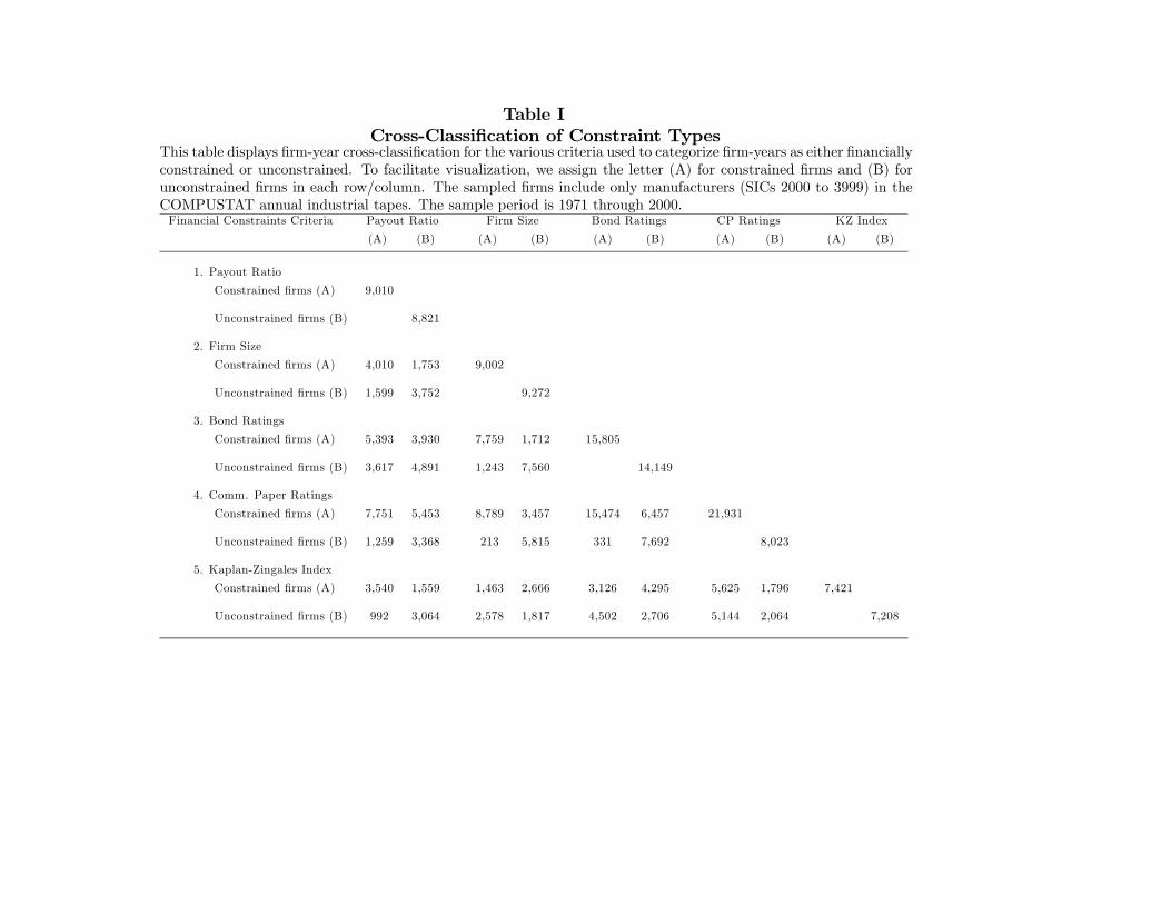
Table ICross-Classification of Constraint Types

This table displays firm-year cross-classification for the various criteria used to categorize firm-years as either financiallyconstrained or unconstrained. To facilitate visualization, we assign the letter (A) for constrained firms and (B) forunconstrained firms in each row/column. The sampled firms include only manufacturers (SICs 2000 to 3999) in theCOMPUSTAT annual industrial tapes. The sample period is 1971 through 2000.Financial Constraints Criteria Payout Ratio Firm Size Bond Ratings CP Ratings KZ Index

(A) (B) (A) (B) (A) (B) (A) (B) (A) (B)

1. Payout Ratio

Constrained firms (A) 9,010

Unconstrained firms (B) 8,821

2. Firm Size

Constrained firms (A) 4,010 1,753 9,002

Unconstrained firms (B) 1,599 3,752 9,272

3. Bond Ratings

Constrained firms (A) 5,393 3,930 7,759 1,712 15,805

Unconstrained firms (B) 3,617 4,891 1,243 7,560 14,149

4. Comm. Paper Ratings

Constrained firms (A) 7,751 5,453 8,789 3,457 15,474 6,457 21,931

Unconstrained firms (B) 1,259 3,368 213 5,815 331 7,692 8,023

5. Kaplan-Zingales Index

Constrained firms (A) 3,540 1,559 1,463 2,666 3,126 4,295 5,625 1,796 7,421

Unconstrained firms (B) 992 3,064 2,578 1,817 4,502 2,706 5,144 2,064 7,208

Table IISummary Statistics of Cash Holdings

This table displays summary statistics for cash holdings across groups offinancially constrained and unconstrained firms. We assign the letter (A)for constrained firms and (B) for unconstrained firms in each row. Alldata are from the annual COMPUSTAT industrial tapes. The sampledfirms include only manufacturers (SICs 2000 to 3999) and the sampleperiod is 1971 through 2000.

Cash Holdings Mean Median Std. Dev. N. Obs

Financial Constraints Criteria

1. Payout Ratio

Constrained firms (A) 0.145 0.074 0.177 9,010

Unconstrained firms (B) 0.090 0.051 0.106 8,821

p-value (A−B 6=0) 0.00 0.00

2. Firm Size

Constrained firms (A) 0.178 0.110 0.191 9,002

Unconstrained firms (B) 0.079 0.051 0.082 9,272

p-value (A−B 6=0) 0.00 0.00

3. Bond Ratings

Constrained firms (A) 0.146 0.085 0.167 15,805

Unconstrained firms (B) 0.081 0.049 0.092 14,149

p-value (A−B 6=0) 0.00 0.00

4. Comm. Paper Ratings

Constrained firms (A) 0.129 0.070 0.155 21,931

Unconstrained firms (B) 0.076 0.051 0.076 8,023

p-value (A−B 6=0) 0.00 0.00

5. Kaplan-Zingales Index

Constrained firms (A) 0.055 0.030 0.076 7,421

Unconstrained firms (B) 0.179 0.134 0.166 7,208

p-value (A−B 6=0) 0.00 0.00

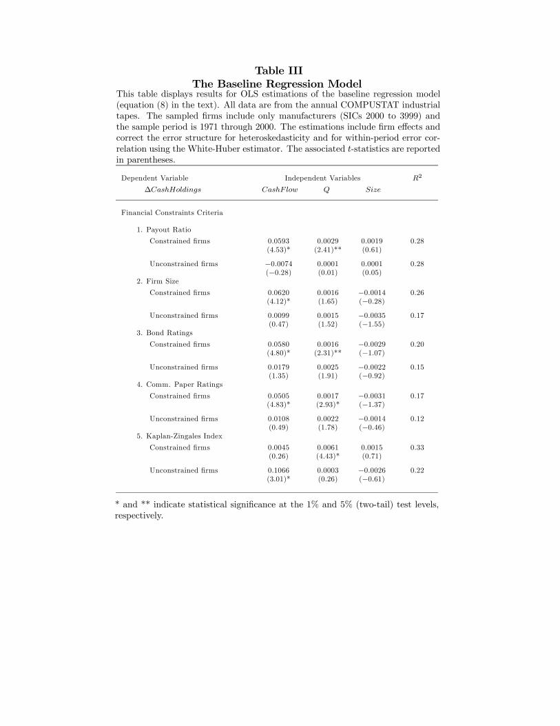
Table IIIThe Baseline Regression Model

This table displays results for OLS estimations of the baseline regression model(equation (8) in the text). All data are from the annual COMPUSTAT industrialtapes. The sampled firms include only manufacturers (SICs 2000 to 3999) andthe sample period is 1971 through 2000. The estimations include firm effects andcorrect the error structure for heteroskedasticity and for within-period error cor-relation using the White-Huber estimator. The associated t-statistics are reportedin parentheses.

Dependent Variable Independent Variables R2

∆CashHoldings CashF low Q Size

Financial Constraints Criteria

1. Payout Ratio

Constrained firms 0.0593 0.0029 0.0019 0.28(4.53)* (2.41)** (0.61)

Unconstrained firms −0.0074 0.0001 0.0001 0.28(−0.28) (0.01) (0.05)

2. Firm Size

Constrained firms 0.0620 0.0016 −0.0014 0.26(4.12)* (1.65) (−0.28)

Unconstrained firms 0.0099 0.0015 −0.0035 0.17(0.47) (1.52) (−1.55)

3. Bond Ratings

Constrained firms 0.0580 0.0016 −0.0029 0.20(4.80)* (2.31)** (−1.07)

Unconstrained firms 0.0179 0.0025 −0.0022 0.15(1.35) (1.91) (−0.92)

4. Comm. Paper Ratings

Constrained firms 0.0505 0.0017 −0.0031 0.17(4.83)* (2.93)* (−1.37)

Unconstrained firms 0.0108 0.0022 −0.0014 0.12(0.49) (1.78) (−0.46)

5. Kaplan-Zingales Index

Constrained firms 0.0045 0.0061 0.0015 0.33(0.26) (4.43)* (0.71)

Unconstrained firms 0.1066 0.0003 −0.0026 0.22(3.01)* (0.26) (−0.61)

* and ** indicate statistical significance at the 1% and 5% (two-tail) test levels,respectively.

Table IVThe Augmented RegressionModel

This table displays results for IV estimations of the augmented regression model (equation (9) in the text). All data are from theannual COMPUSTAT industrial tapes. The sampled firms include only manufacturers (SICs 2000 to 3999) and the sample period is1971 through 2000. The estimations include firm effects and correct the error structure for heteroskedasticity and for within-period errorcorrelation using the White-Huber estimator. The associated t-statistics are reported in parentheses.

Dependent Variable Independent Variables R2

∆CashHoldings CashF low Q Size Expenditures Acquisitions ∆NWC ∆ShortDebt

Financial Constraints Criteria

1. Payout Ratio

Constrained firms 0.1488 0.0103 0.0123 −0.6471 −0.5061 −0.0013 0.1196 0.11(1.86) (1.65) (1.11) (−0.92) −(0.53) (−4.35)* (1.05)

Unconstrained firms 0.0240 −0.0015 0.0608 −1.6137 −3.1656 −0.0004 0.5432 0.07(0.44) (−0.39) (2.75)* (−1.89) (−2.72)* (−1.92) (2.39)**

2. Firm Size

Constrained firms 0.3836 0.0118 0.0539 −1.2773 −0.1763 −0.0223 0.3735 0.15(12.24)* (5.22)* (5.05)* (−4.78)* (−0.70) (−14.27)* (4.78)*

Unconstrained firms 0.0364 0.0010 0.0179 0.0626 −0.7855 −0.0001 0.2435 0.12(1.08) (0.62) (3.12)* (0.25) (−2.74)* (−2.82)* (2.32)**

3. Bond Ratings

Constrained firms 0.2793 0.0073 0.0291 −1.1936 0.1016 −0.0051 0.2735 0.11(3.17)* (1.23) (1.26) (−1.63) (0.13) (−4.41)* (1.58)

Unconstrained firms −0.0975 0.0109 0.0358 −0.2179 −2.4192 −0.0001 0.1575 0.13(−1.81) (3.31)* (3.92)* (−0.64) (−3.68)* (−0.63) (1.41)

4. Comm. Paper Ratings

Constrained firms 0.3374 0.0127 0.0265 −1.6352 −0.2931 −0.0049 0.2443 0.12(5.13)* (3.51)* (2.16)** (−3.17)* (−0.53) (−6.11)* (2.42)**

Unconstrained firms −0.2777 0.0050 0.0330 0.6430 −1.6936 0.0001 0.0093 0.12(−2.13)** (1.93) (3.06)* (2.08)** (−2.43)** (0.49) (0.09)

5. Kaplan-Zingales Index

Constrained firms 0.1621 0.0080 −0.0097 −0.9989 0.0552 −0.0003 0.2937 0.10(1.97)** (1.60) (−0.88) (−2.52)** (0.13) (−3.02)* (2.28)**

Unconstrained firms 0.3053 0.0216 0.0398 −2.1115 0.2851 −0.0053 0.7159 0.09(3.40)* (2.27)** (1.32) (−1.33) (0.28) (−4.31)* (2.29)**

* and ** indicate statistical significance at the 1% and 5% (two-tail) test levels, respectively.

Table VRobustness Checks

This table shows results for alternative versions of the baseline model (equation (8)) and alternative sampling. Only thecoefficients returned for CashF low are reported. All data are from the annual COMPUSTAT industrial tapes. The sampledfirms include only manufacturers (SICs 2000 to 3999) from 1971 through 2000. The estimations include firm effects andcorrect the error structure for heteroskedasticity and for within-period error correlation using the White-Huber estimator.The associated t-statistics are reported in parentheses.

Dependent Variable Financial Constraints Criteria

∆CashHoldings Payout Ratio Firm Size Bond Ratings CP Ratings KZ Index

1. Sample restricted to firms with positive freecash flow

Constrained firms 0.0789 0.0889 0.0954 0.0966 0.0157(1.89) (2.40)** (3.58)* (4.39)* (0.43)

Unconstrained firms −0.1052 0.0520 0.0657 0.0062 0.1815(−2.32)** (1.05) (1.18) (0.11) (2.89)*

2. Q is replaced by the ratio of (realized) future investmentto current investment

Constrained firms 0.0450 0.0729 0.0614 0.0498 0.0020(2.35)** (3.17)* (3.22)* (3.57)* (0.09)

Unconstrained firms 0.0068 0.0090 0.0120 0.0044 0.1118(0.22) (0.58) (0.86) (0.27) (2.70)*

3. Q is instrumented with financial analysts’ earningsforecasts

Constrained firms 0.0447 0.0144 0.0568 0.0867 0.0496(3.50)* (0.71) (2.76)* (2.06)** (1.30)

Unconstrained firms −0.0091 0.0181 0.0255 0.0119 0.0950(−0.68) (0.98) (1.06) (0.72) (4.94)*

4. Lagged Cash/Assets and its interaction with CashFloware added to the r.h.s. of the model

Constrained firms 0.0621 0.1243 0.0431 0.0415 0.0021(2.63)* (3.80)* (1.98)** (2.96)* (0.07)

Unconstrained firms −0.0127 0.0178 0.0204 −0.0209 0.0597(−0.40) (1.01) (1.26) (−0.88) (2.26)**

* and ** indicate statistical significance at the 1% and 5% (two-tail) test levels, respectively.

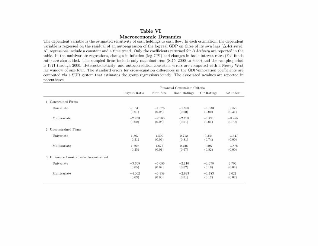
Table VIMacroeconomic Dynamics

The dependent variable is the estimated sensitivity of cash holdings to cash flow. In each estimation, the dependentvariable is regressed on the residual of an autoregression of the log real GDP on three of its own lags (∆Activity).All regressions include a constant and a time trend. Only the coefficients returned for ∆Activity are reported in thetable. In the multivariate regressions, changes in inflation (log CPI) and changes in basic interest rates (Fed fundsrate) are also added. The sampled firms include only manufacturers (SICs 2000 to 3999) and the sample periodis 1971 through 2000. Heteroskedasticity- and autocorrelation-consistent errors are computed with a Newey-Westlag window of size four. The standard errors for cross-equation differences in the GDP-innovation coefficients arecomputed via a SUR system that estimates the group regressions jointly. The associated p-values are reported inparentheses.

Financial Constraints Criteria

Payout Ratio Firm Size Bond Ratings CP Ratings KZ Index

1. Constrained Firms

Univariate −1.841 −1.576 −1.898 −1.333 0.156(0.01) (0.08) (0.00) (0.00) (0.31)

Multivariate −2.233 −2.283 −2.268 −1.491 −0.255(0.02) (0.08) (0.01) (0.01) (0.70)

2. Unconstrained Firms

Univariate 1.867 1.509 0.212 0.345 −3.547(0.31) (0.03) (0.81) (0.74) (0.00)

Multivariate 1.769 1.675 0.426 0.292 −3.876(0.25) (0.01) (0.67) (0.82) (0.00)

3. Difference Constrained−UnconstrainedUnivariate −3.708 −3.086 −2.110 −1.678 3.703

(0.05) (0.02) (0.02) (0.10) (0.01)

Multivariate −4.002 −3.958 −2.693 −1.783 3.621(0.03) (0.00) (0.01) (0.12) (0.02)