the capm and equity return - hillsdale inv

by Donald B. Keim

The CAPM and Equity Return Regularities

Differential returns on dividend and capital gains income, systematic abnormal returns surrounding ex-dividend dates, excess returns on small versus large capitalization stocks, excess returns on low versus high price-earnings ratio stocks-these are among the recent findings that cast doubt on the traditional Capital Asset Pricing Model and tease investors with the promise of systematic excess returns.

Some of these effects are undoubtedly related. Tests indicate, for example, that the higher a portfolio's price to book ratio, the higher the corresponding values of market capitalization, PIE and stock price. Furthermore, P/E, dividend yield, price and PIE effects all experience significant January seasonals. What has not been conclusively determined is whether the effects are additive. So far, it appears that the dividend yield and size effects are not mnutually exclusive. Investors may want to use a strategy employing several of these characteristics, rather than one.

Efforts to explain the size effect have focused on January, because the effect is concentrated in that month. The most common hypothesis attributes this to year-end tax-loss selling, but the evidence is less than conclusive. Evidence strongly suggests, however, that, among small firms, those with the largest abnormal returns tend to be the firms that have recently become small, that either don't pay dividends or have higher dividend yields, and that have lower prices and low PIE ratios.

T HE CAPITAL ASSET Pricing Model (CAPM) has occupied a central position in financial economics since its introduc-

tion over 20 years ago.' The CAPM states that, under certain simplifying assumptions, the rate of return on any asset may be expected to equal the rate of return on a riskless asset plus a premium that is proportional to the asset's risk relative to the market.2 This is expressed mathe- matically as follows:

E(R1) = Rz + [E(RM) - Rz]fi,

where E(Ri) = the expected rate of return on asset i;

Rz = rate of return on the riskless asset;3 E(RM) = the expected rate of return on the

market portfolio of all marketable assets; and

pi = the asset's sensitivity to market movements (beta).

If the model is correct, and security markets are efficient, security return will on average conform to the above relation.4 Persistent departures from the expected relation, however, may indicate that the CAPM and/or the Efficient Market Hypothesis are incorrect.5

The strict set of assumptions underlying the CAPM has prompted numerous criticisms. But any model proposes a simplified view of the world; that is not sufficient grounds for rejection. Rejection or acceptance should rest on scientific evidence. The University of Chicago's creation of a computerized database of stock prices and distributions in the 1960s made such

1. Footnotes appear at end of article.

Donald Keim is Assistant Professor of Finance at the Wharton School of the University of Pennsylvania.

The author thanks Wayne Ferson, Allan Kleidon, Craig MacKinlay, Terry Marsh, Krishna Ramaswamy and Jay Ritter for their helpful comments.

FINANCIAL ANALYSTS JOURNAL / MAY-JUNE 1986 O 19

The CFA Instituteis collaborating with JSTOR to digitize, preserve, and extend access to

Financial Analysts Journalwww.jstor.org

®

testing possible. This article reviews briefly some of the results of these tests and discusses in some detail more recent evidence that raises serious questions about the validity of the CAPM.

Early Evidence Numerous studies in the early 1970s generally supported the CAPM, although finding the coefficient on beta (representing an estimate of the market risk premium) to be only marginally important in explaining cross-sectional differ- ences in average security returns.6 In 1977, however, Roll raised some legitimate questions about the validity of these tests.7 Briefly, Roll argued that tests performed with any market portfolio other than the true market portfolio are not tests of the CAPM, and that tests of the CAPM may be extremely sensitive to the choice of market proxy. He also pointed out that some of the early tests' need to specify an alternative model to the CAPM may have led to faulty inferences. For instance, Fama and MacBeth had tested whether residual variance or beta squared help explain returns; thus the CAPM may be false, but if residual variance or beta squared do not capture the violation, the test will not reject the model.8

In response to Roll's first point, Stambaugh constructed broader market indexes that includ- ed bonds and real estate and found that such tests did not seem to be very sensitive to the choice of market proxy.9 Gibbons, Stambaugh and others have addressed Roll's second point by using multivariate tests that do not require the specification of an alternative asset pricing model. 10 These multivariate tests have not conclusively proved or disproved the validity of the CAPM.

Researchers have meanwhile formulated alternative models, many of which relax some of the CAPM assumptions. Mayers, for example, allowed for nonmarketable assets such as hu- man capital; Brennan and Litzenberger and Ra- maswamy relaxed the no-tax assumption." Others, in the spirit of Fama and MacBeth, have examined ad hoc alternatives to the CAPM. Among this group, Banz examined the importance of market value of common equity, and Basu investigated the importance of price-earnings ratios in explaining risk-adjusted returns. 12

The rest of this article discusses such alternatives to the CAPM and the implications of the associated evidence for portfolio management.

After-Tax Effects Because in the U.S. dividend income is subject to a higher marginal tax rate than capital gains, taxable investors should rationally prefer a dollar of pretax capital gain to a dollar of dividends. Brennan and Litzenberger and Ramaswamy extended the CAPM to include an extra factor- dividend yield. They hypothesized that, the higher a stock's dividend yield, holding risk constant, the higher the pretax return a taxable investor will require in order to compensate for the tax liability incurred.

There are, of course, counter arguments. Miller and Scholes argued that the tax code permits investors to transform dividend income into capital gains. 13 If the marginal investors are using these or other effective shelters, then the pretax rate on dividend-paying stocks may not differ from the rate on stocks that do not pay dividends. The tax differential has nevertheless prompted some tax-exempt institutions to "tilt" their portfolios toward higher-yielding securities, with the hope of capturing the benefits of the supposedly higher pretax returns.

The effectiveness of such a strategy, of course, hinges on how well after-tax models conform to reality. An after-tax CAPM has the following general form:

E(Rj) = ao + a1 pi + a2di, (2)

where di equals the dividend yield for security i and a2 represents an implicit tax coefficient that is independent of the level of the dividend yield. The question is whether a2 is reliably positive and consistent with realistic tax rates.

Empirical tests of the hypothesis that a2 equals zero face several difficulties. Because asset pricing models are cast in terms of expectations, the researcher needs to arrive at a suitable ex ante dividend yield measure. Fur- ther, he must ask whether the tax effects that motivate the model occur at a single point in time (i.e., the ex-dividend date), or whether they are spread over a longer period. Finally, most researchers have assumed a linear relation between dividend yields and returns, but the relation might be more complicated.

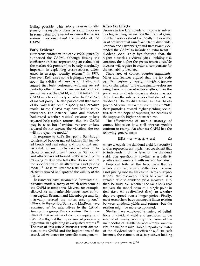
Studies have employed a variety of definitions of dividend yield and methods. In the interest of brevity, we forgo discussion of the methodological subtleties and simply summarize the major results. Table I reports estimates of the dividend yield coefficient a2.14 In each instance, the estimate of a2 is positive; holding

FINANCIAL ANALYSTS JOURNAL / MAY-JUNE 1986 C 20

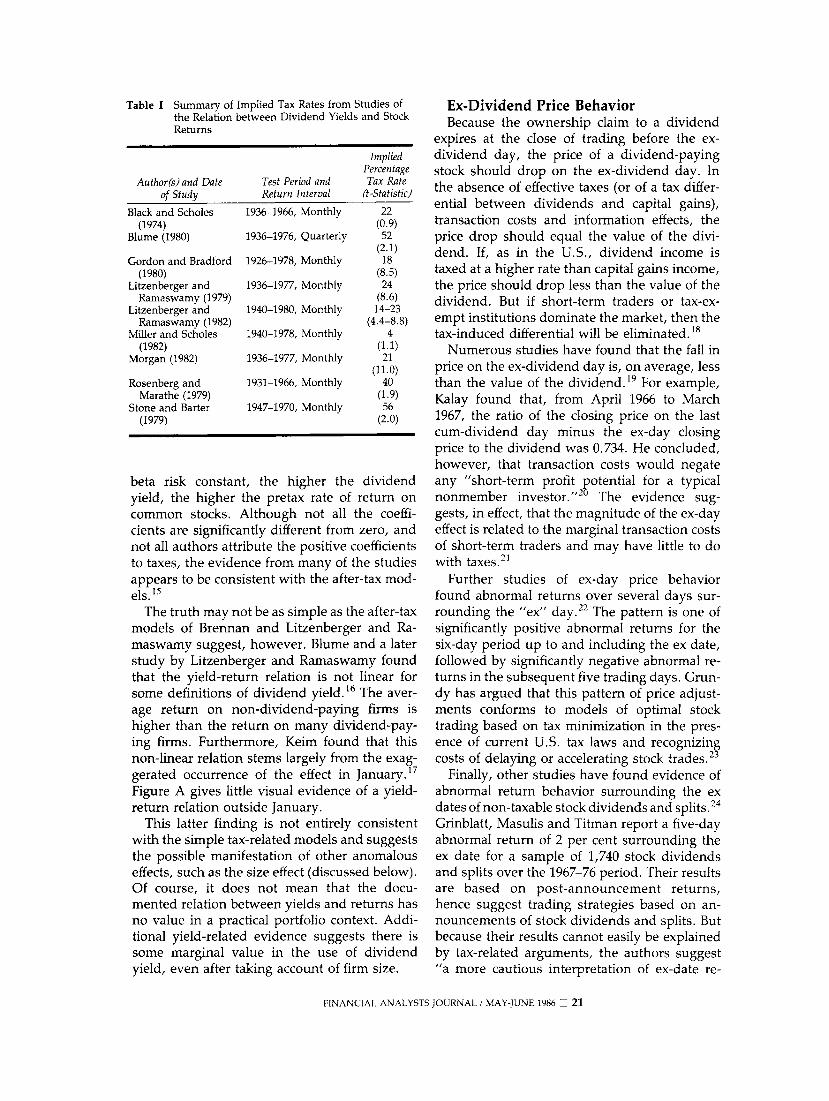
Table I Summary of Implied Tax Rates from Studies of the Relation between Dividend Yields and Stock Returns

Implied Percentage

Author(s) and Date Test Period and Tax Rate of Study Return Interval (t-Statistic)

Black and Scholes 1936-1966, Monthly 22 (1974) (0.9)

Blume (1980) 1936-1976, Quarterly 52 (2.1)

Gordon and Bradford 1926-1978, Monthly 18 (1980) (8.5)

Litzenberger and 1936-1977, Monthly 24 Ramaswamy (1979) (8.6)

Litzenberger and 1940-1980, Monthly 14-23 Ramaswamy (1982) (4.4-8.8)

Miller and Scholes 1940-1978, Monthly 4 (1982) (1.1)

Morgan (1982) 1936-1977, Monthly 21 (11.0)

Rosenberg and 1931-1966, Monthly 40 Marathe (1979) (1.9)

Stone and Barter 1947-1970, Monthly 56 (1979) (2.0)

beta risk constant, the higher the dividend yield, the higher the pretax rate of return on common stocks. Although not all the coefficients are significantly different from zero, and not all authors attribute the positive coefficients to taxes, the evidence from many of the studies appears to be consistent with the after-tax models. 15

The truth may not be as simple as the after-tax models of Brennan and Litzenberger and Ra- maswamy suggest, however. Blume and a later study by Litzenberger and Ramaswamy found that the yield-return relation is not linear for some definitions of dividend yield. 16 The average return on non-dividend-paying firms is higher than the return on many dividend-paying firms. Furthermore, Keim found that this non-linear relation stems largely from the exag- gerated occurrence of the effect in January.'7 Figure A gives little visual evidence of a yield- return relation outside January.

This latter finding is not entirely consistent with the simple tax-related models and suggests the possible manifestation of other anomalous effects, such as the size effect (discussed below). Of course, it does not mean that the documented relation between yields and returns has no value in a practical portfolio context. Addi- tional yield-related evidence suggests there is some marginal value in the use of dividend yield, even after taking account of firm size.

Ex-Dividend Price Behavior Because the ownership claim to a dividend

expires at the close of trading before the ex- dividend day, the price of a dividend-paying stock should drop on the ex-dividend day. In the absence of effective taxes (or of a tax differential between dividends and capital gains), transaction costs and information effects, the price drop should equal the value of the dividend. If, as in the U.S., dividend income is taxed at a higher rate than capital gains income, the price should drop less than the value of the dividend. But if short-term traders or tax-exempt institutions dominate the market, then the tax-induced differential will be eliminated. 18

Numerous studies have found that the fall in price on the ex-dividend day is, on average, less than the value of the dividend.'9 For example, Kalay found that, from April 1966 to March 1967, the ratio of the closing price on the last cum-dividend day minus the ex-day closing price to the dividend was 0.734. He concluded, however, that transaction costs would negate any "short-term profit potential for a typical nonmember investor."20 The evidence suggests, in effect, that the magnitude of the ex-day effect is related to the marginal transaction costs of short-term traders and may have little to do with taxes.2'

Further studies of ex-day price behavior found abnormal returns over several days surrounding the "ex" day.22 The pattern is one of significantly positive abnormal returns for the six-day period up to and including the ex date, followed by significantly negative abnormal returns in the subsequent five trading days. Grun- dy has argued that this pattern of price adjust- ments conforms to models of optimal stock trading based on tax minimization in the presence of current U.S. tax laws and recognizing costs of delaying or accelerating stock trades.23

Finally, other studies have found evidence of abnormal return behavior surrounding the ex dates of non-taxable stock dividends and splits.24 Grinblatt, Masulis and Titman report a five-day abnormal return of 2 per cent surrounding the ex date for a sample of 1,740 stock dividends and splits over the 1967-76 period. Their results are based on post-announcement returns, hence suggest trading strategies based on an- nouncements of stock dividends and splits. But because their results cannot easily be explained by tax-related arguments, the authors suggest "a more cautious interpretation of ex-date re-


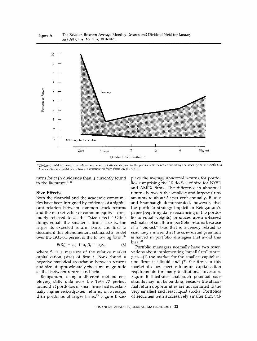
Figure A The Relation Between Average Monthly Returns and Dividend Yield for January and All Other Months, 1931-1978

10

9

8

7

6 January

r~ 5

4

Zero Lowest 2 3 4 Highest

Dividend Yield Portfolio*

., ~ ~ ~ ~ ~ ~ ~ ~ ~ ~ ~ ~ ~ ~ ~ ~ ~ ~ ~ ~ ~ ~ ~ ~ ~ ~ ~ ~ ~ ~ ~ ~ ~ ~ ~ ... ..

*Dividend yield in month t is defined as the sum of dividends paid in the previous 12 months divided by the stock price in month t-13. The six dividend yield portfolios are constructed from firms on the NYSE.

turns for cash dividends than is currently found in the literature."25

Size Effects Both the financial and the academic communi- ties have been intrigued by evidence of a significant relation between common stock returns and the market value of common equity-com- monly referred to as the "size effect." Other things equal, the smaller a firm's size is, the larger its expected return. Banz, the first to document this phenomenon, estimated a model over the 1931-75 period of the following form:26

E(R1) = ao + a, f3i + a2Si, (3)

where Si is a measure of the relative market capitalization (size) of firm i. Banz found a negative statistical association between returns and size of approximately the same magnitude as that between returns and beta.

Reinganum, using a different method employing daily data over the 1963-77 period, found that portfolios of small firms had substantially higher risk-adjusted returns, on average, than portfolios of larger firms.27 Figure B dis-

plays the average abnormal returns for portfolios comprising the 10 deciles of size for NYSE and AMEX firms. The difference in abnormal returns between the smallest and largest firms amounts to about 30 per cent annually. Blume and Stambaugh demonstrated, however, that the portfolio strategy implicit in Reinganum's paper (requiring daily rebalancing of the portfolio to equal weights) produces upward-biased estimates of small-firm portfolio returns because of a "bid-ask" bias that is inversely related to size; they showed that the size-related premium is halved in portfolio strategies that avoid this bias.28

Portfolio managers normally have two reser- vations about implementing "small firm" strategies-(1) the market for the smallest capitalization firms is illiquid and (2) the firms in this market do not meet minimum capitalization requirements for many institutional investors. Figure B illustrates that such potential constraints may not be binding, because the abnormal return opportunities are not confined to the very smallest and least liquid stocks. Portfolios of securities with successively smaller firm val-

FINANCIAL ANALYSTS JOURNAL / MAY-JUNE 1986 D 22

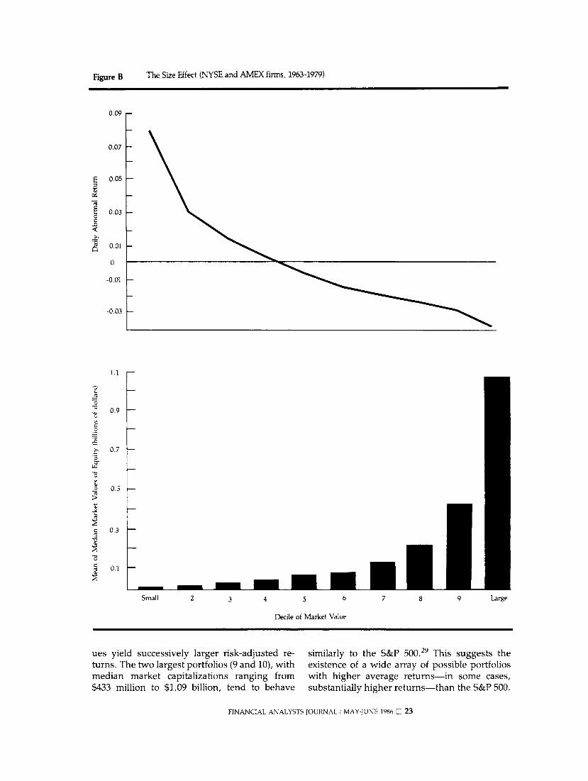
Figure B The Size Effect (NYSE and AMEX firms, 1963-1979)

0.09

0.07

: 0.05

0.03

0.01

0

-0.01

-0.03

1.1

0.9

>, 0.7

C)

- 0.5

0.3

r~0.1

Small 2 3 4 5 6 7 8 9 Large

Decile of Market Value

ues yield successively larger risk-adjusted returns. The two largest portfolios (9 and 10), with median market capitalizations ranging from $433 million to $1.09 billion, tend to behave

similarly to the S&P 500.29 This suggests the existence of a wide array of possible portfolios with higher average returns-in some cases, substantially higher returns-than the S&P 500.


Figure C Size Effect by Day of the Week (NYSE and AMEX firms, 1963-1979)

0.4 -

0.3 -

0.2

Tuesday

-0.1

Monday -0.2

Small 2 3 4 5 6 7 8 9 Large

Size Portfolio

Much subsequent research on the size effect has attempted to provide a more complete char- acterization of the phenomenon. We now know that, among the firms that academic researchers consider "small" (in 1980, the smallest size quintile for the NYSE represented firms with market capitalizations of less than about $50 million), those with the largest abnormal returns tend to be firms that have recently become small (or that have recently declined in price), that either do not pay a dividend or have high dividend yields, that have low prices, and that have low price-earnings ratios.30

Seasonal Size Effects Researchers have also examined the time-

related patterns of portfolio returns stratified by market capitalization. Brown, Kleidon and Marsh found that, when averaged over all months, the size effect reverses itself for sus- tained periods; in many periods there is a consistent premium for small size, whereas in other (fewer) periods there is a discount.3' In some periods (1969-73, for example), a small capitalization strategy would have underperformed the market on a beta-adjusted basis.

The magnitude of the size effect also seems to differ across days of the week and months of the year. Keim and Stambaugh found that the size effect becomes more pronounced as the week progresses and is most pronounced on Friday.32 Figure C shows that the negative relation between returns and size for the 1963-79 period becomes most pronounced at the end of the week.

The most dramatic seasonal pattern, however, involves the turn of the year. Keim found that the size effect is concentrated in January: Approximately 50 per cent of the return difference detected by Reinganum is concentrated in January.33 Figure D shows the extent to which this January seasonal affects the month-by- month behavior of the size effect. Keim also found that 50 per cent of this January effect is concentrated in the first five trading days of the year. This turn-of-the-year behavior was also detected by Roll, who noted abnormally large returns for small firms on the last trading day in December. 34

Researchers have also looked to international data to see whether the January seasonal pattern in the size effect that persists at the turn of


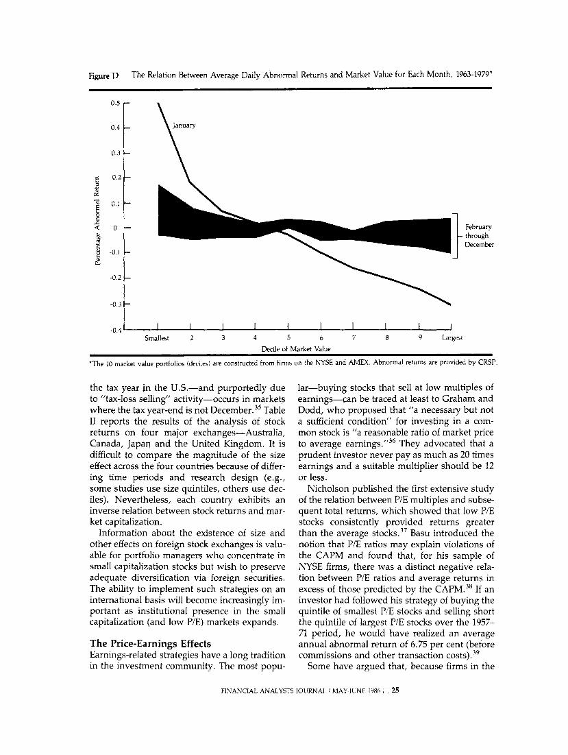
Figure D The Relation Between Average Daily Abnormal Returns and Market Value for Each Month, 1963-1979*

0.5

0.4 January

0.3

0.2

0.1

< 0 February through December

-0.1

-0.2

-0.3

-0.4 I l Smallest 2 3 4 5 6 7 8 9 Largest

Decile of Market Value

*The 10 market value portfolios (deciles) are constructed from firms on the NYSE and AMEX. Abnormal returns are provided by CRSP.

the tax year in the U.S-and purportedly due to "tax-loss selling" activity-occurs in markets where the tax year-end is not December.35 Table II reports the results of the analysis of stock returns on four major exchanges-Australia, Canada, Japan and the United Kingdom. It is difficult to compare the magnitude of the size effect across the four countries because of differ- ing time periods and research design (e.g., some studies use size quintiles, others use deciles). Nevertheless, each country exhibits an inverse relation between stock returns and market capitalization.

Information about the existence of size and other effects on foreign stock exchanges is valu- able for portfolio managers who concentrate in small capitalization stocks but wish to preserve adequate diversification via foreign securities. The ability to implement such strategies on an international basis will become increasingly important as institutional presence in the small capitalization (and low P/E) markets expands.

The Price-Earnings Effects Earnings-related strategies have a long tradition in the investment community. The most popu-

lar-buying stocks that sell at low multiples of earnings-can be traced at least to Graham and Dodd, who proposed that "a necessary but not a sufficient condition" for investing in a common stock is "a reasonable ratio of market price to average earnings."36 They advocated that a prudent investor never pay as much as 20 times earnings and a suitable multiplier should be 12 or less.

Nicholson published the first extensive study of the relation between P/E multiples and subsequent total returns, which showed that low P/E stocks consistently provided returns greater than the average stocks.37 Basu introduced the notion that P/E ratios may explain violations of the CAPM and found that, for his sample of NYSE firms, there was a distinct negative relation between P/E ratios and average returns in excess of those predicted by the CAPM.38 If an investor had followed his strategy of buying the quintile of smallest P/E stocks and selling short the quintile of largest P/E stocks over the 1957- 71 period, he would have realized an average annual abnormal return of 6.75 per cent (before commissions and other transaction costs).39

Some have argued that, because firms in the


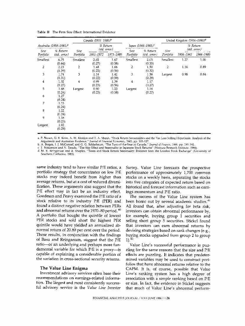
Table II The Firm Size Effect: International Evidence

Canada (1951_1980)b United Kingdom (1956-1980)d

Australia (1958-1981)a % Return Japan (1966-1983)C % Return

Size % Return Size (std. error) Size % Return Size (std. error) Portfolio (std. error) Portfolio 1951-1972 1973-1980 Portfolio (std. error) Portfolio 1956-1965 1966-1980

Smallest 6.75 Smallest 2.02 1.67 Smallest 2.03 Smallest 1.27 1.00 (0.64) (0.27) (0.58) (0.35)

2 2.23 2 1.48 1.66 2 1.50 2 1.18 0.89 (0.39) (0.22) (0.56) (0.32)

3 1.74 3 1.14 1.41 3 1.38 Largest 0.98 0.84 (0.31) (0.22) (0.59) (0.29)

4 1.32 4 0.99 1.39 4 1.17 (0.27) (0.23) (0.56) (0.27)

5 1.48 Largest 0.90 1.23 Largest 1.14 (0.24) (0.23) (0.58) (0.27)

6 1.27 (0.24)

7 1.15 (0.24)

8 1.22 (0.24)

9 1.18 (0.25)

Largest 1.02 (0.29)

a. P. Brown, D. B. Keim, A. W. Kleidon and T. A. Marsh, "Stock Return Seasonalities and the Tax Loss Selling Hypothesis: Analysis of the Arguments and Australian Evidence," Journal of Financial Economics, 1983, pp. 105-127.

b. A. Berges, J. J. McConnell and G. G. Schlarbaum, "The Turn-of-the-Year in Canada," Journal of Finance, 1984, pp. 185-192. c. T. Nakamura and N. Terada, "The Size Effect and Seasonality in Japanese Stock Returns" (Nomura Research Institute, 1984). d. M. R. Reinganum and A. Shapiro, "Taxes and Stock Return Seasonality: Evidence from the London Stock Exchange" (University of

Southern California, 1983).

same industry tend to have similar P/E ratios, a portfolio strategy that concentrates on low P/E stocks may indeed benefit from higher than average returns, but at a cost of reduced diversification. These arguments also suggest that the P/E effect may in fact be an industry effect. Goodman and Peavy examined the P/E ratio of a stock relative to its industry P/E (PER) and found a distinct negative relation between PERs and abnormal returns over the 1970-80 period.40 A portfolio that bought the quintile of lowest PER stocks and sold short the highest PER quintile would have yielded an annualized abnormal return of 20.80 per cent over the period. These results, in conjunction with the findings of Basu and Reinganum, suggest that the P/E ratio-or an underlying and perhaps more fundamental variable for which P/E is a proxy-is capable of explaining a considerable portion of the variation in cross-sectional security returns.

The Value Line Enigma Investment advisory services often base their

recommendations on earnings-related information. The largest and most consistently successful advisory service is the Value Line Investor

Survey. Value Line forecasts the prospective performance of approximately 1,700 common stocks on a weekly basis, separating the stocks into five categories of expected return based on historical and forecast information such as earnings momentum and P/E ratio.

The success of the Value Line system has been borne out by several academic studies.4' All found that, after adjusting for beta risk, investors can obtain abnormal performance by, for example, buying group 1 securities and selling short group 5 securities. Stickel found that investors can earn abnormal returns by devising strategies based on rank changes (e.g., buying stocks upgraded from group 2 to group i).42

Value Line's successful performance is puzzling for the same reasons that the size and P/E effects are puzzling. It indicates that predeter- mined variables may be used to construct portfolios that have abnormal returns relative to the CAPM. It is, of course, possible that Value Line's ranking system has a high degree of association with a simple ranking based on P/E or size. In fact, the evidence in Stickel suggests that much of Value Line's abnormal perform-


ance might be attributable to a small firm effect. More research is necessary to sort out these issues.

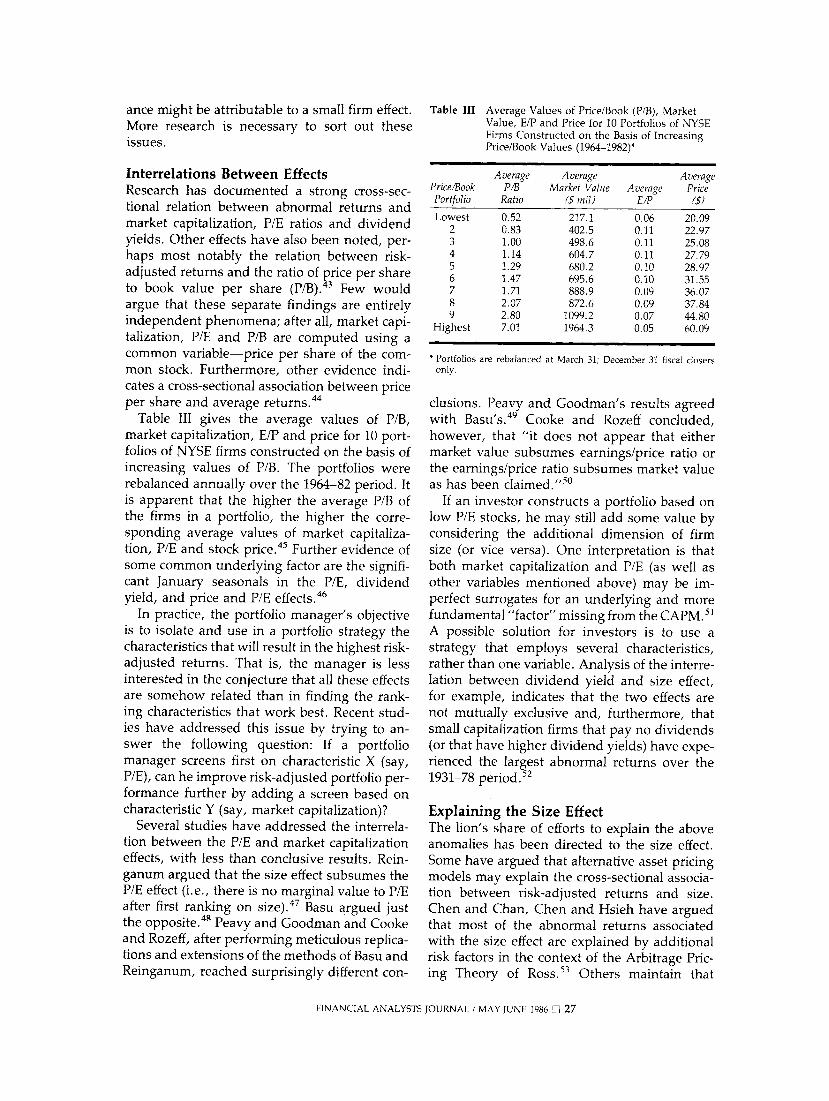
Interrelations Between Effects Research has documented a strong cross-sectional relation between abnormal returns and market capitalization, P/E ratios and dividend yields. Other effects have also been noted, perhaps most notably the relation between risk- adjusted returns and the ratio of price per share to book value per share (P/B).43 Few would argue that these separate findings are entirely independent phenomena; after all, market capitalization, P/E and P/B are computed using a common variable-price per share of the common stock. Furthermore, other evidence indicates a cross-sectional association between price per share and average returns.44

Table III gives the average values of P/B, market capitalization, E/P and price for 10 portfolios of NYSE firms constructed on the basis of increasing values of P/B. The portfolios were rebalanced annually over the 1964-82 period. It is apparent that the higher the average P/B of the firms in a portfolio, the higher the corresponding average values of market capitalization, P/E and stock price.45 Further evidence of some common underlying factor are the significant January seasonals in the P/E, dividend yield, and price and P/E effects.46

In practice, the portfolio manager's objective is to isolate and use in a portfolio strategy the characteristics that will result in the highest risk- adjusted returns. That is, the manager is less interested in the conjecture that all these effects are somehow related than in finding the ranking characteristics that work best. Recent studies have addressed this issue by trying to an- swer the following question: If a portfolio manager screens first on characteristic X (say, P/E), can he improve risk-adjusted portfolio performance further by adding a screen based on characteristic Y (say, market capitalization)?

Several studies have addressed the interrela- tion between the P/E and market capitalization effects, with less than conclusive results. Rein- ganum argued that the size effect subsumes the P/E effect (i.e., there is no marginal value to P/E after first ranking on size).47 Basu argued just the opposite.48 Peavy and Goodman and Cooke and Rozeff, after performing meticulous replica- tions and extensions of the methods of Basu and Reinganum, reached surprisingly different con-

clusions. Peavy and Goodman's results agreed with Basu's.49 Cooke and Rozeff concluded, however, that "it does not appear that either market value subsumes earnings/price ratio or the earnings/price ratio subsumes market value as has been claimed."50

If an investor constructs a portfolio based on low P/E stocks, he may still add some value by considering the additional dimension of firm size (or vice versa). One interpretation is that both market capitalization and P/E (as well as other variables mentioned above) may be im- perfect surrogates for an underlying and more fundamental "factor" missing from the CAPM.5 A possible solution for investors is to use a strategy that employs several characteristics, rather than one variable. Analysis of the interre- lation between dividend yield and size effect, for example, indicates that the two effects are not mutually exclusive and, furthermore, that small capitalization firms that pay no dividends (or that have higher dividend yields) have experienced the largest abnormal returns over the 1931-78 period.52

Explaining the Size Effect The lion's share of efforts to explain the above anomalies has been directed to the size effect. Some have argued that alternative asset pricing models may explain the cross-sectional association between risk-adjusted returns and size. Chen and Chan, Chen and Hsieh have argued that most of the abnormal returns associated with the size effect are explained by additional risk factors in the context of the Arbitrage Pric- ing Theory of Ross.53 Others maintain that

Table III Average Values of Price/Book (P/B), Market Value, E/P and Price for 10 Portfolios of NYSE Firms Constructed on the Basis of Increasing Price/Book Values (1964-1982)*

Average Average Average Price/Book P/B Market Value Average Price Portfolio Ratio ($ mil) E/P ($)

Lowest 0.52 217.1 0.06 20.09 2 0.83 402.5 0.11 22.97 3 1.00 498.6 0.11 25.08 4 1.14 604.7 0.11 27.79 5 1.29 680.2 0.10 28.97 6 1.47 695.6 0.10 31.55 7 1.71 888.9 0.09 36.07 8 2.07 872.6 0.09 37.84 9 2.80 1099.2 0.07 44.80

Highest 7.01 1964.3 0.05 60.09

* Portfolios are rebalanced at March 31; December 31 fiscal closers only.


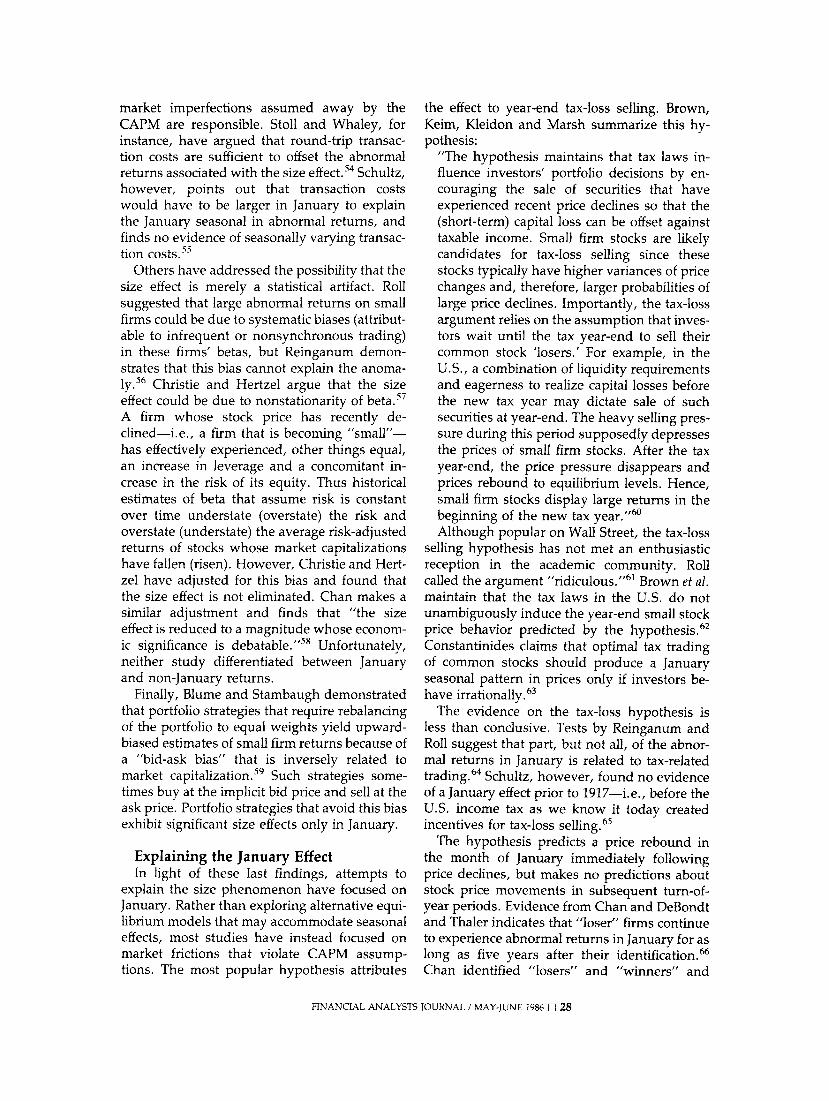
market imperfections assumed away by the CAPM are responsible. Stoll and Whaley, for instance, have argued that round-trip transaction costs are sufficient to offset the abnormal returns associated with the size effect.54 Schultz, however, points out that transaction costs would have to be larger in January to explain the January seasonal in abnormal returns, and finds no evidence of seasonally varying transaction costs.55

Others have addressed the possibility that the size effect is merely a statistical artifact. Roll suggested that large abnormal returns on small firms could be due to systematic biases (attributable to infrequent or nonsynchronous trading) in these firms' betas, but Reinganum demon- strates that this bias cannot explain the anomaly.56 Christie and Hertzel argue that the size effect could be due to nonstationarity of beta.57 A firm whose stock price has recently declined-i.e., a firm that is becoming "small"- has effectively experienced, other things equal, an increase in leverage and a concomitant increase in the risk of its equity. Thus historical estimates of beta that assume risk is constant over time understate (overstate) the risk and overstate (understate) the average risk-adjusted returns of stocks whose market capitalizations have fallen (risen). However, Christie and Hert- zel have adjusted for this bias and found that the size effect is not eliminated. Chan makes a similar adjustment and finds that "the size effect is reduced to a magnitude whose economic significance is debatable."58 Unfortunately, neither study differentiated between January and non-January returns.

Finally, Blume and Stambaugh demonstrated that portfolio strategies that require rebalancing of the portfolio to equal weights yield upward- biased estimates of small firm returns because of a "bid-ask bias"' that is inversely related to market capitalization.59 Such strategies some- times buy at the implicit bid price and sell at the ask price. Portfolio strategies that avoid this bias exhibit significant size effects only in January.

Explaining the January Effect In light of these last findings, attempts to

explain the size phenomenon have focused on January. Rather than exploring alternative equilibrium models that may accommodate seasonal effects, most studies have instead focused on market frictions that violate CAPM assumptions. The most popular hypothesis attributes

the effect to year-end tax-loss selling. Brown, Keim, Kleidon and Marsh summarize this hypothesis:

"The hypothesis maintains that tax laws influence investors' portfolio decisions by en- couraging the sale of securities that have experienced recent price declines so that the (short-term) capital loss can be offset against taxable income. Small firm stocks are likely candidates for tax-loss selling since these stocks typically have higher variances of price changes and, therefore, larger probabilities of large price declines. Importantly, the tax-loss argument relies on the assumption that investors wait until the tax year-end to sell their common stock 'losers.' For example, in the U.S., a combination of liquidity requirements and eagerness to realize capital losses before the new tax year may dictate sale of such securities at year-end. The heavy selling pressure during this period supposedly depresses the prices of small firm stocks. After the tax year-end, the price pressure disappears and prices rebound to equilibrium levels. Hence, small firm stocks display large returns in the beginning of the new tax year."60 Although popular on Wall Street, the tax-loss

selling hypothesis has not met an enthusiastic reception in the academic community. Roll called the argument "ridiculous.",61 Brown et al. maintain that the tax laws in the U.S. do not unambiguously induce the year-end small stock price behavior predicted by the hypothesis.62 Constantinides claims that optimal tax trading of common stocks should produce a January seasonal pattern in prices only if investors behave irrationally.63

The evidence on the tax-loss hypothesis is less than conclusive. Tests by Reinganum and Roll suggest that part, but not all, of the abnormal returns in January is related to tax-related trading.64 Schultz, however, found no evidence of a January effect prior to 1917-i.e., before the U.S. income tax as we know it today created incentives for tax-loss selling.65

The hypothesis predicts a price rebound in the month of January immediately following price declines, but makes no predictions about stock price movements in subsequent turn-of- year periods. Evidence from Chan and DeBondt and Thaler indicates that "loser" firms continue to experience abnormal returns in January for as long as five years after their identification.66 Chan identified "losers" and "winners" and


Figure E January Returns, Tax-Loss Portfolios (portfolios formed in December, year t)

7

6 - Year t+3

Year t + 1

5 - Year t+2

4

3

E

_ 2

-1I I I I I I I 1

Small 2 3 4 5 6 7 8 9 Large

Tax-Loss Portfolio

constructed an "arbitrage" portfolio (long losers, short winners) within each decile of market value for NYSE firms at December 31 of year t and tracked January abnormal returns in each of the following four years (t + 1 to t + 4). His results, presented in Figure E, show a persistent January effect in each of the subsequent three years. Based on such evidence, both Chan and Debondt and Thaler concluded that the January seasonal in stock returns may have little to do with tax-loss selling.

Others have tested the hypothesis by examining the month to month behavior of abnormal returns in countries with tax codes similar to the U.S. code but with different tax year-ends. They have found seasonals after the tax year-end, but also in January-a result not predicted by the hypothesis.67 Berges, McConnell and Schlar- baum found a January seasonal in Canadian stock returns prior to 1972-a period when Canada had no taxes on capital gains.68

The inconsistent evidence argues for investi- gating other possibilities. One that has received attention on Wall Street is the notion that liquidity constraints on market participants may influence security returns in a seasonal fashion. For example, periodic infusions of cash into the

market as a result of say, institutional transfers for pension accounts or proceeds from bonuses or profit-sharing plans may affect the market. Some evidence may be interpreted as support- ing this idea.

Kato and Schallheim, examining small firm returns in Japan, found January and June seasonals coinciding with the traditional bonuses paid at the end of December and in June.69 Rozeff found a substantial upward shift in the ratio of sales to purchases by investors who are not members of the NYSE coinciding with the dramatic increase in small firm returns in Janu- ary; Rozeff, however, interpreted this as evidence of a tax-loss selling effect.70 Ritter documented a similar pattern in the daily sales to purchase ratios for the retail customers of a large brokerage firm.7' And Ariel noted a pattern in daily stock returns in every month but February that parallels precisely the pattern that occurs at the turn of the year.72 It would be easier to interpret such monthly patterns as liquidity or payroll effects than as tax effects.

Other Seasonal Patterns Recent studies have documented additional

empirical regularities related to the day of the

FINANCIAL ANALYSTS JOURNAL / MAY-JUNE 1986 D 29

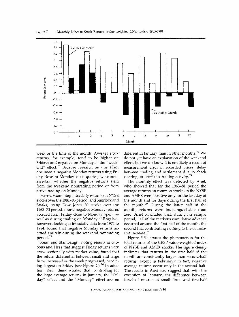
Figure F Monthly Effect in Stock Returns (value-weighted CRSP index, 1963-1981)

1.6

1.4 First Half of Month

1.2

0.8

0.6

0.4

S 0.2

0

-0.2

-0.4

-0.6 Last Half of Month

-0.8

-1.0

-1.2 1 2 3 4 5 6 7 8 9 10 11 12

Month

week or the time of the month. Average stock returns, for example, tend to be higher on Fridays and negative on Mondays-the "weekend" effect.73 Because research on this effect documents negative Monday returns using Fri- day close to Monday close quotes, we cannot ascertain whether the negative returns stem from the weekend nontrading period or from active trading on Monday.

Harris, examining intradaily returns on NYSE stocks over the 1981-83 period, and Smirlock and Starks, using Dow Jones 30 stocks over the 1963-73 period, found negative Monday returns accrued from Friday close to Monday open, as well as during trading on Monday.74 Rogalski, however, looking at intradaily data from 1974 to 1984, found that negative Monday returns accrued entirely during the weekend nontrading period. 75

Keim and Stambaugh, noting results in Gib- bons and Hess that suggest Friday returns vary cross-sectionally with market value, found that the return differential between small and large firms increased as the week progressed, becoming largest on Friday (see Figure C).76 In addi- tion, Keim demonstrated that, controlling for the large average returns in January, the "Fri- day" effect and the "Monday" effect are no

different in January than in other months.77 We do not yet have an explanation of the weekend effect, but we do know it is not likely a result of measurement error in recorded prices, delay between trading and settlement due to check clearing, or specialist trading activity.78

The monthly effect was detected by Ariel, who showed that for the 1963-81 period the average returns on common stocks on the NYSE and AMEX were positive only for the last day of the month and for days during the first half of the month.79 During the latter half of the month, returns were indistinguishable from zero. Ariel concluded that, during his sample period, "all of the market's cumulative advance occurred around the first half of the month, the second half contributing nothing to the cumulative increase."

Figure F illustrates the phenomenon for the total returns of the CRSP value-weighted index of NYSE and AMEX stocks. The figure clearly indicates that returns in the first half of the month are consistently larger than second-half returns (except in February); in fact, negative average returns occur only in the second half. The results in Ariel also suggest that, with the exception of January, the difference between first-half returns of small firms and first-half


returns of large firms is not substantial. Ariel is unable to explain the effect, but a potential explanation involves liquidity constraints.

Implications Many of these findings are inconsistent with an investment environment where the CAPM is descriptive of reality and argue for consider- ation of alternative models of asset pricing. Other findings, such as the day of the week effect, do not necessarily represent violations of any particular asset pricing model, yet are still intriguing because of their regularity.

The bottom line for portfolio managers is the extent to which this information can be translat- ed into improved portfolio performance. That strategies based on this evidence can improve performance has, in fact, been borne out in "real world" experiments. There are, however, several caveats regarding implementation of such strategies.

First, that some effects have persisted for as many as 50 years in no way guarantees their persistence into the future. Second, even if the effects were to persist, the costs of implementing strategies designed to capture these phenomena may be prohibitive. Market illiquidity and transaction costs may render a small stock strategy infeasible, for example. Day of the week and other seasonal effects may have practical value only for those investors who were planning to trade (and pay transaction costs) in any event.

Finally, one must be cautious when interpreting the magnitudes of "abnormal" returns found by the studies. To the extent that alternative models of asset pricing may be more appro- priate than the CAPM, studies that use the CAPM as a benchmark may not be adjusting completely for relevant risks and costs. Superior performance relative to the CAPM may not be superior once these costs and risks are consi- dered. E

Footnotes 1. See W. F. Sharpe, "Capital Asset Prices: A The-

ory of Market Equilibrium under Conditions of Risk," Journal of Finance 1964, pp. 425-442; J. Lintner, "The Valuation of Risk Assets and the Selection of Risky Investments in Stock Portfolios and Capital Budgets," Review of Economics and Statistics 1965, pp. 13-37; and J. L. Treynor, "Toward a Theory of Market Value of Risky Assets."

2. The one-period CAPM assumes that (1) investors are risk-averse and choose "efficient" portfolios by maximizing expected return for a given level of risk; (2) there are no taxes or transaction costs; (3) there are identical borrowing and lending rates; (4) investors are in complete agreement with regard to expectations about individual securities; and (5) security returns have a multivariate normal distribution.

3. Rz is the rate of return on a risk-free asset in the Sharpe-Lintner-Treynor CAPM; or the rate of return of an asset with zero correlation with the market in the extension by F. Black, "Capital Market Equilibrium with Restricted Borrowing," Journal of Business, July 1972, pp. 444-455.

4. See E. Fama, "Efficient Capital Markets: A Re- view of Theory and Empirical Work," Journal of Finance, May 1970, pp. 383-417.

5. Such persistent departures are often referred to as "anomalies." The term anomaly, in this context, can be traced to Thomas Kuhn in his classic book, The Structure of Scientific Revolutions (Chica- go: University of Chicago Press, 1970). Kuhn

maintains that research activity in any normal science will revolve around a central paradigm and that experiments are conducted to test the predictions of the underlying paradigm and to extend the range of the phenomena it explains. Although research most often supports the underlying paradigm, eventually results are found that don't conform. Kuhn terms this stage "discovery": "Discovery commences with the aware- ness of anomaly, i.e., with the recognition that nature has somehow violated the paradigm-induced expectations that govern normal science" (pp. 52-53, emphasis added).

6. The most prominent early studies are those of Black, Jensen and Scholes, "The Capital Asset Pricing Model: Some Empirical Evidence," in Jensen, ed., Studies in the Theory of Capital Markets (New York: Praeger, 1972); M. Blume and I. Friend, "A New Look at the Capital Asset Pricing Model," Journal of Finance, March 1973, pp. 19-33; and E. Fama and J. MacBeth, "Risk, Return and Equilibrium: Empirical Tests," Journal of Political Economy, May/June 1973, pp. 607-636.

7. R. Roll, "A Critique of the Asset Pricing Theory's Tests: Part I: On Past and Potential Testability of the Theory," Journal of Financial Economics, March 1977, pp. 129-176.

8. See Fama and MacBeth, "Risk, Return aned Equi- librium," op. cit.

9. R. Stambaugh, "On the Exclusion of Assets from the Two-Parameter Model: A Sensitivity Analy- sis," Journal of Financial Economics 1982, pp. 237- 268.


10. See M. Gibbons, "Multivariate Tests of Financial Models: A New Approach," Journal of Financial Economics 1982, pp. 3-27, and Stambaugh, "On the Exclusion," op. cit.

11. See D. Mayers, "Nonmarketable Assets and Cap- ital Market Equilibrium under Uncertainty," in Jensen, ed., Studies in Theory of Capital Markets, op cit.; M. Brennan, "Taxes, Market Valuation and Corporate Financial Policy," National Tax Journal 1970, pp. 417-427; and R. Litzenberger and K. Ramaswamy, "The Effects of Personal Taxes and Dividends on Capital Asset Prices: Theory and Empirical Evidence," Journal of Financial Economics 1979, pp. 163-195.

12. See R. W. Banz, "The Relationship between Return and Market Value of Common Stock," Journal of Financial Economics 1981, pp. 3-18, and S. Basu, "Investment Performance of Common Stocks in Relation to their Price/Earnings Ratios: A Test of the Efficient Market Hypothesis," Jour- nal of Finance 1977, pp. 663-682.

13. M. Miller and M. Scholes, "Dividends and Tax- es," Journal of Financial Economics, December 1978, pp. 333-364.

14. The table is an updated version of one in R. Litzenberger and K. Ramaswamy, "The Effects of Dividends on Common Stock Prices: Tax Effects or Information Effects," Journal of Finance 1982, pp. 429-433.

15. Coefficients are not significantly different from zero in findings by F. Black and M. Scholes, "The Effects of Dividend Yield and Dividend Policy on Common Stock Prices and Returns," Journal of Financial Economics 1974, pp. 1-22 and Miller and Scholes, "Dividends and Taxes: Some Empirical Evidence," Journal of Political Economy 1982, pp. 1118-1141. M. E. Blume ("Stock Returns and Dividend Yields: Some More Evidence," Review of Economics and Statistics 1980, pp. 567-577) and R.H. Gordon and D. F. Bradford ("Taxation and the Stock Market Valuation of Capital Gains and Dividends: Theory and Empirical Results," Jour- nal of Public Economics 1980, pp. 109-136) do not attribute the effects to taxes.

16. See Blume, "Stock Returns and Dividend Yields," op. cit. and R. Litzenberger and K. Ramaswamy, "Dividends, Short Selling Restric- tions, Tax-Induced Investor Clienteles and Mar- ket Equilibrium," Journal of Finance 1980, pp. 469-482.

17. See D.B. Keim, "Dividend Yields and Stock Re- turns: Implications of Abnormal January Re- turns," Journal of Financial Economics 1985, pp. 473-489, and Keim "Dividends Yields and the January Effect," Journal of Portfolio Management, 1986, pp. 61-65.

18. Except that transaction costs may keep the price from falling by the full amount of the dividend;

see Miller and Scholes, "Dividends and Taxes: Some Empirical Evidence," op. cit.

19. See, for example, J. Campbell and W. Berenek, "Stock Price Behavior on Ex-Dividend Dates," Journal of Finance 1953, pp. 425-429 and E. Elton and M. Gruber, "Marginal Stockholder Tax Rates and the Clientele Effect," Review of Economics and Statistics 1970, pp. 68-74.

20. A. Kalay, "The Ex-Dividend Day Behavior of Stock Prices: A Re-Examination of the Clientele Effect," Journal of Finance 1982, pp. 1059-1070.

21. For similar arguments, see K.M. Eades, P.J. Hess and E.H. Kim, "On Interpreting Returns During the Ex-Dividend Period," Journal of Financial Eco- nomics, March 1984, pp. 3-34. However, M. J. Barclay ("Tax Effects with No Taxes? Further Evidence on the Ex-Dividend Day Behavior of Common Stock Prices" (Department of Econom- ics, Stanford University, September 1984)) finds that in the period before the institution of the federal income tax, stock prices fell on their ex- dividend day by the full amount of the dividend. This evidence is suggestive of a tax story.

22. See F. Black and M. Scholes, "The Behavior of Security Returns Around Ex-Dividend Days" (University of Chicago, 1973); Eades, Hess and Kim, "On Interpreting Returns," op. cit.; and B. Grundy, "Trading Volume and Stock Returns around Ex-Dividend Dates" (University of Chica- go, 1985).

23. B. Grundy, "Trading Volume," op. cit. 24. See, for example, Eades, Hess and Kim, "On

Interpreting Returns," op. cit. and M. S. Grin- blatt, R.W. Masulis and S. Titman, "The Valuation Effects of Stock Splits and Stock Dividends," Journal of Financial Economics, December 1984, pp. 461-490.

25. Grinblatt, Masulis and Titman, "The Valuation Effects," op. cit.

26. Banz, "The Relationship Between Return and Market Value," op. cit.

27. M. R. Reinganum, "Misspecification of Capital Asset Pricing: Empirical Anomalies Based on Earnings' Yields and Market Values," Journal of Financial Economics 1981, pp. 19-46.

28. M. E. Blume and R. F. Stambaugh, "Biases in Computed Returns: An Application to the Size Effect," Journal of Financial Economics, November 1983, pp. 371-386.

29. The S&P 500, being a value-weighted index of primarily high-capitalization firms, behaves very much like a portfolio of very large firms.

30. The dividend influence is examined in Keim, "Dividend Yields and the January Effect, op. cit.; see H. R. Stoll and R.E. Whaley, "Transactions Costs and the Small Firm Effect," Journal of Finan- cial Economics, June 1983, pp. 57-80 and Blume and Stambaugh, "Biases in Computed Returns,"

FINANCIAL ANALYSTS JOURNAL / MAY-JUNE 1986 E 32

op. cit., for the effect of price; and Reinganum, "Misspecification of Capital Asset Pricing," op. cit., for the effect of low P/E.

31. P. Brown, A. W. Kleidon and T. A. Marsh, "New Evidence on the Nature of Size-Related Anoma- lies in Stock Prices," Journal of Financial Economics, June 1983, pp. 33-56.

32. D. B. Keim and R. F. Stambaugh, "A Further Investigation of the Weekend Effect in Stock Returns," Journal of Finance, July 1984, pp. 819- 835.

33. See D. B. Keim, "Size-Related Anomalies and Stock Return Seasonality: Further Empirical Evi- dence," Journal of Financial Economics, June 1983, pp. 13-32.

34. R. Roll, "Vas ist das? The Turn of the Year Effect and the Return Premium of Small Firms," Journal of Portfolio Management, 1983, pp. 18-28.

35. One exception is T. Nakamura and N. Terada ("The Size Effect and Seasonality in Japanese Stock Returns" (Nomura Research Institute, 1984) ), who document a P/E effect on the Tokyo stock exchange.

36. B. Graham and D. L. Dodd, Security Analysis (New York: McGraw-Hill, 1940), p. 533.

37. S. F. Nicholson, "Price-Earnings Ratios," Finan- cial Analysts Journal, July/August 1960.

38. Basu, "Investment Performance of Common Stocks," op. cit.

39. Reinganum ("Misspecification of Capital Asset Pricing," op. cit.), analyzing both NYSE and AMEX firms, confirmed and extended Basu's findings using return data to 1975.

40. J. W. Peavy and D. A. Goodman, "Industry- Relative Price-Earnings Ratios as Indicators of Investment Returns," Financial Analysts Journal, July/August 1983.

41. See, for example, F. Black, "Yes, Virginia, There is Hope: Tests of the Value Line Ranking Sys- tem," Financial Analysts Journal, September/Octo- ber 1973, pp. 10-14; C. Holloway, "A Note on Testing an Aggressive Investment Strategy Using Value Line Ranks," Journal of Finance, June 1981, pp. 711-719; and T. E. Copeland and D. Mayers, "The Value Line Enigma (1965-1978): A Case Study of Performance Evaluation Issues," Journal of Financial Economics, November 1982, pp. 289- 321.

42. S. E. Stickel, "The Effect of Value Line Investment Survey Rank Changes on Common Stock Prices," Journal of Financial Economics 1985, pp. 121-144.

43. Discussed most recently by B. Rosenberg, K. Reid and R. Lanstein, "Persuasive Evidence of Market Inefficiency," Journal of Portfolio Manage- ment, pp. 9-17.

44. See M E. Blume and F. Husic, "Price, Beta and Exchange Listing," Journal of Finance 1973, pp. 283-299; Stoll and Whaley, "Transactions Costs

and the Small Firm Effect," op. cit.; and Blume and Stambaugh, "Biases in Computed Returns," op. cit.

45. One exception is the lowest P/B portfolio, whose stocks on average have a low (high) average E/P (P/E). This is attributable to the negative earnings firms that tend to be concentrated there. Note that firms with negative book values are excluded from the sample.

46. For P/E, see T. J. Cooke and M. S. Rozeff, "Size and Earnings/Price Ratio Anomalies: One Effect or Two?" Journal of Financial and Quantitative Anal- ysis 1984, pp. 449-466; for dividend yield, see Keim, "Dividend Yields and Stock Returns," op. cit.; and for price, see J. Jaffe, D. Keim and R. Westerfield, "Disentangling Earnings/Price, Size and Other (related) Anomalies" (University of Pennsylvania, 1985).

47. See Reinganum, "Misspecification of Capital As- set Pricing," op. cit.

48. S. Basu, "The Relationship Between Earnings' Yields, Market Value and the Returns for NYSE Stocks: Further Evidence," Journal of Financial Economics, June 1983, pp. 129-156.

49. J. W. Peavy and D. A. Goodman, "A Further Inquiry into the Market Value and Earnings Yield Anomalies" (Southern Methodist University, 1982).

50. Cooke and Rozeff, "Size and Earnings/Price Ratio Anomalies," op. cit., p. 464.

51. See for example R. Ball, "Anomalies in Relation- ships between Securities' Yields and Yield-Surro- gates," Journal of Financial Economics 1978, pp. 108-126.

52. See Keim, "Dividend Yields and Stock Returns," op. cit. and "Dividend Yields and the January Effect," op. cit.

53. N. Chen, "Some Empirical Tests of the Theory of Arbitrage Pricing," Journal of Finance 38, pp. 1393-1414; K. C. Chan, N. Chen and D. Hsieh, "An Exploratory Investigation of the Firm Size Effect," Journal of Financial Economics 14, pp. 451- 472; and S. Ross, "The Arbitrage Theory of Capi- tal Asset Pricing," Journal of Economic Theory 1976, pp. 341-360.

54. Stoll and Whaley, "Transactions Costs and the Small Firm Effect," op. cit.

55. P. Schultz, "Transactions Costs and the Small Firm Effect: A Comment," Journal of Financial Economics, June 1983, pp. 81-88.

56. R. Roll, "A Possible Explanation of the Small Firm Effect," Journal of Finance 1981, pp. 879-888; M. R. Reinganum, "A Direct Test of Roll's Con- jecture on the Firm Size Effect," Journal of Finance 1982, pp. 27-35.

57. A. Christie and M. Hertzel, "Capital Asset Pric- ing 'Anomalies': Size and Other Correlations" (University of Rochester, 1981).

FINANCIAL ANALYSTS JOURNAL / MAY-JUNE 1986 Z 33

58. K. Chan, "Leverage Changes and Size-Related Anomalies" (University of Chicago, 1983).

59. Blume and Stambaugh, "Biases in Computed Returns," op. cit. A similar argument is presented in R. Roll, "On Computing Mean Returns and the Small Firm Premium," Journal of Financial Economics, November 1983, pp. 371-386.

60. P. Brown, D. B. Keim, A. W. Kleidon and T. A. Marsh, "Stock Return Seasonalities and the Tax- Loss Selling Hypothesis: Analysis of the Argu- ments and Australian Evidence," Journal of Finan- cial Economics, June 1983, p. 107.

61. Roll, "Vas ist das?" op. cit. 62. Brown et al., "Stock Return Seasonalities," op.

cit. 63. G.M. Constantinides, "Optimal Stock Trading

with Personal Taxes: Implications for Prices and the Abnormal January Returns," Journal of Finan- cial Economics, March 1984, pp. 65-90.

64. M. R. Reinganum, "The Anomalous Stock Mar- ket Behavior of Small Firms in January: Empirical Tests for Tax-Loss Selling Effects," Journal of Financial Economics, June 1983, pp. 89-104 and Roll, "Vas ist das?" op. cit.

65. P. Schultz, "Personal Income Taxes and the Janu- ary Effect: Small Firm Stock Returns Before the War Revenue Act of 1917: A Note," Journal of Finance, March 1985, pp. 333-343.

66. See K. C. Chan, "Can Tax-Loss Selling Explain the January Seasonal in Stock Returns?" (Ohio State University, August 1985) and W. F. M. DeBondt and R. Thaler, "Does the Stock Market Overreact?" Journal of Finance, July 1985, pp. 793- 806.

67. Brown et al. ("Stock Return Seasonalities," op. cit.) examine Australia, which has a June tax year- end. The U.K. (which has an April tax year-end) is examined in M. R. Reinganum and A. Shapiro, "Taxes and Stock Return Seasonality: Evidence from the London Stock Exchange" (University of Southern California, 1983).

68. A. Berges, J. McConnell and G. Schlarbaum, "The Turn-of-the-Year in Canada," Journal of Fi- nance, March 1984, pp. 185-192.

69. K. Kato and J. S. Schallheim, "Seasonal and Size Anomalies in the Japanese Stock Market," journal of Financial and Quantitative Analysis 1985, pp. 107-118.

70. M. S. Rozeff, "The Tax-Loss Selling Hypothesis: New Evidence from Share Shifts" (University of Iowa, April 1985).

71. J. R. Ritter, "The Buying and Selling Behavior of

Individual Investors at the Turn of the Year: Evidence of Price Pressure Effects" (University of Michigan, November 1985).

72. R. A. Ariel, "A Monthly Effect in Stock Returns" (Massachusetts Institute of Technology, 1984).

73. F. Cross ("The Behavior of Stock Prices on Fri- days and Mondays," Financial Analysts Journal, November/December 1973, pp. 67-69) and K. French ("Stock Returns and the Weekend Effect," Journal of Financial Economics, March 1980, pp. 55- 69) document the effect using the S&P composite index beginning in 1953. M. Gibbons and P. Hess ("Day of the Week Effects and Asset Returns," Journal of Business, October 1981, pp. 579-596) document it for the Dow Jones industrials index of 30 stocks for 1962-78. Keim and Stambaugh ("A Further Investigation of the Weekend Ef- fect," op. cit.) extend the findings for the S&P composite to include the 1928-82 period and also find the effect in actively traded OTC stocks. J. Jaffe and R. Westerfield ("The Week-end Effect in Common Stock Returns: The International Evi- dence," Journal of Finance 1985, pp. 433-454) find the effect on several foreign stock exchanges.

74. L. Harris, "A Transactions Data Study of Weekly and Intradaily patterns in Stock Returns" (Uni- versity of Southern California, 1985) and M. Smirlock and L. Starks, "Day of the Week Effects in Stock Returns: Some Intraday Evidence" (Uni- versity of Pennsylvania, 1984).

75. R. Rogalski, "New Findings Regarding Day-of- the-Week Returns over Trading and Non-Trad- ing Periods: A Note," Journal of Finance, Decem- ber 1984, pp. 1603-1614.

76. Keim and Stambaugh, "A Further Investigation of the Weekend Effect," op. cit.

77. D. B. Keim, "The Relation Between Day of the Week Effects and Size Effects," Journal of Portfolio Management, forthcoming.

78. Measurement error is treated in Gibbons and Hess, "Day of the Week Effects," op. cit.; Keim and Stambaugh, "A Further Investigation of the Weekend Effect," op. cit.; and Smirlock and Starks, "Day of the Week Effects in Stock Re- turns," op. cit. Trading delays are treated in Gibbons and Hess, and in J. Lakonishok and M. Levi, "Weekend Effects on Stock Returns: A Note," Journal of Finance, June 1982, pp. 883-889. Specialist trading is dealt with in Keim and Stam- baugh.

79. Ariel, "A Monthly Effect in Stock Returns," op. cit.

FINANCIAL ANALYSTS JOURNAL / MAY-JUNE 1986 E 34

the capm and equity return - hillsdale inv

Documents