the boussinesq approximation in rapidly rotating ï¬‚ows

J. Fluid Mech. (2013), vol. 737, pp. 56–77. c© Cambridge University Press 2013 56doi:10.1017/jfm.2013.558

The Boussinesq approximation in rapidlyrotating flows

Jose M. Lopez1, Francisco Marques1,† and Marc Avila2

1Departament de Fısica Aplicada, Univ. Politecnica de Catalunya, Barcelona 08034, Spain2Institute of Fluid Mechanics, Friedrich-Alexander-Universitat Erlangen-Nurnberg,

91058 Erlangen, Germany

(Received 22 April 2013; revised 30 September 2013; accepted 17 October 2013;first published online 15 November 2013)

In commonly used formulations of the Boussinesq approximation centrifugal buoyancyeffects related to differential rotation, as well as strong vortices in the flow, areneglected. However, these may play an important role in rapidly rotating flows, suchas in astrophysical and geophysical applications, and also in turbulent convection. Herewe provide a straightforward approach resulting in a Boussinesq-type approximationthat consistently accounts for centrifugal effects. Its application to the accretion-discproblem is discussed. We numerically compare the new approach to the typical onein fluid flows confined between two differentially heated and rotating cylinders. Theresults justify the need of using the proposed approximation in rapidly rotating flows.

Key words: buoyancy-driven instability, Navier–Stokes equations, Taylor–Couette flow

1. IntroductionIn 1903 Boussinesq observed that: ‘The variations of density can be ignored except

where they are multiplied by the acceleration of gravity in the equation of motionfor the vertical component of the velocity vector’ (Boussinesq 1903). This simpleapproximation has had a far-reaching impact on many areas of fluid dynamics; itallows us to approximate flows with small density variations as incompressible, whilstretaining the leading-order effects due to the density variations. Moreover, it is ofgreat importance both analytically and numerically as it eliminates acoustic modes,which are challenging to treat. Many problems in fluid dynamics have been tackledwith Boussinesq-type approximations, rendering in most cases successful resultsin good agreement with experiments. However, some problems feature importantphysics neglected in the original Boussinesq approximation. For example, in manyinvestigations of systems subject to rotation, the centrifugal term in the Navier–Stokesequations is treated as a gradient and is absorbed into the pressure (Chandrasekhar1961). Under this assumption centrifugal buoyancy enters the hydrostatic balance butdoes not play a dynamic role, making an analytical treatment of the equations possible.In contrast, the inclusion of centrifugal terms in numerical simulations requires aminimal coding and computing effort. Therefore, it should always be included in the

† Email address for correspondence: [email protected]

mailto:[email protected]

The Boussinesq approximation in rapidly rotating flows 57

simulations (Randriamampianina et al. 2006), and whether it is dynamically significantor not should be determined a posteriori.

In systems rotating at angular velocity Ω the dynamical role of centrifugal buoyancyis straightforward to model. Typically, a term acting in the radial direction andproportional to ρ ′Ω2, where ρ ′ is the density variation, is added to the Navier–Stokesequation (Barcilon & Pedlosky 1967; Homsy & Hudson 1969). One example wherethis term has been included is rotating Rayleigh–Benard convection. Hart (2000)studied the effect of centrifugal buoyancy using a self-similar and perturbativeapproach, confirmed by numerical simulations in the axisymmetric case (Brummell,Hart & Lopez 2000). More recently, Marques et al. (2007) and Lopez & Marques(2009) conducted full three-dimensional simulations in the same geometry. All of theseinvestigations show the relevance of centrifugal buoyancy in rotating convection. Inthese studies the imposed temperature gradient is parallel to gravity, while in thepresent work both gradients are perpendicular, and additional centrifugal effects, inaddition to the traditional ρ ′Ω2 term, are also included.

Note that in the traditional approach, described in the previous paragraph, effectsdue to differential rotation or strong internal vorticity, of especial importance inrapidly rotating flows, are neglected. The increasing interest in these flows becauseof their industrial (e.g. cyclonic dust collectors or vortex chambers) and scientific(astrophysical and atmospheric turbulence) applications (see Elperin, Kleeorin &Rogachevskii 1998) motivates the development of a new approximation, which wehere undertake. It is based on the Boussinesq approximation but it includes additionalphysical effects stemming from the advection term in the Navier–Stokes equations. Itallows it to accurately cast rapidly rotating flows with mild variations of density intoan incompressible formulation. In § 2, we describe a systematic way to achieve this,and we provide two different and easy to implement ways to account for centrifugalbuoyancy effects in rotating problems.

We compare the different ways of including centrifugal effects in theBoussinesq–Navier–Stokes equations by numerically studying the linear stabilityof fluid between two differentially rotating cylinders subject to a negative radialtemperature gradient. Apart from its intrinsic interest, this setting has been widelyused to model both atmospheric (Hide & Fowlis 1965) and astrophysical flows(Petersen, Julien & Stewart 2007), where the fluid reaches high rotational speeds.Our simulations show that the traditional Boussinesq approximation (i.e. with the ρ ′Ω2

term) is valid in a wide range of angular speeds. However, for rapidly rotating flowsimportant centrifugal effects arise. Here even the linear behaviour of the problemis significantly different for both approximations, justifying the application of ourapproximation to account for centrifugal effects.

The paper is organized as follows. After introducing the new approximation in§ 2, we compare it in § 3 with other approximations used in accretion-disc models.Section 4 gives a detailed description of the system as well as the governing equationsof the problem and its linearization. A brief description of the base flow is alsoprovided. Section 5 introduces the Petrov–Galerkin method implemented to discretizethe equations. In § 6 the linear stability of the system considering both ways tointroduce the centrifugal buoyancy is compared. Various cases of interest are analysed.In § 6.1 we consider fluid rotating as a solid body, whereas in § 6.2 shear is introducedin the system. We study quasi-Keplerian rotation in § 6.2.1 and a system rotating closeto solid body subjected to weak shear in § 6.2.2. Discussion and concluding remarksare given in § 7.

58 J. M. Lopez, F. Marques and M. Avila

2. Boussinesq-type approximation for the centrifugal termIn rotating thermal convection or stratified fluids the Navier–Stokes–Boussinesq

equations are usually formulated in the rotating reference frame, with angular velocityvector Ω . The momentum equation in this non-inertial reference frame includes fourinertial body force terms (Batchelor 1967), also called d’Alambert forces:

ρ(∂t + u ·∇)u=−∇p+∇ · σ + ρ f − ρ∇Φ− ρA− ρ α × r− 2ρΩ × u− ρΩ × (Ω × r). (2.1)

Here −ρA is the translation force due to the acceleration A of the origin of therotating reference frame, −ρ α × r is the azimuthal force (also called Euler force)due to the angular acceleration α = dΩ/dt, −2ρu × Ω is the Coriolis force and−ρΩ × (Ω × r) is the centrifugal force (all of them per unit volume). In (2.1), ρ, pand u are the density, pressure and velocity field of the fluid, r is the position vectorof the fluid parcel and Φ is the gravitational potential, so −ρ∇Φ is the gravitationalforce. The term ρf accounts for additional body forces that may act on the fluid. For aNewtonian fluid the stress tensor σ reads

σ =−pI + µ(∇u+∇uT)+ λ∇ ·uI, (2.2)

where I is the identity tensor, µ is the dynamic viscosity and λ is the second viscosity.

2.1. The Boussinesq approximation in a rotating reference frameIn the Boussinesq approximation all fluid properties are treated as constant, exceptfor the density, whose variations are considered only in the ‘relevant’ terms. Densityvariations are assumed to be small: ρ = ρ0 + ρ ′, with ρ0 constant and ρ ′/ρ0 1;the ρ ′ term usually includes the temperature dependence, density variations due tofluid density stratification, density variations in a binary fluid with miscible speciesof different densities, etc. With this assumption the continuity equation reduces to∇ · u = 0 and the fluid can be treated as incompressible. As a direct consequence theshear stress term in the momentum equation (2.1) simplifies to the vector Laplacian,i.e. ∇ · σ = µ∇2u.

Identifying the relevant terms in the momentum equation is a more delicate issue.Any term in (2.1) with a factor ρ splits into two terms, one with a factor ρ0 andthe other with a factor ρ ′. If a ρ0 term is not a gradient, it is the leading-orderterm, and the associated ρ ′ term may be neglected. If the ρ0 term is a gradient, itcan be absorbed into the pressure gradient and does not play any dynamical role,and therefore the associated ρ ′ term must be retained in order to account for theassociated force at leading order. This is exactly what happens with the gravitationalterm: −ρ0∇Φ = ∇(−ρ0Φ), which is absorbed into the pressure gradient term andwe must retain the −ρ ′∇Φ term to account for gravitational buoyancy. The sametreatment must be applied to the translation and centrifugal terms, yielding the gradientterms

−ρ0A− ρ0Ω × (Ω × r)=∇( 12ρ0|Ω × r|2 − ρ0A · r), (2.3)

as well as −ρ ′A and −ρ ′Ω × (Ω × r), which must also be retained.The ρ0 part of the remaining terms in (2.1) (so far, we have considered the

gravitational, centrifugal and translational forces) are not gradients, so they areretained as leading-order terms and the corresponding ρ ′ terms are neglected, leadingto the Boussinesq approximation equations in the rotating reference frame:

ρ0(∂t + u ·∇)u=−∇p∗ + µ∇2u+ ρ f − ρ ′∇Φ− ρ ′A− ρ0α × r− 2ρ0Ω × u− ρ ′Ω × (Ω × r), (2.4)


where

p∗ = p+ ρ0Φ − 12ρ0|Ω × r|2 + ρ0A · r, (2.5)

together with the incompressibility condition ∇ · u = 0. Of course, supplementaryequations are often needed; for example, if ρ ′ depends on the temperature, anevolution equation for the temperature must be included.

2.2. Formulation in the inertial frameIn many cases the fluid container is not rotating at a given angular speed, butdifferent parts may rotate independently. For example Taylor–Couette flows withstratification and/or heating, cylindrical containers with the lids rotating at differentangular velocities, etc. In these flows, there is not a natural or unique angular velocityΩ to use in (2.4) and it may be more convenient to write the governing equationsin the laboratory reference frame. In § 2.2.1 we derive the momentum equation in thelaboratory frame but for the sake of simplicity we assume that the fluid containerrotates with angular speed Ω . In § 2.2.2 we show how the formulation is easilyextended to account for the general case where a unique rotating reference framecannot be identified.

2.2.1. Formulation in the inertial frame: container rotating at angular velocity ΩThe laboratory frame is an inertial reference frame, so the four inertial terms in (2.1)

are absent, and the momentum equation is

ρ(∂t + v ·∇)v=−∇p+ µ∇2v− ρ∇Φ + ρ f , (2.6)

where we have used v for the velocity field in the inertial reference frame, todistinguish it from the velocity u in the rotating frame. In order to implement theBoussinesq approximation, we could naıvely repeat the previous analysis; since theonly term which is a gradient is the gravitational force −ρ0∇Φ, we end up with anequation containing only the gravitational buoyancy, and the centrifugal buoyancy isabsent. This appears reasonable, because the governing equations do not contain therotation frequency Ω of the container. However, Ω appears in the boundary conditionsfor the velocity, so it must be taken into account by a careful analysis of the nonlinearadvection term. The easiest way to do this is by decomposing the velocity field asv = u + Ω × r, so the Ω × r part accounts for the boundary conditions (rotatingcontainer); u is precisely the velocity of the fluid in the rotating reference frame, withzero velocity boundary conditions. The advection term splits into four parts:

v ·∇v= u ·∇u+ u ·∇(Ω × r)+ (Ω × r) ·∇u+ (Ω × r) ·∇(Ω × r). (2.7)

Using the incompressibility character of u, the dependence of Ω on time but not onthe spatial coordinates, and some vector identities, we can transform the advectionterm into

v ·∇v= u ·∇u+ 2Ω × u+Ω × (Ω × r)+∇ × (u× (Ω × r)). (2.8)

We have recovered the Coriolis and centrifugal terms, and because Ω × (Ω × r) is agradient, we must add a centrifugal contribution also in the inertial reference frame.

The last term in (2.8) accounts for the difference between the time derivatives inthe inertial and rotating reference frames, respectively. An easy way to see this isby considering the simple case where the two reference frames have the same origin,and Ω =Ω k, where k is the vertical unit vector and Ω is constant. Using cylindrical


coordinates (r, θ, z), with z in the vertical direction, we obtain

∇ × (u× (Ω × r))=Ω∂θu. (2.9)

The change of coordinates between the inertial and rotating frame is

r = r′, z= z′,θ = θ ′ +Ωt, t = t′,

(2.10)

where (r′, θ ′, z′) are the cylindrical coordinates in the rotating frame of the same fluidparcel with coordinates (r, θ, z) in the inertial frame; t and t′ are the times in bothreference frames. From (2.10) we obtain ∂t′ = ∂t + Ω∂θ , so the last term in (2.8),combined with ∂tu results in the term ∂t′u in the rotating frame. Finally, ∂tv in theinertial frame contains an extra term, ∂t(Ω × r)= α × r. Therefore, we have recoveredall of the inertial forces in the rotating frame (2.1), except for the translation force−ρA, because in the example considered, (2.10), both reference frames have the sameorigin, and the translation is absent; by including a translation term in (2.10) we couldalso recover it. Now, the two formulations, including centrifugal buoyancy in bothreference frames (inertial and rotating), fully agree.

In the inertial reference frame, we are interested in a formulation in terms ofthe velocity field in the inertial frame v, instead of u as in (2.8). The analysispresented above considering the advection term results simply in an additional term,the centrifugal buoyancy. We have also discussed the effect of the decompositionv= u+Ω × r in the time derivative term. Now it only remains to consider the viscousterm. However, ∇2(Ω × r) = 0 because Ω × r is linear in the spatial coordinates andso its Laplacian is zero. The traditional Boussinesq approximation equations in theinertial reference frame are

ρ0(∂t + v ·∇)v=−∇p∗ + µ∇2v+ ρ f − ρ ′∇Φ − ρ ′Ω × (Ω × r), (2.11)

where p∗ = p+ ρ0Φ − ρ0|Ω × r|2/2, and together with the incompressibility condition∇ ·u= 0.

2.2.2. Formulation in the inertial frame: generalizationWe have shown that centrifugal buoyancy enters the governing equations via

the boundary conditions and the advection term; no other term is affected in theBoussinesq approximation. This now suggests a very simple formulation, consistingin keeping the whole density, ρ = ρ0 + ρ ′, in the advection term. This formulationis easy to implement, and since most time-evolution codes for incompressible flowsare semi-implicit (i.e. the viscous term is treated implicitly, whereas the advectionterm is treated explicitly), the speed and efficiency of the codes do not change. Theformulation reads

ρ0(∂t + v ·∇)v=−∇p∗ + µ∇2v+ ρ f − ρ ′∇Φ − ρ ′(v ·∇)v, (2.12)

where p∗ = p + ρ0Φ, and allows one to easily handle situations where different partsof a fluid container rotate independently. In these flows there is not a natural or uniqueangular velocity Ω to use for a rotating reference frame in the formulation (2.11);however, the angular velocities of the problem still enter the governing equationsthrough the boundary conditions and the advection term. Hence, formulation (2.12)provides a natural way to account for centrifugal buoyancy effects of these rotatingflows in the inertial (laboratory) reference frame. This formulation is also appropriateif additional equations appear coupled with the Navier–Stokes equations, for example


for large density variations in stratified flows. The treatment of the centrifugal effectscan be carried out exactly in the same way presented here.

2.2.3. Alternative formulation in the inertial frame and physical interpretationThe extra term included in (2.12), ρ ′(v · ∇)v, can be expressed in a different way,

providing a closer resemblance to the expression in (2.11). Close to a rotating wall,the velocity field is v ≈Ω × r; this expression is exact at the wall (no slip boundarycondition at a rigid rotating wall). The dominant part of the advection term is then

(v ·∇)v≈ (Ω × r) ·∇(Ω × r)=Ω × (Ω × r)=−∇( 12 |Ω × r|2)≈−∇( 1

2v2). (2.13)

As the dominant term is a gradient, it is necessary to include the ρ ′ term in theBoussinesq approximation. Replacing ρ ′(v · ∇)v by −ρ ′∇(v2/2) gives the alternativeform for (2.12):

ρ0(∂t + v ·∇)v=−∇p∗ + µ∇2v+ ρ f − ρ ′∇Φ + ρ ′∇( 12v

2). (2.14)

This centrifugal effect is not only important when we have rotating walls, but alsoif a strong vortex appears dynamically in the interior of the domain; therefore, it isadvisable to always include this term in the Boussinesq approximation in order toaccount for all possible sources of centrifugal instability.

We have presented two different ways, (2.12) and (2.14), of including the centrifugalbuoyancy in rotating problems. One may wonder whether there exists a canonicalway to extract from the advection term the part that is a gradient, and then multiplythis gradient by ρ ′. The Helmholtz decomposition (Arfken & Weber 2005), writing agiven vector field as the sum of a gradient and a curl, could serve this purpose, butunfortunately this decomposition is not unique (it depends on the boundary conditionssatisfied by the curl part), and moreover it is not a local decomposition (i.e. in order toextract the gradient part, we need to solve a Laplace equation with Neumann boundaryconditions). The two formulations presented here, (2.12) and (2.14), are simple andeasy to implement, and deciding between one or the other is a matter of taste.

The extra term we have included in (2.14), ρ ′∇(v2/2), has an important physicalinterpretation; it is a source of vorticity due to density variations and centrifugaleffects. Taking the curl of (2.14) and using

∇ × (v ·∇v)=∇ × (ω × v)= v ·∇ω − ω ·∇v, (2.15)

where ω =∇ × v is the vorticity field, results in an equation for the vorticity:

ρ0(∂t + v ·∇)ω = ρ0ω ·∇v+ µ∇2ω +∇ × (ρ f )−∇ρ ′ ×∇Φ +∇ρ ′ ×∇( 12v

2).

(2.16)

The first three terms in the right-hand side of (2.16) provide the classical vorticityevolution equation for an incompressible flow with constant density. The last twoterms are the explicit generation of vorticity due to the gravitational and centrifugalbuoyancies, respectively. In the next section we discuss two hydrodynamic approachesto the accretion-disc problem in astrophysics, where centrifugal buoyancy is notincluded, and we show that it can be easily included in the numerical analysis.

3. Centrifugal effects in hydrodynamic accretion-disc modelsThere are other approximations used in the literature, which may also be modified

to include centrifugal buoyancy. Astrophysics is a very active field where theseapproximations are used. The book of Tassoul (2000) provides a comprehensive


discussion on rotating stellar flows under the influence of shear and stratification.In this section we briefly discuss two approximations used in accretion-disc theory.The first is the shearing sheet model (Balbus 2003; Regev & Umurhan 2008; Lesur &Papaloizou 2010), where the Boussinesq approximation is used in a small domain ofthe accretion disc. The second is the anelastic approximation (Bannon 1996), used byPetersen et al. (2007) in a global model of an accretion disc.

In the shearing sheet approximation the governing equations are written in a smallthin rectangular box at a distance r0 from the centre of the accretion disc; thecoordinates used are x = r − r0, y = r0θ and z, where (r, θ, z) are the cylindricalpolar coordinates of the disc. Let Ω(r) be the Keplerian angular velocity profileof the accretion disc, i.e. its background rotation. The rotating reference frame hasΩ = Ω0ez, A = −r0Ω

20er and α = 0, where Ω0 = Ω(r0) (see (2.4)). In terms of the

velocity perturbation with respect to the background rotation, w = (u, v,w) = u − u0,with u0 = r(Ω(r)−Ω0)ey, the governing equations (2.4) are

ρ0(∂t + w ·∇ − Sx∂y)w=−∇p∗ + µ∇2w− ρ ′∇Φ − 2ρ0Ω × w+ ρ0Suey

− 2ρ0Ω0Sxex − ρ ′Ω × (Ω × (r0ex + r)). (3.1)

Here S = −r0 dΩ/dr|r0 is a linear approximation of the shear associated with thebackground rotation profile Ω(r). We have assumed as customary that x r0 andexpanded Ω(r) up to first order in x/r0. We can compare (3.1) with the governingequations in Balbus (2003) and Lesur & Papaloizou (2010), and we observe that thecentrifugal therm −ρ ′Ω × (Ω × r) is absent in these references. The baroclinic term−ρ ′∇Φ is the only buoyancy term considered in these works, and it points into theradial direction for an axisymmetric mass distribution in the accretion disc. Anothersource of instability are the shear terms proportional to S, that are independent ofthe temperature. When centrifugal buoyancy is included, additional terms both in theradial and azimuthal directions appear, competing with the gravitational buoyancy andthe shear terms. As a result, the stability analysis and the dynamics of the accretiondisc may be modified by the inclusion of centrifugal buoyancy. If the centrifugaleffects of internal strong vortices or differential rotation are also taken into account, asin (2.12) and (2.14), additional terms may also be included: −ρ ′(v·∇)v or equivalentlyρ ′∇(v2/2).

The shearing sheet approximation is local, it models a small rectangularneighbourhood of a point in the accretion disc. In order to perform a global analysis ofthe disc in the radial direction, it is necessary to account for large variations in density,which do not fit into the Boussinesq framework. The anelastic approximation is veryuseful in this case. It is assumed that there is a background state ρ0(r), p0(r) in staticbalance between centrifugal force, gravity and pressure,

rΩ2(r)= dΦdr+ 1ρ0

dp0

dr, (3.2)

and the continuity equation now reads ∇ · (ρ0(r)u) = 0. The velocity field is notsolenoidal, but the governing equations and numerical methods are very similar tothose corresponding to the Navier–Stokes–Boussinesq approximation, and in two-dimensional problems (Petersen et al. 2007) a streamfunction can still be defined.Owing to the strong differential rotation in the accretion-disc problem, the inertialreference frame is usually preferred. As the centrifugal force is included in thestatic balance equation (3.2), it may look like centrifugal effects have been includedinto the governing equations. However, the static balance means that the centrifugal


term −ρ0Ω × (Ω × r) is a gradient, and therefore terms of the form −ρ ′(v · ∇)vor ρ ′∇(v2/2) should be included in the governing equations, as has been discussedin the preceding section. These terms are not included in studies using the anelasticapproximation (Bannon 1996; Petersen et al. 2007). Therefore, centrifugal effects inmany geophysical and astrophysical problems could modify the stability analysis andthe dynamics obtained so far, particularly at large rotation rates.

4. Description of the systemWe consider the motion of a fluid of kinematic viscosity ν contained in the annular

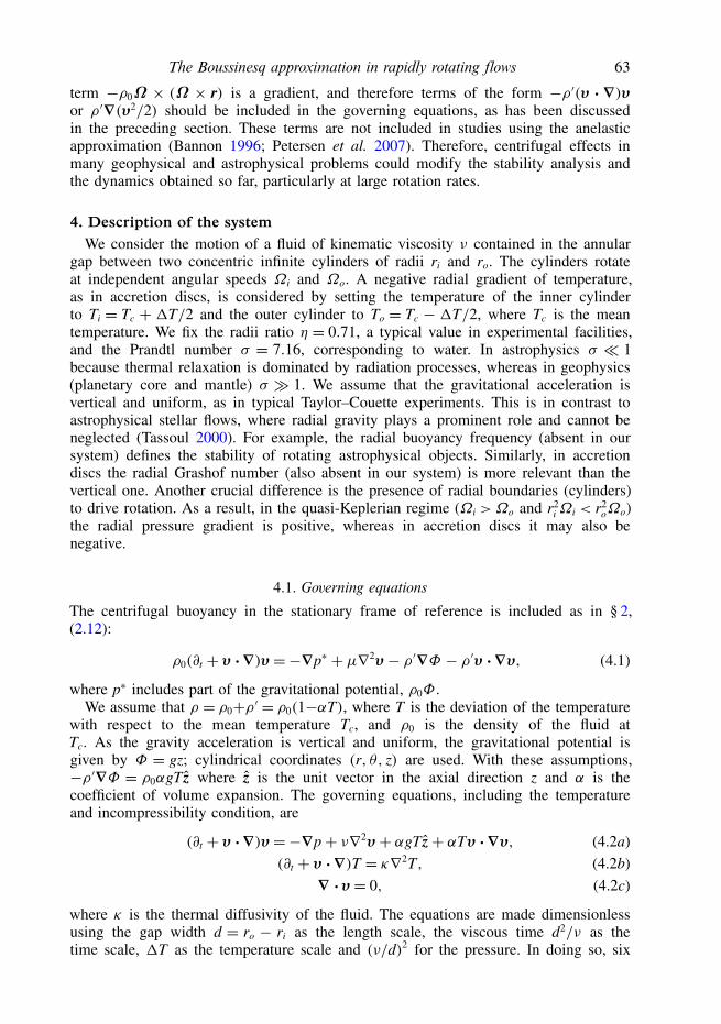
gap between two concentric infinite cylinders of radii ri and ro. The cylinders rotateat independent angular speeds Ωi and Ωo. A negative radial gradient of temperature,as in accretion discs, is considered by setting the temperature of the inner cylinderto Ti = Tc + 1T/2 and the outer cylinder to To = Tc − 1T/2, where Tc is the meantemperature. We fix the radii ratio η = 0.71, a typical value in experimental facilities,and the Prandtl number σ = 7.16, corresponding to water. In astrophysics σ 1because thermal relaxation is dominated by radiation processes, whereas in geophysics(planetary core and mantle) σ 1. We assume that the gravitational acceleration isvertical and uniform, as in typical Taylor–Couette experiments. This is in contrast toastrophysical stellar flows, where radial gravity plays a prominent role and cannot beneglected (Tassoul 2000). For example, the radial buoyancy frequency (absent in oursystem) defines the stability of rotating astrophysical objects. Similarly, in accretiondiscs the radial Grashof number (also absent in our system) is more relevant than thevertical one. Another crucial difference is the presence of radial boundaries (cylinders)to drive rotation. As a result, in the quasi-Keplerian regime (Ωi >Ωo and r2

iΩi < r2oΩo)

the radial pressure gradient is positive, whereas in accretion discs it may also benegative.

4.1. Governing equations

The centrifugal buoyancy in the stationary frame of reference is included as in § 2,(2.12):

ρ0(∂t + v ·∇)v=−∇p∗ + µ∇2v− ρ ′∇Φ − ρ ′v ·∇v, (4.1)

where p∗ includes part of the gravitational potential, ρ0Φ.We assume that ρ = ρ0+ρ ′ = ρ0(1−αT), where T is the deviation of the temperature

with respect to the mean temperature Tc, and ρ0 is the density of the fluid atTc. As the gravity acceleration is vertical and uniform, the gravitational potential isgiven by Φ = gz; cylindrical coordinates (r, θ, z) are used. With these assumptions,−ρ ′∇Φ = ρ0αgT z where z is the unit vector in the axial direction z and α is thecoefficient of volume expansion. The governing equations, including the temperatureand incompressibility condition, are

(∂t + v ·∇)v=−∇p+ ν∇2v+ αgT z+ αTv ·∇v, (4.2a)(∂t + v ·∇)T = κ∇2T, (4.2b)

∇ ·v= 0, (4.2c)

where κ is the thermal diffusivity of the fluid. The equations are made dimensionlessusing the gap width d = ro − ri as the length scale, the viscous time d2/ν as thetime scale, 1T as the temperature scale and (ν/d)2 for the pressure. In doing so, six


independent dimensionless numbers appear:

Grashof number G= αg1Td3/ν2, (4.3a)Relative density variation ε = α1T =1ρ/ρ0, (4.3b)

Prandtl number σ = ν/κ, (4.3c)Radius ratio η = ri/ro, (4.3d)

Inner Reynolds number Rei =Ωirid/ν, (4.3e)Outer Reynolds number Reo =Ωorod/ν. (4.3f )

where 1ρ is the density variation associated with a temperature change of 1T . In thissystem the Froude number is not particularly useful because we have two differentrotation rates, Ωi and Ωo, so the Froude number definition is not unique.

From now on, only dimensionless variables and parameters will be used. Thedimensionless governing equations are

(∂t + v ·∇)v=−∇p+∇2v+ GT z+ εTv ·∇v, (4.4a)(∂t + v ·∇)T = σ−1∇2T, (4.4b)

∇ ·v= 0, (4.4c)

The only change needed to recover the traditional Boussinesq approximation is toreplace the centrifugal term εTv · ∇v in (4.4a) by −εΩ2Trr, where r is the unit vectorin the radial direction r.

4.2. Base flowAn analytical solution for the base flow can be found by assuming only radialdependence for the variables of the problem. We also use the zero axial mass fluxcondition to fix the axial pressure gradient, i.e.∫ ro

ri

rwb(r) dr = 0. (4.5)

The resulting steady base flow is given by

ub(r)= 0 (4.6a)

vb(r)= Ar + B

r(4.6b)

wb(r)= G

(C(r2 − r2

i )+(

C(r2o − r2

i )+14(r2

o − r2)

)ln(r/ri)

ln η

)(4.6c)

Tb(r)= 12+ ln(r/ri)

ln η(4.6d)

p(r, z)= po + G

(4C + 1

2− 1

ln η

)z+

∫ r

ri

(1− εTb(r))v2b(r)

dr

r, (4.6e)

where (u, v,w) are the radial, azimuthal and axial components of the velocity field,and cylindrical coordinates (r, θ, z) are being used. Here vb is the azimuthal velocityfor the classical Taylor–Couette problem (Chandrasekhar 1961), whereas wb and Tb

correspond to convection in a conductive regime and appeared for the first time inChoi & Korpela (1980). The pressure varies linearly with the axial coordinate z, butthe pressure gradient depends only on r, and therefore it is periodic in the axialdirection. This axial pressure gradient mimics the presence of distant endwalls in any


real situation, by enforcing the zero mass flux constraint (4.5). It is possible to givean explicit closed expression for p by integrating (4.6e), but it is quite involved and itdoes not appear in the problem solution. The expressions for the parameters A, B andC are

A= Reo − ηRei

1+ η , B= η Rei − ηReo

(1− η)(1− η2), (4.7)

C =− 4 ln η + (1− η2)(3− η2)

16(1− η2)((1+ η2) ln η + 1− η2), (4.8)

where (4.7) define the pure rotational flow in the azimuthal coordinate and C givesthe axial component of the velocity field. The non-dimensional radii of the cylindricalwalls are given by ri = η/(1 − η), ro = 1/(1 − η). Note that the presence of the newcentrifugal buoyancy term, proportional to ε, does not modify the base flow’s velocityfield, but only its pressure.

4.3. Linearized equationsWe perturb the base flow with infinitesimal perturbations which vary periodically inthe axial and azimuthal directions,

v(r, θ, z, t)= vb(r)+ ei(nθ+kz)+λtu(r), (4.9a)

T(r, θ, z, t)= Tb(r)+ ei(nθ+kz)+λtT ′(r), (4.9b)

where vb = (0, vb,wb) and Tb(r) correspond to the base flow equation (4.6);u(r)= (ur, uθ , uz) and T ′(r) are the velocity and temperature perturbations, respectively.The boundary conditions for both u and T ′ are homogeneous: u(ri) = u(ro) = T ′(ri) =T ′(ro) = 0. The axial wavenumber k and the azimuthal mode number n define theshape of the disturbance. The parameter λ is complex. Its real part λr is theperturbation’s growth rate, which is zero at critical values, and its imaginary partλi is the oscillation frequency of the perturbation.

Using the decomposition (4.9) in the equations (4.4) and neglecting high-orderterms, we obtain an eigenvalue problem, with eigenvalue λ. It reads

λur = 1r

∂

∂r

(r∂ur

∂r

)− ur

[n2 + 1

r2+ k2 + i

(nvb

r+ kwb

)(1− εTb)

]+ 2vb

r(1− εTb)uθ − 2in

r2uθ − εv

2b

rT ′, (4.10a)

λuθ = 1r

∂

∂r

(r∂uθ∂r

)− uθ

[n2 + 1

r2+ k2 + i

(nvb

r+ kwb

)(1− εTb)

]−(∂vb

∂r+ vb

r

)(1− εTb)ur + 2in

r2ur, (4.10b)

λuz = 1r

∂

∂r

(r∂uz

∂r

)− uz

[n2

r2+ k2 + i

(nvb

r+ kwb

)(1− εTb)

]+ ∂wb

∂r(εTb − 1)ur + GT ′, (4.10c)

λT ′ = 1σ r

∂

∂r

(r∂T ′

∂r

)− T ′

[1σ

(n2

r2+ k2

)+ i(nvb

r+ kwb

)]− ∂Tb

∂rur. (4.10d)


Note that here the continuity equations and pressure terms are omitted becausethe Petrov–Galerkin method chosen to solve the resulting system of equationsautomatically satisfies the continuity equation and eliminates the pressure by usinga proper projection (see the next section).

From (4.10) the equations for the traditional Boussinesq approximation can beeasily obtained by setting ε = 0 in all terms except for −ε(v2

b/r)T′. The traditional

approximation incorporates only one rotating frame of reference for the system; theexpression (4.6b) for the base flow azimuthal velocity vb(r)= Ar + B/r has two terms,Ar corresponding to solid-body rotation and B/r corresponding to shear. It is natural toidentify A as the frequency of the rotating frame of reference, Ωr. In fact, if we takeΩi =Ωo =Ω , the Couette flow profile is

vb(r)= Ar + B

r= Ωor2

o −Ωir2i

r2o − r2

i

r + (Ωi −Ωo)(riro)2

r2o − r2

i

1r=Ωr =Ωrr, (4.11)

and we recover the linearized version of the centrifugal term considered in thetraditional approach, −εΩ2T ′rr. In the general case with Ωi 6= Ωo the traditionalBoussinesq approximation is defined in the frame of reference rotating with Ωr = A.This approximation takes only into account the centrifugal buoyancy acting in theradial direction, which is obviously its main contribution. However, as we will seein § 6, for high rotation rates other terms acting both in the radial and azimuthaldirections become important and change the behaviour of the system. Part of thediscrepancy stems from the fact that the effect of differential rotation is entirelyneglected in the traditional approximation.

5. Numerical methodIn order to solve numerically the eigenvalue problem described in the previous

section, a spatial discretization of the domain must be made. This is accomplished byprojecting the equations (4.10) onto a basis carefully chosen to simplify the process,

V3 = v ∈ (L2(ri, ro))3 |∇ ·v= 0,v(ri)= v(ro)= 0, (5.1)

where (L2(ri, ro))3 is the Hilbert space of square integrable vectorial functions defined

on the interval (ri, ro), with the inner product

〈v,u〉 =∫ ro

ri

v∗ ·ur dr, (5.2)

where ∗ denotes the complex conjugate. For any v ∈ V3 and any function p, using theincompressibility condition, the boundary conditions and integrating by parts,

〈v,∇p〉 =∫ ro

ri

(v∗ ·∇p)r dr =∫ ro

ri

rv∗r ∂rp dr = rpv∗r |rori−∫ ro

ri

p∂r(rv∗r ) dr = 0. (5.3)

This consideration allows us to eliminate the pressure from the equations as we projectthem onto the basis (Canuto et al. 2007). Moreover, the continuity equation is satisfiedby definition of the space V3. For the temperature perturbation the appropriate space is

V1 = f ∈L2(ri, ro) | f (ri)= f (ro)= 0. (5.4)


We expand the variables of the problem as follows

X =[u(r)T ′(r)

]=∑

j

ajXj Xj ∈ V3 × V1, (5.5)

and projecting (4.10) onto V3 × V1, we arrive at a linear system of equations for thecoefficients aj.

The solution of the system is performed by means of a Petrov–Galerkin scheme,where the basis used in the expansion is different from that used in the projection.The bases are composed of functions built on Chebyshev polynomials satisfying theboundary conditions. A detailed description of the method as well as the basis andfunctions used for the velocity field can be found in Meseguer & Marques (2000)and Meseguer et al. (2007), respectively. The basis functions for the temperature (lastcomponent of Xj in (5.5)), and for the projection (with ˜ ) are

hj(r)= (1− y2)Tj−1(y), hj(r)= r2(1− y2)Tj−1(y), (5.6)

where y = 2(r − ri) − 1 and Tj are the Chebyshev polynomials. As a result of thisprocess, we obtain a generalized eigenvalue system of the form

λM1x=M2x, (5.7)

where x is a vector containing the complex spectral coefficients (aj) and the matricesM1 and M2 depend on the parameters of the problem, the axial wavenumber k andthe azimuthal mode n. This system is solved by using LAPACK. The numerical codewritten to perform this work implements the described method and analyses a rangeof k, n and G provided by the user for a fixed Re number, searching for the criticalvalues (Re λ= λr = 0). Up to M = 200 radial modes have been used in order to ensurethe spectral convergence when high Re numbers are considered. The code has beentested by computing critical values for several cases in McFadden et al. (1984) and Ali& Weidman (1990), obtaining an excellent agreement with their results, as shown intable 1: the critical values computed coincide up to the last digit shown with those inthe mentioned references. In both cases the outer cylinder is at rest (Reo = 0).

6. Stability of differentially heated fluid between corotating cylindersIn this section we present a detailed comparison of the linear stability of the system

using the traditional Boussinesq approximation and the new approximation (4.10). Weconsider three different cases, all with η = 0.71 and σ = 7.16. In the first one thecylinders are rotating at same angular speed, corresponding to fluid rotating as a solidbody. In the second and third cases the stability of a differentially rotating fluid isconsidered in the presence of weak and strong (quasi-Keplerian) shear.

6.1. Cylinders rotating at the same angular speedIn this case a rotating frame of reference is readily identified and the shear term B/rin the base flow azimuthal velocity (4.6b) is zero, whereas the term A corresponds tothe angular velocity of the cylinders. Figure 1 shows the critical values of G as therotation speed, indicated here by the inner cylinder Reynolds number Rei, is increased.In the case of stationary cylinders instability sets in at G = 8087.42, with kc = −2.74and n = 0. The emerging pattern is characterized by pairs of counter-rotating toroidalrolls, that unlike Taylor vortices have a non-zero phase velocity that causes a slowdrift of the cellular pattern upward. Extensive information about natural convection


Parameters Critical values

η σ Ta Gc kc nc λi c= |λi|/kc

(a) 0.99 0.71 0 8038.0 2.80 0 0.254240.60 0.71 0 8512.4 2.75 0 13.398990.60 3.5 0 8347.5 2.75 0 12.977440.99 3.5 0 7857.1 2.75 0 0.24673

(b) 0.6 4.35 2591.0 50.0 3.15 0 −0.502940.6 4.35 380.3 700.0 1.88 −3 18.668890.6 15 111.1 280.0 1.68 −2 6.589160.6 15 26.88 700.0 0.77 −4 7.19973

TABLE 1. Code testing. The cases computed correspond to parameter values in (a)McFadden et al. (1984, table 1) and (b) Ali & Weidman (1990, table 1, p. 67). HereTa = 2(1 − η)Rei/(1 + η) is the Taylor number, λi = Im[λ] is the imaginary part of thecritical eigenvalue, for which Re[λ] = 0 and c is the dimensionless axial wave speed. Thesign of nc in our computation is opposite to that of Ali & Weidman (1990) because of thedefinition of the normal Fourier modes in (4.9).

instabilities can be found in the literature: Choi & Korpela (1980) and McFaddenet al. (1984) for infinite geometries, and de Vahl Davis & Thomas (1969) and Lee,Korpela & Horn (1982) for finite geometries. Without rotation, traditional (dashedline) and new (solid line) approximations yield identical results to the case wherecentrifugal buoyancy is neglected (dashed-dotted line). For slow rotation the effectof the centrifugal buoyancy is negligible, and nearly the same critical values areobtained in each case (see the inset in figure 1). As rotation is increased, the flowis strongly stabilized by centrifugal buoyancy. Note that if this is neglected, the onsetof instability asymptotically approaches Gc = 172.50 and is qualitatively wrong. Thepresence of the centrifugal term in any of the ways considered here, entirely modifiesthe stability of the problem and consequently is an essential element to study theseflows. No differences between the two approximations in the linear behaviour of thesystem are observed up to Rei ∼ 5 × 105, where the two curves start to depart fromeach other. Up to this point and after a small initial region where several azimuthalmodes up to n = 6 are involved, the base flow loses stability to an azimuthal moden = 1 with small axial wavenumber k ∼ 10−3. The shape of the critical modes alongthe stability curve is illustrated in figure 2, showing contours of constant temperaturein a horizontal cross-section. The three states correspond to the circles in figure 1and depict the transition between the lower and intermediate branches as we considerthe new approximation. As we proceed forward along the critical curve the cold fluidprogressively penetrates into the warm fluid and vice versa. The same behaviour isobserved when the traditional approximation is used, nevertheless the values of Rei

and Gc required are larger.As Rei increases beyond 5 × 105 the new terms in our approximation start

becoming important and lead to different behaviour in the linear stability of thesystem. An analysis of the magnitude of each term in our approximation revealsthat the differences observed in figure 1 at high Rei are due to terms involving theproduct vbuθ , implying the existence of an important centrifugal force acting in theazimuthal direction as high rotational speeds are reached. This provides evidencethat the traditional formulation, including only the main (radial) contribution ofcentrifugal buoyancy, is a very good approximation if slow rotation is involved but


Traditional approximationNew approximationWithout centrifugal term

0

2

4

6

8

10

2 4 6 8 10

102

102100

104

104

106

106

FIGURE 1. (Colour online) Critical Grashof number Gc as a function of the inner-cylinderReynolds number Rei for fluid rotating as a solid body. The solid line is the linear stabilitycurve using the new approximation for the centrifugal buoyancy proposed in this paper, thedashed corresponds to the traditional Boussinesq approach, whereas the dotted-dashed line isthe case without centrifugal buoyancy, which can only be distinguished from the horizontalaxis in the inset (log–log axes). Different symbols indicate the two distinct mechanismsof instability. Up and down triangles represent the critical points due to the mechanism atmoderate Rei for the new and traditional approximations respectively, whereas squares anddiamonds correspond to the mechanism at large Rei.

(a) (b) (c)

FIGURE 2. (Colour online) Contours of the temperature disturbance T ′ at a z-constantsection corresponding to the points marked as circles (shown in blue online) in figure 1:(a) Rei = 5 × 105, Gc = 21 206.53; (b) Rei = 5.7 × 105, Gc = 33 768.37; (c) Rei = 5.2 × 105,Gc = 79 670.16. There are 10 positive (dark grey; red in the online version) and 10 negative(light grey; yellow in the online version) linearly spaced contours. In all cases the criticalazimuthal mode is n= 1 and k = O(10−3).

other contributions may not be neglected in rapidly rotating fluids. Once the criticalvalues given by both approximations differ, we can identify two interesting regionsin parameter space. For Rei ∈ [5 × 105, 7.7 × 105] the traditional Boussinesq approach


0

1

2

3

2 4 6 80 10 2 4 6 80 10

–0.6

0

0 1000 2000

New aproximationTraditional approximation

–1

4

–40

–20

0

20

40

60

80

100

0

50

100

50 100

(a) (b)

FIGURE 3. (Colour online) (a) Critical axial wavenumber kc and (b) spiral angle of themodes arctan(kc/n) as a function of Rei for the curves in figure 1. The inset is a close up atlow Rei where the first mechanism stops being dominant and is superseded by spiral modeswith angle far from 90, indeed 0, corresponding to n= 0, at Rei = 0.

yields larger critical G than our approximation, whereas for Rei > 7.7 × 105 the upperbranch of the new approximation yields much lower critical values. Moreover, thedifferences keep increasing as Rei grows.

The analysis performed reveals the existence of two mechanisms of instabilityassociated with the lower-intermediate and upper branches in figure 1. Differentsymbols are used to represent the critical values corresponding to each mechanismin each problem. The differences between them are illustrated in figure 3, showingthe evolution of the critical axial wavenumber kc and the angle of the spiral modesarctan(kc/n) versus Rei. Two regions with distinct characteristics are well defined. Thefirst mechanism of instability has already been presented (see figure 2). Low azimuthalwavenumbers, primarily n= 1, and very small axial wavenumbers characterize it. Thiscorresponds to quasi two-dimensional modes and can be readily seen in figure 3(b),showing that the angle of the spiral modes remains constant at ∼90. The insetshows the small initial region where the spiral angle increases progressively untilit reaches a vertical position. The second mechanism is characterized by n > 80and kc ∼ O(1), also corresponding to quasi-two-dimensional modes (see figure 3b).Another common feature between the two types of instabilities is that the rotationalfrequency coincides with the angular velocity of the container in both mechanisms andboth approximations. This is in agreement with Maretzke, Hof & Avila (2013), whohave analytically proven that two-dimensional modes with k = 0 always rotate at speedA (4.6b) in Taylor–Couette flows without heating. An interesting distinct feature of thesecond instability mechanism is localization near the inner cylinder. An example ofthese wall convection modes is shown in figure 4; the critical disturbances are clearlydifferent in the traditional and in the new Boussinesq approximations.

6.2. Differentially rotating cylindersThe traditional approximation for the centrifugal buoyancy neglects the part of thebase flow containing shear, i.e. the B/r term in (4.6b). To quantify the influenceof including shear in the centrifugal terms, we perform the same analysis as inthe previous section but for differentially rotating cylinders. The amount of shearintroduced is characterized by the ratio of angular velocities β =Ωi/Ωo; the further βis from one, the stronger is the shear effect considered.


(a) (b)

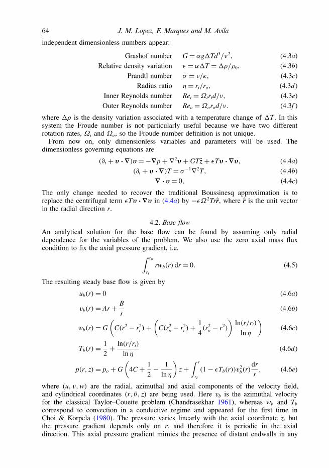
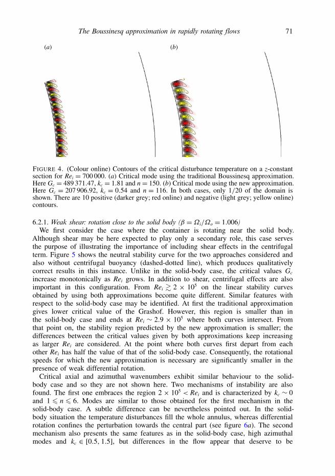
FIGURE 4. (Colour online) Contours of the critical disturbance temperature on a z-constantsection for Rei = 700 000. (a) Critical mode using the traditional Boussinesq approximation.Here Gc = 489 371.47, kc = 1.81 and n= 150. (b) Critical mode using the new approximation.Here Gc = 207 906.92, kc = 0.54 and n = 116. In both cases, only 1/20 of the domain isshown. There are 10 positive (darker grey; red online) and negative (light grey; yellow online)contours.

6.2.1. Weak shear: rotation close to the solid body (β =Ωi/Ωo = 1.006)We first consider the case where the container is rotating near the solid body.

Although shear may be here expected to play only a secondary role, this case servesthe purpose of illustrating the importance of including shear effects in the centrifugalterm. Figure 5 shows the neutral stability curve for the two approaches considered andalso without centrifugal buoyancy (dashed-dotted line), which produces qualitativelycorrect results in this instance. Unlike in the solid-body case, the critical values Gc

increase monotonically as Rei grows. In addition to shear, centrifugal effects are alsoimportant in this configuration. From Rei & 2 × 105 on the linear stability curvesobtained by using both approximations become quite different. Similar features withrespect to the solid-body case may be identified. At first the traditional approximationgives lower critical value of the Grashof. However, this region is smaller than inthe solid-body case and ends at Rei ∼ 2.9 × 105 where both curves intersect. Fromthat point on, the stability region predicted by the new approximation is smaller; thedifferences between the critical values given by both approximations keep increasingas larger Rei are considered. At the point where both curves first depart from eachother Rei has half the value of that of the solid-body case. Consequently, the rotationalspeeds for which the new approximation is necessary are significantly smaller in thepresence of weak differential rotation.

Critical axial and azimuthal wavenumbers exhibit similar behaviour to the solid-body case and so they are not shown here. Two mechanisms of instability are alsofound. The first one embraces the region 2 × 105 < Rei and is characterized by kc ∼ 0and 1 6 n 6 6. Modes are similar to those obtained for the first mechanism in thesolid-body case. A subtle difference can be nevertheless pointed out. In the solid-body situation the temperature disturbances fill the whole annulus, whereas differentialrotation confines the perturbation towards the central part (see figure 6a). The secondmechanism also presents the same features as in the solid-body case, high azimuthalmodes and kc ∈ [0.5, 1.5], but differences in the flow appear that deserve to be


2

4

6

0

8

2 4 6 8 10

New approximationTraditional approximationWithout centrifugal term

FIGURE 5. (Colour online) Critical Grashof number Gc as function of the inner-cylinderReynolds number Rei for rotation near the solid body (β = 1.006). Different symbols refer totwo distinct instability mechanisms as in figure 1.

(a) (b) (c)

FIGURE 6. (Colour online) Contours of the critical disturbance temperature on a z-constantsection: (a) n= 1, Rei = 178 125, Gc = 92 987.56. (b,c) Comparison of the traditional (b) andnew (c) approximation at Rei = 285 000 (near the crossover point in figure 5) showing 1/20of the annulus: (b) Gc = 154 864.79, kc = 0.24 and n = 30; (c) Gc = 156 547.54, kc = 0.39and n = 75. There are 10 positive (dark grey; red online) and negative (light grey; yellowonline) linearly spaced contours.

highlighted. In the traditional approximation the dominant wall modes are locatedat the inner cylinder, as occurs in the solid-body case (figure 6b). In contrast, usingthe new approximation changes the location of the dominant wall modes to the outercylinder (figure 6c). In view of these results we can say that considering shear effectsin the centrifugal term of the Navier–Stokes equations may be extremely important:not only regarding the linear stability boundary but also the shape and location of thecritical modes.


6.2.2. Strong shear: quasi-Keplerian rotation (β =Ωi/Ωo = 1.58)If 1/η > β > 1 the angular velocity decreases outward but the angular momentum

increases. These flows, known as quasi-Keplerian flows, are used as models toinvestigate the dynamics and stability of astrophysical accretion discs. Here wechoose a typical value β = 1.58 and as in the previous sections consider a negativetemperature gradient in the radial direction, as expected in accretion discs. Figure 7shows the neutral stability curve for the two approximations considered, as well asentirely neglecting centrifugal effects (ε = 0). The three curves are almost straightlines, that completely overlap in a plot (Gc,Rei). In order to see the small differencesthat appear at large Rei, we have plotted in this case Gc/Rei versus Rei. Shear is thecompletely dominant mechanism in this regime, but small differences can be observedfor Rei & 2 × 105, that are enhanced in the inset. Surprisingly, shear has a very strongstabilizing effect in this problem: without shear the critical Grashof number is 10 timessmaller at Rei = 106 than in the quasi-Keplerian case.

Depending on the Reynolds number two mechanisms of instability are again found.The first mechanism exhibits a similar flow structure to that observed in the previouscase. It also occurs at low Rei and is localized in the central part of the annulus dueto the action of differential rotation. Figure 8(a) shows the contours of the disturbancetemperature in a horizontal plane. In contrast to what happens in the weak shearsituation, these modes present a clear three-dimensional structure with kc ∼ −1. Smallazimuthal wavenumbers are involved in this mechanism, ranging from n = 1 to n = 6.More remarkable differences are found when analysing the second mechanism. Highazimuthal modes n ∼ 50 arise as this mechanism becomes dominant, but unlike thesolid-body and weak-shear situations, the azimuthal mode number decreases as Rei

increases. The same behaviour is observed in the axial wavenumber, so that the spiralangle quickly converges to 90 as observed in the previous sections. Figure 8(b) showsthat the instability is characterized by convection wall modes localized at the outercylinder, as in the case of weak shear using the new approximation. Nevertheless, inquasi-Keplerian flows the dominant modes are always localized at the outer cylinderregardless of how centrifugal terms enter the equations.

7. Summary and discussionWe have identified weaknesses in how the Boussinesq formulation is typically used

to account for centrifugal buoyancy in the Navier–Stokes equations. In particular,the traditional approximation (including only the term ρ ′Ω2) neglects the effectsassociated with differential rotation or strong internal vorticity. This has motivatedus to develop a new consistent Boussinesq-type approximation correcting this problem.It consists of keeping the density variations in the advection term of the Navier–Stokesequations and, thus, it is very easy to implement in an existent solver. The newapproximation allows accurate treatment of situations with differential rotation or whenstrong vortices appear in the interior of the domain, which may cause importantcentrifugal effects even in flows without global rotation. The latter may be especiallyrelevant in simulations at high Rayleigh numbers (as e.g. in the quest for the ‘ultimateregime’; (Ahlers, Grossmann & Lohse 2009)). Thus, we argue that our formulationfor the centrifugal terms should be always implemented whenever the Boussinesqapproximation is used.

The relevance of the new approximation has been illustrated with a linear stabilityanalysis of a Taylor–Couette system subjected to a negative radial gradient oftemperature. Three different cases have been studied. First, we have considered the


3.2

3.6

4.0

0 2 4 6 8 10

3.05

3.06

3.07

3.08

9.0 9.1 9.2

New approximationTraditional approximationWithout centrifugal term

FIGURE 7. (Colour online) Critical ratio Gc/Rei as function of inner cylinder Reynoldsnumber Rei for quasi-Keplerian rotation (β = 1.58). The three curves differ only by ∼1 % andhence are only distinguishable in the inset.

(a) (b)

FIGURE 8. (Colour online) Contours of the critical disturbance temperature on a z-constant section: (a) Rei = 11 681.03 with Gc = 4.1268 × 104, kc = −1.05 and n = 1; (b)Rei = 584 051.72 with Gc = 1.8511 × 104, kc = 8.21 and n = 38. Ten positive (dark grey;red online) and negative contours (light grey; yellow online) are displayed. Only 1/20 of thedomain is shown in (b).

container rotating as a solid body, i.e. without differential rotation. We note that ifcentrifugal buoyancy is entirely neglected, the results are even qualitatively wrong.For both traditional and new approximations the critical values obtained agree up toRei ∼ 5.5 × 105, beyond which discrepancies become significant. Beyond this pointthe conductive base flow loses stability to quasi two-dimensional wall modes (aligned


with the axis of rotation, as expected from the Taylor–Proudman theorem) localizedat the inner cylinder. Note that the large discrepancy in critical Grashof numbersobserved at Rei ∈ [5× 105, 106] between both approximations makes it possible to testthem against laboratory experiments. For example, in the experiments from Paoletti &Lathrop (2011) and Avila & Hof (2013), which allow for radial temperature gradients,Re = 106 can be reached, and the required Grashof numbers 5 × 105 can be obtainedwith temperature differences about half a degree Kelvin.

We have also considered the case in which the cylinders rotate at different angularspeeds, thus introducing shear. For weak differential rotation, shear and centrifugalbuoyancy effects compete and the critical values obtained with both approximationsdiffer from each other at lower Rei ∼ 2 × 105. Moreover, the new approximation givesrise to wall modes located on the outer cylinder, whereas the traditional approachyields wall modes on the inner cylinder, as in the solid-body case. In quasi-Keplerianflows, shear is so dominant that centrifugal terms may be entirely neglected inthe linear stability analysis (discrepancies in Gc are below 1 % regardless of howcentrifugal terms enter the equations, if at all). Here the critical modes are alwayslocalized at the outer cylinder. Note that such wall modes, similar to those identifiedby Klahr, Henning & Kley (1999), are not relevant to the accretion-disc problem,in which there are no solid radial boundaries. Furthermore, it is worth noting thattesting our differential rotation results in the laboratory is very difficult because ofaxial endwall effects. The large Re involved will necessarily trigger instabilities andtransition to turbulence because of the nearly discontinuous angular velocity profile atthe junction between axial endwalls and cylinders (Avila 2012).

Although it may be tempting to suggest that laminar quasi-Keplerian flows are stablefor weak stratification in the radial direction, our analysis has only axial gravity, andis linear and hence concerned with infinitesimal disturbances only. In more realisticmodels of accretion discs, nonlinear baroclinic instabilities have been found in similarregimes by Klahr & Bodenheimer (2003), and we expect that subcritical transition viafinite-amplitude disturbances may occur in the problem investigated here. This remainsa key question for incoming numerical and experimental investigations. In fact, evenin the classical (isothermal) Taylor–Couette problem this possibility remains open andcontroversial (see e.g. Balbus 2011).

AcknowledgementsThis work was supported by the Spanish Government grants FIS2009-08821 and

BES-2010-041542. Part of the work was done during J.M.L’s visit to the Instituteof Fluid Mechanics at the Friedrich-Alexander-Universitat Erlangen-Nurnberg, whosekind hospitality is warmly appreciated.

R E F E R E N C E S

AHLERS, G., GROSSMANN, S. & LOHSE, D. 2009 Heat transfer and large-scale dynamics inturbulent Rayleigh–Benard convection. Rev. Mod. Phys. 81 (2), 503–537.

ALI, M. E. & WEIDMAN, P. D. 1990 On the stability of circular Couette-flow with radial heating.J. Fluid Mech. 220, 53–84.

ARFKEN, G. B. & WEBER, H. J. 2005 Mathematical Methods for Physicists, 6th edn. Academic.AVILA, M. 2012 Stability and angular-momentum transport of fluid flows between corotating

cylinders. Phys. Rev. Lett. 108, 124501.AVILA, K. & HOF, B. 2013 High-precision Taylor–Couette experiment to study subcritical transitions

and the role of boundary conditions and size effects. Rev. Sci. Instrum. 84, 065106.


BALBUS, S. A. 2003 Enhanced angular momentum transport in accretion disks. Annu. Rev. Astron.Astrophys. 41 (1), 555–597.

BALBUS, S. A. 2011 Fluid dynamics: a turbulent matter. Nature 470 (7335), 475–476.BANNON, P. R. 1996 On the anelastic approximation for a compressible atmosphere. J. Atmos. Sci.

53 (23), 3618–3628.BARCILON, V. & PEDLOSKY, J. 1967 On the steady motions produced by a stable stratification in a

rapidly rotating fluid. J. Fluid Mech. 29, 673–690.BATCHELOR, G. K. 1967 An Introduction to Fluid Mechanics. Cambridge University Press.BOUSSINESQ, J. 1903 Theorie Analytique de la Chaleur, vol. II, Gauthier-Villars.BRUMMELL, N., HART, J. E. & LOPEZ, J. M. 2000 On the flow induced by centrifugal buoyancy

in a differentially-heated rotating cylinder. Theor. Comput. Fluid Dyn. 14, 39–54.CANUTO, C., QUARTERONI, A., HUSSAINI, M. Y. & ZANG, T. A. 2007 Spectral Methods.

Evolution to Complex Geometries and Applications to Fluid Dynamics. Springer.CHANDRASEKHAR, S. 1961 Hydrodynamic and Hydromagnetic Stability. Oxford University Press.CHOI, I. G. & KORPELA, S. A. 1980 Stability of the conduction regime of natural convection in a

tall vertical annulus. J. Fluid Mech. 99, 725–738.ELPERIN, T., KLEEORIN, N. & ROGACHEVSKII, I. 1998 Dynamics of particles advected by fast

rotating turbulent fluid flow: fluctuations and large-scale structures. Phys. Rev. Lett. 81,2898–2901.

HART, J. E. 2000 On the influence of centrifugal buoyancy on rotating convection. J. Fluid Mech.403, 133–151.

HIDE, R. & FOWLIS, W. W. 1965 Thermal convection in a rotating annulus of liquid: effectof viscosity on the transition between axisymmetric and non-axisymmetric flow regimes.J. Atmos. Sci. 22, 541–558.

HOMSY, G. M. & HUDSON, J. L. 1969 Centrifugally driven thermal convection in a rotatingcylinder. J. Fluid Mech. 35, 33–52.

KLAHR, H. & BODENHEIMER, P. 2003 Turbulence in accretion disks: vorticity generation andangular momentum transport via the global baroclinic instability. Astrophys. J. 582 (2),869–892.

KLAHR, H. H., HENNING, TH. & KLEY, W. 1999 On the azimuthal structure of thermal convectionin circumstellar disks. Astrophys. J. 514 (1), 325–343.

LEE, Y., KORPELA, S. A. & HORN, R. N. 1982 Structure of multicellular natural convection in atall vertical annulus. In Proceedings of the 7th International Heat Transfer Conference,Munich, vol. 2, pp. 221–226.

LESUR, G. & PAPALOIZOU, J. C. B. 2010 The subcritical baroclinic instability in local accretiondisc models. Astron. Astrophys. 513, A60.

LOPEZ, J. M. & MARQUES, F. 2009 Centrifugal effects in rotating convection: nonlinear dynamics.J. Fluid Mech. 628, 269–297.

MARETZKE, S., HOF, B. & AVILA, M. 2013 Transient growth in linearly stable Taylor–Couetteflows. J. Fluid Mech. (submitted).

MARQUES, F., MERCADER, I., BATISTE, O. & LOPEZ, J. M. 2007 Centrifugal effects in rotatingconvection: axisymmetric states and 3d instabilities. J. Fluid Mech. 580, 303–318.

MCFADDEN, G. B., CORIELL, S. R., BOISVERT, R. F. & GLICKSMAN, M. E. 1984 Asymmetricinstabilities in buoyancy-driven flow in a tall vertical annulus. Phys. Fluids 27, 1359–1361.

MESEGUER, A., AVILA, M., MELLIBOVSKY, F. & MARQUES, F. 2007 Solenoidal spectralformulations for the computation of secondary flows in cylindrical and annular geometries.Eur. Phys. J. Special Topics 146, 249–259.

MESEGUER, A. & MARQUES, F. 2000 On the competition between centrifugal and shear instabilityin spiral Couette flow. J. Fluid Mech. 402, 33–56.

PAOLETTI, M. S. & LATHROP, D. P. 2011 Measurement of angular momentum transport inturbulent flow between independently rotating cylinders. Phys. Rev. Lett. 106, 024501.

PETERSEN, M., JULIEN, K. & STEWART, G. 2007 Baroclinic vorticity production in protoplanetarydisks. Astrophys. J. 658, 1236–1251.


RANDRIAMAMPIANINA, A., FRUH, W.-G., READ, P. L. & MAUBERT, P. 2006 Direct numericalsimulations of bifurcations in an air-filled rotating baroclinic annulus. J. Fluid Mech. 561,359–389.

REGEV, O. & UMURHAN, O. M. 2008 On the viability of the shearing box approximation fornumerical studies of mhd turbulence in accretion disks. Astron. Astrophys. 481 (1), 21–32.

TASSOUL, J. L. 2000 Stellar Rotation. Cambridge University Press.DE VAHL DAVIS, G. & THOMAS, R. W. 1969 Natural convection between concentric vertical

cylinders. Phys. Fluids Suppl. II. 198–207.

the boussinesq approximation in rapidly rotating ï¬‚ows

Documents