the boreal-summer intraseasonal oscillations simulated in...
TRANSCRIPT

2628 VOLUME 132M O N T H L Y W E A T H E R R E V I E W
q 2004 American Meteorological Society
The Boreal-Summer Intraseasonal Oscillations Simulated in a Hybrid CoupledAtmosphere–Ocean Model*
XIOUHUA FU AND BIN WANG
International Pacific Research Center, School of Ocean and Earth Science and Technology, University of Hawaii at Manoa,Honolulu, Hawaii
(Manuscript received 9 September 2003, in final form 15 May 2004)
ABSTRACT
The boreal-summer intraseasonal oscillation (BSISO) simulated by an atmosphere–ocean coupled model isvalidated with the long-term observations [Climate Prediction Center (CPC) Merged Analysis of Precipitation(CMAP) rainfall, ECMWF analysis, and Reynolds’ SST]. This validation focuses on the three-dimensional watervapor cycle associated with the BSISO and its interaction with underlying sea surface. The advantages of acoupled approach over stand-alone atmospheric approaches on the simulation of the BSISO are revealed throughan intercomparison between a coupled run and two atmosphere-only runs.
This coupled model produces a BSISO that mimics the one presented in the observations over the Asia–western Pacific region. The similarities with the observations include 1) the coherent spatiotemporal evolutionsof rainfall, surface winds, and SST associated with the BSISO; 2) the intensity and period (or speed) of thenorthward-propagating BSISO; and 3) the tropospheric moistening (or drying) and overturning circulations ofthe BSISO. However, the simulated tropospheric moisture fluctuations in the extreme phases (both wet and dry)are larger than those in the ECMWF analysis. The simulated sea surface cooling during the wet phase is weakerthan the observed cooling. Better representations of the interaction between convection and boundary layer inthe GCM and including salinity effects in the ocean model are expected to further improve the simulation ofthe BSISO.
The intercomparison between a coupled run and two atmospheric runs suggests that the air–sea coupled systemis the ultimate tool needed to realistically simulate the BSISO. Though the major characteristics of the BSISOare very likely determined by the internal atmospheric dynamics, the correct interaction between the internaldynamics and underlying sea surface can only be sustained by a coupled system. The atmosphere-only approach,when forced with high-frequency (e.g., daily) SST, introduces an erroneous boundary interference on the internaldynamics associated with the BSISO. The implications for the predictability of the BSISO are discussed.
1. Introduction
Intraseasonal oscillation (ISO) is an essential com-ponent of the Asia–western Pacific summer monsoonsystem (Krishnamurti 1985; Webster et al. 1998; Lau etal. 2000). The rainfall variance associated with the ISOexceeds considerably the variance associated with in-terannual fluctuations in the monsoon area (Waliser etal. 2003a). Regionally, these intraseasonal oscillationsstrongly regulate the onset (retreat) and active (break)spells of the Asian summer monsoon (e.g., Yasunari1979; Lau and Chan 1986; Kang et al. 1999; Senguptaet al. 2001; Wu et al. 2002; Fu et al. 2002). Through
* School of Ocean and Earth Science and Technology ContributionNumber 6429 and International Pacific Research Center ContributionNumber 282.
Corresponding author address: Dr. Xiouhua Fu, IPRC, SOEST,University of Hawaii at Manoa, 1680 East–West Road, POST Bldg.401, Honolulu, HI 96822.E-mail: [email protected]
teleconnection, the ISO that originates in the Asia–west-ern Pacific region modulates the subseasonal rainfallvariability in the extratropical region (Kawamura et al.1996), even over North America (Mo 2000). Better un-derstanding and simulation of the ISO are expected toextend our forecasting capability with a time advanceof about one month (Krishnamurti et al. 1992; Waliseret al. 2003b), which bridges the gap between weatherforecasting (;one week) and seasonal climate predic-tion (;a few months).
State-of-the-art atmospheric general circulation mod-els (GCMs) have shown some successes in simulatingthe intraseasonal oscillations (Slingo et al. 1996; Sper-ber et al. 1997). Many models are able to produce robusteastward-propagating Madden–Julian oscillations(MJOs; Madden and Julian 1971) gauged with plane-tary-scale upper-layer velocity potential variability.Most GCMs, however, cannot yet realistically simulatethe BSISO associated with the Asia–western Pacificsummer monsoon in terms of its intensity and propa-gation (Waliser et al. 2003a). All 10 GCMs participating

NOVEMBER 2004 2629F U A N D W A N G
in the Climate Variability and Predictability program(CLIVAR)/Asian–Australian monsoon intercomparisonproject (Kang et al. 2002) considerably underestimatethe intraseasonal variability near the equatorial IndianOcean, where the observed ISO has its largest amplitudeyear-round and a favorable region of amplification(Wang and Rui 1990). Though most of these GCMsproduce strong summer-mean Indian monsoon rainfall,the simulated northward-propagating intraseasonal os-cillations remain systematically weaker than the ob-served (Waliser et al. 2003a). This finding implies thatreasonable simulation of summer-mean Indian monsoonrainfall (with a dominant rainbelt around 158N) does notnecessarily yield a successful simulation of the boreal-summer ISO (BSISO) with its origin and an action cen-ter near the equatorial Indian Ocean and preferentialnortheastward propagation in the Asia–western Pacificregion (Yasunari 1979; Lau and Chan 1986; Wang andRui 1990).
Intraseasonal oscillation has its roots in internal at-mospheric dynamics (Chang 1977; Lau and Peng 1987;Wang 1988; Blade and Hartmann 1993; Hu and Randall1994; Neelin and Yu 1994; Raymond 2001, among oth-ers). This has been supported by the fact that an at-mosphere-only model is able to produce an oscillationsimilar to the MJO. On the other hand, Wang and Xie(1998) proposed that warm-pool air–sea coupling is ableto contribute to the growth and maintenance of an MJO-like mode. In fact, significant SST fluctuations associ-ated with the ISO in the tropical Indian and westernPacific Oceans have long been documented by Krish-namurti et al. (1988). With the data from the TropicalOcean Global Atmosphere Coupled Ocean–AtmosphereResponse Experiment (TOGA COARE; Webster andLukas 1992), Zhang (1996) also documented the co-herent relationships between MJO and underlying SSTfluctuations. These findings raised an important ques-tion: Are the intraseasonal SST fluctuations just passiveresponses to the atmospheric ISO or do the SST fluc-tuations significantly feed back to the ISO? A numberof modeling studies (Flatau et al. 1997; Waliser et al.1999; Hendon 2000; Kemball-Cook et al. 2002; Innessand Slingo 2003; Fu et al. 2003; Zheng et al. 2004;Rajendran et al. 2004) have attempted to address thisquestion. Almost all these studies (except Hendon 2000)have shown that air–sea interaction improves both theMJO in boreal winter and the BSISO in boreal summerin terms of their intensity, propagation, and seasonality.With a series of small-perturbation experiments, Fu andWang (2004) further showed that two different ISO so-lutions actually exist in the atmosphere–ocean coupledsystem and the forced atmosphere-only system, respec-tively. The solution in the coupled system is closer tothe observations. The exception of Hendon (2000) islargely attributed to the failure of the model to simulatea reasonable surface latent heat flux associated with themodel MJO. However, the exception of Hendon (2000)reminds us that air–sea coupling is not a panacea for
all the modeling problems of ISO, but may be viewedas a significant piece in the puzzle of realistically sim-ulating ISO. The representations of other pieces in thepuzzle, for example, cumulus parameterization (Tokiokaet al. 1988; Wang and Schlesinger 1999; Maloney andHartmann 2001), cloud–radiation interaction (Lee et al.2001), boundary layer processes (Wang 1988), and landsurface processes (Webster 1983), are also important inorder to advance our capability of simulating ISO withgeneral circulation models.
Using a hybrid coupled model (ECHAM4 GCM withthe Wang–Li–Fu intermediate ocean model), Fu et al.(2003) found that air–sea interaction significantly in-creases the intensity of the northward-propagating BSI-SO (NPISO) over the Indian sector. Forcing GCM withdaily mean SST produces a stronger NPISO comparedto that forced by monthly mean SST [Atmospheric Mod-el Intercomparison Project (AMIP)-type], but is still un-able to reproduce the NPISO intensity in the coupledmodel. The improved simulation of the NPISO in thishybrid-coupled model enables a further comprehensivemodel validation with the available observations. Weaddress the following three questions in this study: 1)In what aspects does this hybrid-coupled model yield areasonable simulation of the BSISO over the tropicalAsia–western Pacific region? 2) What are the obviousdiscrepancies with the available observations and thepossible causes? 3) To what degree can air–sea inter-action change the characteristics of the BSISO simulatedin the atmosphere-only model? We expect that this studywill lead us to better understand the major physical pro-cesses controlling the BSISO in the model and shedlight on the directions to further improve the model.
This validation focuses on the water vapor cycle ofthe BSISO (Myers and Waliser 2003) and its interactionwith underlying sea surface, in contrast to previous ap-proaches (Rui and Wang 1990; Hendon and Salby 1994;Slingo et al. 1996) that measured ISO with outgoinglongwave radiation (OLR) and two-layer dynamicalfields (e.g., velocity potential and zonal winds) at 850-and 200-hPa surfaces. The present approach is based onthe following assumptions: 1) an adequate representa-tion of tropospheric moistening associated with atmo-spheric convection is important to the initiation andmaintenance of ISO in GCMs (Tompkins 2001; Gra-bowski 2003) and 2) air–sea interaction plays an im-portant role on realistic simulation of ISO (Flatau et al.1997; Waliser et al. 1999).
This paper is structured as follows: The model anddata are introduced in section 2. The BSISO simulatedin the coupled model is validated with available obser-vations and compared to the simulations of atmosphere-only runs in the following two sections. In section 3,the comparisons are devoted to the horizontal patternsand temporal evolutions in the entire tropical Asia–west-ern Pacific region. Section 4 focuses on the NPISO inthe Indian Ocean sector. In the last section, we sum-

2630 VOLUME 132M O N T H L Y W E A T H E R R E V I E W
marize our results and discuss the model caveats andfuture studies.
2. Model and data
a. Model description and experimental designs
1) THE COUPLED MODEL
The atmospheric component of this coupled model isthe ECHAM4 GCM (Roeckner et al. 1996). Its hori-zontal resolution is about 3.758 in both longitude andlatitude (a T30 version), with 19 vertical levels extend-ing from the surface to 10 hPa. The mass flux schemeof Tiedtke (1989) is used to represent the deep, shallow,and midlevel convection. A CAPE closure scheme hasbeen implemented by Nordeng (1994) to replace theoriginal moisture-convergence closure. The ocean com-ponent of the coupled model is a 2.5-layer tropical up-per-ocean model with a horizontal resolution of 28 lon-gitude by 18 latitude. It was originally developed byWang et al. (1995) and improved by Fu and Wang (2001)(hereafter the WLF ocean model). The WLF ocean mod-el combines the mixed-layer thermodynamics of Gaspar(1988) and the upper-ocean dynamics of McCreary andYu (1992). The ocean model is able to simulate realisticannual cycles of SST, upper-ocean currents, and mixed-layer thickness in the tropical Pacific (Fu and Wang2001). The ECHAM4 GCM and WLF ocean model arecoupled in the tropical Indian and Pacific Oceans. Out-side these regions, the underlying SST is specified asthe climatological monthly mean SST averaged for 16yr (1979–94) from the boundary conditions of AMIPII experiments (Taylor et al. 2000). In the central-easternPacific (east of the date line), the model SST is relaxedtoward the observations in order to avoid excessivewestward extension of the Pacific cold tongue (Fu et al.2002). The atmospheric component exchanges infor-mation with the ocean component once per day. Theinitial atmospheric state is taken from the EuropeanCentre for Medium-Range Weather Forecasts(ECMWF) analysis on 1 January 1988. The initial oce-anic state is the January state after a 10-yr integrationof the stand-alone ocean model forced by observed cli-matological surface winds and heat fluxes. The coupledmodel is integrated for 16 yr, and the last 10 yr of therun are used in the analyses reported below. We referto this simulation as the ‘‘coupled run.’’
2) STAND-ALONE ATMOSPHERIC EXPERIMENTS
To assess the impacts of air–sea coupling and intra-seasonal SST fluctuations on the characteristics of theBSISO, two more sensitivity experiments are conductedwith the stand-alone ECHAM4 GCM. In the ‘‘mean’’experiment (AMIP-type), the climatological monthlymean SST from the coupled run is used to force themodel, and the initial conditions are the same as thosefor the coupled run. It is integrated for 16 yr, and the
output from the last 10 yr is used in the analyses. Inthe ‘‘daily’’ experiment, the SST forcing is daily meanSST from the last 10 yr of the coupled run, and theinitial conditions are unchanged.
b. Data and methods
The data used to validate the model are from theECMWF analysis (three-dimensional atmospheric fieldsand surface heat fluxes), Climate Prediction Center(CPC) Merged Analysis of Precipitation rainfall (Xieand Arkin 1997), and Reynolds’ SST (Reynolds andSmith 1994). All data cover the 10-yr period from 1991to 2000. The temporal resolutions for ECMWF analysis,CMAP, and Reynolds’ data are daily, pentad, and week-ly, respectively. In the following analyses, all data areaveraged or interpolated into pentad-mean data.
Because almost all the above datasets are not in situdata, they are actually proxies of the observations. Re-cently, two field campaigns, the Joint Air–Sea MonsoonInteraction Experiment (JASMINE; Webster et al. 2002)and the Bay of Bengal Monsoon Experiment (BOB-MEX; Bhat et al. 2001), have been carried out to in-vestigate the BSISO in the Indian Ocean. These obser-vations facilitate air–sea coupled process studies. How-ever, the limited numbers of the cases that occur duringthe campaign periods are too few to construct statisticalevolutions of the BSISO in the Asia–western Pacificsector. We are also aware that the rainfall and SST datafrom the Tropical Rainfall Measuring Mission (TRMM)Microwave Imager (TMI; Vecchi and Harrison 2002)are available for recent years. A preliminary comparisonbetween TMI data and the historical data (CMAP andReynolds) suggests that they are comparable during re-cent years in terms of the large-scale variations asso-ciated with the BSISO (figure not shown). Concerningthe short period of the available TMI data, we decidedto use those long-term proxies to surrogate the observedBSISO in this study. Because those proxy data usedhere are from different sources, the coherent evolutionsamong CMAP rainfall, Reynolds’ SST, and ECMWFanalysis of atmospheric variables and surface heat fluxessuggest the usefulness of these proxies. These proxydata will be referred as ‘‘observations’’ in the remainingtext.
In order to evaluate the simulated BSISO against theobservations as objectively as possible, several com-plementary methods for ISO analysis are applied. Thelag regression is used to document the spatiotemporalevolutions of precipitation, surface winds, and SST as-sociated with the BSISO. The wavenumber-frequencyanalysis (Hayashi 1982; Teng and Wang 2003; Fu et al.2003) is used to quantify the northward- and southward-propagating disturbances in the Indian sector. Tradi-tional composite analysis is also used to construct thevertical moisture (circulation) structures associated withthe NPISO. Except for the wavenumber-frequency anal-ysis (in which unfiltered rainfall data are used), all other

NOVEMBER 2004 2631F U A N D W A N G
analyses use the filtered 20–70-day variables (Rui andWang 1990).
3. The BSISO in the Asia–Pacific sector
a. Mean state and BSISO action centers
Figure 1 compares rainfall and zonal wind shear(850–200 hPa) from the observations, the mean run andthe coupled run in boreal summer [June–July–August–September (JJAS)]. Both model solutions (Figs. 1b and1c) capture the major rainfall areas and easterly shearsin the observations (Fig. 1a), but also have some sys-tematic errors. In the Indian sector, both runs reproducethe observed double rainbelts: one near the equator andthe other around 158N. The rainfall in the eastern Ara-bian Sea and Bay of Bengal is underestimated, thusyielding a weaker vertical shear in the Indian Ocean. Inspite of these biases, the simulations are relatively betterthan most GCMs participating in the AMIP monsoonintercomparison project (Gadgil and Sajani 1998) andthe CLIVAR/monsoon intercomparison project (Kanget al. 2002), in which only a few GCMs are able toproduce two convergence zones in the Indian sector.Many current GCMs tend to produce an excessivelystrong rainbelt near 158N (Kang et al. 2002) with theequatorial rainbelt significantly weakened or totally sup-pressed. The lack of active convection near the equa-torial Indian Ocean is probably one reason why the NPI-SOs in these GCMs are systematically weak (Waliseret al. 2003a). In the western North Pacific (WNP), thesimulated rainfall (Figs. 1b and 1c) is considerablysmaller than the observed (Fig. 1a), which is probablyassociated with the erroneously strong rainfall over thePhilippine Islands. The reason for this systematic errorof ECHAM4 GCM is unclear (Roeckner et al. 1996).The models (Figs. 1b and 1c) also tend to produce er-roneous double ITCZs in the western Pacific rather thana dominant northern one in the observations (Fig. 1a),probably a result of the cold bias in the coupled SST(Fig. 1c in Fu et al. 2003). The summer-mean rainfalland vertical shear in the daily run (forced by the dailymean SST of the coupled run) is similar to those in themean and coupled runs (Figs. 1b and 1c).
Figure 2 presents the standard deviation of tropicalintraseasonal rainfall in boreal summer over the Asia–western Pacific sector from the CMAP, the mean run,and the coupled run, respectively. In the observations(Fig. 2a), there are five active regions of the BSISO:the eastern Arabian Sea, Bay of Bengal, equatorial In-dian Ocean, South China Sea, and the WNP. In the at-mosphere-only run (Fig. 2b), the BSISO activities in theBay of Bengal, South China Sea, and eastern ArabianSea are considerably weaker than in the observations.Note that in the 10 GCMs evaluated by Waliser et al.(2003a), nearly all models missed the active ISO centerover the equatorial Indian Ocean, but ECHAM4 pro-duces significant intraseasonal variability there. It is
probably due to the large summer-mean convection inthis area (Roeckner et al. 1996; Fu et al. 2002). Com-pared to the mean run (Fig. 2b), the ISO variance issignificantly increased in the coupled run (Fig. 2c) overthe equatorial Indian Ocean, Bay of Bengal, South Chi-na Sea, and eastern Arabian Sea (the result of the dailyrun is stronger than the mean run, but weaker than thecoupled run; see Fig. 7 in this paper or Fig. 4 in Fu etal. 2003). Because the monthly mean SST of the coupledrun is used to force the atmospheric model in the meanrun, the resultant mean states in the two simulations(Figs. 1b and 1c) are very similar (see also Waliser etal. 1999). However, the differences in the ISO variabilitybetween the mean run (Fig. 2b) and the coupled run(Fig. 2c) are noticeable because of the impacts of air–sea coupling. In the coupled run the ISO intensity issignificantly enhanced over the equatorial Indian Ocean,Bay of Bengal, and South China Sea. As in the summer-mean states (Figs. 1b and 1c), an erroneously strongISO action center over the Philippine Islands is pro-duced in both the coupled run and the atmosphere-onlyrun, which may be responsible for the weak ISO in theWNP (Figs. 2b and 2c).
b. Coherent spatiotemporal evolutions
1) COUPLED MODEL VERSUS OBSERVATIONS
The cyclic evolutions of the BSISO are revealed witha regression analysis. The reference time series is thefiltered rainfall averaged in the eastern Indian Ocean(58S–58N, 808–1008E) where large ISO variability oc-curs in both the observations and the simulations (Fig.2). This region was also identified as an amplificationand initiation region for the BSISO (Wang and Rui1990; Kemball-Cook and Wang 2001). It is found thatthe CMAP rainfall, ECMWF surface winds, and un-derlying Reynolds’ SST associated with the BSISOevolve coherently in the Asia–western Pacific sector(Fig. 3).
Figures 3 and 4 compare the spatiotemporal evolu-tions of rainfall, surface wind, and SST fluctuations as-sociated with the BSISO obtained from the observationsand the coupled run. Five pentads prior to the ISO rain-fall reaching the maximum in the reference region (58S–58N, 808–1008E), a negative rainfall anomaly appearsin the equatorial Indian Ocean (Fig. 3a). An anticyclonicRossby wave response to the anomalous atmosphericcooling enhances southwesterly monsoons. A positiverainfall belt forms around 158N, extending eastwardfrom the Arabian Sea to the WNP. This phase corre-sponds to the active spell of the Indian monsoon. Theenhanced convection and surface winds are cooling thenorthern Indian Ocean and the western Pacific. The cou-pled model (Fig. 4a) captures most of these features,except that the positive rainfall anomalies in the WNPand Indian subcontinent are weaker than the observa-tions, and a positive SST anomaly starts to develop in

2632 VOLUME 132M O N T H L Y W E A T H E R R E V I E W
FIG. 1. Rainfall rate (mm day21; shaded) and zonal wind shear (850–200 hPa; contours) averaged in boreal summer(JJAS) from (a) the observations (CMAP rainfall and winds from ECMWF analysis), (b) the atmosphere-only runforced by the monthly mean SST (the mean run), and (c) the coupled run. The contour interval is 5 m s 21.

NOVEMBER 2004 2633F U A N D W A N G
FIG. 2. Standard deviation of intraseasonal rainfall rate (mm day21; shaded) from (a) the observations (CMAPrainfall), (b) the atmosphere-only run forced by the monthly mean SST, and (c) the coupled run.

2634 VOLUME 132M O N T H L Y W E A T H E R R E V I E W
FIG. 3. Regressed rainfall (mm day21; shaded), surface winds (m s21; vector), and SST (contours; contour interval:0.028C) for 10 boreal summers (1991–2000) with respect to the rainfall averaged in the region (58S–58N, 808–1008E)at (a) 25, (b) 23, (c) 21, (d) 0, (e) 11, (f ) 12, (g) 13, and (h) 15 pentads. The rainfall, surface winds, and SSTare, respectively, from CMAP, ECMWF analysis, and Reynolds.

NOVEMBER 2004 2635F U A N D W A N G
FIG. 4. Same as Fig. 3, but the data are the output from the coupled run.

2636 VOLUME 132M O N T H L Y W E A T H E R R E V I E W
the western equatorial Indian Ocean associated with thediminished convection there. Two pentads later (Figs.3b and 4b), the equatorial negative rainfall anomaliesmove to the eastern Indian Ocean with a negative tonguemoving northward into the Arabian Sea, led by under-lying negative SST anomalies. The negative SST in thenorthern Indian Ocean and western Pacific tends toweaken the previous positive rainbelt around 158N andhelps it move farther northeastward. The enhanced con-tinent–ocean heat contrast may contribute to the re-maining westerly anomalies around 158N at this pentad.The atmospheric cooling associated with the negativerainfall in the central-eastern Indian Ocean forces strongeasterly wind anomalies along the equator, which pro-duce moisture convergence in the western Indian Oceanand initiate the onset of another wet cycle (more obviousin the coupled model; Fig. 4b). The increase of down-ward solar radiation associated with the reduced con-vection generates a positive anomalous SST patch inthe equatorial Indian Ocean. At the same time, a neg-ative SST zone, associated with increased evaporationand reduced solar radiation, prevails in the northern edgeof the negative rainfall belt and helps the suppressedconvection propagate northeastward.
At 21 pentad (Figs. 3c and 4c), the dry zone stretchesfrom the Arabian Sea to the equatorial western Pacific.The positive rainfall anomaly that was initiated in theSomali coast migrates toward the positive SST area inthe equatorial Indian Ocean and is intensified. The In-dian subcontinent monsoon shifts to its break phase.Near the equatorial Indian Ocean, the increased rainfallalmost collocates with the positive SST in this pentad,but, with the maximum SST located in the northern edgeof the maximum rainfall. Different from the observa-tions, a negative SST patch starts to form in the westernequatorial Indian Ocean. At 0 pentad (Figs. 3d and 4d),the positive convection is strongest in the eastern IndianOcean and it starts to generate a negative SST anomalyunderneath. A cyclonic Rossby wave response to theequatorial atmospheric heating dominates in the north-ern Indian Ocean, but the response in the southern In-dian Ocean is weak. This meridional asymmetry is at-tributed to the effects of the strong summer-mean east-erly shear on the Rossby wave response in the NorthHemisphere (Wang and Xie 1996). The Kelvin waveresponse strengthens the easterly anomalies over theMaritime Continent and western Pacific. Associatedwith the enhanced easterly perturbations and reducedrainfall, the sea surface in the north and east of theenhanced convection starts to warm up by reduced latentheat flux and enhanced downward solar radiation. In thewestern Indian Ocean, surface divergence associatedwith equatorial westerly perturbations starts to initiateanother dry phase (Figs. 3e and 4d). The onset of thedry phase is about one pentad earlier in the model thanin the observations. From 11 pentad to 13 pentads(Figs. 3e–g and 4e–g), positive SST anomalies in thenorthern Indian Ocean and in the western Pacific help
the positive rainfall move northeastward. The modelSST and rainfall anomalies in the western Pacific arenot as well defined as in the observations.
Generally speaking, from 25 pentads to 13 pentads,the coupled model captures the major spatiotemporalevolutions of the observed BSISO in the tropical Asia–western Pacific region. The dynamically coherent evo-lutions among CMAP rainfall, ECMWF surface winds,and Reynolds’ SST suggest that the BSISO in the Asia–western Pacific region results from the interactionsamong the convection, associated atmospheric circula-tions, and underlying SST. The hybrid coupled modelreasonably reproduces this interactive character of theBSISO in terms of the large-scale features.
At 15 pentads, however, the simulation shows con-siderable discrepancy with the observations. The ob-served rainfall anomalies have a dominant east–westseesaw pattern with a negative sign in the Indian Oceanand a positive sign in the South China Sea and in theWNP (Fig. 3h). The coupled model, however, shows anorth–south dipole with negative rainfall in the equa-torial Indian Ocean and positive in the Bay of Bengaland South China Sea (Fig. 4h). One possible reason forthis discrepancy of rainfall pattern is the different SSTanomalies between the simulation and the observations,particularly over the Bay of Bengal, the South ChinaSea, and the WNP. In the observations (Fig. 3h), sig-nificant negative SST anomalies developed in the aboveareas. This feature is totally missing in the coupled mod-el. This inadequate simulation of SST cooling is likelydue to the lack of salinity effects in the ocean model.As suggested by Lukas and Lindstrom (1991), a salt-stratified barrier layer (which is much shallower thanthe mixed layer defined by vertical thermal profile)forms because of large precipitation in the wet phase ofISO. This would allow the sea surface to cool muchfaster because of the negative surface heat flux in thewet phase. We will come back to this point later.
2) STAND-ALONE ATMOSPHERIC MODEL
The evolutions of the BSISO in the mean run areshown in Fig. 5. At 25 pentads (Fig. 5a), a negativerainfall anomaly appears in the equatorial Indian Oceanand Maritime Continent. In contrast to the observations(Fig. 3a) and the coupled solution (Fig. 4a), no apparentnorth–south dipole develops in the Indian sector. Thepositive rainfall anomaly is strongest over the PhilippineIslands and the South China Sea. Two pentads later (Fig.5b), the negative rainfall anomaly in the equatorial In-dian Ocean moves to the eastern Indian Ocean. Ananomalous rainfall dipole develops on the equatorialIndian Ocean with easterly anomalies crossing the basin.At 21 pentad (Fig. 5c), the positive rainfall anomalyexpands eastward to cover the equatorial Indian Oceanand Maritime Continent. A negative rainbelt forms near158N. The rainfall anomalies in both the Bay of Bengaland equatorial region are weaker than their counterparts
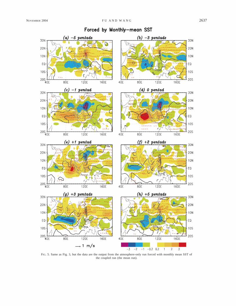
NOVEMBER 2004 2637F U A N D W A N G
FIG. 5. Same as Fig. 3, but the data are the output from the atmosphere-only run forced with monthly mean SST ofthe coupled run (the mean run).

2638 VOLUME 132M O N T H L Y W E A T H E R R E V I E W
FIG. 6. Differences of surface winds and SSTs (contour interval:0.028C) between the coupled run (Fig. 4) and the mean run (Fig. 5)at (a) 21 and (b) 13 pentads.
in the coupled run (Fig. 4c). At 0 pentad (Fig. 5d), themaximum rainfall anomaly shifts to the eastern IndianOcean. Westerly wind anomalies dominate over theequatorial Indian Ocean. A wet tongue extends into thesouth of the Arabian Sea, signifying the northward prop-agation in the western Indian Ocean. The strongest neg-ative rainfall anomaly locks on the Philippine Islands.From 11 pentad to 12 pentads (Figs. 5e and 5f), thepositive equatorial rainfall moves both northward in theIndian sector and eastward into the western Pacific. Neg-ative rainfall starts to move into the equatorial IndianOcean again. At 13 pentads (Fig. 5g), a tilted positiverainfall belt forms over the Arabian Sea, Bay of Bengal,South China Sea, and the WNP. The Indian Ocean isdominated by a north–south rainfall dipole. At 15 pen-tads (Fig. 5h), major positive rainfall stays around thePhilippine Islands; the simulation in the western Pacificseems better than that in the coupled run. The negativerainfall along the equator shifts to the eastern IndianOcean and Maritime Continent. Generally speaking, thegross spatiotemporal evolutions of the BSISO in thisatmosphere-only run are similar to those in the coupledrun and the observations except with weaker amplitudesand less coherent spatial patterns.
This result suggests that the major characteristics ofthe BSISO are very likely determined by atmosphericinternal dynamics (Wang and Xie 1997). The interac-tions between the BSISO and underlying ocean pri-marily increase the intensity of the BSISO and maintaina more coherent spatiotemporal evolution. The strongerintensity in the coupled run implies that the SST fluc-tuations associated with the BSISO do feed back to theconvection positively (Fu et al. 2003). We have com-pared the SST anomaly pattern and surface wind dif-ferences between the coupled run and the mean run from25 to 15 pentads. At 21 pentad and 13 pentads, theSST gradient seems to significantly contribute to thesurface wind differences. At 21 pentad (Fig. 6a), apositive SST patch situates in the central Indian Ocean,with a negative SST over the Bay of Bengal and SouthChina Sea. A cyclonic (anticyclonic) circulation is col-located with a warm (cold) SST patch with air flowingfrom the cold region to the warm region. A similarscenario appears at 13 pentads (Fig. 6b). A negativeSST anomaly region tilts northwest and southeast in thecentral Indian Ocean and a positive SST anomaly existsover the Bay of Bengal and the South China Sea. Acyclonic (anticyclonic) circulation is over the positive(negative) SST anomaly region. It suggests that the SST-gradient anomalies associated with the BSISO couldfeed back to the convection through changing theboundary layer winds (Lindzen and Nigam 1987).
4. The NPISO in the Indian sector
a. The wavenumber-frequency analysis of the NPISO
As indicated in the previous section, one dominantmode of the BSISO in the Indian sector is the NPISO.
The disturbances initiated at (or migrated to) the equa-torial Indian Ocean tend to propagate northward intothe south Asian continent in boreal summer (Yasunari1979). The better simulation of this intraseasonal modemay improve the predictability of active (break) spellsof the south Asian summer monsoon. Following Wheel-er and Kiladis (1999) and Teng and Wang (2003), thewavenumber-frequency analysis has been used to sum-marize the meridional propagating disturbances between108S and 308N for 10 boreal summers in the Indiansector. Figure 7 presents the 10-yr mean spectral densityaveraged in a zonal band extending from 658 to 958Efor the observations (CMAP), the coupled run, and twoatmosphere-only runs. In Figs. 7a–d, the northward-propagating variances significantly dominate over theirsouthward-propagating counterparts. The periods for thedominant northward-propagating variability are 40–50days with their wavelengths about 408 in latitude. Thepropagating speed is about 1 m s21. The simulated NPI-SO (particularly in the coupled run and daily run; Figs.7b and 7c) is a bit slower (or with a longer period) thanthat in the CMAP observations. The intensity of theNPISO is strongest in the coupled run (even a bit stron-ger than the observations) and weakest in the mean run,with the intensity of the daily run in between. The sim-ilarity of the three runs does suggest that the atmosphericinternal dynamics alone could produce a dominant NPI-SO in boreal summer over the Indian sector. Includingintraseasonal SST forcing or active air–sea coupling ba-

NOVEMBER 2004 2639F U A N D W A N G
FIG. 7. Wavenumber-frequency spectra of rainfall rate associated with the NPISOs averaged between 658 and 958Efor (a) the observations (CMAP), (b) the coupled run (taken from Fig. 4a in Fu et al. 2003), (c) the atmosphere-onlyrun forced with daily mean SST, and (d) the atmosphere-only run forced with monthly mean SST. The contour intervalis 3 (mm day21)2.

2640 VOLUME 132M O N T H L Y W E A T H E R R E V I E W
sically increases the intensity of the NPISO, probablyslowing down the NPISO a little bit, but has no sig-nificant impacts on its meridional scale (or wavelength).If just comparing the intensity of the NPISO in the threeruns, one may argue that the daily run is more realisticthan the coupled run. In the following subsection, theanalyses of the phase relationships will suggest the op-posite.
b. Phase relationships of the NPISO
In section 3a, we documented the coherent evolutionsof surface winds, SST, and rainfall associated with theBSISO in the entire Asia–western Pacific region. Here,we focus on the NPISO in the Indian sector and furtherexamine the phase relationships among rainfall, SST,surface divergence, vorticity, net surface heat flux (Qnet),solar radiation (Qsw), and latent heat flux (Qlat). Lagcorrelation is used to document these phase relationshipswith 10 summers’ data. We take surface heat flux asbeing positive into the ocean. Therefore, a positive Qlat
anomaly represents less evaporation from ocean to at-mosphere. All correlation coefficients are averaged be-tween 658 and 958E to represent the large-scale featurein the Indian sector.
Figures 8 and 9 compare the lag correlations of sixpairs of variables for the observations and the coupledsolution. The observed surface divergence and vorticityare calculated from the ECMWF surface winds. Figures8a and 9a show that, in the northern Indian Ocean, pos-itive (negative) SST fluctuations lead (lag) convectionby about two pentads. Surface convergence is almostin phase with convection from 208S to 208N (Figs. 8band 9b), indicating the strong coupling between con-vection and surface convergence. Figures 8c and 9cshow that positive surface vorticity leads convectionwith two pentads to 2 days between the equator and158N. These results suggest that both positive SST andpositive vorticity work together to lead the equatorialdisturbances to move northward. Regarding the phaserelationships between the convection and surface heatfluxes, the major difference between the ECMWF anal-ysis and the coupled run is the latent heat fluxes (Figs.8f and 9f). The maximum surface evaporation lags con-vection by 3–4 days in the analysis (Fig. 8f) but isalmost in phase with each other in the coupled run (Fig.9f). Because the minimum solar radiation collocateswith the convection in both cases (Figs. 8e and 9e), theresultant minimum net surface heat flux lags the con-vection in the analysis (Fig. 8d) but is almost in phasein the coupled run (Fig. 9d).
The phase difference of latent heat fluxes between thecoupled model and ECMWF analysis may not imme-diately lead to the conclusion that the modeling latentheat flux is wrong. There are several issues that needto be resolved before we could make a final conclusion.First, the above so-called observations of surface heatfluxes are taken from the ECMWF analysis rather than
from in situ observations. Second, the in-phase rela-tionship between convection and the maximum evap-oration was observed in JASMINE (Webster et al.2002), though only one NPISO event was captured.Third, Inness and Slingo (2003) found the same kindof phase difference as we found here when they com-pared their MJO simulations in the Third Hadley CentreCoupled Ocean–Atmosphere GCM (HadCM3) withthose in the ECMWF reanalysis. They showed that, overthe Indian Ocean, the maximum evaporation lags con-vection by 3–4 days in the ECMWF reanalysis but isin phase in the HadCM3. In addition, both kinds ofphase relationships in the ECMWF analysis (Fig. 8f)and our coupled model (Fig. 9f) were observed in thewestern Pacific by the TOGA COARE and Tropical At-mosphere Ocean (TAO) array (Zhang and McPhaden2000) with respect to the eastward-moving MJO. Ap-parently, more in situ observations in the Indian Oceanare needed to clarify the above discrepancies.
For the two atmosphere-only runs, the lag correlationsamong rainfall, surface circulations, and heat fluxes arealmost the same as those in the coupled run. To savespace, no figures are repeated here. However, as wefound in the Arabian Sea and Bay of Bengal (Fu et al.2003), the phase relationship between the rainfall andSST over the Indian Ocean in the daily run (Fig. 10) isquite different from those in the coupled run and theobservations. Instead of a quadrature phase relationship(Figs. 8a and 9a), the intraseasonal SST in this forcedatmospheric run (Fig. 10) is almost in phase with theconvection near the equator and shows a slight lead ofthe convection by about 2–3 days in the northern IndianOcean with a maximum correlation coefficient about 0.3(only half of that in the coupled run). This result in-dicates that the air–sea coupling will not significantlychange the phase relationships between the convectionand surface circulations and heat fluxes. On the otherhand, it further supports the conclusion that the BSISOsolution in the coupled run is more realistic than thatin the forced atmospheric run. The possible impacts ofair–sea coupling on the predictability of the BSISO arediscussed in the last section.
c. Vertical structures of the NPISO
In order to validate the vertical structures of the sim-ulated NPISO, a composite analysis is used to constructthe vertical structures from the ECMWF analysis andthe coupled solution. To select the composite events,two criteria are applied to the filtered rainfall data av-eraged between 858 and 958E: 1) a positive rainfallanomaly continuously moves northward at least fromthe equator to 108N; 2) in the course of the northwardprogression, the positive rainfall anomaly larger than 5mm day21 must extend more than 108 in latitude. Oncea case is selected, its reference pentad (0) is set at thetime when the northward-propagating rainfall anomalyreaches its maximum at 108N. With the same criteria,

NOVEMBER 2004 2641F U A N D W A N G
FIG. 8. Lag correlations, averaged over 658 to 958E, between rainfall and (a) SST, (b) surface divergence, (c) surfacevorticity, (d) net surface heat flux, (e) downward solar radiation, and (f ) surface latent heat flux for 10 boreal summers(1991–2000). Data are from CMAP, ECMWF analysis, and Reynolds SST.

2642 VOLUME 132M O N T H L Y W E A T H E R R E V I E W
FIG. 9. Same as Fig. 8, but the data are the output from the coupled run.

NOVEMBER 2004 2643F U A N D W A N G
FIG. 10. Lag correlations of rainfall and SST averaged over 658and 958E for the atmosphere-only run forced by the daily SST fromthe coupled run.
15 events are qualified for the observations (CMAP,1991–2000), 16 events for the coupled solution, 13events for the atmosphere-only solution forced with dai-ly mean SST, and 5 events for the atmosphere-only so-lution forced with monthly mean SST. This result in-dicates that the coupled run produces many more strongnorthward-propagating events than the mean atmospher-ic run.
Figure 11 shows the rainfall and SST anomalies as-sociated with the composite NPISO for the observations,the coupled run, and the mean run. No significant SSTanomaly appears in the mean run (Fig. 11c) because ofthe use of monthly mean SST as boundary forcing. Thecomposite rainfall anomalies in both the mean run (5cases) and the coupled run (15 cases) show coherentnorthward propagation as in the observations. In boththe observations and the coupled run (Figs. 11a and11b), the composite positive SST anomalies lead thewet phase by a quarter of an ISO cycle with a magnitudeabout 0.258C near the south Bay of Bengal (about 148N).In the daily run (figure not shown), the composite rain-fall is similar to those in the mean run and the coupledrun, while the amplitude of the composite SST anomalyis smaller than that in the coupled run with the SSTleading the convection by about 3 days (Fig. 10). In thecoupled run, the dry phase that follows the wet phaseis relatively weak compared to the observations. Thesimulated negative SST anomaly is also smaller and lagsthe observations in the northern Indian Ocean (from 88to 158N), suggesting the oceanic cooling associated with
active ISO phase is smaller in the model. The possiblecause is discussed later.
Figures 12 and 13 compare the composite verticalstructures of moisture and circulations associated withthe NPISO at 23, 21, 0, 11, 13 pentads from ECMWFanalysis and the coupled solution. At 23 pentads, thestrongest convection appears near the equator in bothECMWF analysis and the coupled solution (Figs. 12aand 13a). The convection, associated with ascendingmotion, moistens the entire troposphere with maximummoisture perturbation around 700 hPa; the magnitudeof maximum moisture perturbations (both the positiveand the negative) in the coupled solution is considerablylarger than that in the analysis. In contrast to the anal-ysis, a negative moisture anomaly is found near thesurface at the equator in the coupled run, suggestingthat excessively strong dry downdrafts penetrate to thesurface in the model. Over the northern Indian Ocean,strong descending motion and tropospheric drying arepresent in both the observations and the simulation, withthe latter having a larger meridional scale. A close me-ridional circulation, with a first-baroclinic-mode struc-ture, connects the wet and dry phases of the NPISOtogether, implying that positive feedback may exist be-tween the wet and dry zones through a local Hadleycirculation (Lau and Peng 1990). Two pentads later (21pentad), the strongest convection moves northward withthe ascending branch around 58N (Figs. 12b and 13b).The associated descending branch and drying regionalso moves northward. Dissimilar to the analysis, themodel produces a negative moisture anomaly near thesurface in the rainy region and a dry zone in the lowertroposphere just south of the equator. The temperatureanomalies (Figs. 14a and 14b) at this time show twovertical nodes in the rainy region: positive anomaliesbelow 850 hPa and between 600 and 200 hPa; negativeanomalies above 200 hPa and between 850 and 600 hPa.In the drying region over the northern Indian Ocean,one node dominates with positive anomalies below 500hPa and negative anomalies above. The vertical struc-ture and the magnitude of the air temperature anomaliesare very similar between the ECMWF analysis and thecoupled solution. Ahead of the convection, the com-bination of boundary layer positive air temperatureanomaly and the drying in the troposphere destabilizesthe atmosphere and favors the northward movement ofthe convection. The positive SST anomalies in the north-ern Indian Ocean warm the boundary layer through ver-tical mixing, thus contributing to the northward prop-agation. This boundary layer warming process ahead ofthe convection is not seen in the atmosphere-only runforced by monthly mean SST (Fig. 14c).
At 0 pentad (Figs. 12c and 13c), the convection movesto 108N in the coupled solution, slightly north of 108Nin the ECMWF analysis. Two dry zones appear in thenorth and south sides of the rainy region. The ascendingair associated with convection starts to descend in bothnorth and south sides. Two meridional cells form. At

2644 VOLUME 132M O N T H L Y W E A T H E R R E V I E W
FIG. 11. Composite rainfall (mm day21; shaded) and SST (contours; contour interval: 0.058C)associated with the NPISOs averaged between 858 and 958E in (a) the observations (15 events),(b) the coupled run (16 events), and (c) the mean run (5 events).
11 pentad (Figs. 12d and 13d), the south meridionalcell starts to intensify and the north one is weakening.The wet phase occupies almost the entire northern In-dian Ocean. At 13 pentads, the equatorial dry zoneassociated with descending motion quickly moves intothe northern Indian Ocean in the ECMWF analysis (Fig.12e); the wet zone moves to the north of 158N. Thecoupled solution also indicates the northward intrusionof the dry zone (Fig. 13e); however, the wet phase doesnot decay as quickly and moves as north as that in the
analysis. From 23 pentads to 13 pentads (Figs. 12 and13), the northward progression of the moisture maxi-mum associated with the NPISO is slower in the coupledmodel (from 28S to 178N) than that in the analysis (from38S to 228N).
One possible reason for the slow northward move-ment of the wet phase in the coupled model is the in-adequate simulation of sea surface cooling associatedwith the strong convection in the Bay of Bengal (Figs.4h and 11b). The composite SST cooling in the Bay of

NOVEMBER 2004 2645F U A N D W A N G
FIG. 12. Composite vertical structures of moisture (contour interval:0.1 g kg21; positive contours shaded) and circulation perturbationsassociated with the NPISO in the observations at (a) 23, (b) 21, (c)0, (d) 11, and (e) 13 pentads.
Bengal (148N, 908E) occurs much faster in the obser-vations than in the coupled run (Fig. 15b). From 21pentad to 13 pentads, the accumulated negative surfaceheat flux in the analysis is obviously smaller than thatin the coupled model (Fig. 15a). However, the SST dropsabout 0.558C in the analysis and only 0.348C in themodel. In the entire composite cycle, the change of netsurface heat flux in the coupled model is actually largerthan that in the analysis, while the SST response in thecoupled model is smaller, indicating the mixed layer inthe model is too deep. If we increase the modeled SSTvariation by a coefficient of 1.4 (equivalent to a reduc-tion of the mixed-layer depth by about 30%), SST am-plitudes become similar between the coupled model andthe observations.1 However, the cooling of sea surfacein the model is still too slow compared to the analysis.This suggests that the weak cooling rate is not only dueto the systematic error in the mixed-layer depth in thecoupled model, but particularly in the cooling period.One possible cause of the weak cooling is the lack ofsalinity effects in the ocean model. The data from JAS-MINE suggest that a shallow barrier layer forms in theconvective phase (Webster et al. 2002). The depth ofthe barrier layer is about 10–20 m shallower than thethermal mixed layer. The shallow barrier layer increasesthe efficiency of the negative surface heat flux on cool-ing the sea surface (Lukas and Lindstrom 1991). There-fore, better representations of salinity effects in theocean model are needed to improve the simulation ofthe BSISO.
For the atmosphere-only runs, the composite verticalstructures of moisture and circulations at 23, 21, 0,11, 13 pentads associated with the NPISO are similarto those from the coupled run (figure not shown). Thecommon discrepancies with the ECMWF analysis forboth the atmospheric runs and the coupled run are 1)tropospheric moisture fluctuations associated with theNPISO are too large and 2) negative surface moistureperturbations occur in the convective phase of the NPI-SO.
5. Summary and discussion
We have validated the boreal-summer intraseasonaloscillation (BSISO) simulated by a hybrid-coupledmodel with the ECMWF analysis, CMAP rainfall, andReynolds’ SST. The model captures the large-scale fea-tures (e.g., circulations and rainfall) of the Asia–westernPacific summer monsoon (Fig. 1) and the major vari-ability centers of the BSISO (Fig. 2) but also has somesystematic errors (e.g., too strong rainfall over the Phil-ippine Islands and too weak rainfall in the WNP). The
1 Considering that the magnitude of SST fluctuations in the Reyn-olds’ dataset is smaller than that in the TMI data and buoy data overthe Bay of Bengal (Vecchi and Harrison 2002; Sengupta et al. 2001),more studies are needed to improve our understanding and represen-tation of the processes governing the SST variations in this area.
observational data (or model analysis) were used to re-veal the coherent spatiotemporal evolutions among theconvection, atmospheric circulations, and underlyingSST of the BSISO (Fig. 3). The coupled model repro-duces the observed spatiotemporal evolutions in mostof the phases (Fig. 4). Focusing on the Indian sector,the coupled model is able to produce a NPISO with itsintensity and dominant period (or propagating speed)all resembling closely those derived from CMAP rain-fall (Fig. 7). The lag correlations between the NPISOrainfall and underlying SST, surface convergence, vor-ticity, and surface heat fluxes suggest that both positiveSST and vorticity perturbations act to lead the equatorialdisturbances to move northward (Figs. 8 and 9).
A few obvious discrepancies between the coupledsolution and the observations are also noticed. First, theocean component of this coupled model produces very

2646 VOLUME 132M O N T H L Y W E A T H E R R E V I E W
FIG. 13. Same as Fig. 12, but the data are the output from thecoupled run.
FIG. 14. Composite vertical structures of air temperature pertur-bations (contour interval: 0.18C; positive contours shaded) at 21pentad for (a) the ECMWF analysis, (b) the coupled run, and (c) themean run.
slow mixed-layer cooling during the active phase of theBSISO, particularly in the Bay of Bengal and SouthChina Sea (Figs. 4h and 15b). We speculate that the lackof salinity effects in the ocean model is the primarycause. The precipitation associated with the active phaseof the ISO develops a shallow barrier layer, which couldconsiderably increase the efficiency of mixed-layercooling (Lukas and Lindstrom 1991). This process ismissing in our current ocean model. Second, the phaserelationship between latent heat flux and rainfall isslightly different in the coupled solution (Fig. 9f) andin the ECMWF analysis (Fig. 8f). As we discussed insection 4b, more accurate surface latent heat flux ob-servations are needed to pin down the causes of thisdiscrepancy. Third, the tropospheric moisture fluctua-tions associated with the NPISO in the coupled solution(also the atmosphere-only solutions) are too large com-pared to those from the ECMWF analysis (Figs. 12 and
13). The near-surface negative moisture perturbationsin the convective phase of the BSISO (Figs. 13a and13b) suggest that the downdrafts in the ECHAM4 GCMare overestimated.
The intercomparison between the coupled run andtwo atmospheric runs (the mean and daily runs) suggeststhat the atmosphere–ocean coupled system is the ulti-mate tool needed to realistically simulate the BSISO.The coupled run produces the most coherent spatiotem-poral evolutions among the convection, the associatedcirculations, and underlying SST (Figs. 4 and 5). It alsohas the strongest intensity of the NPISO (Fig. 7) andmaintains a correct phase relationship between the con-vection and SST (Figs. 4 and 9a). The composite anal-ysis reveals that the number of strong NPISOs in thecoupled run (16 events; 15 events in the observations)is many more than that in the mean run (5 events; 13events in the daily run). The better simulation in thecoupled system is largely attributed to the coherent SSTfluctuations associated with the BSISO (Figs. 3 and 4).The intraseasonal SST fluctuations feed back to the con-vection possibly through changing the convective in-stability (Fig. 14) and SST-gradient forced surfacewinds (Fig. 6). On the other hand, the similarities amongthe three runs [e.g., the spatiotemporal evolutions ofrainfall and surface winds (Fig. 5); the characteristicsand vertical structures of the NPISO (Figs. 7 and 13);the phase relationships between convection and surfaceheat fluxes (Fig. 9)] do point out the critical role of aGCM’s internal dynamics on the reasonable simulation

NOVEMBER 2004 2647F U A N D W A N G
FIG. 15. Composite intraseasonal cycle of (a) net surface heat flux anomalies (W m22) and(b) SST anomalies (8C) at the Bay of Bengal (148N, 908E) from the observations and thecoupled run.
of the BSISO. In contrast to traditional wisdom aboutthe power of SST as an external boundary forcing inthe seasonal and interannual time scales, the atmo-sphere-only run forced by high-frequency (e.g., daily)SST very likely produces a most unphysical solution ofthe BSISO compared to the coupled run and the meanrun. In the mean run, the simulated BSISO is purelydetermined by the internal atmospheric dynamics (in-cluding active land–atmosphere interaction). In the cou-pled system, the feedback between the internal atmo-
spheric dynamics and underlying sea surface is realis-tically reflected. For the daily run, most likely, the high-frequency SST interferes with the internal atmosphericdynamics associated with the BSISO in an unrealisticway (Figs. 8a, 9a, and 10).
Finally, the different phase relationship between theconvection and SST associated with the BSISO in acoupled system and an atmosphere-only system prob-ably has important implications to the predictability ofthe BSISO. In the coupled system, the positive SST

2648 VOLUME 132M O N T H L Y W E A T H E R R E V I E W
systematically leads the convection by about 10 days(as in the observations). The intraseasonal SST in thecoupled system may serve as a memory to extend thepredictability of the BSISO, while the intraseasonal SSTin the atmosphere-only system very likely acts as a falseexternal boundary forcing (Wu et al. 2002; Waliser etal. 2003c, 16–19; Fu and Wang 2004). If the interactionbetween the convection and large-scale circulations(purely internal atmospheric dynamics) can give a usefulBSISO prediction of about 15 days (Waliser et al.2003b), the SST signal forced by the convection andlarge-scale circulations in a coupled system might ex-tend our predictability to about 1 month. This hypothesisis under investigation.
Acknowledgments. The authors appreciate Drs. L.Bengtsson, E. Roeckner, L. Dumenil, and U. Schulzweidaat the Max Planck Institute for Meteorology for theirkind help in the implementation of ECHAM4 GCM atthe IPRC. XF thanks R. Lukas for helpful discussions.This research was supported by the NASA Earth ScienceProgram, NSF Climate Dynamics Program, and by theJapan Agency for Marine–Earth Science and Technol-ogy (JAMSTEC) through its sponsorship of the IPRC.
REFERENCES
Bhat, G. S., and Coauthors, 2001: BOBMEX: The Bay of BengalMonsoon Experiment. Bull. Amer. Meteor. Soc., 82, 2217–2243.
Blade, I., and D. L. Hartmann, 1993: Tropical intraseasonal oscil-lations in a simple nonlinear model. J. Atmos. Sci., 50, 2922–2939.
Chang, C.-P., 1977: Viscous internal gravity waves and low-frequencyoscillations in the Tropics. J. Atmos. Sci., 34, 901–910.
Flatau, M., P. Flatau, P. Phoebus, and P. Niller, 1997: The feedbackbetween equatorial convection and local radiative and evapo-rative processes: The implications for intraseasonal oscillations.J. Atmos. Sci., 54, 2373–2386.
Fu, X., and B. Wang, 2001: A coupled modeling study of the annualcycle of the Pacific cold tongue. Part I: Simulation and sensitivityexperiments. J. Climate, 14, 765–779.
——, and ——, 2004: Differences of boreal-summer intraseasonaloscillations simulated in an atmosphere–ocean coupled modeland an atmosphere-only model. J. Climate, 17, 1263–1271.
——, ——, and T. Li, 2002: Impacts of air–sea coupling on thesimulation of mean Asian summer monsoon in the ECHAM4model. Mon. Wea. Rev., 130, 2889–2903.
——, ——, ——, and J. P. McCreary, 2003: Coupling between north-ward-propagating, intraseasonal oscillations and sea surface tem-perature in the Indian Ocean. J. Atmos. Sci., 60, 1733–1753.
Gadgil, S., and S. Sajani, 1998: Monsoon precipitation in the AMIPruns. Climate Dyn., 14, 659–689.
Gaspar, P., 1988: Modeling the seasonal cycle of the upper ocean. J.Phys. Oceanogr., 18, 161–180.
Grabowski, W. W., 2003: MJO-like coherent structures: Sensitivitysimulations using the cloud-resolving convective parameteri-zation. J. Atmos. Sci., 60, 847–864.
Hayashi, Y., 1982: Space–time spectral analysis and its applicationsto atmospheric waves. J. Meteor. Soc. Japan, 60, 156–171.
Hendon, H. H., 2000: Impact of air–sea coupling on the Madden–Julian oscillation in a general circulation model. J. Atmos. Sci.,57, 3939–3952.
——, and M. L. Salby, 1994: The life cycle of the Madden–Julianoscillation in a general circulation model. J. Atmos. Sci., 51,2225–2237.
Hu, Q., and D. A. Randall, 1994: Low-frequency oscillations in ra-diative–convective systems. J. Atmos. Sci., 51, 1089–1099.
Inness, P. M., and J. M. Slingo, 2003: Simulation of the Madden–Julian oscillation in a coupled general circulation model. Part I:Comparison with observations and an atmosphere-only GCM.J. Climate, 16, 345–364.
Kang, I.-S., C.-H. Ho, Y.-K. Lim, and K.-M. Lau, 1999: Principalmodes of climatological seasonal and intraseasonal variations ofthe Asian summer monsoon. Mon. Wea. Rev., 127, 322–340.
——, and Coauthors, 2002: Intercomparison of the climatologicalvariations of Asian summer monsoon precipitation simulated by10 GCMs. Climate Dyn., 19, 383–395.
Kawamura, R., R. T. Murakami, and B. Wang, 1996: Tropical andmidlatitude 45-day perturbations during the northern summer. J.Meteor. Soc. Japan, 74, 867–890.
Kemball-Cook, S., and B. Wang, 2001: Equatorial waves and air–seainteraction in the boreal summer intraseasonal oscillation. J. Cli-mate, 14, 2923–2942.
——, ——, and X. Fu, 2002: Simulation of the ISO in the ECHAM4model: The impact of coupling with an ocean model. J. Atmos.Sci., 59, 1433–1453.
Krishnamurti, T. N., 1985: Summer monsoon experiment—A review.Mon. Wea. Rev., 113, 1590–1626.
——, D. K. Oosterhof, and A. V. Mehta, 1988: Air–sea interactionon the time scale of 30 to 50 days. J. Atmos. Sci., 45, 1304–1322.
——, M. Subramaniam, G. Daughenbaugh, D. Oosterhof, and J. Xue,1992: One-month forecasts of wet and dry spells of the monsoon.Mon. Wea. Rev., 120, 1191–1223.
Lau, K. M., and P. H. Chan, 1986: Aspects of the 40–50 day oscil-lation during the northern summer as inferred from outgoinglongwave radiation. Mon. Wea. Rev., 114, 1354–1367.
——, and L. Peng, 1987: Origin of low frequency (intraseasonal)oscillations in the tropical atmosphere. Part I: The basic theory.J. Atmos. Sci., 44, 950–972.
——, and ——, 1990: Origin of low frequency (intraseasonal) os-cillations in the tropical atmosphere. Part III: Monsoon dynam-ics. J. Atmos. Sci., 47, 1443–1462.
——, K. M. Kim, and S. Yang, 2000: Dynamical and boundary forc-ing characteristics of regional components of the Asian summermonsoon. J. Climate, 13, 2461–2482.
Lee, M. I., I.-S. Kang, J.-K. Kim, and B. E. Mapes, 2001: Influencesof cloud–radiation interaction on simulating tropical intrasea-sonal oscillation with an atmospheric general circulation model.J. Geophys. Res., 106, 14 219–14 233.
Lindzen, R. S., and S. Nigam, 1987: On the role of sea surfacetemperature gradients in forcing low-level winds and conver-gence in the Tropics. J. Atmos. Sci., 45, 2440–2458.
Lukas, R., and E. Lindstrom, 1991: The mixed layer of the westernequatorial Pacific Ocean. J. Geophys. Res., 96, 3343–3357.
Madden, R. A., and P. R. Julian, 1971: Detection of a 40–50 dayoscillation in the zonal wind in the tropical Pacific. J. Atmos.Sci., 28, 702–708.
Maloney, E. D., and D. L. Hartmann, 2001: The sensitivity of intra-seasonal variability in the NCAR CCM3 to changes in convectiveparameterization. J. Climate, 14, 2015–2034.
McCreary, J. P., and Z. J. Yu, 1992: Equatorial dynamics in a 2.5-layer model. Progress in Oceanography, Vol. 29, Pergamon, 61–132.
Mo, K. C., 2000: Intraseasonal modulation of summer precipitationover North America. Mon. Wea. Rev., 128, 1490–1505.
Myers, D. S., and D. E. Waliser, 2003: Three-dimensional water vaporand cloud variations associated with the Madden–Julian oscil-lation during Northern Hemisphere winter. J. Climate, 16, 929–950.
Neelin, D. J., and J. Y. Yu, 1994: Modes of tropical variability underconvective adjustment and the Madden–Julian oscillation. PartI: Analytical theory. J. Atmos. Sci., 51, 1876–1894.
Nordeng, T. E., 1994: Extended version of the convective parame-terization scheme at ECMWF and their impact on the mean and

NOVEMBER 2004 2649F U A N D W A N G
transient activity of the model in the Tropics. ECMWF ResearchDepartment Tech. Memo. 206, European Centre for Medium-Range Weather Forecasts, Reading, United Kingdom, 41 pp.
Rajendran, K., A. Kitoh, and O. Arakawa, 2004: Monsoon low-fre-quency intraseasonal oscillation and ocean–atmosphere couplingover the Indian Ocean. Geophys. Res. Lett., 31, L02210, doi:10.1029/2003GL019031.
Raymond, D. J., 2001: A new model of the Madden–Julian oscillation.J. Atmos. Sci., 58, 2807–2819.
Reynolds, R. W., and T. M. Smith, 1994: Improved global sea surfacetemperature analyses using optimum interpolation. J. Climate,7, 929–948.
Roeckner, E., and Coauthors, 1996: The atmospheric general circu-lation model ECHAM4: Model description and simulation ofpresent-day climate. Max Planck Institute for Meteorology Rep.218, 90 pp.
Rui, H., and B. Wang, 1990: Development characteristics and dy-namic structure of tropical intraseasonal convection anomalies.J. Atmos. Sci., 47, 357–379.
Sengupta, D., B. N. Goswami, and R. Senan, 2001: Coherent intra-seasonal oscillations of ocean and atmosphere during the Asiansummer monsoon. Geophys. Res. Lett., 28, 4127–4130.
Slingo, J. M., and Coauthors, 1996: Intraseasonal oscillations in 15atmospheric general circulation models: Results from an AMIPdiagnostic subproject. Climate Dyn., 12, 325–357.
Sperber, K. R., J. M. Slingo, P. M. Inness, and K. M. Lau, 1997: Onthe maintenance and initiation of the intraseasonal oscillation inthe NCEP/NCAR reanalysis and the GLA and UKMO AMIPsimulations. Climate Dyn., 13, 769–795.
Taylor, K. E., D. Williamson, and F. Zwiers, 2000: The sea surfacetemperature and sea-ice concentration boundary condition forAMIP II simulations. PCMDI Rep. 60, Program for Climate ModelDiagnosis and Intercomparison, Lawrence Livermore NationalLaboratory, Livermore, CA, 25 pp. [Available online at http://www-pcmdi.llnl.gov/amip/AMIP2EXPDSN/BCS/amip2bcs.html.]
Teng, H., and B. Wang, 2003: Interannual variations of the borealsummer intraseasonal oscillation in the Asian–Pacific region. J.Climate, 16, 3572–3584.
Tiedtke, M., 1989: A comprehensive mass flux scheme for cumulusparameterization in large-scale models. Mon. Wea. Rev., 117,1779–1800.
Tokioka, T., K. Yamazaki, A. Kitoh, and T. Ose, 1988: The equatorial30–60 day oscillation and the Arakawa–Schubert penetrativecumulus parameterization. J. Meteor. Soc. Japan, 66, 883–901.
Tompkins, A. M., 2001: On the relationship between tropical con-vection and sea surface temperature. J. Climate, 14, 633–637.
Vecchi, G., and D. E. Harrison, 2002: Monsoon breaks and subsea-sonal sea surface temperature variability in the Bay of Bengal.J. Climate, 15, 1485–1493.
Waliser, D. E., K. M. Lau, and J. H. Kim, 1999: The influence ofcoupled sea surface temperatures on the Madden–Julian oscil-lation: A model perturbation experiment. J. Atmos. Sci., 56, 333–358.
——, and Coauthors, 2003a: AGCM simulations of intraseasonalvariability associated with the Asian summer monsoon. ClimateDyn., 21, 423–446.
——, K. M. Lau, W. Stern, and C. Jones, 2003b: Potential predict-
ability of the Madden–Julian oscillation. Bull. Amer. Meteor.Soc., 84, 1191–1196.
——, S. Schubert, A. Kumar, K. Weickmann, and R. Dole, 2003c:Proc. Workshop on Modeling, Simulation and Forecasting ofSubseasonal Variability. Vol. 25, NASA/CPC-2003-104606,College Park, MD, NASA.
Wang, B., 1988: Dynamics of tropical low-frequency waves: An anal-ysis of the moist Kelvin wave. J. Atmos. Sci., 45, 2051–2065.
——, and H. Rui, 1990: Synoptic climatology of transient tropicalintraseasonal convection anomalies: 1975–1985. Meteor. Atmos.Phys., 44, 43–61.
——, and X. Xie, 1996: Low-frequency equatorial waves in shearedzonal flow. Part I: Stable waves. J. Atmos. Sci., 53, 449–467.
——, and ——, 1997: A model for the boreal summer intraseasonaloscillation. J. Atmos. Sci., 54, 72–86.
——, and ——, 1998: Coupled modes of the warm pool climatesystem. Part I: The role of the air–sea interaction in maintainingthe Madden–Julian oscillation. J. Climate, 11, 2116–2135.
——, T. Li, and P. Chang, 1995: An intermediate model of the tropicalPacific Ocean. J. Phys. Oceanogr., 25, 1599–1616.
Wang, W., and M. E. Schlesinger, 1999: The dependence on con-vection parameterization of the tropical intraseasonal oscillationsimulated by the UIUC 11-layer atmospheric GCM. J. Climate,12, 1423–1457.
Webster, P. J., 1983: Mechanisms of monsoon low-frequency vari-ability: Surface hydrological effects. J. Atmos. Sci., 40, 2110–2124.
——, and R. Lukas, 1992: TOGA COARE: The Coupled Ocean–Atmosphere Response Experiment. Bull. Amer. Meteor. Soc., 73,1377–1416.
——, V. O. Magana, T. N. Palmer, J. Shukla, R. A. Tomas, M. Yanai,and T. Yasunari, 1998: Monsoons: Processes, predictability, andthe prospects for prediction. J. Geophys. Res., 103C, 14 451–14 510.
——, and Coauthors, 2002: The JASMINE pilot study. Bull. Amer.Meteor. Soc., 83, 1603–1629.
Wheeler, M., and G. N. Kiladis, 1999: Convectively coupled equa-torial waves: Analysis of clouds and temperature in the wave-number-frequency domain. J. Atmos. Sci., 56, 374–399.
Wu, M. L. C., S. Schubert, I. S. Kang, and D. E. Waliser, 2002:Forced and free intraseasonal variability over the south Asianmonsoon region simulated by 10 AGCMs. J. Climate, 15, 2862–2880.
Xie, P., and P. A. Arkin, 1997: Global precipitation: A 17-year month-ly analysis based on gauge observations, satellite estimates, andnumerical model outputs. Bull. Amer. Meteor. Soc., 78, 2539–2558.
Yasunari, T., 1979: Cloudiness fluctuations associated with the North-ern Hemisphere summer monsoon. J. Meteor. Soc. Japan, 57,227–242.
Zhang, C., 1996: Atmospheric intraseasonal variability at the surfacein the tropical western Pacific ocean. J. Atmos. Sci., 53, 739–758.
——, and M. J. McPhaden, 2000: Intraseasonal surface cooling inthe equatorial western Pacific. J. Climate, 13, 2261–2276.
Zheng, Y., D. E. Waliser, W. F. Stern, and C. Jones, 2004: The roleof coupled sea surface temperatures in the simulation of thetropical intraseasonal oscillation. J. Climate, 17, 4109–4134.