the bootstrap s-chart for process variability: an

Journal of Quality and Technology Management Volume X, Issue II, December 2014, Page 81 – 96

THE BOOTSTRAP S-CHART FOR PROCESS VARIABILITY: AN ALTERNATIVE TO MAD CHART

N. Saeed, S. Kamal

College of Statistical and Actuarial Sciences, University of the Punjab, Lahore

ABSTRACT In statistical process control, the control charts are the most powerful tools for assessing the process behaviour. The Shewhart S chart is a standard tool for determining process variability. Similar to S chart, the chart based on Median Absolute Deviation from the sample median namely MAD estimator is also

considered robust for both normal and non-normal processes. As

and

are considered unbiased estimators of so the process standard deviation can be estimated but the true standard deviation cannot be found because only one specific sample is considered. Under the remarkable properties of bootstrap methods, we have proposed bootstrap S chart through which the true process standard deviation can be estimated. The performance of proposed chart is estimated on the basis of in-control average run length, coverage probability and confidence width. As a result the proposed chart has performed better than the traditional S and MAD charts under the assumption of normality. The simulation study based on monte-carlo runs is conducted for the purpose and the application on a practical data set is also discussed to justify the findings. Keywords: Average Run Length (ARL), bootstrap, coverage probability, interval width, Median Absolute Deviation about median (MAD).

1) INTRODUCTION The control charts are standard tools for measuring the process performance (Liu and Tang, 1996). These were developed in 1920‟s and now they have become powerful tools in statistical process control (Shewhart, 1931). When dealing with a quality characteristic, it is necessary to monitor both its mean value and the variability. Process variability can be monitored through a control chart for standard deviation, called S chart or the control chart for range, called an R chart (Montgomery, 2001). Since inherent variability in any process is always

The Bootstrap S-Chart for Process Variability: An alternative to MAD Chart

82|

present, the control charts can be used to determine when to leave the process alone (in control process) and when it needs some necessary adjustments (Grant & Leaven-Worth, 1996 and Montgomery, 2001). The S-chart is considered most useful for estimating variability if the process is generated from normal distribution but when the assumption of normality is violated, the robust estimator is needed. In the recent years, the chart based on Median Absolute Deviation about median (MAD) is considered more robust approach for estimating process variability than Shewhart S chart for both normal and non normal processes. Since a robust estimator is insensitive to changes in the underlying distribution and also resistant against the presence of outliers, it is recommended for estimating process variability for normal and non-normal processes (Shawiesh, 2008). In practice, it is difficult to estimate the correct population distribution when it is unknown. Therefore statisticians use simulation based methods. So these tools are increasingly becoming popular in Statistics (Wood 2005; Mills 2002; Simon, Atkinson, and Shevokas 1976). Such a resampling method is called “Bootstrap Method” which was developed by Efron (1979). Bootstrap methods can be used when statistical distribution of some population is unknown. Under good properties of bootstrap methods, we have recommended bootstrap S chart for

estimating process variability. Since

is an unbiased estimator of , if the

process is generated from normal distribution, the proposed estimator

based on bootstrap samples would be equal to even if the population is

not normal where estimator is simply the mean of generated from bootstrap samples because we know that the distribution of mean of any estimator would always be normal irrespective of the population distribution (application of C.L. theorem).

2) REVIEW OF LITERATURE The Shewhart S-chart is one of the most frequently used tools in process control. The S-chart is based on the process variability. The fundamental assumption in Shewhart charts is that the underlying distribution of the quality measurements should be normal but in cases when data violate the assumption of normality, the calculation of control limits is not so easy. Due to this reason the control charts based on bootstrap methods are getting popular. These methods use no distributional assumptions.

http://www.amstat.org/publications/jse/v13n3/wood.html#Mills2002

http://www.amstat.org/publications/jse/v13n3/wood.html#Simon1976

Journal of Quality and Technology Management

|83

The standard bootstrap method was introduced by Efron (1979) for estimating the sampling distribution of a given statistic. Liu and Tang (1996) discussed the bootstrap methods for estimating the control limits. It was inferred in the paper that the Shewhart standard control limits could be calculated if the sample measurements follow normal distribution. But if the assumption of normality and assumption of independence of the sample violated then the calculation of control limits was not so simple. The former case was discussed by using the bootstrap methods based on central limit theorem and the later was discussed by applying moving block bootstrap method, which was a modification of standard bootstrap. The results showed that the control limits from bootstrap methods were very close to exact limits as compared to standard control limits. Based on the findings of Liu (1996), Stomberg (2001) gave the idea of using bootstrap limits for R-chart for process variability. The paper addressed the comparison of bootstrap R limits with the traditional control limits on the basis of performance measure Average Run Length (ARL). Furthermore two types of bootstrap methods i.e. non-parametric bootstrap and Jackknife method were used for the comparison. The results showed that bootstrap methods performed better in the calculation of control limits as compared to the traditional methods for both normal and non-normal data. Liu etal (2004) extended the concept of Liu and Tang (1996) by developing a moving block bootstrap control chart for dependent multivariate data. Liu (1995) has already discussed control charts for multivariate processes. Lie etal (2004) constructed a control chart based on Principle Component Analysis (PCA), and then a modified control chart based on moving block bootstrap was determined. The control limits of modified control chart were not based on independent and identically distributed (IID) assumption. The average run length and false alarm rate were used as performance measures. The simulated data and real life data were used to illustrate the results. The results showed that the MBB was better than PCA method for weakly dependent multivariate data. The performance of control chart can be tested through performance indicators like average run length. Klein (2000) developed a modified S-control chart and the comparison was made with the traditional S-chart on the basis of average run length. The coverage probability and interval width are other performance indicators which are becoming popular. The coverage probability is confidence level for which we assume that the true


84|

parameter would lie within the calculated intervals whereas the interval width is the difference between two control limits. Wang (2009) gave some methodologies for the calculation of exact average coverage probabilities as well as the exact confidence coefficients for the confidence intervals of discrete distributions. Li etal (2011) compared different confidence intervals calculated on the basis of difference between two Poisson rates. The comparison was being made on the basis of coverage probability and interval width. The most preferable interval was that which had minimum expected confidence width with highest coverage probability. Some analytical expressions of coverage probability and the expected length of confidence interval were developed in the recent years which proved their popularity as performance indicators for the control charts (Niwitpong, 2011; Yawsaeng and Mayureesawan, 2012).

3) MATERIAL AND METHODS Let be random samples of size „m‟ where each sample is composed of a number of observations called subgroup size (n), the statistic of interest is calculated for each sample and control limits are based on that statistic. The control limits are termed as lower control limit (LCL) and upper control limit (UCL) while the control line (CL) is the central line of upper and lower limit. For example for calculating the process variability, the exact control limits based on population standard deviations are formulated as:

√ (1)

(2)

√ = (3)

where

is bias adjusting constant, √

and

√ .

The values of bias adjusting constant under subgroup sizes (n) are calculated by Montgomery (2001).

The estimator is calculated for each sample. Since

is an unbiased

estimator of process standard deviation , the control limits for S-chart can be calculated as:


|85

√

(4)

(5)

√

(6)

where

√

and

√

. The formulas are

available in most of quality related books (for further details see

Montgomery, 2001). The Median Absolute Deviation (MAD) is robust scale estimator than the sample standard deviation because it can measure the deviation from sample medians (Hampel, 1974). If we take a random sample of „n‟ observations then MAD estimator is defined as:

{| |} where MD is sample median. Shawiesh (2008) developed control limits for Shewhart S-chart using MAD estimator. Since is an unbiased estimator of (Rousseeuw & Croux, 1993), the control limits for S-chart based on MAD estimator can

be transformed as √

Finally the lower and upper control limits based on MAD estimator can be defined as:

(7)

(8)

(9) where is the correction factor. Against different subgroup sizes, the values of are calculated by Shawiesh (2008). Under subgroup size 4, 5, 10, 15, 20 and 25, the values of correction factor are 1.363, 1.206, 1.087, 1.056, 1.042, 1.033. Similarly the transformed values of

can be calculated using the values of correction factor

.


86|

3.1) Bootstrap S-chart: The bootstrap method is used to select a large number of with replacement samples from one original sample (Efron and Tibshirani, 1993). The estimator is calculated for each bootstrap sample and mean

of all is used as an estimate of . Since the bootstrap has a normal distribution (due to the central limit theorem), the control limits can easily be formed as:

(10)

(11)

(12) 3.2) Average Run Length (ARL): The Average Run Length (ARL) is a well-known measure through which the performance of control chart can be determined. An in-control run length determines the maximum number of observations within the control limits before first out of control signal appears provided that the process is actually in control. Average run length is the mean of run length if the process is repeated a large number of times. It can be computed as:

(13)

where is parameter. Within control limits for a normal process, p is approximately 0.0027 and hence the average run length is 370. The greater value of in-control average run length shows the better performance of the control chart (Montgomery, 2001). 3.3) Coverage Probability: The coverage probability is known as the confidence level of the control limits. The coverage probability is termed as: Coverage Probability (C.P) = ( (14)


|87

4) RESULTS The results are based on the simulation studies conducted in two parts. In first part the control limits of S, MAD, bootstrap S charts are computed and in the second section the simulations are applied for the calculation of average run length, confidence width of the control limits and coverage probability. 4.1) Simulation Example A: The simulation study is made for the construction of control limits. The random numbers for 30 samples (m=30) are generated from standard normal distribution under different subgroup sizes i.e. n= 4, 5, 10, 15, 20, 25. The control limits of standard S (eq. 4, 5, 6), MAD (eq. 7, 8, 9) and bootstrap S (eq. 10, 11, 12) charts are calculated in table 1 while 1000 bootstrap samples are considered for the construction of bootstrap limits. The exact control limits (eq. 1, 2, 3) are also calculated on the basis of true process standard deviation ( ) so that the comparison could easily be made. The programme is written in R-language for the purpose. The findings of table 1 showed that for a normally distributed process, the bootstrap S control limits are relatively close to the exact control limits of the process as compared to the control limits based on MAD estimator. The bootstrap S limits showed better approximation of exact limits of the process under small (n= 4, 5), moderate (n= 10, 15) and large (n= 20, 25) subgroup sizes. The supporting evidence is shown in Fig. 1 through which the comparison of the control limits can be made.


88|

Table 1: Calculation of Control Limits for N (0,1) and m = 30

Control Limits Subgroup Size

4 5 10 15 20 25

Upper Control Limit (UCL)

S MAD Exact Bootstrap-S

2.125 2.259 2.088 2.074

1.829 1.832 1.964 1.900

1.747 1.792 1.669 1.725

1.541 1.573 1.544 1.546

1.447 1.460 1.470 1.460

1.429 1.358 1.420 1.424

Central Line (CL)


0.938 0.997 0.921 0.915

0.876 0.877 0.940 0.910

1.018 1.044 0.973 1.005

0.981 1.001 0.982 0.983

0.971 0.980 0.987 0.980

0.996 0.946 0.990 0.992

Lower Control Limit (LCL)


0 0 0 0

0 0 0 0

0.289 0.296 0.276 0.286

0.4197 0.429 0.421 0.421

0.495 0.499 0.504 0.499

0.563 0.534 0.559 0.561

The three line graphs are constructed using the findings of table 1. Figure 1(a, b & c) shows the graphical representation of the simulated lower control limits, control lines and upper control limits of the S, MAD and bootstrap-S charts respectively. The exact control limits of the process are also plotted on the graph so that the comparison can be made. The lower control limits are very close to each other for three charts under study and hence also close to the exact limits of the process (Figure 1.a). The trend is same for all subgroup sizes (i.e. 4, 5, 10, 15, 20, 25) but the control lines and upper control limits of bootstrap-S chart are relatively closer to the exact limits of the process as compared to S and MAD charts (Figure 1.b & c).

(a) Line graph of lower control limits (LCL)


|89

(b) Line graph of control lines (CL) (c) Line graph of upper control limits

(UCL)

Figure 1: Line graphs of simulated limits of S, MAD, exact and bootstrap-S control

charts under different subgroup sizes (n)

4.2) Simulation Example B: The most commonly used performance indicator is called average run length. Similarly the coverage probability is another indicator used in literature. For the purpose, a Monte-Carlo simulation study is being used. The ten thousand (10000) samples are generated from standard normal distribution. The control limits based on normal process are calculated for MAD and bootstrap S charts where 100 bootstrap samples (B=100) are considered for the purpose. The run length is the maximum number of samples required before the first out of control signal appears if the process is actually in control. Out of 10000 samples, the number of that sample is calculated as run length after which the first point goes beyond the control limits. The run length is calculated for the above mentioned three charts. After 1000 Monte-Carlo runs (R=1000), the means of run lengths of S, MAD and bootstrap S charts are considered as average run lengths of these charts. The process is separately applied under different subgroup sizes (i.e. n= 4, 5, 10, 15, 20, 25). Table 2 showed the ARL under small, moderate and large subgroup sizes. The findings clearly showed that in-control average run length of bootstrap S chart is higher than the MAD chart for all subgroup sizes.


90|

As we know that the coverage probability is one minus the reciprocal of average run length which means that the higher the average run length the higher is the coverage probability. But literature shows that the most preferable confidence interval is that which has higher coverage probability (near to nominal value) with smaller interval width (Li etal, 2011). The control interval width is calculated by taking difference of upper and lower control limits. Over 1000 monte-carlo runs, the six box plots of control interval width are constructed for different subgroup sizes. As shown in the table 2 that bootstrap S chart has higher coverage probability (close to the nominal value = 0.9973 for limits) as compare to MAD chart under all subgroup sizes. Furthermore bootstrap S chart

can also help in estimating true process standard deviation. Since

is

a true estimator of (which is equal to 1 for our case), we can take

for estimating . Table 3 shows that amount of bias is very low which

means that

is close to the process standard deviation .

Table 2: In-control Average Run Length along with coverage probability under

different subgroup sizes (n).

Subgroup size (n)

Control Chart

MAD Bootstrap-S

Coverage

probability

Coverage probability

4 253.79 0.99606 263.96 0.99621

5 221.14 0.99550 245.12 0.99592

10 275.51 0.99637 336.50 0.99703

15 336.10 0.99703 363.72 0.99725

20 346.27 0.99711 350.48 0.99715

25 385.49 0.99741 385.02 0.99740


|91

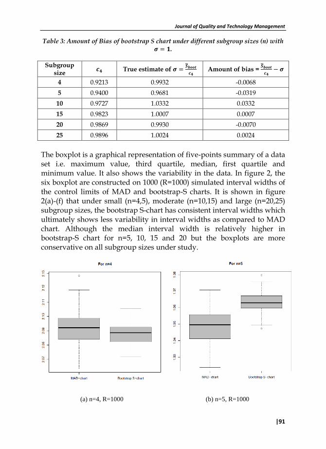
Table 3: Amount of Bias of bootstrap S chart under different subgroup sizes (n) with .

Subgroup size

True estimate of

Amount of bias =

4 0.9213 0.9932 -0.0068

5 0.9400 0.9681 -0.0319

10 0.9727 1.0332 0.0332

15 0.9823 1.0007 0.0007

20 0.9869 0.9930 -0.0070

25 0.9896 1.0024 0.0024

The boxplot is a graphical representation of five-points summary of a data set i.e. maximum value, third quartile, median, first quartile and minimum value. It also shows the variability in the data. In figure 2, the six boxplot are constructed on 1000 (R=1000) simulated interval widths of the control limits of MAD and bootstrap-S charts. It is shown in figure 2(a)-(f) that under small (n=4,5), moderate (n=10,15) and large (n=20,25) subgroup sizes, the bootstrap S-chart has consistent interval widths which ultimately shows less variability in interval widths as compared to MAD chart. Although the median interval width is relatively higher in bootstrap-S chart for n=5, 10, 15 and 20 but the boxplots are more conservative on all subgroup sizes under study.

(a) n=4, R=1000 (b) n=5, R=1000


92|

(c) n=10, R=1000 (d) n=15, R=1000

(e) n=20, R=1000 (f) n=25, R=1000

Figure 2: Boxplots of the 1000 simulated interval widths of the control limits of

MAD and bootstrap-S charts under different subgroup sizes (n).


|93

4.3) Example C: Piston Rings Data The practical data is considered from the standard text book of statistical quality control to illustrate the use of proposed control chart (see example 5-3, Montgomery, 2001). The inside diameter of the 25 piston rings (each of size 5) manufactured by this process is considered. To justify the findings of the simulation results, the control limits on practical data are being calculated in table 5. As the simulation results in the previous section showed that bootstrap S limits are very close to the exact limits of the process under normality condition so we can expect that they are more precise limits. For the piston ring data showed in table 4, the assumption of normality is confirmed by testing through Shapiro Wilk test of normality. The control limit of S and MAD are calculated by using eq. 4-6 & 7-9 while bootstrap S limits are constructed by using eq. 10-12 for which 1000 bootstrap samples are considered.

Table 4: Piston ring data for 25 samples

Sample No. Observations

1 74.030 74.002 74.019 73.992 74.008

2 73.995 73.992 74.001 74.011 74.004

3 73.988 74.024 74.021 74.005 74.002

4 74.002 73.996 73.993 74.015 74.009

5 73.992 74.007 74.015 73.989 74.014

6 74.009 73.994 73.997 73.985 73.993

7 73.995 74.006 73.994 74.000 74.005

8 73.985 74.003 73.993 74.015 73.988

9 74.008 73.995 74.009 74.005 74.004

10 73.998 74.000 73.990 74.007 73.995

11 73.994 73.998 73.994 73.995 73.990

12 74.004 74.000 74.007 74.000 73.996

13 73.983 74.002 73.998 73.997 74.012

14 74.006 73.967 73.994 74.000 73.984

15 74.012 74.014 73.998 73.999 74.007

16 74.000 73.984 74.005 73.998 73.996

17 73.994 74.012 73.986 74.005 74.007

18 74.006 74.010 74.018 74.003 74.000


94|

Sample No. Observations

19 73.984 74.002 74.003 74.005 73.997

20 74.000 74.010 74.013 74.020 74.003

21 74.982 74.001 74.015 74.005 73.996

22 74.004 73.999 73.990 74.006 74.009

23 74.010 73.989 73.990 74.009 74.014

24 74.015 74.008 73.993 74.000 74.010

25 73.982 73.984 73.995 74.017 74.013

The findings of the table 5 showed that MAD control limits are far beyond the S and bootstrap S limits. The advantage of bootstrap limits is that through these limits the original process standard deviation can be

calculated. The

is true estimator of which can easily be computed

by using

(where =0.9400). So we can expect the true process

standard deviation of the inside diameter of piston rings is 0.00999. Table 5: Calculation of S, MAD and bootstrap S control limits for piston ring data.

Control Chart Control limits

LCL CL UCL

S 0 0.0094 0.0196

MAD 0 0.01036 0.02164

Bootstrap S 0 0.00939 0.01961

5) CONCLUSION The control limits are same as confidence interval in hypothesis testing. Similar to the acceptance region in testing problems, we expect that the most precise control limits are those which can truly estimate the population parameter with smaller confidence width. Shawiesh (2008) proved that robust MAD estimator is still efficient under the normally distributed process because the control limits based on MAD estimator have more number of out of control points as compared to the Shewhart S chart. Our simulated results show that bootstrap S control chart has better performance as compared to the robust MAD chart under the assumption of normality. It is proved through simulations that the proposed chart has better in-control average run length, high coverage probability (close to the nominal value) and smaller expected


|95

interval width. The boxplot in figure 2 showed that bootstrap S chart will always exhibit precise interval width of containing original process standard deviation under different subgroup sizes. The precision of control intervals can also be ensured through the coverage probability close to the nominal value 0.9973 (as shown in table 2). The bootstrap S chart can also help in knowing true process standard deviation which is usually unknown in practice. A large number of bootstrap samples can provide unbiased estimator of process standard deviation. The results showed that under standard normal process the

mean of bootstrap

is true estimator of process standard deviation which

can easily be calculated by using the value of central line of bootstrap S

chart divided by . The simulation results of table 3 showed that

was

very close to the true value of process standard deviation from which the process was generated. Furthermore on the basis of smaller amount of bias, the most recommended subgroup size is 15. Under good theoretical properties of bootstrap methods, its application on the statistical process control is becoming popular. The future research can be carried out on the comparison of different bootstrap methods for the calculation of control limits. Furthermore these methods may have wide application in multivariate processes (Liu and Tang, 1996).

REFERENCES Efron, B., Tibshirani, R.J., (1993), An Introduction to the Bootstrap,

Chapman and Hall, Inc., New York, NY. Efron, B. (1979), “Bootstrap Methods: Another Look at the Jackknife”, The

Annals of Statistics. 7, 1-26. Grant, E.L. and Leaven-Worth, R.S. (1996) “Statistical Quality Control

Handbook” 7th edition, McGraw Hill Book Company, New York. Hampel F.R. (1974), “The influence curve and its role in robust

estimation”, J. Am. Stat. Assoc., 69: 383-393 Klein M. (2000), “Modified S-Charts for Controlling Process Variability”,

Communications in Statistics -Simulation and Computation, 29:3, 919-940.

Li H. Q, Tang M, Poon W.Y & Tang N. S. (2011), “Confidence Intervals for Difference between Two Poisson Rates”, Communications in Statistics - Simulation and Computation, 40:9, 1478-1493.


96|

Liu R. Y. (1995), “Control Charts for Multivariate Processes”, Journal of the American Statistical Association, 90(432), pp. 1380-1387.

Liu R.Y. and Tang. J. (1996), “Control Charts for Dependent and Independent Measurements Based on Bootstrap Methods”, Journal of the American Statistical Association (JASA), 91(436), pp. 1694-1700.

Liu Y, Liang J. and Qian J. (2004), “Moving Blocks Bootstrap Control Chart for Dependent Multivariate Data”, IEEE International Conference on Systems, Man and Cybernetics. pp: 5177-82.

Mills, J. D. (2002), “Using computer simulation methods to teach statistics: a review of the literature”, Journal of Statistics Education [Online], 10(1). www.amstat.org/publications/jse/v10n1/mills.html

Montgomery, D. C. (2001). Introduction to Statistical Quality Control. 4th ed. New York: John Wiley & Sons.

Niwitpong S. (2011), “Coverage Probability of Confidence Intervals for the Normal Mean and Variance with Restricted Parameter Space”, World Academy of Science, Engineering and Technology, 56

Rousseeuw, P.J. and C. Croux, (1993), “Alternatives to the Median Absolute Deviation”, J. Am. Stat. Assoc., 80: 1273-1283.

Shawiesh M. O. A. (2008), “A Simple Robust Control Chart based on MAD”, Journal of Mathematics and Statistics, 4(2), pp: 102-107.

Shewhart, W.A. (1931), “Economic Control of Quality of Manufacturing Product”,

New York: Van Nostrand. Simon, J. L., Atkinson, D. T., and Shevokas, C. (1976), “Probability and

statistics: experimental results of a radically different teaching method”, American Mathematical Monthly, 83(9), 733-739.

Stomberg A. J. (2001), “A New Nonparametric Control Chart for the Range”, Proceedings of the Annual Meeting of the American Statistical Association, August 5-9.

Wang H. (2009), “Exact Average Coverage Probabilities and Confidence Coefficients of Confidence Intervals for Discrete Distributions”, Communications in Statistics - Simulation and Computation, 19: 139–148.

Wood M. (2005), “The Role of Simulation Approaches in Statistics”, Journal of Statistics Education [Online], 13 (3).

www.amstat.org/publications/jse/v13n3/wood.html Yawsaeng B. & Mayureesawan T. (2012), “Control Charts for Zero-

Inflated Binomial Models”, Thailand Statistician, 10(1):107-120.

http://www.amstat.org/publications/jse/v10n1/mills.html

http://www.amstat.org/publications/jse/v13n3/wood.html

the bootstrap s-chart for process variability: an

Documents