the boltzmann–grad limit for a particle system in a slab with stochastic walls

*Correspondence to: S. Caprino, Dipartimento di Matematica, Universita di Roma Tor Vergata, Rome,Italy

CCC 0170—4214/98/171543—16$17.50 Received 4 September 1997( 1998 B. G. Teubner Stuttgart—John Wiley & Sons, Ltd.

Mathematical Methods in the Applied SciencesMath. Meth. Appl. Sci., 21, 1543—1558 (1998)MOS subject classification: 76 P 05; 82 A 40; 60 K 35

The Boltzmann—Grad Limit for a Particle System ina Slab with Stochastic Walls

S. Caprino1,* and B. Zavelani2

1 Dipartimento di Matematica, Universita di Roma Tor Vergata, Rome, Italy2 Dipartimento di Matematica, Uniersita di Trento, Italy

Communicated by H. Neunzert

It is shown that a stochastic system of N interacting particles in a slab approximates, in the Boltzmann—Grad limit, a one-dimensional Boltzmann equation with diffusive boundary conditions. ( 1998B. G. Teubner Stuttgart—John Wiley & Sons, Ltd.

1. Introduction

The Boltzmann equation represents the time evolution of the density for a rarefiedgas. The physical interpretation of this equation has been made rigorous since 1975for a short-time interval. More precisely, considering a suitable system of N interac-ting particles and looking at their joint distribution functions, it has been shown byLanford in Reference 5 that these functions factorize in the Boltzmann—Grad limit,provided they factorize at time zero, and that the limit one-particle distributionfunction satisfies the Boltzmann equation. It is difficult to extend this result to anarbitrarily fixed time interval, since, to know that the correlations among particlesdisappear in this limit, one has in principle to control the dynamics of the N particlesfor a long time and this is, in general, a very hard task. For a review on this problem,see Reference 4.

One possibility to approach this problem, which is also known as the ‘propagationof chaos’, is to deal with one-dimensional systems which, although unphysical, cankeep some of the important features of the general problem and moreover exhibita simpler dynamics.

In this paper, we approach a one-dimensional (in space and velocities) time-dependent Boltzmann-like equation in a slab, with diffusive boundary conditions. Weshow that this equation can be deduced from an N-particle system in the Boltzmann

Grad limit, that is letting NPR and eP0, holding the product eN finite, where e isthe collision probability for a given pair of particles. More precisely, we introducea density on the N-particle system and the relative j-particle distribution functions f N

jand we prove that they converge, in the above limit, to the j-fold product of thesolution of the Boltzmann equation.

This problem is a generalization of a similar one in Reference 2, in which a one-dimensional discrete velocities model Boltzmann equation on the whole line has beenrigorously derived. There the notion of ‘cluster’ of particles which influence a givenparticle has been introduced and some probability estimates which will be very usefulalso in the problem at hand has been proved. We want to mention also the paper [3]in which the cluster concept is applied to a stationary one-dimensional Boltzmannequation.

The general strategy used in Reference 2 to prove the result cannot be applied toour case for technical reasons, due to the fact that we have continuous velocities (seealso Reference 6 for related considerations). Thus, we combine the cluster techniquewith a crucial continuity property of f N

j(t) with respect to the initial datum, which is

proven in Proposition 3.2. Throughout the paper we assume that the solution to thelimit Boltzmann equation admits a ¸

=bound. The plausibility of such an assumption

is discussed in Remark 3.1. and in the appendix.As a final remark, we want to stress that we consider ‘logical’ clusters, independent

of the true dynamics. This technique on one hand allows us to prove the main resultswithout going into the details of the N-particles motion, but on the other hand is notsuitable for more realistic cases as three-dimensional velocities, as the definitions from4.4 and 4.7 would make no more sense.

The paper is organized into four sections. The N-particle model and all definitionsand notation used through the paper are introduced in section 2, while our maintheorems are stated and proved in section 3. All technicalities are left to section 4,devoted to the cluster technique and to the proof of some preliminary results.

2. The N-particle model

We consider a system of N point particles in the interval [0, 1]. Position andvelocity of the ith particle will be denoted by the couple of numbers (x

i, v

i) or,

equivalently, by zi"(x

i, v

i). Capital letters (X

N, »

N) (or Z

N) will stand as a shorthand

notation for the 2N-vector (x1, v

1, x

2, v

2, . . . , x

N, v

N). The phase space is

!N"([0, 1]]»)N,

where » is a compact set in R1, symmetric with respect to zero and we call A itsmaximum value. The particles are assumed to be indistinguishable and to follow thefree motion, unless two of them undergo a collision or one of them arrives at the walls,i.e. the points 0 and 1. We describe the two events:

(a) whenever a couple of particles i and j arrives at the position xi"x

jwith incoming

velocities such that sign vivj(0, then a pairwise collision takes place with prob-

ability e, while with probability 1!e they go ahead. The collision rule for the

1544 S. Caprino and B. Zavelani

Math. Meth. Appl. Sci., 21, 1543—1558 (1998)( 1998 B. G. Teubner Stuttgart—John Wiley & Sons, Ltd.

outgoing velocities (v@i, v@

j) is the following:

(v@i, v@

j)"(!v

j, !v

i), (2.1)

(b) when a particle arrives at the boundary of the interval [0, 1] it is stochasticallyreflected with an opposite sign velocity, distributed according to two boundedfunctions, M@

0:»WR`PR` and M@

1:»WR~PR`, relative to the points 0 and

1, respectively, and such that

P dv M@0

(v)"P dv M @1(v)"1.

This system can be interpreted as a model of a one-dimensional gas between twothermal reservoirs (placed at 0 and 1) at possibly different temperatures.

Remark 2.1. The collision rule described in (a) allows conservation of the kineticenergy and of the relative velocity, but these quantities are no more preserved in thepresence of stochastic boundaries. The collision law (2.1) has been defined in order tohave no recollisions between two particles in the time between two reflections of oneof them with the walls. This is only an apparent restriction since, the particles beingindistinguishable, we could equivalently have the pure reflection of the velocities.

We denote by ¹ tZN

the stochastic process described above at time t, starting almostsurely from Z

N. We will be more precise about its definition in section 4. Assume that

the particles are distributed at time zero according to a symmetric (in the exchange ofvariables) probability density kN, then the stochastic process ¹ tZ

Ninduces a time

evolution on kN in the following way. Calling kNt

the evolved measure at time t andsetting

kNt(Z

N) :"PN

tkN (Z

N), (2.2)

it is defined by

P dZNPN

tkN(Z

N) /(Z

N)"P dZ

NkN(Z

N)E [/ (¹ tZ

N)], (2.3)

where / is any smooth test function and E is the expectation with respect to theprocess. The density kN

tformally satisfies the following initial value problem (see

Reference 3):

At#N+i/1

vix

iB kNt(Z

N)"e +

i(j"1,2, N

d (xi!x

j) s (sign v

ivj(0),

D vi!v

jD [kN

t(Z@

N(i, j))!kN

t(Z

N)], (2.4)

kN0

(ZN)"kN (Z

N)

to which we must add the boundary conditions: for vi'0 (i"1,2, N)

kNt

(x1, v

1,2, 0, v

i,2 , x

N, v

N)

"M0(v

i) Pw

i(0

dwiDw

iD kN

t(x

1, v

1,2 , 0, w

i,2 , x

N, v

N) (2.5a)

Boltzmann—Grad Limit for a Particle System 1545


and for vi(0

kNt

(x1, v

1,2, 1, v

i,2 , x

N, v

N)

"M1(v

i) Pw

i'0

dwiwikNt

(x1, v

1,2, 1, w

i,2, x

N, v

N). (2.5b)

In (2.4) and (2.5) we make use of the following notation: d is the delta-function centredin 0 and s is the characteristic function of its argument. Moreover,

Z@N

(i, j)"(x1, v

1,2 ,x

i, v@

i,2,x

j, v@

j,2, x

N, v

N). (2.6)

M0

and M1

are defined by M@0

and M@1

in order to have the conservation of theprobability, which is a consequence of the property:

Pv'0

dv vM0(v)"Pv(0

dv D v D M1(v)"1. (2.7)

More precisely,

Ma (v)"M@a (v) CP dw Dw DM @a (w)D~1, a"0, 1.

(2.8)

From kNt

we can define the usual j-particle distribution functions, as

f Nj,t

(Zj)"P dz

j`1,2, dz

NkNt(Z

N)

which are, by definition, positive, symmetric, normalized and compatible. Integrating(2.4) we obtain for such functions the following hierarchy of equations, forj"1,2, N!1:

At#j+i/1

vix

iB f Nj,t

(Zj)"eG

jf Nj,t

(Zj)#e (N!j)C

j,j`1f Nj`1, t

(Zj), (2.9)

f Nj,0

(Zj)"f N

j(Z

j)

with the boundary conditions: for vi'0, i"1,2 , j

f Nj, t

(x1, v

1,2, 0, v

i,,2 ,x

j, v

j)

"M0

(vi) Pw

i(0

dwiD w

iD fN

j,t(x

1, v

1,2 , 0, w

i,2 ,x

j, v

j) (2.10)

and the analogous to (2.5.2) for vi(0 and x

i"1. The meaning of the symbols is the

following:

Gjf Nj,t

(Zj)" +

i(k"1,2, j

d (xi!x

k) s (sign v

ivk(0)

D vi!v

kD [ f N

j,t(Z@

j(i, k))!f N

j,t(Z

j)] (2.11)



and

Cj,j`1

f Nj`1,t

(Zj)" +

i"1,2, j P dvj`1

d (xi!x

j`1) s (sign v

ivj`1

(0)

D vi!v

j`1D [ f N

j`1,t(Z@

j`1(i, j#1))!f N

j`1, t(Z

j`1)]. (2.12)

Assume now that the f Nj,t

factorize, that is they are product of functions of a singlevariable, and perform the (formal) Boltzmann—Grad limit in (2.9), letting N go toinfinity and e to 0 in such a way that the product eN goes to j'0. Then, theone-particle distribution function satisfies the following model-Boltzmann initial-boundary value problem:

(t#v

x) g (x, v, t)"jQ (g, g) (x, v, t) (2.13)

g (x, v, 0)"g0

(x, v)

P dx dv g (x, v, t)"1

with boundary conditions for v'0

g (0, v, t)"M0(v) Pw(0

dw Dw Dg (0, w, t) (2.14a)

and for v(0

g (1, v, t)"M1(v) Pw'0

dw wg (1, w, t) (2.14b)

where, taking into account (2.1),

Q (g, g) (x, v, t)"P dv1s (vv

1(0) D v!v

1D [g (x,!v

1, t) g (x, !v, t)

!g (x, v, t) g (x, v1, t)] (2.15)

In fact, we are not allowed to make such a factorization assumption at the level of theN-particle gas, since, also if it is satisfied at time zero, the dynamics itself createcorrelations among particles. What can be actually proven, and we will do it in thenext section, is that the factorization property holds at later times t*0 after per-forming the Boltzmann—Grad limit on the N-particle system. The existence anduniqueness of the solution to (2.13) and (2.14), belonging to ¸

=([0, ¹ ], ¸`

1) has been

proven in Reference 1 in a more general case with unbounded velocities.

3. The main result

In what follows, Ci, i"0,1,2,2, denote positive constants, in general depending

upon the data of the problem (the wall functions M0

and M1, the maximum value of

the velocities A, etc.). In case some constant depends upon other relevant quantities,this will be explicitly written.



We put:

S f, gT"P dz f (z)g (z),

The main results of this paper are stated in the following two theorems.

Theorem 3.1. ¸et ¹'0 be arbitrarily fixed. Choose the solution to (2.13) and (2.14)such that E g

0E¸

=(#R and assume that there exists a positive constant C

0,

depending on ¹ and g0

such that

sup0)t)¹

E g (t) E¸=)C

0. (3.1)

¹hen, there exists j0'0 such that, if j)j

0, we can find a positive constant C

1such

that, if

f Nj,0

(Zj)"

j<i/1

g0(z

i),

then:

sup0)t)¹

E f Nj,t!

j<i/1

g (t) E¸

1)

Cj1

N. (3.2)

Theorem 3.2. In the same hypotheses of ¹heorem 3.1, for any positive j, we have

limNPR

sup0)t)¹

S f Nj,t

, ujT"T

j<i/1

g (t), ujU (3.3.)

for any bounded continuous function uj:!jPR`.

Remark 3.1. Assumption (3.1) on g (t) is satisfied in case we consider a suitable cutoffsystem, as it will be shown in the appendix. Unfortunately, we did not succeed inproving it, in general, since we have no control of the collisions with incomingvelocities, v

iand v

ksuch that the quantity D v

i#v

kD is arbitrarily small.

Remark 3.2. We think that the weaker convergence of Theorem 3.2 is only due totechnical reasons and can be strenghtened to the ¸

1-convergence, as discussed in

Reference 2.

The proof of Theorem 3.1 is based on two Propositions.

Proposition 3.1. ¹here exist positive constants, Ci, i"2, 3, 4 such that, if

jq E g0E¸=)C

2exp M!C

3qN (3.4)



for some positive time q and

f Nj,0

(Zj)"

j<i/1

g0(z

i),

then

sup0)t)q

E f Nj(t)!

j<i/1

g (t) E¸

1)

Cj4

N.

Let us denote by lN the probability density defined as

lN(ZN, t)"

N<i/1

g (zi, t)

and let us set

*N(ZN, t)"kN (Z

N, t)!lN (Z

N, t),

*Nj(Z

j, t)"f N

j(Z

N, t)!

j<i/1

g (zi, t). (3.5)

We have the following result:

Proposition 3.2. ¹here exists a positive constant C5

such that for any ¹'0 and anyt3[0, ¹ ], we have

P dZjD P dZ

N~jPN

t*N(Z

N, 0) D)ej +

s*0

E*Nj`s

(0) E¸1(C

5rj)s#OA

1

NBwith r"[2A¹#2].

The proof of Proposition 3.1 can be found in Reference 3. It consists in extending theclassical Lanford result of convergence for short time (see Reference 5) to the presentcase. The different ingredients in the proof are due to the presence of the stochasticwalls. Indeed, while the ¸

1-norm is still preserved in this case, this is not so for the

¸=-norm, in which the collision operator is naturally estimated.Proposition 3.2 is proven in section 4, where the main definitions and properties

concerning the clusters are also given.Propositions 3.1 and 3.2, together with Assumption 3.1, allow us to prove Theorem

3.1 via an inductive procedure on the time.

Proof of ¹heorem 3.1. Let q be such that

jqC0)C

2exp M!C

3qN (3.6)

and ¹'0 such that ¹"nq, for some integer number n. Notice that for n"1 thetheorem is proven by Proposition 3.1, thus the proof will proceed by induction.



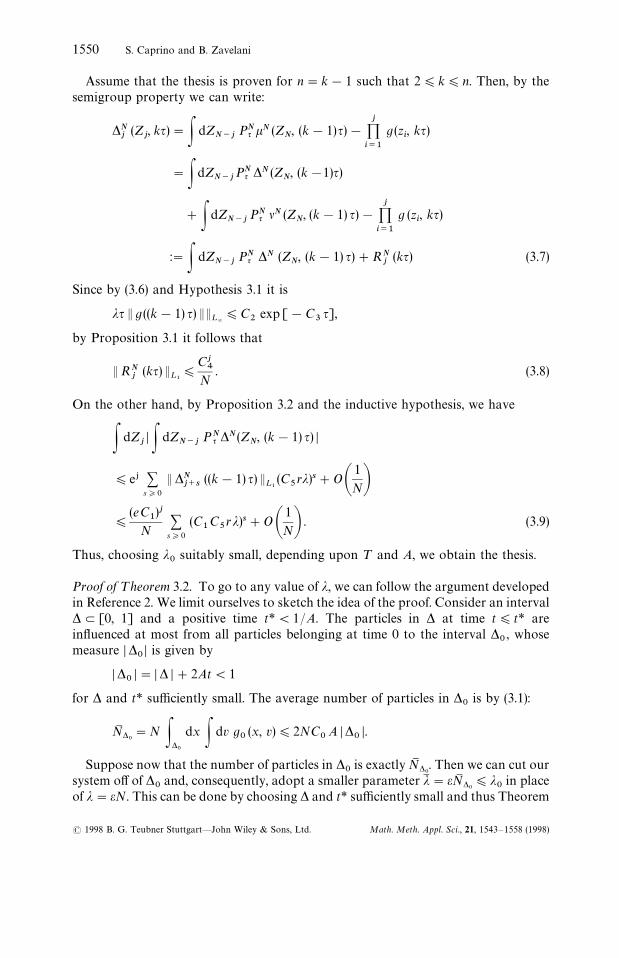
Assume that the thesis is proven for n"k!1 such that 2)k)n. Then, by thesemigroup property we can write:

*Nj

(Zj, kq)"P dZ

N~jPNq kN (Z

N, (k!1)q)!

j<i/1

g (zi, kq)

"P dZN~j

PNq *N (ZN, (k!1)q)

#P dZN~j

PNq lN (ZN, (k!1) q)!

j<i/1

g (zi, kq)

:"P dZN~j

PNq *N (ZN, (k!1) q)#RN

j(kq) (3.7)

Since by (3.6) and Hypothesis 3.1 it is

jq E g ((k!1) q) EE¸=)C

2exp [!C

3q],

by Proposition 3.1 it follows that

ERNj

(kq)E¸

1)

Cj4

N. (3.8)

On the other hand, by Proposition 3.2 and the inductive hypothesis, we have

P dZjD P dZ

N~jPNq *N(Z

N, (k!1) q) D

)e+ +s*0

E*Nj`s

((k!1) q) E¸

1(C

5rj)s#OA

1

NB)

(eC1)j

N+

s*0

(C1C

5rj)s#OA

1

NB . (3.9)

Thus, choosing j0

suitably small, depending upon ¹ and A, we obtain the thesis.

Proof of ¹heorem 3.2. To go to any value of j, we can follow the argument developedin Reference 2. We limit ourselves to sketch the idea of the proof. Consider an interval*L[0, 1] and a positive time t*(1/A. The particles in * at time t)t* areinfluenced at most from all particles belonging at time 0 to the interval *

0, whose

measure D *0D is given by

D *0D"D * D#2At(1

for * and t* sufficiently small. The average number of particles in *0

is by (3.1):

NM *0"N P*

0

dx P dv g0(x, v))2NC

0A D *

0D.

Suppose now that the number of particles in *0

is exactly NM *0. Then we can cut our

system off of *0

and, consequently, adopt a smaller parameter j1 "eNM *0)j

0in place

of j"eN. This can be done by choosing * and t* sufficiently small and thus Theorem



3.1. holds, restricting ourselves to the region *0. This implies the same result over the

whole of [0, 1] and finally the uniform bound (3.1) allows us to go to further time 2t*and so on, up to the fixed time ¹. This argument implies that, in order to prove thetheorem, we are reduced to control the fluctuations of the number of particles ina given region *

0at time 0, with respect to its average number. Actually, this has been

done in Reference 2 and can be adapted to the present case, with minor modificationsdue to the presence of the stochastic walls. Thus, we omit the proof here.

4. The cluster technique

To prove Proposition 3.2., we start by giving a representation of the stochasticprocess ¹ t Z

N, already introduced in section 2, in a suitable sample space, that is

)"M0, 1N[rN (N!1)]/2 (4.1)

for r3Z`. Any u3) is a function of three integers such that: u (i, j; a)"u( j, i; a) fori9j, taking values 0 or 1, for a"0, 1,2, r. The integers i and j represent a couple ofcolliding particles, while a is the number of recollisions they undergo due to thepresence of the walls (we recall, as we said in Remark 2.1, that the dynamics do notallow any other kind of recollision). For a fixed u we can define the following processwhose only stochasticity comes from the stochastic boundaries:

¹ tu : ZN3!NP¹ tuZN3!N.

The process ¹ tu is the Knudsen flow (that is free motion with stochastic boundaryconditions) up to the time in which two particles i and j arrive at the same site withopposite sign velocities. Then, if they have already met a!1 times and u (i, j; a)"1,they collide with the collision rule given in (2.1), otherwise they keep following theKnudsen flow. Notice that, the velocities being bounded, two particles can meet atmost k times, with k)2At#2 in the time interval [0, t], so that, for a fixed ¹'0, it is

r)2A¹#2. (4.2)

We define the probability of u as

p (u)"<1(j

r<a/1

eu(i, j; a) (1!e)1!u (i, j; a). (4.3)

Then M), pN is a probability space and the expectation in (2.3) has to be intended as

E [/ (¹ t ZN)]"E) E

B[/ (¹ tu Z

N)]

EB

being the expectation with respect to the outgoing distribution of the velocities atthe boundary (recall (2.5)) and Eu the expectation with respect to M), pN.

Note that the stochastic process we have described is not a Markov process, since todefine it at time t one has to know what happened at previous times.

Now, we give the definition of cluster, which is of great importance in our setup. LetIM"M1, 2,2 ,MN and let I indicate any set of indices. Given u3) we call ‘chain’



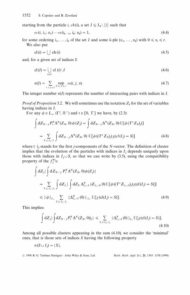
starting from the particle i, ch (i), a set I-INCMiN such that

u (i, i1; a

1)2u (i

k~1, i

k; a

k)"1, (4.4)

for some ordering i1,2 , i

kof the set I and some k-ple (a

1,2, a

k) with 0)a

i)r.

We also put

cl (i)"Z ch (i) (4.5)

and, for a given set of indices I:

cl (I)"Zi|I

cl (i)CI (4.6)

n(I)" +i(j3I

sup0)a)r

u (i, j, a). (4.7)

The integer number n(I) represents the number of interacting pairs with indices in I.

Proof of Proposition 3.2. We will sometimes use the notation ZIfor the set of variables

having indices in I.For any /3¸

=(!j, R`) and t3[0, ¹] we have, by (2.3):

P dZN~j

PNt*N (Z

N, 0)/ (Z

j)"P dZ

N~j*N (Z

N, 0)E [/ (¹ tZ

N)j)]

" +S-I

NCI P dZ

N~j*N (Z

N, 0) E [/ ((¹ tZ

N)j)s(cl (I

j)"S)] (4.8)

where ( ) )jstands for the first j-components of the N-vector. The definition of cluster

implies that the evolution of the particles with indices in Ijdepends uniquely upon

those with indices in IjXS, so that we can write by (3.5), using the compatibility

property of the f Nj’s:

P dZjD P dZ

N~jPN

t*N (Z

N, 0)/ (Z

j) D

" +S-I

NCI

jP dZI

jD P dZ

S*NI

jXS (ZI

jXS, 0)E [/ ((¹ tZI

jXS)j

)s (cl (Ij)"S)]D

)E/E¸=

+S-I

NCI

j

E*NIjXS (0) E

¸1E [s (cl(I

j)"S)]. (4.9)

This implies:

P dZjD PdZ

N~jPNt

*N (ZN, 0))

jD) +

S-INCI

j

E*NIjXS (0) E

¸1E [s (cl (I

j)"S )].

(4.10)

Among all possible clusters appearing in the sum (4.10), we consider the ‘minimal’ones, that is those sets of indices S having the following property

n (SX Ij)"D S D,



where D S D is the number of indices in S. This means that the number of links amongthe particles in SXI

jis the least for the cluster to be settled. Putting S

i"cl (i) for i3I

j,

we see that in this case it is ShWS

k"0 if h9k. Thus, equation (4.10) is

) +S-I

NCI

j

E*IjXS (0) E

¸1,

G*+

S1,2 ,S

j

E Cj

<i/1

s (cl(i)"Si)s (n (SM

i) "DS

iD )D

#E[s (cl (Ij)"S )s (n (I

jXS)'D S D ]H (4.11)

where +* stands for the sum over mutually disjoint sets S1,2 ,S

jsuch that XS

i"S

and SMi"S

iXMiN. We call p

1and p

2the first and second term in (4.11) respectively. The

main estimates to prove this proposition can be deduced in analogy with the case ofa particle system on the whole line (see Section 5 in Reference 2). The probability tohave u (i, j; a)"1 (see (4.7)) for some a, for the pair (i, j), is bounded by re. Moreover,the number of ways we have to arrange a cluster S

iaround the ith particle is bounded

by DSiD !CDS

iD

6. Hence,

p1) +

S-INCI

j

E*IjXS (0) E

¸1

*+

S1,2,S

j

j<i/1

DSiD ! (C

6re)DSi

D

) +S-I

NCI

j

E *IjXS (0) E

¸1

*+

s1,2 , s

jA

s

s1B A

s!s1

s2B2 A

s!+j~1i/1

sj

siB

j<i/1

si! (C

6re)si

(4.12)

with s, siin place of D S D, D S

iD. Recalling now that eNPj and noticing that

*+

s1,2, s

j

1)es`j , AN

s Bs!

Ns)1,

we obtain after a few calculations

p1)ej +

s*0

E*Nj`s

(0) E¸1(C

6rj)s. (4.13)

For the second term, we have the following estimate:

p2"O A

1

NB . (4.14)

Formula (4.14) tells us that the event for a set of tagged particles to have not a minimalcluster, is a rare one. This is due to the fact that more collisions among particles bringinto the game more small factors of order j/N, and can be proven by adapting to thiscontext the analogous result given in Section 5 of Reference 2. This completes theproof.



Appendix

Consider the following boundary value problem:

(t#v

x) f (x, v, t)"QM (x, v, t),

f (x, v, 0)"f0

(x, v),

f (0, v, t)"M0(v) Pw(0

dw D w D f (0, w, t)

for v'0, while for v(0:

f (1, v, t)"M1

(v) Pw'0

dw w f (1, w, t) (A1)

with

QM (x, v, t)"P dv1s (vv

1(0)s( D v#v

1D*a),

[ f (x,!v1, t) f (x,!v, t)!f (x, v

1, t) f (x, v, t)]. (A2)

This system preserves the ¸1

norm of the solution. We assume for technical reasons(see (A.18)) that

supv

log Ma (v)(#R a"0, 1.

Defining the usual entropy:

H (t)"P dx dv f (x, v, t) log f (x, v, t),

we have the following result.

Theorem A1. Assume that H (0) is finite. ¹hen, for any ¹'0 there exists a constantC

0depending on ¹ and H (0) such that

sup0)t)¹

E f (t) E¸=)C

0E f

0E¸

=.

Proof. First of all write problem (A1) in a mild form. Setting for v'0

b (x, v, t)"max G0, t!x

vHand for v(0

B (x, v, t)"maxG0, t!1!x

D v D H



we have for v'0:

f (x, v, t)"f0

(x!vt, v) s (x!vt'0)#f A0, v, t!x

vBs (x!vt)0)

#Pt

b (x, v,t)

dsQM (x!v (t!s), v, s) (A3)

and for v(0:

f (x, v, t)"f0

(x!vt, v) s (x!vt(1)#f A1, v, t!1!x

D v D Bs (x!vt*1)

#Pt

B (x, v,t)

dsQM (x!v (t!s), v, s). (A4)

Passing to the d-formalism, that is defining

f d(x, v, t)"f (x#vt, v, t)

for any (x, v, t) such that x#vt3[0, 1], we obtain for v'0

f d(x, v, t)"f0(x, v)s (x'0)#f A0, v,

!x

v B s (x)0)

#Pt

bd (x, v,t)

ds QM d (x, v, s), (A5)

while, for v(0,

f d (x, v, t)"f0(x, v)s(x'1)#f A1, v,

1!x

D v D B s (x*1)

#Pt

Bd (x, v,t)

ds Qd (x, v, s), (A6)

where, setting

h (v, v1)"s (vv

1)0)s ( D v#v

1D*a),

it is

QM d (x, v, s)"P dv1D v!v

1D h (v, v

1) f d (x#(v#v

1)s,!v

1, s) f d (x#2vs,!v, s)

!f d (x, v, s) f d Yx#(v!v1)s, v

1, s)]. (A7)

Let t0

be a positive time. We have for any s)t0:

DQM d(x, v, s) D

)2 sup0)s)t

0

E f (s) E¸

= P dv1D v#v

1D h (v,!v

1) D f (x#(v!v

1) s, v

1, s) D (A8)



and, after a suitable change of variables,

Pt0

0

ds D Qd(x, v, s) D)4A

asup

0)s)t0

E f (s) E¸

=DDD f DDDt

0, (A9)

where

DDD f DDDt0"P dxdv sup

0)s)t0

D f d (x, v, s) D. (A10)

Choose now t0)1/A. Then, (2.14) and (A6) imply that for v'0:

f A0, v,!x

v Bs (x)0)"s(x)0)M0(v) P

w:0

dw Dw D f A0, w,!x

v B"s (x)0) M

0(v) P

w:0

dw D w DG f0 A

wx

v, wB#P

~x @v

0

ds Qd Awx

v, w, sBH .

(A11)

Indeed, t0

has been chosen small enough to guarantee that there is at most onecollision with the walls, (that is B (x, v, t)"0 in (A3)). Thus, by (A10) and (A11) wehave, for v'0:

D f A0, v,!x

v B)C7

[E f0E¸=#DDD f DDD t

0sup

0)t)t0

E f (t) E¸=] (A12)

with C7

depending uniquely on the data of the problem. We can proceed analogouslyfor v(0 so that, going back to (A5), (A6) and (A9) we may write:

sup0)t)t

0

E f (t) E¸=)C

8[ E f

0E¸=#DDD f DDDt

0sup

0)t)t0

E f (t) E¸=] . (A13)

In [1] it is shown that, if E f0E¸

1is smaller than a numerical constant, then

DDD f DDDt0)4E f

0E¸1. (A14)

Thus,

sup0)t)t

0

E f (t) E¸=)C

9E f

0E¸=

(A15)

provided that E f0E¸1is sufficiently small.

Now, the basic ingredient to go to any initial datum is a bound on the entropy,which in this setup is no more decreasing, for the presence of the stochastic walls.Nevertheless, we can easily find such a bound, because the velocities are in a compactset. Proceeding by the usual computations, we arrive at

H (t)!H (0))Pt

0

ds P dv v [ f log f (0, v, s)!f log f (1, v, s)]. (A16)



The following inequalities can be found, for instance, in Reference 4:

P dv vf logf

M0

(0, v, s))0, (A17.1)

P dv vf logf

M1

(1, v, s)*0, (A17.2)

and these imply that

H(t))H (0)#C10 P

t

0

ds [J (0, s)#J (1, s)], (A18)

where

J (a, s)"P dv D v D f (a, v, s), a"0, 1 (A19)

and C10

is a constant depending on the data of the problem. Moreover, the ratherobvious estimate (proven in Reference 1):

Pt0

0

ds J(a, s))E f0E¸1

(A20)

implies for any t3[0, ¹]

Pt

0

ds J (a, s))C11

E f0E¸1

(A21)

with C11

proportional to A¹. Hence (A18) and (A21) allow to prove the searchedbound:

H(t))H(0)#C12

(¹, E f0E¸1). (A22)

The above estimate imply that (A15) holds for any initial condition up to any fixedtime interval [0, ¹ ]. The argument is of the same kind as that in the proof of Theorem3.2. More precisely, the solution f (t) to problem (A1) is known for t3[0, t*] andx3*, a subinterval of [0, 1], once it is known at time zero over a bigger interval *

0.

The measure of *0

can be made small, by choosing t* and * small, and E f0D*

0E¸1can

be made as small as we want, by the finiteness of H (0) ( f0D *

0is the restriction of f

0to

*0). Thus, (A15) can be proven for f (t) D * , starting from any initial datum, for a short

time t*. Finally, the bound (A22) allows to go to further time 2t* and so on, up totime ¹.

References

1. Caprino,. S., ‘The initial value problem for a one-dimensional Boltzmann equation with diffusiveboundary conditions’, Rendiconti di Matematica, serie VII, vol. 17, Roma (1997).



2. Caprino, S. and Pulvirenti, M., ‘A cluster expansion approach to a one-dimensional Boltzmannequation: a validity result, Comm. Math. Phys. 166 (1995).

3. Caprino, S. and Pulvirenti, M., ‘The Boltzmann-Grad limit for a one-dimensional Boltzmann equationin a stationary state, Comm. Math. Phys. 177 (1996).

4. Cercignani, C., Illner, R. and Pulvirenti, M., ¹he Mathematical ¹heories of Diluite Gases, Springer seriesin Appl. Math, 106, 1994.

5. Lanford, O. III, Lect. Notes in Physics, 35, Springer, New York 1975.6. Pulvirenti, M. Lect. Notes in Mathe., Springer, 1627, 1995.



the boltzmann–grad limit for a particle system in a slab with stochastic walls

Documents