the binomial model in fluctuation analysis of quantal ... · arise in n' (reduced cvp) tends...
TRANSCRIPT
Biophysical Journal Volume 72 February 1997 728-753
The Binomial Model in Fluctuation Analysis of QuantalNeurotransmitter Release
D. M. J. QuastelDepartment of Pharmacology and Therapeutics, Faculty of Medicine, The University of British Columbia, Vancouver, British ColumbiaV6T 1Z3 Canada
ABSTRACT The mathematics of the binomial model for quantal neurotransmitter release is considered in general terms, toexplore what information might be extractable from statistical aspects of data. For an array of N statistically independentrelease sites, each with a release probability p, the compound binomial always pertains, with (m) = N(p), p' 1 - var(m)/(m)- (p) (1 + cvp) and n' (m)/p' = N/(1 + cvp), where m is the output/stimulus and cvp is var(p)/(p)2. Unless n' is invariantwith ambient conditions or stimulation paradigms, the simple binomial (cvp = 0) is untenable and n' is neither N nor thenumber of "active" sites or sites with a quantum available. At each site p = PaPA' where po is the output probability if a siteis "eligible" or "filled" despite previous quantal discharge, and PA (eligibility probability) depends at least on the replenishmentrate, po, and interstimulus time. Assuming stochastic replenishment, a simple algorithm allows calculation of the full statisticalcomposition of outputs for any hypothetical combinations of p,'s and refill rates, for any stimulation paradigm andspontaneous release. A rise in n' (reduced cvp) tends to occur whenever po varies widely between sites, with a raisedstimulation frequency or factors tending to increase po's. Unlike (m) and var(m) at equilibrium, output changes early in trainsof stimuli, and covariances, potentially provide information about whether changes in (m) reflect change in (po) or in (PA)-Formulae are derived for variance and third moments of postsynaptic responses, which depend on the quantal mix in thesignals. A new, easily computed function, the area product, gives noise-unbiased variance of a series of synaptic signals andits peristimulus time distribution, which is modified by the unit channel composition of quantal responses and if the signalsreflect mixed responses from synapses with different quantal time course.
INTRODUCTION
From the first description of the quantal nature of neuro-transmitter release and its probabilistic character it has beengenerally assumed that the distribution of numbers ofquanta released by stimuli is in some sense binomial incharacter, with a Poisson distribution appearing under con-ditions of depressed release (low Ca2+/raised Mg2+), so thateach stimulus effectively samples with low probability froma relatively large number of release sites (del Castillo andKatz, 1954a; Martin, 1955). Since then many studies of avariety of synapses have found deviations from a Poissondistribution in the direction expected with a binomial dis-tribution (rev. McLachlan, 1978; Redman, 1990).A binomial distribution for outputs corresponds to the a
priori consideration that the number of quanta released by astimulus must be limited by the number of release sites andthe number of quanta available for release. Equally a priori,however, there is no reason to assume that the probability ofrelease is the same for every site and that this probability isthe same from one stimulus to the next, which are bothpreconditions for a simple binomial distribution of outputsfor which the mean ((m)) is np and the variance, var(m), isnp(l - p), where n is the number sampled with probability p.
Received for publication 25 September 1995 and in final form 1 October1996.Address reprint requests to Dr. D. M. J. Quastel, Department of Pharmacologyand Therapeutics, Faculty of Medicine, The University of British Columbia,2176 Health Sciences Mall, Vancouver BC V6T 1Z3, Canada. Tel.: 604-822-4263; Fax: 604-822-6012; E-mail: [email protected].© 1997 by the Biophysical Society0006-3495/97/021728/26 $2.00
The case in which p and n may vary spatially and tem-porally was considered by Brown et al. (1976), who showedthat the p and n obtained from data assuming a simplebinomial (i.e., p' = 1 - var(m)/(m) and n' = (m)lp') thenbear no relation to the true mean p ((p) ) and the true (mean)number of sites capable of release, except that n', like thenumber of "filled" or "eligible" sites, must be less than thetotal number of sites, and p', like any p, must be ' 1. Giventhat at each release site p must be the product of outputprobability (po) and the probability that the site is "eligible"(PA), the simple binomial (all release sites equivalent)should give n' always equal to the total number of releasesites. Numerous findings that n' varies with stimulationfrequency and ambient Ca2+/Mg2+ (see McLachlan, 1978)therefore indicate that the simple binomial does not applygenerally. Nevertheless, it is still common to find in the liter-ature the assumption that n' somehow represents the number ofrelease sites that have a quantum available for release.
It is my purpose here to consider the binomial model withminimal artificial constraints, emphasizing the underlyingassumptions and the way in which these translate mathe-matically into the consequent statistical properties of out-
puts and resulting postsynaptic signals. A synapse or groupof synapses is (conventionally) envisaged as an array of Nindependent release sites, each potentially capable of releas-ing only one quantum at a time, and each with its own p.Unless all release sites have the same p, giving the simplebinomial model, this is the compound binomial model (rev.McLachlan, 1978; rev. Redman, 1990; Dityatev, Kozhanovand Gapanovich, 1992), for which (m) is N(p), p' = (p)
728

Binomial Transmitter Release
(1 + cvp) and n' = N/(1 + cvp), where cvp is the coefficientof variation of p (Brown et al., 1976). It is shown that apartfrom the simplifying assumption that stimulated releaseoccurs over an infinitely brief time, the only necessaryassumption for this is site independence, which is also aprecondition for the simple binomial. Notably, if N is en-larged by any number, corresponding to hypothetical siteswith p -0, the above relationships remain true, with (p)and cv2 having new values; neither mean nor variance (oroverall distribution) of the outputs contains informationabout the number of release sites, unless the distribution ofp among these sites is known. One such distribution, namelythat p is the same at all "active" sites and 0 elsewhere, givesn' equal to the number of active sites, but is logicallyuntenable (see Discussion).One basic assumption of the binomial model, that release
by a stimulus is limited to a fixed maximum, is reconcilablewith reality (a noninfinitesimal time period of release) onlyif the release of a quantum by a site somehow entails thetemporary inability to release another. As the converse ofrelease, this "depletion" is inherently stochastic, and ifsubsequent "refilling" is also stochastic, events at each siteconstitute a Markov chain, corresponding to one of themodels considered by Vere-Jones (1966) and more recentlyby Melkonian (1993). Here I have generalized this model intwo ways, to the situation in which release sites havedifferent output probabilities (po's) and refill rates, and towhere these parameters vary in time, to make it possible tocompute statistical outcomes for any hypothetical parametersets and stimulus sequences, and for spontaneous release.One result that emerges is that ifpo varies between sites, cvpand the relative contribution of quanta from different sitescan be expected to change continually early in trains ofstimuli, to vary with stimulation frequency, and to vary withconditions that modify po's or the rate of refilling; n' tendsto rise with stimulation frequency and with any factor thatincreases po's.
I also present derivations of equations for the third mo-ment of the quantal outputs, for the modification of mo-ments by quantal amplitude variation of various types(Walmsley, 1993), and for the expected covariance betweennumbers of quanta released by successive stimuli, which,unlike means and variance, may contain information aboutwhether any experimentally observed changes in (p) or cvpmight be due to changes in p0's or PA'S (Vere-Jones, 1966).Statistical measures are also derived for "spontaneous" release.
In addition, a new function, the area product, is intro-duced; this is easily computed from data and provides notonly the total variance of sequential synaptic signals, unbi-ased by recording noise, but also the distribution in time ofthis variance before and after the point of stimulation. Withsome caveats, the latter can be an indicator of whether thesignals represent a mix from different synapses producingquantal responses of different time course, and/or providean estimate of the amplitude of the channels underlying
METHODS
All of the equations presented were derived from basicprinciples using approaches found in an introductory text-book of mathematical statistics (Weatherburn, 1961) and inVere-Jones (1966). Various calculations were done on anIBM-compatible PC, either with a spreadsheet or with pro-grams written in C. These calculations were of two kinds: 1)verification with a Monte Carlo simulation of the formulaefor variances and covariances and 2) determination of theeffect of arbitrarily assigned release probabilities and re-plenishment rates for arrays of up to 100 release sites inwhich one or both of these parameters varied between sites.Some of the results of these calculations are presented in theillustrative figures in the next section. In the simulations Iused, the ran2( subroutine of Press et al. (1992), which waschecked to verify the absence of correlations between suc-cessive pseudorandom numbers, to obtain random numbersbetween 0 and 1, from which, when required, exponentiallydistributed random numbers could be obtained by taking thenegative of the logarithm. For normally distributed randomnumbers I used the gasdev( subroutine of Press et al.(1992).
THEORY AND RESULTS
The simple and compound binomial distribution
Consider a synapse that has been stimulated repetitively ata constant rate, the outputs of which have settled down to avalue that is constant except for statistical fluctuations. Toobtain the statistical composition of the outputs (i.e., mean,variance, etc.) imagine records from a very large array ofdetectors that cover the whole presynaptic area. Each de-tector has as its territory an area so small that no more thanone quantum can be released in the (supposedly) infinitelybrief time period, after each stimulus, that release occurs; itsignals a 1 for a "success" and a 0 for a "failure." Becausethe number of detectors is much larger than the number ofrelease sites, the record from most of the detectors containsonly 0's, but others contain I's and 0's. For any one of theseactive sites there will be a certain number of l's, say s, fork stimuli. The sum over the k stimuli is s, the sum of squaresis s, and the sum of cubes is s. The mean = = meansquare = ,u' = mean cube = 3= s/k, for which theexpected value is p, the probability of release. Thus theexpected value of the mean = p and the second and thirdmoments about the mean are variance = p(l - p), thirdmoment = p - 3p2 + 2p3 = p(l - p)(l - 2p), i.e., outputsfrom each active site are binomially distributed with param-eters 1 and p.
In nearly all experimental situations the data we have foreach stimulus will correspond to the sum of the outputsfrom the hypothetical detectors. The mean and variance(and third moment) of these are obtained simply by sum-mation if and only if the numbers from each are uncorre-
quantal responses.
729Quastel
lated, i.e., whether or not a success occurs at any one

Biophysical Journal
detector is uncorrelated with whether or not a success oc-curs at any others. In other words, release sites must beindependent. Then,
E(m)= E p; var(m) = Ip- 2,p2
p' - var(m)/E(m) = E p2/lp
'E(i)/p' = (I p)2/ p2.
In terms of N, the number of release sites,
E(m) = N > p/N = N(p) (la)
var(m) = N(p) - N((p)2 + var(p))
= N(p)(l- (p)(l + var(p)/(p)2))
= N(p)(I - (p)(l + cvp)) (lb)
and
P' = (p)(l + cv2) (Ic)
n' = N/(1 + cvp2). (Id)
This is the "compound binomial." Note that Eqns. 1 arevalid for any assumed value of N 2 n' (because CV2 2);the mean and variance of outputs can give true N only if cvPis known a priori, or give true cvp only if true N is knowna priori. For one particular distribution of p, where p is thesame at all active sites and zero elsewhere, the situation isthe same as if the silent sites did not exist and in a sense thesimple binomial (cvp = 0) pertains; n' is the number ofactive sites, invariant with any alteration of p as long ascvp = 0, but true N remains unknown. Indeed, we could notdetermine true N even if we had access to the records fromeach and every detector, because a record with no successesdoes not preclude a past or future success.
It must be emphasized that if sites are not independent,Eqns. 1 do not pertain, even for cvp = 0, which is otherwisethe simple binomial (Brown et al., 1976).
Comparison of output distributions for simple andcompound binomials
The third moment of the outputs is given by
M3 = >p - 3Ep2 + 2Ep3= N(p) - 3N[(p)2 + var(p)]
+ 2N[(p)3 + 3(p) var(p) + P3]
= N[(p)(l - (p))(l - 2(p))
- 3 var(p)(l - 2(p)) + 2P3] (le)
where M3 and P3 denote the third moments of m and pabout their means. In general M3 is not the same for a
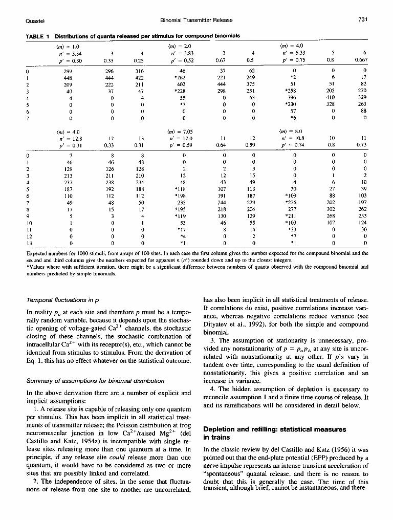
compound binomial as for the simple binomial, and it mighttherefore be supposed that from the output distribution onecould detennine whether a simple or a compound binomialpertains. However, simulations of outputs for a compoundbinomial show that this is not the case (Brown et al., 1976).The examples in Table 1 are for arrays of 100 sites witharbitrary widely varying p. In each case the first column isa list of the number of outputs with 0, 1, 2, etc. quantaexpected for 1000 iterations. The second and third columnsare calculated using the mean ((m)) and variance of theoutputs to obtain p' and n', rounding off n' down and up tointegers and choosing for each a new p' = (m)/(new) n'. Forexample, in the first set, certain parameters producing (m) =1 gave p' = 0.30 and n' = 3.34; the two simple binomialsfor comparison have n = 3 andp = 0.33 and n = 4 andp =0.25. The true distribution is either between the two forsimple binomials, or different from an extreme of the latterby no more than 4, i.e., not statistically significant; the samewas true for any set of p's giving about 30% or more"failures." Apart from the appearance of a few outputs morethan n', appreciable differences between the compoundbinomial and the corresponding simple binomials occuronly ifp' is more than about 0.5 and (m) is so high that thereare no failures and few if any unitary responses. The cor-ollary is that whereas an output distribution may sometimesshow that a simple binomial does not pertain, the absence ofsignificant deviations from the simple binomial is insuffi-cient to deny a compound binomial. It may indeed be shownexplicitly that the probabilities of a failure and of a singleunit response are for any mixture of p's indistinguishablefrom the corresponding simple binomial, provided no singlep is more than about 0.3 (see Appendix, 1). Virtually theonly information on the output distribution of p's at indi-vidual sites is that none of them can be more than thefraction of "successes."
Composition of p
Let us suppose that a release site when stimulated may ormay not be able to release a quantum; one precondition forcapability might be the presence of an available quantum,i.e., its being "filled", and for simplicity of expression let ussuppose that this is the case. Then, its p will be the productofpo (the chance it releases if it has an "available" quantum)and PA (the chance that a quantum is available), i.e., p =
PoPA- The logic leading to Eqns. 1 remains unchanged, andit follows that there is no way of determining from an outputdistribution (mean, variance, etc.) either N(PA), the meannumber of sites capable of release, or (p.), the mean prob-ability of release of filled sites, even if N is known a priori,or if the simple binomial pertains. Correspondingly, anyexperimentally induced change in (m) (quantal content)might be due to a change in (PA) and/or (po). Furthermore,if we had detectors of "quantal availability" at each site,these would each produce a succession of O's and l's, bydefinition binomially distributed.
730 Volume 72 February 1997
Binomial Transmitter Release
TABLE I Distributions of quanta released per stimulus for compound binomials
(m) = 1.0 (m) = 2.0 (m) - 4.0n' = 3.34 3 4 n' = 3.83 3 4 n' = 5.33 5 6p' = 0.30 0.33 0.25 p' = 0.52 0.67 0.5 p' = 0.75 0.8 0.667
0 299 296 316 46 37 62 0 0 01 448 444 422 *262 221 249 *2 6 172 209 222 211 402 444 375 51 51 823 40 37 47 *228 298 251 *258 205 2204 4 0 4 55 0 63 396 410 3295 0 0 0 *7 0 0 *230 328 2636 0 0 0 0 0 0 57 0 887 0 0 0 0 0 0 *6 0 0
(m) = 4.0 (m) = 7.05 (m) = 8.0n' = 12.8 12 13 n' = 12.0 11 12 n' = 10.8 10 11p' = 0.31 0.33 0.31 p' = 0.59 0.64 0.59 p' = 0.74 0.8 0.73
0 7 8 8 0 0 0 0 0 01 46 46 48 0 0 0 0 0 02 129 126 128 2 2 3 0 0 03 213 211 210 12 12 15 0 1 24 237 238 234 48 43 49 4 6 105 187 192 188 *118 107 113 30 27 396 110 112 112 *198 191 187 *109 88 1037 49 48 50 233 244 229 *226 202 1978 17 15 17 *195 218 204 277 302 2629 5 3 4 *119 130 129 *211 268 23310 1 0 1 53 46 55 *103 107 12411 0 0 0 *17 8 14 *33 0 3012 0 0 0 *4 0 2 *7 0 013 0 0 0 *1 0 0 *1 0 0
Expected numbers for 1000 stimuli, from arrays of 100 sites. In each case the first column gives the number expected for the compound binomial and thesecond and third columns give the numbers expected for apparent n (n') rounded down and up to the closest integers.*Values where with sufficient iteration, there might be a significant difference between numbers of quanta observed with the compound binomial andnumbers predicted by simple binomials.
Temporal fluctuations in p
In reality p0 at each site and therefore p must be a tempo-rally random variable, because it depends upon the stochas-tic opening of voltage-gated Ca2+ channels, the stochasticclosing of these channels, the stochastic combination ofintracellular Ca2+ with its receptor(s), etc., which cannot beidentical from stimulus to stimulus. From the derivation ofEq. 1, this has no effect whatever on the statistical outcome.
Summary of assumptions for binomial distribution
In the above derivation there are a number of explicit andimplicit assumptions:
1. A release site is capable of releasing only one quantumper stimulus. This has been implicit in all statistical treat-ments of transmitter release; the Poisson distribution at frogneuromuscular junction in low Ca2+/raised Mg2+ (delCastillo and Katz, 1954a) is incompatible with single re-lease sites releasing more than one quantum at a time. Inprinciple, if any release site could release more than onequantum, it would have to be considered as two or moresites that are possibly linked and correlated.
2. The independence of sites, in the sense that fluctua-tions of release from one site to another are uncorrelated,
has also been implicit in all statistical treatments of release.If correlations do exist, positive correlations increase vari-ance, whereas negative correlations reduce variance (seeDityatev et al., 1992), for both the simple and compoundbinomial.
3. The assumption of stationarity is unnecessary, pro-vided any nonstationarity of P = POPA at any site is uncor-related with nonstationarity at any other. If p's vary intandem over time, corresponding to the usual definition ofnonstationarity, this gives a positive correlation and anincrease in variance.
4. The hidden assumption of depletion is necessary toreconcile assumption 1 and a finite time course of release. Itand its ramifications will be considered in detail below.
Depletion and refilling: statistical measuresin trains
In the classic review by del Castillo and Katz (1956) it waspointed out that the end-plate potential (EPP) produced by anerve impulse represents an intense transient acceleration of"6spontaneous" quantal release, and there is no reason todoubt that this is generally the case. The time of thistransient, although brief, cannot be instantaneous, and there-
731Quastel
Volume 72 February 1997
fore the probability of release from any site can in principlebe expressed as a series of very small probabilities in verysmall time periods (St). It follows that if site capability wereto remain unaffected after quantal discharge, release in eachSt would be Poisson distributed, and net release would beunlimited and Poisson. Thus a binomial model depends onthe assumption that the release of a quantum from a site bya stimulus entails no further release by the same stimulusfrom the same site. The incapability of the site to release asecond quantum can be termed "depletion," and recovery,for a subsequent stimulus, can be termed "replenishment" or"refilling," without necessarily implying that these pro-cesses physically represent the loss of a preformed quantumand acquisition by the site of a new preformed quantum.
In the absence of any reason to believe the contrary,namely, replenishment at a fixed time after a quantum isreleased, refilling is hereafter assumed to be a stochasticprocess that is not necessarily complete between stimuli. Aswill be seen below, this depletion model provides a rationalefor the analysis of data, particularly from short trains ofstimuli, to obtain some insight into whether experimentallyproduced changes in (m) reflect change in po's or PA'S.
Dependence of PA on p0 and statistics of outputsin trains
Vere-Jones (1966) has rigorously derived the statisticalmakeup of outputs produced by a series of stimuli, for thecase in which there is a constant probability of release (p0)from n equivalent sites, each either filled or unfilled, withconstant probability (a) of unfilled sites becoming refilledbetween stimuli. This model constitutes a "simple, discrete-time, positive recurrent Markov chain." To summarize hisresult, (m) and var(m) tend geometrically to equilibriumvalues np and np(l - p), respectively, with p = PoPA andPA = a/(I - qo3), 13 being (1 - a) and qo being (1 - po).The number of quanta available for release (nPA) is alwaysbinomially distributed and positively correlated from stim-ulus to stimulus; outputs are binomially distributed, and thecorrelation between successive outputs is always negative.In particular, at equilibrium the covariance of successiveoutputs is p2qO,f(var(n) - E(n)) =-np2qO,4. The geometricprogression to equilibrium, which depends upon constant poand a, was known even then to be an oversimplification, inview of the data of Elmqvist and Quastel (1965).The logic of Vere-Jones (1966) gives rise to a fairly
simple algorithm that makes it possible to obtain solutions,in terms of probabilistic outcomes, for any set of releaseprobabilities and replenishment probabilities at any array ofrelease sites, and for any stimulation paradigm, withoutrecourse to Monte Carlo simulation, as follows.
Consider a group of n sites with identical po and a., anddesignate as ni the number of sites with a quantum availablefor release, i.e., the number of filled or eligible release sites,at the ith stimulus, for which po is pi, a is ai (and Pi3 = 1 -at). In general, ni is a random variable with a mean (say n)
and a variance equal to n(1 - n/n), because n is binomiallydistributed. One can keep track of what occurs with eachstimulus and, subsequently, with the following generalscheme:
At the ith stimulus ni = n + El; E(ni) = nquanta released = m= p1(n + El) + E2; E(mi) = piE(ni)filled sites remaining = = qi(n + El) -2unfilled sites = ui = n- q(n + El) + E2unfilled sites after partial refill = vi= 3i(n - qi(n + El)+ E2) + E3
filled sites after partial refill = ni+ = ain + fiqi(n + El)- f3E2 - E
quanta released = mi+I = pi+I(ain + P3iqi(n + E1) -Pi2- E3) + E4
Here the E's designate independent "error" terms; eachhas an expected value of 0 and an expected value of thesquare (or cube) that accords with the binomial samplingthat generates it, e.g., E22 = npiqi. Expected values for mi,Lj,etc. are given by the expressions with error terms omitted.In a numerical Monte Carlo simulation, each E occurs wherea decision is made according to the value of a randomnumber. The variance at each stage can be obtained bysquaring the expression containing one or more E's andretaining only terms that include squares of E's; the varianceobtained in this way will be the same as that deduced fromthe binomial distribution of each, with parameter n:
£2= var(n,) = E(n)(1-E(ni)/n)
22= piqiE(ni)
E(mj) = piE(ni) = piE(ni) = nPiPAi
var(mi) = p 282 + £2
= p2 var(ni) + piqiE(ni)= E(mi)(1 - E(mi)/n)
= npiPAP(1 - PPA;)
(2a)
(2b)
£3 = ajf3i(n - qiE(ni))
£2 = pi+lqi+,E(ni+,)
E(ni+1) = ain + f3iqiE(ni)
E(mi+1) =pi+ E(ni+,)
var(mi+1) = E(mi+i)(I -E(mi+)In)
where PAi has been written for E(ni)/n, the probability thata site has a quantum "available" at the ith stimulus. Thecovariance between any two stages is given by multiplying
732 Biophysical Journal

Binomial Transmitter Release
the two relevant expressions and omitting terms that are notsquares of E's:
cov(n1, ni+1) = 23iqi
cov(m,, mi+l) = pi+ 1fi(piqii -2
= pi+j/3piqi(var(n) - E(ni))
= -npi+j131piq1p2 (2c)
Equation 2a can also be written in terms of E(mi) andE(mr±+ I)'
cov(mi, mi+1) = E(mi)(pi+ai - E(mi+1)In) (2d)
Following the logic to the next and subsequent stimuli,we find that, in general,
COV(mi, Mi+k) = COV(Mi, Mi+k-1)1+k-lqi+k-lPi+k/Pi+k-(2e)
From the above formulae, given any sequence ofpo's anda's, one can list expected values of numbers of filled(occupied/capable/eligible) sites, expected values of outputs((m)), variances, and covariances, from which one can alsoobtain these measures for sums of outputs over time. Thispermits calculation not only of responses to iterated trains ofstimuli (where facilitation might change p0's and/or a's),but also of what happens if release by each stimulus isdispersed in time, i.e., each po is replaced by a series ofsmall po's in small time bins after each stimulus (see Re-lease Asynchrony below), and what happens with continu-ous "spontaneous" release. The covariances are essential forthe variance of summed outputs. With application to trains,variances and covariances of course pertain to m's at timeswhere the expected values of m are the same, e.g., variancebetween the number 3's of repeated trains, covariance be-tween seconds and firsts.
For arrays of N independent sites with different p0'sand/or a's, one uses the above equations, with n = 1, foreach site, and adds all means, variances, and covariances toobtain values for the whole array. Such summation gives theusual expressions for the compound binomial: (m) (or E(m))- N(p) and var(m) = N(p) (1 - (p) (1 + CV2)), where eachp, at each site and at each stimulus, is its PiPAi (POPA at theith stimulus), but summed covariances cannot be expressedin a neat mathematical expression. Notably, because each qoappears separately from Pi+ lp p2 i in Eq. 2c, covariances, aswell as the progression of (m)' s, contain informationon p0's.
Parameters a and po are of course always ' 1. In settingup models it is convenient to define a parameter RA (refillrate, .0) and to set a = 1 - exp(-RAT), where T is thetime between stimuli, so that RA'S may be modified freelywithout a's becoming more than 1. Similarly, po mustalways be less than 1, and it is convenient (also see below)to define a parameter r, with p0 = 1 - exp(-r), that can be
postulated to rise to any arbitrary extent during a stimulustrain (or with increase in [Ca2+]). Reasonable values forthese parameters can be assessed only roughly from avail-able data. From Elmqvist and Quastel (1965), for the humanneuromuscular junction (po) (estimated from "rundown,"weighted by contribution to EPP, in curare and normalCa2+/Mg2+) varies considerably between junctions but av-erages roughly 0.3 at the start of trains and then grows,depending on stimulation frequency. Mean RA starts atabout 1.5/s, but can grow with high-frequency stimulationto about lO/s; at 100 Hz (PA) is probably about 0.1 at aboutthe 40th stimulus in a train and thereafter slowly declines. Ifthese estimates are even roughly correct, the nearly constantvariance/mean for EPPs, over a wide range of stimulusfrequencies, is incompatible with anything but stochasticreplenishment. Mennerick and Zorumski (1995) give 380ms for the time constant for recovery from paired pulsedepression for cultured hippocampal EPSCs, i.e., RA -_2.6/s, and from paired pulse depression, (po) (againweighted by contribution to EPSC) varies widely but isoften about 0.5. From data on arthropod neuromuscularjunctions (see McLachlan, 1978), initial (po)'s are muchlower and facilitation (? rise in po's) is very prominent.
Examples of hypothetical outputs during trains
With n = 1, E(ni) is PAi and E(mi) is piE(ni). Starting with,for example, PAI = 1 at each site, to obtain the successionof PAi's at each site as the train progresses, the requiredequation is merely
E(ni+1) = PAJ+ I = ai + giqiE(ni).If refill between trains is incomplete, one uses at the end
of each train the a for the intertrain interval to obtain a newPA, and repeats the whole sequence until PAI's no longerchange. Then,
E(mi) = p = piE(ni); var(mi) = E(mi)(I -E(m));
cov(mi, mi+1) = E(mj)(pj+jaj-E(mi+-)).For the whole array one sums over all N sites to obtainE(m) = I p = N(p) and var(m) = I p - I p2 = N(p)(1 - (p) (1 + cv2)) and cov(mr, min+ ) for each stimulus.
Using a spreadsheet and these equations for an array ofNfrom 2 to 100 sites with varied initial p0, and given atendency for r (and therefore p0) to rise asymptotically, Ifind that (m) never falls exponentially but may rise or fallmonotonically, or rise and subsequently fall, or fall and thenrise and fall again, depending upon the parameters intro-duced; this occurs because outputs from initially high p0sites run down, whereas outputs from low po sites run up toan equilibrium, all at different rates.
Fig. 1 A shows how PA'S and p's (each = POPA) evolveduring a train of stimuli, for a model, drastically simplifiedfor illustrative purposes, with only two kinds of sites andconstant po's: po = 0.8 at 20 "high-p" sites and 0.08 at 80
733Quastel
Biophysical Journal
A B
zN
o
C
0.1
10 stimulus # 20 0 10 stimulus # 20
D
E(,0
0
0
a.cn
E
4-
0
Va
0
co
0.0
-0.1
-0.2
-0.3
80 100quanta available
0
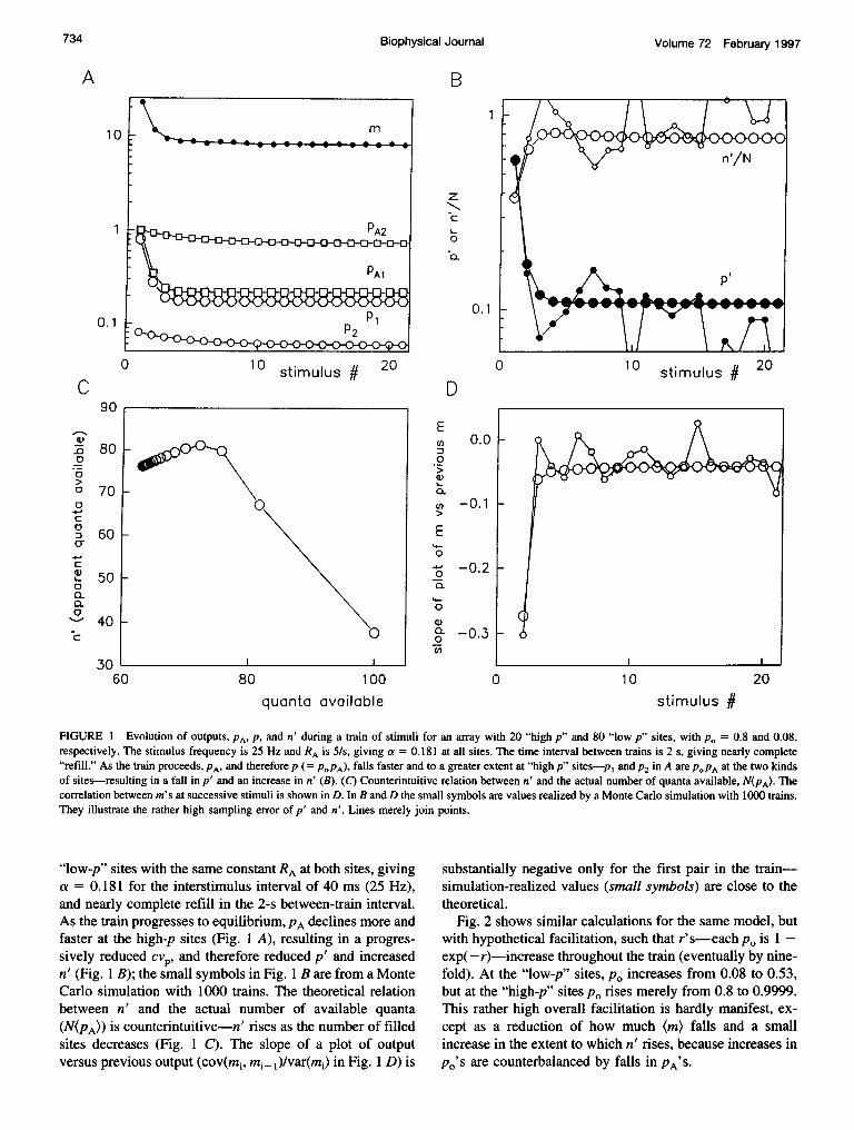
FIGURE 1 Evolution of outputs, PA, PI and n' during a train of stimuli for an array with 20 "high p" and 80 "low p" sites, with po = 0.8 and 0.08,respectively. The stimulus frequency is 25 Hz and RA is 5/s, giving a = 0.181 at all sites. The time interval between trains is 2 s, giving nearly complete"refill." As the train proceeds, PA, and therefore p (= POPA), falls faster and to a greater extent at "high p" sites-p1 and P2 in A are POPA at the two kindsof sites-resulting in a fall in p' and an increase in n' (B). (C) Counterintuitive relation between n' and the actual number of quanta available, N(PA). Thecorrelation between m's at successive stimuli is shown in D. In B and D the small symbols are values realized by a Monte Carlo simulation with 1000 trains.They illustrate the rather high sampling error of p' and n'. Lines merely join points.
"low-p" sites with the same constant RA at both sites, givinga = 0.181 for the interstimulus interval of 40 ms (25 Hz),and nearly complete refill in the 2-s between-train interval.As the train progresses to equilibrium, PA declines more andfaster at the high-p sites (Fig. 1 A), resulting in a progres-sively reduced cvp, and therefore reduced p' and increasedn' (Fig. 1 B); the small symbols in Fig. 1 B are from a MonteCarlo simulation with 1000 trains. The theoretical relationbetween n' and the actual number of available quanta(N(PA)) is counterintuitive-n' rises as the number of filledsites decreases (Fig. 1 C). The slope of a plot of outputversus previous output (cov(mi, mi+ )/var(mi) in Fig. 1 D) is
substantially negative only for the first pair in the train-simulation-realized values (small symbols) are close to thetheoretical.
Fig. 2 shows similar calculations for the same model, butwith hypothetical facilitation, such that r's- each p0 is 1 -exp(- r)-increase throughout the train (eventually by nine-fold). At the "low-p" sites, po increases from 0.08 to 0.53,but at the "high-p" sites po rises merely from 0.8 to 0.9999.This rather high overall facilitation is hardly manifest, ex-cept as a reduction of how much (m) falls and a smallincrease in the extent to which n' rises, because increases inpO's are counterbalanced by falls in PA'S.
10
1
0.1
0
90C
-o-0a)
C)
0
04-,c
0~Dc
0)L.0CLCLa
80 1
70 I
60 F
50 I
40 F
30 L6C 10 20
stimulus #
734 Volume 72 February 1997
1

Binomial Transmitter Release
A B
10 stimulus # 20
20 40 60 80quanta available
z
c
0
(a.
0.1
0
D
E:30
0
E
a0'4-00
a0
cn
0.0
-0.1
-0.2
-0.3
-0.4
100
10 stimulus # 20
10 20stimulus #
0
FIGURE 2 Same as Fig. 1, except for the addition of facilitation such that r (p0 = 1 - e-) grows with each stimulus, to a maximum of ninefold, at
both kinds of site. Overall mean m rises after an initial fall and is maintained higher than without facilitation (Fig. 1), and n'/N approaches unity (B) as
cvp becomes small. Note that the evolution of p' and mean m gives little hint of the rise in p0.
In Fig. 3 are shown plots from Monte Carlo simulations,of the second m (M2) versus the first (ml) with 200 or 5000stimulus pairs, here with one "high p" (p0 = 0.8) and 4 "lowp" (Po = 0.08) sites, either with po's unchanged at thesecond stimulus (Fig. 3 A) or with facilitation made so large(3.2-fold multiplication of r's at the second stimulus) thatM2 is larger than mlI (Fig. 3 B). Note: 1) the substantialnumber of occasions where output is higher than n' (for mlI,theoretical 1.885, 1.66 in A, 1.83 in B, for 200 trains); 2)depletion is not necessarily signaled by a decrease in m("paired pulse depression"), because it can be counterbal-anced by facilitation of po, but is always signaled by anegative correlation between M2 and ml; and 3) 200 stim-ulus pairs have been sufficient to show significant negative
correlation between M2 and ml. Similar simulations withhigh N (not illustrated) gave essentially linear relationsbetween M2 and ml and significant correlation (for 200iterations) whenever the absolute value of the theoreticalslope (cov(m2, ml)/var(ml)) was more than about 0.2, andalways if all sites start (nearly) full and p0's at some sites arehigh enough that outputs fall at the second stimulus. Thisagrees with the highly significant negative correlation be-tween second and first EPPs in trains reported by Elmqvistand Quastel (1965) in normal Ca2+/Mg2+ and curare, andthe lack of corTelation between EPP pairs in low Ca2+/highMg2+ (del Castillo and Katz, 1954b).A variation of the theme in Figs. 1 and 2 is given in Fig.
4, where the postulate is that stimuli have been given in the
10
0.1
0
C
100Q3)
00
0
0C)c
cr)aa-c
0
C)a/
80 F
60 F
40 I
- I
735Quastel
1

Volume 72 February 1997
A no facilitation
(NE
1.4
1.2
1.0
0.8
0.6
0.4
0.2
0.0
B high facilitation (x3.2)
0 1 2 3
2.22.01.81.61 .4
cN 1.2E
1.0
0.8
0.6
0.4
0.20.0
ml
(21)
(1
<ml>=1.19 n'=1.83
<m2>= 1.23
25)
(49)
, 11(5)
0 1 2 3
ml
FIGURE 3 Plots of m at a second stimulus (m2) versus m at a first stimulus (ml) for paired pulses; here the simplified array has one "high p" and four"low p" sites, with initial po of 0.8 and 0.08. Monte Carlo simulations were done with 200 pairs (large open circles, number of times value of ml realizedin brackets) or 5000 pairs (small filled circles, bars within points). In A, p0 are unchanged at the second stimulus, whereas in B, r are facilitated 3.2-fold,giving m2 somewhat bigger than ml. Note that 200 pairs are sufficient to show nonindependence of outputs, resulting from depletion and incomplete refillbetween the two stimuli.
presence of Sr2+ (Bain and Quastel, 1992a), producing aftereach stimulus a "tail" of release generated by residual Sr2+in the nerve terminal. The relative contributions of outputsfrom low- and high-p sites vary in time, because high-posites become more depleted and are less likely to have aquantum available to be released by the residual Sr2+ if, ashere, RA is the same for both types of site.
Not illustrated here is the correlation of outputs, at suc-cessive stimuli, with the sum of previous outputs. In thesimplest case (complete refill before the train, no refillbetween stimuli and uniform po's) successive outputs areE(mO) = NpoI, E(m2) = Npo2( - Pol)' E(m3) = NPo3( -
Po2)(1 - pol), etc. The variance of sums is given simply byN X E(m)(l- I E(m)), and the expected slope of mk versus(mI + M2 + ... + mk-1) is simply Pok, pO at the kthstimulus. However, with an array with varied po's and somerefill between stimuli, the most that can be said is that theabove slope roughly approximates (pok)(l + cvpok)Ikl forthe first few stimuli in the train-the correlations are asreadily detected as that between ml and m2-provided refillis nearly complete between trains.
Statistics of equilibrium outputs
With a continued train of stimuli, we can expect to reach anequilibrium in the sense that po's, a's, and expected valuesof ni no longer change, i.e., all ai's are a, all pi's are p., andE(ni+1) = E(ni) = E(n)-the assumption is that (average)
release is balanced by (average) replenishment. At thisequilibrium, for n equivalent sites,
E(n) = an + j3qXE(n) = an/(I -,3q0)
PA E(n)/n = a/(1 - 3q0) = a/(a + po- ap0)
E(n) = nPA
var(n) = nPA( - PA).
Writing p for POPA'
E(m) = np
var(m) = np(1- p)
cov(mi, min+l) =-np2,Bq0[=/3poq0(var(n)-E(n))]
cov(Mi, Mi+k) =-p2(f3qO)k.
(3a)
(3b)
(3c)
(3d)
(3e)
The formulae for PA, variance, and cov(mi, min+ ) are thesame as rigorously derived by Vere-Jones (1966). As pre-viously, one sets n = 1 for each site and sums over all Nsites to obtain the mean, variance, and covariance for thewhole array, obtaining the usual expressions for the com-pound binomial: (m) = N(p) and var(m) = N(p) (1 - (p)(1 + cvp2)), where eachp is POPA. Although the covariancescontain information on p0's, it may be noted that for a singlesite the negative of the ratio cov(mi, mi+1)/var(m) is fp.qJ(q. + p.(/a), which has a maximum of 0.125 at po = qo =a = 13 = 0.5, and at these values the covariance decreases
736 Biophysical Joumal

Binomial Transmitter Release
A
1000
1i00
10 -
0.1
0.01
0.00 1
a)D
Ec)
c-
o
D0-
.C00-
o 500 1000
1.0
0.8
0.6
0.4
0.2
0.00 500
0.5
co 0.40
*m 0.3
E0c> 0.20
.-&-
o 0.1L.
0.01000 0 500 1000
B1.0
a)D-0
cD
j
Q
0~
0-
0~
1000
0.8
0.6
0.4
0.2
0.00
time (ms)
500
time (ms)
U1)
0.
-C
0.-o
C)0L-
1000 0 500 1000
time (ms)
FIGURE 4 Theoretical outputs with stimulation in the presence of Sr2P, with one high-p site and five low-p sites and initial R. such that a half "resting"miniature frequency is from the high p site. At the high p site, higher output from the stimulus (80% of the stimulus available in A, 50% in B) producesmore depletion (second graph), causing the tail of raised miniature frequency for the high p site to be less than the combined tail from the low p sites. Inthe first two graphs filled points and heavy lines pertain to the high p site. After one stimulus (A) or a series of stimuli (B), the fraction of total output fromthe high p site (third graph, filled squares are fractions of (m)) is lowered. In B (four stimuli) it is assumed that [Sr2+] is less than in A, so that per-pulsem and depletions are less. The time constant for the removal of intracellular Sr2' is assumed to be 200 ms.
by 75% for each subsequent stimulus; at equilibrium,cov(mi, mi+k) is unlikely ever to be detectable for k 2.
"Automatic" changes in p' and n' withstimulation frequency
Theoretical equilibrium situations for a range of stimulusfrequencies are illustrated in Fig. 5. Here an array of 100sites has r's varying over a 1000-fold range. RA'S wererandomly assigned, with an exponential distribution with amean of 5/s. Three scenarios are shown: 1) r's (and po's)and RA' s remain constant; 2) r' s increase exponentially withstimulus frequency, 10-fold at 50 Hz and 100-fold at 100Hz, but RA's remain constant; and 3) r's increase as in 2),but RA'S grow in proportion to stimulus frequency, so that
a's are constant. Notably, unless RA' s rise with stimulusfrequency (3), potentiation of r's (2) is scarcely manifest innet outputs (Fig. 5 A), because high p0's become associatedwith depletion (Fig. 5 B). The apparent number of quantaavailable (n') always increases with stimulation frequency(Fig. 5 B), whether or not the true number of quanta avail-able (N(PA)) falls appreciably. Why this should be is shownin the cumulative distributions for the 100 sites ofp (PoPA)in Fig. 5, D-F. At 1 Hz the distributions are nearly the samefor all three scenarios (Fig. 5 D), and p's are very widelydistributed-a few can be near 1 because refill is nearlycomplete between stimuli, but at 50 or 100 Hz (Fig. 5, E andF), with or without potentiation of r's, the distributionsalways narrow (cvp diminishes and n' increases), eitherbecause refill is incomplete and high-p0 sites develop low
E000
L-o0
L-
c
E
1000
E000
o
UL)L-
E
100
10
1
0.1
0.01
0.00 1
0 500
737Quastel
I 174.

Biophysical Journal738
A
A
v00
1IE
B
0 50 100Hz
D
O0Sli0.001 0.01 0.1 1
p
100
10
0 50 100Hz
E100
80(n
(a 600
$ 40
C 20
Volume 72 February 1997
C
0
C
oj0~
0
0
o
C:
0 50 100Hz
F
0 -
0.001 0.01p
U1)5L)
U1)4-
0e)
-oE:3C-
0.1 1p
FIGURE 5 Theoretical equilibria at various stimulus frequencies for an array of N = 100 sites with widely varying r and RA (mean 5/s) for threescenarios: 1) constant r and RA (open circles); 2) r increases exponentially with frequency, loX at 50 Hz and lOOX at 100 Hz, but RA's are constant (filledcircles); and 3) same as 2), but RA's also rise with stimulus frequency so as to keep a's constant (open squares). The number of available quanta (N(PA))(large symbols in B) falls most in scenario 2), but this is accompanied by the greatest rise in n'; n' (small symbols in B) always rises with stimulus frequency,although p' (small symbols in C) may either rise (scenario 3) or fall (1 and 2). (D, E, and F) Cumulative distributions of P (= PJ)A) at 1 Hz, 50 Hz, and100 Hz, respectively. Distributions always narrow at high stimulation frequency, either because depletion is more at high-p0 sites and less at low-p0 sites(P,IA's become more uniform; scenario 1), or because no p can be more than 1.0 (potentiation raises initially low po's more than it raises initially highpD's; scenario 3), or for both reasons (scenario 2). In D-F the symbols are at every tenth point.
PA'S (1 and 2) and/or, even if refill accelerates with stimulusfrequency (3), because initially high po's, in contrast to lowpo's, have little room to grow, being limited to the maxi-mum of p = 1.Of course, the extent to which n' grows with stimulation
frequency depends upon the distribution and absolute mag-nitudes of po's and a's. The only scenario in which n' doesnot grow with stimulation frequency that I have been able tofind (not illustrated) is one where a's are related to po's insuch a way that low-po sites deplete as much as high-po sitesand po's either do not grow with stimulation frequency orare all so low that with facilitation none approaches unity.
Simulations for equilibrium: sampling error
Using Monte Carlo simulations with up to 160,000 stimuliin each sequence, and arrays of 40 sites with widely varyingpO's, it was verified that means, variances, and covariancesdid not differ significantly from values obtained by usingEq. 3 and summations. Depending on a's (RA's and stim-ulus frequencies), covariances between successive outputswere never more negative than -10% of the variances.Using small groups of k outputs (with subsequent averag-ing) to determine sampling error showed the ratio covari-ance/variance to be consistently biased upward by 1/k. Thestandard deviation of these ratios was close to k-0°5 (for k )
A0aV 0.1
0
Q
0.01
100
U)
U)4-0L5)-0D
c
80
60
40
20
1
1

739Binomial Transmitter Release
100, more for lower k), i.e., -0.05 for groups of 400outputs. Thus, one cannot envisage a statistically significantvalue for equilibrium covariance/variance with fewer thanfour groups of 400 stimuli.
Values of p' ( - var(m)/(m)) determined from valuesof (m) and var(m) within small groups and subsequentlyaveraged were unbiased, but small group estimates of n'((m)lp') were systematically biased upward, particularlywhen true p' was less than about 0.2; this bias became lessthan 5% for p' ) 0.3 and groups of 200 outputs or more.Notably, the sampling errors ofp' and n' at low p' are ratherlarge; the scatter shown in Figs. 1 B and 2 B (1000 samplesat each point) was typical.
Spontaneous loss of quanta from sites
For completeness, one must consider that filled sites mightat any moment become unfilled, by internal loss and/orspontaneous release, both loss and refill being continuousprocesses. An exact mathematical result can be obtained bydividing the time interval between stimuli (7) into a suc-cession of small Bt's and taking limits. Assume rate con-stants for internal loss, RL, spontaneous release, R., andreplenishment, RA. In each St loss is (RL + R.)n5t, and refillis RA(n - n)St, where n is the number of filled sites at anymoment. At the limit one obtains the differential equationdn/dt = RAn -(RA + RL + R0)n. This is a standard poolmodel with entry and exit; n changes exponentially with rateconstant T = 1/(RA + RL + RO), asymptoting to n' =
nRA/(RA + RL + R.). Previously a was 1 - exp(- TRA); itnow becomes 1 - exp(- T/T), and 1B becomes exp(-TIT),which is less than previously. Equations 2 and 3 are mod-ified only by the new definition of a and 13 and by replacingn by n' in equations for E(ni) or E(ni+ I) in which n appears.The net effect of loss is twofold: 1) maximum PA = RAT,which is < 1, and 2) reduction of covariances.
Relation between po and stimulus-evoked release rate(s)
It has already been pointed out that po's must be constrainedto less than unity in modeling how an array of synaptic sitesmay behave if po's are to be modulated, e.g., hypothesizingthat po is increased by raising external [Ca2+], or withfacilitation. The problem of how to do this disappears if oneconsiders po to result from a succession of small probabil-ities within a total release time t. To be precise, let ussuppose that these probabilities are r1&t, r25t, * - *, rj&t, ....etc. in succession after a stimulus. Here rl, r2, etc. arerelease rates, which can have any positive value, provided Stis made sufficiently small. Assume further that t is so briefthat the refill possibility is negligible, i.e., no more than onequantum may be released. Then the chance of a quantum
chance of a quantum from a filled site not being released ineach time period i is Qi = exp(-r,6t); the chance of it not
being released in the whole period t is the product of allQi's. Hence,
pO = 1 - exp(-&t(ri + r2 + r3* )) = 1-exp(-r0t),where r. is the average ri over time t. These r0t' s correspondto the r' s already used in modeling how outputs may changewith "global" facilitation (Figs. 2, 3, and 5).
Release asynchrony
There have now been many experimental observations ofthe time course of release; although the major portion oc-curs in a time window of less than a millisecond (e.g. Katzand Miledi, 1965; Bain and Quastel, 1992a), the situation iscomplicated by a tail of raised frequency of "miniature"quantal events that decays with a time constant on the orderof 100 ms (e.g., Hubbard, 1963; Bain and Quastel, 1992b),at least some of which may or may not-the decision isarbitrary-be included in the evoked synaptic signal.No information currently exists on the extent to which
observed dispersion may represent variation between ratherthan at sites. Nevertheless if within-site time dispersion ofhigh release probability exists at all, stochastic replenish-ment implies that a single site sometimes releases more thanone quantum after a stimulus, because there is some chance
TABLE 2 Increases in apparent quanta/site (n.) at a singlesite with one quantum, and decreases of apparent p (Pa)produced by taking into account partial replenishment duringrelease period
T/I = 0.5 TIT = 1.0Apa/Anla = -0.95 + 0.20p0 Apa/Afna = -0.96 + 0.32p0
PO p An* P An*
0.125 0.105 0.8 0.117 0.80.25 0.180 1.1 0.218 0.90.5 0.282 1.6 0.387 1.20.75 0.348 2.6 0.522 1.70.875 0.373 3.6 0.580 2.30.95 0.385 4.7 0.612 2.90.99 0.392 6.5 0.628 4.0
TIT= 2.0 TIT= 4.0APa/Afna = 0.98 + 0.45p0 APa/Afna = 0-99 + O.55p0
pO p An* p An*
0.125 0.123 0.7 0.125 0.70.25 0.241 0.8 0.249 0.80.5 0.464 1.0 0.495 0.90.75 0.671 1.3 0.740 1.20.875 0.770 1.7 0.861 1.50.95 0.827 2.2 0.933 1.90.99 0.857 2.9 0.972 2.5
Listed An* is the percent change in apparent n (from unity) for tfflT =0.01; for other teftlT Alna is proportional to tef0T. In each case the firstcolumn on the left gives p0, and listed p is POPA Effective refill betweenstimuli is always 1 - exp(-TIT). Changes in apparent p (An-P) are propor-
being released (if available) is 1 - prob(no release). The tional to Anaand dependent upon p. according to the formula.
Quastel

Biophysical Journal
of refill while release probability is still high. The effects ofthis on means and variances were calculated using thegeneral scheme above, with a succession of small po's insmall W's. The results are shown in Table 2, which isexplained further in the Appendix. The general result is thateach site indeed behaves on average as though it had morethan one quantum available for release (apparent n, na > 1),but apparent p (Pa) is decreased; mean output is increasedless than variance. By and large, effects are small if mostrelease occurs within a time that is on the order of 1% orless of the replenishment time constant. In the rest of thissection it will be assumed that instantaneous release is avalid approximation for release by stimuli.
Modification of statistical measures by quantalamplitude and stochastic channel closing
Rarely can released quanta be counted directly in an exper-iment. Instead one measures signals that represent responsesto individual or summed quanta. Assuming linear summa-tion, if quanta all give rise to a response of constant ampli-tude (or area, if time integrals are measured) h, the meanresponse is scaled by h, the variance and covariances by h2,and the third moment by h3. Otherwise, the scaling dependson whether nonuniformity in h occurs at every release site,or whether h varies between release sites, or both; modelscurrently employed in the analysis of CNS synaptic signalsdiffer in this respect (Redman, 1990; Walmsley, 1993; Jacket al., 1994).
(a) Quantal responses are constant at each release site butvary between sites
In this case, mean, variance, covariances, and third momentare scaled at each site by its h, h2, h2, and h3, and the mean,variance, etc. for the array are obtained by addition, i.e., theonly general formulae are E(S) = - (hp), var(S) =- (h2(p - p2)), etc., where S denotes either signal height orarea. Notably, var(S) is less than if h varies at each releasesite. For example, suppose there are three release sites withh = 1, h = 2, and h = 3, respectively. Then a "success" atevery site (three quanta) always has S = 6, but if quantamay have h = 1, 2, or 3 at each site, S can vary between 3and 9.
(b) Quantal responses vary at every release site (andnot between)
In this case moments can be calculated directly. The mo-ments about 0 at each release site, ,u,l', and p', are eachp times the respective moments of h about 0, i.e., p(h),p((h)2 + var(h)), and p((h)3 + 3(h)var(h) + H3), respec-tively, where H3 is the third moment of h about its mean.
Therefore, for each release site,
E(S) = (S) = p4 = (h)P
var(S) = ,U2- (t)2 = (h)2p(1 + cv' - p)
S3 = F3 - 3(p4)(p4) + 2(,4)3(4)
= (h)3p[(1- p)(l - 2p) + 3p(l -p)CV2 + h3')].
Here S3 is the third moment of the signal; CVh is thecoefficient of variation of h and h3' is H31(h)3.Summing over N release sites gives
E(S) = (S) = N(p)(h) = (m)(h)
var(S) = (S)(h)(l- p' + cv2) (5)
= (h)2(var(m) + (m)cv2)and
S3 = (h)3[M3 + (m)(h3' + (1 -p)CV2)],where p' is, as before, (p) (1 + cvp) and (m) has beenequated with E(m). The first expression for var(S) gives p'and hence var(m) if CVh as well as (h) can be inferred from"miniatures."The covariance between successive responses to stimuli
is, of course, simply scaled by (h)2, assuming that there is nocovariance of quantal amplitude from one stimulus to thenext.
It is notable that the coefficient of variation of the signal,cvs, is given by
cv2 var(S)/(S)2 = (1- p' + cv2)/(m).For a Poisson distribution, with p' = 0, (m) is given by(S)2/var(S) if cv2 = 0. Because p' is usually less than 0.5,and cvh is unlikely to be more than 1, (S)2/var(S) generallygives an approximation of (m) that is accurate within afactor of 2 or so.
(c) Quantal responses vary both between sites and at sites
In this case one sums as in (a), taking into account thevariance, etc., of h at each site using Eq. 4:
E(S) = E ((h)p); var(S) = E ((h)2p(1 + cv' - p))
S3 = , ((h)3p[(1 - p)(l - 2p) + 3p(l - p)cv2
Contribution to the variance of stochastic channel closing:estimation of channel amplitude
If signals are voltage signals with the decay rate dominatedby the cell input impedance, the coefficient of variation ofsignal areas (time integrals) is the same as that of signalheights, but if currents are measured it is greater, because ofthe contribution to variance of stochastic closing of thechannels underlying the quantal responses. For exponen-tially distributed channel durations I calculate (see Appen-
740 Volume 72 February 1997

Binomial Transmitter Release
dix 3) that cv2 for the signal area is higher than for height byjust 1I(n,) whatever the signal-to-signal distribution of nc,the number of open channels in each. An important assump-tion here is that all quantal responses and all channel open-ings occur close enough in time that net signal heightrepresents all channels that open. If not, one could obtain(nc) and hence channel amplitude, h,, from means andvariances of signal heights and subsequent areas somewherein the decay phase, beyond which there is no new channelopening. Of course, to estimate hc in this way, artificiallyaligned miniatures would serve as well as responses tostimuli, and in either case the noise component of varianceswould have to be subtracted.
The area product
In practice the determination of means and variances (andcovariances) from experimental data is not simple. It gen-erally involves finding a baseline for each signal and adecision whether to measure maximum height, the height atthe average maximum (the latter is unbiased by noise butmore biased by time dispersion of release), or signal area,which is relatively sensitive to any error in baseline.A way to avoid such problems and to extract some added
information from the data is to make use of the covariancesof point values with signal sums. For want of a better term,I call these the "area product" (A). This function can bedetermined by accumulating from the record for each stim-ulus (YI, Y2, y3, .-. . etc.), including prestimulus values, theproduct of each point value yj with the sum of all values inthe record (S), while also obtaining mean yj's and mean S.Designating as Aj the covariance at point j, it turns out thatthe sum of Al's for all points in the record is exactly thesame as the variance of S, as calculated simply from valuesof S for every record (see Appendix, 4 i):
E Aj = var(S) (6a)
where the summations (for S and E A) are over all j, towhere the signals have decayed to a small fraction ofmaximum. Moreover, if certain conditions are met,
Aj = E(yj) var(S)/E(S). (6b)
To derive Eq. 6b, consider the signals obtained from asingle release site that releases quanta with a time sequenceof probabilities giving rise to a release time course p(t) withtotal probability p (= I p(t)'s). Each quantal response has atime course h(t), the mean signal being the convolution ofh(t) and p(t). For simplicity let us choose a time base so thatthe time integral of the response, E h(t), is equal to unity.We have uncorrelated records. In any single record there iseither no quantum or one; signal area (S) is 0 or 1. There-fore, for each record the cross-products of point values withS are the same as the original record (Fig. 6 A). For all of therecords, at pointj, this product has the expected value E(Syj) =
ance of the point value with the sum of the signal (S), i.e.,((yj - (y*))(S - (S))), is
Area product for 1 site at pointj = Aj= cov(yj, S) = E(Sy) - E(S)E(y) = E(y) - pE(y)
= (1 -p)E(y)
Because with quantal area = 1, var(S)/E(S) = (1 - p), thisresult corresponds to Eq. 6b.
If the quantal response has area h, S is either h or 0,E(Syj) = hE(yj) and E(S) is hp; cov(yj, S) = h(l -p)E(yj),and Eq. 6b is again correct. In Fig. 6 A the terminology isslightly different; here the quantal responses decay expo-nentially and have height h and area hTr, to contrast the resultwith what occurs with single channels, with exponentiallydistributed lifetimes (Fig. 6 B), having the same height andmean area as the quanta in Fig. 6 A.Now it is important to note that the area product at each
point is a covariance and therefore is additive for indepen-dent stochastic processes, and that because Eq. 6a is anumerical identity, scaling of the area product by quantalheight and variance is just the same as that of variance ofsignal sums.Summing over N sites with different p's, one finds that
there are two essential provisos for the area product functionA(t) to recapitulate the time course of (y(t)) (Eq. 6b), namely1) every quantal response has the same time course, h(t)lh,and 2) quanta of different amplitudes have the same p(t)lp.Thus the time partitioning of var(S) provided by A(t) canindicate whether these provisos are not met:
1. Release sites producing quanta of different amplitudeshave differing p(t)lp. Example: Release at large quanta sitesis delayed until the signal from small quanta has decayed-early values of Aj/(yj) pertain to small quanta and late valuesto large quanta.
2. If stimulation causes the appearance of quantal re-sponses differing in h(t)lh, the more prolonged contributemore to late values of Aj and the ratio Aj/(yj) is eventuallythat expected for the most prolonged alone. Example: Oneset of quantal responses is "filtered" by electrotonic con-duction and therefore is prolonged, whereas others are not(see e.g., Jack et al., 1994).
3. If there is postsynaptic nonlinear summation of guantalresponses, the height of quanta is in effect reduced as quantaare superimposed: Aj/(yj) characteristically dips when (yj) ishigh.
4. Always, with voltage clamp, because quantal re-sponses, each a composite of currents through a number ofchannels with stochastically varying lifetimes, never haveabsolutely identical time courses.The last breach is of particular interest as a common com-
plication, and because it leads to a simple method of determin-ing unit channel amplitude, provided other complications canbe ruled out, the number of channels per quantal response is
E(yN). The expected value of mean area, E(S), is p. The covari-
741Quastel
fairly low, and recording noise is not overwhelming.

Volume 72 February 1997
A uniform quanta
y(t)
--t)
B channels
Sy(t)
<Sy(t)>
y(t) Sy(t)
-iF-I- --
(y(t) > <Sy(t)>
A(t)
A(t)/<y(t)>=h(l-p)T +htt
FIGURE 6 The theoretical basis for the area product. In A a single site on stimulation may or may not release, with a time-distributed probability p, aquantum producing an exponentially decaying response with unit area. Four samples of individual responses are shown above and to the left, and thecorresponding cross-products with area, which are the same. Theoretical averages for a large number of such records are shown below, with thecorresponding A(t) and the ratio A(t)/(y(t)). The latter is (1 - p) multiplied by the quantal area, height (h) multiplied by time constant (T). In B the unitresponse is the opening of a single channel of height h, with exponentially distributed lifetimes with mean T. Brief channels give a brief small Sy(t), whereasprolonged channels give prolonged large Sy(t); the ratio of the area product (A(t)) to (y(t)) rises linearly with slope h (see Appendix, 4 ii). In the plots shownthe scales of A(t) and A(t)/(y(t)) have been chosen for convenience.
In Fig. 6 B, a patch with a single channel is envisaged;each channel has an Sy(t) that is a square pulse with heightproportional to its duration; durations are exponentiallydistributed. For channels with mean duration Tc and ampli-tude hc, opening at the same time with probability p, sum-ming all products of probability and outcome (see Appen-dix, 4 ii) gives
A(t) = (y(t))(hcT(1 - p) + hct), (6c)
where (y(t)) is, of course, hcp exp(-t/Tc).As it turns out, the linear growth of A(t)/(y(t)) versus t
with slope hc remains if quantal responses reflect groups ofchannels opening; the expected value when the signal be-gins is the same as if quantal responses were uniform intime course (see Appendix 4 ii). Moreover, taking as unittime the sampling interval (i.e., simply adding point valuesto make sums), Aj/(yj) grows linearly with j, with slope hc.
If channels do not all open simultaneously, the theoreticalvalue of A(t) is more complicated. However, calculations(and simulations; Fig. 7) show that the linear growth ofAj/(yj) with slope hc remains, at least after the peak of thesignal, provided most openings occur before most closings.If channels flicker between open and closed states (theseclosings do not count in the previous sense), but net opentimes remain exponentially distributed, then the hc oneobtains is the true hc multiplied by the fraction of time that
the channels are open. This is equally true for hc found fromthe coefficients of variation of signal height and area (seeabove), which rests on the same assumptions about channelbehavior. Moreover, in both cases, the "extra" variancedisappears with sufficient electrotonic filtering. To obtain hcin practice, supposing that all but one kind of channel havebeen eliminated pharmacologically, and responses are froma set of synapses with much the same p(t)/p, one wouldobtain parameters for the least-squares best fit to baselinenormalized Aj/(yj) = a + bj, for j past the peak of (yj),including only j's with well-defined (yj) > 0, and weightingby (yj)3 (see Appendix, 5), with b being the putative valueof hc. As with the other method for determining hc, this isequally applicable to artificially aligned spontaneous min-iatures, or, indeed, evoked signals grouped according topeak amplitude.
Noise
As a stochastic process not time-locked to the stimulus,recording noise contributes a positive value to A(t) that isthe same at all times, including prestimulus; for any simplelow-pass filter, the expected value turns out to be the noisevariance of the unfiltered records. Noise also adds some-what to the noisiness of the area product; but this effect issmall if responses can be seen at all. In the simulation in
A(t)
A(t)/<y(t)>=h(l1 -p)-r~
742 Biophysical Journal
Binomial Transmitter Release
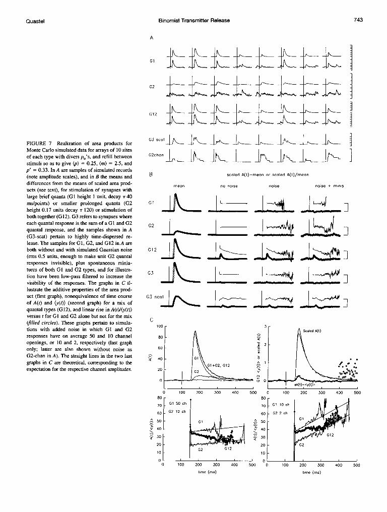
FIGURE 7 Realization of area products forMonte Carlo simulated data for arrays of 10 sitesof each type with divers p0's, and refill betweenstimuli so as to give (p) = 0.25, (m) = 2.5, andp' = 0.33. In A are samples of simulated records(note amplitude scales), and in B the means anddifferences from the means of scaled area prod-ucts (see text), for stimulation of synapses withlarge brief quanta (GI height 1 unit, decay T 40ms/points) or smaller prolonged quanta (G2height 0.17 units decay T 120) or stimulation ofboth together (G12). G3 refers to synapses whereeach quantal response is the sum of a G 1 and G2quantal response, and the samples shown in A(G3-scat) pertain to highly time-dispersed re-lease. The samples for GI, G2, and G12 in A areboth without and with simulated Gaussian noise(rms 0.5 units, enough to make unit G2 quantalresponses invisible), plus spontaneous minia-tures of both GI and G2 types, and for illustra-tion have been low-pass filtered to increase thevisibility of the responses. The graphs in C il-lustrate the additive properties of the area prod-uct (first graph), nonequivalence of time courseof A(t) and (y(t)) (second graph) for a mix ofquantal types (G12), and linear rise in A(t)/(y(t))versus t for G1 and G2 alone but not for the mix(filled circles). These graphs pertain to simula-tions with added noise in which G1 and G2responses have on average 50 and 10 channelopenings, or 10 and 2, respectively (last graphonly; latter are also shown without noise asG2-chan in A). The straight lines in the two lastgraphs in C are theoretical, corresponding to theexpectation for the respective channel amplitudes.
A
G2 X, N- -X\,--Xi,4,i-- -J
G12 K -\ -N \-
G3 scat\
<
G2chan-
<-
]- P
F
I
IB
mean
Gl |2
scaled A(t)-mean or scaled A(t)/mean
no noise
LL
noise noise + minis
J.J-]-"
0l2 II J 2i
G0 12 I- J J ]
03 L- JIJ]G3 sct
C100
80
60
40
20
0
3
o0
0 100 200 300 400 50080 -
70 -
60
A- 50 -
v 40
30 -
20 -
10 -
0 -
Gl 50 ch
G2 10 ch
A
v1-
cC
0 100 200 300 400
time (ms)501
80
70
60
50
40
30
20
10
00)O
A 1-5coled A(t)
I *
sA(t)-<cy(t)>
0 100 200 300 400 500
lGl 10 ch
-2 2 ch0 1
012
0 100 200 300 400 500
time (ms)
Gl
G12
l-
743Quastel
lll.... I

Biophysical Journal
Fig. 7 (see below), so much noise was added that the smallquantal responses cannot be seen, but 200 records with 500quanta in all yield a very "clean" A(t).
Spontaneous miniatures may constitute an importantsource of "noise." This, too, can be eliminated by subtract-ing from all values of A(t) the average prestimulus value.However, if the total area of miniatures in records is muchmore than the total area of signals, the resulting point-to-point noisiness of A(t) may limit the usefulness of the areaproduct to determination of noise-unbiased var(S) by sum-ming Aj's after baseline correction.
Monte Carlo simulations
Fig. 7 illustrates how well area products conform to expec-tation and extract otherwise inaccessible information fromsimulated data (samples in Fig. 7 A). From series of 200synaptic signals with (m) = 2.5, and uniform quanta, areaproducts had virtually the same time course as averages(Fig. 7 B), either with relatively large brief quantal re-sponses (GI) or small prolonged quanta (G2), or quantaeach consisting of the sum of a G1 type and G2 typequantum (G3). To facilitate visual comparison in Fig. 7 B,the area products, after subtracting prestimulus values, werescaled to have the same area as the means; the differences ofscaled area product, sA(t), from means ((y(t))) are plotted tothe right of the means in Fig. 7 B for three scenarios: norecording noise, Gaussian noise sufficient to obscure quantaof the G2 type, and the same noise plus random miniaturesof both GI and G2 types at an average of one each perrecord. In contrast, for synaptic signals corresponding toGI- and G2-type synapses being stimulated simultaneously(G12), the differences are substantial. Correspondingly,plots of ratios of A(t)/(y(t)) versus time (thin lines) are flat(but noisy when (y(t)) is low), except for the G12 situation,where this ratio declines as smaller, more prolonged G2quanta become the predominant components of both A(t)and (y(t)). In the G3 scat simulation, highly time-dispersedG3 quantal release (see samples in Fig. 7 A), the differenceof sA(t) from (y(t)) wobbles, probably because about 500quanta was insufficient for the actual release dispersion toclosely approximate p(t)lp late in the signals.
For Fig. 7 C the simulation was continued to 1000records, for a situation in which Gl quanta contained onaverage 50 channels and those of the G2 type 10 channels,so that hc (but not Tc) was the same for both types. Simu-lated recording noise was included in these records, but notminis. The first graph illustrates the additive properties ofA(t) for the mix (G12); A(t) is indistinguishable from thesum of A(t)'s for GI and G2 alone, the difference (line nearzero) being negligible at all times. The second graph shows(y(t)) for the mix, and its scaled A(t); the differences (smallcircles) are essentially identical to those expected (nearbyline) for an A(t) equal to the sum of A(t)'s for GI and G2alone. The filled circles on the right show SDs of sA(t) andy(t), respectively (each X 100), illustrating that the intrinsic
noisiness of the area product is not much more than thenoisiness of the mean.The third graph in Fig. 7 C shows how for GI or G2 alone
the ratio A(t)/(y(t)), past the peak of the signal, indeed growslinearly with a slope of hc per point, whereas for the mix(G12) the ratio gradually falls from an appropriate value forGI alone (at the start where G2 responses are negligible) tothe value for G2 alone. This is also seen in the last graph,where the model was modified by ascribing an average of10 channels to GI quanta and an average of 2 channels toG2 quanta (also see the bottom sample in Fig. 7 A). Thenoisiness of the plotted ratios (and initial high values)comes from including points with very low (y(t)O's thatwould not be included in finding hc by least-squares fitting.
However, in the last graph in Fig. 7 C, an intrinsicambiguity of the area product is exemplified in that with theoutput mix (G12 filled circles), the plot of A(t)/(y(t)) versustime could here be mistaken for that produced by a singleset of quanta, i.e., flat until too noisy for the late rise to beascribed to anything but noise. Using subgroups of signalsselected by amplitude would resolve this ambiguity.
Dealing with drift and finding sequential signal covariance
Another problem in analysis is how to compensate for anydrift (nonstationarity) in the signal, i.e., m's and/or h'strending up or down. This can add substantially to variances(and reverse covariances); being able to compensate adds tothe variety of usable stimulation paradigms (e.g., Elmqvistand Quastel, 1965). Assuming stimulation at a constantfrequency, one way to exclude effects of such drift is bydetermining variance (and covariance) within small groupsof sequential records. The smallest possible group is 2;determination of the area product now reduces to taking foreach record the point-to-point difference of this record(yij's) from another nearby (Yi+k,'S) to obtain a new seriesof numbers (zj's) and accumulating products (zj X z). Cor-responding to Eq. 6, the expected mean of these turns out tobe
E(zj I z)/2 = AI = E(yj)(var(S) - cov(Si, Sj+j)/E(S) (7a)
E Aj' = var(S) - cov(Si, Si+k). (7b)
Because cov(Si, Si+k) is negligible for k . 2, using differ-ences between records both one apart and two or morestimuli apart gives both var(S) and cov(Si, Si+,). Withsimulations, values of equilibrium variance determined inthis way were found to be unbiased, but had a samplingerror increased by about 50%; using two such differencesfor every output reduced to no more than 10% the increasein sampling error. Obtaining covariances by also usingdifferences between sequential outputs gave sampling errorsfor covariance/variance 25% higher than when determinedin the usual way, and no bias.An alternative that essentially eliminates even rapid drift
effects is to take the sum of point-to-point differences from
744 Volume 72 February 1997
Binomial Transmitter Release
values k stimuli before and k stimuli after, i.e., zj = 2yij-Yi+kj - Yi-kd * Then,
Ej E(zj I z) = 6 var(S) - 8 cov(Si, Si+k) + 2 cov(Si, Si+2k)
Point-to-point variance and the third moment of S
The area product should not be confused with the point-to-point variance of signals, which is quite different. At asingle site, with one quantum to release, one has generally
var(y(t)) = p(t) * [(h(t))2(1 + CVh(t))] - (p(t) * (h(t)))2
where * denotes convolution. In the case of a Poissondistribution of outputs, which provides an excellent approx-imation when p' << 1, and multiple sites, this equationreduces to
var(y(t)) = m(t) * [(h(t))2(1 + CV2(t))]
where m(t) is the time course of quanta appearing. If quantalresponses consist of currents through not too many chan-nels, cv2(t) can become substantially different from cv2(0)because of the "extra" variance introduced by stochasticchannel closing. For channels of uniform amplitude, open-ing simultaneously and closing randomly, one has for point-to-point variance of quantal responses,
var(h(t))/(h(t)) = hc + (h(t))(Cv2(o) - hc/h(O))
which, of course, provides yet another method for obtaininghc from artificially aligned miniatures. The terms with hcdisappear if signals are overfiltered (e.g., electrotonically, orif one is recording voltage) with a time constant >Tc.
For a Poisson distribution, the third moment of y(t) isgiven by m(t) * [(h(t))3(l + x)], where x is the sum of termsthat disappear if quanta are uniform in height and timecourse.
For the third moment of S (S3), the analog of Eqs. 6a and6b is obtained by taking the mean product B. = ((yj -
(yj))(S -()2 . The sum of Bj's is numerically identical toS3, and B(t) has the same time course as (y(t)), subject to thesame provisos as for A(t). For quanta that vary in timecourse because of stochastic closing of channels, Bj/(yj) -
2Aj/(yj) grows linearly with j2, with slope hc.
"Spontaneous" release
In the original quantal analysis of synaptic signals, at theneuromuscular junction, it was shown that the quantal com-ponents of the stimulation-evoked synaptic signal corre-spond (in amplitude, time course, and sensitivity to postsyn-aptically acting drugs) to the "miniature" signals thatrepresent spontaneous release of quanta of neurotransmitter(del Castillo and Katz, 1954a, 1956). There are now manyreported examples of miniatures at diverse synapses.The frequency of "spontaneous" miniature signals can be
increased in a variety of ways, but from the statistical pointof view it does not matter whether release is truly sponta-
neous or is evoked by a steady stimulus such as nerveterminal depolarization or raised osmotic pressure. In eithercase, miniatures occur apparently randomly. Vere-Jones(1966) has shown that if there are a limited number N ofrelease sites and at each site quantal discharge is followedby a waiting time (presumably stochastic and exponentiallydistributed) before release can again occur, outputs will beunderdistributed relative to a Poisson. This is manifested inthree ways: 1) the variance is less than the mean for num-bers of miniatures in nonoverlapping time periods; 2) thereis a small negative covariance between such numbers; and3) the rate of occurrence of miniatures is transiently dimin-ished after each miniature.
Variance, means, and covariances of outputs innonoverlapping time periods
These are derived from Eq. 3 by envisaging a succession ofsmall p0's (and a's) in small &t's, adding outputs for a giventime period T, and obtaining variance and covariances ofthese outputs by adding variances and appropriate (nega-tive) covariances. By taking limits, I obtain the followingfor outputs (o) from a single release site with rate of releasefrom a filled site, RO, rate of refilling of an empty site, RA,and rate of internal loss from a filled site, RL. The netrelease rate, R, is equal to RORAT, where , the time constant,is I/(Ro + RL + RA) and RAT is the expected number offilled sites at any moment (see also above):
mean = E(o) = RT
var(o) = RT{1- 2Ri{1 - (1 -e-W)/W]}
cov(oj, oi+l) = -[R1-e-W)]2 (8)
cov(oj, o°+k) = cov(oj, oi+i)e(k )W
where W denotes T/T. The formula for variance differs fromVere-Jones (1966), which has a misprint.
Ignoring the hypothetical RL, the ratio of variance tomean is close to unity if R. << RA or R. >> RA, or if T <<ir, otherwise the ratio progressively declines as T is in-creased, to 1 - 2RT, which has a minimum of 0.5 at R =
RA. The covariance between successive outputs, cov(oi, oi+ ),has a (negative) maximum relative to variance when T issomewhat greater than r, the ratio of covariance/variance ismost negative when RO = RA, at which it is only -0.133.
For N sites with different RO, etc., one adds means,variances, and covariances to obtain the behavior of thearray. I find that if R. varies widely and RA is similar at theN sites or varies randomly between sites, minimum vari-ance/mean is about 0.6 and is found at T about 10/(RA) andwith (R)T on the order of one per site. If at some sites R. ismore than RA, a T can usually be found at which covariance/variance is about -0.1 (i.e., is potentially detectable exper-imentally with long data runs), in a situation in which
745Quastel
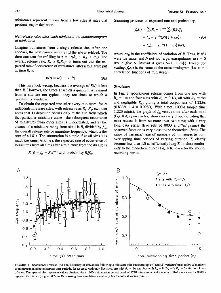
Volume 72 February 1997
miniatures represent release from a few sites at rates thatproduce major depletion.
Net release rates after each miniature: the autocorrelogramof miniatures
Imagine miniatures from a single release site. After oneappears, the next cannot occur until the site is refilled. Thetime constant for refilling is ST = l/(R? + RA + RL). Theoverall release rate, R, is RORAT. It turns out that the ex-pected rate of occurrence of miniatures, after a miniature putat time 0, is
R(t) = R(1 - e-tT). (9a)This may look wrong, because the average of R(t) is less
than R. However, the times at which a quantum is releasedfrom a site are not typical-they are times at which aquantum is available.To obtain the expected rate after every miniature, for N
independent release sites, with release rates R,, R2, etc., onenotes that 1) depletion occurs only at the site from whichthat particular miniature came-the subsequent occurrenceof miniatures from other sites is uncorrelated, and 2) thechance of a miniature being from site i is Rj divided byfin,the overall release rate or miniature frequency, which is thesum of all R's. The summation is simple if at all sites T ismuch the same. At time t, the expected rate of occurrence ofminiatures from all sites after a miniature from the ith site is
Ri(t) =. - Rie-tlT with probability Ri/fm.
Summing products of expected rate and probability,
fm(t) = > R e-tT I (Ri)2/f
=m- e-"T(R)(1 + cv2) (9b)
= fm - e'T(1 + cv')/N),where CVR is the coefficient of variation of R. Thus, if R'swere the same, and N not too large, extrapolation to t = 0would give N; instead it gives N/(1 + cv2). Except forscaling, fm(t) is the same as the autocorrelogram (i.e. auto-correlation function) of miniatures.
Simulation
In Fig. 8 spontaneous release comes from one site withRo = 1/s and four sites with Ro = 0.1/s, all with RA = 5/sand negligible RL, giving a total output rate of 1.225/s(0.833/s + 4 X 0.098/s). With a total 1000-s sample time(1220 minis), the graph of fm versus time after each mini(Fig. 8 A, open circles) shows an early drop, indicating thatmost release is from no more than two sites; with a verylong data series (five sets of 8000 s; filled points) theobserved function is very close to the theoretical (line). Theratios of variance/mean of numbers of miniatures in non-overlapping time periods of varying duration, T, clearlybecome less than 1.0 at sufficiently long T, in close confor-mity to the theoretical curve (Fig. 8 B), even for the shorterrecording period.
B
0
(n
T E
0
C:aU)Ea)
a
RA=5/S1.0
0.9
0.8
0.7
0.0 0.2 0.4 0.6 0.8 1.0
time (s) after mini
0.1 1 10
non-overlapping time period (s)
FIGURE 8 Spontaneous release. (A) The frequency of miniatures following a miniature (the autocorrelogram) and (B) variance/mean ratios of numbersof miniatures in nonoverlapping time periods, for an array with only five sites, one with Ro = 1/s and four with Ro = 0.1/s, with RA = 5/s for both kindsof sites. The open circles represent values obtained for a 1000-s simulation period (total of 1220 miniatures), and the small filled circles are for 8000 srepeated five times (to give SE's in B), showing how simulation eventually fits theoretical values (lines).
A1.8
1.6
1 .4
0
CTU)
.-U)
1.2
1.0
0.8
0.6
0.2 --I
746 Biophysical Joumal
r-
0.4

Binomial Transmitter Release
DISCUSSION
For any series of fluctuating synaptic signals there is a meanand variance, and if the mean and variance of the quantalcomponents are known, one can obtain the mean, (m), andvariance, var(m), of numbers of quanta released, and, fromthese, p' = 1 - var(m)/(m) and n' = (m)lp'. What is themeaning of n' and p', except as parameters that sometimes(Table 1) give a good approximation of the output distribu-tion? In terms of the simple binomial model, in which all Nindependent release sites are equivalent (have the sameprobability of release p), n' is N, which must be invariantunder all experimental conditions and no less than themaximum output obtainable under any conditions. Henceexperimental results showing n' to vary with stimulationfrequency and/or ambient Ca21/Mg2+, at both vertebrateand invertebrate neuromuscular junctions (for referencessee McLachlan, 1978), negate this model. The question nowarises whether n' might instead represent the number ofactive sites, rather than the total number. Here two distinctuntenable models seem to be confounded in the literature. Inthe first, an active site is one with a quantum available; n'is their number and p' is the (uniform) output probability ofthese, here designated po. For this to apply, the number ofavailable quanta would have to be constant from stimulus tostimulus, despite fluctuations in release-i.e., the modelpresupposes a presynaptic monitor that counts outputs andthen adjusts the available quanta at every site accordingly.Apart from its implausibility, this model denies the princi-ple of release site independence, invalidating the use ofbinomial statistics. The second model is a constrained spe-cial case of the compound binomial in which n' active sitesall have the same p' = P = POPA' PA being the probabilityat any moment that an active site has a quantum available,the other N-n' sites being silent (p = 0). This model isself-contradictory, because release sites are presumed to beboth identical and dissimilar simultaneously; if sites areactive and can ever release a quantum, they do so with thesame probability, but at the same time each site differs fromothers with respect to an absolute threshold for an extracel-lular Ca2+/Mg2+, or for stimulus frequency, depending onwhich happens to have been varied experimentally, belowwhich it is silent. Thus the mathematical simplicity of thesimple binomial model is incompatible with any simplemodel of presynaptic function; output distributions and fluc-tuation analysis based on mean and variance cannot indicatethe number of active sites.
With the unconstrained compound binomial model, nosuch implausible partition arises. Once it is accepted that poand/or PA and therefore p may vary between sites, n' is seento be N/(I + cvp) and, definingN as the total number of sitesthat might release a quantum at any time, any observedchange in n' must by definition reflect a change in cvp andtherefore gives information as to how the distribution of pvaries with, e.g., stimulation frequency or change in extra-cellular Ca2+.
When one considers that release entails "depletion" (atemporary incapacity to release again after release of aquantum), which is also an assumption, albeit usually hid-den, in the simple binomial, a stochastic repletion model(Vere-Jones, 1966) gives PA as a function of replenishmentrate, time between stimuli, and po, and as a result cvp and n'can be expected to vary with the experimental situation. Inparticular, n' should increase with stimulus frequency, be-cause cvp declines automatically as sites with high p0'sdevelop low PA'S (Eq. 3a), unless refill rates match po's injust such a way to prevent this. Furthermore, an increase inn' is predicted for any global increase in po's (or, rather r's,with each po = 1 - e-r), because the limitation of po to amaximum of unity at each site implies that it can grow lessat initially high-po sites than an initially low-po sites, withconsequent reduction of cvp. The many examples in theliterature of paired-pulse depression attributable to "deple-tion" (from Liley and North, 1953, to Mennerick and Zo-rumski, 1995) that disappears with lowered outputs in lowCa2+/high Mg2+ are fully consistent with it being po's thatalter with Ca2+ entry per stimulus.The compound binomial model is also not without its
implausible element, namely that release sites apparentlydiffer enormously in their tendency to release. The variationbetween sites cannot be as extraordinary as is implied in thesimple binomial model (second version above), but it is farfrom small. Accounting for an n'/N on the order of 1/10(some data cited in McLachlan (1978) imply even lowern'/N) requires a cvp of 3. This cannot occur with a normaldistribution without (forbidden) negative values. If siteshave a log-normal distribution of p, one-third have a poutside of a 25-fold range about the geometric mean! APoisson distribution among sites of numbers (nca) of localCa2+ channels, with each p0 (and p, if refill is complete)proportional to the fourth power of nca, produces a cvp of 3only if (nca) is less than 2 and (p) ( 0.02. Counting only sitesthat have at least one channel, the data of Dityatev et al.(1992) for sensorimotor synapses in frog spinal cord givefor cvp a mean value of 1.35 ± 0.26, which, with the mean(p) = 0.200 (±0.008, for 21 connections!) is too high to beaccounted for by Poisson distribution of numbers of Ca21channels per site. It would seem therefore that release sitesmust differ intrinsically in their propensity to release trans-mitter, quite apart from possible differences in local Ca2+influx per stimulus.
That refilling must be stochastic rather than fixed is alogical extension of the stochastic nature of release itself,has no implications negated by present knowledge, and issupported by observations that release remains stochastic(apparently Poisson) under conditions in which release islikely limited by "mobilization" (Elmqvist and Quastel,1965). The resulting model is one that was given rigorousmathematical treatment by Vere-Jones (1966) and morerecently considered by Melkonian (1993), whose double-barrier model is identical. It is neutral as to the physicalmeaning of "availability" of a quantum or how a quantum isformed and released (Melkonian, 1993). In the present
Quastel 747

Volume 72 February 1997
context I have generalized the Vere-Jones model to one inwhich release sites can differ in po and refill rate, and thesemay vary in time, to obtain a method by which any hypoth-esis giving values to these parameters may be translated intopredictions of measurable quantities in experimental data.When refilling of sites is considered, even if it is some-
how fixed rather than stochastic, incomplete refilling be-tween stimuli is seen to imply negative covariance betweenoutputs from successive stimuli (Vere-Jones, 1966). To myknowledge, the only published observation of such a co-variance is that by Elmqvist and Quastel (1965), who foundit where it is most likely to have a high value, betweenoutputs by first and second stimuli in repeated trains. Inprinciple, rundown in trains (paired-pulse depression) canreflect po's if repletion rates are low and if (perhaps hypo-thetical) facilitation of p0's does not counterbalance deple-tion. That such rundown is obviated by low Ca2+/raisedMg2+ (e.g., Elmqvist and Quastel, 1965; Mennerick andZorumski, 1995) conforms with the usual views on the roleof Ca2+ in release (i.e., in p0), and rundown enhancementwith posttetanic potentiation (Elmqvist and Quastel, 1965)suggests that po grows with potentiation. Apart from run-down, covariances provide in theory the only way to pro-vide information on whether an experimentally producedchange in outputs represents a change in p0 as distinct fromP (= POPA), in which po and PA are inextricably mixed inmeans and variances. Notably, wherever n' has been re-ported to be much lower than the maximum m that asynapse is capable of producing (see McLachlan, 1978),significant covariance between paired-pulse responsesshould appear if indeed the variance/mean relationship in-compatible with a low p' binomial (or Poisson) did not arisemerely from error, such as neglecting the effect of timedispersion of release on the heights of synaptic signals orinsufficient correction for nonlinear postsynaptic summa-tion, which can be obviated only by a perfect (focal) voltageclamp. One important caveat about the use of covariance isthat postsynaptic depression after quantal release (Menner-ick and Zorumski, 1996) would lead to negative covariancesbetween successive stimuli in much the same way as pre-synaptic depression arising from depletion.From the calculations presented above covariance is un-
likely to be detectable at equilibrium, with repeated stimu-lation, except in very large data series. However, it shouldbe readily detectable in the autocorrelogram of miniatures ifthese occur at a sufficiently high frequency and most comefrom only a few release sites. In principle, this can provideinformation on refill rate(s), as well as confirm the under-lying binomial model.
It is clear from the derivation of Eq. 1 that the criticalassumption for the compound binomial model is not theabsence of temporal or spatial variation ofpo or ofPA, all ofwhich are in fact to be expected, but that release sites beindependent. Thus, to take an extreme example, at CNSsynapses an action potential may not always invade a bou-ton. If there is one release site per bouton, and boutons are
effect on overall release statistics. However, if groups ofboutons are together noninvaded or invaded (Luscher,1990), the release sites become nonindependent and theiroutputs positively correlated. In general, any positive cor-relation between output signals from release sites increasesvariance, and any negative correlation (which could bepostsynaptic: mutual occlusion of signals generated on thesame dendrite) reduces variances (Dityatev et al., 1992). Inthe case of large synapses, such as neuromuscular junctions,a positive correlation between sites would be expectedunless Ca21 that enters with each impulse (of necessityvarying because of the stochastic nature of Ca2+ channelopening and closing) is effectively confined to domains thatinclude only one release site (Quastel, Guan and Saint,1992) and is denied by experimental data showing essen-tially Poisson outputs in low Ca2+/raised Mg2+ (del Castilloand Katz, 1954a,b; Bain and Quastel, 1992a).A major objective of much current work is to sort out the
pre- and postsynaptic contributions to changes in synapticefficacy (e.g., Korn and Faber, 1991). To accomplish this,the sine qua non is that one should be able to distinguishexperimentally between changes in quantal amplitude ornumber ((m>). At neuromuscular junctions this is easy be-cause miniatures and quantal components of evoked signalsare the same; this cannot be assumed for any cell with morethan a single synaptic input in a well-defined small region.Indeed, in certain reductio ad absurdum scenarios, pre- andpostsynaptic change may be indistinguishable by any crite-rion-a p ceasing to be zero at a site will be manifested ina manner identical to that of its postsynaptic response ceas-ing to be zero. However, in all but rather artificial con-structs, the ratio (S)2/var(S) always changes in the samedirection as m, and it is in the context of providing a simplemethod for determining var(S) without noise bias that thearea product has been introduced. This function also in-cludes other information extracted from the raw data, in thetime partitioning of var(S), that may sometimes be ambig-uous but sometimes useful. In particular, it could signalwhether one is recording from a mix of synapses withdifferent quantal responses (Redman, 1990; Walmsley,1993; Jack et al., 1994). If not, and with important caveats,it may yield an estimate of the amplitude of the channelcomponents of the postsynaptic response, which is alsoobtainable in principle from comparison of the coefficientsof variation of response amplitude and area. It is also one ofa group of functions, including its third-moment analog,point-to-point variance, point-to-point third moment, and,indeed, the mean of the signals, that can each be calculatedeasily from a data set and compared with theoretical func-tions, to discriminate between different models as to themake-up of the synaptic signals (e.g., Redman, 1990; Jacket al., 1994).
Information on the amplitude, time course, and variabilityof unit quantal synaptic events, as well as their number (m),is of course embodied in evoked synaptic signals and might
independent with respect to noninvasion, this can have no
748 Biophysical Journal
be extractable with sufficiently sophisticated programs and

Binomial Transmitter Release
reasonable assumptions about the distribution of p betweenrelease sites (rev. Redman, 1990; e.g., Dityatev et al., 1992).More directly, the essential problem would disappear ifquanta in evoked responses could be counted unambigu-ously, or if one could be sure that miniatures were the sameas the quantal components of evoked responses. Especiallypertinent to this is the observation by Abdul-Ghani andPennefather (1993) that synapses in cultured hippocampalneurons in the presence of Sr2+ produce poststimulus "af-ter-discharges" of miniatures. It was previously shown thatat the mouse neuromuscular junction this phenomenon canbe attributed to presynaptic persistence of Sr2+ that hasentered through impulse-opened Ca2+ channels, acting onthe release system(s) in the same way as Ca2+ (Bain andQuastel, 1992a), except for the multiplicative component offacilitation (Bain and Quastel, 1992b). Assuming the samefor hippocampal synapses, "tail" miniatures must comefrom boutons that have been stimulated. Moreover, they canbe regarded as time-dispersed synaptic signals whose m'scan be found by counting rather than complex signal anal-ysis. A complication is that varied p values among releasesites implies that the quantal mix from different sites willnot be the same as in the "phasic" responses-sites withhigh po s have fewer quanta available for subsequent releaseby residual Sr2+ (Fig. 4), but if the amplitude distribution ofsuch miniatures is invariant with time after each stimulus(or with stimulation frequency), one could be confident thatthey fairly represent the quantal components of the "phasic"signals. The same, of course, applies to miniatures acceler-ated by repetitive stimulation without Sr2 , the advantageof Sr2+ being the plethora of miniatures obtainable at low ormoderate stimulation frequencies, permitting, if release sitesare associated with quantal responses uncorrelated withtheir p's, a direct measure of the presynaptic contribution toany change in synaptic efficacy.
APPENDIX
1. Distribution function of outputs (Table 1)At each site this function takes the form prob(failure) = q = 1 -p,prob(success) = p. With one site the probability of a failure, PI(O) =q-,and the probability of obtaining a single quantum, P1(1) = p,; with twosites P2(0) = q2P](O), P2(1) = q2P1(l) + P2PI(O), and the probability ofhaving two quanta in a response, P2(2) = p2P(I); with three sites P3(0) =
q3p9(0), P3(1) = q3P2(l) + P3P2(0), P3(2) = q3P2(2) + P3P2(1), P3(3) =
p3P2(2); and so on. Thus, for any number of sites, the output distributionis found by successive convolutions.
With respect to the number of expected failures the compound binomialgives
P(0) = qlq2q3q4. . . qN
ln P(O) = ln(1 -p) + ln(1 -P2) + ln( -p3) +
In general,
ln(1-x)) = (x+ x2/2 + x313 )
With x < 0.3 the first two terms in this expansion give a good approxi-mation, hence,
= N(p) + N(p)2(1 + cvp)/2
= N(p)(I_ + (p)(l + cv2)/2)
The simple binomial gives, for the probability of a failure,
P(O) = (1 - )
ln P(O) = n' ln(1-p')
_-[N/(1 + cv2)](p' + p'212 + ...)
-ln P(O) -[NI(1 + cv2)]((p)(1 + cv2) + (p)2(1 + CV2)2/2)
= N(p)(1 + (p)(l + cvp)/2)
Thus, provided no single p is more than about 0.3, the simple and com-pound binomials give the same number of failures.
For the number of unit responses, P(1), the simple binomial gives
P(1) = n'p'(1 -pI)n'-
= P(O)(m)/(1- p')
= P(O W(m) + pI)The compound binomial gives P( 1) as the sum of probabilities that any sitereleases one quantum while others release none:
P(1) = E (P(O)pi/(1 - p) P(O)> (pi + P2)ii= P(O)N((p) + (p)2 + var(p)) = P(O)(m)(1 + p')
That is, the expected number of unit successes is also the same for bothmodels, to a first approximation valid for small p'.
2. Release asynchrony (Table 2)The calculations for Table 2 used a variant on Eq. 2, which was consideredas pertaining to a series of k (small) pj's, each in a small time (St = Tlk),the output for one stimulus being the sum of the k outputs. Using theseequations as they stand would require storing k2/2 covariances to obtain thevariance of the sum; the following approach, using equations for covari-ances in terms of outputs, is more economical. Writing mi, etc., for E(mi),etc., and putting n = 1, for one release site, from Eq. 2:
cov(mi, mi+1) = mr(pj+jax -mi+-)
cov(mi, mi+2) = mi(pi+2ai+l + pi+laiJi+lqi+l-Mi+2),etc. These lead to a fairly simple recursive formula. Defining:
Zk = Pk; Mk = m - mk
Zk- Pk-1 + 3k-IZkqk-1;
Zk-2 Pk-2± k-2Zk-lqk-2;
Mk-1 = Mk- mk-
Mk-2 = Mk - mk-2
etc., and designating as m, the sum of outputs, m, + m2 + m3 + .. + Mk,variance is given by
var(m) = m(l - m) + 2D
where
-lnP(O)-pl +P2+P3+ .-(P1±p22+P32+ ***..D)/2
749Quastel
D ::::::: ak IZkMk + ak 24 Mk I + ak 34 2Mk 2 + - - -
Volume 72 February 1997
For any sequence of k po's, repeated indefinitely, the series of ni'sis given by starting with n, = 1. Then, n2 = al + (13q,n,, n3 = a2 +(2q2n2 - . , nk = ak -I + k-Iqk-Ink -, n1 = ak + (kqknk (ak being thelast before the next stimulus), and the sequence starts again with the newvalue for n,. A few iterations give equilibrium n,, n2, etc., each mi is pini,and from the above z's and AMs, variance is obtained. The covariance betweenoutputs from sequential stimuli is obtained by using the same logic for a groupof two adjacent stimuli, seen as a sequence in 2k time bins; the mean is 2m andthe variance of the pair is 2var(m) plus twice the covariance.
For Table 2 it was assumed 1) that RA is constant and RL and R. arenegligible, so that T = I/RA, giving a = 1 - exp(- t/T), for each St, and2) that instantaneous release rates follow a time course proportional to(exp(-at) - exp(-bt)), with bla = 4. The time between stimuli, T, wasdivided into k = 20,000 bins of duration St. The resulting series of releaserates, r,, r2, . ., r, . ... , results in a net po = 1 - exp(- r,8t) that is thesame as would be caused by a steady "square pulse" with amplitude roequal to maximum ri maintained for a time period teff. The calculationsshowed that (m) and var(m) become greater than for instantaneous releaseto an extent that depends upon po0 teff, T, and T. The summarization in Table2 is based on the observation that changes in apparent n (na, defined byvar(m) = m(1 -m/na) and Alna = na - 1), were nearly exactly proportionalto teff. Changes in apparent p (defined by Pa 1 - var(m)/m and APa =Pa - p) were negative; Apa/nfa was nearly linearly related to p0. Thetabulated numbers give changes in na and Pa (from 1.0 and p, respectively)that together give the change in variance and m (= mean output = napa).For example, if the refill rate is 2/s, T is 500 ms; stimulation at 0.5 Hz givesTIT = 4.0; if teff is 10 ms, teflT is 2%. For a site with p0 = 0.99 (last itemin Table 2), na (apparent n) is increased from 1.0 by 2.5 x 2% (= 5%) to1.05; Pa is decreased by the formula by (0.99-0.54) X 5% (= 2.23%),from 0.972 to 0.950. With instantaneous release m would be 0.972 and thevariance would be 0.972 X (1 - 0.972) = 0.027; with release spread intime m becomes 1.0 and variance becomes 1.05 X 0.95 X (1 - 0.95) =
0.050. For the same parameters a site with p0 = 0.5 would have naincreased from 1.0 to 1.018; and Pa decreased from 0.495 by (0.99 -
0.55 x 0.5) X 1.8%, to 0.489.Varying the ratio bla altered the results to some extent; with bla = 1.1
changes in na were 16% lower than tabulated, and with bla = 10, changesin na were 18% higher than tabulated; equations relating APa to Ana werevirtually the same.
The changes in covariances produced by release asynchrony (not listed)were rather complex but relatively small, except when covariances were sosmall as to be below any possibility of experimental detection. However, ifa high release probability persists for an appreciable time between stimuli,there are substantial negative covariances between outputs within this time.
3. Coefficients of variation of heights and areas
Suppose we have a series of k records, in each of which a certain numberof channels are open (sometimes 0, sometimes 1, sometimes 2, etc.), withrelative frequencies fo, f1, f2, etc., adding up to unity, so the number withn channels that open is kffn. Moments for record area (S) can be calculatedin much the same way as for Eq. 4. Each record with n open channels isexpected to contribute on average nS, to the overall sum of areas and (nS,)2+ nV, to the overall sum of squares, where SI and VI denote the averagearea and within-group variance of records with just one channel. Thus,
E(S) = .t = E (kfnnS1)/k = SI E fnn
E (S2)/k = 4 = > (kfn(nSI)2)/k + > (kfnnVj)/k= S> (fn2) + VY (f0n)
var(S) = VI-= SLfgn2 + V1>fn -Sl nn)22= U2/( -;)2cv, I4(4)
where the summation is over all n. With exponentially distributed channeldurations S, = hCT'r and V, = (h,rT:)2. Moreover, f,,n = (n), the meannumber of open channels per response, and Xfn2/(>2fnn)2 - 1 is cv2. Also,if channels open simultaneously, var(height)/(height)2 = cv2 = cv2. There-fore,
cv2 = cv2 + 1/(n)( = cv2 + I/(n))
however n is distributed. Using similar logic,
S31(S)3 = N3/(n)3 + (3/(n))cv2 + 21(n)2where N3 (note H3/(H)3 = N3/(n)3) and s3 are third moments about means.To obtain this one uses S3 = 2(h:T")3 for records with just one channel.
It is notable that for Poisson distributed n, as might be expected in amultichannel patch where a small fraction of channels open and then closein response to repeated constant stimuli, E(n) = var(n) = N3, and therefore(S) = (n)hcTr, var(S) = 2(n)(hcrTC)2 and s3 = 6(n)(h,Tc)3.
4. The area producti. Numerical equivalence of area product sum and var(S)We have k records, each with K values. To avoid double subscripts, let ussay that the first record consists of values al, a2, . . ., aK with sum Sa, thenext b1, b2, . . ., bK with sum Sb, etc. By definition,
k(yj) = a + bj+ + * *
and
k(S) = Sa + Sb + Sc + *=k (y)where the summation is over all K values of j.
Each Aj multiplied by k is
Ai4 = (Sa - (S))(aj - (yj)) + (Sb - (S))(bj - (yj)) +
= (Saaj + Sbbj + Sccj + * ) - (S)(aj + bj + c;j+ )
- (Yj)(Sa + Sb + Sc + ) + k(yj)(S)= (Saaj + Sbbj + Sccj + * ) - (S)k(yj) - (yj)k(S)
+ k(yj)(S)= (Saaj + Sbbj + Sccj + * *)*- k(S)(yj).
Summing over the K Aj's,
k ,Aj = Sa(al + a2 + * + aK) + Sb(bl + b2 + * + bK)
+ S(cI + C2 + * - + CK). -k(S)2= E S2 - k(S)2 = k var(S).
Because the above equations involve actual numbers, not expected values,E Aj = var(S) is therefore a numerical identity, whatever the values in thek groups of K numbers.
ii. Linear growth of A, with i with slope h,Assume the same model and terminology as in (3) above, with channelsopening simultaneously. To calculate Aj's we first obtain XSyj for recordswith any distribution of numbers of 0, 1, 2, etc. channels opening in each.Because in general, Aj = (Syj) - (S)(yj), the expected contribution of a
group of records to overall I Syj is the number of records in the groupmultiplied by its (Syj) + Aj. Analogous to variance, if we know Aj for
750 Biophysical Journal
= Ifnn2/(Yafnn)2 +(VI/S2,)/Efnn 11
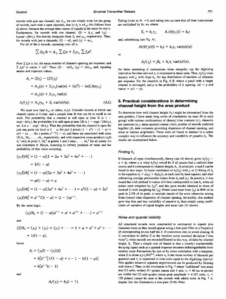
Binomial Transmitter Release
records with just one channel, say A j, we can simply write for the groupof records, each with n open channels, that its Aj is nA Ij; this follows from(i) above, because the average time course of signals is the same for any n.Furthermore, for records with one channel, (S) = hCcT and (yj) =hCexp(-j5t/Tc). For brevity designate these SI and y,j, respectively. Then,for records with just n channels, (S) = nS1 and (yi) = nyj
For all of the k records, summing over all n,
> Syv/k = Aj E>fnn + Slylj Ifnn2.
Now - fnn is (n), the mean number of channels opening per response, andT, f,n2 is var(n) + (n)2. Thus, (S) = (n)S1, (yj) = (n)y,j, and, equatingmeans and expected values,
Ai = (Sy)- (SX(yj)= Aij(n) + S1ylj(var(n) + (n)2) - (nSI)(ny1I)= Alj(n) + Slylj var(n)
Aj/(yj) = A1j/ylj + SI var(n)/(n). (Al)
We must now find A j, or rather, AI (t). Consider records at which onechannel opens at 0 time, and a sample time St that can be as small as wewish. The probability that a channel is still open at time St is 1 -exp(-&t/T'), the probability it is still open at time 2&t is 1 - exp(-25t/Tr),etc. Let a = exp(- Stt/,e). Then the probability that the channel is open forjust one point (or less) is 1 - a, for just 2 points (1 - a2) - (1 - a) =a(1- a), . . . for x points aX-(1 - a), and these are associated with sums(S) hc, 2hc,. xhc, respectively, and with respective cross-products (yiS)hc2 only at point 1, 2hc2 at points 1 and 2 only, . . ., xhc2 for all points 'xand elsewhere 0. Hence, summing to infinity products of value and theprobability of that value occurring,
(y,S)/h=2 (1-a)(l + 2a + 3a2 + 4a3+ )
= 11(1 -a)
(y2S)/hc = (1- a)(2a + 3a2 + 4a3 + .)
= a/(l- a) + a
(y3S)lh2 = (1 - a)(3a2 + 4a3 + ***) = a2/(1 - a) + 2a2
(yiS)lh/2 = ai-1/(1 - a) + (i -1)ai- .
By the same logic,
(yi)/hc = (1 - a)(a'-' + a' + a'+' + ) =
and
= 1/(1 - a),
hence
Ai = (yiS) - (yX)(S)h2ai-[l/(1 - a) + i - 1 - 1/(1 - a)]
h2a'-'(i - 1)
and
Taking limits as St - 3 0, and taking into account that all time summationsare multiplied by St, we obtain
SI = hCTc; Aj(t)/yi(t) = hct
and, substituting into Eq. Al,
A(t)/(y(t)) = hct + hcTc var(n)/(n)
or
Aj/(yj) = ihc + hcTc var(n)/(n),
the latter pertaining if summations (time integrals) use the digitizinginterval as the time unit and Tc is expressed in these units. Thus, Aj/(yj) riseslinearly with j, with slope hc, for any distribution of numbers of channelsper response. For the situation in Fig. 6 B, where a patch with a singlechannel is envisaged, and p is the probability of it opening, (n) = p andvar(n) = p(l - p).
5. Practical considerations in determiningchannel height from the area productTo determine how well channel height (he) might be determined from thearea product, I have made long series of simulations (at least 50 in eachgroup) with various combinations of channel time constant (c), channelsper quantum (nc), mean quantal content ((m)), number of records analyzedtogether (k), time constants governing dispersion of channel opening, andnoise at various amplitudes. These were all found to interact in a rathercomplex way to influence the accuracy and variability of putative hc. Theresults are summarized below.
Finding hc
If channels all open simultaneously, theory (see (4) above) gives Aj/(yj) =a + bj, where a is what Aj/(yj) would be if all quanta had a uniform timecourse and b corresponds to channel height, h,. In principle, a and b can befound in two ways: 1) linear correlation of Aj/(yj) with j, or 2) fitting of Ajto the equation Aj = a(yj) + b(j(yj)), in each case by least squares, and aftersubtracting average prestimulus values from Aj and (yj). In practice, it wasfound that with method 1) values of b best corresponded to true hc when allpoints were weighted by (y)3, and this gave results identical to those ofmethod 2) with weighting by (yj). Points used were from (yj) at 90% of itspeak to 2.5% of its peak, to exclude (most) of the error otherwise arisingfrom (minor) time dispersion of channel opening. Invariably, this methodgave less bias and less variability of putative hc than simply using coeffi-cients of variation of signal heights and areas (see (3) above).
Noise and quantal visibility
All simulated records were constructed to correspond to signals plusGaussian noise as they would appear using a low-pass filter at a frequency(f) corresponding to one-half the A-D conversion rate, to avoid aliasing. Itis convenient to define Z as the baseline noise standard deviation ("rmsnoise"), when records are recorded/filtered in this way, divided by channelheight, hc Then a simple rule of thumb is that a (nearly) exponentiallydecaying signal such as a quantal response becomes indistinguishable fromrandom noise fluctuations by eye or by cross-correlation with a template,when Z is about nc(Tc/80)05, where nc is the mean number of channels perquantum and Tr is expressed in time units equal to the digitizing interval.This applies whatever apparent improvement can be produced by filteringwith lowerf. Thus, in the simulation in Fig. 7 where "unfiltered" rms noisewas 0.5 units, unitary GI quanta (mean size 1 unit, Tc = 40 ms or points)are visible but G2 unit quanta (mean peak amplitude = 0.167 units, TC =120 points) cannot be seen in the records with added noise in Fig. 7 A,despite (for the illustration) a low-pass 25-Hz filter.
751Quastel
Ail(yi) = hc(i 1).

752 Biophysical Journal Volume 72 February 1997
Filtering the mean and area product
Although smoothing individual records was not useful, smoothing of bothA(t) and (y(t)) by simple low-pass filtering before finding b by least squaresled to less variability of b. The time constant for this was chosen as 10%of the apparent time constant by which (yj) decayed from 90% to 10% ofits peak; this had a negligible effect to reduce b (see below). Any furthersmoothing with this or smaller time constants, or using running averages,had a negligible effect.
Uncertainty in hcIn the absence of added noise the standard deviation of b/he (which wasapparently normally distributed) was always within about 20% of the valuegiven by the following empirical formula:
SD0(b/hc) = (1 + 0.75/Tc)[1 + 1.2(ncw)05]/k° 5,
where w = (1-p_ + cv2), cvq being the coefficient of variation of quantalheight. Alternatively, in terms of a, n,,w = a/(hjTc). Thus SD0(bIhc) can bequite appreciable if nc is not fairly small and k is only a few hundred. Forexample, in the simulation in Fig. 7 C (k = 400), with quanta having Tc =40 and p' = 0.33, the variation of b/lh, is about ± 0.2 with nr = 10, and ±0.4 with nc = 50.
In the presence of noise, the standard deviations of blhc fit well to theformula
SD(b/hc) = (Vo + Vj)°5,where VO is [SD0(b/hc)]2, and Vn, within about 30%, is given by
n= (15/k)Z(2+x)wO5(m)-1.25,-0.75Here x = 1.25 exp(-Tcnl/l25). For example, in the simulation for Fig. 7C the noise making G2 quanta invisible raises the SD(b/hc) for these quantafrom 0.13 to 0.16 when nc is 2 and from 0.2 to 0.4 when nc = 10. Thetendency for Vn to increase with reduced Tc results in no gain in accuracyof determining hc by reducing the sampling rate and, with it, the prefilterfrequency (J); in the other direction no gain in accuracy occurred withincreasing sampling rate, to make Tc more than about 40 points.
Systematic error produced by noise
Without noise, b was an unbiased estimator of hc, except (see below) withtime dispersion of channel opening or filtering. However, noise produceda downward bias that was evident when (m) and/or k was low. Empirically:
blhc = exp[-(45O/k)Z2/(ncTc(m))].Thus, for example, with quanta composed of an average of 10 channels, anoise level that just makes individual quanta invisible (Z = 10 if Tr = 80)gives with (m) = 1, blhc = 0.57 at k = 100 and blhe = 0.87 with k = 400;with (m) = 2.5, blhc = 0.80 and 0.96 at k = 100 and 400, respectively.Such error is signaled by the b obtained from using all records togetherbeing higher than the average of b's obtained by analyzing subgroups ofrecords separately.
Systematic error due to filtering or time dispersion
If channels do not all open simultaneously, (Sy(t)) and (y(t)) are convolutedby the time course of channel opening; exponentially distributed lags ofchannel opening with a mean of Td have the same effect as a low-pass filterwith time constant Td applied to the records. For any particular "filter"(including, for example, electrotonic conduction) the net effect can becalculated by setting up theoretical Aj's and (yj)'s, calculating (Sy-)'s,convoluting the two latter by the appropriate function, and recalculating theresulting As's and Aj/(yj)'s. Using this method or simulation with time-
dispersed channel opening (with up to three time constants) gave the sameresults:
1. Effects to reduce b are less than 2% if the largest time constant, Td,is less than about 20% of T,. Thus, in Fig. 7 C, where quanta of both GI(T = 40) and G2 (T; = 120) type were assumed released with lag timeconstants of 2 and 4.5 points, and channel opening had mean lags of 4 msand 20 ms respectively, these parameters could be expected to have littleeffect on b.
2. With higher Td the graph of Aj/(yj) versus j becomes curvilinear,curving upward to a slope of hc when Td < TC and curving down to a slopeof 0 when Td > TC With b determined as described above (fitting to a linearrelation that is no longer true), blhe averages 0.86 at Td/Tc = 0.5, 0.68 atTd/TC = 0.75, and 0.5 at Td = Ti; with higher Td' b/he declines approximatelye-fold for each increment of Td by T;.
This work was supported by a grant from the Muscular Dystrophy Asso-ciation of Canada.
REFERENCES
Abdul-Ghani, M. A., and P. S. Pennefather. 1993. Sr2' afterdischarge andquantal analysis of synaptic transmission between pairs of culturedmouse hippocampal neurons. Biophys. J. 64:A236.
Bain, A. I., and D. M. J. Quastel. 1992a. Quantal transmitter releasemediated by strontium at the mouse motor nerve terminal. J. Physiol.(Lond.). 450:63-87.
Bain, A. I., and D. M. J. Quastel. 1992b. Multiplicative and additiveCa2+-dependent components of facilitation at mouse endplates.J. Physiol. (Lond.). 455:383-405.
Brown, T. H., D. H. Perkel, and M. W. Feldman. 1976. Evoked neuro-transmitter release: statistical effects of nonuniformity and nonstation-arity. Proc. Natl. Acad. Sci. USA. 73:2913-2917.
del Castillo, J., and B. Katz. 1954a. Quantal components of the end-platepotential. J. Physiol. (Lond.). 124:560-573.
del Castillo, J., and B. Katz. 1954b. Statistical factors involved in neuro-muscular facilitation and depression. J. Physiol. (Lond.). 124:574-585.
del Castillo, J., and B. Katz. 1956. Biophysical aspects of neuro-musculartransmission. Prog. Biophys. 6:121-170.
Dityatev, A. E., V. M. Kozhanov, and S. 0. Gapanovich. 1992. Modelingof the quantal release at intemeuronal synapses: analysis of permissiblevalues of model moments. J. Neurosci. Methods. 43:201-214.
Elmqvist, D., and D. M. J. Quastel. 1965. A quantitative study of end-platepotentials in isolated human muscle. J. Physiol. (Lond.). 178:505-529.
Hubbard, J. I. 1963. Repetitive stimulation at the mammalian neuromus-cular junction and the mobilisation of transmitter. J. Physiol. (Lond.).169:641-662.
Jack, J. J. B., A. U. Larkman, G. Major, and K. J. Stratford. 1994. Quantalanalysis of the synaptic excitation of CAl hippocampal pyramidal cells.In Molecular and Cellular Mechanisms of Neurotransmitter Release. L.Stjarne, P. Greengard, S. E. Grillner, T. G. M. Hokfelt, and D. R.Ottoson, editors. Raven Press, New York.
Katz, B., and R. Miledi. 1965. The measurement of synaptic delay and thetime course of acetylcholine release at the neuromuscular junction. Proc.R. Soc. Lond. B. 161:483-495.
Korn, H., and D. S. Faber. 1991. Quantal analysis and synaptic efficacy inthe CNS. Trends Neurosci. 14:439-445.
Luscher, H. R. 1990. Transmission failure and its relief in the spinalmonosynaptic reflex arc. In The Segmental Motor System. M. D. Binderand L. M. Mendell, editors. Oxford University Press, New York.328-348.
Liley, A. W., and K. A. K. North. 1953. An electrical investigation ofeffects of repetitive stimulation on mammalian neuromuscular junctions.J. Neurophysiol. 16:509-527.
Martin, A. R. 1955. A further study of the statistical composition of theend-plate potential. J. Physiol. (Lond.). 130:114-122.
McLachlan, E. M. 1978. The statistics of transmitter release at chemicalsynapses. In International Review of Physiology, Neurophysiology IHI,Vol. 17. R. Porter, editor. University Park Press, Baltimore. 49-117.

Quastel Binomial Transmitter Release 753
Melkonian, D. S. 1993. Transient analysis of a chemical synaptic trans-mission. Biol. Cybern. 68:341-350.
Mennerick, S., and C. F. Zorumski. 1995. Paired-pulse modulation of fastexcitatory synaptic currents in microcultures of rat hippocampal neu-rons. J. Physiol. (Lond.). 488:85-101.
Mennerick, S., and C. F. Zorumski. 1996. Postsynaptic modulation ofNMDA synaptic currents in rat hippocampal microcultures by paired-pulse stimulation. J. Physiol. (Lond.). 490:405-417.
Press, W. H., S. A. Teukolsky, W. T. Vetterling, and B. P. Flannery. 1992.Numerical Recipes in C, 2nd ed. Cambridge University Press.
Quastel, D. M. J., Y.-Y. Guan, and D. A. Saint. 1992. The relation betweentransmitter release and Ca2+ entry at the mouse neuromuscular junction:
role of stochastic factors causing heterogeneity. Neuroscience. 51:657-67 1.
Redman, S. 1990. Quantal analysis of synaptic potentials in neurons ofcentral nervous system. Physiol. Rev. 70:165-198.
Vere-Jones, D. 1966. Simple stochastic models for the release of quanta oftransmitter from a nerve terminal. Aust. J. Statist. 8:53-63
Walmsley, B. 1993. Quantal analysis of synaptic transmission. InElectrophysiology: A Practical Approach. D. I. Wallis, editor. IRL Press,Oxford.
Weatherburn, C. E. 1961. A First Course in Mathematical Statistics.Cambridge University Press, Cambridge.