the basics of r - lu filegeorg krammer the basics ofr 3 1) introduction 2) basics 3) descriptive...
TRANSCRIPT

Georg Krammer The Basics of R 1
The Basics of R
Georg Krammer The Basics of R 2
Wednesday, 18.05.2016 09:00 – 12:00: R 12:00 – 13:00: Lunch 13:00 – 16:00: R
Thursday, 19.05.2016 09:00 – 12:00: R 12:00 – 13:00: Lunch 13:00 – 16:00: R
Schedule
Georg Krammer The Basics of R 3
1) Introduction2) Basics3) Descriptive statistics4) t‐tests5) Correlations
Contents
Help you, to help yourself!

Georg Krammer The Basics of R 4
Why use R?
Luhmann (2011):R can do more. Within R, many functions are implemented that commercial statisticssoftwares such as SPSS lack. R is fast‐paced.R is constantly being developed. Many statistical methods are first implentedin R, before being implemented years later in other softwares. R is approachable and responsive. All the programers of the package are usually reachable via e‐mail and will respond. Thus, questions can often be clarified very easily, and possible bugsfound and fixed. R is free!
Introduction

Georg Krammer The Basics of R 5
Introduction: graphical example1) The α level

Georg Krammer The Basics of R 6
Introduction: graphical example1) The α level
Georg Krammer The Basics of R 7
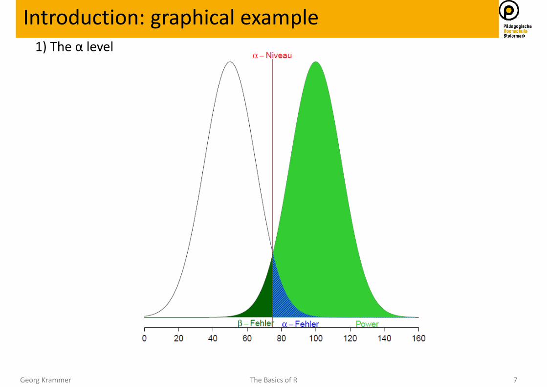
Introduction: graphical example1) The α level
Georg Krammer The Basics of R 8
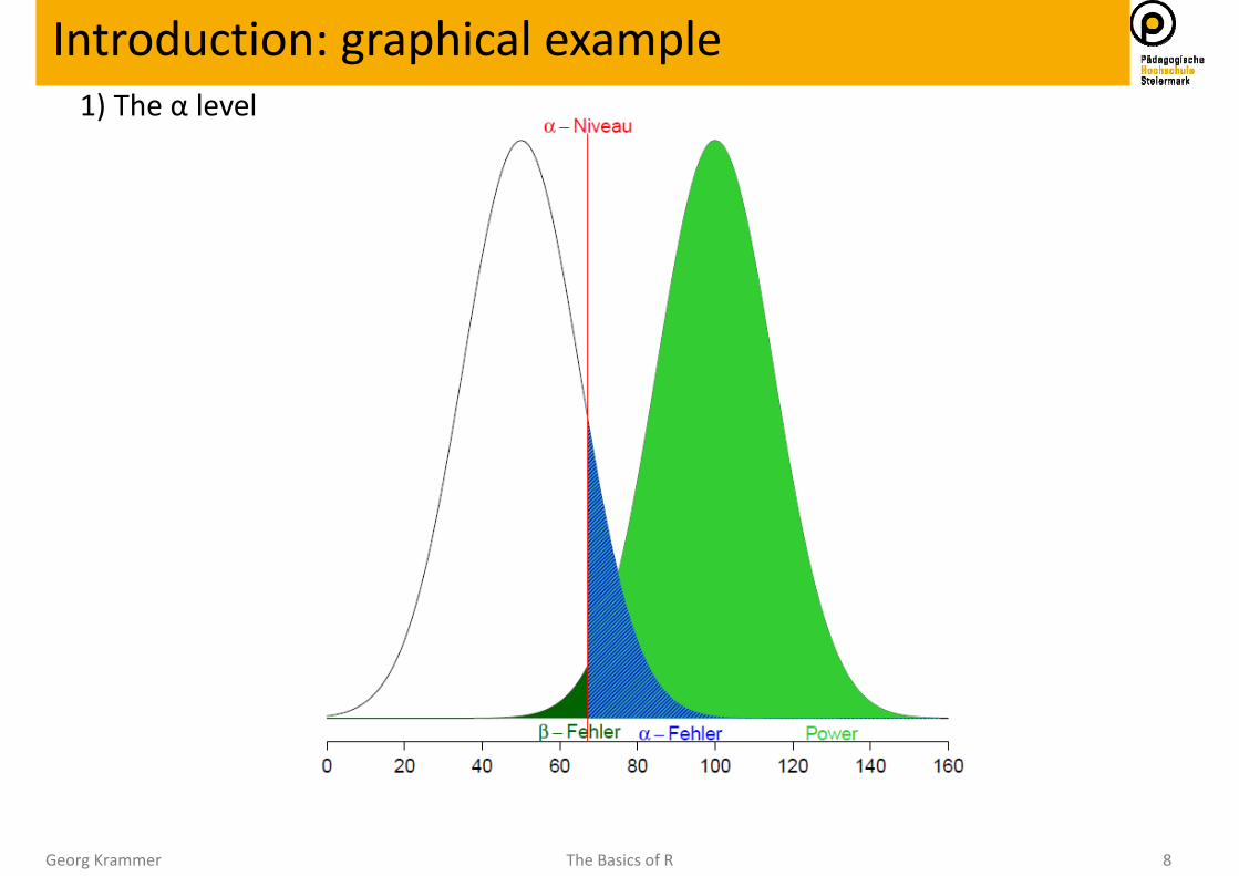
Introduction: graphical example1) The α level

Georg Krammer The Basics of R 9
Introduction: graphical example1) The α level
α = .01
α = .10 α = .25
α = .05
Georg Krammer The Basics of R 10
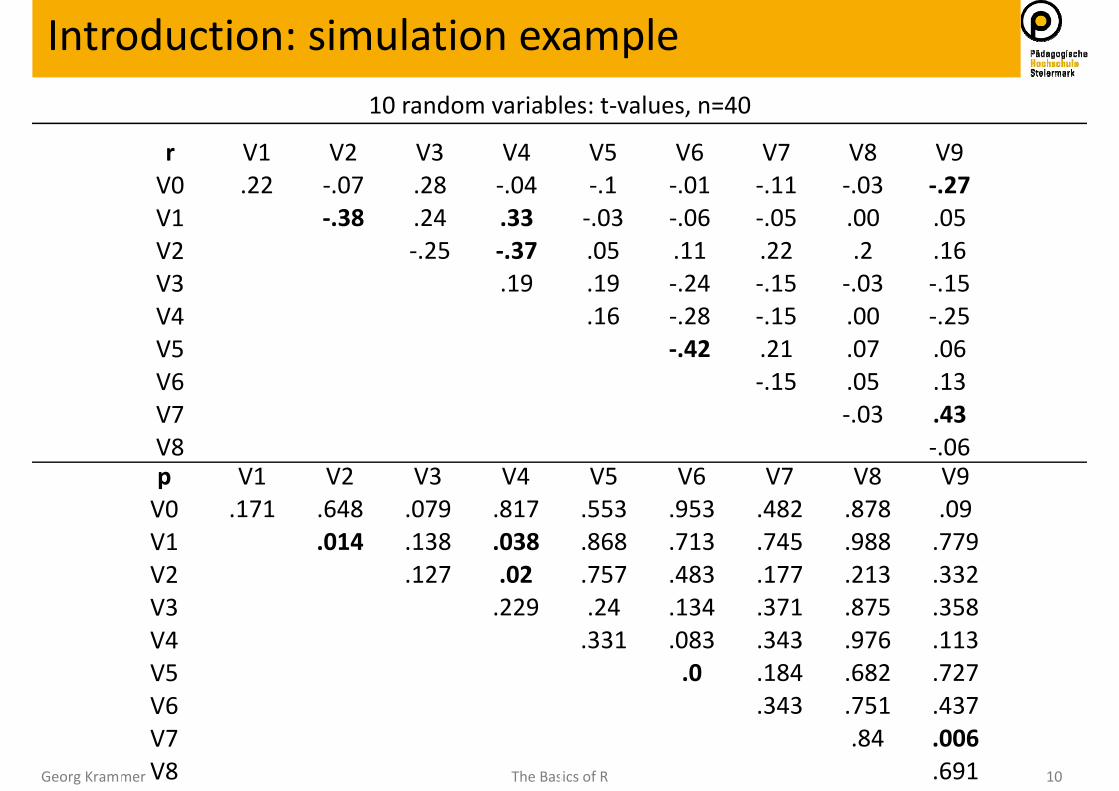
r V1 V2 V3 V4 V5 V6 V7 V8 V9V0 .22 ‐.07 .28 ‐.04 ‐.1 ‐.01 ‐.11 ‐.03 ‐.27V1 ‐.38 .24 .33 ‐.03 ‐.06 ‐.05 .00 .05V2 ‐.25 ‐.37 .05 .11 .22 .2 .16V3 .19 .19 ‐.24 ‐.15 ‐.03 ‐.15V4 .16 ‐.28 ‐.15 .00 ‐.25V5 ‐.42 .21 .07 .06V6 ‐.15 .05 .13V7 ‐.03 .43V8 ‐.06
Introduction: simulation example
p V1 V2 V3 V4 V5 V6 V7 V8 V9V0 .171 .648 .079 .817 .553 .953 .482 .878 .09V1 .014 .138 .038 .868 .713 .745 .988 .779V2 .127 .02 .757 .483 .177 .213 .332V3 .229 .24 .134 .371 .875 .358V4 .331 .083 .343 .976 .113V5 .0 .184 .682 .727V6 .343 .751 .437V7 .84 .006V8 .691
10 random variables: t‐values, n=40

Georg Krammer The Basics of R 11
10 random variablest‐valuesn=401000 repetitions
For the correlations of all the 1000 repetitions: M: .000391055 .000 (SD: .02434984) .024 Minimum M: ‐.05975123 ‐.060 Maximum M: .1129733 .110
Highest correlation: ± .6552521 ± .655 Lowest correlation: .0000004 .000
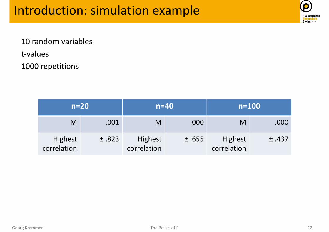
Introduction: simulation example
Georg Krammer The Basics of R 12
10 random variablest‐values1000 repetitions
Introduction: simulation example
n=20 n=40 n=100
M .001 M .000 M .000
Highestcorrelation
± .823 Highestcorrelation
± .655 Highestcorrelation
± .437
Georg Krammer The Basics of R 13
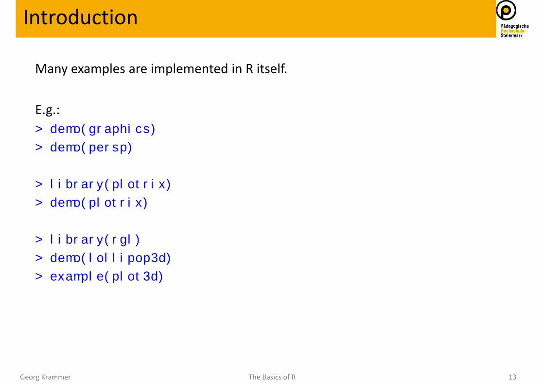
Many examples are implemented in R itself.
E.g.: > demo(graphics)
> demo(persp)
> library(plotrix)
> demo(plotrix)
> library(rgl)
> demo(lollipop3d)
> example(plot3d)
Introduction
Georg Krammer The Basics of R 14
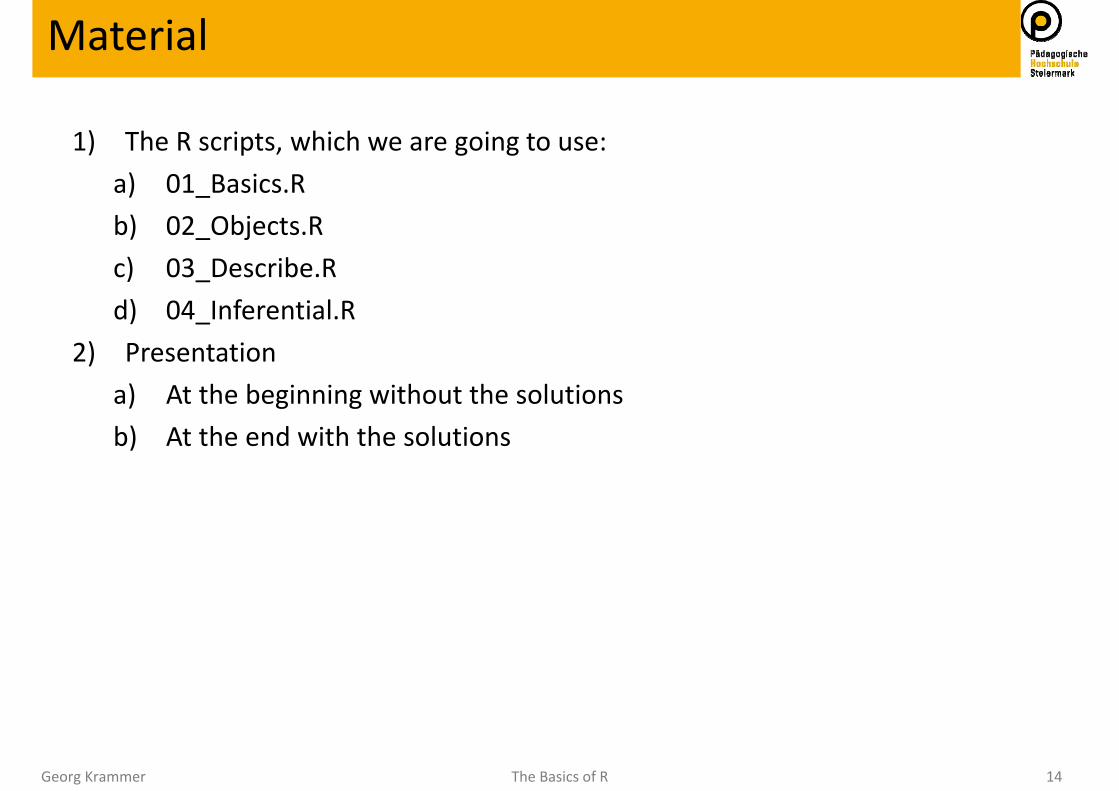
1) The R scripts, which we are going to use:a) 01_Basics.Rb) 02_Objects.Rc) 03_Describe.Rd) 04_Inferential.R
2) Presentationa) At the beginning without the solutionsb) At the end with the solutions
Material

Georg Krammer The Basics of R 15
1) R (http://cran.at.r‐project.org/) and2) RStudio (http://www.rstudio.com/ide/download/).
Introduction
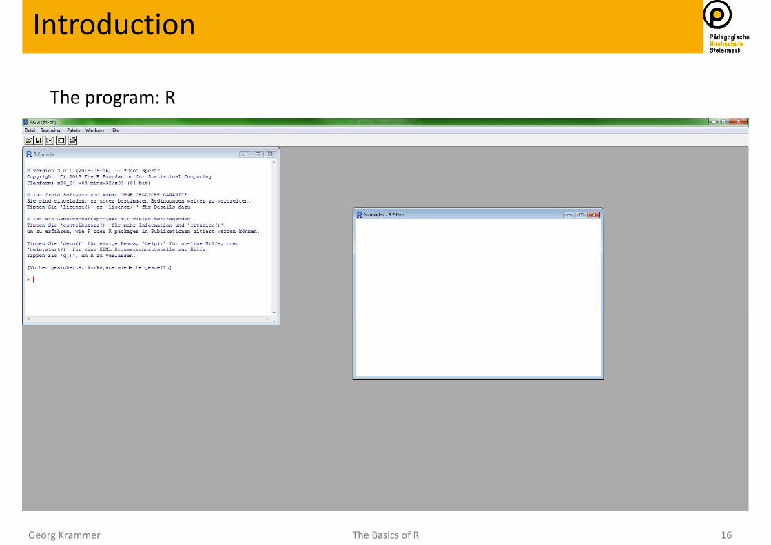
The R Project for Statistical Computing The program itself
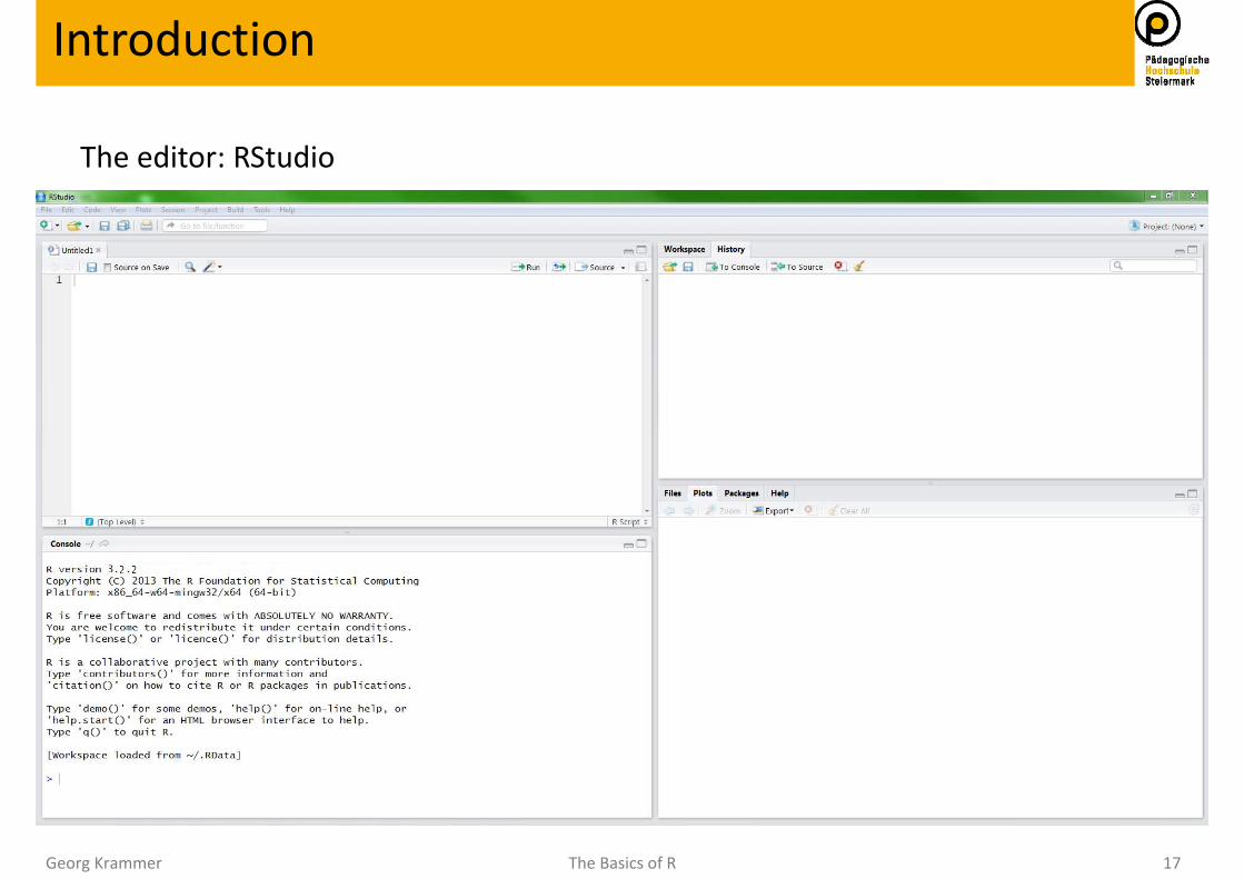
RStudio An editor to make life a lot easier
Georg Krammer The Basics of R 16
The program: R
Introduction
Georg Krammer The Basics of R 17
The editor: RStudio
Introduction

Georg Krammer The Basics of R 18
no syntax highlighting
Introduction
vs. syntax highlighting

Georg Krammer The Basics of R 19
Introduction
Script
Console
Workspace,history
Files,plots,packages,help

Georg Krammer The Basics of R 20
Essentially, R is easy to handle …sometime you just need to know where tolook things up.
Introduction
Georg Krammer The Basics of R 21
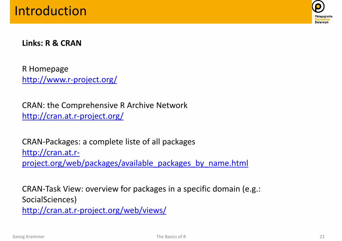
Links: R & CRAN
R Homepagehttp://www.r‐project.org/
CRAN: the Comprehensive R Archive Networkhttp://cran.at.r‐project.org/
CRAN‐Packages: a complete liste of all packageshttp://cran.at.r‐project.org/web/packages/available_packages_by_name.html
CRAN‐Task View: overview for packages in a specific domain (e.g.: SocialSciences) http://cran.at.r‐project.org/web/views/
Introduction
Georg Krammer The Basics of R 22
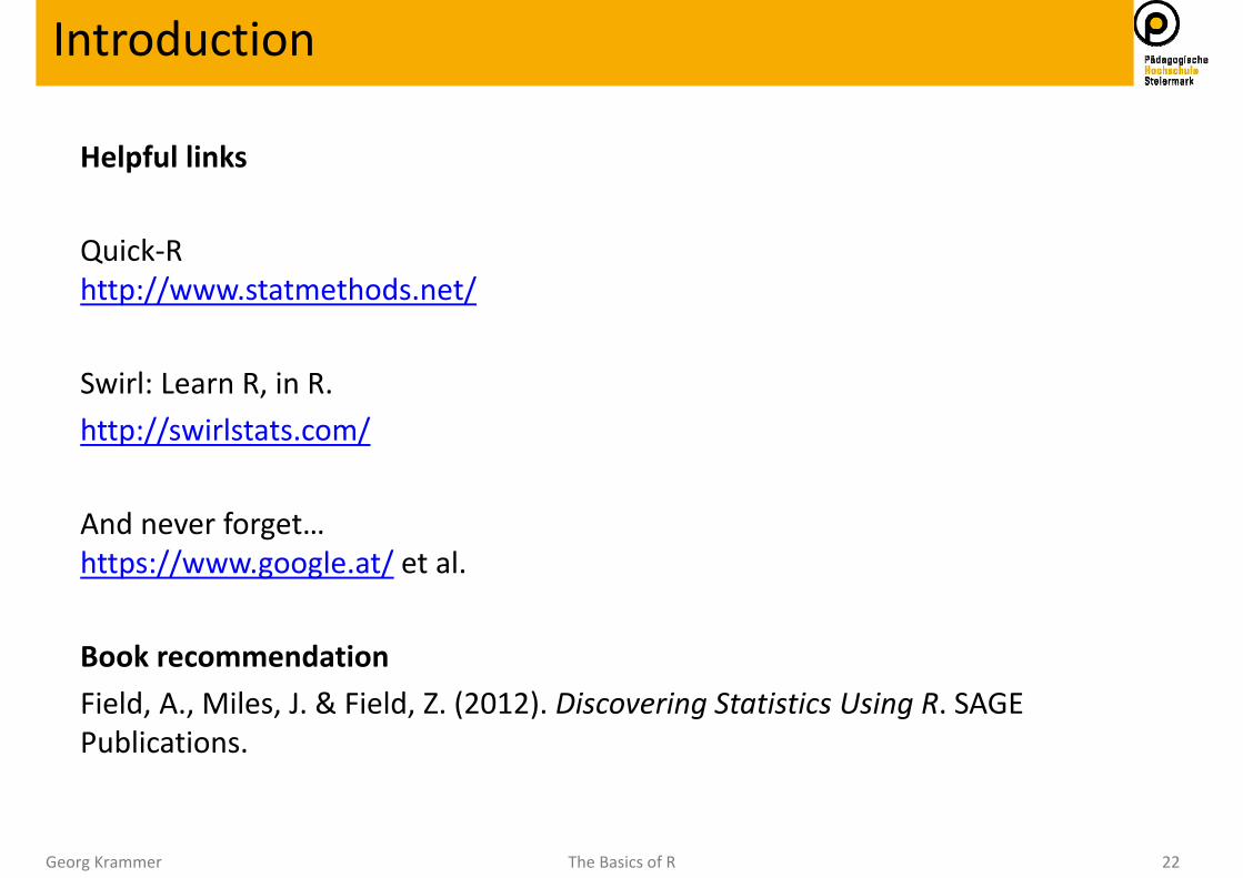
Helpful links
Quick‐Rhttp://www.statmethods.net/
Swirl: Learn R, in R.http://swirlstats.com/
And never forget…https://www.google.at/ et al.
Book recommendationField, A., Miles, J. & Field, Z. (2012). Discovering Statistics Using R. SAGE Publications.
Introduction

Georg Krammer The Basics of R 23
References
Field, A., Miles, J. & Field, Z. (2012). Discovering Statistics Using R. SAGE Publications.
Introduction
Georg Krammer The Basics of R 24
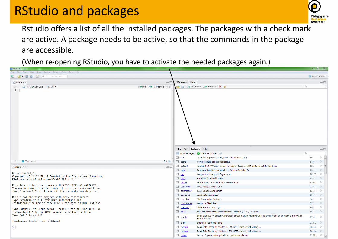
Rstudio offers a list of all the installed packages. The packages with a check markare active. A package needs to be active, so that the commands in the packageare accessible. (When re‐opening RStudio, you have to activate the needed packages again.)
RStudio and packages
Georg Krammer The Basics of R 25
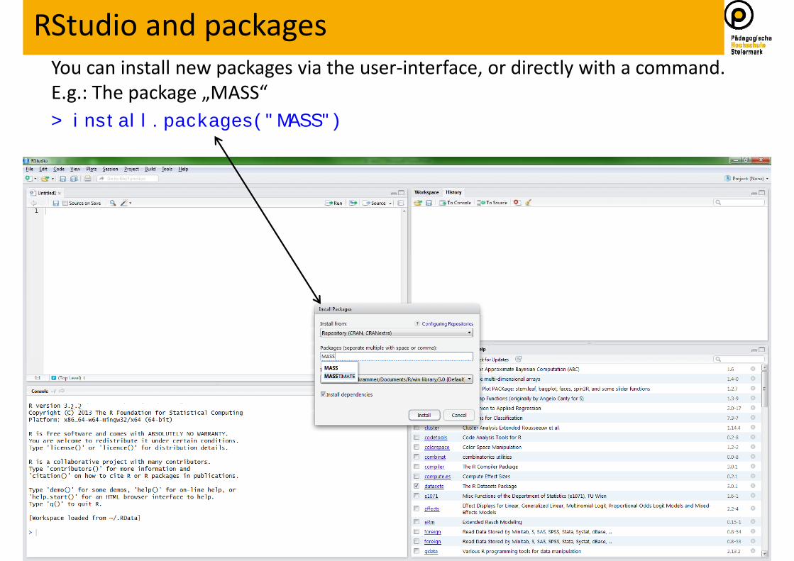
You can install new packages via the user‐interface, or directly with a command. E.g.: The package „MASS“> install.packages("MASS")
RStudio and packages
Georg Krammer The Basics of R 26
RStudio and packages
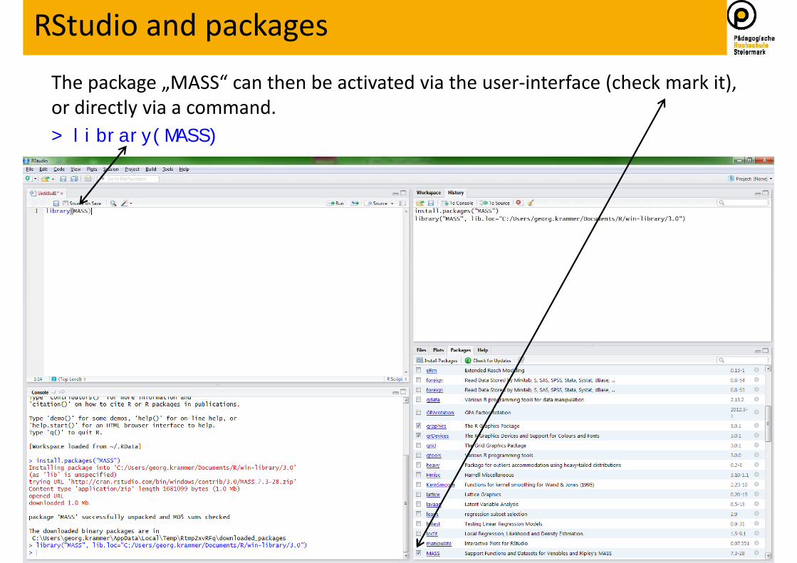
The package „MASS“ can then be activated via the user‐interface (check mark it), or directly via a command. > library(MASS)
Georg Krammer The Basics of R 27
Clicking on the name of a package opens the corresponding help page. There, you can find the complete documentation of the package, as well as a complete list of all commands within the package.
> help(command)
opens the help page of a command. This will not work, if the command is not recognised (e.g. misspelled, or in a package that is currently not active). Pressing „F1“ in RStudio does the same (to do so, click on the command in your script and press „F1“).
> ??command
browses through all help sites. This way, you can find commands of not activepackages, not installed packages, or even incomplete commands. The search bar in the Help tap in RStudio does the same.
RStudio and help

Georg Krammer The Basics of R 28
It costs nothing to ask!Usually, commands work with many different arguments. It is not necessaryto know each and every command and argument by heart.
> help(command)
> ??command
RStudio and help
Georg Krammer The Basics of R 29
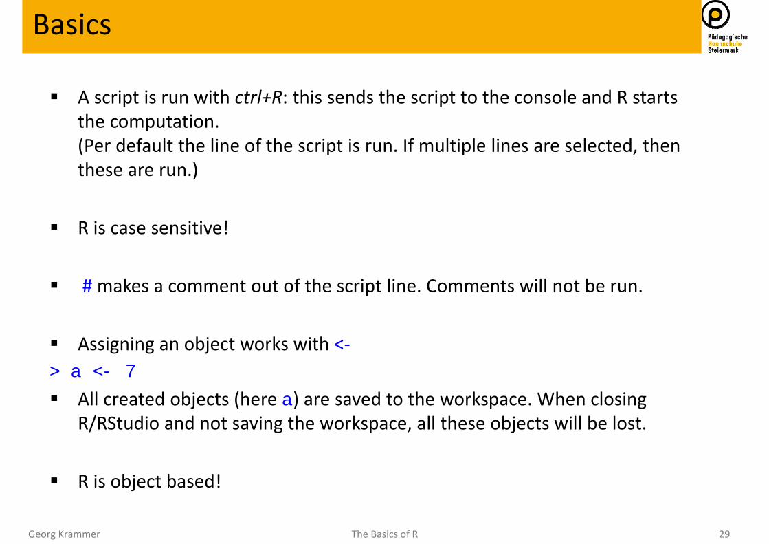
A script is run with ctrl+R: this sends the script to the console and R startsthe computation. (Per default the line of the script is run. If multiple lines are selected, thenthese are run.)
R is case sensitive!
# makes a comment out of the script line. Comments will not be run.
Assigning an object works with <‐> a <- 7
All created objects (here a) are saved to the workspace. When closingR/RStudio and not saving the workspace, all these objects will be lost.
R is object based!
Basics
Georg Krammer The Basics of R 30
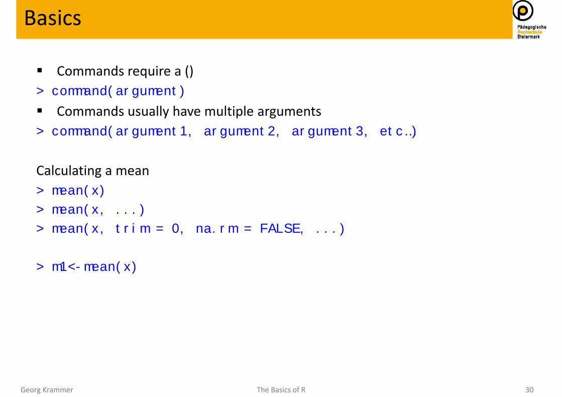
Commands require a () > command(argument)
Commands usually have multiple arguments> command(argument1, argument2, argument3, etc…)
Calculating a mean> mean(x)
> mean(x, ...)
> mean(x, trim = 0, na.rm = FALSE, ...)
> m1<-mean(x)
Basics
Georg Krammer The Basics of R 31
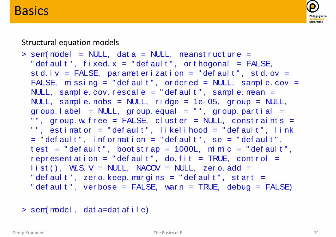
Structural equation models> sem(model = NULL, data = NULL, meanstructure = "default", fixed.x = "default", orthogonal = FALSE, std.lv = FALSE, parameterization = "default", std.ov = FALSE, missing = "default", ordered = NULL, sample.cov = NULL, sample.cov.rescale = "default", sample.mean = NULL, sample.nobs = NULL, ridge = 1e-05, group = NULL, group.label = NULL, group.equal = "", group.partial = "", group.w.free = FALSE, cluster = NULL, constraints = '', estimator = "default", likelihood = "default", link = "default", information = "default", se = "default", test = "default", bootstrap = 1000L, mimic = "default", representation = "default", do.fit = TRUE, control = list(), WLS.V = NULL, NACOV = NULL, zero.add = "default", zero.keep.margins = "default", start = "default", verbose = FALSE, warn = TRUE, debug = FALSE)
> sem(model, data=datafile)
Basics
Georg Krammer The Basics of R 32
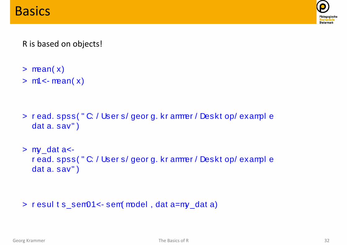
R is based on objects!
> mean(x)
> m1<-mean(x)
> read.spss("C:/Users/georg.krammer/Desktop/example data.sav")
> my_data<-read.spss("C:/Users/georg.krammer/Desktop/example data.sav")
> results_sem01<-sem(model,data=my_data)
Basics
Georg Krammer The Basics of R 33
Basics
01_Basics.R
Georg Krammer The Basics of R 34
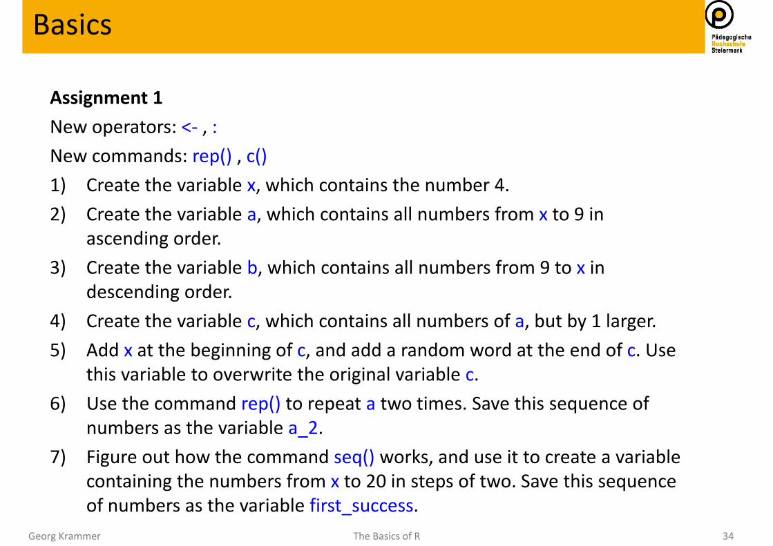
Assignment 1New operators: <‐ , :New commands: rep() , c()1) Create the variable x, which contains the number 4. 2) Create the variable a, which contains all numbers from x to 9 in
ascending order. 3) Create the variable b, which contains all numbers from 9 to x in
descending order. 4) Create the variable c, which contains all numbers of a, but by 1 larger. 5) Add x at the beginning of c, and add a random word at the end of c. Use
this variable to overwrite the original variable c.6) Use the command rep() to repeat a two times. Save this sequence of
numbers as the variable a_2.7) Figure out how the command seq() works, and use it to create a variable
containing the numbers from x to 20 in steps of two. Save this sequenceof numbers as the variable first_success.
Basics
Georg Krammer The Basics of R 36
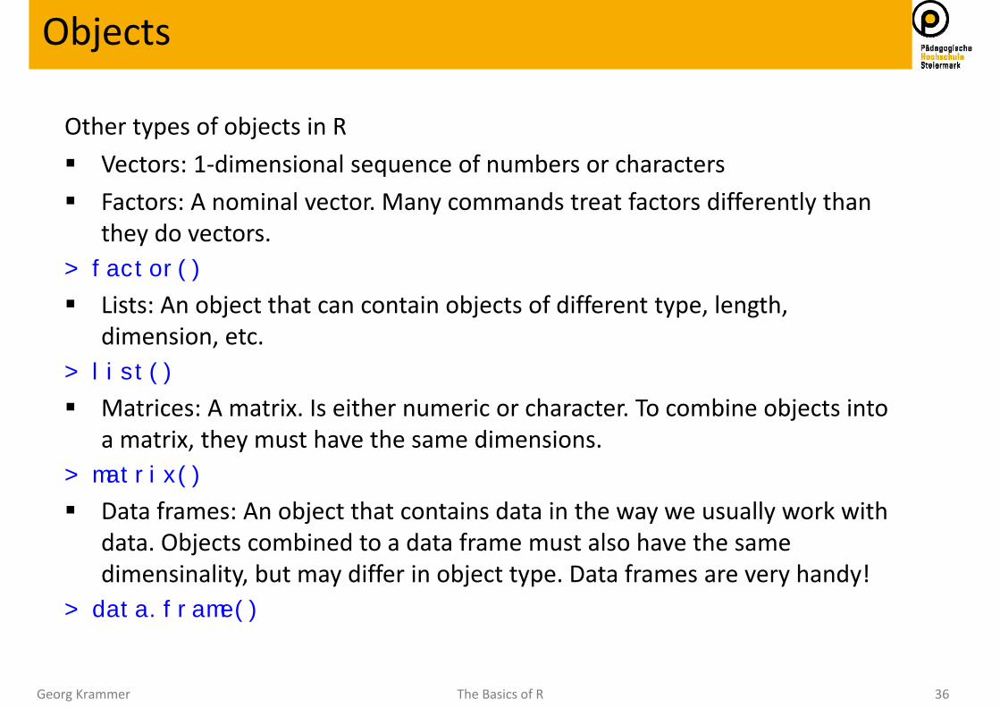
Other types of objects in R Vectors: 1‐dimensional sequence of numbers or characters Factors: A nominal vector. Many commands treat factors differently than
they do vectors. > factor()
Lists: An object that can contain objects of different type, length, dimension, etc.
> list()
Matrices: A matrix. Is either numeric or character. To combine objects intoa matrix, they must have the same dimensions.
> matrix()
Data frames: An object that contains data in the way we usually work withdata. Objects combined to a data frame must also have the same dimensinality, but may differ in object type. Data frames are very handy!
> data.frame()
Objects

Georg Krammer The Basics of R 37
Objects
02_Objects.R

Georg Krammer The Basics of R 38
Assignment 2New commands: factor(), list(), matrix(), data.frame(), as.data.frame(),length(), rbind(), cbind(), dim(), ncol(), nrow(), colnames(), rownames()1) Create the variable a, which containts the numbers 5, 8, 5, 10, 4, 9, 8, 1,
8, 3. 2) Create the variable b, which contains the letters “b“, “c“, “b“, “a“, “a“, “a“,
“b“, “a“, “a“, “a“. 3) Create the matrix m1, wherein a and b are the columns. 4) Create the data frame d1 out of m1. 5) Add a column to d1, which states that the subjects in the top half of all
the rows were in the control group, and that the second half was in thetreatment group. (Watch out that d1 remains a data frame)
6) Rename the columns of d1, so that the columns „a“ and „b“ are nowcalled „dv1“ and „dv2“, and the last column „iv“.
7) Create the list l, which contains the dimension, the column names, andthe row names of d1.
Objects

Georg Krammer The Basics of R 40
Objects
Back to 02_Objects.R

Georg Krammer The Basics of R 41
Assignment 3New operators: ==, !=, <, >, <=, >=, &, |, [], $New commands: subset(), str(), ls(), attributes()1) Create the matrix m, which has 10 columns and 4 rows, and contains
numbers in ascending order, beginning with 2. 2) Create a data frame from m, and with it overwrite the variable m.3) Rename the columns of m into „t1“, „t2“, „t3“, and „t4“. 4) Create the object x1, which only contains the first two columns of m. 5) Create the object x2, which only contains the last two rows of m. 6) Multiply x1 with the number in the 4th column and 9th row of m. 7) Create the object x3, which only contains the rows of m, where t1 was
greater than 8. 8) Create the object x4, which contains only the values of t4, where t1 was
greater than 8.
Objects
Georg Krammer The Basics of R 43
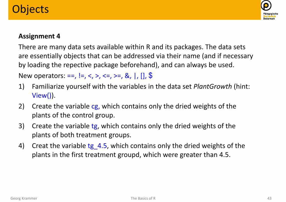
Assignment 4There are many data sets available within R and its packages. The data setsare essentially objects that can be addressed via their name (and if necessaryby loading the repective package beforehand), and can always be used. New operators: ==, !=, <, >, <=, >=, &, |, [], $1) Familiarize yourself with the variables in the data set PlantGrowth (hint:
View()). 2) Create the variable cg, which contains only the dried weights of the
plants of the control group. 3) Create the variable tg, which contains only the dried weights of the
plants of both treatment groups. 4) Creat the variable tg_4.5, which contains only the dried weights of the
plants in the first treatment groupd, which were greater than 4.5.
Objects
Georg Krammer The Basics of R 45
Descriptive Statistics
1. Find x
Georg Krammer The Basics of R 46
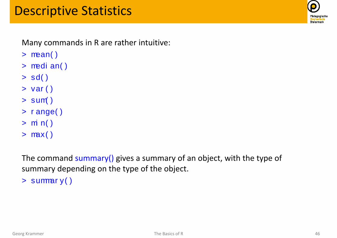
Many commands in R are rather intuitive:> mean()
> median()
> sd()
> var()
> sum()
> range()
> min()
> max()
The command summary() gives a summary of an object, with the type of summary depending on the type of the object. > summary()
Descriptive Statistics

Georg Krammer The Basics of R 47
Descriptive Statistics
03_Describe.R

Georg Krammer The Basics of R 48
Assignment 5New commands: mean(), sd(), etc…; summary(), hist(), boxplot(), barplot(),apply(), sapply() 1) Do whatever is necessary to make the data set cats available for you. 2) Familiarize yourself with the variables in the data set cats. 3) Plot a histogram for the body weight and the heart weight of the
domestic cats, and plot a boxplot for both. 4) Create the vector v_kg, which contains the mean, the standard deviation,
the minimum, and the maximum of the domestic cats‘ body weight. 5) Create the vector v_hg, which contains the mean, the standard deviation,
the minimum, and the maximum of the domestic cats‘ heart weight. 6) Combine v_kg and v_hg to the data frame kitties and label it
meaningfully.
Descriptive Statistics
Georg Krammer The Basics of R 50
Descriptive Statistics
Back to 03_Describe.R
Georg Krammer The Basics of R 51
Assignment 6New operators: ~, *New commands: tapply(), by(), aggregate()1) Do whatever is necessary to make the data set HolzingerSwineford1939
available for you. 2) Familiarize yourself with the variables in the data set HolzingerSwineford1939
(hint: View(HolzingerSwineford1939)).3) Create the variable vw_all, which contains the mean and the standard
deviation of the visual perception. 4) Create one boxplot to visualize the mean visual perception of the genders and
types of schools. 5) Create the object vw_school_gender, which contains the means and standard
deviations of the visual perception seperately for the genders and types ofschools.
6) Optional: solve 5) in a different way.
Descriptive Statistics
Georg Krammer The Basics of R 56
Descriptive Statistics
Georg Krammer The Basics of R 57
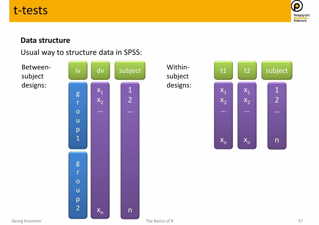
Data structureUsual way to structure data in SPSS:
t‐tests
group1
x1x2…
xn
group2
iv dv
x1x2…
xn
t1 t2
x1x2…
xn
Between‐subjectdesigns:
Within‐subjectdesigns:
subject
12…
n
subject
12…
n
Georg Krammer The Basics of R 58
x1x2…
xn
x1x2…
xn
12…
n
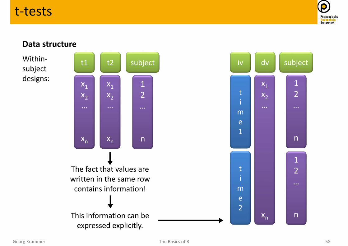
Data structure
t‐tests
t1 t2Within‐subjectdesigns:
subject
12…
n
The fact that values arewritten in the same rowcontains information!
This information can beexpressed explicitly.
subject
12…
n
12…
n
time1
x1x2…
xn
time2
iv dv
x1x2…
xn
x1x2…
xn
12…
n

Georg Krammer The Basics of R 59
Data structureGeneral way of structuring data:
t‐tests
group1
x1x2…
xn
group2
iv dvBetween‐subjectdesigns:
Within‐subjectdesigns:
subject
12…
n
subject
12…
n
12…
n
time1
x1x2…
xn
time2
iv dv
Georg Krammer The Basics of R 60
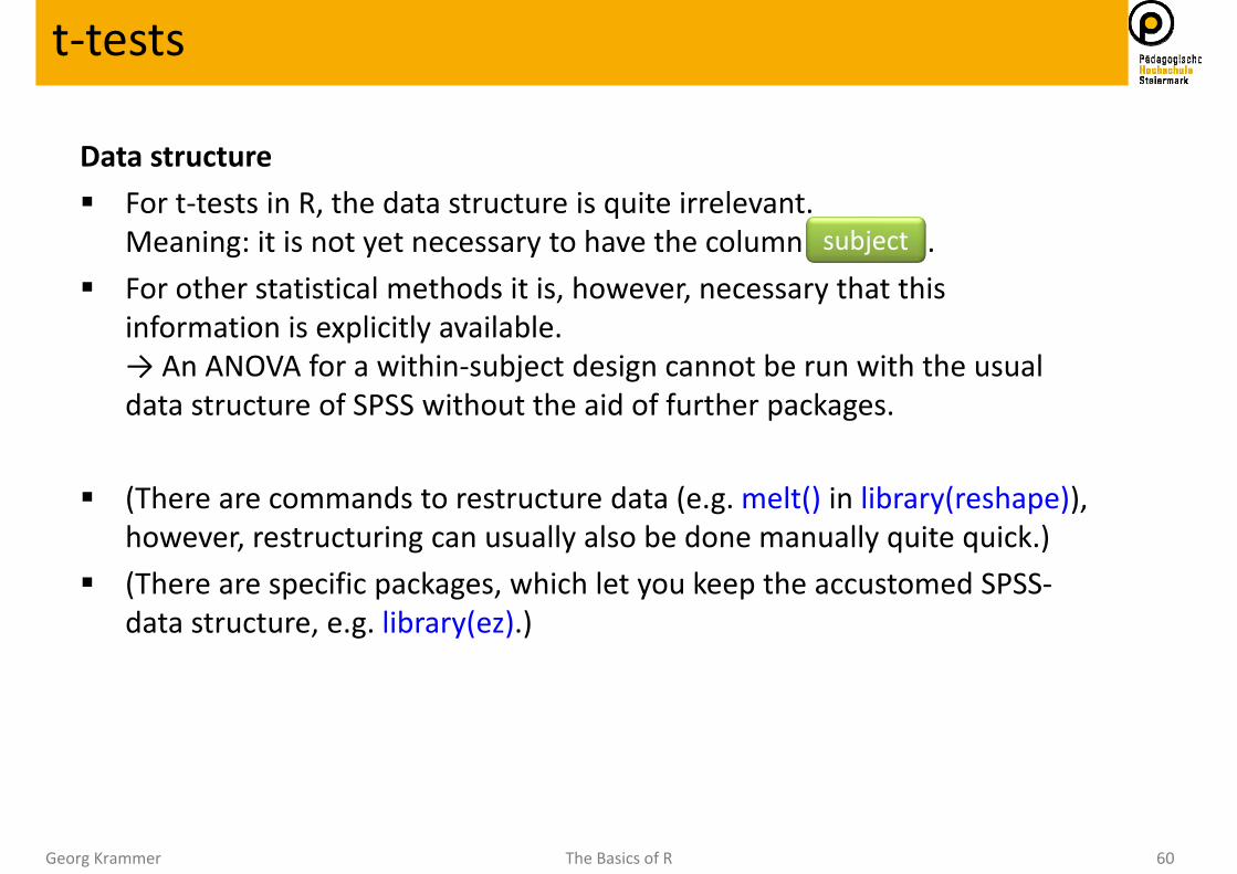
Data structure For t‐tests in R, the data structure is quite irrelevant.
Meaning: it is not yet necessary to have the column . For other statistical methods it is, however, necessary that this
information is explicitly available. → An ANOVA for a within‐subject design cannot be run with the usualdata structure of SPSS without the aid of further packages.
(There are commands to restructure data (e.g. melt() in library(reshape)), however, restructuring can usually also be done manually quite quick.)
(There are specific packages, which let you keep the accustomed SPSS‐data structure, e.g. library(ez).)
t‐tests
subject

Georg Krammer The Basics of R 61
t.test() The command for all t‐tests is t.test(). t.test() can be used with a formula, t.test(dv ~ iv), or with two objects
containing the data of the two groups, t.test(x,y). Per default, t.test() computes independent sample t‐tests. For a
dependent sample t‐test, t.test() needs to be told in an argument that thedata is dependent.
> t.test(…, paired=TRUE).
This hold when you are using formulas, and when not: independent: dependent:
Per default, t.test() assumes the variances to be unequal.
t‐tests
>t.test(dv ~ iv) ↔ >t.test(x,y)
>t.test(dv ~ iv,paired=T) ↔ >t.test(x,y,paired=T)
Georg Krammer The Basics of R 62
t‐tests
04_Inferential.R

Georg Krammer The Basics of R 63
Assignment 7New command: t.test()Answer the following questions with the data set iris.
Solve 1) and 2) first without, and then with using a formula. 1) Do the species of iris virginica and versicolor differ in their mean petal
lengths?2) Do the irises differ in the length of their petals and sepals?
t‐tests

Georg Krammer The Basics of R 65
Correlations
Back to 04_Inferential.R
Georg Krammer The Basics of R 66
Assignment 8New commands: cor(), cor.test(), rcorr()Use the data set HolzingerSwineford1939 for the following. 1) Calculate the pearson‐correlation, and the spearman‐correlation
between the exact age of the children and their performance in thevisual perception task.
2) Test the correlations of 1) for their significance. 3) Calculate the intercorrelations of the performance measures. 4) Calculate the intercorrelations of the performance measures only for the
children of the pasteur‐school.
Correlations
Georg Krammer The Basics of R 68
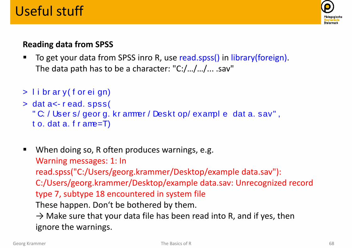
Reading data from SPSS To get your data from SPSS inro R, use read.spss() in library(foreign).
The data path has to be a character: "C:/…/…/... .sav"
> library(foreign)
> data<-read.spss("C:/Users/georg.krammer/Desktop/example data.sav",to.data.frame=T)
When doing so, R often produces warnings, e.g.Warning messages: 1: In read.spss("C:/Users/georg.krammer/Desktop/example data.sav"): C:/Users/georg.krammer/Desktop/example data.sav: Unrecognized recordtype 7, subtype 18 encountered in system fileThese happen. Don‘t be bothered by them. → Make sure that your data file has been read into R, and if yes, thenignore the warnings.
Useful stuff
Georg Krammer The Basics of R 69
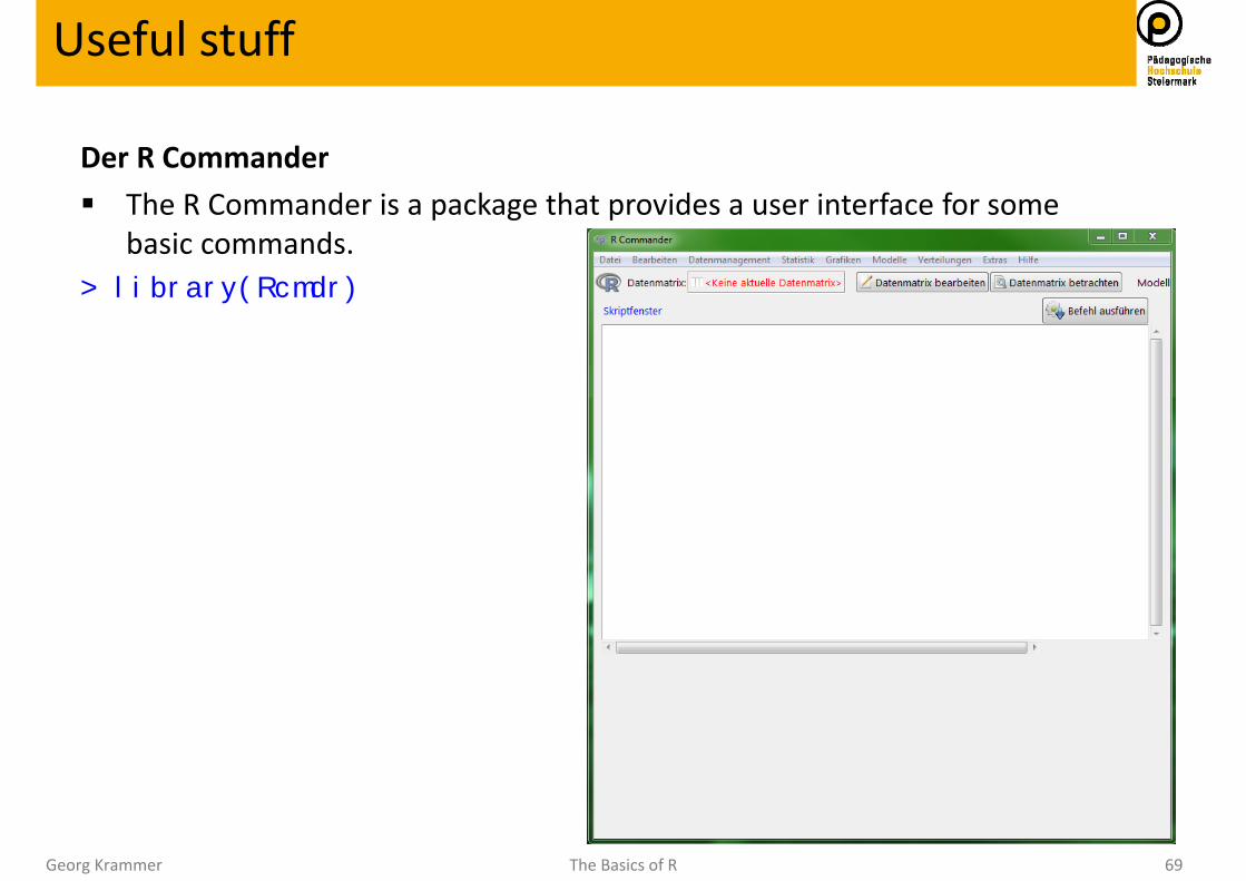
Der R Commander The R Commander is a package that provides a user interface for some
basic commands. > library(Rcmdr)
Useful stuff
Georg Krammer The Basics of R 70
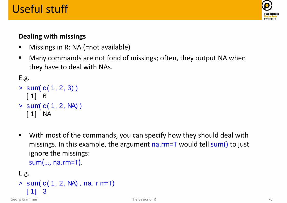
Dealing with missings Missings in R: NA (=not available) Many commands are not fond of missings; often, they output NA when
they have to deal with NAs.E.g.> sum(c(1,2,3)) [1] 6
> sum(c(1,2,NA)) [1] NA
With most of the commands, you can specify how they should deal withmissings. In this example, the argument na.rm=T would tell sum() to just ignore the missings:sum(…, na.rm=T).
E.g.> sum(c(1,2,NA),na.rm=T) [1] 3
Useful stuff
Georg Krammer The Basics of R 71
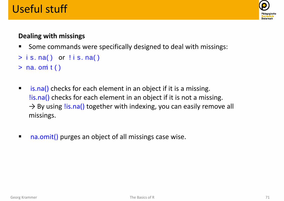
Dealing with missings Some commands were specifically designed to deal with missings:> is.na() or !is.na()
> na.omit()
is.na() checks for each element in an object if it is a missing. !is.na() checks for each element in an object if it is not a missing. → By using !is.na() together with indexing, you can easily remove all missings.
na.omit() purges an object of all missings case wise.
Useful stuff

Georg Krammer The Basics of R 72
And now we are at the end…
Georg Krammer The Basics of R 73
1) What did you like about the workshop?
2) What did you not like as much?
3) What should have been different?
4) Any further remarks?
Feedback