the basic principles of metric indexing · the basic principles of metric indexing magnus lie...

The Basic Principles of Metric Indexing

Magnus Lie Hetland

Norwegian University of Science and Technology

Summary. This chapter describes several methods of similarity search, based onmetric indexing, in terms of their common, underlying principles. Several approachesto creating lower bounds using the metric axioms are discussed, such as pivoting andcompact partitioning with metric ball regions and generalized hyperplanes. Finally,pointers are given for further exploration of the subject, including non-metric, ap-proximate, and parallel methods.

Introduction

This chapter is a tutorial – a brief introduction to the field of metric indexing,which is a way of optimizing certain kinds of similarity retrieval. While thereare several excellent publications that cover this area, this chapter takes aslightly different approach in several respects.1 Primarily, it focuses on givinga concise explanation of underlying principles rather than a comprehensivesurvey of specific methods (which means that some methods are explained inways that differ significantly from the original publications). Also, the maineffort has been put into explaining these principles clearly, rather than goingin depth theoretically or covering the full breadth of the field.

The first two sections of this chapter provide an overview of the main goalsand principles of similarity retrieval in general. Section 3 discusses the specificsof metric spaces, and the following sections deal with three approaches tometric indexing: pivoting, ball partitioning, and generalized hyperplane par-titioning. Section 7 summarizes some methods and issues that aren not dealtwith in detail elsewhere, and finally the appendices give some mathematicaldetails, as well as a listing of all the specific indexing methods discussed inthe chapter. To enhance the flow of the text, many technical details have beenrelegated to end notes, which can be found on pp. 22–29.

2 Magnus Lie Hetland

1 The Goals of Distance Indexing

Similarity search is a mode of information retrieval where the query is a sam-ple object, and the desired result is a set of objects deemed to be similar –in some sense – to the query. The similarity is usually formalized (inversely)as a so-called distance function,∗ and indexing is any form of preprocessing ofthe data set designed to facilitate efficient retrieval.2 The applications rangefrom entertainment and multimedia (such as image or music search) to sci-ence and medicine (such as data mining or matching biological sequences),or anything else that requires efficient query-by-example, but where tradi-tional (coordinate-based) spatial access methods cannot be used. Beyond di-rect search, similarity retrieval can be used as an internal component in a widespectrum of systems, such as nearest neighbor classification (with large samplesets), compressed video streaming (to reuse image patches) and multiobjectiveoptimization (to avoid near-duplication of solutions).3

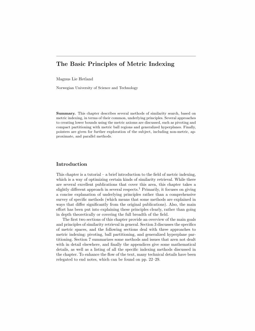
Under the distance function formalism, several query types may be for-mulated. In the following I focus on one of the basic kinds, so-called rangequeries, where all objects that fall within a given distance of the sample arereturned. In other words, for a distance function d, a query object q, and asearch radius r, objects x for which d(q, x) ≤ r are returned (see Fig. 1 on thefacing page). While alternatives are discussed in the literature (most notablyreturning the nearest object, or the k nearest objects) it can be argued thatrange queries are fundamental, and virtually all published metric indexingmethods support them. (For more information about other query types, seeSect. 7.)

Index structures (such as the inverted files traditionally used in text search)are structures built over the given data set in order to speed up queries. Thetime cost involved in building the index is amortized over the series of queries,and is usually ignored when considering search cost. The main goal, then, ofan index method is to enable efficient search, either asymptotically or simplyin real wall-clock time. However, in any specialized form of search there maybe a few wrinkles to the story; for example, in examining an index structuretheoretically, some basic operations of the search algorithm may completelydominate others, but it may not be entirely clear which ones are the morecostly, and there may be different constraints (such as memory use) or requiredpieces of functionality (such as being able to accomodate new objects) that

∗A distance function (or simply a distance) d is a non-negative, real-valued, binaryfunction that is reflexive (d(x, x) = 0) and symmetric (d(x, y) = d(y, x)). The func-tion is defined over some universe of possible objects, U (that is, it has the signatured : U2 → R+

0 ). Both here and later on in the chapter, constraints are implicitly quan-tified over U; for example, symmetry implies that d(x, y) = d(y, x) for all objects x, yin U. When discussing queries, it is assumed that query objects may be arbitrarilychosen from U, while the returned objects are taken from some finite subset D ⊆ U(the data set).

The Basic Principles of Metric Indexing 3

qr

Fig. 1. Visualization of a range query in two-dimensional Euclidean space. Thesmall circles are objects in the data set, while the filled dots are returned as a resultof the query with sample object q and search radius r

influence what the criteria of optimization are. The three most importantmeasures of quality used in the literature are:

• The number of distance computation needed during a query;• The number of I/O operations (disk accesses) needed; and• The CPU time used beyond distance computations or I/O operations.

Of these three, the first is of primary importance, mainly because it isgenerally assumed that the distance computations (which may involve com-paring highly complex objects, such as video clips) are expensive enough tocompletely dominate the running time. Beyond this, some (mostly more re-cent) methods provide mechanisms for going beyond main memory withoutincurring an inordinate number of disk accesses, and many methods also in-volve “tricks” for cutting down on the CPU time. It is quite clear, though,that an underlying assumption for most of the field is that minimizing thenumber of distance computation is the main goal.4

2 Domination, Signatures, and Aggregation

Without even considering the specifics of metric spaces, it is possible to out-line some mechanisms that can be of use when implementing distance indices.This section discusses some fundamental principles, which may then be im-plemented, so to speak, using metric properties (dealt with in the followingsection), as shown in sections 4 through 6.

The most basic algorithm for similarity retrieval (or any form of search)is the linear scan: Traverse the entire data set, examining each object foreligibility.5 In order to improve upon the linear scan, we must somehow inferthat an object x can be included in, or excluded from, the search result withoutcalculating d(q, x). The way to go is to find a cheap way of approximating thedistance. In order to avoid wrongfully including or excluding objects, we needan approximation with certain properties.6 In particular, the approximateddistance must either overestimate or underestimate the actual distance, and


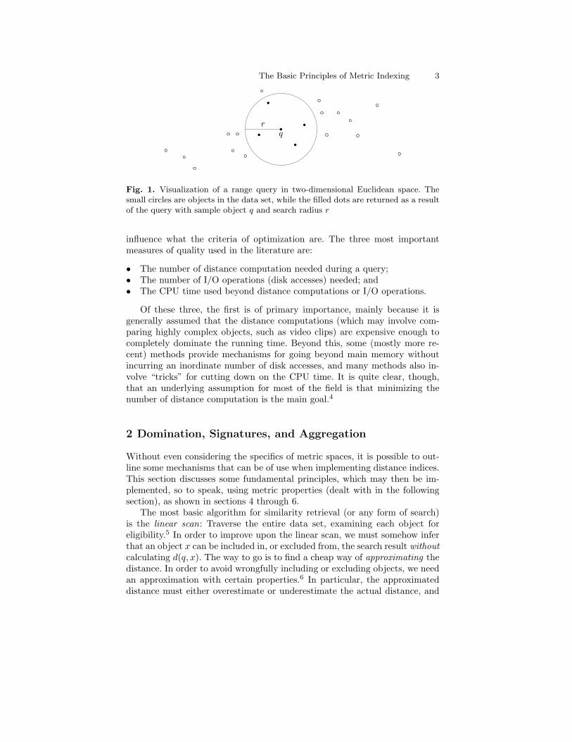
must do so consistently. If the distance function d consistently yields highervalues than another distance function d (over the same set of objects), we saythat d dominates d.

d(q, y)maybe

d(q, y)no

d(q, x)yes

d(q, x)maybe

q x y

Fig. 2. Filtering through distance estimates. The vertical hatched line representsthe range of the query; if an overestimated distance (d) falls within the range, theobject is included, and if an underestimated distance (d) falls beyond it, the objectis discarded. Otherwise, the true distance must be computed

Let d be a distance that dominates the actual distance d (i.e., it forms anupper bound to d), and let d dominate another distance d (a lower bound).These estimates may then be used to partition the data set into three cate-gories: no, yes, and maybe. If d(q, o) > r, the object o may be safely excluded(because no objects may, under d, be “closer than they appear”). Conversely,if d(q, o) ≤ r, the object o may be safely included. The actual distance d(q, o)must then be calculated for any objects that do not satisfy either criterion.See Fig. 2 above and Fig. 3 on the facing page for illustrations of this princi-ple. The more closely d and d approximate d, the smaller the maybe set willbe; however, there will normally be a tradeoff between approximation qualityand cost of computation. One example of this kind of tradeoff is when thereare several sources of knowledge available, and thus several upper and lowerbounds; these may easily be combined, by letting d be the minimum of theupper bounds and d, the maximum of the lower bounds.

Note that under the (quite reasonable) assumption that most of the dataset will not be returned in most queries, the notion of lower bounds andautomatic exclusion is more important than that of upper bounds and auto-matic inclusion. Thus, a major theme in the quest for better distance indexingstructures is the search for ever more accurate, yet still cheap, lower-boundingestimates.

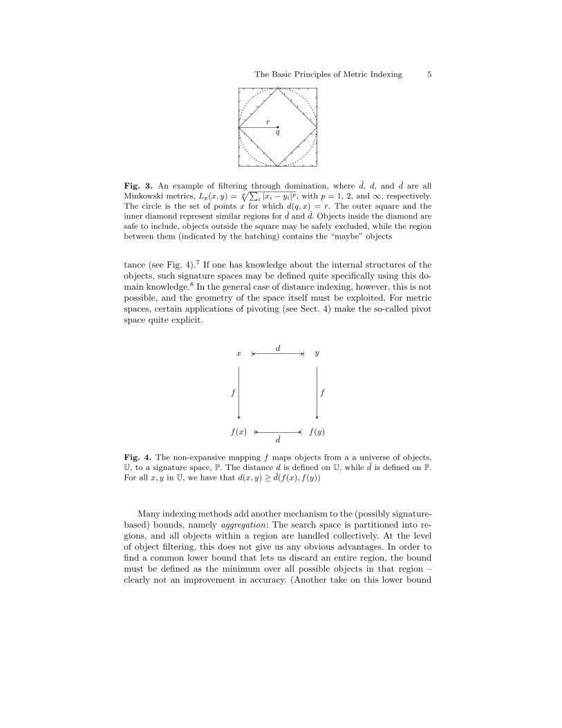
One way of viewing such lower bounds is in terms of so-called non-expansive mappings: All objects are mapped to new objects, or signatures,and the signature distance becomes an underestimate for the original dis-


qr

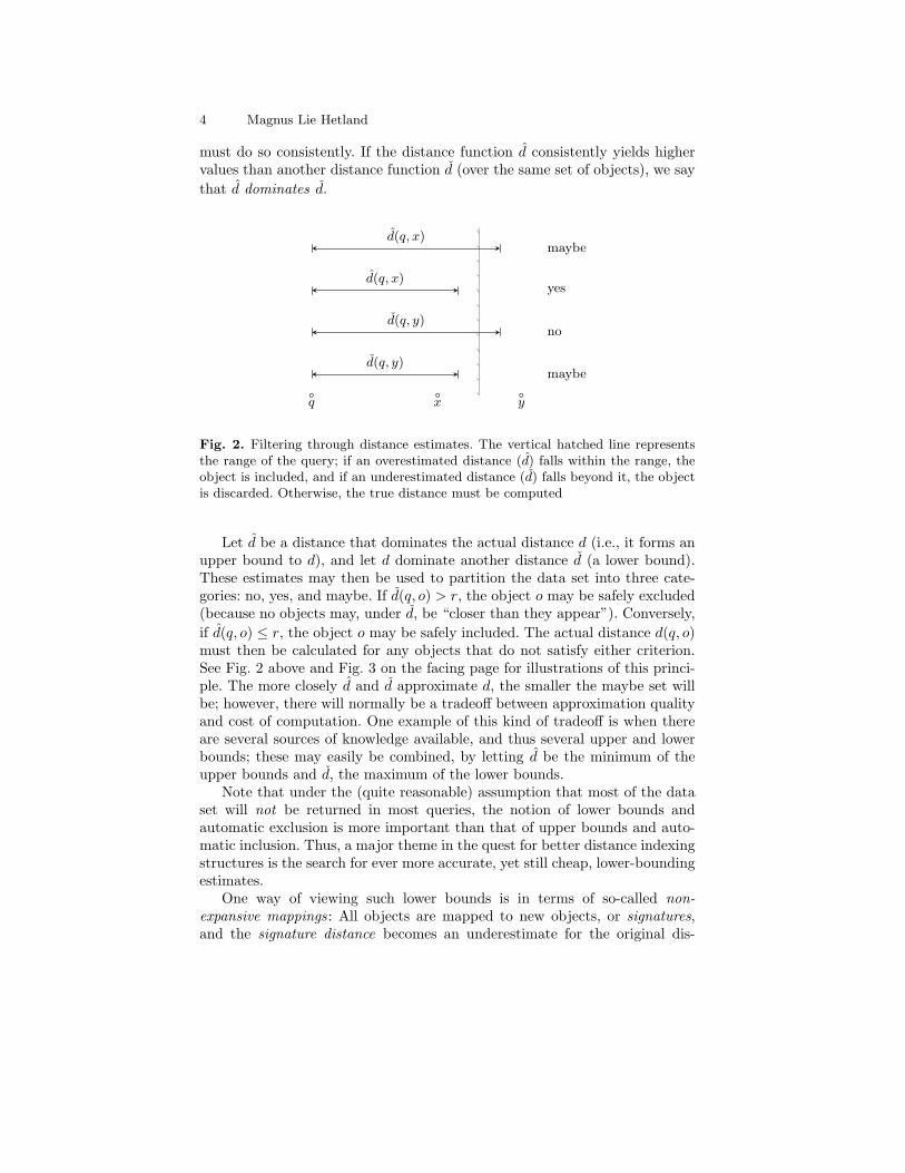
Fig. 3. An example of filtering through domination, where d, d, and d are allMinkowski metrics, Lp(x, y) = p

pPi |xi − yi|p, with p = 1, 2, and ∞, respectively.

The circle is the set of points x for which d(q, x) = r. The outer square and theinner diamond represent similar regions for d and d. Objects inside the diamond aresafe to include, objects outside the square may be safely excluded, while the regionbetween them (indicated by the hatching) contains the “maybe” objects

tance (see Fig. 4).7 If one has knowledge about the internal structures of theobjects, such signature spaces may be defined quite specifically using this do-main knowledge.8 In the general case of distance indexing, however, this is notpossible, and the geometry of the space itself must be exploited. For metricspaces, certain applications of pivoting (see Sect. 4) make the so-called pivotspace quite explicit.

x y

f(x) f(y)

f f

d

d

Fig. 4. The non-expansive mapping f maps objects from a a universe of objects,U, to a signature space, P. The distance d is defined on U, while d is defined on P.For all x, y in U, we have that d(x, y) ≥ d(f(x), f(y))

Many indexing methods add another mechanism to the (possibly signature-based) bounds, namely aggregation: The search space is partitioned into re-gions, and all objects within a region are handled collectively. At the levelof object filtering, this does not give us any obvious advantages. In order tofind a common lower bound that lets us discard an entire region, the boundmust be defined as the minimum over all possible objects in that region –clearly not an improvement in accuracy. (Another take on this lower bound


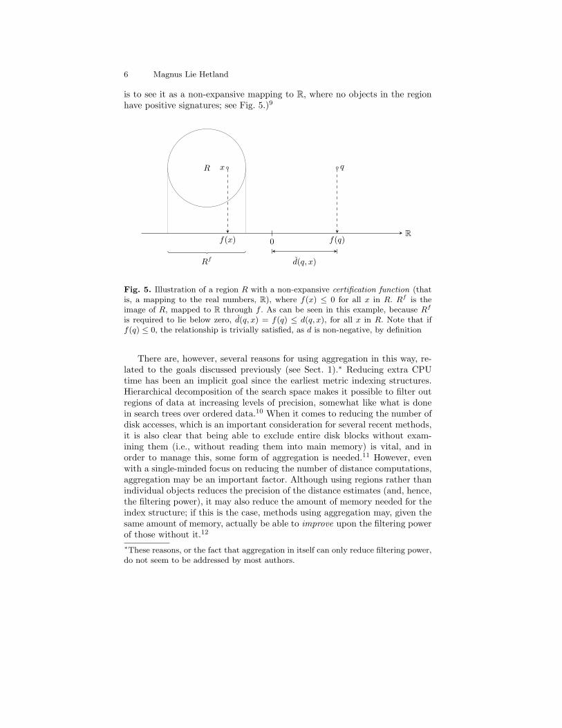
is to see it as a non-expansive mapping to R, where no objects in the regionhave positive signatures; see Fig. 5.)9

R qx

f(x) f(q)R

0

d(q, x)Rf

Fig. 5. Illustration of a region R with a non-expansive certification function (thatis, a mapping to the real numbers, R), where f(x) ≤ 0 for all x in R. Rf is theimage of R, mapped to R through f . As can be seen in this example, because Rf

is required to lie below zero, d(q, x) = f(q) ≤ d(q, x), for all x in R. Note that iff(q) ≤ 0, the relationship is trivially satisfied, as d is non-negative, by definition

There are, however, several reasons for using aggregation in this way, re-lated to the goals discussed previously (see Sect. 1).∗ Reducing extra CPUtime has been an implicit goal since the earliest metric indexing structures.Hierarchical decomposition of the search space makes it possible to filter outregions of data at increasing levels of precision, somewhat like what is donein search trees over ordered data.10 When it comes to reducing the number ofdisk accesses, which is an important consideration for several recent methods,it is also clear that being able to exclude entire disk blocks without exam-ining them (i.e., without reading them into main memory) is vital, and inorder to manage this, some form of aggregation is needed.11 However, evenwith a single-minded focus on reducing the number of distance computations,aggregation may be an important factor. Although using regions rather thanindividual objects reduces the precision of the distance estimates (and, hence,the filtering power), it may also reduce the amount of memory needed for theindex structure; if this is the case, methods using aggregation may, given thesame amount of memory, actually be able to improve upon the filtering powerof those without it.12

∗These reasons, or the fact that aggregation in itself can only reduce filtering power,do not seem to be addressed by most authors.


3 The Geometry of Metric Spaces

In order to qualify as a distance function, a function must normally be sym-metric and reflexive. If d is a distance defined on the universe U, the pair(U, d) is called a distance space. A metric space is a distance space wherenon-identical objects are separated by positive distances and where there areno “short-cuts”: The distance from x to z cannot be improved by going viaanother point (object) y.∗ The distance function of a metric space is called(naturally enough) a metric. One important property of metric spaces is thatsubsets (or subspaces) will also be metric, so if a metric is defined over a givendata type, a finite data set (and relevant queries) of that data type will forma (finite) metric space, subject to the same constraints.

Metric spaces are a generalization of Euclidean space, keeping some of itswell-known geometric properties. These properties allow us to derive certainfacts (and from them, upper and lower bounds) without knowing the exactform of the distance in question.13

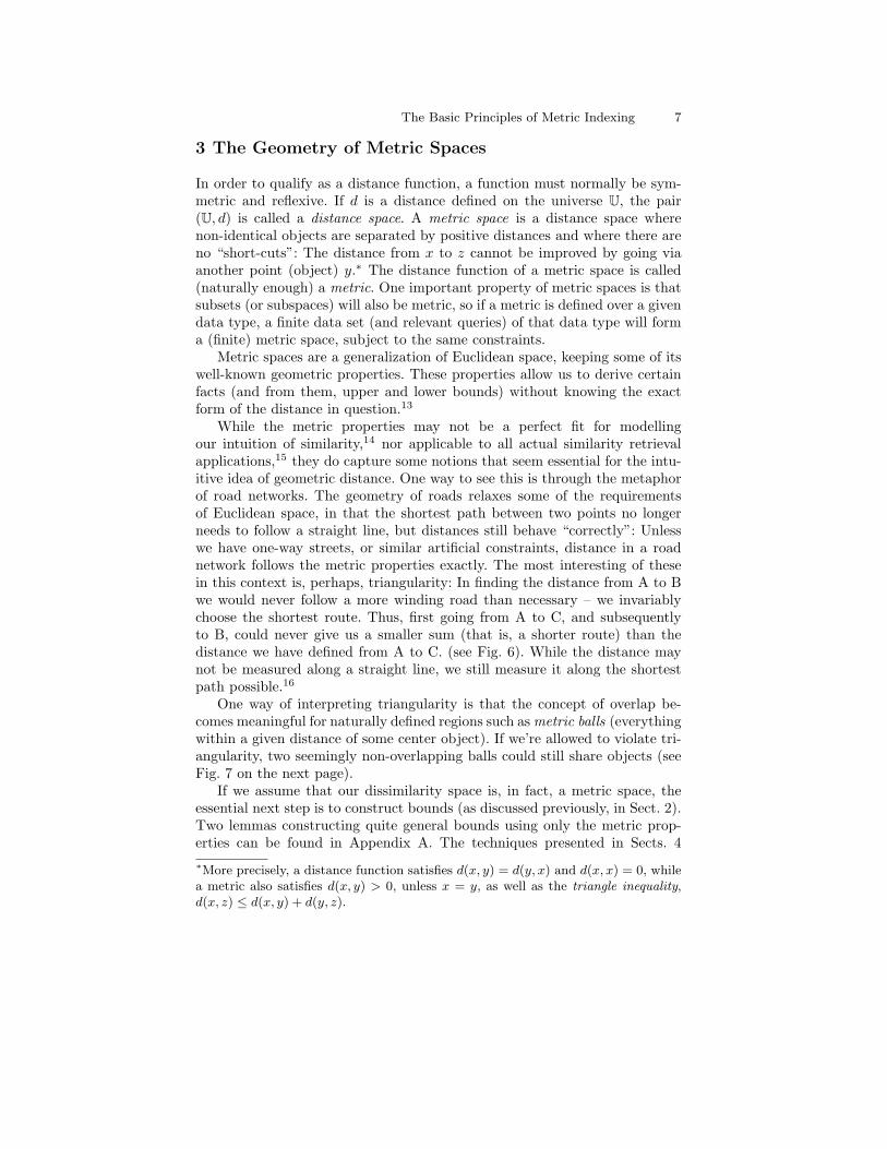
While the metric properties may not be a perfect fit for modellingour intuition of similarity,14 nor applicable to all actual similarity retrievalapplications,15 they do capture some notions that seem essential for the intu-itive idea of geometric distance. One way to see this is through the metaphorof road networks. The geometry of roads relaxes some of the requirementsof Euclidean space, in that the shortest path between two points no longerneeds to follow a straight line, but distances still behave “correctly”: Unlesswe have one-way streets, or similar artificial constraints, distance in a roadnetwork follows the metric properties exactly. The most interesting of thesein this context is, perhaps, triangularity: In finding the distance from A to Bwe would never follow a more winding road than necessary – we invariablychoose the shortest route. Thus, first going from A to C, and subsequentlyto B, could never give us a smaller sum (that is, a shorter route) than thedistance we have defined from A to C. (see Fig. 6). While the distance maynot be measured along a straight line, we still measure it along the shortestpath possible.16

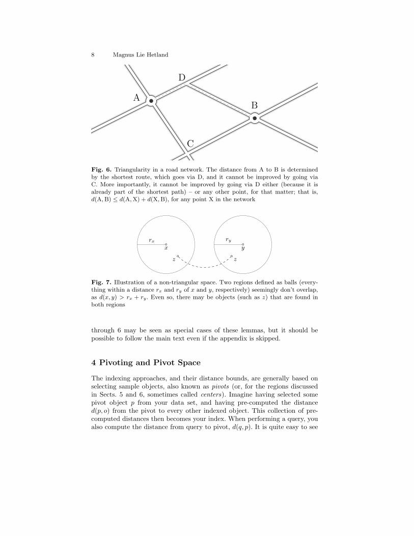
One way of interpreting triangularity is that the concept of overlap be-comes meaningful for naturally defined regions such as metric balls (everythingwithin a given distance of some center object). If we’re allowed to violate tri-angularity, two seemingly non-overlapping balls could still share objects (seeFig. 7 on the next page).

If we assume that our dissimilarity space is, in fact, a metric space, theessential next step is to construct bounds (as discussed previously, in Sect. 2).Two lemmas constructing quite general bounds using only the metric prop-erties can be found in Appendix A. The techniques presented in Sects. 4∗More precisely, a distance function satisfies d(x, y) = d(y, x) and d(x, x) = 0, whilea metric also satisfies d(x, y) > 0, unless x = y, as well as the triangle inequality,d(x, z) ≤ d(x, y) + d(y, z).


AB

C

D

Fig. 6. Triangularity in a road network. The distance from A to B is determinedby the shortest route, which goes via D, and it cannot be improved by going viaC. More importantly, it cannot be improved by going via D either (because it isalready part of the shortest path) – or any other point, for that matter; that is,d(A, B) ≤ d(A, X) + d(X, B), for any point X in the network

x

rx

y

ry

z z

Fig. 7. Illustration of a non-triangular space. Two regions defined as balls (every-thing within a distance rx and ry of x and y, respectively) seemingly don’t overlap,as d(x, y) > rx + ry. Even so, there may be objects (such as z) that are found inboth regions

through 6 may be seen as special cases of these lemmas, but it should bepossible to follow the main text even if the appendix is skipped.

4 Pivoting and Pivot Space

The indexing approaches, and their distance bounds, are generally based onselecting sample objects, also known as pivots (or, for the regions discussedin Sects. 5 and 6, sometimes called centers). Imagine having selected somepivot object p from your data set, and having pre-computed the distanced(p, o) from the pivot to every other indexed object. This collection of pre-computed distances then becomes your index. When performing a query, youalso compute the distance from query to pivot, d(q, p). It is quite easy to see


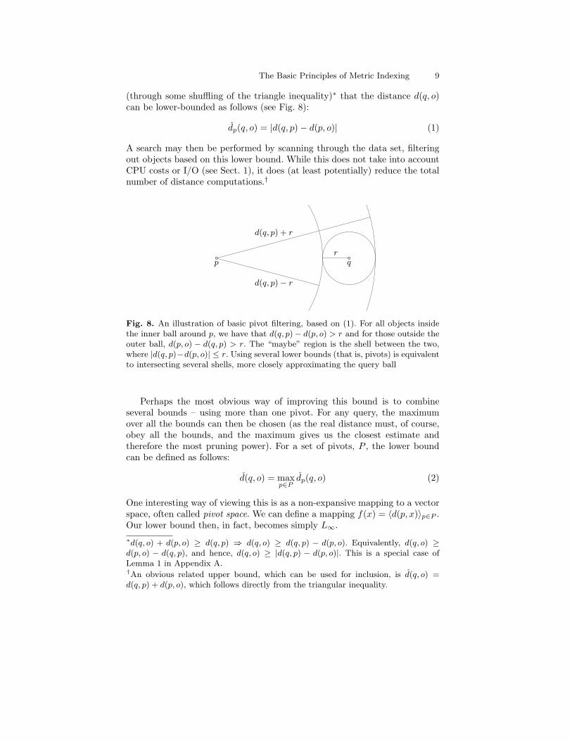
(through some shuffling of the triangle inequality)∗ that the distance d(q, o)can be lower-bounded as follows (see Fig. 8):

dp(q, o) = |d(q, p)− d(p, o)| (1)

A search may then be performed by scanning through the data set, filteringout objects based on this lower bound. While this does not take into accountCPU costs or I/O (see Sect. 1), it does (at least potentially) reduce the totalnumber of distance computations.†

p qr

d(q, p)− r

d(q, p) + r

Fig. 8. An illustration of basic pivot filtering, based on (1). For all objects insidethe inner ball around p, we have that d(q, p)− d(p, o) > r and for those outside theouter ball, d(p, o) − d(q, p) > r. The “maybe” region is the shell between the two,where |d(q, p)−d(p, o)| ≤ r. Using several lower bounds (that is, pivots) is equivalentto intersecting several shells, more closely approximating the query ball

Perhaps the most obvious way of improving this bound is to combineseveral bounds – using more than one pivot. For any query, the maximumover all the bounds can then be chosen (as the real distance must, of course,obey all the bounds, and the maximum gives us the closest estimate andtherefore the most pruning power). For a set of pivots, P , the lower boundcan be defined as follows:

d(q, o) = maxp∈P

dp(q, o) (2)

One interesting way of viewing this is as a non-expansive mapping to a vectorspace, often called pivot space. We can define a mapping f(x) = 〈d(p, x)〉p∈P .Our lower bound then, in fact, becomes simply L∞.∗d(q, o) + d(p, o) ≥ d(q, p) ⇒ d(q, o) ≥ d(q, p) − d(p, o). Equivalently, d(q, o) ≥d(p, o) − d(q, p), and hence, d(q, o) ≥ |d(q, p) − d(p, o)|. This is a special case ofLemma 1 in Appendix A.†An obvious related upper bound, which can be used for inclusion, is d(q, o) =d(q, p) + d(p, o), which follows directly from the triangular inequality.


This, in fact, is the gist of one of the basic metric indexing methods, calledLAESA.17 In LAESA, a set of m pivots is chosen from the data set of sizen, and an n × m matrix is filled with the object-to-pivot distances in a pre-processing step. Searching becomes a linear scan through the matrix, filteringout rows based on the lower bound (2). As the focus is entirely on reducingthe number of comparisons, the linear scan is merely seen as acceptable ex-tra CPU cycles. Some CPU time can be saved by storing columns separately,sorted by distance from its pivot. In each column, the set of viable objectswill be found in a contiguous interval, and this interval can be found by bi-section. One version of the structure even maintains pointers from cells inone column to the next, between those belonging to the same data object,permitting more efficient intersection of the candidate sets.18 The basic ideaof LAESA was rediscovered by Filho et al. (who call it the Omni method),who also index the pivot space using B-trees and R-trees, to reduce CPU timeand I/O.19

The choice of pivots can have quite an effect on the performance of thisbasic pivoting scheme. The simplest approach – simply selecting at random –does work, and several heuristics (such as choosing pivots that are far apartor that have similar distances to each other∗) have been proposed to improvethe filtering power. One approach, in particular, is to heuristically maximizethe lower bound directly. Pivots are added to the pivot set one at a time. Foreach iteration, the choice stands between a set of randomly sampled candidatepivots. In order to evaluate these, a set of pairs of objects is sampled randomlyfrom the data, and the average pivot distance (using the tentative pivot set,including the new candidate in question) is computed. The pivot that gets thehighest average is chosen, and the next iteration begins. 20

The LAESA method is, in fact, based on an older method, called AESA.21

In AESA, there is no separate pivot set; instead, any data object may beused as a pivot, and the set of pivots used depends on the query object.In order to achieve this flexibility (and the resulting unsurpassed pruningpower) one needs to store the distances between all objects in the data setin an n × n matrix (or, rather, half of that, because of symmetry). In thefirst iteration, a pivot is chosen arbitrarily, and the data set is filtered. (Aswe now have the actual distance to the pivot, it can be either included in orexcluded from the final result set.) In subsequent iterations, a pivot is chosenamong the remaining, unfiltered objects. This object should – in order tomaximize pruning power – be as close as possible to the query. This distanceis approximated with the pivot distance (2), using the pivot set built so far.22

In addition to these main algorithms based on pivoting, and their varia-tions, the basic principles are used as components in more complex, hybridstructures.23

∗The latter is the approach used by the Omni method.


5 Metric Balls and Shells

The pivoting scheme can give quite accurate lower bounds, given enough piv-ots. However, that number can be high – in many cases leading to unre-alistically high space requirements.24 One possible tradeoff is to reduce thenumber of pivots below the optimal. As noted in Sect. 2, another possibility isto reduce the information available about each object, through aggregation:Instead of storing the exact distance from an object to a pivot, the object ismerely placed in a region, somehow defined in terms of some of the pivots.This also implies that the relationship between some objects and some pivotscan be left completely undefined.

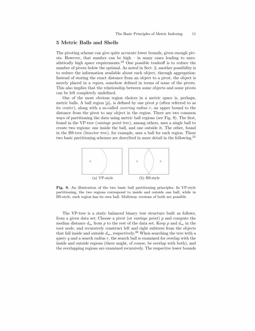
One of the most obvious region choices in a metric space is, perhaps,metric balls. A ball region [p]r is defined by one pivot p (often referred to asits center), along with a so-called covering radius r, an upper bound to thedistance from the pivot to any object in the region. There are two commonways of partitioning the data using metric ball regions (see Fig. 9). The first,found in the VP-tree (vantage point tree), among others, uses a single ball tocreate two regions: one inside the ball, and one outside it. The other, foundin the BS-tree (bisector tree), for example, uses a ball for each region. Thesetwo basic partitioning schemes are described in more detail in the following.25

(a) VP-style (b) BS-style

Fig. 9. An illustration of the two basic ball partitioning principles. In VP-stylepartitioning, the two regions correspond to inside and outside one ball, while inBS-style, each region has its own ball. Multiway versions of both are possible

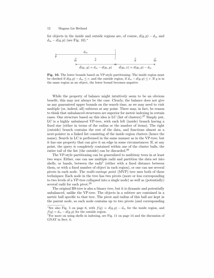
The VP-tree is a static balanced binary tree structure built as follows,from a given data set: Choose a pivot (or vantage point) p and compute themedian distance dm from p to the rest of the data set. Keep p and dm in theroot node, and recursively construct left and right subtrees from the objectsthat fall inside and outside dm, respectively.26 When searching the tree with aquery q and a search radius r, the search ball is examined for overlap with theinside and outside regions (there might, of course, be overlap with both), andthe overlapping regions are examined recursively. The respective lower bounds


for objects in the inside and outside regions are, of course, d(q, p) − dm anddm − d(q, p) (see Fig. 10).∗

p

dm

q1 q2x y

d(q1, y) = dm − d(q1, p) d(q2, x) = d(q2, p)− dm

Fig. 10. The lower bounds based on VP-style partitioning: The inside region mustbe checked if d(q, p)− dm ≤ r, and the outside region, if dm − d(q, p) ≤ r. If q is inthe same region as an object, the lower bound becomes negative

While the property of balance might intuitively seem to be an obviousbenefit, this may not always be the case. Clearly, the balance does not giveus any guaranteed upper bounds on the search time, as we may need to visitmultiple (or, indeed, all) subtrees at any point. There may, in fact, be reasonto think that unbalanced structures are superior for metric indexing in certaincases. One structure based on this idea is LC (list of clusters).27 Simply put,LC is a highly unbalanced VP-tree, with each left (inside) branch having afixed size (either in terms of the radius or the number of items). The right(outside) branch contains the rest of the data, and functions almost as anext-pointer in a linked list consisting of the inside region clusters (hence thename). Search in LC is performed in the same manner as in the VP-tree, butit has one property that can give it an edge in some circumstances: If, at anypoint, the query is completely contained within one of the cluster balls, theentire tail of the list (the outside) can be discarded.28

The VP-style partitioning can be generalized to multiway trees in at leasttwo ways: Either, one can use multiple radii and partition the data set intoshells, or bands, between the radii† (either with a fixed distance betweenthem, or with a fixed number of object in each region), or one can use severalpivots in each node. The multi-vantage point (MVP) tree uses both of thesetechniques: Each node in the tree has two pivots (more or less correspondingto two levels of a VP-tree collapsed into a single node) as well as (potentially)several radii for each pivot.29

The original BS-tree is also a binary tree, but it is dynamic and potentiallyunbalanced, unlike the VP-tree. The objects in a subtree are contained in ametric ball specific to that tree. The pivot and radius of this ball are kept inthe parent node, so each node contains up to two pivots (and corresponding

∗See also Fig. 5 on page 6, with f(q) = d(q, p) − dm for the inside region, andf(q) = dm − d(q, p) for the outside region.†For more on using shells in indexing, see Fig. 11 on page 14 and the discussion ofGNAT in Sect. 6.


radii). When an object is inserted into a node with zero or one pivots, it isadded as a pivot to that node (with an empty subtree). If a node is alreadyfull, the pivot is inserted into the subtree of the nearest pivot.30

The BS-tree has some closely related descendants31 but one of the mostwell-known structures using BS-style ball partitioning is rarely presented asone of them: The M-tree.32

The structures in the M-tree family are, at their core, multiway BS-trees,with each subtree contained in a metric ball, and new objects inserted intothe closest ball (if inside, the one with the closest pivot; if outside, the onewhose radius will increase the least). While more recents structures based onthe M-tree may have extra features (such as special heuristics for insertionor balancing, or AESA-like pivot filtering in each node) this basic structureis common to them all. The main contribution of the M-tree, however, is notsimply the use of a multiway tree structure; it is the way it is implemented– as a balanced, disk-based tree. Each node is a disk block, and balancing isachieved through algorithms quite similar to those of the B-tree family (orthe spatial index structures of the R-tree family).33 This means that it isdynamic (with support for insertions and deletions) and that it is usable forlarge, disk-based data sets.

The iDistance method is a somewhat related approach. Like in the M-tree, the data set is partitioned into ball regions, and one-dimensional pivotfiltering is used within each region. However, instead of using a custom datastructure, all information about regions and pivot distances is stored in a B+-tree. Each object receives a key that, in effect, consists of two digits: The firstis the number of its region, and the second is its distance to the region pivot.A metric search can then be reduced to a set of one-dimensional searches inthe B+-tree – one for each region that overlaps the query.34

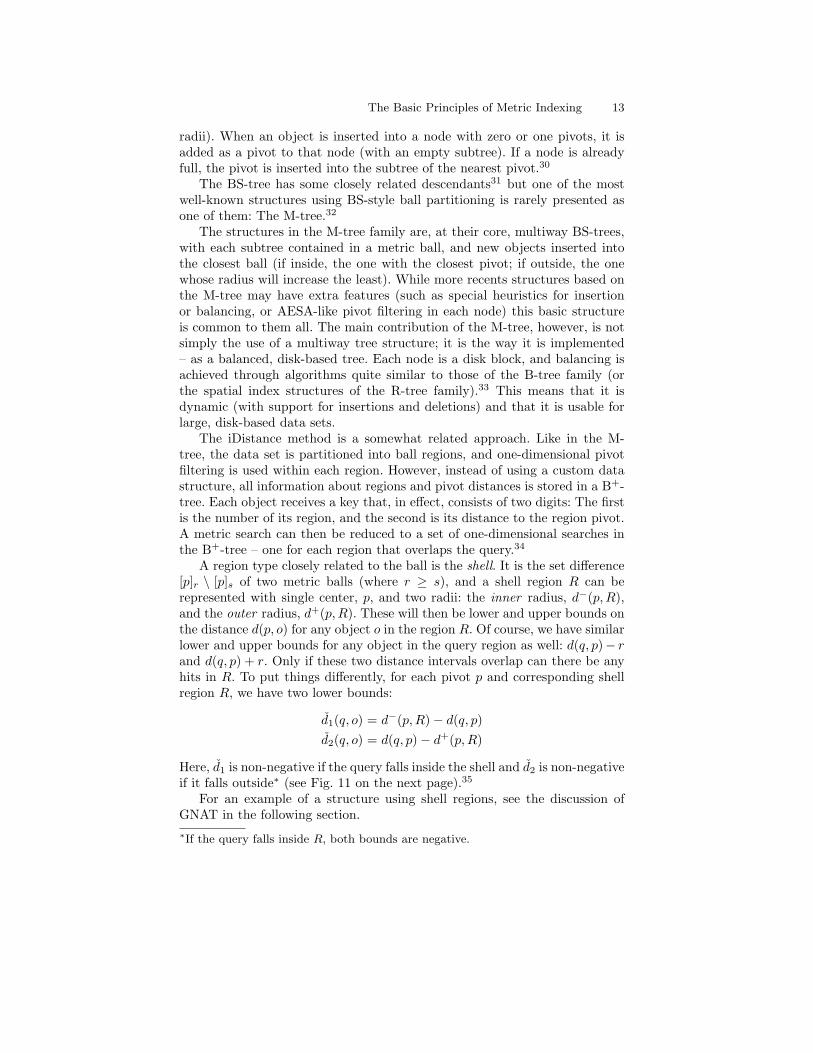
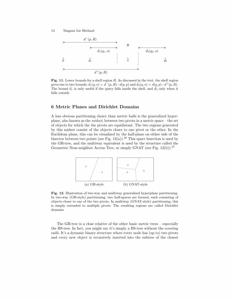
A region type closely related to the ball is the shell. It is the set difference[p]r \ [p]s of two metric balls (where r ≥ s), and a shell region R can berepresented with single center, p, and two radii: the inner radius, d−(p, R),and the outer radius, d+(p, R). These will then be lower and upper bounds onthe distance d(p, o) for any object o in the region R. Of course, we have similarlower and upper bounds for any object in the query region as well: d(q, p)− rand d(q, p) + r. Only if these two distance intervals overlap can there be anyhits in R. To put things differently, for each pivot p and corresponding shellregion R, we have two lower bounds:

d1(q, o) = d−(p, R)− d(q, p)d2(q, o) = d(q, p)− d+(p, R)

Here, d1 is non-negative if the query falls inside the shell and d2 is non-negativeif it falls outside∗ (see Fig. 11 on the next page).35

For an example of a structure using shell regions, see the discussion ofGNAT in the following section.∗If the query falls inside R, both bounds are negative.


p q1 q2

d1(q1, o) d2(q2, o)

d−(p, R)

d+(p, R)

o

R

Fig. 11. Lower bounds for a shell region R. As discussed in the text, the shell regiongives rise to two bounds: d1(q, o) = d−(p, R)−d(q, p) and d2(q, o) = d(q, p)−d+(p, R).The bound d1 is only useful if the query falls inside the shell, and d2 only when itfalls outside

6 Metric Planes and Dirichlet Domains

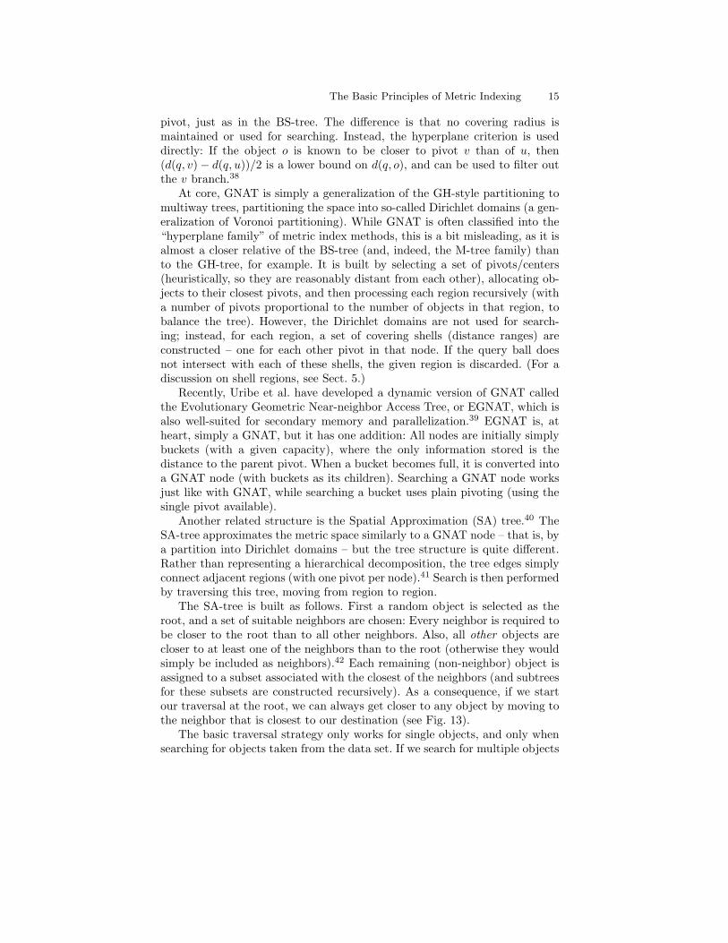
A less obvious partitioning choice than metric balls is the generalized hyper-plane, also known as the midset, between two pivots in a metric space – the setof objects for which the the pivots are equidistant. The two regions generatedby this midset consist of the objects closer to one pivot or the other. In theEuclidean plane, this can be visualized by the half-plane on either side of thebisector between two points (see Fig. 12(a)).36 This space bisection is used bythe GH-tree, and the multiway equivalent is used by the structure called theGeometric Near-neighbor Access Tree, or simply GNAT (see Fig. 12(b)).37

(a) GH-style (b) GNAT-style

Fig. 12. Illustration of two-way and multiway generalized hyperplane partitioning.In two-way (GH-style) partitioning, two half-spaces are formed, each consisting ofobjects closer to one of the two pivots. In multiway (GNAT-style) partitioning, thisis simply extended to multiple pivots. The resulting regions are called Dirichletdomains

The GH-tree is a close relative of the other basic metric trees – especiallythe BS-tree. In fact, you might say it’s simply a BS-tree without the coveringradii. It’s a dynamic binary structure where every node has (up to) two pivotsand every new object is recursively inserted into the subtree of the closest


pivot, just as in the BS-tree. The difference is that no covering radius ismaintained or used for searching. Instead, the hyperplane criterion is useddirectly: If the object o is known to be closer to pivot v than of u, then(d(q, v)− d(q, u))/2 is a lower bound on d(q, o), and can be used to filter outthe v branch.38

At core, GNAT is simply a generalization of the GH-style partitioning tomultiway trees, partitioning the space into so-called Dirichlet domains (a gen-eralization of Voronoi partitioning). While GNAT is often classified into the“hyperplane family” of metric index methods, this is a bit misleading, as it isalmost a closer relative of the BS-tree (and, indeed, the M-tree family) thanto the GH-tree, for example. It is built by selecting a set of pivots/centers(heuristically, so they are reasonably distant from each other), allocating ob-jects to their closest pivots, and then processing each region recursively (witha number of pivots proportional to the number of objects in that region, tobalance the tree). However, the Dirichlet domains are not used for search-ing; instead, for each region, a set of covering shells (distance ranges) areconstructed – one for each other pivot in that node. If the query ball doesnot intersect with each of these shells, the given region is discarded. (For adiscussion on shell regions, see Sect. 5.)

Recently, Uribe et al. have developed a dynamic version of GNAT calledthe Evolutionary Geometric Near-neighbor Access Tree, or EGNAT, which isalso well-suited for secondary memory and parallelization.39 EGNAT is, atheart, simply a GNAT, but it has one addition: All nodes are initially simplybuckets (with a given capacity), where the only information stored is thedistance to the parent pivot. When a bucket becomes full, it is converted intoa GNAT node (with buckets as its children). Searching a GNAT node worksjust like with GNAT, while searching a bucket uses plain pivoting (using thesingle pivot available).

Another related structure is the Spatial Approximation (SA) tree.40 TheSA-tree approximates the metric space similarly to a GNAT node – that is, bya partition into Dirichlet domains – but the tree structure is quite different.Rather than representing a hierarchical decomposition, the tree edges simplyconnect adjacent regions (with one pivot per node).41 Search is then performedby traversing this tree, moving from region to region.

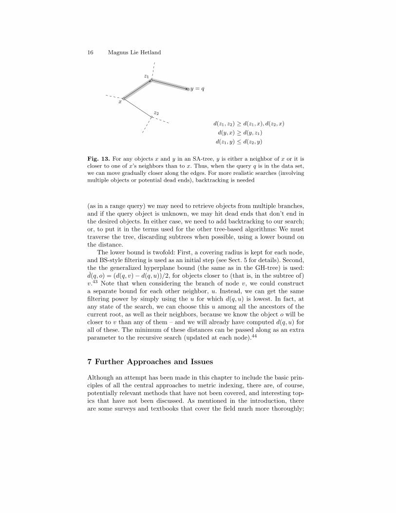
The SA-tree is built as follows. First a random object is selected as theroot, and a set of suitable neighbors are chosen: Every neighbor is required tobe closer to the root than to all other neighbors. Also, all other objects arecloser to at least one of the neighbors than to the root (otherwise they wouldsimply be included as neighbors).42 Each remaining (non-neighbor) object isassigned to a subset associated with the closest of the neighbors (and subtreesfor these subsets are constructed recursively). As a consequence, if we startour traversal at the root, we can always get closer to any object by moving tothe neighbor that is closest to our destination (see Fig. 13).

The basic traversal strategy only works for single objects, and only whensearching for objects taken from the data set. If we search for multiple objects


x

z1

z2

y = q

d(z1, z2) ≥ d(z1, x), d(z2, x)

d(y, x) ≥ d(y, z1)

d(z1, y) ≤ d(z2, y)

Fig. 13. For any objects x and y in an SA-tree, y is either a neighbor of x or it iscloser to one of x’s neighbors than to x. Thus, when the query q is in the data set,we can move gradually closer along the edges. For more realistic searches (involvingmultiple objects or potential dead ends), backtracking is needed

(as in a range query) we may need to retrieve objects from multiple branches,and if the query object is unknown, we may hit dead ends that don’t end inthe desired objects. In either case, we need to add backtracking to our search;or, to put it in the terms used for the other tree-based algorithms: We musttraverse the tree, discarding subtrees when possible, using a lower bound onthe distance.

The lower bound is twofold: First, a covering radius is kept for each node,and BS-style filtering is used as an initial step (see Sect. 5 for details). Second,the the generalized hyperplane bound (the same as in the GH-tree) is used:d(q, o) = (d(q, v)− d(q, u))/2, for objects closer to (that is, in the subtree of)v.43 Note that when considering the branch of node v, we could constructa separate bound for each other neighbor, u. Instead, we can get the samefiltering power by simply using the u for which d(q, u) is lowest. In fact, atany state of the search, we can choose this u among all the ancestors of thecurrent root, as well as their neighbors, because we know the object o will becloser to v than any of them – and we will already have computed d(q, u) forall of these. The minimum of these distances can be passed along as an extraparameter to the recursive search (updated at each node).44

7 Further Approaches and Issues

Although an attempt has been made in this chapter to include the basic prin-ciples of all the central approaches to metric indexing, there are, of course,potentially relevant methods that have not been covered, and interesting top-ics that have not been discussed. As mentioned in the introduction, thereare some surveys and textbooks that cover the field much more thoroughly;


the remainder of this section elaborates on the the scope of the chapter, andpoints to some sources of further information.

Other query types.

The range search is, in many ways, the least complex of the distance basedquery modes. Some other types include the following [see 3].

• Nearest or farthest neighbors: Find the k objects that are nearest to orfurthest from the query object.

• Closest or most distant pair: Find the two object that are closest to ormost distant from each other. Sometimes known as similarity self-join.

• Ranking and inverse ranking: Traverse the objects in (inverse) order ofdistance from the query.

• Combinations, such as finding the (at most) k nearest objects within asearch radius of r.

Of these, the k-nearest-neighbor (kNN) search (possibly combined withrange search) is by far the most common, and perhaps the most intuitivefrom the user and application point of view. Some principles discussed in thischapter – such as domination and non-expansive mappings – do not transferdirectly to the case of kNN search. In order for a transform between distancespaces to preserve the k nearest neighbors, it must preserve the relative dis-tances from the query to these objects; simply underestimating them is notenough to guarantee a correct result. Even so, the techniques behind rangesearch can be used quite effectively to perform kNN searches as well.

Although there are special-purpose kNN mechanisms for some index struc-tures, the general approach is to perform what amounts to a branch-and-bound search: If a given object (or set of objects) cannot improve upon thesolution we have found so far, it is discarded. More specifically, we maintain acandidate set as the index is examined, consisting of the (at most) k nearestneighbors found so far, along with a dynamic query radius that tightly coversthe current candidates.∗

As the search progresses, we want to know if we can find any objects thatwill improve our candidate set; any such objects would have to fall within thecurrent query radius (as they would have to be closer to the query object thanthe furthest current candidate). Thus, we can use existing radius-based searchtechniques, shrinking the radius as new candidates are found. The magnitudeof the covering radius will then be crucial for search efficiency. It can be keptlow for most of the search by heuristically seeking out good candidates earlyon, for example by visiting regions that are close to the query before thosethat are further away [3].

Take one of the simplest index structures, the BS-tree (see p. 11). Fora range query, subtrees are discarded if their covering balls don’t intersect∗Until we have k candidates, the covering radius is infinite.


the query. For a kNN search, we use the candidate ball instead: Only if it isintersected is there any hope of finding a closer neighbor.

Another perspective can be found in the original 1-NN versions of pivotingmethods such as AESA and its relatives (see p. 10). They alternate betweentwo steps:

1. Heuristically choose a promising neighbor and compute the actual distanceto it from the query.

2. Use the pivoting lower bound to eliminate all objects that are furtheraway than the current candidate.

Both the heuristic and the lower bound are based on the set of candidateschosen so far (that is, they are used as pivots). While it might seem like adifferent approach, this too is really just a matter of maintaining a shrinkingquery ball with the current candidates, and the method readily generalizes tokNN for k > 1.

Other indexing approaches.

While the principles of distance described in Sect. 2 hold in general, in thediscussions of particulars in the previous sections, several approaches havedeliberately been left out. Some important ones are:

• Coordinate-based, or spatial, access methods (see the textbook on the sub-ject by Samet [4] for extensive information on multidimensional indexing).This includes methods in the borderland between purely distance-basedmethods and spatial ones, such as the M+- and BM+-trees of Zhou et al.[5, 6].

• Coordinate-based vector space embeddings, such as FastMap [7]. Whilepivot space mapping (as used in LAESA [8] and Omni [1]) is an embeddinginto a vector space (Rk under L∞) it is not based on the initial objectshaving coordinates.

• Approximate methods, such as approximate search with the M-tree [9],MetricMap [10], kNN graphs [see, e.g., 4, pp. 637–641], SASH [11], theproximity preserving order of Chavez et al. [12] or several others [13–15].

• Methods based on stronger assumptions than the metric axioms, such asthe growth-restricted metrics of Karger and Ruhl [16].

• Methods based on weaker assumptions than the metric axioms, such asthe TriGen method of Skopal [17, 18].∗

• Methods exploiting the properties of discrete distances (or discrete metrics,in particular), such as the Burkhart-Keller tree, and The Fixed-Query Treeand its relatives.45

∗Some approximate methods, such as SASH, kNN graphs, and the proximity pre-serving order of Chavez et al. also waive the metric axioms in favor of more heuristicideas of how a distance behaves.


• Methods dealing with query types other than range search,∗ such as thesimilarity self-join (nearest pair queries) of the eD-index [19], the multi-metric or complex searches of M3-tree [20] and others [21–24], searchingwith user-defined metrics, as in the QIC-M-tree [25], or the incrementalsearch of Hjaltason and Samet [26].

• Parallel and distributed methods, using several processors (beyond simpledata partitioning), such as GHT∗ [27], MCAN [28], parallel EGNAT [29]and several other approaches [25, 28, 30–32].

Metric space dimension.

It is well known that spatial access methods deal more effectively with low-dimensional vector spaces than high-dimensional ones (one aspect of the so-called curse of dimensionality).46 Some attempts have been made to generalizethe concept of dimension to metric spaces as well, in order to measure howdifficult a given space would be to index.

One thing that happens when the dimension increases in Euclidean space,for example, is that all distances become increasingly similar, offset somewhatby any clustering in the data. One hypothesis is that it is this convergenceof distances that makes indexing difficult, and this idea is formalized in theintrinsic dimensionality of Chavez et al. [33]. Rather than dealing with coor-dinates, this measure is defined using the distance distribution of a metric (or,in general, distance) space. The intrinsic dimensionality is defined as µ2/2σ2,where µ and σ2 are the mean and variance of distribution, respectively. For aset of uniformly random vectors, this is actually proportional to the dimensionof the vector space. Note that a large spread of distances results in a lowerdimensionality, and vice versa.

An interesting property of distance distributions with a low spread can beseen when considering the cumulative distribution function N(r), the aver-age number of objects returned for a range query with radius r. For r-valuesaround the mean distance, the value of N will increase quite rapidly – the nar-rower the distribution, the more quickly it will increase. Traina Jr. et al. [34],building on the work on fractal dimensions by Belussi and Faloutsos [35], showthat for many synthetic and real-world metric data sets, for suitable rangesof r, the cumulative distribution follows a power-law; that is, N(r) ∈ Θ(rD),for some constant D, which they call the distance exponent.47 They show howto estimate the distance exponent, and demonstrate that it is closely relatedto, among other things, the number of disk accesses needed when performingrange queries using the M-tree.

Another, rather different, hypothesis is that the problem with high dimen-sionality in vector spaces is the abundance of emptiness: As the dimensiongrows, the ratio of data to the sheer volume of space falls exponentially. It∗While kNN is only briefly discussed in this chapter, most of the methods discussedsupport it.


becomes hard to create tight regions around subsets of the data, and re-gion overlaps abound. The ball-overlap factor (BOF) of Skopal [17] tacklesthis problem head-on, and measures the relative frequency of overlap betweensuitably chosen ball regions. BOFk is defined as the relative frequency of over-lap between balls that each cover an object and its k nearest neighbors. Inother words, it predicts the likelihood that two rather arbitrary ball-shapedregions will overlap. This factor can describe both the degree of overlap bydistinct regions in an index structure, and the the probability that a querywill have to investigate irrelevant ball regions (only non-overlapping regionscan be discarded).

Method quality.

In the introduction, the main goals and quality measures used in the develop-ment of metric indexing methods were briefly discussed, but the full pictureis rather complex. The theoretical analysis of these structures can be quitedifficult, so experimental validation becomes essential. There are some theo-retically defined measures such as the fat and bloat factors and prunabilityof Traina Jr. et al. [36, 37], but even such properties are generally establishedempirically for a given structure.48 Moret [38] gives some reasons why asymp-totic analysis alone may not be enough for algorithm studies in general (theworst-case behavior may be restricted to a very small subset of instances andthus not be at all characteristic of instances encountered in practice, and evenin the absence of these problems, deriving tight asymptotic bounds may bevery difficult). Given a sufficiently problematic metric space, a full linear scancan never be avoided, so the non-asymptotic (primarily empirical) analysismay be particularly relevant for metric indexing.

Even beyond the specifics of a given data set (including measures suchas intrinsic dimensionality, fractal dimension, and ball-overlap factor) thereare, of course, the real-world issues that plague all theoretical studies of algo-rithms, such as caching and the memory hierarchy – issues that are not easilyaddressed in terms of basic principles (at least not given the current state ofthe theory of metric index structures) and therefore have been omitted fromthis chapter.

A Bounding Lemmas, with Proofs

The following two lemmas give us some useful bounds for use in metric index-ing. For a more detailed discussions, see, for example, the survey by Hjaltasonand Samet [3] or the textbook by Zezula et al. [39]. Lemmas 1 and 2 areillustrated in figures 14 and 15, respectively.

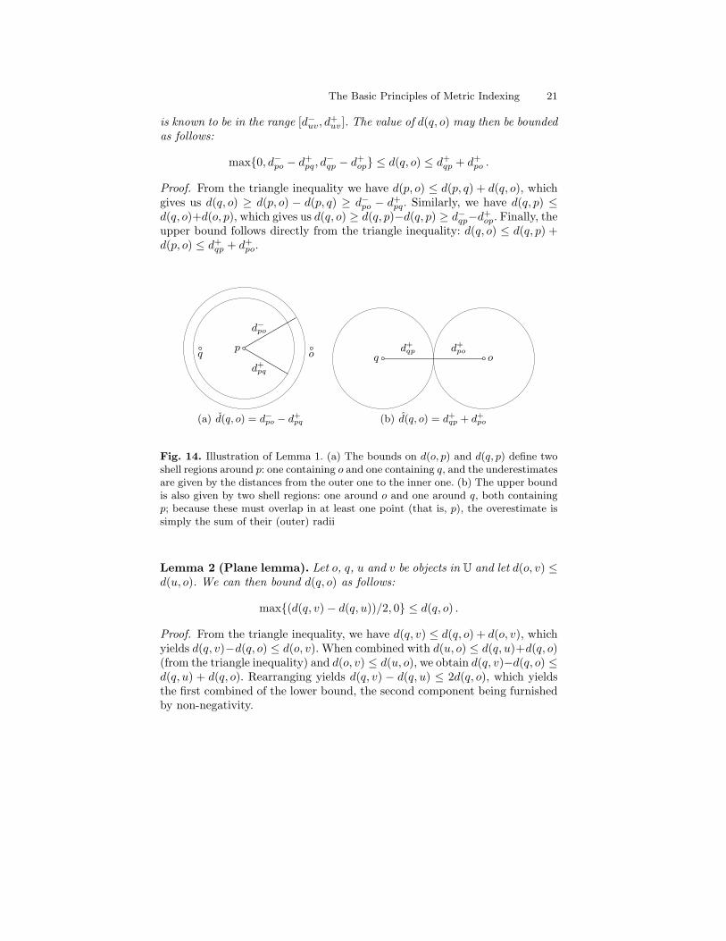
Lemma 1 (Ball lemma). Let o, p and q be objects in U, and let d be ametric over U. For any objects u, v in U, assume that the the value of d(u, v)


is known to be in the range [d−uv, d+uv]. The value of d(q, o) may then be bounded

as follows:

max{0, d−po − d+pq, d

−qp − d+

op} ≤ d(q, o) ≤ d+qp + d+

po .

Proof. From the triangle inequality we have d(p, o) ≤ d(p, q) + d(q, o), whichgives us d(q, o) ≥ d(p, o) − d(p, q) ≥ d−po − d+

pq. Similarly, we have d(q, p) ≤d(q, o)+d(o, p), which gives us d(q, o) ≥ d(q, p)−d(q, p) ≥ d−qp−d+

op. Finally, theupper bound follows directly from the triangle inequality: d(q, o) ≤ d(q, p) +d(p, o) ≤ d+

qp + d+po.

po

d−po

q

d+pq

(a) d(q, o) = d−po − d+pq

qd+

qpo

d+po

(b) d(q, o) = d+qp + d+

po

Fig. 14. Illustration of Lemma 1. (a) The bounds on d(o, p) and d(q, p) define twoshell regions around p: one containing o and one containing q, and the underestimatesare given by the distances from the outer one to the inner one. (b) The upper boundis also given by two shell regions: one around o and one around q, both containingp; because these must overlap in at least one point (that is, p), the overestimate issimply the sum of their (outer) radii

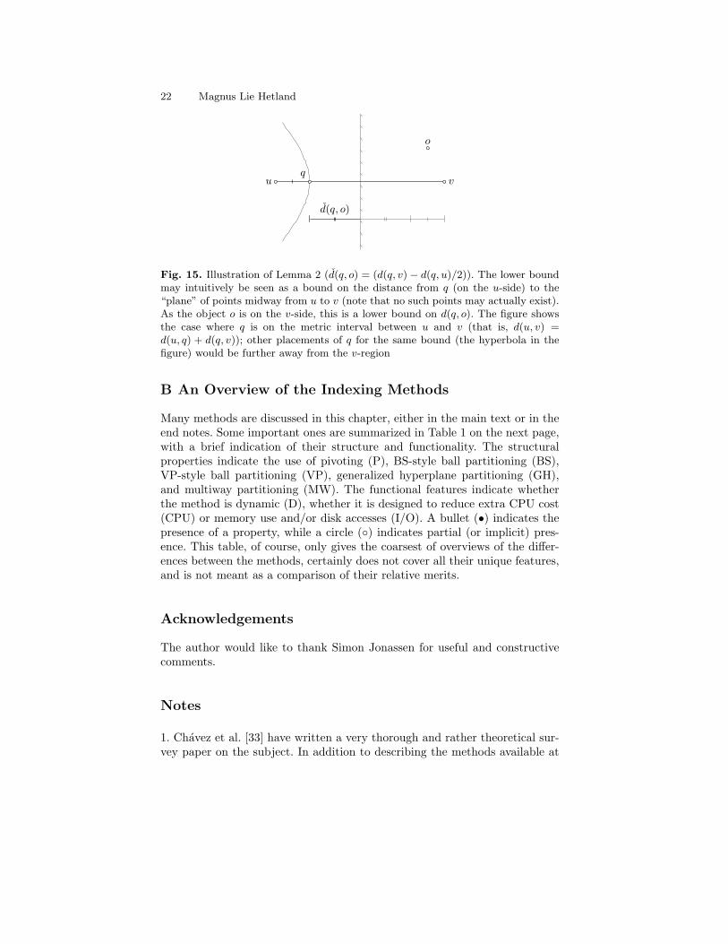
Lemma 2 (Plane lemma). Let o, q, u and v be objects in U and let d(o, v) ≤d(u, o). We can then bound d(q, o) as follows:

max{(d(q, v)− d(q, u))/2, 0} ≤ d(q, o) .

Proof. From the triangle inequality, we have d(q, v) ≤ d(q, o) + d(o, v), whichyields d(q, v)−d(q, o) ≤ d(o, v). When combined with d(u, o) ≤ d(q, u)+d(q, o)(from the triangle inequality) and d(o, v) ≤ d(u, o), we obtain d(q, v)−d(q, o) ≤d(q, u) + d(q, o). Rearranging yields d(q, v) − d(q, u) ≤ 2d(q, o), which yieldsthe first combined of the lower bound, the second component being furnishedby non-negativity.


u v

o

q

d(q, o)

Fig. 15. Illustration of Lemma 2 (d(q, o) = (d(q, v)− d(q, u)/2)). The lower boundmay intuitively be seen as a bound on the distance from q (on the u-side) to the“plane” of points midway from u to v (note that no such points may actually exist).As the object o is on the v-side, this is a lower bound on d(q, o). The figure showsthe case where q is on the metric interval between u and v (that is, d(u, v) =d(u, q) + d(q, v)); other placements of q for the same bound (the hyperbola in thefigure) would be further away from the v-region

B An Overview of the Indexing Methods

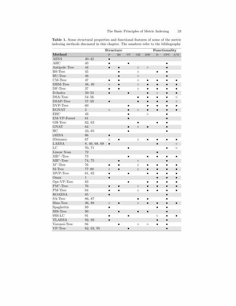
Many methods are discussed in this chapter, either in the main text or in theend notes. Some important ones are summarized in Table 1 on the next page,with a brief indication of their structure and functionality. The structuralproperties indicate the use of pivoting (P), BS-style ball partitioning (BS),VP-style ball partitioning (VP), generalized hyperplane partitioning (GH),and multiway partitioning (MW). The functional features indicate whetherthe method is dynamic (D), whether it is designed to reduce extra CPU cost(CPU) or memory use and/or disk accesses (I/O). A bullet (•) indicates thepresence of a property, while a circle (◦) indicates partial (or implicit) pres-ence. This table, of course, only gives the coarsest of overviews of the differ-ences between the methods, certainly does not cover all their unique features,and is not meant as a comparison of their relative merits.

Acknowledgements

The author would like to thank Simon Jonassen for useful and constructivecomments.

Notes

1. Chavez et al. [33] have written a very thorough and rather theoretical sur-vey paper on the subject. In addition to describing the methods available at


Table 1. Some structural properties and functional features of some of the metricindexing methods discussed in this chapter. The numbers refer to the bibliography

Structure FunctionalityMethod p bs vp gh mw d cpu i/o

AESA 40–42 •AHC 43 • • •Antipole Tree 44 • • ◦ ◦ •BS-Tree 45 • ◦ • •BU-Tree 46 • ◦ •CM-Tree 47 • • ◦ • • • •DBM-Tree 48, 49 ◦ • ◦ • • • •DF-Tree 37 • • ◦ • • • •D-Index 50–53 • • • ◦ • •DSA-Tree 54–56 • • • • ◦DSAP-Tree 57–59 • • • • • ◦DVP-Tree 60 • • • • •EGNAT 2 ◦ • ◦ • • • •EHC 43 • ◦ •EM-VP-Forest 61 • •GH-Tree 62, 63 • • •GNAT 64 • ◦ • •HC 43, 65 • •iAESA 66 •iDistance 67 ◦ • ◦ • • • •LAESA 8, 40, 68, 69 • • ◦LC 70, 71 • • ◦Linear Scan 72 •MB+-Tree 73 • • • • •MB∗-Tree 74, 75 • ◦ •M∗-Tree 76 • • ◦ • • • •M-Tree 77–80 ◦ • ◦ • • • •MVP-Tree 81, 82 • • • • • •Omni 1 • • • •Opt-VP-Tree 83 • • • • •PM∗-Tree 76 • • ◦ • • • •PM-Tree 84 • • ◦ • • • •ROAESA 85 • •SA-Tree 86, 87 • • •Slim-Tree 36, 88 ◦ • ◦ • • • •Spaghettis 89 • • •SSS-Tree 90 • • • •SSS-LC 91 • • ◦ • •TLAESA 92, 93 • • •Voronoi-Tree 94 • ◦ ◦ • •VP-Tree 62, 63, 95 • •


the time, they construct a taxonomy of the methods and derive theoreticalbounds for their complexity. They also introduce the concept of intrinsic di-mensionality (see Sect. 7). The later survey by Hjaltason and Samet [3] takes asomewhat different approach, and uses a different fundamental formalism, butis also quite comprehensive and solid, and complements the paper by Chavezet al. nicely. In recent years, a textbook on the subject by Zezula et al. hasappeared [39], and Sect. 4.5 of Samet’s book on multidimensional and metricdata structures [4] is also devoted to distance based methods. The paper byPestov and Stojmirovic [96] is specifically about a model for similarity search,but in many ways provides a brief survey as well. The encyclopedia entry byChavez and Navarro [97] is another example of a brief introduction. In ad-dition to publications that specifically set out to describe the field, there arealso publications, such as the PhD thesis of Skopal [98], with more specifictopics, that still have substantial sections devoted to the general field of metricindexing.2. Note that the terminology is not entirely consistent across the literature.The use of ‘distance’ here conforms with the usage of Deza and Deza [99].3. Many of the surveys mentioned previously [3, 4, 33, 39, 96–98] discussvarious applications, as do most publications about specific metric indexingmethods. Spatial access methods [see, e.g., 4] can also be used for many query-by-example applications, but they rely on the specific structure of the problem– the fact that all objects are represented as vectors of a space of fixed,low dimensionality. Metric indexing is designed for cases where less is knownabout the space (i.e., where we only know the distances between objects, andthose distances satisfy the metric axioms), and thus have a different, possiblywider, field of applications. Because the metric indexing methods disregard thenumber of dimensions of a vector space and are only hampered by the innatecomplexity of the given distance (or the distribution of objects), they mayalso be better suited to indexing high-dimensional traditional vector spaces(see Sect. 7).4. The field in question is defined by in excess of fifty published methods formetric indexing, stretching back to the 1983 paper of Kalantari and McDonald[45] (with more recent publications including ones by Aronovich and Spiegler[47] and Brisaboa et al. [90], for example), not counting several methods aimedspecifically at discrete distance measures (surveyed along with more generalmethods by Chavez et al. [33]; see also Sect. 7).5. While a linear scan is very straightforward, and seemingly quite inefficient,it may serve as an important “reality check,” particularly for complex indexstructures (especially involving disk access) or high-dimensional data. Theextra work in maintaining and traversing the structures may become so high,in some cases, that it swamps the reduction in distance computations [see,e.g., 72].


6. As discussed in Sect. 7, there are approximate retrieval methods as well,where some such errors are permitted. In these cases, looser notions of distanceapproximation may be acceptable.7. Such mappings are normally defined between metric spaces, and are knownby several names, including metric mappings and 1-Lipschitz mappings.8. One example of this technique is similarity indexing for time series, wheremany signature types have been suggested, normally in the form of fixed-dimensional vectors that may be indexed using spatial access methods. Het-land [100] gives a survey of this application.9. Hjaltason and Samet [3] use hierarchical decompositions of the space into re-gions (represented as tree structures) as their main formalism when discussingindexing methods. In order to discard such a region R from a search, a lowerbound on the point-set distance d(q, R) = infx∈R d(q, x) must be defined;this bound is a characteristic of the region type used. Pestov and Stojmirovic[96] use basically the same formalism, although presented rather differently.Instead of equipping the tree nodes corresponding to regions with lower-bounding distance estimates, they give them certification functions, which arenon-expansive (1-Lipschitz) mappings f : R → R, where f(x) ≤ 0,∀x ∈ R.While not discussed by the authors, it should be clear that these certificationfunctions are equivalent to lower-bounding estimates of the point-set distance(see Fig. 4 on page 5). For a rather different approach, see the survey byChavez et al. [33]. They base their indexing formalism on the hierarchicaldecomposition of the search space into equivalence classes, and discuss over-lapping regions without directly involving lower bounds in the fundamentalmodel.10. Indeed, it may seem like some structures have rather uncritically trans-planted the ideas behind search trees to the field of similarity search, eventhough the advantages of this adaptation are not as obvious as they mightseem. In addition to the varying balance between distance computations, CPUtime, and I/O, there are such odd phenomena as unbalanced structures beingsuperior to balanced ones in certain circumstances (see the discussion of LCin Sect. 7).11. Examples of methods that rely on this are the M-tree [77–79] (and itsdescendants), the MVP-tree [81] and D-index [50–53, 101].12. Chavez et al. [33] discuss this in depth for the case of metric indexing,and the use of compact regions versus pivoting (see Sects. 4 through 6), andshow that, in general, if one has an unlimited amount of memory, pivoting willbe superior, but that the region-based methods will normally utilize limitedmemory more efficiently.13. The theory of metric spaces is extensive (see the tutorial by Semmes [102]for a brief introduction, or the book by Jain and Ahmad [103] for a morethorough treatment), but the discussion in this chapter focuses on the basicproperties of metric spaces, and how they permit the construction of boundsusable for indexing.


14. See, for example, the discussion of Skopal [17] for some background onthis issue. One example he gives, illustrating broken triangularity, is thatof comparing humans, horses and centaurs. While a human might be quitesimilar to a centaur, and a centaur looks quite a bit like a horse, most wouldthink a human to be completely different from a horse.15. One example of a decidedly non-metric distance is the one used in thequery-by-whistling system of Arentz et al. [104]. While this distance is non-negative and reflexive, it is neither symmetric nor triangular, and it does notseparate non-identical objects.16. This is, of course, simply a characterization of metric spaces in termsof (undirected) graphs. It is clear that shortest paths (geodesics) in finitegraphs with positive edge weights invariably form metric spaces, but it isinteresting to note that the converse is also true: Any finite metric space maybe realized as such a graph geodesic [see, e.g., Lemma 3.2.1 of 105, p. 62]. Itis also interesting to note that the triangularity of geodesics is preserved inthe presence of negative edge weights (that is, shortest paths still cannot beshortened). Similarly, directed triangularity holds for directed graphs.17. Linear Approximating and Eliminating Search Algorithm [8, 40].18. This is the Spaghettis structure, described by Chavez et al. [89].19. See the paper by Filho et al. [1] for more information.20. For more details on this approach, and a comparison between it and a fewsimilar heuristics, see the paper by Bustos et al. [69]. A recent variation onchoosing pivots that are far apart is called Sparse Spatial Selection [68], andit is used in the so-called SSS-Tree [90] and in SSS-LC [91].21. Approximating and Eliminating Search Algorithm [41, 42].22. Actually, a recent algorithm called iAESA [66], managed, as the firstmethod in twenty years, to improve upon AESAs search performance. iAESAuses the same basic strategy as AESA, but uses a different heuristic for select-ing pivots, involving the correlation between distance-based permutations ofanother set of pivots. In theory, any cheap and accurate approximation couldbe used as such a heuristic, potentially improving the total performance.23. A couple of variations of interest are ROAESA, or Reduced Overhead-AESA [85], and TLAESA, or Tree-LAESA [92, 93], which reduce the CPUtime of AESA and LAESA, respectively, to sublinear. Applications of pivotingin hybrid structures include MVP-tree [81, 82], D-index [50–52, 52, 53, 101]and the related, DF-tree [37], PM-tree [84], and CM-tree [47].24. Chavez et al. [33] show that the optimal number is logarithmic in the sizeof the data set (Θ(lg n), for n objects). Filho et al. [1], on the other hand, claimthat the required number of pivots is proportional to the fractal (which theyalso call intrinsic) dimensionality of the data set, and that using pivots beyondthis is of little use. In other words, this means that the optimal number ofpivots is not necessarily related to the size of the data set (that is, it is Θ(1)).See Sect. 7 for a brief discussion of fractal and intrinsic dimensionality.


25. For more information about the VP-tree, see the papers by Uhlmann [62](who calls them simply metric trees) and Yianilos [95] (who rediscovered them,and gave them their name). The VP partitioning scheme has been extendedin, for example, the Optimistic VP-tree [83] and the MVP-tree [81, 82]. Itis extended with a so-called exclusion zone in the Excluded Middle VantagePoint Forest [61] (which is in many ways very similar to the more recentD-index, discussed later). The BS-tree was first described by Kalantari andMcDonald [45], and the BS partitioning scheme has been adopted by severalsubsequent structures, including the M-tree [77–79] and its descendants. Arecent addition to the BS-tree family is the SSS-Tree [90].26. A dynamic version of the VP-tree has been proposed by chee Fu et al.[60].27. Chavez and Navarro [70, 71] give a theoretical analysis of high-dimensionalmetric spaces (in terms of intrinsic dimensionality, as explained in Sect. 7) assupport for their assumption that unbalanced structures may be beneficial.Fredriksson [43] describes several extended versions of the LC structure (HC,AHC and EHC). Marin et al. [91] describe a hybrid of LC and LAESA, usingthe SSS pivot selection strategy. Another structure that relaxes the balancerequirement and achieves improved performance is the DBM-tree [48, 49]28. An interesting point here is that one can use other metric index structuresto speed up the building of LC, because one needs to find which objects (ofthose remaining) are inside the cluster radius, or which k objects are thenearest neighbors of the cluster center – and both of these operations arestandard metric queries.29. The MVP-tree is discussed in detail by Bozkaya and Ozsoyoglu [81, 82]. Inaddition to the basic partitioning strategy, each leaf also contains a LAESAstructure, filtering with the pivots found on the path from the root to thatleaf (thereby reusing distances that have already been computed).30. Note that this decision is actually based on a generalized hyperplane, orbisector – hence the name “bisector tree.” Hyperplanes are discussed in moredetail in Sect. 6.31. Perhaps the most closely related structure is the Voronoi-tree [94, 106],which is essentially a ternary BS-tree with an additional property: When anew leaf is created, the parent pivot (the one closest to the new object) is alsoadded to the leaf. This guarantees that no node can have a greater coveringradius than its parent. Another relative is the Monotonous Bisector∗ Tree(MBS∗-tree) [74, 75]. A more recent relative is the BU-tree [46], which issimply a static BS-tree, built bottom-up (hence the name), using clusteringtechniques.32. For more details on the M-tree, see the papers by Zezula et al. [77] andCiaccia et al. [78, 79, 80], for example. Some recent structures based on theM-tree include the QIC-M-tree [25], the Slim-tree [88], the DF-tree [37], thePM-tree [84], the Antipole Tree [44], the M∗-tree [76], and the CM-tree [47].


33. The B-tree and its descendants are described in several basic textbooks onalgorithms; a general structure called GiST (Generalized Search Tree, avail-able from http://gist.cs.berkeley.edu) implements disk-based B-tree-style balancing for use in index structures in general, and has been used inseveral published implementations (including the original M-tree). For moreinformation on recent developments in the R-tree family, see the book byManolopoulos et al. [107].34. In practice, the object key is a single value that is constructed by multi-plying the region number with a sufficiently large constant, and adding thetwo. Note that the original description of iDistance focuses on kNN search,but the method works equally well for range queries. For more information oniDistance, including partitioning heuristics, see the paper by Yu et al. [67]. Foranother way of mapping a metric space onto a B+-tree keys, see the MB+-treeof Ishikawa et al. [73].35. For more on why this is correct, see Lemma 1 on page 20.36. Note that in general, the midset itself may be empty.37. For more information on the GH-tree, see the papers by Uhlmann [62, 63];GNAT is described in detail by Brin [64].38. See Lemma 2 on page 21 for an explanation of this bound. Also note thatthere is no reason why this criterion couldn’t be used in addition to a coveringradius.39. For more information on EGNAT, see the paper by Uribe et al. [2].40. For more information on the SA-tree, see the papers by Navarro [86, 87].Though the originally published structure is static, it has since been extendedto admit insertions and deletions [54–57] and combined with pivoting [58, 59].41. If you create a graph from the pivots by adding edges between neighboringDirichlet domains, you get what is often known as the Delaunay graph (or,for the Euclidean plane, the Delaunay triangulation) of the pivot set. TheSA-tree will be a spanning tree of this graph.42. Note that the neighbor set is defined recursively, and it is not necessarilyentirely obvious how to construct it. In fact, there can be several sets satisfyingthe definition. As finding a minimum set of neighbors it not a trivial task,Navarro [86] uses an incremental heuristic approach: Consider nodes in orderof increasing distance from the root, and add them if they are closer to the rootthan all neighbors added previously. While the method does not guaranteeneighbor sets of minimum size, the sets are correct (and usually rather small):Clearly all object that are closer to the root than the other neighbors havebeen added. Conversely, let’s say consider a root r and two neighbors u andv, added in that order. By assumption, d(u, r) ≤ d(v, r). We could only haveadded v if d(v, r) < d(u, v), so both must be closer to r than to each other.43. See Lemma 2 on page 21 for proof.44. Although the description of the search algorithm here is formally equiva-lent to that of Navarro [86], the presentation differs quite a bit. He gives two


explanations for the correctness of the search algorithm: one involving a lowerbound (similar to the hyperplane argument given here), and one based on thenotion of traversing the tree, moving toward a hypothetical object within adistance r of the query. The final result is the same, of course.45. These relatives include FHQT, FQA/FMVPA, FHQA, and FQMVPT; seethe survey by Chavez et al. [33] for details on these discrete-metric methods.46. For a discussion of how to deal with high-dimensional vector spaces, see thesurvey by Hetland [100]. It is interesting to note that the intrinsic dimensional-ity of a vector data set may be lower than its representational dimensionality;that is, the vectors may be mapped faithfully to a lower-dimensional vectorspace without distorting the distances much. In this case, using a distance-based (metric) index may be quite a bit more efficient than indexing theoriginal dimensions directly with a spatial access method. (See the discussionof intrinsic and fractal dimension in Sect. 7.)47. This D plays a role similar to that of the ‘correlation’ fractal dimension ofa vector space, also known as D2 [35]. The fractal dimension of a metric spacemay be found in quadratic time [see, e.g., 108], but the method of Traina Jr.et al. [34] is based on a linear time approximation. Filho et al. [1] use theconcept of fractal space in their analysis of the required number of pivots (orfoci) for optimum performance of the Omni method (see note 24).48. Note that Chavez et al. [33] give some general bounds for pivoting andregion-based methods based on intrinsic dimensionality, but these are notreally fine-grained enough to gives us definite comparisons of methods.

References

[1] Roberto Figueira Santos Filho, Agma Traina, Caetano Traina Jr., andChristos Faloutsos. Similarity search without tears : the OMNI-familyof all-purpose access methods. In Proceedings of the 17th InternationalConference on Data Engineering, ICDE, pages 623–630, 2001.

[2] Roberto Uribe, Gonzalo Navarro, Ricardo J. Barrientos, and MauricioMarın. An index data structure for searching in metric space databases.In Vassil N. Alexandrov, Geert Dick van Albada, Peter M. A. Sloot,and Jack Dongarra, editors, Proceedings of the 6th International Con-ference of Computational Science, ICCS, volume 3991 of Lecture Notesin Computer Science, pages 611–617. Springer, 2006.

[3] Gisli R. Hjaltason and Hanan Samet. Index-driven similarity search inmetric spaces. ACM Transactions on Database Systems, TODS, 28(4):517–580, December 2003.

[4] Hanan Samet. Foundations of Multidimensional and Metric Data Struc-tures. Morgan Kaufmann, 2006.


[5] Xiangmin Zhou, Gouren Wang, Jeffrey Xu Yu, and Ge Yu. M+-tree:A new dynamical multidimensional index for metric spaces. In Xiao-fang Zhou and Klaus-Dieter Schewe, editors, Proceedings of the 14thAustralasian Database Conference, ADC, volume 17 of Conferences inResearch and Practice in Information Technology, 2003.

[6] Xiangmin Zhou, Guoren Wang, Xiaofang Zhou, and Ge Yu. BM+-tree:A hyperplane-based index method for high-dimensional metric spaces.In Lizhu Zhou, Beng Chin Ooi, and Xiaofeng Meng, editors, Proceedingsof the 10th International Conference on Database Systems for AdvancedApplications, DASFAA, volume 3453 of Lecture Notes in Computer Sci-ence, page 398. Springer, 2005.

[7] Christos Faloutsos and King-Ip Lin. FastMap: A fast algorithm forindexing, data-mining and visualization of traditional and multimedia.In Michael J. Carey and Donovan A. Schneider, editors, Proceedings ofthe 1995 ACM SIGMOD International Conference on Management ofData, pages 163–174, San Jose, California, 1995.

[8] Marıa Luisa Mico and Jose Oncina. A new version of the nearest-neighbour approximating and eliminating search algorithm (AESA)with linear preprocessing time and memory requirements. PatternRecognition Letters, 15(1):9–17, January 1994.

[9] P. Zezula, P. Savino, G. Amato, and F. Rabitti. Approximate similarityretrieval with M-Trees. The VLDB Journal, 7(4):275–293, 1998.

[10] J. T. L. Wang, Xiong Wang, D. Shasha, and Kaizhong Zhang. Met-ricmap: an embedding technique for processing distance-based queriesin metric spaces. IEEE Transactions on Systems, Man and Cybernetics,Part B, 35(5):973–987, October 2005.

[11] M. E. Houle and J. Sakuma. Fast approximate similarity search inextremely high-dimensional data sets. In Proceedings of the 21st IEEEInternational Conference on Data Engineering, ICDE, 2005.

[12] Edgar Chavez, Karina Figueroa, and Gonzalo Navarro. Proximitysearching in high dimensional spaces with a proximity preserving order.In Proceedings of the 4th Mexican International Conference on Artifi-cial Intelligence, MICAI, volume 3789 of Lecture Notes in ComputerScience, pages 405–414. Springer, 2005.

[13] G. Amato. Approximate similarity search in metric spaces. PhD the-sis, Computer Science Department – University of Dortmund, August-Schmidt-Str. 12, 44221, Dortmund, Germany, 2002.

[14] P. Ciaccia and M. Patella. PAC nearest neighbor queries: Approximateand controlled search in high-dimensional and metric spaces. In IEEEComputer Society, editor, Proceedings of the 16th International Confer-ence on Data Engineering, ICDE, pages 244–255, 2000.

[15] G. Amato, F. Rabitti, P. Savino, and P. Zezula. Region proximity inmetric spaces and its use for approximate similarity search. ACM Trans-actions on Information Systems, TOIS, 21(2):192–227, 2003.


[16] David R. Karger and Matthias Ruhl. Finding nearest neighbors ingrowth-restricted metrics. In Proceedings of the 34th annual ACM sym-posium on Theory of computing, pages 741–750. ACM Press, 2002.

[17] Tomas Skopal. Unified framework for exact and approximate search indissimilarity spaces. ACM Transactions on Database Systems, TODS,32(4), 2007.

[18] Tomas Skopal. On fast non-metric similarity search by metric accessmethods. In Yannis Ioannidis, Marc H. Scholl, Joachim W. Schmidt,Florian Matthe, Mike Hatzopoulos, Klemens Boehm, Alfons Kemper,Torsten Grust, and Christian Boehm, editors, Proceedings of the 10th In-ternational Conference on Extending Database Technology, volume 3896of Lecture Notes In Computer Science, pages 718–736. Springer-Verlag,March 2006.

[19] Vlastislav Dohnal, Claudio Gennaro, and Pavel Zezula. Similarityjoin in metric spaces using eD-index. In Proceedings of the 14th In-dernational Conference on Database and Expert Systems Applications,DEXA, volume 2736 of Lecture Notes in Computer Science, pages 484–493. Springer, September 2003.

[20] Benjamin Bustos and Tomas Skopal. Dynamic similarity search in multi-metric spaces. In Proceedings of the 8th ACM international workshopon Multimedia information retrieval. ACM Press, 2006.

[21] R Fagin. Combining fuzzy nformation from multiple systems. In Pro-ceedings of the 15th ACM Symposium on Principles of Database Sys-tems, PODS, pages 216–226. ACM Press, 1996.

[22] R Fagin. Fuzzy queries in multimedia database systems. In Proceedingsof the 17th ACM Symposium on Principles of Database Systems, PODS,pages 1–10. ACM Press, 1998.

[23] P. Ciaccia, D. Montesi, W. Penzo, and A. Trombetta. Imprecision anduser preferences in multimedia queries: A generic algebraic approach.In Proceedings of the 1st International Symposium on Foundations ofInformation and Knowledge Systems, FoIKS, number 1762 in LectureNotes in Computer Science, pages 50–71. Springer, 2000.

[24] P. Ciaccia, M. Patella, and P. Zezula. Processing complex similar-ity queries with distance-based access methods. In Proceedings ofthe 6th International Conference on Extending Database Technology,EDBT, number 1377 in Lecture Notes in Computer Science, pages 9–23. Springer, 1998.

[25] Paolo Ciaccia and Marco Patella. Searching in metric spaces with user-defined and approximate distances. ACM Transactions on DatabaseSystems (TODS), 27(4):398–437, 2002.

[26] G. R. Hjaltason and H. Samet. Incremental similarity search in mul-timedia databases. Technical Report CS-TR-4199, Computer ScienceDepartment, University of Maryland, College Park, 2000.


[27] Michal Batko, Claudio Gennaro, Pasquale Savino, and Pavel Zezula.Scalable similarity search in metric spaces. In Proceedings of the DELOSWorkshop on Digital Library Architectures, pages 213–224, 2004.

[28] Fabrizio Falchi, Claudio Gennaro, and Pavel Zezula. Nearest neighborsearch in metric spaces through content-addressable networks. Infor-mation Processing & Management, 43(3):665–683, 2007.

[29] Mauricio Marın, Roberto Uribe, and Ricardo J. Barrientos. Searchingand updating metric space databases using the parallel EGNAT. InProceedings of the International Conference on Computational Science,number 4487 in Lecture Notes in Computer Science, pages 229–236.Springer, 2007.

[30] A. Alpkocak, T. Danisman, and T. Ulker. A parallel similarity searchin high dimensional metric spaces using M-Tree. In Proceedings of theNATO Advanced Research Workshop on Advanced Environments, Tools,and Applications for Cluster Computing – Revised Papers, IWCC, num-ber 2326 in Lecture Notes in Computer Science. Springer, 2002.

[31] P. Zezula, P. Savino, F. Rabitti, G. Amato, and P. Ciaccia. ProcessingM-Trees with parallel resources. In Proceedings of the 8th InternationalWorkshop on Research Issues in Data Engineering, RIDE, pages 147–154. IEEE Computer Society, 1998.

[32] David Novak and Pavel Zezula. M-Chord: a scalable distributed similar-ity search structure. In Proceedings of the 1st International Conferenceon Scalable Information Systems, 2006.

[33] Edgar Chavez, Gonzalo Navarro, Ricardo Baeza-Yates, and Jose LuisMarroquın. Searching in metric spaces. ACM Computing Surveys, 33(3):273–321, September 2001.

[34] Caetano Traina Jr., J. M. Traina, and Christos Faloutsos. Distance ex-ponent: a new concept for selectivity estimation in metric trees. In Pro-ceedings of the International Conference on Data Engineering, ICDE,2000.

[35] A. Belussi and C. Faloutsos. Estimating the selectivity of spatial queriesusing the correlation fractal dimension. In Proceedings of the Interna-tional Conference on Very Large Databases, VLDB, 1995.

[36] Caetano Traina Jr., Agma J. M. Traina, Bernhard Seeger, and ChristosFaloutsos. Slim-trees: High performance metric trees minimizing overlapbetween nodes. In Proceedings of the 7th International Conference onExtending Database Technology, EDBT, volume 1777 of Lecture Notesin Computer Science, pages 51–65. Springer-Verlag, 2000.

[37] Caetano Traina Jr., Agma Traina, Roberto Figueira Santos Filho, andChristos Faloutsos. How to improve the pruning ability of dynamic met-ric access methods. In Proceedings of the eleventh international confer-ence on Information and knowledge management, pages 219–226, 2002.

[38] Bernard M. E. Moret. Towards a discipline of experimental algorithmics.In Data Structures, Near Neighbor Searches, and Methodology: F ifth


and Sixth DIMACS Implementation Challenges, volume 59, pages 197–214. Americal Mathematical Society, 2002.

[39] Pavel Zezula, Giuseppe Amato, Vlastislav Dohnal, and Michal Batko.Similarity Search : The Metric Space Approach. Springer, 2006.

[40] Juan Ramon Rico-Juan and Luisa Mico. Comparison of AESA andLAESA search algorithms using string and tree-edit-distances. PatternRecognition Letters, 24(9–10):1417–1426, 2002.

[41] Enrique Vidal. New formulation and improvements of the nearest-neighbour approximating and eliminating search algorithm (AESA).Pattern Recognition Letters, 15(1):1–7, January 1994.

[42] Enrique Vidal Ruiz. An algorithm for finding nearest neighbours in(approximately) constant average time. Pattern Recognition Letters, 4(3):145–157, 1986.

[43] Kimmo Fredriksson. Engineering efficient metric indexes. PatternRecognition Letters, 2006.

[44] Domenico Cantone, Alfredo Ferro, Alfredo Pulvirenti, Diego ReforgiatoRecupero, and Dennis Shasha. Antipole tree indexing to support rangesearch and k-nearest neighbor search in metric spaces. IEEE Transac-tions on Knowledge and Data Engineering, 17(4):535–550, April 2005.

[45] Iraj Kalantari and Gerard McDonald. A data structure and an algo-rithm for the nearest point problem. IEEE Transactions on SoftwareEngineering, 9(5):631–634, 1983.

[46] Bing Liu, Zhihui Wang, Xiaoming Yang, Wei Wang, and Baile Shi. Abottom-up distance-based index tree for metric space. In Rough Setsand Knowledge Technology, volume 4062 of Lecture Notes in ComputerScience, pages 442–449. Springer, 2006.

[47] Lior Aronovich and Israel Spiegler. Efficient similarity search in metricdatabases using the CM-tree. Data & Knowledge Engineering, 2007.

[48] Marcos R. Vieira, Caetano Traina Jr., Fabio Jun Takada Chino, andAgma J. M. Traina. DBM-tree : a dynamic metric access method sen-sitive to local density data. In Proceedings of the 19th Brazilian Sym-posium on Databases (SBBD). UnB, 2004.

[49] Marcos R. Vieira, Caetano Traina Jr., Fabio Jun Takada Chino, andAgma Juci Machado Traina. DBM-tree : trading height-balancing forperformance in metric access methods. Journal of the Brazilian Com-puter Society, 11(3):20–39, 2006.

[50] Vlastislav Dohnal. An access structure for similarity search in metricspaces. In Wolfgang Lindner, Marco Mesiti, Can Turker, Yannis Tz-itzikas, and Athena Vakali, editors, EDBT Workshops, volume 3268 ofLecture Notes In Computer Science, pages 133–143. Springer, 2004.

[51] Vlastislav Dohnal, Claudio Gennaro, Pasquale Savino, and Pavel Zezula.D-index: Distance searching index for metric data sets. Multimedia Toolsand Applications, 21(1):9–33, 2003.


[52] Vlastislav Dohnal, Claudio Gennaro, Pasquale Savino, and Pavel Zezula.Separable splits of metric data sets. In Proceedings of the Nono Con-vegno Nazionale Sistemi Evoluti per Basi di Dati, SEBD, June 2001.

[53] Vlastislav Dohnal. Indexing Structures for Searching in Metric Spaces.PhD thesis, Masaryk University, Faculty of Informatics, 2004.

[54] Gonzalo Navarro and Nora Reyes. Dynamic spatial approximation trees.In Proceedings of the XXI Conference of the Chilean Computer ScienceSociety, SCCC, pages 213–222, 2001.

[55] Gonzalo Navarro and Nora Reyes. Fully dynamic spatial approximationtrees. In Proceedings of the 9th International Symposium on StringProcessing and Information Retrieval, SPIRE, volume 2476 of LectureNotes in Computer Science, pages 254–270, 2002.

[56] Gonzalo Navarro and Nora Reyes. Improved deletions in dynamic spatialapproximation trees. In Proceedings of the XXIII International Confer-ence of the Chilean Computer Science Society, SCCC, 2003.

[57] Diego Arroyuelo, Gonzalo Navarro, and Nora Reyes. Fully dynamic andmemory-adaptative spatial approximation trees. In Proceedings of theArgentinian Congress in Computer Science, CACIC, pages 1503–1513,2003.

[58] Diego Arroyuelo, Francisca Munoz, Gonzalo Navarro, and Nora Reyes.Memory-adaptative dynamic spatial approximation trees. In Proceed-ings of the 10th International Symposium on String Processing and In-formation Retrieval, SPIRE, 2003.

[59] Edgar Chavez, Norma Herrera, and Nora Reyes. Spatial approxima-tion + sequential scan = efficient metric indexing. In Proceedings ofthe XXIV International Conference of the Chilean Computer ScienceSociety, SCCC, 2004.

[60] Ada Wai chee Fu, Polly Mei shuen Chan, Yin-Link Cheung, andYiu Sang Moon. Dynamic vp-tree indexing for n-nearest neighbor searchgiven pair-wise distances. The VLDB Journal, 9(2):154–173, July 2000.

[61] Peter N. Yianilos. Excluded middle vantage point forests for nearestneighbor search. Technical report, NEC Research Institute, 1999.

[62] Jeffrey K. Uhlmann. Metric trees. Applied Mathematics Letters, 4(5):61–62, 1991.

[63] Jeffrey K. Uhlmann. Satisfying general proximity/similarity querieswith metric trees. Information Processing Letters, 40(4):175–179,November 1991.

[64] Sergey Brin. Near neighbor search in large metric spaces. In UmeshwarDayal, Peter M. D. Gray, and Shojiro Nishio, editors, Proceedings of21th International Conference on Very Large Data Bases, VLDB, pages574–584. Morgan Kaufmann, 1995.

[65] Kimmo Fredriksson. Exploiting distance coherence to speed up rangequeries in metric indexes. Information Processing Letters, 95(1):287–292, 2005.


[66] Karina Figueroa, Edgar Chavez, Gonzalo Navarro, and Rodrigo Paredes.On the least cost for proximity searching in metric spaces. In CarmeAlvarez and Maria Serna, editors, Proceedings of the 5th InternationalWorkshop on Experimental Algorithms, volume 4007 of Lecture Notesin Computer Science, pages 279–290. Springer, 2006.

[67] Cui Yu, Beng Chin Ooi, Kian-Lee Tan, and H. V. Jagadish. Indexing thedistance: An efficient method to KNN processing. In Proceedings of the27th International Conference on Very Large Data Bases, VLDB, pages421–430, San Francisco, CA, USA, 2001. Morgan Kaufmann PublishersInc.

[68] Oscar Pedreira and Nieves R. Brisaboa. Spatial selection of sparse pivotsfor similarity search in metric spaces. In Proceedings of the 33rd Confer-ence on Current Trends in Theory and Practice of Computer Science,number 4362 in Lecture Notes in Computer Science, pages 434–445,2007.

[69] Benjamin Bustos, Gonzalo Navarro, and Edgar Chavez. Pivot selectiontechniques for proximity searching in metric spaces. Pattern RecognitionLetters, 24(14):2357–2366, October 2003.

[70] Edgar Chavez and Gonzalo Navarro. A compact space decompositionfor effective metric indexing. Pattern Recognition Letters, 26(9):1363–1376, July 2005.

[71] Edgar Chavez and Gonzalo Navarro. An effective clustering algorithmto index high dimensional metric spaces. In Proceedings of the 6th In-ternational Symposium on String Processing and Information Retrieval,SPIRE, pages 75–86. IEEE Computer Society, 2000.

[72] Kevin Beyer, Jonathan Goldstein, Raghu Ramakrishnan, and Uri Shaft.When is “nearest neighbor” meaningful? In Proceedings of the 7th Inter-national Conference on Database Theory, volume 1540 of Lecture NotesIn Computer Science, pages 217–235, London, UK, 1999. Springer-Verlag.

[73] Masahiro Ishikawa, Hanxiong Chen, Kazutaka Furuse, Jeffrey Xu Yu,and Nobuo Ohbo. MB+-tree: A dynamically updatable metric indexfor similarity search. In H. Lu and A. Zhou, editors, Proceedings of theFirst International Conference on Web-Age Information Management,volume 1846 of Lecture Notes in Computer Science, page 356. Springer,2000.

[74] Hartmut Noltemeier, Knut Verbarg, and Christian Zirkelbach.Monotonous Bisector∗ trees : a tool for efficient partitioning of complexscenes of geometric objects. In Burkhard Monien and Thomas Ottmann,editors, Data Structures and Efficient Algorithms, volume 594 of LectureNotes In Computer Science, pages 186–203. Springer, 1992.

[75] Hartmut Noltemeier, Knut Verbarg, and Christian Zirkelbach. A datastructure for representing and efficient querying large scenes of geo-metric objects: MB∗ trees. In Gerald E. Farin, Hans Hagen, Hartmut


Noltemeier, and Walter Knodel, editors, Geometric Modelling, volume 8of Computing Supplement. Springer, 1992.

[76] T. Skopal and D. Hoksza. Improving the performance of M-tree fam-ily by nearest-neighbor graphs. In Proceedings of the Eleventh East-European Conference on Advances in Databases and Information Sys-tems, ADBIS, 2007.

[77] Pavel Zezula, Paolo Ciaccia, and Fausto Rabitti. M-tree: A dynamicindex for similarity queries in multimedia databases. Technical Report 7,HERMES ESPRIT LTR Project, 1996.

[78] Paolo Ciaccia, Marco Patella, and Pavel Zezula. M-tree: An efficientaccess method for similarity search in metric spaces. In Proceedings ofthe 23rd International Conference on Very Large Data Bases, VLDB,pages 426–435. Morgan Kaufmann, 1997.

[79] Paolo Ciaccia, Marco Patella, and Pavel Zezula. A cost model for sim-ilarity queries in metric spaces. In Proceedings of the 17th Symposiumon Principles of Database Systems, pages 59–68, 1998.

[80] Paolo Ciaccia, Marco Patella, Fausto Rabitti, and Pavel Zezula. Index-ing metric spaces with M-tree. In Matteo Cristiani and Letizia Tanca,editors, Atti del Quinto Convegno Nazionale su Sistemi Evoluti per Basidi Dati (SEBD’97), pages 67–86, Verona, Italy, June 1997.

[81] Tolga Bozkaya and Meral Ozsoyoglu. Distance-based indexing for high-dimensional metric spaces. In Proceedings of the 1997 ACM SIGMODinternational conference on Management of data, pages 357–368, NewYork, NY, USA, 1997. ACM Press.

[82] Tolga Bozkaya and Meral Ozsoyoglu. Indexing large metric spaces forsimilarity search queries. ACM Transactions on Database Systems,TODS, 24(3), 1999.

[83] Tzi-cker Chiueh. Content-based image indexing. In Proceedings of theTwentieth International Conference on Very Large Databases, VLDB,pages 582–593, Santiago, Chile, 1994.

[84] Tomas Skopal. Pivoting M-tree: A metric access method for efficientsimilarity search. In V. Snasel, J. Pokorn’y, and K. Richta, editors, Pro-ceedings of the Annual International Workshop on DAtabases, TExts,Specifications and Objects (DATESO), volume 98 of CEUR WorkshopProceedings, Desna, Czech Republic, April 2004. Technical University ofAachen (RWTH).

[85] J. M. Vilar. Reducing the overhead of the AESA metric-space nearestneighbour searching algorithm. Information Processing Letters, 56(5):265–271, December 1995.

[86] Gonzalo Navarro. Searching in metric spaces by spatial approximation.The VLDB Journal, 11(1):28–46, August 2002.

[87] Gonzalo Navarro. Searching in metric spaces by spatial approximation.In Proceedings of the 6th International Symposium on String Process-ing and Information Retrieval, SPIRE, pages 141–148. IEEE ComputerSociety, 1999.


[88] Tomas Skopal, Jaroslav Pokorny, Michal Kratky, and Vaclav Snasel.Revisiting M-tree building principles. In Advances in Databases and In-formation Systems, volume 2798 of Lecture Notes In Computer Science,pages 148–162, September 2003.

[89] Edgar Chavez, Jose Luis Marroquın, and Ricardo Baeza-Yates. Spaghet-tis: An array based algorithm for similarity queries in metric spaces. InProceedings of the String Processing and Information Retrieval Sympo-sium & International Workshop on Groupware (SPIRE), pages 38–46.IEEE Computer Society, September 1999.

[90] Nieves Brisaboa, Oscar Pedreira, Diego Seco, Roberto Solar, andRoberto Uribe. Clustering-based similarity search in metric spaces withsparse spatial centers. In Proceedings of the 34th Conference on Cur-rent Trends in Theory and Practice of Computer Science, number 4910in Lecture Notes in Computer Science, pages 186–197. Springer, 2008.

[91] Mauricio Marin, Veronica Gil-Costa, and Roberto Uribe. Hybrid indexfor metric space databases. In Proceedings of the International Confer-ence on Computational Science, 2008.

[92] Marıa Luisa Mico, Jose Oncina, and Rafael C. Carrasco. A fast branch &bound nearest neighbour classifier in metric spaces. Pattern RecognitionLetters, 17(7):731–739, June 1996.

[93] Ken Tokoro, Kazuaki Yamaguchi, and Sumio Masuda. Improvementsof TLAESA nearest neighbour search algorithm and extension to ap-proximation search. In Proceedings of the 29th Australasian ComputerScience Conference, pages 77–83. Australian Computer Society, Inc.,2006.

[94] Frank K. H. A. Dehne and Hartmut Noltemeier. Voronoi trees andclustering problems. Information Systems, 12(2):171–175, 1987.

[95] Peter N. Yianilos. Data structures and algorithms for nearest neigh-bor search in general metric spaces. In Proceedings of the fourth an-nual ACM-SIAM Symposium on Discrete algorithms, pages 311–321,Philadelphia, PA, USA, 1993. Society for Industrial and Applied Math-ematics.

[96] Vladimir Pestov and Aleksandar Stojmirovic. Indexing schemes for sim-ilarity search : an illustrated paradigm. Fundamenta Informaticae, 70(4):367–385, 2006.

[97] Edgar Chavez and Gonzalo Navarro. Metric databases. In Laura C.Rivero, Jorge Horacio Doorn, and Viviana E. Ferraggine, editors, En-cyclopedia of Database Technologies and Applications, pages 367–372.Idea Group, 2006.

[98] Tomas Skopal. Metric Indexing in Information Retrieval. PhD thesis,Technical University of Ostrava, 2004.

[99] Elena Deza and Michel Marie Deza. Dictionary of Distances. Elsevier,2006.

[100] Magnus Lie Hetland. A survey of recent methods for efficient retrievalof similar time sequences. In Mark Last, Abraham Kandel, and Horst


Bunke, editors, Data Mining in Time Series Databases, chapter 2, pages23–42. World Scientific, 2004.

[101] Claudio Gennaro, Pasquale Savino, and Pavel Zezula. Similarity searchin metric databases through hashing. In Proceedings of the 2001 ACMworkshops on Multimedia: multimedia information retrieval, 2001.

[102] Stephen Semmes. What is a metric space? arXiv:0709.1676v1[math.MG], September 2007.

[103] Pawan K. Jain and Khalil Ahmad. Metric Spaces. Alpha Science Inter-national Ltd., Pangbourne, U.K., second edition, 2004.

[104] Will Archer Arentz, Magnus Lie Hetland, and Bjørn Olstad. Methods forretrieving musical information based on rhythm and pitch correlations.Journal of New Music Research, 34(2), 2005.

[105] Dieter Jungnickel. Graphs, Networks and Algorithms. Springer, secondedition, 2005.

[106] Hartmut Noltemeier. Voronoi trees and applications. In Proceedingsof the International Workshop on Discrete Algorithms and Complexity,pages 69–74, 1989.

[107] Yannis Manolopoulos, Alexandros Nanopoulos, Apostolos N. Pa-padopoulos, and Yannis Theodoridis. R-Trees : Theory and Applica-tions. Advanced Information and Knowledge Processing. Springer, 2006.

[108] M. Schroeder. Fractals, Chaos, Power Laws. W. H. Freeman and Com-pany, sixth edition, 1991.

the basic principles of metric indexing · the basic principles of metric indexing magnus lie...

Documents