the australian multi-factor productivity growth illusion · 1 the australian multi-factor...

1

The Australian multi-factor productivity growth illusion

John Foster

School of Economics

University of Queensland

Brisbane

Queensland 4072

([email protected])

8th May 2014

Abstract

Multi-factor productivity growth is widely discussed in the media and among policymakers in

Australia. Over the past decade it has been predominantly negative often leading to the view

that there is a ‘productivity crisis.’ It is shown that such a measure is wholly misleading.

Preliminary econometric investigation suggests that it is economies of scale and scope that are

the primary drivers of productivity growth in Australia. However, much more research needs to

be undertaken, with the inter-related processes of innovation and entrepreneurship at its core,

before any new policies to promote productivity growth are designed and implemented.

mailto:[email protected]

2

1. Introduction

In Australia, there is a prevailing view that there is a productivity crisis. This is based upon

observation that multi-factor productivity (MFP) growth estimates have been negative in most

years since 2002. This has led to pleas for policies aimed at increasing productivity. But what

these often tend to boil down to are calls for a policy to cut the wages of low income employees.

The notion that there is a productivity crisis is something of a puzzle because average labour

productivity growth over 2011, 2012 and 2013, reached a rate not seen since the 1990s. A

further puzzle lies in the estimates of capital productivity growth as reported by the Productivity

Commission (PC). They have been negative for a decade with the level of measured capital

productivity in 2013 about 20% lower than it was back in 1990 (Productivity Commission (2013)

p.3).

Commentators have pointed to two possible explanations of these puzzles. First, it is argued that

large capital investments, mainly in the mining sector, have taken a long time to have their full

effect on GDP. However, the decline in capital productivity, as reported by the PC, was occurring

well before the mining investment boom gathered pace. Second, some argue that there has

been a widespread failure by management to invest in and use capital goods effectively (Bloom

et al (2012)). This is related to a broader argument that Australia has been relatively poor at

innovation, in comparison with other OECD countries (Cutler (2008)), and that this is reflected in

the observation of negative MFP growth. But how realistic is it to suppose that, over the past

decade, Australians have been both bad at investing in capital goods and so bad at innovating

that MFP growth has been negative? This all seems counterintuitive in an economy with one of

the OECD’s strongest growth records and the absence of a recession for 22 years.

3

Can we really draw any inferences, as does Parham (2013), from the estimates of MFP growth

produced by the Australian Bureau of Statistics (ABS) and employed by the PC in their regular

Updates on productivity growth? The PC fully acknowledges that there are problems with the

methodology that is applied (see Productivity Commission (2013), pp.11-12).1 However, this

does not prevent it from publishing estimates of MFP growth, not only for GDP but also for 16

different industries. Since these estimates set the scene for national discussions concerning

policies to stimulate productivity, it is very important to establish that they are robust. So, the

goal of this paper is straightforward: using a very simple approach, the validity of the ABS/PC

methodology is assessed and conclusions are drawn.

2. Estimates of multi-factor productivity growth: where do they

come from?

Both the ABS and the PC use estimates of MFP growth that are a product of ‘growth accounting.’

This is explained in Productivity Commission (2013) p. 4. What is not made clear is the set of

very restrictive assumptions that are made to obtain such estimates. The methodology used can

be traced back to Solow (1957) and builds upon the notion that an aggregate production

function is a meaningful construction. The production function posited by the ABS contains the

net capital stock, as a proxy for capital services, and labour hours as a proxy for labour services.

This aggregate production function is assumed to be of the Cobb Douglas form which means that

constant returns to scale are imposed and that both factors of production receive the value of

their marginal products. This implies, in turn, that ‘perfect competition’ exists (see Australian

Bureau of Statistics (2007)). These assumptions enable the profit and wage shares of GDP to be

1 What the PC does not discuss is the validity of its methodology given the widely acknowledged problems, both theoretically and empirically, involved in using an aggregate measure of capital (Cohen and Harcourt (2003)).

4

equated with the exponents on the capital stock and labour hours, respectively, in a Cobb-

Douglas specification. Some simple accounting can then be used to derive MFP growth for any

selected period.

In reality, none of the restrictive assumptions made are likely to hold, especially when we are

dealing with the long periods over which economic growth is studied. However, it is argued that

the methodology provides a useful approximation. This reflects an ‘instrumentalist’ perspective

on methodology: useful theory need not be realistic if the goal is prediction rather than

explanation. And, indeed, there is no ‘explanation’ involved in the estimation of the growth of

MFP as a residual in an accounting exercise. But the resultant empirical estimates are not used

for prediction either so it is not clear what the purpose of the exercise is. Prediction would

require time series modelling but neither in Australian Bureau of Statistics (2007) nor

Productivity Commission (2013) offer econometric evidence, using historical data, that supports

the Cobb-Douglas growth model applied.

It is clear that the calculation of MFP growth depends heavily upon the presumption of constant

returns to scale inherent in the Cobb-Douglas specification. This tends to be understated and

loosely discussed. For example, on Page 5 of Productivity Commission (2013), it is asserted that

some of MFP growth can be attributed to “economies of scale”. But this does not make sense. It

is well known that, when there are economies of scale, a Cobb-Douglas specification cannot be

used because, when there are economies of scale, the exponents on capital and labour must

sum to greater than unity. So, if there are, indeed, economies of scale and a Cobb-Douglas

production function is assumed in order to use factor income shares, then the estimates of MFP

growth must, by definition, be incorrect.2

2 See Felipe and McCombie (2013) for an extended discussion of the problems of measuring technical change using aggregate production functions.

5

And, indeed, the negative growth in MFP from about 2002 on, reported in, for example,

Productivity Commission (2013) p.3, is likely to be in error because it implies that technical

innovations, plus a range of other forms of innovation over the past decade, have had negative

impacts on economic growth. This is very hard to believe. Also, the observed large fall in ‘capital

productivity’ is also counter intuitive. It may well be true that some gestation lags in capital

investments in the natural resources sector have been factors in lowering it but, as noted above,

the decline occurred before the mining investment boom. Typically, new capital goods are

increasingly productive, as new models come on the market over time. Also, they generally

replace old capital goods that are much less productive. So falling capital productivity implies

that there has been serious mismanagement of physical capital in productive organisations. This

seems very unlikely, despite apocryphal tales about firms buying computers and not knowing

what to do with them! It is much more likely that there is a fundamental error in the

methodology used to derive productivity growth estimates. This we can examine quite simply.

3. A simple test of the validity of MFP growth estimates

On page 4 of Productivity Commission (2013), the standard Solow growth model, with factor

shares of GDP replacing Cobb-Douglas exponents, is specified in Eq. (1). It can be rewritten in

first differences (d) of natural logarithms (ln):

dlnGDPt = a dlnKt + b dlnLt + MFPGt + ut (1)

where: GDP is gross domestic product

K is the net capital stock (approximating capital services)

L is total hours worked (approximating labour services)

MFPG is multifactor productivity growth

6

Eq. (1) is an accounting identity in any year. However, it is not if we are estimating the

relationship over time so an error term u is included in Eq. (1). The period selected is 1965-2004

because this matches the time period over which DCITA (2005) provided a consistent multi-

factor productivity index time series constructed by the ABS. If an aggregate Cobb Douglas

production function is used in each year to compute MFPG then we would predict that the sum

of the estimated coefficients on K and L to be unity and that on estimated MFPG should also be

around unity. Different coefficients are obtained for a and b in each year so econometric

estimation using time series data discovers average values of these coefficients with variations

consigned to the statistical error term, as is usual in regression analysis. Since it is presumed by

the ABS that technical progress is Hicks neutral, there must be no embodied technical change in

capital or labour that shifts these coefficients.

Now, we know that the ABS used growth accounting to estimate MFPG year by year, using the

prevailing shares of capital and labour in GDP. An alternative set of measures of marginal factor

productivity were constructed by Erwin Diewert and Denis Lawrence and reported in DCITA

(2005). Following their terminology, it is labelled TFPG. It is clear from Table 1 that their

estimates, derived from growth accounting, do, indeed, yield the predictions above.

Table 1

Dependent Variable: dlnGDPt

Sample: 1966 2004 (39 observations)

Variable Coefficient Std. Error t-Statistic Prob.

dlnKt 0.271 0.002 108.592 0.000

dlnLt 0.729 0.004 199.799 0.2952

DLTFPt 0.998 0.002 412.994 0.000

R-squared 0.999 Mean dependent var 0.037

Adjusted R-squared 0.999 S.D. dependent var 0.025

Durbin-Watson 0.886

7

Table 2




dlnKt 0.862 0.148 5.833 0.000

dlnLt 0.173 0.234 0.739 0.465

DLMFPt -0.102 0.199 -0.514 0.610

R-squared -0.069 Mean dependent var 0.037

Adjusted R-squared -0.129 S.D. dependent var 0.025

Durbin-Watson 2.166

However, when we substitute the ABS measure of MFPG for TFPG the relationship completely

collapses (Table 2). In other words there is no relationship whatsoever between these estimates,

both drawn from growth accounting exercises. Multi-factor productivity growth enters with a

negative sign and, the R2, when one is regressed on the other, is only 0.036. The total lack of

correspondence of these two measures of MFP calls into question their usefulness in understanding

productivity growth starting with accounting identities and strong assumptions concerning the Cobb-

Douglas form of the aggregate production function and constant returns to scale.

Table 3




Constant 0.030 0.015 2.030 0.050

dlnKt 0.159 0.374 0.424 0.674

dlnLt 0.151 0.225 0.670 0.507

DLMFPt -0.185 0.195 -0.951 0.348

R-squared 0.043 Mean dependent var. 0.037

Adj. R-squared -0.039 S.D. dependent var. 0.025

DurbinWatson 1.984

8

Interestingly, the growth of the capital stock remains significant but introducing a constant, as

should be done when the R-squared is negative, removes all its statistical significance (Table 3).

In publications by the Productivity Commission, in general discourse in the media and amongst

policymakers, multi-factor productivity growth is viewed as a solid and reliable indicator of

productivity growth. There is no need to move beyond these simple regression results to conclude

that any estimates of multi-factor productivity growth using the standard growth accounting

methods are not credible and, thus, highly dangerous to base policies upon. So, can we say anything

at all about productivity growth using simple econometrics?

4. Are there really constant returns to scale?

Diewert and Fox (2008) found strong evidence that economies of scale are much more important

than multi-factor productivity growth in the US. In other words, constant returns to scale do not

hold, nor does the assumption of perfect competition. With regard to the latter, they presume that

imperfect competition with mark-up pricing exists, which is much more realistic.

Without departing very far from Eq. (1), we can begin to explore, in a preliminary way, if Australia is

similar. If increasing returns to scale exist, in Eq. (1), a and b should sum to greater than unity. But

Table 2 seems to suggest that there is very little to discuss in this regard. To make some progress, let

us specify the GDP growth relationship a little more realistically.

First of all, there has been some debate concerning the most appropriate measure of GDP growth to

use in econometric research covering decades before 1990. Snooks (1994) argued that the available

ABS estimates, such as those used in the DICITA (2005) study, are incomplete particularly when we

go further back in history. Measurement errors have a particularly marked effect on growth data so

the Snooks (1994) data on GDP (GDPS) is preferred up to 1990 with ABS data employed for the

remaining 14 years, w hen differences in estimates are likely to be much less. In Table 4 we can see

9

that GDP is better explained, compared to Table 3, with both labour hours growth and capital stock

growth significant at the 5% and 10% levels, respectively. It is striking that, with a and b summing to

1.48, there is support for the hypothesis that economies of scale are present. There is no sign of an

average MFP growth effect, however.

Table 4

Dependent Variable: dlnGDPSt

Sample (adjusted): 1966 2004 (39 observations)


Constant -0.002 0.017 -0.136 0.892

dlnLt 0.707 0.263 2.685 0.011

dlnKt 0.774 0.440 1.759 0.087

R-squared 0.254 Mean dependent var 0.039


F-statistic 6.128 Durbin-Watson stat 1.171

============================================================

Secondly, it makes little sense to have a specification including only contemporaneous growth rates.

It has been widely acknowledged that there are significant lags before the full impact of capital

investment is felt on economic growth. This is less likely in the case of increases in labour hours but a

lag may still be present. Training and learning from experience, particularly using new kinds of

capital goods, take time. Keeping things as simple as possible since we are only modelling here for

illustrative purposes, rather than, definitively, a very simple partial adjustment model can be

employed as follows:

GDPS* = ALαKβeλt (2)

Where * denotes a long run equilibrium value

10

Therefore:

lnGDPSt* = (lnA + λt ) + αlnLt + βlnKt (3)

Where: GDPSt* is fully adjusted gross domestic product

lnA is a constant and λ is the average rate of multi-factor productivity growth in the

chosen sample period

With slow adjustment:

lnGDPSt – lnGDPSt-1 = c[lnGDPSt

* - lnGDPSt-1] (4)

Where: c < 1

Therefore:

lnGDPSt = c[(lnA + λt) + αlnLt + βlnKt] + (1-c)lnGDPSt-1 (5)

First differencing:

dlnGDPSt = cλ + cαdlnLt + cβdlnKt + (1-c)dlnGDPSt-1 + ut (6)

Where: ut is assumed to be a randomly distributed error term included for estimation purposes.

However, although the partial adjustment hypothesis allows for lags in adjustment, it is overly

restrictive in the sense that it does not allow for differential delay in the impact of different

independent variables. For example, capital services consumed in construction and installation do

not begin to yield output until a project is complete. Only then will the exponential adjustment path

of output be followed. To allow for this possibility, three test lags were included for each

independent variable in addition to their contemporaneous values.

Another modification is made in relation to the measurement of capital services flow. In addition to

being difficult to measure accurately, the capital stock is a poor proxy for the flow of consumed

11

capital services. For example, this is discussed extensively in Productivity Commission (2013) in the

context of business cycles. An alternative proxy for the consumption of capital services is energy

consumption which is highly complementary with the former in a modern economy. So K is replaced

by E (energy consumption) in Eq. (6). 3

dlnGDPSt = cλ + cα(dlnLt-1…dlnLt-3) + cβ(dlnEt-1…dlnEt-3) + (1-c)dlnGDPSt-1 + u (7)

Eq. (7) was estimated and ‘general-to-specific’ elimination was applied to obtain a parsimonious

representation. As a check, growth of the capital stock was kept in the estimating equation with the

same number of lags. All were insignificant and eliminated. The results are reported in Table 5.

Table 5




cλ -0.006 0.009 -0.683 0.499

dlnLt 0.689 0.215 3.204 0.003

dlnEt-2 0.523 0.216 2.415 0.021

dlnGDPSt-1 0.445 0.122 3.655 0.001




Introducing adjustment dynamics and differential delay in simple ways leads to a marked

improvement in explanatory power. The constant term is insignificant indicating the absence of an

average rate of multi-factor productivity growth. The sum of a and b is 1.85 with full adjustment,

supporting the hypothesis that strong economies of scale are present. Inclusion of the growth of

energy consumption as a proxy for the flow of capital services is significant with a two year delay

3 See Foster (2014) for extended discussion of energy consumption as a measure of the flow of capital services and why the capital stock is best viewed as a repository of technical knowledge.

12

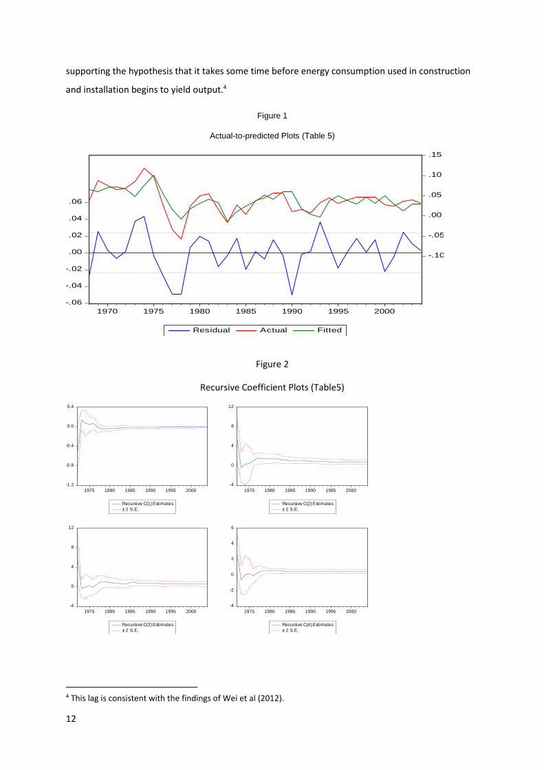
supporting the hypothesis that it takes some time before energy consumption used in construction

and installation begins to yield output.4

Figure 1

Actual-to-predicted Plots (Table 5)

Figure 2

Recursive Coefficient Plots (Table5)

4 This lag is consistent with the findings of Wei et al (2012).

-.06

-.04

-.02

.00

.02

.04

.06

-.10

-.05

.00

.05

.10

.15

1970 1975 1980 1985 1990 1995 2000

Residual Actual Fitted

-1.2

-0.8

-0.4

0.0

0.4

1975 1980 1985 1990 1995 2000

Recursive C(1) Estimates

± 2 S.E.

-4

0

4

8

12

1975 1980 1985 1990 1995 2000


± 2 S.E.

-4

0

4

8

12

1975 1980 1985 1990 1995 2000


± 2 S.E.

-4

-2

0

2

4

6

1975 1980 1985 1990 1995 2000


± 2 S.E.

13

Figure 3

One Step Forecasts (Table5)

Recursive estimation was conducted and stable estimated coefficients are recorded from about

1980 onwards (Figure 2). One-step (Figure 3) and N-step forecasts only identified one outlier in

1990, most likely due to the change in the data set used in that year.

Table 6




cλ 0.006 0.007 0.992 0.329

dlnLt 0.606 0.158 3.835 0.000

dlnEt-2 0.441 0.152 2.905 0.007

dlnGDPSt-1 0.309 0.091 3.383 0.002

DUM1974 0.049 0.017 2.854 0.080

DUM1977 -0.055 0.017 -3.221 0.003

DUM1978 -0.064 0.018 -3.597 0.001

DUM1990 -0.049 0.017 -2.908 0.080


Adjusted R-squared 0.766 S.D. dependent var. 0.034


Breusch-Godfrey Serial Correlation LM Test:

F-statistic 1.319 Prob. F(2,27) 0.284

Obs*R-squared 3.293 Prob. Chi-Square(2) 0.193

.000

.025

.050

.075

.100

.125

.150

-.08

-.04

.00

.04

.08

72 74 76 78 80 82 84 86 88 90 92 94 96 98 00 02 04

One-Step Probability

Recursive Residuals

14

However, it is clear in the actual-to-predicted plots (Figure 1) that there are some significant

deviations in the turbulent mid-1970s. So the model was re-estimated and impulse dummies for

1974, 1977, 1978 and 1990 were found to be significant. The results are reported in Table 6.

Inclusion of impulse dummies has a minor effect on the result, raising the significance of all variables

and lowering the sum of exponents after full adjustment to 1.5. This model fits well (Figure 4).

Figure 4

Figure 5

Recursive Coefficient Plots (Table 6)

-.04

-.02

.00

.02

.04

-.10

-.05

.00

.05

.10

.15

1970 1975 1980 1985 1990 1995 2000

Residual Actual Fitted

-.02

-.01

.00

.01

.02

.03

94 95 96 97 98 99 00 01 02 03 04


± 2 S.E.

0.2

0.4

0.6

0.8

1.0

1.2

94 95 96 97 98 99 00 01 02 03 04


± 2 S.E.

0.0

0.2

0.4

0.6

0.8

1.0

94 95 96 97 98 99 00 01 02 03 04


± 2 S.E.

.0

.1

.2

.3

.4

.5

.6

94 95 96 97 98 99 00 01 02 03 04


± 2 S.E.

.00

.02

.04

.06

.08

.10

94 95 96 97 98 99 00 01 02 03 04


± 2 S.E.

-.10

-.08

-.06

-.04

-.02

.00

94 95 96 97 98 99 00 01 02 03 04


± 2 S.E.

-.12

-.10

-.08

-.06

-.04

-.02

94 95 96 97 98 99 00 01 02 03 04


± 2 S.E.

-.10

-.08

-.06

-.04

-.02

.00

94 95 96 97 98 99 00 01 02 03 04


± 2 S.E.

15

Recursive estimation revealed very stable estimated coefficients (Figure 5). Because there is a lagged

dependent variable in the model, the Breusch-Godfrey Serial Correlation Test was conducted and

there was no evidence that serial correlation was present.

So this preliminary evidence suggests that multi-factor productivity growth, as defined by the ABS

and the PC, has not been the driver of Australian economic growth. This is in line with the findings of

Diewert and Fox (2008) for the US. So, although much more detailed research is required, it has

been quite easy to produce preliminary evidence that increasing returns to scale are important in

determining Australia’s economic growth. In any growing economy that has an imperfectly

competitive industrial structure, we should expect to observe increasing returns to scale.

5. Conclusions

There has been much discussion of Australia’s supposed ‘productivity crisis’ based upon estimates of

multi-factor productivity growth. It has been shown here that it is easy to establish that such

estimates are invalid and preliminary evidence suggests that economies of scale, rather than multi-

factor productivity growth, are likely to have been driving economic growth.

In recent years, what we seemed to have observed is not a productivity crisis but, rather, relatively

high rates of labour productivity growth made possible by well-managed investments in capital

goods and a workforce which has been able to up-skill to take advantage of the capabilities of new

capital goods, particularly computers of all kinds that have enabled massive increases in network

connections and consequent scale advantages. This has resulted in increases in both wages and

profits with a secular shift in the share of GDP towards the latter. Recently, this has all occurred in

the face of a very high Australian dollar. And, of course, it is the pressure imposed by the high

currency that has led to pleas by some industrial groups for government to enact policies that lower

wage costs, purportedly to raise productivity. Yielding to such pressure would be a serious mistake

16

since it would encourage increases in labour intensity in production and provide a disincentive to

innovate through capital investment strategies (Dodgson et.al. (2012)).

From a policy perspective, an economy enjoying economies of scale must be treated differently to

one where it is presumed that disembodied Hicksian technical progress is the dominant driver of

growth. Economics of scale are not just about growth in quantities, they also arise because on

increases in quality. Economic growth is the outcome of a developmental process involving parallel

increases in organisation and complexity (Hausmann and Hidalgo (2011)). As scale increases, the

network structure of the economy expands and the range of goods and services increases. This

increase in diversity leads to increases in value-added in the whole economy. This is particularly true

in the service sector where variety has increased massively as the size of the sector has grown. Much

of this ‘qualitative’ productivity growth is not adequately measured and, thus, not fully reflected in

MFP growth calculations. This is acknowledged in Productivity Commission (2014), p.38, even in

manufacturing. In relation to small scale bakeries it is noted that “the higher quality…may not be

fully reflected in the measures of real value added growth for the subsector, given the challenges in

measuring quality.”

What has been offered here is preliminary econometric evidence. So it is essential that much more

careful research is undertaken to understand fully the role of both static and dynamic economies of

scale and scope in determining Australian economic growth before decisions are made concerning a

new policy designed to enhance productivity growth. Thompson and Webster (2013) point clearly in

the direction that research should go: the interconnected processes of innovation and

entrepreneurship are the ultimate drivers of productivity growth and, therefore, should be at the

core, not the periphery, of econometric studies (Banerjee (2012), Foster (2014)). In the meantime, it

would be useful if the Productivity Commission stopped publishing its highly misleading estimates of

marginal factor productivity growth.

17

References:

Australian Bureau of Statistics (2007) Experimental Estimates of Multifactor Productivity Information

paper Cat. No. 5260.0.55.001, ABS, Canberra.

Banerjee, R. (2012) "Population growth and Endogenous Technological Change: Australian Economic

Growth in the Long Run", Economic Record, vol. 88, pp. 214-228.

Cohen, A.J. and Harcourt, C.G. (2003). “Whatever Happened to the Cambridge Capital Theory

Controversies?” Journal of Economic Perspectives, vol. 17, 1, pp. 199–214

Cutler, T. (2008) Venturous Australia Report, Cutler & Company Pty Ltd, Melbourne.

Bloom, N., Genakos, C., Sadun, R. and van Reenen, J. (2012), ‘Management practices across firms

and countries’, National Bureau of Economic Research Working Papers, no 17850.

DCITA (2005) “Estimating aggregate productivity growth for Australia: The role of information and

communications technology.” An Occasional Economic Paper, Commonwealth of Australia,

September

Diewert, W. Erwin & Fox, Kevin J. (2008). "On the estimation of returns to scale, technical progress

and monopolistic mark-ups," Journal of Econometrics, vol. 145(1-2), pp. 174-193.

Dodgson, M., Hughes, A., Foster, J. and and Metcalfe, J.S (2011) “Systems thinking, market failure

and the development of innovation policy: the case of Australia.” Research Policy, vol. 40, issue 9,

pp. 1145-1156.

Felipe, J. and McCombie, J.S.L. (2013) The Aggregate Production Function And The Measurement Of

Technical Change: ‘Not Even Wrong’ Edward Elgar: Cheltenham.

Foster, J. (2014) “Energy, knowledge and economic growth.” Journal of Evolutionary Economics,

vol.24, pp.209-238.

Hausmann, R. and Hidalgo, C. (2011). "The network structure of economic output," Journal of

Economic Growth, vol. 16, issue 4, pp. 309-342.

Parham, D. (2013). “Australia's Productivity: Past, Present and Future.” Australian Economic Review,

vol. 46, Issue 4, pp. 462–472.

Productivity Commission (2013) “Capital Utilisation in the Mining Industry.” Productivity Update,

Commonwealth of Australia, May.

Productivity Commission (2014) “Insights from recent productivity research – productivity in

manufacturing.” Productivity Update, Commonwealth of Australia, April.

Solow, R.M. (1957) "Technical Change and the Aggregate Production Function". Review of Economics

and Statistics, vol. 39, issue 3, pp. 312–320.

18

Snooks, G. (1994). Portrait of the Family within the Total Economy: a Study in Long-run dynamics,

Australia, 1778-1990.Cambridge University Press: Cambridge.

Thomson, R. and Webster, E. (2013). “Innovation and Productivity.” Australian Economic Review,

vol. 46, issue 4, pp. 483–488.

Wei, H., Loughton, B., Xiang, J and Zhang, R. (2012) “Getting Measures of Capital Services Right:

Accounting for Capital Utilisation in the Mining Industry.” Paper prepared for the 41th Annual

Conference of Economists, 8-12 July 2012, Melbourne, Australia.

Data Sources

GDP

The annual gross domestic product series from 1965 to 1990 is taken from Snooks (1994) Table 7.9

p. 181. The remaining 14 years of data are obtained from the ABS national accounts given in current

prices but converted to constant prices by chaining the relevant ABS deflator with the Snooks (1994)

deflator.

Capital Stock

The annual capital stock index used is taken from DCITA (2005), Table 1, p.15.

Labour

The annual total labour hours index used is taken from DCITA (2005), Table 1, p.15.

Energy

The BP Statistical Review of World Energy contains annual data on the production and consumption

of coal, oil, gas, hydroelectricity and other renewables in Australia since 1965, courtesy of the

International Energy Agency.

Multi-Factor Productivity Growth

ABS Multi-Factor Productivity and the Diewert-Lawrence Total Factor Productivity Estimates are

drawn from DCITA (2005), Table 1, p.15

the australian multi-factor productivity growth illusion · 1 the australian multi-factor...

Documents