the application of stata's multiple imputation techniques to

The Application of STATA’s Multiple Imputation

Techniques to Analyze a Design of Experiments

with Multiple Responses

STATA Conference - San Diego 2012Clara Novoa, Ph.D., Bahram Aiabanpour, Ph.D.,

Suleima AlkusariTexas State University - San Marcos, TX, USA

Ingram School of Engineering

Novoa et al. (Texas State University) STATA Conference 2012 1 / 29

Overview

Introduction

Previous workMotivation

Multiple Imputation Methodology

Multiple Imputation in STATA

Results

Conclusions


Introduction

Plasma Cutting Technology


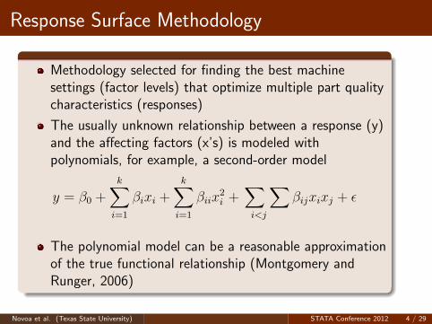
Response Surface Methodology

Methodology selected for finding the best machinesettings (factor levels) that optimize multiple part qualitycharacteristics (responses)

The usually unknown relationship between a response (y)and the affecting factors (x’s) is modeled withpolynomials, for example, a second-order model

y = β0 +k∑

i=1

βixi +k∑

i=1

βiix2i +

∑i<j

∑βijxixj + ε

The polynomial model can be a reasonable approximationof the true functional relationship (Montgomery andRunger, 2006)


Response Surface Methodology (continuation)

Experimental design permits the collection of data forthe response variable at different levels of theindependent variables

Least squares method permits the estimation of theparameters, β ’s, in the approximating polynomials

Linear/non-linear optimization techniques permits thefinding of an optimum point (x∗1, x

∗2, ..., x

∗k) and an

optimal response value (y∗)


Experimental Design - Part Geometry

All cuts were made on stainless steel sheet metal of 0.25 inchthickness


Experimental Design - Factors and Levels

Factor Name Low Medium High UnitsA Current 40 60 80 AmpsB Pressure 60 75 90 PsiC Cut Speed 10 55 100 IpmD Torch height 0.1 0.2 0.3 InchE Tool type *1 A B CF Slower on curve 0 2 4G Cut direction Vertical Horizontal

(G 0) (G 1)

*1 In experiment with missing values level names were (E 1, E 2, E 3)

*1 In experiment with imputed values names names were (E 0, E 1, E 2)


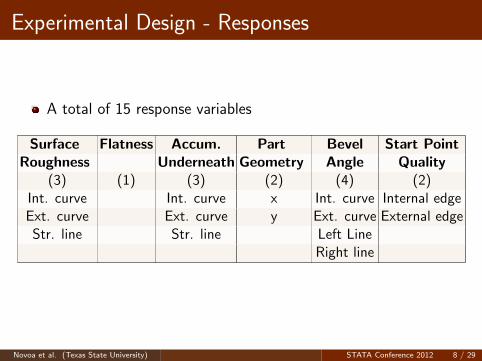
Experimental Design - Responses

A total of 15 response variables

Surface Flatness Accum. Part Bevel Start PointRoughness Underneath Geometry Angle Quality

(3) (1) (3) (2) (4) (2)Int. curve Int. curve x Int. curve Internal edgeExt. curve Ext. curve y Ext. curve External edgeStr. line Str. line Left Line

Right line


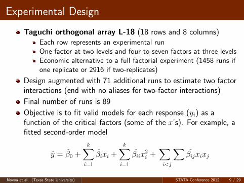
Experimental Design

Taguchi orthogonal array L-18 (18 rows and 8 columns)Each row represents an experimental runOne factor at two levels and four to seven factors at three levelsEconomic alternative to a full factorial experiment (1458 runs ifone replicate or 2916 if two-replicates)

Design augmented with 71 additional runs to estimate two factorinteractions (end with no aliases for two-factor interactions)

Final number of runs is 89

Objective is to fit valid models for each response (yi) as afunction of the critical factors (some of the x’s). For example, afitted second-order model

y = β0 +k∑

i=1

βixi +k∑

i=1

βiix2i +

∑i<j

∑βijxixj


Optimization using Desirability Functions -

Derringer and Suich (1980)

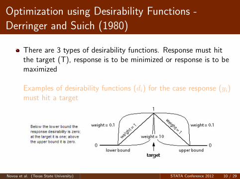
There are 3 types of desirability functions. Response must hitthe target (T), response is to be minimized or response is to bemaximized

Examples of desirability functions (di) for the case response (yi)must hit a target


Desirability Function - Target is Best

di(Yi(x)) =

0 Yi(x) < Li(Yi(x)−Li

Ti−Li

)sLi < Yi(x) < Ti(

Yi(x)−Ui

Ti−Ui

)tLi < Yi(x) < Ti

0 Yi(x) > Ui

The desirability function ”target is best” transforms theresponse values to values between 0 and 1, zero if below alower bound (L) or one if above an upper bound (U)

The shape of the desirability function is determined by thevalues of the weight parameters s and t (function exponents)

Settings for independent variables or factors affect thepredicted response and the desirability function values


Optimizing the Overall Desirability

maximize

D = (n∏

i=1

di(Yi(x))wi)

1∑ni=1

wi

subject to

Low ≤ x ≤ High

This is a non-linear deterministic optimization model with objective function tomaximize the overall desirability. Weights wi represent the importance given toresponse yi

x is the vector of model decision variables corresponding to the non-categoricalexperimental factors (current, pressure, cut speed, torch height, and slower oncurves)

Constraints in the model say that decision variables x’s must to take values withinthe experimented region (Low-High). Categorical factors tool type and cutdirection are fixed to each one of their 6 possible levels. Thus, six differentoptimization models need to be solved in this study


Research Motivation

43 experimental conditions had missed responses (36 had allresponses missing and other 7 had some responses missing)

Analysis of the experiment done through general linearregression model (GLM) ignoring the missing responses

Is multiple imputation (MI) an effective method forcompleting and analyzing this experimental design?


Multiple Imputation (MI)

Method proposed by Rubin (1987). It is a simulation-basedapproach for analyzing incomplete data (Manchenko, 2010)

Each missing value is replaced with a random sample ofsimulated values that represent the uncertainty about the rightvalue (Rubin, 1987)

User specifies the size of the random sample (number ofimputations to add)

Includes 3 steps: imputing, conducting analysis with eachcomplete set of data, and analyzing aggregate results

Variances of the parameter estimates are estimated moreaccurately than in single-imputation reducing the type I error

In contrast to single-imputation, MI permits to estimate theimpact of missing information on parameter estimation(McKnight, et al., 2007)


MI in STATA 11 - Multiple Imputation Control

Panel

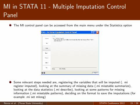
The MI control panel can be accessed from the main menu under the Statistics option

Some relevant steps needed are, registering the variables that will be imputed (. miregister imputed), looking at the summary of missing data (.mi misstable summarize),looking at the data statistics (.mi describe), looking at some patterns for missinginformation (.mi misstable patterns), deciding on the format to save the imputations (forexample .mi set mlong)


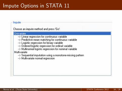
Impute Options in STATA 11


Impute Command - Example

In this example, the number of imputations for each missing value, m, is 5 and theimputation method selected was predictive mean matching (pmm)


Impute Options - Predictive Mean Matching

(pmm)

Preferred to linear regression when the normality of theunderlying model is suspect

Introduced by Little (1988) based on Rubin (1986)

Prediction of linear regression is used as a distance measure toform the set of nearest neighbors or donors for the imputation

Randomly draws a value from the set of nearest neighbors toimpute the missing value

By drawing from the observed data ppm preserves the originaldistribution of the observed values

Estimates of the model parameters are simulated from their jointposterior distribution


Estimate Command - Example - Output 1

The first time the command mi estimate was invoked, a regression (regress) fornewFlatness as dependent variable and all the possible terms in a second orderpolynomial model on the factors (current, pressure, cut speed torch height, slow oncurve, tool type and cut direction) was performed. Quadratic terms and second orderinteractions were included except those involving categorical variables

By performing iteratively the command mi estimate, we eliminated from the model thenon-significant factors one at a time until obtaining a final regression model with onlysignificant factors for each response


Estimate Command - Example - Output 2

RVI = Relative variance increase due to non-responseFMI = Fraction of missing informationThe smaller the RVI and FMI values the betterRVI can be greater than 1

Relative efficiency value, the closer to 1 the better


Deterministic Optimization Model

The multi-response non-linear optimization model was laid outin Excel

Risk Solver Platform (RSP) software from Frontline Systems wasused for the optimization step.

The optimization technique used by RSP to solve the non-linearnon-smooth optimization problem is genetic algorithms (GA)

Solve times were less than 1 minute 43 seconds in all runs andthe mean was 55.74 seconds


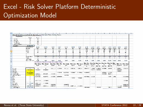
Excel - Risk Solver Platform Deterministic

Optimization Model


Numerical Results

Experiment ExperimentFactor no imputation with MICurrent 80 80Pressure 90 90Cut Speed 55 65Torch height 0.3 0.3Slower on Curves 0.4 0Tool Type Third tool Second toolCut direction Horizontal Horizontal


Conclusions and Further Research

MI under STATA proved to be effective to analyze the plasmacutting experiment with missing valuesAfter MI, it was discovered that a setting with slightly higherspeeds do not negatively affect response variables and overalldesirabilityMI reports on the variability of the estimates of the regressioncoefficients. This variability may be included in a stochasticsimulation optimization model that Risk Solver Platform(RSP) can solve

The stochastic optimization model objective function is now tominimize the expected overall desirability under the sameconstraints as in the deterministic optimization modelβ’s in the regression models are now random variables with agiven mean and standard error. Desirability’s will depend onresponses which will be a function of the factors (x’s) and therealizations for the β’s


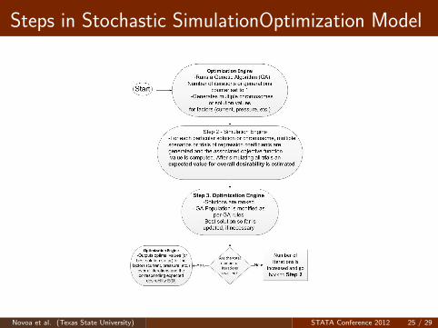
Steps in Stochastic SimulationOptimization Model


References

1. Asiabanpour, B., Vejandla, D. T., Jimenez, J., and Novoa, C., 2009, Optimizing theAutomated Plasma Cutting Process by Design of Experiments, International Journal ofRapid Manufacturing 1(1), 19−40.

2. Vejandla, D. T., 2009, Optimizing the Automated Plasma Cutting Process by Designof Experiments, Masters Thesis, Texas State University, Department of EngineeringTechnology.

3. Montgomery, D. C., 2001, Design and Analysis of Experiments, 5th Edition, JohnWiley & Sons, Inc., New York.

4. Montgomery, D.C., Runger, G.C., 2006, Applied Statistics and Probability forEngineers, 4th Edition, John Wiley & Sons, Inc., New York.

5. Godolphin, J. D., 2006, Reducing the Impact of Missing Values in FactorialExperiments Arranged in Blocks, Quality and Reliability Engineering International 23,669−682.

6. Yuan, Y. C., Multiple Imputation for Missing Data: Concepts and New Development(version 9.0), SAS Institute Inc., Rockville, MD.

7. Castillo, E. D., Montgomery, D., and McCarville, D., 1996, Modified DesirabilityFunctions for Multiple Response Optimization, Journal of Quality Technology, 28(3),337−345.

8. NIST−SEMATECH, 2003, Section 5.5.3.2.2: Multiple Responses: The DesirabilityApproach in e-Handbook of Statistical Methods, Engineering Statistics Handbook.Online. http://www.itl.nist.gov/div898/handbook/pri/section5/pri5322.htm. Last dateaccessed Jan 16, 2012.


References - Continuation

9. ArtilesLeon, N., NovoaRamirez, C. M. & Domenech, C., 1995. Improving fabricfinishing through experimental design, ASQC 49th Annual Quality Congress Proceedings,USA, pp. 952-961.

10. Koller-Meinfelder, F., 2009. Analysis of Incomplete Survey Data MultipleImputation via bayesian Bootstrap Predictive Mean Matching, Germany:Otto-Friedrich-Universitat Bamberg. Online. Last date Accessed July 23, 2012.

11. Manchenko, Y., 2010. Mutipleimputation using Stata’s mi command. Online.http://www.stata.com/meeting/boston10/boston10 marchenko.pdf. Last date accessedJuly 23, 2012.

12. McKnight, P. E., McKnight, K. M., Sidani, S. & Fuigueredo, J. A., 2007. MissingData A Gentle Introduction. 1st ed. N.Y.: The Guilford Press.

13. Mealli, F. & Rubin, D. B., 2002. Assumptions when Analyzing RandomizedExperiments with Noncompliance and Missing Outcomes. Health Services & OutcomesResearch Methodology, Volume 3, pp. 225−232.

14. Rubin, D. B., 1987. Multiple Imputation for Nonresponse in Surveys. 1st ed. NewYork: Wiley.

15. Rubin, D. B., 1996. Multiple imputation after 18 years (with discussion). Journal ofthe American Statistical Association, 91(434), pp. 473−489.

16. STATA. Multiple imputation for missing data. Online.http://www.stata.com/stata11.mi.html. Last Date Accessed July 23, 2012.


References - Continuation

17. Schafer, J. The multiplie imputation frequently asked page. Online. Available at:http://sites.stat.psu.edu/jls/mifaq.html.Last Date July 23, 2012

18. Verbeke, G. & Mohenberghs, G., 2000. Linear mixed models for longitudinal data.New York: SpringerVerlag.

19. Wayman, J. C., 2003, Multiple Imputation For Missing Data: What Is It And HowCan I Use It? , Annual Meeting of The American Education Research Association,Chicago, IL., available athttp://www.csos.jhu.edu/contact/staff/jwayman pub/wayman multimp aera2003.pdf(last date accessed Jan 16, 2012)


Questions


the application of stata's multiple imputation techniques to

Documents