the application of space-filling curves to the storage and retrieval of multi-dimensional data
TRANSCRIPT

The Application of Space-�lling Curves to
the Storage and Retrieval of Multi-dimensional
Data
by
Jonathan Lawder
A thesis submitted in the ful�llment of the requirements
for the degree of
Doctor of Philosophy
in the
University of London
December 1999
Birkbeck College
Viva Voce : 30 March 2000
Professor D McGregor, Dr D A Cohen

ii
ABSTRACT
Indexing of multi-dimensional data has been the focus of a considerable amount of research
e�ort over many years but no generally agreed paradigm has emerged to compare with
the impact of the B-Tree, for example, on the indexing of one-dimensional data. At the
same time, the need for e�cient methods is ever more important in an environment where
databases become larger and more complex in their structures.
Mapping multi-dimensional data to one dimension, thus enabling one-dimensional ac-
cess methods to be exploited, has been suggested in the literature but for the most part
interest has been con�ned to the Z-order curve. The possibility of using other curves, such
as the Hilbert and Gray-code curves, whose characteristics di�er from those of the Z-order
curve, has also been suggested.
In this thesis we design and implement a working �le store which is underpinned by the
principle of mapping multi-dimensional data to one of a variety of space-�lling curves and
their variants. Data is then indexed using a B+ Tree which remains compact, regardless
of the volume and number of dimensions. The implementation has entailed developing
algorithms for mapping data to one dimension and, most importantly, developing algo-
rithms to facilitate the querying of data in a exible way. We focus on the Hilbert curve
but also consider other curves and propose new alternative algorithms for querying data
mapped to the Z-order curve.
The current implementation accommodates data in up to sixteen dimensions but the
approach is generic and not limited to this number. We report on preliminary testing of
the implemetation, which provides very encouraging results. We also undertake a brief
exploration of the application of space-�lling curves to the indexing of spatial data.

iii
This thesis is dedicated to my mother and father.
�Cetrdeset mi je godina, ru�zno doba: �covjek je jo�s mlad da bi imao �zelja a ve�c
star da ih ostvaruje.
from Dervi�s i smrt
by Me�sa Selimovi�c
This volume is a compact and abridged version of a thesis submitted in December 1999
in ful�lment of the requirements of the University of London for the degree of Doctor of
Philosophy and amended following the Viva in March 2000. It di�ers from the copies held
in the libraries of the University of London and Birkbeck College in formatting and in its
omission of Appendices E and F.
c J.K.Lawder 2000. The copyright of this thesis rests with the author and no quotation
from it or information derived from it may be published without the prior written consent
of the author.

iv
CONTENTS
1. Introduction : : : : : : : : : : : : : : : : : : : : : : : : : : : : : : : : : : : : : 1
1.1 Background . . . . . . . . . . . . . . . . . . . . . . . . . . . . . . . . . . . . 1
1.2 Approach to Data Organization Developed in the Thesis . . . . . . . . . . . 2
1.3 Problems with Existing Multi-dimensional Indexing Methods . . . . . . . . 3
1.4 The Major Contribution of this Thesis . . . . . . . . . . . . . . . . . . . . . 5
1.5 Review of the Work Undertaken . . . . . . . . . . . . . . . . . . . . . . . . 5
1.6 Structure of the Thesis . . . . . . . . . . . . . . . . . . . . . . . . . . . . . . 7
2. Previous Work : : : : : : : : : : : : : : : : : : : : : : : : : : : : : : : : : : : : 9
2.1 Mapping to Space-�lling Curves . . . . . . . . . . . . . . . . . . . . . . . . . 9
2.1.1 The Hilbert Curve . . . . . . . . . . . . . . . . . . . . . . . . . . . . 9
2.1.2 The Z-order Curve . . . . . . . . . . . . . . . . . . . . . . . . . . . . 11
2.1.3 The Gray-code Curve . . . . . . . . . . . . . . . . . . . . . . . . . . 11
2.2 The Application of Space-�lling Curves to Indexing Multi-dimensional Data 11
2.2.1 Clustering Properties of Space-�lling Curves . . . . . . . . . . . . . . 11
2.2.2 The Utilization of Space-�lling Curves . . . . . . . . . . . . . . . . . 13
2.2.2.1 The Hilbert Curve . . . . . . . . . . . . . . . . . . . . . . . 13
2.2.2.2 The Z-order Curve . . . . . . . . . . . . . . . . . . . . . . . 15
2.2.2.3 The Gray-code Curve . . . . . . . . . . . . . . . . . . . . . 17
2.3 Other Multi-dimensional Storage Structures . . . . . . . . . . . . . . . . . . 17
2.3.1 Recent Methods . . . . . . . . . . . . . . . . . . . . . . . . . . . . . 19
2.4 Current Commercially Available Software . . . . . . . . . . . . . . . . . . . 21
2.5 B-Trees . . . . . . . . . . . . . . . . . . . . . . . . . . . . . . . . . . . . . . 22
3. Space-�lling and Related Curves and their Application : : : : : : : : : : 23
3.1 Introduction . . . . . . . . . . . . . . . . . . . . . . . . . . . . . . . . . . . . 23
3.2 The Origin of Space-�lling Curves . . . . . . . . . . . . . . . . . . . . . . . 24
3.3 The De�nition of a Space-�lling Curve . . . . . . . . . . . . . . . . . . . . . 24
3.4 The Construction of Hilbert Space-�lling Curves . . . . . . . . . . . . . . . 25
3.4.1 The Hilbert Curve in 2 Dimensions . . . . . . . . . . . . . . . . . . . 25
3.4.2 The Hilbert Curve in Higher Dimensions . . . . . . . . . . . . . . . . 28
3.5 Binary Representation of the Hilbert Curve . . . . . . . . . . . . . . . . . . 28
3.6 A Tree Representation of Space-�lling Curves . . . . . . . . . . . . . . . . . 32
3.7 Alternatives to Space-�lling Curves . . . . . . . . . . . . . . . . . . . . . . . 33
3.7.1 The Z-order Curve . . . . . . . . . . . . . . . . . . . . . . . . . . . . 35
3.7.2 The Gray-code Curve . . . . . . . . . . . . . . . . . . . . . . . . . . 39
3.7.3 The Scan and Snake Curves . . . . . . . . . . . . . . . . . . . . . . . 45
3.7.4 Other Curves . . . . . . . . . . . . . . . . . . . . . . . . . . . . . . . 47
3.8 The Application of Space-�lling Curves . . . . . . . . . . . . . . . . . . . . 48
3.8.1 Use of Approximations of Space-�lling Curves . . . . . . . . . . . . . 48
3.8.2 The Choice of Curve . . . . . . . . . . . . . . . . . . . . . . . . . . . 48
3.8.3 Partitioning of Data . . . . . . . . . . . . . . . . . . . . . . . . . . . 49

Contents v
4. Techniques for Mapping to and from Space-�lling Curves : : : : : : : : 51
4.1 Introduction . . . . . . . . . . . . . . . . . . . . . . . . . . . . . . . . . . . . 51
4.2 Summary of Alternative Mapping Techniques for the Hilbert Curve . . . . . 52
4.3 State Diagrams . . . . . . . . . . . . . . . . . . . . . . . . . . . . . . . . . . 53
4.3.1 Generating State Diagrams by Hand . . . . . . . . . . . . . . . . . . 54
4.3.2 Bially's Algorithm for Creating a State Diagram Generator Table . . 54
4.3.3 State Diagram Generator Table for the Hilbert Curve . . . . . . . . 62
4.3.4 Variations to State Diagram Generator Tables for the Hilbert Curve 67
4.3.5 State Diagram Generator Tables for Discontinuous Curves . . . . . . 68
4.3.5.1 The Z-order Curve . . . . . . . . . . . . . . . . . . . . . . . 68
4.3.5.2 Moore's Curve . . . . . . . . . . . . . . . . . . . . . . . . . 68
4.3.5.3 The Gray-code Curves . . . . . . . . . . . . . . . . . . . . . 70
4.3.6 Production of State Diagrams from Generator Tables . . . . . . . . 70
4.3.7 State Diagram Growth Rate . . . . . . . . . . . . . . . . . . . . . . . 74
4.3.7.1 The Hilbert Curve . . . . . . . . . . . . . . . . . . . . . . . 74
4.3.7.2 Discontinuous Curves . . . . . . . . . . . . . . . . . . . . . 77
4.4 Mapping to the Hilbert Curve Using the State Diagram Generator Table . . 78
4.5 Mapping to the Hilbert Curve by Calculation . . . . . . . . . . . . . . . . . 79
5. Algorithms for Mapping to and from Space-�lling Curves : : : : : : : : 81
5.1 Algorithm for Hilbert Curve Mapping using a State Diagram . . . . . . . . 81
5.2 Algorithm for Hilbert Curve Mapping using a State Diagram Generator
Table . . . . . . . . . . . . . . . . . . . . . . . . . . . . . . . . . . . . . . . 83
5.3 Algorithm for Hilbert Curve Mapping using Calculation . . . . . . . . . . . 85
5.4 Algorithms for the Z-order Curve . . . . . . . . . . . . . . . . . . . . . . . . 86
5.5 Algorithms for the Gray-code Curve . . . . . . . . . . . . . . . . . . . . . . 88
5.6 Complexity of the Mapping Techniques . . . . . . . . . . . . . . . . . . . . 89
5.7 Conclusions . . . . . . . . . . . . . . . . . . . . . . . . . . . . . . . . . . . . 90
6. Algorithms for Querying Data Mapped to Space-�lling Curves : : : : : 91
6.1 Introduction . . . . . . . . . . . . . . . . . . . . . . . . . . . . . . . . . . . . 91
6.2 Types of Query . . . . . . . . . . . . . . . . . . . . . . . . . . . . . . . . . . 91
6.3 Querying Data Mapped to Space-�lling Curves . . . . . . . . . . . . . . . . 92
6.4 The Hilbert Curve . . . . . . . . . . . . . . . . . . . . . . . . . . . . . . . . 98
6.4.1 Introductory Examples . . . . . . . . . . . . . . . . . . . . . . . . . . 98
6.4.2 Querying Algorithms . . . . . . . . . . . . . . . . . . . . . . . . . . . 99
6.4.2.1 Range Queries . . . . . . . . . . . . . . . . . . . . . . . . . 110
6.4.2.1.1 Overview of the Algorithm . . . . . . . . . . . . . 110
6.4.2.1.2 Algorithms which Utilize State Diagrams . . . . . 112
6.4.2.1.3 Application Of The Algorithms In Higher Dimen-
sions . . . . . . . . . . . . . . . . . . . . . . . . . 119
6.4.2.2 Partial Match Queries . . . . . . . . . . . . . . . . . . . . . 120
6.5 The Z-order Curve . . . . . . . . . . . . . . . . . . . . . . . . . . . . . . . . 121
6.5.1 Bit Manipulation Querying Algorithms . . . . . . . . . . . . . . . . 121
6.5.1.1 Lowest and Highest Matches . . . . . . . . . . . . . . . . . 121
6.5.1.2 Range Queries . . . . . . . . . . . . . . . . . . . . . . . . . 121
6.5.1.3 Bit Manipulation Partial Match Query Algorithm . . . . . 126
6.5.2 Tree-descent Range Query Algorithm . . . . . . . . . . . . . . . . . 129
6.6 Complexity of the Algorithms . . . . . . . . . . . . . . . . . . . . . . . . . . 130
6.6.1 Tree Descent Algorithms . . . . . . . . . . . . . . . . . . . . . . . . . 130
6.6.2 Z-order Bit Manipulation Algorithms . . . . . . . . . . . . . . . . . 131

Contents vi
7. File Implementation : : : : : : : : : : : : : : : : : : : : : : : : : : : : : : : : 132
7.1 Design Summary . . . . . . . . . . . . . . . . . . . . . . . . . . . . . . . . . 132
7.1.1 Curves used in the Mappings . . . . . . . . . . . . . . . . . . . . . . 132
7.1.2 Number of Dimensions . . . . . . . . . . . . . . . . . . . . . . . . . . 133
7.1.3 Order of Curve . . . . . . . . . . . . . . . . . . . . . . . . . . . . . . 133
7.1.4 Storage of Data During the Execution of Computer Programs . . . . 133
7.1.5 The Data File . . . . . . . . . . . . . . . . . . . . . . . . . . . . . . . 134
7.1.6 The Index . . . . . . . . . . . . . . . . . . . . . . . . . . . . . . . . . 134
7.1.7 Main Memory Bu�er . . . . . . . . . . . . . . . . . . . . . . . . . . . 134
7.1.8 Ancillary Files . . . . . . . . . . . . . . . . . . . . . . . . . . . . . . 135
7.1.9 Query Execution Strategy . . . . . . . . . . . . . . . . . . . . . . . . 135
7.2 The Application Interface . . . . . . . . . . . . . . . . . . . . . . . . . . . . 135
7.3 Use and Compatibility with other TriStarp Group Software . . . . . . . . . 136
7.4 Implementation Details . . . . . . . . . . . . . . . . . . . . . . . . . . . . . 137
7.4.1 Storing Data as derived-keys . . . . . . . . . . . . . . . . . . . . . . 138
7.4.1.1 Ordered Data . . . . . . . . . . . . . . . . . . . . . . . . . 138
7.4.1.2 Unordered Data . . . . . . . . . . . . . . . . . . . . . . . . 139
7.4.2 Storing Data in Coordinate Format . . . . . . . . . . . . . . . . . . . 139
7.4.2.1 Ordered Data . . . . . . . . . . . . . . . . . . . . . . . . . 139
7.4.2.2 Unordered Data . . . . . . . . . . . . . . . . . . . . . . . . 140
7.4.3 Redistribution of Data Stored in Coordinate Format and in Sort Order140
7.4.3.1 Page Splitting . . . . . . . . . . . . . . . . . . . . . . . . . 141
7.4.3.2 Moving Data to Underpopulated Pages . . . . . . . . . . . 141
7.4.3.3 General Procedure for Dealing with Underpopulated Pages 142
7.5 Potential Variations to the Indexing Implementation . . . . . . . . . . . . . 143
7.5.1 Indexing Intervals . . . . . . . . . . . . . . . . . . . . . . . . . . . . 143
7.5.2 Adjusting Page-key Values to In uence Page Shape . . . . . . . . . 144
7.5.3 The Application of B�-Tree Concepts . . . . . . . . . . . . . . . . . 145
7.6 Concluding Remarks . . . . . . . . . . . . . . . . . . . . . . . . . . . . . . . 146
8. Comparison with other File Organization Methods : : : : : : : : : : : : : 147
8.1 The Grid File . . . . . . . . . . . . . . . . . . . . . . . . . . . . . . . . . . . 147
8.1.1 The Index . . . . . . . . . . . . . . . . . . . . . . . . . . . . . . . . . 147
8.1.2 Management of the Storage of Data . . . . . . . . . . . . . . . . . . 150
8.1.2.1 Page Splitting . . . . . . . . . . . . . . . . . . . . . . . . . 150
8.1.2.2 Underpopulated Pages . . . . . . . . . . . . . . . . . . . . . 151
8.1.3 Query Execution . . . . . . . . . . . . . . . . . . . . . . . . . . . . . 151
8.2 The BANG File . . . . . . . . . . . . . . . . . . . . . . . . . . . . . . . . . . 153
8.2.1 The Index . . . . . . . . . . . . . . . . . . . . . . . . . . . . . . . . . 153
8.2.2 Management of the Storage of Data . . . . . . . . . . . . . . . . . . 155
8.2.2.1 Overpopulated Pages . . . . . . . . . . . . . . . . . . . . . 155
8.2.2.2 Underpopulated Pages . . . . . . . . . . . . . . . . . . . . . 155
8.2.3 Query Execution . . . . . . . . . . . . . . . . . . . . . . . . . . . . . 156
9. Indexing of Spatial Data using Space-�lling Curves : : : : : : : : : : : : 157
9.1 Introduction . . . . . . . . . . . . . . . . . . . . . . . . . . . . . . . . . . . . 157
9.2 The Representation of Spatial Data . . . . . . . . . . . . . . . . . . . . . . . 157
9.3 Querying Spatial Data . . . . . . . . . . . . . . . . . . . . . . . . . . . . . . 158
9.3.1 Overlap Queries . . . . . . . . . . . . . . . . . . . . . . . . . . . . . 158
9.3.2 Containment Queries . . . . . . . . . . . . . . . . . . . . . . . . . . . 159
9.4 Implementation and Testing . . . . . . . . . . . . . . . . . . . . . . . . . . . 159

Contents vii
10.Results of Some Preliminary Testing : : : : : : : : : : : : : : : : : : : : : : 160
10.1 Test Parameters . . . . . . . . . . . . . . . . . . . . . . . . . . . . . . . . . 160
10.2 Tests Carried Out and their Results . . . . . . . . . . . . . . . . . . . . . . 162
10.2.1 Data File Creation . . . . . . . . . . . . . . . . . . . . . . . . . . . . 162
10.2.2 Query Execution . . . . . . . . . . . . . . . . . . . . . . . . . . . . . 163
10.3 Discussion and Conclusions . . . . . . . . . . . . . . . . . . . . . . . . . . . 166
10.4 Spatial Data . . . . . . . . . . . . . . . . . . . . . . . . . . . . . . . . . . . 167
11.Conclusions : : : : : : : : : : : : : : : : : : : : : : : : : : : : : : : : : : : : : : 168
Bibliography : : : : : : : : : : : : : : : : : : : : : : : : : : : : : : : : : : : : : 172
A. Symbols : : : : : : : : : : : : : : : : : : : : : : : : : : : : : : : : : : : : : : : : 179
B. The Hilbert Curve : : : : : : : : : : : : : : : : : : : : : : : : : : : : : : : : : 180
B.1 The State Diagram Approach { Some Examples . . . . . . . . . . . . . . . . 180
B.2 Calculated Hilbert Curve Mappings . . . . . . . . . . . . . . . . . . . . . . 189
C. Moore's Curve: Our Variation : : : : : : : : : : : : : : : : : : : : : : : : : : 194
D. The Gray-code Curve : : : : : : : : : : : : : : : : : : : : : : : : : : : : : : : 197
D.1 Creation of State Diagram Generator Tables . . . . . . . . . . . . . . . . . . 197
D.2 Some Examples of State Diagram Generator Tables . . . . . . . . . . . . . . 199
E. Source Code for Generation of State Diagrams : : : : : : : : : : : : : : : 206
F. Source Code for Data Management Implementation : : : : : : : : : : : : 207
Index of de�nitions . . . . . . . . . . . . . . . . . . . . . . . . . . . . . . . . . . . 208

viii
LIST OF FIGURES
1.1 Example Showing a Partitioning of Data Mapped to the Hilbert curve in 2
Dimensions . . . . . . . . . . . . . . . . . . . . . . . . . . . . . . . . . . . . 6
2.1 Example Partitioning and Index in the R-Tree in 2 Dimensions . . . . . . . 14
2.2 The Application of the Quad Tree to an Image . . . . . . . . . . . . . . . . 16
2.3 Taxonomy of Data Organization Methods from [GG98] . . . . . . . . . . . . 18
2.4 Partitioning within the Pyramid-Technique . . . . . . . . . . . . . . . . . . 21
3.1 Approximations of the Hilbert Curve in 2 Dimensions . . . . . . . . . . . . 24
3.2 First Order Hilbert Curve: Mapping between Sub-squares and Sub-intervals
in 2 Dimensions . . . . . . . . . . . . . . . . . . . . . . . . . . . . . . . . . . 26
3.3 Second Order Hilbert Curve in 2 Dimensions . . . . . . . . . . . . . . . . . 27
3.4 Third and Fourth Order Hilbert Curves in 2 Dimensions . . . . . . . . . . . 27
3.5 Hilbert First Order Curves in 3 Dimensions . . . . . . . . . . . . . . . . . . 29
3.6 Connecting 3-Dimensional First Order Hilbert Curves . . . . . . . . . . . . 30
3.7 An `Unsuitable' 3-Dimensional First Order Curve . . . . . . . . . . . . . . . 30
3.8 Second Order Hilbert Curve: Mapping between Coordinates and Sub-interval
Sequence Numbers in 2 Dimensions . . . . . . . . . . . . . . . . . . . . . . . 31
3.9 The Tree Representation of the Third Order Hilbert Curve in 2 Dimensions 34
3.10 Approximations of the Z-order Curve in 2 Dimensions . . . . . . . . . . . . 36
3.11 Calculation of the Z-order derived-key of a Point . . . . . . . . . . . . . . . 37
3.12 Alternative Approximations of the Z-order Curve in 2 Dimensions . . . . . 38
3.13 The Sequence of Gray-codes of Length 4 . . . . . . . . . . . . . . . . . . . . 40
3.14 The Gray-codeF Curve in 2 Dimensions (after Faloutsos) . . . . . . . . . . 41
3.15 The Gray-codeF Curve in 3 Dimensions (after Faloutsos) . . . . . . . . . . 42
3.16 The Gray-codeA Curve in 2 Dimensions . . . . . . . . . . . . . . . . . . . . 43
3.17 The Gray-codeA Curve in 3 Dimensions . . . . . . . . . . . . . . . . . . . . 44
3.18 The Gray-codeB Curve in 2 Dimensions . . . . . . . . . . . . . . . . . . . . 45
3.19 The Gray-codeB Curve in 3 Dimensions . . . . . . . . . . . . . . . . . . . . 46
3.20 The 2-dimensional `Scan' and `Snake' Curves in 2 Dimensions . . . . . . . . 47
3.21 Approximations of a Single-State Curve in 2 Dimensions . . . . . . . . . . . 48
3.22 Example Showing a Partitioning of Data Mapped to the Hilbert Curve in
2 Dimensions . . . . . . . . . . . . . . . . . . . . . . . . . . . . . . . . . . . 50
4.1 A State Diagram for the Hilbert Curve in 2 Dimensions . . . . . . . . . . . 58
4.2 Second Order 3-dimensional Hilbert Curve Implied by our State Diagram
Generator Table in Table 4.2 . . . . . . . . . . . . . . . . . . . . . . . . . . 63
4.3 Approximations of Moore's Curve in 2 Dimensions and our Variations at
the Third and Fourth Orders . . . . . . . . . . . . . . . . . . . . . . . . . . 69
4.4 Example Showing Calculations Carried Out Using Transformation Matrices 75
4.5 An Example of the State Diagram Generation Process . . . . . . . . . . . . 76
5.1 Example Showing Optimized Calculation of a Z-order derived-key . . . . . . 87

List of Figures ix
6.1 The Query Process | in Broad Outline . . . . . . . . . . . . . . . . . . . . 93
6.2 An Algorithm for the Query Process . . . . . . . . . . . . . . . . . . . . . . 96
6.3 Example of a Range Query on Points Mapped to the Hilbert Curve in 2
Dimensions . . . . . . . . . . . . . . . . . . . . . . . . . . . . . . . . . . . . 97
6.4 Finding the next-match to a Range Query: Example 1 . . . . . . . . . . . . 100
6.4 Finding the next-match to a Range Query: Example 1 (cont'd) . . . . . . . 101
6.4 Finding the next-match to a Range Query: Example 1 (cont'd) . . . . . . . 102
6.5 Finding the next-match to a Range Query: Example 2 . . . . . . . . . . . . 103
6.5 Finding the next-match to a Range Query: Example 2 (cont'd) . . . . . . . 104
6.5 Finding the next-match to a Range Query: Example 2 (cont'd) . . . . . . . 105
6.5 Finding the next-match to a Range Query: Example 2 (cont'd) . . . . . . . 106
6.5 Finding the next-match to a Range Query: Example 2 (cont'd) . . . . . . . 107
6.5 Finding the next-match to a Range Query: Example 2 (cont'd) . . . . . . . 108
6.6 Example: How the Tree Representation of the Hilbert Curve is Traversed
in �nding a next-match . . . . . . . . . . . . . . . . . . . . . . . . . . . . . 109
6.7 Examples: how to determine which sub-spaces intersect with a query region 118
6.8 Example Z-order Partial Match Query in 2 Dimensions . . . . . . . . . . . . 129
7.1 Example showing how the choice of page-key a�ects page shape . . . . . . . 145
8.1 Example of Derakhshan's Grid File Index . . . . . . . . . . . . . . . . . . . 148
8.2 Example showing the implications of a page-split in the Grid File . . . . . . 149
8.3 Example showing deadlock in a Grid File . . . . . . . . . . . . . . . . . . . 152
8.4 Example Partitioning of Space in the BANG File and Associated Index . . 154
8.5 Example showing Options for Page-splitting in the BANG File . . . . . . . 156
B.1 A State Diagram for the Hilbert Curve in 2 Dimensions . . . . . . . . . . . 187
B.2 A State Diagram for the Hilbert Curve in 3 Dimensions . . . . . . . . . . . 188

x
LIST OF TABLES
4.1 State Diagram Generator Table for the Hilbert Curve in 2 Dimensions . . . 55
4.2 State Diagram Generator Table for the Hilbert Curve in 3 Dimensions . . . 56
4.3 State Diagram Generator Table for the Hilbert Curve in 4 Dimensions . . . 57
4.4 State Diagram Generator Table Growth Rates and Memory Requirements . 77
6.1 Example Z-order Partial Match Query Calculation in 2 Dimensions . . . . . 128
10.1 Point Data: Time taken to insert 3 million datum-points . . . . . . . . . . . 163
10.2 Point Data: Time taken to execute 20,000 partial match queries . . . . . . 164
10.3 Point Data: Number of pages (1000's) searched during 20,000 partial match
queries . . . . . . . . . . . . . . . . . . . . . . . . . . . . . . . . . . . . . . . 164
10.4 Point Data: Time taken to execute 200,000 range queries . . . . . . . . . . 165
10.5 Point Data: Number of pages (1000's) searched during 200,000 range queries165
10.6 Spatial Data: Data Store Generation . . . . . . . . . . . . . . . . . . . . . . 167
10.7 Spatial Data: Range Queries . . . . . . . . . . . . . . . . . . . . . . . . . . 167
A.1 Table of Symbols . . . . . . . . . . . . . . . . . . . . . . . . . . . . . . . . . 179
B.1 State Diagram Generator Table the Hilbert Curve in 5 Dimensions . . . . . 181
B.2 Hilbert Curve State Diagram: for Mapping from One Dimension (derived-
keys) to 2-dimensional Points . . . . . . . . . . . . . . . . . . . . . . . . . . 182
B.3 Hilbert Curve State Diagram: for Mapping from 2-dimensional Points to
One Dimension (derived-keys) . . . . . . . . . . . . . . . . . . . . . . . . . . 182
B.4 Hilbert Curve State Diagram: for Mapping from One Dimension (derived-
keys) to 3-dimensional Points . . . . . . . . . . . . . . . . . . . . . . . . . . 183
B.5 Hilbert Curve State Diagram: for Mapping from 3-dimensional Points to
One Dimension (derived-keys) . . . . . . . . . . . . . . . . . . . . . . . . . . 184
B.6 Hilbert Curve State Diagram: for Mapping from One Dimension (derived-
keys) to 4-dimensional Points . . . . . . . . . . . . . . . . . . . . . . . . . . 185
B.7 Hilbert Curve State Diagram: for Mapping from 4-dimensional Points to
One Dimension (derived-keys) . . . . . . . . . . . . . . . . . . . . . . . . . . 186
B.8 `TABLE I' from [But71] . . . . . . . . . . . . . . . . . . . . . . . . . . . . . 191
B.9 `TABLE II' from [But71] . . . . . . . . . . . . . . . . . . . . . . . . . . . . . 192
B.10 Entities used in the algorithm for mapping from the coordinates of a point
to a Hilbert derived-key . . . . . . . . . . . . . . . . . . . . . . . . . . . . . 193
C.1 State Diagram Generator Table for our Variation to Moore's Curve in 2
Dimensions . . . . . . . . . . . . . . . . . . . . . . . . . . . . . . . . . . . . 194
C.2 State Diagram Generator Table for our Variation to Moore's Curve in 3
Dimensions . . . . . . . . . . . . . . . . . . . . . . . . . . . . . . . . . . . . 195
C.3 State Diagram Generator Table for our Variation to Moore's Curve in 4
Dimensions . . . . . . . . . . . . . . . . . . . . . . . . . . . . . . . . . . . . 196
D.1 State Diagram Generator Table for the Gray-codeF Curve in 2 Dimensions 200

List of Tables xi
D.2 State Diagram Generator Table for the Gray-codeF Curve in 3 Dimensions 200
D.3 State Diagram Generator Table for the Gray-codeF Curve in 4 Dimensions 201
D.4 State Diagram Generator Table for the Gray-codeA Curve in 2 Dimensions 202
D.5 State Diagram Generator Table for the Gray-codeA Curve in 3 Dimensions 202
D.6 State Diagram Generator Table for the Gray-codeA Curve in 4 Dimensions 203
D.7 State Diagram Generator Table for the Gray-codeB Curve in 2 Dimensions 204
D.8 State Diagram Generator Table for the Gray-codeB Curve in 3 Dimensions 204
D.9 State Diagram Generator Table for the Gray-codeB Curve in 4 Dimensions 205

xii
LIST OF ALGORITHMS
3.6.1 Finding the derived-key of a Point by Traversing the Tree Representation
of the Hilbert Curve . . . . . . . . . . . . . . . . . . . . . . . . . . . . . . . 33
4.3.1 A Procedure for Drawing a State Diagram Manually . . . . . . . . . . . . . 55
4.3.2 Algorithm to Create a List of States . . . . . . . . . . . . . . . . . . . . . . 72
5.1.1 Finding the Hilbert derived-key of a Point using the State Diagram . . . . . 82
5.1.2 Finding the Coordinates of a Point from its Hilbert derived-key using the
State Diagram . . . . . . . . . . . . . . . . . . . . . . . . . . . . . . . . . . 83
5.2.1 Finding the Hilbert derived-key of a Point using the State Diagram Gener-
ator Table . . . . . . . . . . . . . . . . . . . . . . . . . . . . . . . . . . . . . 84
5.3.1 Simpli�ed Calculation of � i in Butz' Algorithm . . . . . . . . . . . . . . . . 86
5.5.1 Finding the derived-key of a Gray-code . . . . . . . . . . . . . . . . . . . . . 89
6.4.1 Finding a Range Query next-match using State Diagrams . . . . . . . . . . 114
6.4.2 Second Loop Referred to in Algorithm 6.4.1 . . . . . . . . . . . . . . . . . . 115
6.4.3 Binary Search of the current-search-space using State Diagrams . . . . . . . 116
6.5.1 Finding a Range Query next-match using the Z-order Curve (Part 1) . . . . 124
6.5.1 Finding a Range Query next-match using the Z-order Curve (Part 2) . . . . 125
6.5.2 Finding a Partial Match Query next-match using the Z-order Curve . . . . 127
7.4.1 Procedure for Dealing with Underpopulated Pages . . . . . . . . . . . . . . 142

xiii
ACKNOWLEDGEMENTS
I am grateful to my supervisor Professor Peter King for his advice, support, guidance,
patience and good humour during my time as a student within the TriStarp Group and
also for arranging funding which made my research possible. I would also like to thank
Professor George Loizou for commenting on my work and for his encouragement. I am
grateful to many colleagues and friends at Birkbeck. In particular, I thank Sylvie Jami
for carefully reading and commenting on key chapters of the thesis, Andrew Watkins
and the Systems Group for providing excellent computing facilities and Peter Newson for
helping with LATEXtypesetting problems. Thanks also to Fe�e Dotsika, Parviz Foroughian,
Claude Gierl, Stephen Swift and Matt Smith, to name but a few, for contributing to a
much appreciated supportive and convivial working environment, which is important for
PhD research but easily overlooked, and to Mary Lynch for moral support. The work
documented in this thesis was funded by the Engineering and Physical Sciences Research
Council, by ICL and by a Keith Robinson Memorial Award, for which I record my thanks.

1
Chapter 1
INTRODUCTION
1.1 Background
A �le of multi-dimensional data contains logical entities, each of which is de�ned by an
ordered set of attributes, referred to as `dimensions'. Moreover, these entities need to
be organized and stored in some way so that sub-sets can be selectively and `e�ciently'
retrieved according to values or ranges of values in one or more of any of their attributes.
A printed telephone directory is not an example of a multi-dimensional `�le of data'
even though it contains entities with more than one attribute;
hname; address; telephone number i:
This is because its purpose is to enable addresses and telephone numbers to be looked-up
by name. No facility exists to enable questions like, \who lives at 21b Baker Street?", to
be answered e�ciently, ie within a comparable period of time to that required to answer
questions of the type for which the directory was created. A binary search �nds the address
of a person whereas a serial search is required to �nd who lives at a particular address.
In order to transform a telephone directory into a multi-dimensional �le, facilities must
be provided to enable questions of the type exempli�ed above to be answered. This could
be e�ected by making available a second copy of the �le in which entities are ordered
by the attribute address and a third copy in which entities are ordered by the attribute
telephone number. This approach leads to a replication of data, requiring more storage.
Furthermore, if a person changes their address, more than one entry must be updated.
The problem grows as the number of attributes or dimensions increases.
The design of a multi-dimensional �le organization method thus attempts to solve
the con icting problems of how to store data compactly while enabling it to be `queried'
exibly and e�ciently. This requires a strategy for partitioning the space containing
data, or partitioning the data itself, and providing means to access it. Access to data is
most commonly e�ected with the aid of one or more indexes. The telephone directory
is e�ectively an index of names and the name attribute is called the `primary key'. We
can avoid replicating the directory by creating `secondary' indexes on the address and
telephone number attributes. An entry in the address index, for example, will list the
people living at a particular address and entries will be ordered by address values.
Ideally, an index design should enable similar queries to be executed with similar
e�ciencies regardless of which attribute values are speci�ed. For example, �nding who
lives in a particular street should be a task of similar complexity to that of �nding the
addresses of people sharing a particular name. This is not the case where data access
is facilitated using a combination of primary keys and secondary indexes since data is
ordered by primary key values. From the point of view of most or all other attribute
values, records are ordered randomly.
A considerable volume of research has been carried out in the area of indexing multi-
dimensional data over many years. Nevertheless, no paradigm appears to have emerged to
Chapter 1. Introduction 2
compare with the pre-eminence of the B-Tree [BM72] and its variants in the indexing of
one-dimensional data. Indeed, the volume of previous and continuing research provokes the
conclusion that the development of an optimum strategy for indexing multi-dimensional
data very much remains a problem unsolved. This motivates the research described in this
thesis. Relatively little work previously undertaken appears to have been embraced by
commercially available implementations which, although they have been adapted, remain
unchanged at the fundamental level.
The relational model, originating from the late 1960s and implemented using multiple
one-dimensional indexes, continues to be the dominant choice in data storage applica-
tions. This applies even in such �elds as `Data-Mining', `Intelligent Data Analysis' and
`Geographical Information Systems' (GIS) which are particularly oriented to application
domains characterized by large volumes of high-dimensional data. Where querying pat-
terns are predictable, present relational systems can be tuned, to some extent, but a lack of
advance knowledge of how data will be accessed is not uncommon where data is analyzed
with a view to extracting previously unknown patterns and interactions.
The dominance of relational systems is understandable given the resources and invest-
ment put into their development. Undoubtedly, the simplicity of the relational model has
also contributed substantially to the success of these systems.
The relational implementations may have hitherto adapted to changing requirements
for handling data but this does not ensure that they will be able to provide universal
solutions in the future. Data generation and collection continues to grow at an ever
accelerating rate along with aspirations for more sophisticated analysis and processing
techniques and capabilities. Data which is being generated is also becoming increasingly
high-dimensional in its nature.
The need for a �le organization and retrieval method designed speci�cally to address
the problems inherent in large volumes of multi-dimensional data will continue to grow. We
believe that a successful solution must be not just e�ective in all respects but also simple.
The design and implementation of such a solution, which addresses the partitioning and
indexing of data, the organization of storage and the execution of queries, is the aim of
the work described in this thesis.
1.2 Approach to Data Organization Developed in the
Thesis
We approach the organization of multi-dimensional data by regarding the data as points
lying on a curve passing through each point in a space. Such a curve is called a `space-
�lling' curve where it passes through a space comprised of an in�nite number of points.
The concept of a space-�lling curve is originally attributed to Giuseppe Peano, who, in
a paper published in 1890 [Pea90], expressed it in mathematical terms and represented the
coordinates of points in space with a ternary radix. A translation in English of the original
paper is given by Kennedy [Ken73]. The �rst graphical, or geometrical, representation of
space-�lling curves is attributed to the mathematician David Hilbert who described it in
a paper published in 1891 [Hil91] and represented the coordinates of points-in-space with
a binary radix.
We con�ne our interest to spaces containing �nite numbers of points only and curves
passing through points once and once only. Each point then lies a unique distance along
the curve from its beginning and thus is placed in order along a one-dimensional line of
distance, or sequence, values. Thus points in n-dimensional space are mapped to values
in one dimension which may be stored in or indexed by a simple well known and well
understood one-dimensional data structure. An important characteristic of space-�lling

Chapter 1. Introduction 3
curves is that they are self-similar at all levels of detail. This is readily discernible from
the �gures which appear in chapters 3 and 4.
There are numerous examples of space-�lling curves. Amongst others, but in partic-
ular, we utilize what has become known after Hilbert as the `Hilbert curve'. Although
Hilbert illustrated space-�lling curves using a 2-dimensional example his curve is a con-
cept and it may be expressed in an increasing variety of ways as the number of dimensions
rises. In this thesis, we utilize a particular interpretation of the Hilbert curve and this
interpretation is de�ned by the detail of the mapping algorithms we develop in chapter 4.
In common with other space-�lling curves, the Hilbert curve has certain interesting
properties whereby points which are close to each other in n-dimensional space are, in
general, mapped to one-dimensional values which are also in proximity to each other.
Where we con�ne our interest to spaces containing �nite numbers of points, those points
which are consecutive in their ordering are adjacent in space. Thus the mapping achieves
a degree of clustering of data with similar values in all attributes or dimensions, which
we consider desirable in the absence of prior knowledge of the pattern of queries which
will be executed over a collection of data. We expect the clustering properties of the
Hilbert curve to contribute signi�cantly in making our indexing approach successful . An
additional advantage of the Hilbert curve is that members of the domain and range in the
mapping may readily be implemented in software since they are expressible in a binary
radix.
The use of space-�lling curves, including the Hilbert curve, in the manner described
above is not itself a new idea but we found little practical work carried out on their
application (see chapter 2), despite the assertion,
Hilbert curves are used extensively as a basis for multi-dimensional indexing
structures...
which appears in a paper by Jagadish [Jag97] studying the clustering properties of the
curve in 2 dimensions. References are not cited in that paper to support the assertion nor
have we found su�cient material in our search of the literature to justify it.
Initially, we made the conjecture that, simple though the concept may be, impediments
to a practical implementation might account for the limited amount of previous work.
During the course of our research we encountered a number of problems of a non-trivial
nature which must be overcome in order to translate and develop the concept into a fully
functioning �le organization and retrieval method. The manner in which we address these
problems is the principal subject and contribution of the work described in this thesis. Of
particular importance is designing suitable strategies for the querying of data. Further
details of this work and other work we have undertaken are given in section 1.5 of this
chapter.
1.3 Problems with Existing Multi-dimensional Indexing
Methods
The way in which one-dimensional data should be logically organized follows almost with-
out thought since a unique natural order is inherent to it. The problem of indexing such
data is thus principally re�ned to designing a suitable data structure to hold it which is
compatible with computer hardware.
Additional problems arise in the indexing of multi-dimensional data, however, since it
may be organized in more ways than one. This is re ected in the large number of proposals
for organizing multi-dimensional data which have appeared in the literature over many
years. More is said on this in chapter 2.

Chapter 1. Introduction 4
Most �le organization methods partition data by dividing the space in which it is
embedded into rectangles, or their equivalent in higher dimensions, and an index entry
is created for each rectangle. When only a few rectangles are de�ned the index can be
accommodated in memory and serially searched as updates and queries are performed.
Once the number of such rectangles exceeds some threshold, they must be partitioned,
initially, into 2 sub-sets, each of which is most commonly regarded as a node in a tree
index structure. A problem arises, often immediately, in that rectangles enclosing a pair
of sub-sets of smaller rectangles may overlap. Thus where data insertion is required, for
example, it may be necessary to search more than one path in an index tree to locate the
page on which to place the data. Avoiding or accommodating this has been the focus of
much of the research into organizing multi-dimensional data.
The problem of overlapping rectangles can be avoided if all rectangles are parallel
`slices' of a space. Such an approach is unsatisfactory since it degrades to a one-dimensional
partitioning of space. Yet this approach is e�ectively adopted where data is stored in a
relational table and indexed by a `primary key' corresponding to one of the dimensions of
a space. Supplementary, ie `secondary', one-dimensional indexes are used to access data
according to values in other dimensions. Retrieving data in response to a query can require
the intersection of several or all of these indexes.
Data organization methods speci�cally oriented towards multi-dimensional data, how-
ever, generally attempt to partition space into rectangles which approximate squares; for
example, by way of successively dividing rectangles along dimensions chosen cyclically.
This clusters data with similar values in all dimensions and facilitates a homogenous com-
plexity in the retrieval of data from similarly proportioned query regions regardless of their
spatial orientation.
We give below some examples of problems apparent in existing �le organization meth-
ods but these are brief since comparative evaluations already abound in the literature.
The subject is also dealt with in more detail in chapters 2 and 8.
The k-d-Tree [Ben75] partitions space into rectangles and is indexed by a tree which
is unbalanced. Data or pointers to data are found at all levels of the tree. Deletion of a
rectangle in the index can require a substantial amount of reorganization and the form of
the index is sensitive to the order in which data is inserted.
The k-d-B-Tree [Rob81] resolves the problem of the unbalanced index of the k-d-Tree
but additional problems are introduced. These include a potential requirement for sub-
stantial index reorganization on insertion of data, in addition to deletion, and an increased
probability that pages with a low occupancy are allowed to remain.
The Grid File [NHS84] is characterized by an exponential directory growth rate, a need
for periodic signi�cant directory reorganization and the requirement for directory lists to
be intersected in the execution of queries. Directory growth rate is ameliorated by the
re�nements of Hinrichs and Derakhshan [Hin85, Der89].
The R-Tree [Gut84] index is balanced and simple in comparison with many other
methods and not subject to the same degree of reorganization on insertion and deletion
of data. However, these bene�ts are gained at the expense of tolerating overlapping
rectangles which degrade query performance. Overlap is reportedly minimized signi�cantly
in a recent variation proposed by Berchtold et al [BKK96] but this requires variable sized
index nodes. In the pathological case, however, the index degrades to a linear array.
The BANG File [Fre87] tolerates overlapping rectangles but in a more controlled man-
ner than in the R-Tree. It requires a complex, although balanced, index structure. This
design has been the subject of a number of papers although none addresses algorithms for
executing queries. We do not believe that this is because they are dealt with trivially.

Chapter 1. Introduction 5
1.4 The Major Contribution of this Thesis
The provision of e�ective facilities for executing `partial-match' and range queries is an
important and necessary feature of multi-dimensional data storage systems. To this end
we developed a novel and successful technique for systems using the Hilbert curve. No
technique applicable speci�cally to the Hilbert curve has been developed previously.
1.5 Review of the Work Undertaken
The work described in this thesis comprises the design and implementation of a fully-
functioning persistent multi-dimensional point data store, underpinned by a radically dif-
ferent approach to indexing based on the concept of the space-�lling curve which enables
us to map multi-dimensional points to one-dimensional values.
Our software implementation enables us to demonstrate practically the correct func-
tioning of the design of our data storage system, for a signi�cantly high number of dimen-
sions.
We focus in particular on the Hilbert curve but we also consider a number of others.
We believe our work to be the �rst design and implementation of a data store which
utilizes the Hilbert curve.
Carrying out our work entailed solving a number of non-trivial problems relating to
query execution and mapping between one and n dimensions.
Our work has been carried out within the Triple Store Applications Research Project
(TriStarp) [KDPS90] in the Department of Computer Science. A principal activity of this
Project has been to develop functional programming languages which can update and
query persistently held data conforming to a functional view of the binary relational data
model. We provide our implementation with an interface enabling it to be integrated with
higher-level software applications developed by other members of the Project so that it
may be used as an alternative to the existing �le store. The interface comprises a set of
functions written in the `C' computer programming language. TriStarp software currently
requires a �le store which functions in 3 or 4 dimensions. Additionally, our implementation
can be applied more generally and currently supports the storage and retrieval of data in
up to sixteen dimensions but can be easily be extended to accommodate data in higher
dimensions.
We regard records of data held in a data store as being points lying on a space-�lling
curve, and call them datum-points. These datum-points are partitioned into logical units
of storage in a �le store, called pages, by conceptually cutting the curve into a set of
consecutive sections. Thus a page corresponds to a single contiguous section of curve and
it is notionally delimited by a pair of minimum and maximum sequence numbers of points
on the curve. The length of a curve section depends on the density of data on it and the
physical capacity of a page.
A mapping to a space-�lling curve induces a logical ordering of pages, similar to the
ordering of points. All of the points on any page map to lower one-dimensional values,
which we call derived-keys, than do all of the points contained on all succeeding pages. In
practice, the lowest derived-key corresponding to any datum-point placed on a logical page
becomes the index entry, which we call the page-key , for the page, even if the datum-point
is subsequently deleted from it. The �rst logical page is an exception in that it is indexed
by the value of zero which corresponds to the �rst point on the curve.
Figure 1.1 provides an example of a Hilbert curve in 2 dimensions which has been
partitioned into a number of pages, each of which holds a maximum of 4 datum-points.
In contrast to most alternative approaches for partitioning high-dimensional data, some
of which are referred to above in section 1.3, our approach partitions data rather than the

Chapter 1. Introduction 6
P1
P3
Page number
datum-point
Page boundary
P2 P6
P5
P4
P8
P7
Fig. 1.1: Example Showing a Partitioning of Data Mapped to the Hilbert curve in 2
Dimensions
space within which it lies. Data oriented partitioning avoids overlap between partitions
and, therefore, the problems associated with overlap.
Insertion of an item of data entails mapping its coordinates to a sequence number and
placing it on the page which covers the section of curve on which it lies. Queries are
executed by identifying and searching pages whose corresponding curve sections intersect
with the set of curve sections which lie within a query region.
In addition to employing Hilbert curve mappings, we explore and develop the appli-
cation of alternatives, focussing mainly on curves known as the `Z-order' curve and the
`Gray-code' curve. Alternatives are studied since di�erent algorithms for mapping and
querying are available to them and because they cluster data di�erently and so variations
of the �le organization concept may be evaluated in comparison with each other. Unlike
the Hilbert curve, these other curves, although also passing through every point in space,
are `discontinuous' in that some points which are consecutive in their ordering are not
adjacent in space. This characteristic results in their not being space-�lling curves in the
limit according to the strict mathematical de�nition but this is no impediment to our uti-
lization of them. We generally refer to all curves considered in this thesis as space-�lling
curves even if they are discontinuous.
The application of space-�lling curves is only viable if suitable means exist for calcu-
lating the mapping between one and n dimensions. Calculations for the Z-order curve are
trivial but this is not the case for the Hilbert curve. In this thesis we develop algorithms
for generating state diagrams which enable calculation of mappings for the Hilbert curve
to be carried out simply. Previous work of this nature has been con�ned to 2 and 3 di-
mensions. Insights gained during the development of our algorithms enable us to make
useful improvements to an existing mapping technique which does not depend on state
Chapter 1. Introduction 7
diagrams and so is applicable in a higher number of dimensions.
We found no algorithms in the literature for executing queries on data mapped to the
Hilbert curve. Our strategy for executing queries pivots on algorithms for calculating the
index entries of successive pages which intersect with the query region, in a lazy manner.
The characteristic self-similarity of space-�lling curves enables us to use a mapping
to partition space hierarchically and thus conceptually express the curve as a tree, where
members of a leaf node correspond to points and nodes correspond to sub-spaces. In conse-
quence, querying entails tree traversal, descending the tree from root to leaf. Determining
which child of a node to continue the search at each level of the tree is not trivial since
the nodes are not all the same. The manner in which we solve this problem is detailed in
chapter 6.
The development of these algorithms is facilitated by expressing space-�lling curves as
state diagrams but we extend the algorithms so that state diagrams are not required.
The technique can be applied to all of the curves we consider but, for the Z-order
curve, we develop a radically di�erent approach which relies on manipulating bit values
within the coordinates of points and the one-dimensional sequence numbers corresponding
to points.
Our algorithms facilitate execution of partial-match and range queries. We do not
address more complex queries, such as joins, intersections and unions of sets of data.
Typically these entail applying queries of the base forms to more than one data �le and
then �ltering the retrieved data using set operations. As such, they are independent of
the functionality of �le store management and handled at a higher level in a Database
Management System. They do not, therefore, fall within the scope of the work described
in this thesis.
Having designed the algorithms required by the concept, it is implemented as working
computer software. This entails addressing problems particular to the utilization of a
mapping to a space-�lling curve, not documented in the literature, in addition to solving
more straightforward problems. A con ict arises in determining the most suitable format
to store and order data facilitating both updates and query execution and this is discussed
in chapter 7. To some extent similar or even more problematic con icts arise in the design
of other �le organization methods but all too often they are not addressed in detail, for
example in the PhD theses of Derakhshan [Der89] and Freeston [Fre97].
By mapping multi-dimensional data to one-dimensional values we are able to exploit
a single, simple and compact B+-Tree index to gain access to the data. Use of this data
structure also enables us to process updates without the need for signi�cant reorgani-
zation. Thus in contrast to other data storage systems described in the literature, our
implementation is well-behaved in all respects.
We compare the design of our data storage system with those of two prominent existing
systems; the Grid File [NHS84, Der89] and the BANG File [Fre87].
Application of the implementation to spatial data is discussed brie y.
Having implemented a working data storage system, we carry out some preliminary
comparative performance tests using randomly generated data and queries. Tests are
carried out for the di�erent curves discussed in this thesis and we also compare di�er-
ent mapping techniques for the Hilbert curve. We are fortunate in having available an
implementation of the Grid File [Der89] with which to compare the performance of our
implementation. The results are recorded and discussed.
1.6 Structure of the Thesis
This thesis comprises 11 chapters. Chapter 2 reviews previous work relating to space-
�lling curves in data storage applications. Most previous research analyses the clustering

Chapter 1. Introduction 8
properties of space-�lling curves and relatively little applies the concepts. That which
does is mostly in the area of the indexing of spatial data. We also review previous work
in the broader area of the indexing and retrieval of multi-dimensional data where this has
not been dealt with in other reviews.
Chapter 3 describes the concept of space-�lling curves in detail and documents how
the concept is applied in a practical implementation.
Chapter 4 discusses and develops methods for performing mappings between multi-
dimensional data and one-dimensional values. In particular we focus on the state diagram
approach. The expression of mapping techniques as algorithms which can be implemented
as computer software is given separately in chapter 5.
In some cases, particularly for the Z-order and Gray-code curves, it is di�cult to isolate
their de�nitions from the descriptions of techniques and algorithms for mapping. To some
degree, chapter 3 addresses all these aspects for these curves.
Querying algorithms are described in chapter 6 for curves which can be represented by
trees and detailed examples are given to illustrate how they function. Additionally, query-
ing algorithms are given for data mapped to the Z-order curve which rely on manipulating
bits in the coordinates and sequence numbers of points.
Chapter 7 describes the implementation of the concepts and addresses important prac-
tical considerations. The implementation is compared with the Grid File and the BANG
File in chapter 8 and its application to spatial data is discussed in chapter 9.
We describe and present the results of some performance tests in chapter 10 where we
also discuss the issues relating to testing.
Finally in chapter 11 we present our conclusions and suggest a number of areas in
which further research remains to be carried out.
A number of appendices appear at the end of the thesis.
Appendix A tabulates symbols used in the equations and algorithms given throughout
the thesis.
Appendix B relates to the Hilbert curve and contains examples of state diagram gener-
ator tables and state diagrams (both in tabular and graphical form) discussed in chapter 4.
We discuss in this thesis a technique by Butz [But71] for calculating the coordinates of a
point from a one-dimensional value in the range of a mapping to the Hilbert curve and so
we reproduce it for reference in this appendix. We also show how the technique is used in
the inverse mapping, which is not discussed by Butz.
Appendix C relates to our variation of a curve described by Moore [Moo00] and dis-
cussed in chapter 4. It contains examples of state diagram generator tables.
Appendix D relates to the Gray-code curves described in chapter 3. We give details
of how state diagram generator tables can be produced for these curves and provide a
number of examples of the tables.
Source code, in the `C' programming language, for generating state diagrams is listed
in appendix E. Source code for the �le store implementation, including the index and
querying facilities, is listed in appendix F.
A number of terms are de�ned in this thesis, either within the text or as formal
de�nitions, to express various concepts succinctly. At the end of this thesis, we provide
an index of terms which notes on which pages their de�nitions appear.
In a number of places in this thesis, we refer to individual bit positions within binary
numbers. We generally refer to the left-most bit, ie the most signi�cant bit, as occupying
bit position `1', except where stated otherwise.

9
Chapter 2
PREVIOUS WORK
This thesis is principally concerned with the application of space-�lling curves, and related
curves sharing some of the characteristics of space-�lling curves, to the storage and retrieval
of multi-dimensional point data. In this chapter our review of previous work is divided
into three categories:
1. Methods of mapping between multi-dimensional data, viewed as points lying on a
space-�lling curve, and one-dimensional values, regarded as distances of points on a
line from its origin.
2. The application of space-�lling curves to multi-dimensional storage structures.
3. Other approaches to the storage and retrieval of multi-dimensional data.
Relatively little previous work has been carried out on the �rst two of these categories
but a considerable amount of work has been carried out on storage structures over a period
exceeding thirty years. Furthermore, a signi�cant amount of reviewing and comparison of
these storage structures has also already been undertaken.
To provide a review of multi-dimensional access methods which is comprehensive would
require a prohibitive amount of time and is likely to add little knowledge which is not
already available. Our approach, therefore, is to focus mainly on a representative sample
of access methods which are either particularly prominent in the literature or relatively
recent. Furthermore, given that our work is oriented to practical application, we pay
particular attention to aspects of other approaches which impact on their implementation
but which are all too often overlooked, both in the reviews and in the original works.
2.1 Mapping to Space-�lling Curves
2.1.1 The Hilbert Curve
In his paper of 1891 [Hil91], Hilbert illustrates the concept of a space-�lling curve in 2-
dimensions and uses a binary radix to represent the coordinates of points. We describe
what has become known as the `Hilbert curve' in detail in chapter 3 and con�ne the present
discussion to previous work relating to algorithmic expression of the concept.
A number of techniques have been described in the literature for generating the co-
ordinates of points in the sequence that the Hilbert curve passes through them. These
have mostly been con�ned to the 2-dimensional case and are, therefore, of little use in our
application which addresses indexing in higher dimensions.
Recursive procedures which map one-dimensional values to 2-dimensional points se-
quentially for the purpose of drawing the curve but which neither provide mappings
for arbitrary points nor provide inverse mappings are given by Wirth [Wir76], Gold-
schlager [Gol81], Cole [Col83] and Witten and Wyvill [WW83]. Table, or state diagram,
driven versions are given by Gri�ths [Gri85, Gri86].

Chapter 2. Previous Work 10
An iterative table driven version which does enable the mapping of arbitrary one-
dimensional values to 2-dimensional points is given by Fisher [Fis86]. A table driven
version which additionally facilitates the inverse mapping, from arbitrary 2-dimensional
points to one-dimensional values, is given by Cole [Col86, Col87].
Bially [Bia67, Bia69], who was motivated by the problem of bandwidth reduction
in the transmission of data, describes a technique for constructing state diagrams which
encapsulate space-�lling curves. The technique entails following a set of rules for producing
a state diagram generator table from which the state diagram itself is derived.
Bially's technique is general purpose and makes no speci�c reference to the Hilbert
curve or any other, except that some examples are given for illustrative purposes. The
technique initially requires the selection of the number of dimensions in space through
which the space-�lling curve passes and the radix to be used for the representation of
coordinates of points and corresponding one-dimensional values. The particular form of
the curve which results depends on the choices made in the application of the rules.
These choices allow for exibility in the application of the technique but also require
the generator table to be constructed manually, when the number of dimensions exceeds 2.
In higher dimensions, certain choices result in con ict and, even where they do not, may
fail to produce a valid generator table. Thus Bially acknowledges that a process of `trial
and error' is required in order to successfully apply the technique. Furthermore, as the
number of dimensions increases, so also does the complexity of the task of constructing
generator tables manually.
The adaptation of Bially's technique to enable state diagrams for the Hilbert curve to
be generated automatically is a signi�cant contribution of this thesis and is of particular
importance to our application of space-�lling curves. We therefore leave a detailed de-
scription of Bially's work to chapter 4 as a preliminary to supplementing and specializing
his rules to suit our purpose.
Whereas state diagrams are useful in the implementation of mapping algorithms, their
application is limited by their space complexity. This grows exponentially as the number
of dimensions in space increases, both in terms of the number of states in a diagram
and in terms of the size of individual states. Butz [But68, But69, But71] overcomes this
limitation by describing how to calculate mappings from one-dimensional values to points
on the Hilbert curve in any number of dimensions. Butz' algorithm manifests the same
computational complexity as that which utilizes state diagrams but its complexity includes
a higher constant element.
We reproduce the algorithm given in 1971 by Butz [But71] in appendix B since we make
many references to it later in this thesis and also make improvements to it by reducing
the constant element of its computational complexity. Butz does not give an algorithm for
the inverse mapping, from coordinates of points to one-dimensional values. We therefore
provide an algorithm to facilitate the inverse mapping, derived from the original, in the
same appendix.
Quinqueton and Berthod [QB81] describe a recursive algorithm which uses the Hilbert
curve to order a set of points in n dimensions for image processing applications.
A mathematical formula for mapping from one-dimensional values to 2-dimensional
points is de�ned by Sagan [Sag94], who also gives a BASIC program which implements it
for the fourth order Hilbert curve but which does not produce correct results. A di�erent
formula would be required for each number of dimensions through which the Hilbert curve
passes.
Kamata et al [KKN95] apply the Hilbert curve to the analysis of images. They refer to a
technique for sequentially mapping one-dimensional values to coordinates of n-dimensional
points which appears in Japanese in an earlier publication by the same authors. Where
arbitrary mappings are required they utilize the method described by Butz.

Chapter 2. Previous Work 11
Liu and Schrack [LS96] provide formulae for mapping from coordinates of 2-dimensional
points to one-dimensional values and the inverse which they found in experimentation to be
signi�cantly more computationally e�cient than the algorithms given by Fisher in [Fis86].
The Hilbert curve is sometimes referred to in the literature as the `Peano' curve, for
example in [QB81].
2.1.2 The Z-order Curve
Z-order mapping is attributed to Morton [Mor66] who used the concept as a linear index
for 2-dimensional spatial data. The mapping from the coordinates of a point to a one-
dimensional value is e�ected trivially by interleaving bits taken from each coordinate in
a cyclical manner. The inverse follows automatically by reversing this operation. Bit-
interleaving may be performed in a number of di�erent ways and this is discussed further
in section 3.7.1 of chapter 3.
The simplicity of the mapping and the way in which it achieves some degree of proxim-
ity amongst one-dimensional values corresponding to points which are close to each other
in space has resulted in it being used in a number of applications. Some of these are
referred to below in section 2.2.
The term `Z-ordering' appears to have been �rst used by Orenstein and Merrett in
[OM84].
The Z-order curve is also sometimes referred to in the literature as the `Peano' curve,
for example in [FR91].
2.1.3 The Gray-code Curve
The `Gray-code sequence' is a sequence of binary numbers in which two successive num-
bers di�er in value in one bit position only. This sequence is originally attributed to
Gray [Gra53] who applied it to the electronic transmission of data. Members of the se-
quence are referred to as `Gray-codes'.
The Gray-code sequence does not describe a space-�lling curve. The concept is, how-
ever, exploited to enable the de�nition of a curve by Faloutsos [Fal86, Fal88]. The Gray-
code curve o�ers a compromise between the complexity of mapping algorithms required
for the Hilbert curve and the discontinuity of the Z-order curve.
The manner in which Gray-code sequences are generated is described in more detail
in section 3.7.2 in chapter 3. Calculation of mappings between arbitrary Gray-codes and
their sequence numbers and the inverse operation is described by Reingold et al [RND77]
and we provide more detail of this in section 5.5 in chapter 5.
2.2 The Application of Space-�lling Curves to Indexing
Multi-dimensional Data
Previous work viewing multi-dimensional data as points lying on a space-�lling curve can
be divided broadly into two categories as follows:
1. Analysis of the clustering properties of space-�lling curves.
2. The application of space-�lling curves in practical implementations.
2.2.1 Clustering Properties of Space-�lling Curves
A study of the clustering properties of space-�lling curves falls outside of the scope of
this thesis but we provide a brief review of previous work in this area, since the results
motivate our interest in the Hilbert curve in particular.

Chapter 2. Previous Work 12
The earliest work of which we are aware is that of Faloutsos and Roseman [FR89a]
who propose the application of mapping multi-dimensional data to the Hilbert curve in
an indexing application. Some experiments are reported in 2, 3 and 4 dimensions. In
these, the number of contiguous curve sections which pass through hyper-cubes placed
in all possible locations in a space containing �nite numbers of points, are counted. The
experiments are repeated for di�erent sized hyper-cubes. Comparisons are made with the
Z-order curve. Between approximately 10% and 50% more Z-order curve sections than
Hilbert curve sections are found to pass through the hyper-cubes. This implies that more
pages of data are likely to require searching in the execution of a query over data mapped
to the Z-order curve compared with data mapped to the Hilbert curve.
Jagadish [Jag90] compares the performance of partial match and range queries executed
over Hilbert, Gray-code, Z-order, Snake and Scan curve mappings in 2 dimensions, by both
analysis and simulation experiments. Performance is measured by counting the numbers
of contiguous curve lengths `retrieved'. In the experiments, curves passing through 2562
points are divided into simulated `pages' of data and so a retrieved curve length may
contain points which do not lie within the query regions. In summary, the conclusion which
emerges is that the curves can broadly be ranked in terms of diminishing performance in
the order that we list them above.
Jagadish [Jag97] continues this analysis for the Hilbert curve in 2 dimensions, focussing
on calculating closed-form expressions for the average number of contiguous curve sections
which intersect with square range queries containing 4 points. Such ranges are found to
intersect with 2 curve sections, on average.
Faloutsos and Rong [FR91] propose the application of the Hilbert curve in the indexing
of spatial data. Their paper includes a study of the number of contiguous curve sections
retrieved during the execution of range queries over straight line segments mapped to 2-
dimensional curves. The Hilbert and Z-order curves are compared. This study �nds that,
on average, nearly twice as many Z-order curve sections intersect with queries as Hilbert
curve sections. It implies that where a mapping to the Hilbert curve is utilized, fewer
pages are `touched', ie searched, during query execution.
Simulation experiments are also carried out by Kumar [Kum94] for the Hilbert, Gray-
code, Z-order and `nu-ordering' curves passing through 5122 points in 2 dimensions. The
last of these curves is a variation on the Gray-code curve and proposed by Kumar. As
with Jagadish [Jag90], coordinate space is divided into simulated `pages' and the numbers
of pages touched by rectangular range queries are counted. A larger range of query size is
used in the experimentations. In contrast to the experiments carried out by Jagadish, in
Kumar's experiments the superior performance of the Hilbert curve is more pronounced
and the di�erence between the Z-order and Gray-code curves is less pronounced. The
performance of Kumar's `nu-ordering' is closer to that of the Hilbert curve than the others.
Moon et al [MJFS99] carry out an analysis for the Hilbert curve, providing closed-
form expressions for the numbers of clusters, or contiguous curve sections, retrieved in the
execution of range queries of arbitrary shape and size. The analysis is not con�ned to 2
dimensions and queries are not con�ned to hyper-rectangular form. The correctness of
the analysis is demonstrated by experiments in 2 and 3 dimensions in which queries are
simulated.
The implications for clustering of data mapped to the Gray-code curve are studied
by Faloutsos analytically [Fal86, Fal88]. In these two papers, the numbers of consecutive
curve sections which intersect with partial match and range queries are calculated and
found to be up to 50% less on average than where mappings to the Z-order curve are
utilized. These �ndings, however appear to be contradicted by the simulation experiments
of Kumar [Kum94].

Chapter 2. Previous Work 13
2.2.2 The Utilization of Space-�lling Curves
2.2.2.1 The Hilbert Curve
A signi�cant amount of interest in the Hilbert curve is expressed in the literature, as
evidenced by the work reviewed in section 2.2.1 above. Nevertheless, we have not found
details of any practical implementation which applies the Hilbert curve to the indexing
and retrieval of multi-dimensional data. Most previous work in the area is con�ned to
spatial data and is conceptual or theoretical in nature. Furthermore, most previous work
has been con�ned to space in only two and three dimensions.
The Proposed Use of the Hilbert Curve
The application of the Hilbert curve is proposed in outline for the indexing of point
data by Faloutsos and Rong [FR89a] and the indexing of spatial data by Faloutsos and
Roseman [FR91] but practical considerations and, most importantly, strategies for exe-
cuting queries are not addressed.
An extended version of the �rst of these papers [FR89b], proposes the use of Bially's
state diagram generator table, rather than state diagrams, in calculating mappings be-
tween one and n dimensions. An example of a generator table is given in 4 dimensions. It
appears that a process of trial and error has been used in applying Bially's rules to create
the table. Entries in one of the columns, referred to in chapter 4 as column X2, lack the
symmetry which is characteristic of the Hilbert curve.
In the second paper [FR91] the proposal for indexing spatial data maps n-dimensional
hyper-rectangles to 2n-dimensional points which are, in turn, mapped to one-dimensional
values in the domain of a mapping to points on the Hilbert curve. We pursue this notion
further in chapter 9.
The Hilbert R-Tree
The Hilbert R-Tree [KF94] is a variation of Guttman's R-Tree [Gut84]. The R-Tree was
designed to index hyper-rectangular spatial objects, or minimum bounding boxes (MBBs)
containing spatial objects, in a `balanced' tree data structure. All paths from the root to a
leaf in a balanced tree are of equal length. A non-leaf R-Tree node contains a set of MBBs,
each of which encloses a node at the next lower level in the tree. Since spatial objects may
overlap, the nodes of an R-Tree must of necessity be permitted to overlap (unless spatial
objects are divided, as in the R+-Tree [SRF87]). Where the concept is applied to point
data, MBBs at the leaf level do not overlap but they may overlap in non-leaf nodes. An
example illustrating the concept is given in Figure 2.1.
A problem arises in the original design in that there are many ways of partitioning a
set of spatial objects into sub-sets. Partitioning is signi�cantly in uenced by the order
in which updates are carried out and a considerable amount of overlap between nodes
can arise. This degrades the e�ciency of the search process in the execution of queries
since a search for an object may require descent of the tree to more than one leaf and the
accessing of more than one page of data.
The Hilbert R-Tree orders leaf nodes so that the centre points of hyper-rectangles
within any node map to lower one-dimensional values than those of the successor node.
The MBBs enclosing nodes may overlap as in the original R-Tree. The execution of
queries is performed in a similar manner as in the original R-Tree and so the impact
of the Hilbert curve is primarily in the partitioning of data. In [KF94], a signi�cant
improvement in query processing e�ciency is reported over the original design and over
an earlier improved design called the R�-Tree [BKSS90].
In essence, the Hilbert R-Tree `borrows' from the concept of the Hilbert curve in
representing and ordering objects which are then placed within an R-Tree.

Chapter 2. Previous Work 14
A B C D E F G H J K L M N P Q SR T
1 2 3
a b
4 5 6
A B
C
D
E
F
G
H
J
K
L
M
N
P
Q
R
S
T
1
2
3
4
5
6
a
b
The Index
Fig. 2.1: Example Partitioning and Index in the R-Tree in 2 Dimensions

Chapter 2. Previous Work 15
2.2.2.2 The Z-order Curve
The concept of Z-ordering is most commonly applied in the literature to the indexing of
spatial objects and to the indexing of sub-spaces containing points. In this section we
review a number of prominent examples which make use of Z-ordering.
The Quad Tree
The Quad Tree is a well known and long established data structure which hierarchically
partitions space but it is not a �le organization method. Quad Trees are discussed in
considerable depth by Samet [Sam90a, Sam90b], where extensive bibliographies appear.
The Quad Tree partitions 2-dimensional space by dividing it into 4 squares, then dividing
each of these into 4 and continuing in a similar manner until the desired level of granularity
(ie minimum size of sub-square) is arrived at. The concept may be extended into higher
dimensions. The relationship with Z-ordering is that the latter may be used conveniently
to identify and order the sub-squares. Z-ordering allows a number to be ascribed to a
square which is a pre�x of all of the numbers applied to sub-squares within it.
Whereas Quad Trees may be applied to point data applications, they are more com-
monly applied to spatial data and also to the digital representation of images. We illustrate
the latter with a simple example in Figure 2.2, which also shows that the Quad Tree is
neither a binary tree nor balanced. Not only do Quad Trees enable a digital representation
of an image but they also facilitate a compact representation. In this context, the smallest
sub-square within a space is known as a `pixel'.
We leave a description of how the numbers are ascribed to sub-squares of varying size
to section 3.7.1 in chapter 3 where we describe the Z-order curve in more detail. An insight
may be gained rapidly by reference to Figure 3.11 in that chapter.
The PROBE Project
Orenstein describes a spatial data storage application [OM84, Ore86, Ore89a, Ore89b,
Ore90, Ore91], called the `PROBE Project' in which an object is decomposed into a set
of variable sized sub-squares using the Quad Tree approach. The members of a set are
located in space using the Z-ordering technique and, additionally, all share a common
identi�er. A B+-Tree is used for storage purposes.
The main contribution of the work lies in the development of algorithms for performing
spatial queries such as �nding pairs of overlapping objects or identifying which objects
overlap or are contained within a region of space. Much of the work is oriented to 2-
dimensional space, although the concepts can be generalized into higher dimensions.
The BANG File
The BANG File of Freeston [Fre87], is a method for partitioning space containing point
data. It does not map points lying on a space-�lling curve to one-dimensional values but
uses the concept of Z-ordering to identify and order regions. The identi�er of a region is
a variable length pre�x of the one-dimensional values corresponding to all of the points
contained within it and considered as lying on a Z-order curve. The hierarchical nature
of Z-ordering explained in chapter 3, enables the de�nition of regions which lie, ie are
nested, within larger regions. The index used to store region identi�ers is a variation of
the B-Tree (see section 2.5).
Much subsequent work addresses the problem of index design for the BANG File and
extends the original concept to accommodate spatial objects [Fre89a, Fre89b, Fre92, Fre93,
Fre95a, Fre95b, Fre97]. We leave a more detailed discussion of this �le organization method
to chapter 8 where practical issues relating to implementation are dealt with.

Chapter 2. Previous Work 16
00 01 10 11
00 01 10 11
00 01 10 11
(a), (b) and (c)concatenation of
YELLOW
BLUE
00 01 10
1101 1110 1111
(a)
110011110000 110001 110010
(b)
(c)
RED
BLUE
YELLOW
RED
010 011 100 111000 001 101 110
000
001
011
010
100
101
110
111
01, 1101, 110000, 110001, 110011
00
10, 1110, 1111, 110010
A simple image
Quad Tree representation of image
Digital representation of image
Fig. 2.2: The Application of the Quad Tree to an Image

Chapter 2. Previous Work 17
The Nested Interpolation Based Grid File of Ouksel and Mayer [OM91, OM92] adopts
a similar partitioning strategy to the BANG File but di�ers in its index design.
Oracle
Oracle Corporation describe a set of functions and procedures comprising the `Oracle8
Spatial Cartridge' [Ora97]. This is designed to enhance their Relational Database Man-
agement System so that it supports the storage, retrieval and analysis of spatial data more
e�ciently.
Spatial objects appear to be represented and indexed in the manner of the PROBE
Project, although reference is not made to this work. An object is represented by a list of
variable length one-dimensional values corresponding to sub-squares within a Quad Tree
data structure. Thus the Z-order curve is used to decompose objects whose shapes are
complex into sets of rectangles and / or squares which are then stored in relational tables.
Generic Query Processing
A recent review of previous work by Gaede and G�unther [GG98] on multi-dimensional
data �le organization methods refers to an algorithm for performing range queries on
point data mapped to space-�lling curves by Tropf and Herzog [TH81]. This algorithm
is speci�cally oriented towards the Z-order curve and is quite di�erent from our own for
that curve, given in chapter 6.
2.2.2.3 The Gray-code Curve
In common with the Hilbert curve, we see in section 2.2.1 that considerable interest has
been shown in the Gray-code curve but we are not aware of any practical implementations
which utilizes this curve.
We referred to two papers by Faloutsos [Fal86, Fal88] which speci�cally relate to the
Gray-code curve. In these, it is suggested that mappings to the Gray-code curve may
be applied to Nievergelt's Grid File [NHS84] and to Orenstein's work [OM84]. Faloutsos
leaves these applications of Gray-codes as a subject for further research.
2.3 Other Multi-dimensional Storage Structures
In this section, we consider previous work on multi-dimensional storage structures other
than those which make use of the concept of a space-�lling curve.
We noted earlier in this chapter that a considerable number of methods for the storage
and retrieval of multi-dimensional have been proposed in the literature and that much
previous work has been undertaken in reviewing these methods.
Probably the most comprehensive review of previous work is that given by Gaede
and G�unther [GG98]. This review addresses �le organization methods for both point and
spatial data and includes a review of comparative studies and an extensive bibliography.
In Figure 2.3, we reproduce Figure 1 from this paper which illustrates the taxonomy of
data organization methods and gives an indication of the volume of previous work.
As the authors of this review acknowledge, classi�cation of storage structures is di�cult
since many are hybrids. They divide point �le organization methods into three broad
categories as follows:
1. Multi-dimensional hashing.
2. Hierarchical �le organization methods.
3. Space-�lling curves.

Chapter 2. Previous Work 18
Fig. 2.3: Taxonomy of Data Organization Methods from [GG98]

Chapter 2. Previous Work 19
Most prominent amongst the �rst of these categories is the Grid File of Nievergelt et
al [NHS84] and its variants including the Two-Level Grid File [Hin85] and the Twin Grid
File [HSW88]. We found the Grid File to be the most commonly cited multi-dimensional
�le organization method in the literature. We leave a more detailed description of this
approach to chapter 8 where we discuss it in the context of our own design and imple-
mentation underpinned by space-�lling curves. An implementation of the Grid File using
an index strategy which addresses problems left open in the original paper is given by
Derakhshan [Der89].
The hierarchical methods for point data generally partition space and place disjoint
sub-spaces in a tree structure such that sub-spaces within any node are enclosed by a
sub-space in its parent node. With the exception of the k-d-Tree of Bentley [Ben75] and
its variants, including the k-d-B-Tree of Robinson [Rob81], which are well documented
elsewhere, we found Freeston's BANG File to be the most frequently cited in the literature.
Given the association between the BANG File and Z-ordering noted in section 2.2.2.2, we
also discuss this �le organization method in more detail in chapter 8.
Other than the applications of space-�lling curves noted above in section 2.2.2, no
implementations of �le organization methods using space-�lling curves are referred to by
Gaede and G�unther [GG98] and neither have any been identi�ed by ourselves during the
course of our literature search.
More detailed reviews of some of the earlier multi-dimensional �le organization meth-
ods, including the k-d-Tree and k-d-B-Tree, are given by Derakhshan [Der89], Ooi [Ooi90]
and Freeston [Fre97].
2.3.1 Recent Methods
An area of focus for very recent work has been the organization and retrieval of spatial data
although this work can often be readily applied to point data. We provide a summary of
methods not already discussed in surveys. Such methods include the the SS-Tree of White
and Jain [WJ96], the SR-Tree of Katayama and Satoh [KS97], the X-Tree of Berchtold et
al [BKK96] and the Pyramid-Technique of Berchtold et al [BBK98].
The �rst three of these are developments of the R-Tree [Gut84], described in sec-
tion 2.2.2.1, and its enhancement as the R�-Tree [BKSS90].
The SS-Tree
The SS-Tree is described as a `similarity' indexing method oriented to the storage
of multi-dimensional data in a manner which supports `similarity queries'. Such queries
may be of the forms, \�nd objects similar to a reference", \�nd pairs of objects which
are similar" and \�nd a representative sample of objects", in addition to conventional
query forms. Data is transformed into `feature vectors', which take account of the varying
signi�cances of values in di�erent dimensions. The input of a domain expert is required
for this purpose. Space containing feature vectors is then partitioned into spheres which
theoretically contain the k-nearest neighbours of their centre points. We say `theoretically'
since, in practice, the spheres may overlap in the way that the rectangles of the R-Tree do.
White and Jain [WJ96] report an improvement in performance over that of the R-Tree.
The SR-Tree
The SR-Tree is similar to the SS-Tree except that feature space is partitioned into
regions de�ned by the intersection of spheres and rectangles (where spheres are not wholly
contained within the rectangles). The bene�t of this approach is that partitions overlap to
a lesser extent than in the SS-Tree. The authors report an improvement in performance
over that of the SS-Tree.

Chapter 2. Previous Work 20
The X-Tree
The X-Tree addresses the problem of overlapping regions manifest in the R-Tree. This
is achieved by allowing nodes in a tree to be of variable rather than �xed size.
If the rectangles in an overfull node cannot be partitioned into 2 roughly equal sized
sub-sets whose minimum bounding boxes overlap within the limits de�ned in some thresh-
old then an `overlap-free' split is sought. This entails consulting a data structure which
records the history of previous splits. At least one overlap-free split can always be found
for a node but if it results in one of the new nodes being populated with fewer rectangles
than de�ned in some threshold, then the original node is not split but allowed to become
enlarged instead. Enlarged nodes are called `supernodes'. Where spatial data rather than
point data is stored, the term `overlap-free' is substituted by `overlap-minimal'.
The X-Tree is thus a hybrid between a linear array index and an R-Tree index. It
appears that the design attempts to coerce the unbalanced k-d-Tree index, with �xed
sized nodes, into a balanced tree.
Whereas spatial objects may overlap, this is clearly not the case with point data.
It is debatable whether data organization methods which permit overlapping regions in
the partitioning of point data do so because they are specializations of methods primarily
designed for spatial data or because there is some inherent advantage in tolerating overlap.
Nevertheless, the performance bene�ts of the X-Tree reported in [BKK96] are particularly
impressive.
The Pyramid-Technique
The Pyramid-Technique appears to be a signi�cant departure from most other multi-
dimensional data organization methods described in the literature. Space is partitioned
in a 2-stage process. In the �rst stage, space is divided into pyramids all of whose apexes
lie at the centre of the space. In the second stage, each pyramid is divided into slices,
the bases of which are all hyper-planes parallel to the base of the pyramid. The authors
use the analogy of concentric layers of an onion. Each slice of a pyramid corresponds to a
page of the data �le.
Multi-dimensional points are transformed into one-dimensional values by a mapping
which is not bijective, thus more than one point may map to the same value, which
necessitates the storage of both the coordinates of points and their one-dimensional values.
A one-dimensional value designates which pyramid a point lies in and its height above its
base. Thus the one-dimensional value is the addition of the integer pyramid number and
the real height. The concept is illustrated in 2 dimensions if Figure 2.4.
The paper describes a query processing algorithm but we do not describe it here since
the authors acknowledge that it is a \complex operation".
The technique can be adapted to skewed data distributions by moving the apex of all
of the pyramids into the centre of a data cluster, creating asymmetrical pyramids. Data
sets, however, may contain more than one cluster and the locations of clusters may be
dynamic. A dynamic pyramid apex location does not, however, appear to be practicable.
The manner in which pyramids are divided into slices appears to suggest that par-
titioning may degrade locally such that all points on a page share similar values in one
dimension but potentially very diverse values in all others.
Notwithstanding our reservations, the evaluation included in the paper concludes that
the Pyramid-Technique out-performs the X-Tree and Hilbert R-Tree, particularly in higher
than 12 dimensions.

Chapter 2. Previous Work 21
0
1
3
2a
d
b c
point
a
b
c
d
identifier
a point’s identifier is its pyramidnumber + its height above baseof pyramid
pyramid number
h1
h2 h2
h3
0:h1
1:h2
1:h2
1:h3
Fig. 2.4: Partitioning within the Pyramid-Technique
2.4 Current Commercially Available Software
There can be little doubt that both commercial and academic multi-dimensional data
storage applications most commonly utilize commercially produced implementations of
the relational data model [Cod70]. More speci�cally, this commercially available software
generally implements the indexing of the relational model using a combination of `primary
keys' and `secondary indexes'.
Multi-dimensional `records' of data are conceptually stored as rows in a table. Rows are
ordered by values in one dimension, ie column or `�eld', or by a particular combination of
dimensions. The dimension(s) used in the ordering is known as the `primary key'. Where
a signi�cant amount of querying would bene�t from access via attributes other than the
primary key or where querying patterns are diverse then supplementary indexes, called
`secondary indexes', can be created to improve performance.
Since data is e�ectively clustered according to primary key values, queries which require
the retrieval of a set of records having a narrow range of primary key values are processed
e�ciently but others are not. Records which have a large range of primary key values but
narrow ranges of values in other columns are e�ectively placed randomly in a table. Thus
they potentially require signi�cantly more page accesses to retrieve them in comparison
with �le organization methods speci�cally designed for the exible querying of multi-
dimensional data. Furthermore, the intersection of several secondary indexes may be
required in order to locate the records.
Utilization of primary keys and secondary indexes is not in itself an inherent charac-
teristic of the relational model. Indeed, records can be ordered in a table by regarding
them as being points on a space-�lling curve and mapping them to points on a line. Nev-
ertheless, this concept was not well-known at the time when commercial implementations
of the relational model were designed. Furthermore, early database applications and ex-
pectations of them were not as sophisticated and as unbounded by practical hardware
considerations as they are currently.
While commercial implementations of the relational model can provide a practical and
general purpose solution, they are not necessarily optimized for large data sets within
high-dimensional space and where exibility in the way queries are composed is required.

Chapter 2. Previous Work 22
In the author's experience, a large number of secondary indexes can require more storage
than the underlying data itself. Even where multiple indexes exist, querying generally
entails a signi�cant amount of set intersection and projection which are computationally
expensive operations.
Arguments for the use of currently available commercial software for the storage
of multi-dimensional and spatial data are given in a `White Paper' published by Ora-
cle [Ora97].
The growth in volume and complexity of data sets and aspirations for data processing
and analysis have motivated research into alternative methods to the use of primary keys
and secondary indexes in the organization of data, which are more suited to it.
2.5 B-Trees
The purpose of mapping multi-dimensional data to points on the line is, in part, to en-
able an implementation to exploit existing simple, well known and well behaved one-
dimensional storage structures.
The B-Tree, and its variants, are generally accepted as the paradigm in organizing one-
dimensional data. We utilize the B+-Tree in our implementation described in chapter 7
and, therefore, conclude this chapter with a brief reference to work relating to B-Trees.
The B-Tree was introduced by Bayer and McCreight in 1972 [BM72]. The main char-
acteristic of the B-Tree is that it is balanced, ie all leaves are held at the same level. Nodes
are of �xed size and a node's occupancy is guaranteed not to fall below 50%. The height
of the tree varies as data is inserted and deleted. The original B-Tree stores data within
nodes at all levels along with pointers to child nodes, thus a traversal may not always
require descent to the leaf level.
The B+-Tree di�ers from the original in that all data resides at the leaf level. In
Comer's `The Ubiquitous B-Tree' [Com79], which reviews the subject, the B+-Tree is
attributed to Knuth [Knu73], as is the B�-Tree which di�ers in that a lower bound of 66%
is achieved for node occupancy.
Surprisingly, despite the ubiquity of the B-Tree, Jannink [Jan95] notes that the liter-
ature o�ers little in terms of algorithms for deletion and so addresses this problem in his
paper; which has proved useful for our implementation.

23
Chapter 3
SPACE-FILLING AND RELATED CURVES
AND THEIR APPLICATION
3.1 Introduction
Space-�lling curves pass through every point in a space. In this chapter, we explain how
they do this, beginning by de�ning them and then by showing how they are constructed.
For the most part, we focus on the Hilbert curve since, later on, we identify it as the most
suitable space-�lling curve for our application. We often refer to the Hilbert curve in 2
dimensions as an example, since it expresses the concept of space-�lling curves in a simple
manner and can be generalized to higher dimensions.
Our interest in space-�lling curves arises from a correspondence between points in
cartesian product space and records of data, composed of a �xed number of attributes,
which may exist in a data store. A record, de�ned in chapter 1 as a datum-point, with n
attributes can then be seen as a point de�ned by n coordinates in n-dimensional space.
This correspondence, in conjunction with the concept of a space-�lling curve, which
passes through every point in space in a particular sequence, presents us with the possibil-
ity of mapping such data to points on a line. Thus multi-dimensional data is ordered and
may be referenced by one-dimensional sequence numbers, de�ned in chapter 1 as derived-
keys. This enables datum-points to be indexed using simple, well known and well behaved
one-dimensional index structures such as the B-tree [BM72] or one of its variants.
This approach to indexing restricts us to considering space-�lling curves which are
described by bijective functions, ie where there is a one-one correspondence between points
on the line and points in space. There must exist a derived-key which unambiguously
corresponds to each and every potential datum-point.
With the implementation of our indexing application in mind, we then focus on the
binary representation of derived-keys and datum-points lying on `approximations' of space-
�lling curves, which pass through a �nite number of points only. We show how an approx-
imation may be represented as a tree of �nite depth as this will prove useful in chapter 6
where we present algorithms for performing queries on data. Some examples of approx-
imations of 2-dimensional Hilbert curves are given in Figure 3.1. The terms order and
approximation are de�ned below in section 3.4.1.
Having considered space-�lling curves, we examine a number of other curves which do
not conform to the de�nition of space-�lling curves but share some of their characteristics.
Certain drawbacks are associated with these curves but they are considered as alternatives
to space-�lling curves. This is because they enable our application to be implemented more
e�ciently, both in terms of performing mappings between one and multi-dimensional space
and in terms of executing queries. We identify two curves in particular, known as the
Z-order curve and the Gray-code curve, which together with the Hilbert curve are the
focii of interest in later chapters.
In the concluding section of this chapter, we apply our understanding of space-�lling
and related curves and their approximations to a practical indexing application and show

Chapter 3. Space-�lling and Related Curves and their Application 24
First Order
Third Order
Second Order
Fourth Order
Fig. 3.1: Approximations of the Hilbert Curve in 2 Dimensions
how they may be utilized.
3.2 The Origin of Space-�lling Curves
The concept of a space-�lling curve emerged in the 19-th Century and is originally at-
tributed to Peano [Pea90] who expressed it in mathematical terms and represented the
coordinates of points in space with a ternary radix.
The �rst graphical, or geometrical, representation of the space-�lling curve is attributed
to Hilbert [Hil91]. He illustrates the concept in 2-dimensional space and uses a binary radix
to represent the coordinates of points in space. We describe what has become known as
the Hilbert curve in more detail in section 3.4.
3.3 The De�nition of a Space-�lling Curve
A curve can be de�ned as the image of the unit interval [0, 1] under a continuous function.
A space-�lling curve is then the image of a particular type of function which is surjective
and whose range is the unit square [0; 1]2, cube [0; 1]3 or hyper-cube [0; 1]n, where n
denotes the number of dimensions in a space. The limit of the function is a mapping from
an interval to its cartesian product. As such, the curve passes through every point in a
space of some �nite number of dimensions.

Chapter 3. Space-�lling and Related Curves and their Application 25
A detailed study of space-�lling curves from a mathematical perspective is given
in [Sag94], from which we draw the following formal de�nition:
Given a closed unit interval I and an n-dimensional Euclidean space En, if a
continuous function f : I ! En has an image with positive Jordan content
then the image is a space-�lling curve.
Space-�lling curves constitute a sub-set of what are commonly known as fractals,
although a fractal is not necessarily space-�lling or even a curve. The term fractal
was introduced by Mandelbrot [Man82] and the subject is discussed in depth by Peit-
gen et al [PJS92].
Whereas functions which describe space-�lling curves are surjective, they need not
also be injective, ie they may visit the same point in space more than once. Examples
include Peano's `C(w)' curve described by Moore [Moo00], the `Dragon' curve [WW83]
and Sierpinski's curve [Sag94]. As noted in the introduction to this chapter, however, we
con�ne our interest to space-�lling curves which are described by bijective functions.
3.4 The Construction of Hilbert Space-�lling Curves
3.4.1 The Hilbert Curve in 2 Dimensions
In his paper published in 1891, Hilbert illustrated the concept of a space-�lling curve in
2 dimensions by giving a method for the stepwise construction of an in�nite sequence
of �nite curves, each of which is de�ned by a linear ordering of the sub-spaces resulting
from the construction process. Hilbert then showed that this process de�nes in the limit
a curve passing through all points in the space, this curve being everywhere continuous
and nowhere di�erentiable [Sag94]; it is now known as the Hilbert curve.
Before considering Hilbert's construction process, we de�ne two closely related terms
often used in this thesis.
De�nition 3.4.1: order of curve : the order of a curve designates the number of steps,
or iterations, for which the construction process has been carried out.
De�nition 3.4.2: approximation : a Hilbert curve of some �nite order is said to be an
approximation of a Hilbert space-�lling curve. It does not pass through every point in space
but it passes through all of the centre points of a �nite number of equal-sized sub-squares,
the union of which comprises the whole of the unit square.
We now describe the �rst two steps in Hilbert's construction process before de�ning
higher order curves generally. This section is then concluded by comments and observa-
tions relevant to the application of space-�lling curves.
The Construction Process
Step 1: Both the one-dimensional interval [0; 1] and the square [0; 1]2 are initially
divided into 4 congruent quarters. Each sub-interval is then mapped to a di�erent sub-
square in such a way that sub-squares mapped to from adjacent sub-intervals share a
common edge.
The sub-squares are thus ordered. This is expressed graphically (see Figure 3.2) by
drawing a line, made up of straight segments, passing through their centre points in the
sequence in which they are mapped to from successive sub-intervals of the line. The line
passing through the centre points of the sub-squares is referred to as a �rst order Hilbert
curve.

Chapter 3. Space-�lling and Related Curves and their Application 26
0 21 3
0 3
21
Fig. 3.2: First Order Hilbert Curve: Mapping between Sub-squares and Sub-intervals in
2 Dimensions
Step 2: The process of division of intervals and squares is repeated for each of the
four pairs of sub-intervals and sub-squares produced in the �rst step. This results in 4
groups of 4 equal-sized sub-intervals and sub-squares. Since the sub-squares from which
the groups are derived are ordered, the groups themselves are also ordered.
Within each group, a mapping is established between sub-intervals and sub-squares
and a �rst order curve is drawn in a similar manner to that already described in the �rst
step. The particular order in which sub-squares are mapped to from sub-intervals within
a group is chosen such that the last sub-square shares a common edge with the �rst sub-
square of the successor group. This may result in a �rst order curve within the group
having a di�erent orientation to and/or being a re ection of the �rst order curve drawn
in the �rst step.
This procedure transforms a �rst order curve into a second order curve, shown in Fig-
ure 3.3 where we move to a binary radix in expressing coordinates and sequence numbers.
Higher Order Approximations: A curve of order k, where k > 1, is conceptually
constructed by replacing each point on a curve of order (k� 1) by a scaled-down curve of
order 1. These �rst order curves are automatically ordered according to their correspond-
ing points on the curve of order (k � 1). They are then suitably rotated and/or re ected
so that they can then be connected to each other in such a way that the last point on one
curve is adjacent to the �rst point of its successor. The distance between any such pair of
points is the same as the distance between any other pair of points on the resulting curve
of order k. The process is equivalent to replacing every point on a curve of order 1 by a
curve of order (k � 1).
Figure 3.4 shows the third and fourth order curves generated in this manner.
Comments and Observations
It is a consequence of the characteristic whereby line segments in the curve always join
squares sharing a common edge that the curve obtained in the limit is continuous.
The recursive, or hierarchical, way in which space is partitioned tends to result in
points located within a particular sub-square, being placed closer to each other within the
linear ordering than they are to points which lie within any other sub-square of the same

Chapter 3. Space-�lling and Related Curves and their Application 27
Second order
1000
1101
0001
0011
01100101 1001 1010
11111110
1100
0100 1011
0010
0111
0000
0000 0001 0010 0011 0100 0101 0110 0111 1000 1001 1010 1011 1100 1101 1110 1111
00 11
01
10
11
00
01 10
sub-square sequence number
Fig. 3.3: Second Order Hilbert Curve in 2 Dimensions
010 011 100 111000 001 101 110
000
001
011
010
100
101
110
111
Third Order Fourth Order
Fig. 3.4: Third and Fourth Order Hilbert Curves in 2 Dimensions

Chapter 3. Space-�lling and Related Curves and their Application 28
size. As noted in chapter 1, we expect this to be a useful characteristic in our application
which should restrict the numbers of pages of data which need to be searched in the course
of a typical query.
The mapping produced in step 1 and illustrated in Figure 3.2, ie the choice of ordering
of sub-squares, is arbitrarily made from a �nite number of available alternatives. Di�erent
choices made in this step simply result in di�erent but topologically equivalent orientations
of the curve.
We note from Figure 3.3 that the second order curve comprises 4 ordered and connected
�rst order curves. The �rst and last have di�erent orientations to the curve produced in
the �rst step while the middle two have the same orientation. Furthermore, it can be seen
from Figure 3.4 that each of the middle two �rst order curves within the second order
curve of �gure 3.3 transforms to curves of the same form and orientation (as the second
order curve within the third order curve). The relevance of these observations becomes
apparent when we discuss practical methods of performing mappings in chapter 4.
In this way we can see that these �nite curves are typi�ed by a characteristic of self-
similarity under magni�cation. This provides us with an insight into how we can express
algorithmically such curves of some arbitrary order. Developing this notion is the principal
subject of chapter 4.
3.4.2 The Hilbert Curve in Higher Dimensions
The concept of space-�lling curves as described by Hilbert can be extended into higher-
dimensional space. For example, in 3 dimensions, we begin by dividing a cube into 8
sub-cubes and order them so that sub-cubes which are mapped to from adjacent sub-
intervals share a common face. Three examples of �rst order curves which result from
such a mapping are shown in Figure 3.5. We note from the third of these examples that
a mapping need not describe a symmetrical curve. A stepwise process of division of sub-
intervals and sub-cubes then proceeds in a similar manner to that described in the previous
section.
Hilbert curves in higher-dimensional space di�er importantly from the 2-dimensional
curve, however, in that once an arbitrary �rst order curve has been drawn, there is a
greater choice in ways of transforming it into a second order curve. For example, in 3
dimensions, two of a number of possible alternative ways of transforming the �rst two
points of the curve shown in Figure 3.5(a) are illustrated in Figure 3.6. It is also possible
to draw valid �rst order curves which cannot be transformed into valid second order curves,
whereby the adjacency property of successive points is maintained. An example of such a
�rst order curve is given in Figure 3.7.
The existence of alternatives complicates the problem of expressing the Hilbert curve
algorithmically. As noted in chapter 1, we utilize a particular de�nition of the Hilbert curve
in our practical application. This de�nition results from the detail of how we calculate
mappings as described in chapter 4. For the time being, however, we note that the
existence of alternatives serves to illustrate that the Hilbert curve is a concept rather than
a speci�c phenomenon. Research into alternative Hilbert curves has been undertaken by
Alber and Niedermeier who give a mathematical formalism allowing combinatorial study
of the Hilbert curve in higher dimensions in [AN98].
3.5 Binary Representation of the Hilbert Curve
In this section we show how to express the correspondence between the one-dimensional
sub-intervals and the 2-dimensional sub-squares in binary for approximations of the Hilbert

Chapter 3. Space-�lling and Related Curves and their Application 29
coordinates (sequence no.)
(b) (c)
001 (001)
011 (010)
010 (011) 110 (100)
111 (101)
101 (110)
100 (111)000 (000)
(a)
Fig. 3.5: Hilbert First Order Curves in 3 Dimensions
curve. These correspondences are used in the Tree Representation of the Hilbert curve
which we discuss later in section 3.6 and more generally in our implementation.
For the �rst order Hilbert curve shown in Figure 3.2, we note that dividing the square
into 4 results from a division of the intervals which de�ne each axis into 2 equal sized sub-
intervals. These sub-intervals are placed in sequence and each can be represented by a
single digit integer sequence number expressed in binary, ie by 0 or 1. These sequence num-
bers can now be used to give coordinates to the sub-squares, namely h 0; 0 i; h 0; 1 i; h 1; 1 i
and h 1; 0 i.
The number of sub-intervals into which the line is divided is also 4. These sub-intervals
are also in sequence and can be numbered in binary; 00, 01, 10 and 11.
This numeric identi�cation of sub-squares and sub-intervals is shown in Figure 3.8(a).
In the second step of the Hilbert curve construction process, the number of sub-intervals
of each axis is doubled and so an additional binary digit is required to represent their
values. The number of intervals in the line increases four-fold, and thus an additional 2
binary digits are required to represent the sequence numbers.
Since a group of 4 sub-squares produced in the second step is nested within a sub-square
of the �rst step, the coordinates representing the latter become pre�xes of the coordinates
representing the former. For example, the sub-square produced in the �rst step and
represented by coordinates h 1; 0 i is divided into sub-squares represented by coordinates
h 10; 00 i; h 10; 01 i; h 11; 00 i and h 11; 01 i. Similarly, since the sequence number of the
sub-square represented, for example, by coordinates h 1; 0 i is 11, the sequence numbers of
the 4 sub-squares it divides into are all pre�xed by 11. This is shown in Figure 3.8(b).
In higher dimensional space, we use the following de�nitions of terms;

Chapter 3. Space-�lling and Related Curves and their Application 30
(a) (b)
Fig. 3.6: Connecting 3-Dimensional First Order Hilbert Curves
Fig. 3.7: An `Unsuitable' 3-Dimensional First Order Curve

Chapter 3. Space-�lling and Related Curves and their Application 31
00 01 10 11
0 1
0
1
(a)
1101
1100 1110
1111
00
01
10
00 01 10 11
11
(b)
h 0, 0 i
h 0, 1 i
h 1, 0 i
h 1, 1 i
h10; 01i h11; 01i
h10; 00i h11; 00i
Fig. 3.8: Second Order Hilbert Curve: Mapping between Coordinates and Sub-interval
Sequence Numbers in 2 Dimensions

Chapter 3. Space-�lling and Related Curves and their Application 32
De�nition 3.5.1: hyper-cube : The equivalent in n-dimensional space of a square in 2-
dimensional space or a cube in 3-dimensional space, where n > 3.
De�nition 3.5.2: hyper-rectangle : The equivalent in n-dimensional space of a rectangle
in 2-dimensional space, where n > 2.
Generally, in n dimensions we note that a �rst order Hilbert curve passes through 2n
hyper-cubes and that with each increment in the order of a curve, the granularity of the
coordinate space for the centre points of these is increased by a magnitude of 2n. Thus
the number of points on a curve of order k is given by
2kn (3.1)
and so their maximum one-dimensional sequence number requires kn binary digits to
represent it, if the �rst is 0 and not 1.
We saw that a coordinate of a point on a �rst order curve is expressed by a single
binary digit. An additional digit is required to represent distinct coordinate values with
each increment in the order of the curve since the number of distinct values increases by
a magnitude of 2. Thus the number of digits required to represent coordinate values of a
point on a curve of order k is k.
It therefore follows that the number of digits required to represent the sequence number
corresponding to a point equals the number of digits required to represent the n coordinates
of the point.
3.6 A Tree Representation of Space-�lling Curves
As a result of the recursive fashion in which a space-�lling curve is constructed, a mapping
to a space-�lling curve can be expressed as a tree structure. Not only does this provide
an insight into how mappings are performed but, more importantly, a tree-like conceptual
view greatly aids the development of algorithms which are used to facilitate the execution of
queries. This becomes apparent in chapter 6 where our querying algorithms are described.
The height of a tree for a space-�lling curve is in�nite but, for an approximation, it
is �nite and equal to the order of the curve. In this section, we con�ne our interest to
approximations of curves but the concepts discussed are applicable generally.
We use the example of the 2-dimensional Hilbert curve in describing the construction
of the tree but, again, the process is applicable to other curves and to higher dimensions.
We make use of the following term in this section and frequently throughout the remainder
of this thesis:
De�nition 3.6.1: n-point : a set of one-bit coordinates of a point lying on a �rst order
curve concatenated into a single n-bit value. These points represent the centre points of
sub-squares into which space is partitioned.
Note that a derived-key corresponds to each n-point in the same way that a derived-key
corresponds to each point on a curve of any �nite order. The derived-key of an n-point is
an n-bit value.
We begin by placing a �rst order curve at the root of the tree. If we express the
coordinates of points lying on a �rst order curve as n-points then the mapping from one-
dimensional sub-interval sequence numbers to coordinates shown in Figure 3.8(a) results in
a root node comprising the set of ordered pairs: h 00; 00 i; h 01; 01 i; h 10; 11 i and h 11; 10 i.
In this notation, the �rst value of each pair is the derived-key of a sub-interval in the
domain of the mapping and the second value is the n-point representation of a point lying
at the centre of a sub-square.

Chapter 3. Space-�lling and Related Curves and their Application 33
In the transformation to a second order curve each of these ordered pairs becomes the
parent of a node similar to the root and also comprising of a set of ordered pairs and
so the height of the tree increases to 2. Note that two of the child nodes express a �rst
order mapping which is the same as that of their parent (root) and two of them express
mappings which are di�erent. The fact that some nodes are the same as others is exploited
in chapter 4 where we discuss state diagrams. A state diagram of �nite size can replace
a tree of any height. An example of a tree whose height is 3 is given in Figure 3.9. Tree
levels 1 and 2 in this Figure correspond to the mapping shown in Figure 3.8(b). The state
diagram which encapsulates this tree is given in Figure 4.1 in chapter 4.
The process of growing the tree can then be continued for each node at the lowest
current level as the order of the curve increments. We note that the fanout of the tree
equals the number of points on a �rst order curve.
The set of ordered pairs in all of the leaves corresponds to the �nite set of points
through which the curve passes while non-leaf nodes correspond to sub-squares which
contain a sub-set of points at the leaf level.
Having constructed the tree, we can determine the Hilbert derived-key, D, of any
point, P , by traversing the tree from root to leaf in the manner described informally in
Algorithm 3.6.1. We leave a more formal expression of the algorithm to chapter 5.
Given a derived-key, we can determine the coordinates of the point to which it corre-
sponds in a similar manner. If a mapping is required from the coordinates of a point to its
derived-key then the process is more readily facilitated if the ordered pairs in the nodes
are sorted by n-point values rather than by sub-square sequence numbers. Figure 3.9 is
thus more suited for determining to which point a given derived-key, or sequence number,
corresponds.
Algorithm 3.6.1 Finding the derived-key of a Point by Traversing the Tree Representa-
tion of the Hilbert Curve
1: current level ( 1
2: current node ( root
3: D ( the empty bit-string
4: repeat
5: p( one bit in position current level taken from each coordinate in P , concatenated
into an n-point
6: d( the n-bit derived-key taken from current node corresponding to p
7: append d to D
8: if current level < leaf level then
9: current node ( node pointed to by the ordered pair h p; d i within current node
10: end if
11: current level ( current level +1
12: until current level > leaf level
3.7 Alternatives to Space-�lling Curves
We saw in the introduction to this chapter that the existence of a function which maps
integers to points in a one-to-one manner, such as a mapping to the Hilbert curve, is
essential to our application. In this section we consider alternative mappings which share
this characteristic but do not technically describe space-�lling curves. Generally, this is
because they are discontinuous, although we note in the introductory chapter that we also
apply the term `space-�lling' curve to discontinuous curves. A discontinuity occurs when
a pair of points which are not adjacent in space are consecutive in their ordering.

Chapter3.Space-�llin
gandRelatedCurvesandtheirApplicatio
n34
00 01 10 1100 01 11 10 00 10 11 01
00 01 10 1100 10 11 0100 01 10 11 00 01 10 11
11 0010 0100 01 10 11
00 10 11 0100 01 10 11 00 01 10 11 00 01 10 11
00 01 11 10 00 01 11 10 11 01 00 1000 01 10 11
00 10 11 0100 01 10 11 00 01 10 11 00 01 10 11
00 01 11 10 00 01 11 10 11 01 00 1000 01 10 1100 01 11 10
00 01 10 1111 01 00 10
00 01 10 1111 01 00 10
00 01 10 1111 0010 01
0 0
0 0
0 1
1 0
1 0
1 1
1 1
0 1
0 0
0 0
0 1
0 1 1 1
1 0 1 1
1 0
0 0
0 0
0 1
0 1 1 1
1 0 1 1
1 0
0 0
1 1
0 1
0 1
1 0
0 0
1 1
1 0
0 0
0 0
0 1
0 1 1 1
1 0 1 1
1 0
0
1 0 0 2
0 1 1 3 1 0 0 2 1 0 0 2 3 2 2 0
Tree Level 1
Tree Level 2
Tree Level 3
sub-square sequence numbers
n-points
(derived-keys)
State number - seeFigure 4.1
Fig. 3.9: The Tree Representation of the Third Order Hilbert Curve in 2 Dimensions

Chapter 3. Space-�lling and Related Curves and their Application 35
With the exception of the `Scan' and `Snake' curves, those discussed in this section
are constructed in a similar manner to that described for the Hilbert curve in section 3.4
above. Thus sections 3.5 and 3.6 above relating to binary and tree representations also
apply to discontinuous curves. An important distinction, however, is that during the
recursive process of division of space, the requirement that each consecutively ordered
pair of sub-squares share a common edge is relaxed for discontinuous curves.
We note that the distance between consecutive points separated by a discontinuity is
variable and, as the magnitude of a discontinuity increases, the frequency with which it
occurs decreases. This is apparent from the illustrations of the Z-order and Gray-code
curves given later in this section and arises from the recursive way in which space is
divided.
Although discontinuities exist in some curves, a general proximity between points which
are close in space can be maintained in their one-dimensional ordering.
The reasons for considering alternatives to `true' space-�lling curves are twofold. Firstly,
as we shall see in chapters 4 to 6, di�erent algorithms for calculating mappings and exe-
cuting queries may be employed where non-space-�lling curves are utilized. Some of these
algorithms prove to be more e�cient than those required by the Hilbert curve. Secondly,
data is clustered di�erently when non-space-�lling curves are utilized. We therefore have
an opportunity to compare the results of implementations with di�erent combinations of
algorithms and data clustering properties. In part, such comparisons explore the conjec-
ture that clustering arising from the application of the Hilbert curve is bene�cial.
3.7.1 The Z-order Curve
The Z-order curve is �rst attributed to Morton [Mor66]. It has been the subject of consid-
erable interest and has found application in may areas of research. Notable examples of
the application of Z-ordering include Quad Trees [Sam90a], the PROBE Project [OM88]
and the BANG �le [Fre87].
Our interest arises from the particular simplicity with which Z-order mappings are
performed and because the curve appears to provide a compromise between the clustering
properties of the Hilbert curve and some other non-space-�lling curves described below,
namely the Scan and Snake curves.
Examples of �rst to fourth order curves in 2 dimensions are shown in Figure 3.10
which clearly illustrates self-similarity as the curve transforms from one order to the next.
We note that a discontinuity exists between each pair of points. This is a characteristic
which holds regardless of the number of dimensions in a space. We note that some of
the discontinuities arise from the fact that the sub-squares within every square are always
given the same orientation or ordering.
The inverse of the mapping to the Z-order curve is carried out by a process which is
often referred to as bit-interleaving in the literature. An example showing the calculation of
the derived-key of a point lying on a 2-dimensional third order curve is given in Figure 3.11.
I a space containing a �nite number of points, a point corresponds to a sub-square within
the space. Where coordinates are expressed in binary notation, as in the example, a bit is
taken from each coordinate in turn, in a cyclical manner, and these bits are concatenated
into a single value. For example, if all of the bits of the coordinates of a 2-dimensional
point, P , lying on a curve of order k, are given as:
P = hx1x2x3 : : : xk; y1y2y3 : : : yk i (3.2)
where x1 and xk are the most and least signi�cant bits respectively in a coordinate value
in dimension x, then the Z-order derived-key, Z, which results from bit-interleaving is:

Chapter 3. Space-�lling and Related Curves and their Application 36
First Order
Third Order
Second Order
Fourth Order
Fig. 3.10: Approximations of the Z-order Curve in 2 Dimensions
Z = x1y1x2y2x3y3 : : : xkyk (3.3)
Figure 3.10 illustrates the curve arising from this process of bit-interleaving.
Generally, in n dimensions, the coordinates of P can be expressed as:
P = h p1; p2; : : : ; pn i (3.4)
where each pi is a coordinate in dimension i and i is in the range [ 1 : : : n ]. Each pi is
composed of k bits and so the coordinates of P can also be expressed as:
P = h p11p12 : : : p1k ; p21p22 : : : p2k ; : : : ; pn1pn2 : : : pnk i (3.5)
where pij is a single bit and j is in the range [ 1 : : : k ]. Thus pi1 is the most signi�cant bit
of the coordinate in dimension i and pik is the least signi�cant bit in the same coordinate.
The Z-order derived-key of P can be derived from (3.5) by bit-interleaving as:
Z = p11p21 : : : pn1p12p22 : : : pn2 : : : p1kp2k : : : pnk (3.6)
This derived-key comprises k sequences of n bits. If pij is a bit, then all of the bits within
any one of these k sequences have the same value for j. The n most signi�cant bits may
then be expressed more succinctly as z1, the next n bits as z2, and so on until the n least
signi�cant bits are expressed as zk.
The Z-order derived-key of P can be expressed succinctly as:
Z = z1z2 : : : zk (3.7)

Chapter 3. Space-�lling and Related Curves and their Application 37
First order
01
(jx)
0 1
0
1(x)
(j)00 11
01
10
11
00
01 10
Second order
(jk)
(xy)
0110(jxky)
111
Third Order
000
001
010
011
100
101
110
000 111110101100011010001
(xyz)
(jkl)
011011
(jxkylz)
(shown enlarged)
dark shaded sub-squarenumbers all have prefix:0110 (jxky)
dark shaded sub-squarenumbers all have prefix:01 (jx)
NB: bits used in the interleavingprocess are labelled with lettersin order to distinguish them fromeach other
Fig. 3.11: Calculation of the Z-order derived-key of a Point

Chapter 3. Space-�lling and Related Curves and their Application 38
First Order
Third Order
Second Order
Fourth Order
Fig. 3.12: Alternative Approximations of the Z-order Curve in 2 Dimensions
where each zi is in the range [ 0 : : : 2n � 1 ] or, more generally, [ 0 : : : rn � 1 ].
In a similar way in which the concept of `approximations' is applied to the Hilbert curve,
we see that z1 is a �rst order approximation of Z, z1z2 is a second order approximation,
and so on. Similarly, zi locates a hyper-cube in coordinate space, or a node in a tree
representation, containing P within a hyper-cube de�ned by zi�1.
Continuing with the 2-dimensional example, bits may be taken from the coordinates
in a di�erent order to produce, for example, a derived-key of:
Z = y1x1y2x2y3x3 : : : ykxk (3.8)
The �rst to fourth order curves which result from this ordering are shown in Figure 3.12.
The corresponding n-dimensional Z-order derived-key of point P , given above in (3.5), is
expressed as:
Z = pn1p(n�1)1: : : p11pn2p(n�1)2
: : : p12 : : : pnkp(n�1)k: : : p1k (3.9)
In general, when we refer to the `Z-order' curve in this thesis, derived-keys are de�ned
by (3.6) rather than by (3.9), but where we wish to distinguish between the two variations
speci�cally, we refer to them as the ZA-order curve and ZB-order curve respectively.
Another variation still interleaves groups of bits rather than individual bits, producing,
for example, a derived-key of:
Z = x1x2y1y2x3x4y3y4 : : : xk�1xkyk�1yk (3.10)
This implies that the concept applies equally to coordinates which are expressed in
any radix, in which case, xi�1xi, where i is even, is the binary representation of a digit in

Chapter 3. Space-�lling and Related Curves and their Application 39
expressed in a radix of 4, ie in the range [0 : : : 3].
It follows from the way that a mapping to the Hilbert curve proceeds by dividing
space into sub-squares, rather than sub-rectangles, that the coordinate domains in all
dimensions are of equal size. The process of bit interleaving, however, o�ers a greater
degree of exibility. In a 2-dimensional approximation, for example, if the x coordinate
domain requires m bits to represent any value and the y coordinate domain requires k bits
and m = 2k, interleaving may proceed in the following manner:
Z = x1x2y1x3x4y2x5x6y3 : : : xm�1xmyk (3.11)
This allows derived-keys to be stored more compactly, in m+k bits rather than in 2m
bits as would be required for the Hilbert curve.
The process of bit-interleaving results, importantly, in a direct relationship between
the values of bits (or digits) in particular positions within particular coordinates and
the values of bits (or digits) in particular positions within derived-keys, and vice-versa.
Furthermore, the value of any bit within a derived-key is independent of the value of any
higher bit. These characteristics are not true of the Hilbert curve. They are exploited in
chapter 6 where alternative querying algorithms to those developed for the Hilbert curve
are given for the Z-order curve. These Z-order curve algorithms provide the advantage of
a lower computational complexity.
3.7.2 The Gray-code Curve
The Gray-code Sequence
The Gray-code sequence is a sequence of binary numbers in which any two successive
numbers di�er in value in one bit position only. This sequence is originally attributed
to Gray [Gra53] who applied it to the electronic transmission of data. The sequence
does not describe a space-�lling curve but the concept has been explored in the context
of indexing multi-dimensional data and used in the design of a discontinuous curve by
Faloutsos [Fal86, Fal88].
The sequence is generated iteratively in the following way:
1. The sequence is initialized as [ 0; 1 ].
2. This sequence is then re ected to produce [ 0; 1; 1; 0 ]. Members of the lower half of
the sequence are all pre�xed with a bit of value 0 and members of the upper half are
pre�xed with a bit of value 1, producing the sequence [ 00; 01; 11; 10 ].
3. The previous step is repeated to produce successively longer sequences, doubling in
size with each iteration. The number of bits required to represent a member of the
sequence increases by one with each iteration.
The sequence produced after n iterations contains 2n distinct members, called Gray-
codes and each comprised of n bits, in the range [ 0 : : : 2n � 1 ]. Thus the Gray-code
sequence is an ordering of the integers.
The �rst sixteen members of the Gray-code sequence are listed in Figure 3.13. Methods
of calculating the Gray-code of an arbitrary number and, inversely, the sequence number,
ie derived-key, of an arbitrary Gray-code are given in section 5.5 of chapter 5.
Faloutsos' Application of the Gray-code Sequence
The curve proposed by Faloutsos and which exploits the concept of the Gray-code se-
quence is less discontinuous than the Z-order curve. It has become known in the literature
as the `Gray-code' curve. In this thesis, we refer to the Gray-code curve described by

Chapter 3. Space-�lling and Related Curves and their Application 40
0000000100110010011001110101010011001101111111101010101110011000
0000000100100011010001010110011110001001101010111100110111101111
Sequence no. Gray-code
Fig. 3.13: The Sequence of Gray-codes of Length 4
Faloutsos as the `Gray-codeF ' curve in order to distinguish it from variations described
later in this section. In the remainder of this thesis, we use the term `Gray-code curve'
only where the distinction between the variations is not relevant or to refer to a category
of curves.
We saw that the Z-order curve contains a discontinuity between each pair of points.
In contrast, the Gray-codeF curve contains a discontinuity between each sequence of 2n
points, this being the number of points on a �rst order curve. Furthermore, whereas
a pair of points on the Z-order curve separated by a discontinuity di�er in coordinate
values in between 2 and n dimensions, a similar pair on the Gray-codeF curve di�er in
one dimension only, regardless of n. Most simulation and analytical studies described
in section 2.2.1 in chapter 2 suggest that applications using Gray-codeF curves should
outperform those using Z-order curves when processing queries. This is attributed to the
`superior' clustering properties of the former arising from the nature of its discontinuity.
The manner in which mappings are calculated is more complex than is the case with
the Z-order curve but more straightforward in comparison with the Hilbert curve, at
least conceptually. This becomes apparent in chapters 4 and 5 which focus on mapping
algorithms, particularly for the Hilbert curve.
The Gray-codeF curve in 2 dimensions is illustrated in Figure 3.14 and the second
order curve in 3 dimensions is illustrated in Figure 3.15. First order Gray-codeF curves
are similar to �rst order Hilbert curves.
A mapping from a point, P , to its Gray-codeF curve derived-key is carried out in the
following manner:
1. Each coordinate of P is substituted by its Gray-code.
2. The bits of the n Gray-codes produced in the previous step are interleaved in the
manner described for the Z-order curve. This creates a single value, G, which is
regarded as being a Gray-code.
3. The sequence number of the Gray-code G is calculated (using Algorithm 5.5.1 given
in chapter 5). This is the Gray-codeF curve derived-key of P .1
1 This step appears to have been erroneously omitted in the description of the Gray-code curve on page
109 of [Sam90b].

Chapter 3. Space-�lling and Related Curves and their Application 41
0111
0001
0000 0011
0010
01010110
0100
1001
1000
1010
1011
1111
1101 1110
1100
00 01
00
01
11 10
11
10
Second Order
coordinates are expressed as their Gray-codes
Example for point in shaded square:
Gray-codes of its coordinates are 10, 11
Interleaving bits in these Gray-codes produces 1101
number 1001From the table, the Gray-code 1101 has sequence
Third Order Fourth Order
Fig. 3.14: The Gray-codeF Curve in 2 Dimensions (after Faloutsos)

Chapter 3. Space-�lling and Related Curves and their Application 42
Fig. 3.15: The Gray-codeF Curve in 3 Dimensions (after Faloutsos)

Chapter 3. Space-�lling and Related Curves and their Application 43
0000 0011
0010
1111 1100
0001 1110
0101
1101
0111
0110
1000
1001 1010
10110100
00 01 10 11
01
10
11
interleaving the bits of x and y, is: 1101.
Coordinates of the point within the shadedsquare: x = 10, y = 11
The point’s Z order derived-key, found by
00
sequence number (derived-key) of this Gray-code.
The sequence number of Gray-code 1101 is 1001(inversely, the Gray-code of 1001 is 1101).
is found by treating its Z order derived-keyas being a Gray-code and determining the
NB the terms ‘sequence number’ and ‘derived-key’are equivalent.
The point’s sequence number on the curve shown
Fig. 3.16: The Gray-codeA Curve in 2 Dimensions
The inverse mapping, from a Gray-codeF curve derived-key to its corresponding point,
P , is carried out in a similar manner as follows:
1. G is assigned the Gray-code of the Gray-codeF derived-key.
2. The coordinates of P are initially determined from G by a process which is the
reverse of bit-interleaving.
3. Each of the coordinates of P are transformed into their Gray-code sequence numbers
(using Algorithm 5.5.1).
The complexities of the mappings in both directions are equivalent and this becomes
apparent in chapter 5.
Alternative Applications of the Gray-code Sequence
We are able to make use of the Gray-code sequence to produce variations on the curve
proposed by Faloutsos. We brie y consider two of these as they o�er some improvement in
the e�ciency of mapping between points and derived-keys and the �rst variation appears
to provide closer clustering of points.
The �rst variation, which we call the Gray-codeA curve, di�ers from the Gray-codeF
curve in that step 1 is omitted in the mapping from points to their derived-keys. Thus the
Gray-codeA curve derived-key of a point is calculated as the Gray-code sequence number
of the Z-order derived-key of the point. Similarly, step 3 in the Gray-codeF curve mapping
from derived-keys to points is omitted for the Gray-codeA curve.
We see in chapter 5 that the mapping from sequence numbers to their Gray-codes is
less complex than the inverse. Thus for the Gray-codeA curve, the mapping from one
dimension to n dimensions is less complex than the inverse.
The characteristics of this curve are similar to those of the Gray-codeF curve except
that any 2 successive points separated by a discontinuity are closer together in space. This
is apparent from a comparison of the illustrations given for the 2 curves. Second order
Gray-codeA curves in 2 and 3 dimensions are shown in Figures 3.16 and 3.17.
The second variation, which we call the Gray-codeB curve, is similar to the Gray-codeA
curve, except that in one curve, Gray-code mapping calculations are always carried out

Chapter 3. Space-�lling and Related Curves and their Application 44
Fig. 3.17: The Gray-codeA Curve in 3 Dimensions

Chapter 3. Space-�lling and Related Curves and their Application 45
0001
0011
0010
01010110
0111
0000
1001
1000
1010
1011
1111
1101 1110
1100
interleaving the bits of x and y, is: 1101.
Coordinates of the point within the shadedsquare: x = 10, y = 11
The point’s Z order derived-key, found by
0100
00 01
00
01
10 11
11
10The point’s sequence number on the curve shownis the Gray-code of this Z order derived-key
The Gray-code of 1101 is 1001.
Fig. 3.18: The Gray-codeB Curve in 2 Dimensions
in the opposite direction to those carried out in the other. Thus the Gray-codeB curve
derived-key of a point is calculated as the Gray-code of the Z-order derived-key of the point.
Similarly, the coordinates of the point corresponding to a Gray-codeB curve derived-key,
B, are found by calculating the Gray-code sequence number of B and then performing the
reverse of the Z-order bit-interleaving process on the result.
Similar to those of the Gray-codeA curve, the mapping algorithms for the Gray-codeB
curve are less complex than those of the Gray-codeF curve. In contrast to the Gray-codeA
curve, mapping from a point to its derived-key is less complex than the inverse.
The Gray-codeB curve manifests a discontinuity between each group of 4 points re-
gardless of the number of dimensions. The 2-dimensional curve appears the same as the
Gray-codeF curve but, as described above the mapping is carried out di�erently. An ex-
ample is given in Figure 3.18. The 3-dimensional curve, shown in Figure 3.19, is quite
di�erent and contains discontinuities in which successive points di�er in coordinate values
in more than one dimension.
The relevance of the distinction between the Gray-codeA and Gray-codeB curves, in
part, lies in the fact that their mappings are of di�erent complexities, in opposite directions.
Updates make frequent use of mappings from points to derived-keys whereas our querying
algorithms rely primarily on mappings from derived-keys to points. Thus the Gray-codeA
should handle queries more e�ciently and the Gray-codeB should handle updates more
e�ciently.
3.7.3 The Scan and Snake Curves
Probably the simplest way of mapping between points in n dimensions and points on a
line is to express coordinates as �xed length integers and then to concatenate all of the
coordinates of a point to produce a single value. This is commonly known as the Scan
curve and we illustrate the 2 dimensional case in Figure 3.20. As with bit-interleaving,
the order in which coordinates are concatenated is exible. Whatever ordering is chosen,
a discontinuous curve results.
A variant of the Scan curve is the Snake curve, also shown in Figure 3.20, in which
adjacent pairs of parallel lines in n-dimensional space are joined together alternately by
their beginnings or ends. This avoids the discontinuities present in the scan curve.

Chapter 3. Space-�lling and Related Curves and their Application 46
Fig. 3.19: The Gray-codeB Curve in 3 Dimensions

Chapter 3. Space-�lling and Related Curves and their Application 47
Scan curve Snake curve
Fig. 3.20: The 2-dimensional `Scan' and `Snake' Curves in 2 Dimensions
Unlike curves described previously, the Scan and Snake curves can only be de�ned as
approximations. They are not de�ned by recursively partitioning space and so the tree
representation described in section 3.6 does not apply.
Scan and Snake curve concepts are commonly applied to the serial processing or trans-
mission of 2-dimensional images but the Scan curve is often also used as the the basis for
ordering the rows within relational tables. Rows are ordered by values in the �rst column
and where they have the same value, they are ordered by values in the second column,
and so on. Thus the Scan curve establishes a hierarchy of preference amongst the di�erent
dimensions in space in terms of the clustering of data.
Returning to the 3-dimensional example of the telephone directory used in the intro-
ductory chapter, values in the `dimensions' called name, address and telephone number
determine successively lower bits in a row's derived-key. `Points' (people) with the same
value in their name `coordinates' will be clustered closer together in their ordering than
points with the same value in their address coordinates. A similar but more pronounced
relationship exists between points with the same value in their address coordinates and
points with the same value in their telephone number coordinates, which are e�ectively
placed in random locations within a telephone directory.
The clustering properties of the Scan and Snake curves are discussed further, for ex-
ample, by Jagadish [Jag90].
We do not consider either of these curves further in this thesis since the `uneven'
preference given to di�erent dimensions is likely to make their value application-speci�c
rather than general purpose.
3.7.4 Other Curves
We noted in the description of the Z-order curve above that the ordering of sub-squares
within every square is always the same. This concept could be applied to any ordering of
sub-squares, including that of the �rst order Hilbert curve. Examples are shown for �rst
to fourth order curves in Figure 3.21. A study of this curve is not made in this thesis and
is left as a topic for further research.
Asano et al [ARR+95] present an interesting curve in 2 dimensions which combines
some of the characteristics of the Hilbert curve and the Z-order curve. No algorithm
for performing mappings is given in the paper. Due to the complexity of this curve,
we consider it doubtful whether the concept could be practicably implemented in higher
dimensions, particulary from the point of view of querying.

Chapter 3. Space-�lling and Related Curves and their Application 48
First Order
Third Order
Second Order
Fourth Order
Fig. 3.21: Approximations of a Single-State Curve in 2 Dimensions
3.8 The Application of Space-�lling Curves
We conclude this chapter by summarizing how we make use of space-�lling curves in our
data storage application.
3.8.1 Use of Approximations of Space-�lling Curves
In our application we are concerned with data domains which are �nite in size, ie which
correspond to �nite sets of points. Thus a mapping between one-dimensional derived-keys
and points can be e�ected using an approximation of a space-�lling curve. The derived-keys
are then implemented as integers and the attributes of a (multi-dimensional) datum-point,
corresponding to the coordinates of a point may also be mapped to integers.
In our implementation, we choose to store attribute values of datum-points as 32 bit
integers since the range of values which 32 bits can accommodate is su�cient for most
applications. This implies utilization of approximations of curves of order k = 32. We saw
in section 3.5 that derived-keys require a number of bits equal to the sum of the the bits
in all of the attributes, ie coordinates.
3.8.2 The Choice of Curve
In the introductory chapter we declared that our interest in space-�lling curves arises, in
part, from their anticipated ability to maintain any proximity of data existing in space
in its storage in a �le. In this chapter, we have seen how the recursive division of space
should contribute to this, even where some measure of discontinuity exists in a mapping.

Chapter 3. Space-�lling and Related Curves and their Application 49
From our study of the space-�lling and related curves presented in this chapter we
conclude that the Hilbert, Z-order and Gray-code curves appear to provide suitable means
of mapping between one and n dimensions.
Although the Hilbert and Peano curves share characteristics which are relevant to our
application, the Hilbert curve is a logical choice in terms of a practical implementation.
This follows from the binary representation of integers in computer hardware. We recall
that Hilbert derived-keys are calculated from the coordinates of points by examining one
bit from each coordinate in each of k steps, where k is the order of the curve or the height
of its tree representation. The same observation applies to the Z-order and Gray-code
curves.
The application of the Peano curve would imply that the digits of derived-keys and
the coordinates of datum-points are expressed in a radix of 3. Clearly, digits of this type
cannot be accommodated in computer hardware with the same economy of storage as
binary integers.
Nevertheless, use of curves in which each axis of the square is partitioned into a number
of sub-intervals equal to certain radices other than 2 in each step is feasible. For example,
if a radix of 4 is used, a 2-dimensional �rst order curve could be drawn which appears
the same as the second order Hilbert curve shown in Figure 3.1. If coordinates are still
represented as binary integers, then calculation of derived-keys would entail examination
of 2 bits of each coordinate at each step of the mapping process instead of one.
3.8.3 Partitioning of Data
A set of multi-dimensional data can be partitioned by dividing a corresponding space-
�lling curve into consecutive sections. Each section can then correspond to a �xed-sized
page of physical storage and can be of variable length. These curve lengths are determined
by a combination of the number of datum-points which lie on the sections and the storage
capacity of a page.
This approach enables a page to be located by placing an ordered pair into the index
of a data store. An ordered pair is composed of the lowest (or highest) derived-key of a
point lying on its corresponding section of curve (de�ned as the page-key in chapter 1)
and the address of the page.
The implementation of our indexing application is discussed in detail in chapter 7
but we note here that we choose to index a page by a page-key which is equal to or less
than the lowest derived-key of any datum-point placed on it. In general, the page-key is a
derived-key of a datum-point. The �rst logical page in a data store is an exception in that
its page-key is always zero, corresponding to the �rst point on the curve. Furthermore,
if the datum-point whose derived-key is the page-key is deleted from a page, we do not
update that page's page-key, in which case it will no longer correspond to a datum-point.
The reason for this approach is to minimize updates to the index.
Figure 3.22 builds on the example given in Figure 1.1 in chapter 1 showing a Hilbert
curve in 2 dimensions which has been partitioned into a number of pages, each of which
holds a maximum of 4 datum-points. The page-key of each page is identi�ed. The ordered
pairs which are placed within the index are listed.

Chapter 3. Space-�lling and Related Curves and their Application 50
P1
P3
Page number
Page boundary
Datum-point
derived-key is aPoint whose
Page-key
P3
Key to symbols
072
103124130140172224
P1P2P3P4P5P6P7P8
abcdefgh
Label usedin Figure
derived-key Page number
Index entries
P2 P6
P5
P4
P8
P7
a
h
b
c
d
e
f
g
Fig. 3.22: Example Showing a Partitioning of Data Mapped to the Hilbert Curve in 2
Dimensions

51
Chapter 4
TECHNIQUES FOR MAPPING TO AND
FROM SPACE-FILLING CURVES
4.1 Introduction
In chapter 3, we identify three curves on which we mainly focus our interest in our ap-
plication. These are the Hilbert curve, the Z-order curve and the Gray-code curve. More
accurately, these names relate to families of curves since we have seen that they may be
de�ned in more ways than one. The last two of these types of curve are not space-�lling
curves according to the strict de�nition, since they are not continuous. Implementing map-
pings for them is relatively straightforward but this is not the case with the Hilbert curve.
In this chapter, for the most part we concentrate on mapping techniques for the Hilbert
curve and on the use of state diagrams in particular. State diagrams are also applied to a
discontinuous variation of the Hilbert curve and to the variations of the Gray-code curve.
To implement the mappings, we require a technique which will enable us to produce
an algorithm which, given a set of coordinates de�ning a point as input, will produce
the sequence number for the point on the line as output. We also require an algorithm
to perform the inverse of this operation. In chapter 1 we de�ned sequence numbers or
ordinal positions as derived-keys.
In chapter 2 we discussed previous work relating to the implementation of mappings for
the Hilbert and other curves and referred to a general purpose technique for constructing
state diagrams for space-�lling curves described by Bially [Bia67, Bia69].
Bially's technique is not oriented towards any curve in particular and allows any radix
to be used in the representation of coordinates of points and their derived-keys. It com-
prises a set of rules for producing a state diagram generator table from which a state
diagram is derived. These rules are not complete for curves which pass through more
than 2 dimensions and choices must be made in following them. Thus the tables must be
populated manually with data and, in order for them to be completed successfully, this
generally requires a process of `trial and error', particularly in higher dimensions.
State diagrams can be used as a tool by a mapping algorithm. We discuss the state
diagram approach in depth and introduce new additional rules enabling it to be applied
speci�cally to the Hilbert curve in any number of dimensions automatically. We leave a
description of an algorithm which uses the state diagram to perform the mapping from
the coordinates of a multi-dimensional point to its derived-key and the inverse mapping
to chapter 5.
Insights gained in specializing the state diagram generation technique enable us to
introduce a new method for calculating Hilbert curve mappings, in section 4.5. This new
method does not prove to be more e�ective than an existing method given by Butz [But71]
but does help us later, in section 5.3 of chapter 5, to improve improve Butz' method.
We noted in section 3.4.2 of chapter 3 that the Hilbert curve is a concept and can
be expressed in di�erent ways. Alber and Niedermeier [AN98] show that the number of
di�erent ways increases with the number of dimensions, n. Our rules for generating state

Chapter 4. Techniques for Mapping to and from Space-�lling Curves 52
diagrams and our algorithm for calculating mappings enable us to perform a particular
mapping for each value of n. We believe that these mappings describe valid Hilbert curves
and have satis�ed ourselves empirically that they produce correct results. They constitute
our de�nitions of the Hilbert curves used throughout this thesis. However, we leave a
formal proof of the correctness of our techniques as a matter for future work.
4.2 Summary of Alternative Mapping Techniques for the
Hilbert Curve
In this section, we identify three alternative techniques for performing Hilbert curve map-
pings. These are to store the tree representation of the curve described in chapter 3 and
traverse it in the manner described in section 3.6, to represent the tree more compactly as
a state diagram and traverse this instead and to calculate the coordinates of points from
derived-keys and vice versa. We also provide a discussion on these three options.
Traversing the Tree Representation of the Hilbert Curve
It is not a practical option to base the mapping implementation on storing the tree
representation of a curve in memory and traversing it from root to leaf since the number
of nodes to be accommodated would be excessive. The number of nodes which exist in a
tree is given by
kXj=1
2jn
m
(4.1)
where n is the number of dimensions, m is the number of children of a node (equal to 2n)
and k is the height of the tree. This can be re-stated as
2nk � 1
2n � 1(4.2)
As noted in chapter 3, the height of a tree is equivalent to the order of a curve. The size
of the tree thus grows exponentially with its height and the number of dimensions.
The Application of State Diagrams
There is, however, a �nite number of distinct node types, ie orientations of �rst order
curve, which exist in a tree and this number is independent of the height of a tree. This
is apparent from Figure 3.9 showing the tree representation of the Hilbert curve and from
the graphical representations given in Figures 3.3 and 3.4, for example. Thus it is possible
to represent the tree as a state diagram in which each node type corresponds to a state.
Once the height of the tree exceeds a relatively low threshold, there are more nodes than
states. A state diagram thus enables us to express the tree in a compacted form, since the
states are not replicated in the diagram.
The size of a state diagram is determined by the number of dimensions, by the form of
the �rst order approximation of the curve and by the detail of the way that a �rst order
approximation transforms into a second order approximation. We �nd that in a useful
number of cases it is practicable to store the state diagram in memory.
We gain an insight into the number of states required in a state diagram for the
Hilbert curve by examining the 3-dimensional example and recalling that di�erent �rst
order curves, which are equivalent to states, are self similar in form. Figures 3.5 and 3.6 in
chapter 3 show that a �rst order curve traverses the 8 points lying at the corners of a cube
and that the �rst and last points are adjacent, ie they lie on the same edge. Although
we see in these �gures that there is more than one route from one particular corner to an

Chapter 4. Techniques for Mapping to and from Space-�lling Curves 53
adjacent one, there is no reason why more than one of the alternatives should be utilized
in a tree or a state diagram. Thus an upper limit on the total number of di�erent states
required is prescribed by the number of edges of a cube, ie 12. The same logic applies to
the square in 2 dimensions and to hyper-cubes in higher than 3 dimensions.
The number of edges in a hyper-cube with 2n vertices is given by
n 2n�1 (4.3)
since each vertex is connected to n others (we divide n 2n by 2 otherwise edges are counted
twice). This equation yields a smaller solution than equation (4.2) where the order of
the curve, k, is above a relatively low threshold and certainly where we have chosen a
value of 32 for k as indicated in section 3.8.1 of chapter 3. We note, however, that like
equation (4.2), equation (4.3) is also exponential.
We saw in chapter 3 that a space-�lling curve is self-similar at every level of granularity
and that �rst order curves are its building blocks. A state diagram can therefore be viewed
as a catalogue of the di�erent variations of �rst order curves which make up a curve and
which encapsulates the relationships between them.
There are a number of bene�ts arising from encapsulating a space-�lling curve in a
state diagram. Firstly, since it tabulates calculations which are performed once for all
time and which can conveniently be looked-up, we are able to implement a mapping in a
more e�cient manner from a time-complexity point of view, as we shall see later. These
calculations are non-trivial and would otherwise need to be carried out repeatedly.
We also �nd that the same algorithms and even speci�c computer programs written for
the purpose of performing mappings and querying in a database application which uses a
particular state diagram can be applied to any other state diagram using the same radix.
Such table driven software allows us to quickly explore the characteristics of variations to
the Hilbert curve, including discontinuous variations such as the Gray-code curve.
Furthermore, conceptualizing a curve as a state diagram aids an understanding of
how the mapping takes place. In turn, this aids the process of developing algorithms for
performing queries in a database application, whether or not a state diagram is ultimately
used.
Calculation of Mappings to the Hilbert Curve
The third option for performing mappings is to calculate them. The bene�t of the use
of calculation is that, since little memory is required, it is possible to perform mappings in
higher dimensions than is practicable where state diagrams are stored. The disadvantage of
the method is that it is more time consuming to perform, at least with computer hardware
which is currently available. (Our research has been carried out using a SUN Ultra II
Workstation, running under the Unix operating system, SunOS 5.7, and implemented in
the ANSI `C' programming language).
4.3 State Diagrams
In this section we describe the manner in which state diagrams for space-�lling curves are
generated. We begin by showing how this can be done manually before summarizing the
procedure described by Bially.
We extend Bially's method by presenting additional rules which enable the automated
generation of state diagrams for the Hilbert curve in particular. We then apply the concept
of state diagram generator tables to discontinuous curves, which we consider as alternatives
to the Hilbert curve for use in our application. Having described procedures for producing
generator tables, we describe how they are used to construct the state diagrams themselves.
This section concludes with comments on state diagram growth rates.

Chapter 4. Techniques for Mapping to and from Space-�lling Curves 54
4.3.1 Generating State Diagrams by Hand
State diagrams can only be constructed, or drawn, manually, within a reasonable amount
of time, for curves which pass through 2 or 3-dimensional space. In this section we describe
an algorithm for doing this.
Each distinct state within a state diagram is identi�ed by a unique state number.
Where values are expressed in a radix of r, a state comprises a set of rn triples, h y; x1; tm i,
one triple for each of the points on a �rst order curve. y values are sequence numbers,
ie derived-keys, of points, x1 values are coordinates of points, expressed as n-points, as
de�ned in chapter 3, and tm values are next-state numbers. y and x1 values are in the
range [ 0 : : : rn� 1 ]. The terms y, x1 and tm are equivalent to the terms Y , X1 and T (Y )
used in Bially's paper which is discussed in the next section. The main distinction is that
Bially's T (Y ) is a `transformation matrix' which de�nes a state rather than a number
which identi�es a state. The semantics of the transformation matrix are explained on
page 61 in section 4.3.2.
An algorithm for drawing a state diagram begins by arbitrarily drawing an initial �rst
order curve, ie state. It then draws the �rst order curves, ie the next-states , which replace
points lying on it when it transforms into a second order curve. Finally, the previous step
is repeated recursively for each newly encountered form of next-state and the process is
complete when no more new states emerge. One of a number of possible procedures which
can be used to construct a state diagram manually is given informally in more detail as
Algorithm 4.3.1.
Where state diagrams are required for curves passing through higher than 3 dimen-
sional space, we need to be able to automate the process or at least the major part of it.
Addressing this problem is the subject of the next two subsections of this chapter.
4.3.2 Bially's Algorithm for Creating a State Diagram Generator Table
Bially's method for creating state diagrams is carried out in 2 stages. The �rst stage
entails following a set of rules which results in the production of a state diagram generator
table. This table principally describes how a particular �rst order curve transforms into a
second order curve. The table is then used as a tool for creating the state diagram itself.
In this section we summarize Bially's generic rules for populating state diagram gen-
erator tables manually. Since Bially gives little detail on the signi�cances of the various
entries in the table, we provide a brief explanation of their semantics in order to develop
the understanding which underlies our work described in section 4.3.3. This work com-
prises the formulation of additional rules which enable tables to be produced automatically
and speci�cally for the Hilbert curve in any number of dimensions.
We leave an explanation of how the state diagram itself is derived from the table until
section 4.3.6. This process is independent of whatever curve the generator table relates
to.
Examples of state diagram generator tables for the Hilbert curve in 2 and 3 dimensions
are given in Tables 4.1 and 4.2. A graphical representation of the state diagram for the
Hilbert curve in 2 dimensions which is derived from the �rst of these tables is given in
Figure 4.1. Graphical representations in the style adopted in Bially's paper for 2 and 3
dimensions are given in Figures B.1 and B.2 in appendix B. Table 4.3 shows the generator
table for the Hilbert curve in 4 dimensions. In Table B.1 in appendix B, a generator table
for the Hilbert curve in 5 dimensions is given.
These examples are produced by following our extended procedure described in sec-
tion 4.3.3 but they are given in this section as an aid to understanding the present discus-
sion.
Since the examples relate to the Hilbert curve, the table entries are expressed in a

Chapter 4. Techniques for Mapping to and from Space-�lling Curves 55
Algorithm 4.3.1 A Procedure for Drawing a State Diagram Manually
1: Initialize the current-state as state 0.
2: Instantiate the �rst state in the diagram by drawing a �rst order curve of some arbi-
trary orientation. The �rst and last points should lie on the `surface' of the hyper-cube
which encloses all of the points. Points, x1, on this curve are given sequence numbers,
y, in the range [ 0; : : : ; rn� 1 ]. Thus the y and x1 values of the triples for state 0 are
recorded.
3: Transform the �rst order curve of the current-state into a second order curve by
`replacing' each point on it with a �rst order curve of the same form as that de�ned
in step 2, choosing orientations in the following manner:
(a) Draw �rst order curves to replace the �rst and last points such that the �rst
point of the �rst curve and the last point of the last curve are positioned in
relation to each other in a similar way as are the �rst and last points on the
current-state.
(b) Draw �rst order curves to replace points with sequence numbers, y, in the range
[ 1 : : : rn � 2 ]. Their orientations are chosen such that when the curves for
points y and y+1 are positioned in space relative to each other in the same way
that points y and y + 1 are positioned, the last point of the curve replacing y is
adjacent to the �rst point of the curve replacing y + 1.
4: Label each of the �rst order curves drawn in step 3 with state numbers, tm. Curves
which are the same as each other are always given the same state number and curves
which are di�erent from each other are always given di�erent state numbers.
5: For each triple de�ning the current-state, record the tm value identi�ed in step 4 which
corresponds to its x1 (or y) value.
6: Instantiate a new state for each distinct �rst order curve identi�ed in step 4, provided
that it has not been instantiated previously, and label it with the number, tm, given in
step 4. Record the y and x1 values of its triples. These are determined by the curves
drawn in step 3.
7: For each new state instantiated in step 6, set the current-state to that state and recur-
sively repeat steps 3 to 6, terminating the process when no new states are instantiated
in step 6.
Y X1 X2 �Y T (Y )
00 00 00 01 0 1
01 1 0
01 01 00 10 1 0
10 0 1
10 11 00 10 1 0
10 0 1
11 10 11 01 0 -1
10 -1 0
Tab. 4.1: State Diagram Generator Table for the Hilbert Curve in 2 Dimensions

Chapter 4. Techniques for Mapping to and from Space-�lling Curves 56
Y X1 X2 �Y T (Y )
000 000 000 001 0 0 1
001 1 0 0
0 1 0
001 001 000 010 0 1 0
010 0 0 1
1 0 0
010 011 000 010 0 1 0
010 0 0 1
1 0 0
011 010 011 100 1 0 0
111 0 -1 0
0 0 -1
100 110 011 100 1 0 0
111 0 -1 0
0 0 -1
101 111 110 010 0 -1 0
100 0 0 1
-1 0 0
110 101 110 010 0 -1 0
100 0 0 1
-1 0 0
111 100 101 001 0 0 -1
100 -1 0 0
0 1 0
Tab. 4.2: State Diagram Generator Table for the Hilbert Curve in 3 Dimensions
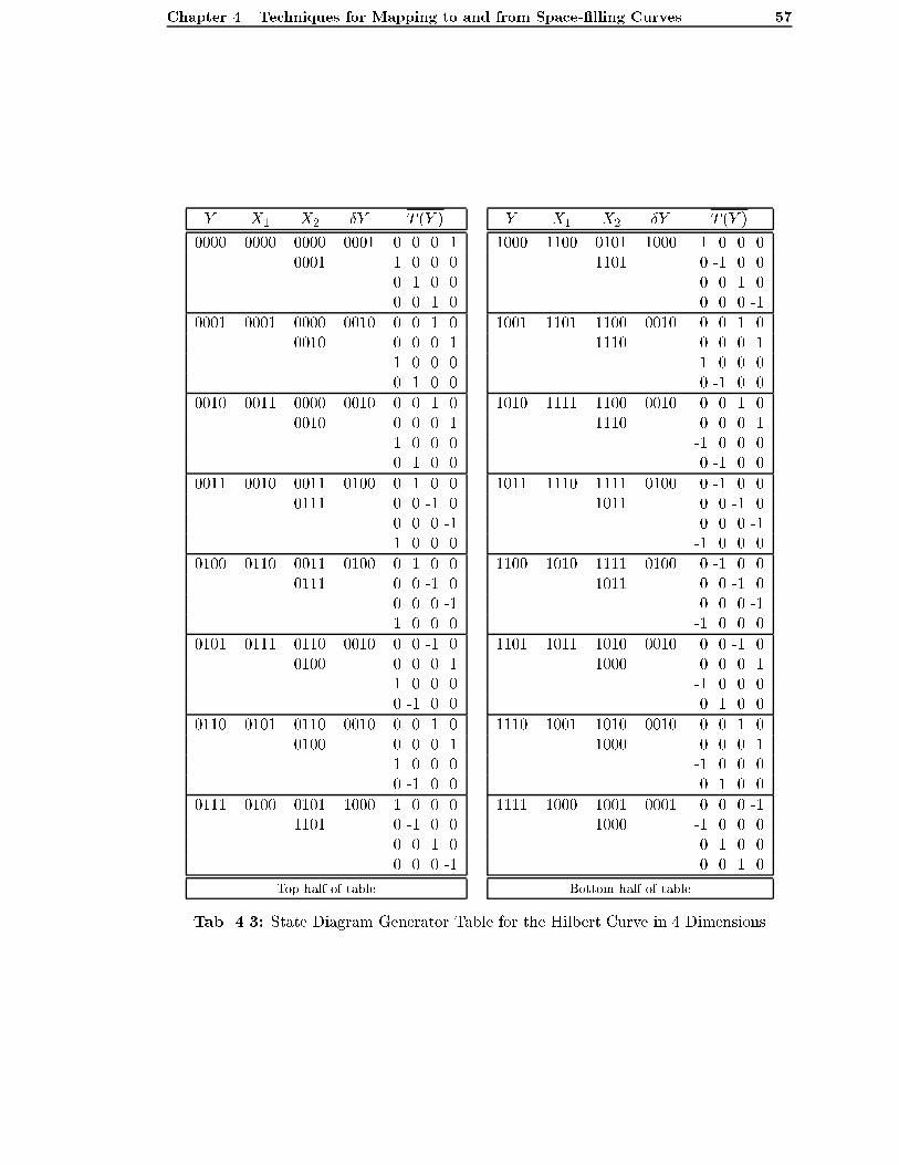
Chapter 4. Techniques for Mapping to and from Space-�lling Curves 57
Y X1 X2 �Y T (Y )
0000 0000 0000 0001 0 0 0 1
0001 1 0 0 0
0 1 0 0
0 0 1 0
0001 0001 0000 0010 0 0 1 0
0010 0 0 0 1
1 0 0 0
0 1 0 0
0010 0011 0000 0010 0 0 1 0
0010 0 0 0 1
1 0 0 0
0 1 0 0
0011 0010 0011 0100 0 1 0 0
0111 0 0 -1 0
0 0 0 -1
1 0 0 0
0100 0110 0011 0100 0 1 0 0
0111 0 0 -1 0
0 0 0 -1
1 0 0 0
0101 0111 0110 0010 0 0 -1 0
0100 0 0 0 1
1 0 0 0
0 -1 0 0
0110 0101 0110 0010 0 0 -1 0
0100 0 0 0 1
1 0 0 0
0 -1 0 0
0111 0100 0101 1000 1 0 0 0
1101 0 -1 0 0
0 0 1 0
0 0 0 -1
Top half of table
Y X1 X2 �Y T (Y )
1000 1100 0101 1000 1 0 0 0
1101 0 -1 0 0
0 0 1 0
0 0 0 -1
1001 1101 1100 0010 0 0 1 0
1110 0 0 0 1
-1 0 0 0
0 -1 0 0
1010 1111 1100 0010 0 0 1 0
1110 0 0 0 1
-1 0 0 0
0 -1 0 0
1011 1110 1111 0100 0 -1 0 0
1011 0 0 -1 0
0 0 0 -1
-1 0 0 0
1100 1010 1111 0100 0 -1 0 0
1011 0 0 -1 0
0 0 0 -1
-1 0 0 0
1101 1011 1010 0010 0 0 -1 0
1000 0 0 0 1
-1 0 0 0
0 1 0 0
1110 1001 1010 0010 0 0 -1 0
1000 0 0 0 1
-1 0 0 0
0 1 0 0
1111 1000 1001 0001 0 0 0 -1
1000 -1 0 0 0
0 1 0 0
0 0 1 0
Bottom half of table
Tab. 4.3: State Diagram Generator Table for the Hilbert Curve in 4 Dimensions

Chapter 4. Techniques for Mapping to and from Space-�lling Curves 58
( 01 )[ 11 ]
State 0
State 1 State 2( 11 )[ 10 ]
( 00 )[ 00 ] [ 01 ]
( 10 )
[ 00 ]
[ 01 ][ 10 ]
[ 11 ]( 11 )
( 00 ) ( 10 )
( 01 )
( 11 )
( 00 ) ( 10 )
( 01 )[ 00 ][ 01 ]
[ 10 ] [ 11 ]
( 11 )
( 00 ) ( 10 )
( 01 )
[ 00 ]
[ 01 ] [ 10 ]
[ 11 ]
[sequence numbers]
(coordinates)
Example:The point with coordinates x = 0 and y = 1 in state 1has a sequence number of3 and its next-state is state 3
State 3
Fig. 4.1: A State Diagram for the Hilbert Curve in 2 Dimensions
binary radix. Bially does not, however, con�ne his interest to spaces where the coordinates
of points are expressed in any particular radix and so he does not apply his technique to
any curve in particular. For example, Bially illustrates the application of his technique
with a generator table for the Peano curve in 2 dimensions (Fig. 2 in [Bia69]) which is
expressed in a ternary radix and the Hilbert curve in 3 dimensions (Fig. 3 in [Bia69])
which is expressed in a binary radix. We note that the latter is a di�erent de�nition of
the curve to that we produce in Figure B.2 in appendix B.
A generator table is comprised of a �xed number of rows and columns. Each row
corresponds to a point lying on a �rst order curve, thus there are rn rows in total, where r
denotes the radix used for representing coordinate values. The rows are ordered according
to the sequence numbers of the points on the curve and together they de�ne the �rst order
curve which corresponds to the �rst state in the diagram.
The table also encapsulates how a transformation of a �rst order curve to a second order
curve is e�ected. We recall from chapter 3 that conceptually this is done by replacing each
point on the �rst order curve with another �rst order curve of some particular orientation,
possibly the same as the original. In the context of a state diagram, these replacement
curves are called next-states. These next-states are de�ned, in part, by transformation
matrices, which are described in more detail below.
The table is populated by following rules which determine the relationships between
various entries within the generator table. These enable the table to be populated manu-
ally but following the rules can be problematic since choices sometimes need to be made
between options which equally satisfy them. Bially does not provide algorithms which
enable the table to be populated in a routine manner, in part because every variation
e�ectively results in the description of a di�erent curve. He notes that some apparently
suitable choices may prevent the process from being completed and, therefore, a certain

Chapter 4. Techniques for Mapping to and from Space-�lling Curves 59
amount of `trial and error' may be required.
The columns in the generator table are headed with the terms Y , X1, X2, �Y and
T (Y ), the meanings of which are given below. It is in the rules for populating columns
X1, X2 and T (Y ) in particular where ambiguities lie.
SUMMARY OF THE RULES
In the remainder of this section, we summarize Bially's rules, providing a commentary
on their signi�cances. We distinguish the rules from the commentary by setting the rules
in a di�erent typeface from that generally used in this thesis and by indenting them.
Column Y
Each row contains a number taken from the integer range
[ 0; : : : ; rn � 1 ]. No number is used twice. The numbers are
arranged in ascending order. Each number contains n digits,
where n is the number of dimensions. Each digit is taken from
the range [ 0; : : : ; r � 1 ].
Column Y holds all of the members of the domain of a mapping from one dimension
to points in n-dimensional space for a �rst order curve. Each value is a distance from the
start of a curve, ie the derived-key, of a point on the curve.
Column X1
Contains the same numbers used in column Y but re-ordered such
that pairs of adjacent entries differ in one digit only and the
difference between different digits is 1. The first entry is 0
and the last entry contains only the digits 0 and (r � 1). The
number of digits of (r � 1) in value is assigned to a variable H
for later reference. Numbers which require less than n digits
are padded on the left with zeros.
Similar to column Y , column X1 holds all of the members of the range of a mapping.
Each member is a point lying on a �rst order curve, expressed as a set of single digit
coordinates concatenated into a single value, ie an n-point as de�ned in chapter 3. The
derived-key, or distance of a point from the �rst point on the curve, is the corresponding
column Y value in the same row. It is because points which are of unit distance apart on
the curve are also adjacent in space that a pair of n-points in adjacent rows in the table
di�er by unit value in one coordinate, ie digit, only.
A value of 0 for the �rst entry in column X1 is equivalent to starting the curve at
the origin of space. This in not, however, necessary. We could, for example, construct
a table for the Hilbert curve as shown in Tables 4.1, 4.2 and 4.3 but with the sequence
of column X1 values reversed from top to bottom in the table. The speci�cation of the
last entry implies that the curve ends at a (di�erent) point on the surface of a hyper-cube
described by a �rst order curve. This follows automatically where a radix of 2 is used. If
a �rst order curve did not begin and end at points on the surface of the hyper-cube, then
it would not be possible to transform it to a continuous second order curve.
Taken together, columns Y and X1 completely describe a mapping to a particular �rst
order curve or state. This state is numbered state S0.
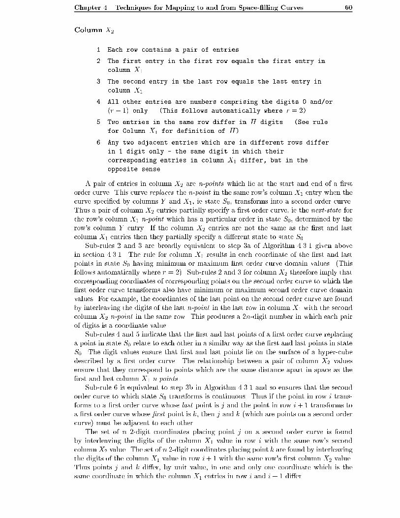
Chapter 4. Techniques for Mapping to and from Space-�lling Curves 60
Column X2
1. Each row contains a pair of entries.
2. The first entry in the first row equals the first entry in
column X1.
3. The second entry in the last row equals the last entry in
column X1.
4. All other entries are numbers comprising the digits 0 and/or
(r � 1) only. (This follows automatically where r = 2).
5. Two entries in the same row differ in H digits. (See rule
for Column X1 for definition of H).
6. Any two adjacent entries which are in different rows differ
in 1 digit only - the same digit in which their
corresponding entries in column X1 differ, but in the
opposite sense.
A pair of entries in column X2 are n-points which lie at the start and end of a �rst
order curve. This curve replaces the n-point in the same row's column X1 entry when the
curve speci�ed by columns Y and X1, ie state S0, transforms into a second order curve.
Thus a pair of column X2 entries partially specify a �rst order curve, ie the next-state for
the row's column X1 n-point which has a particular order in state S0, determined by the
row's column Y entry. If the column X2 entries are not the same as the �rst and last
column X1 entries then they partially specify a di�erent state to state S0.
Sub-rules 2 and 3 are broadly equivalent to step 3a of Algorithm 4.3.1 given above
in section 4.3.1. The rule for column X1 results in each coordinate of the �rst and last
points in state S0 having minimum or maximum �rst order curve domain values. (This
follows automatically where r = 2). Sub-rules 2 and 3 for column X2 therefore imply that
corresponding coordinates of corresponding points on the second order curve to which the
�rst order curve transforms also have minimum or maximum second order curve domain
values. For example, the coordinates of the last point on the second order curve are found
by interleaving the digits of the last n-point in the last row in column X1 with the second
column X2 n-point in the same row. This produces a 2n-digit number in which each pair
of digits is a coordinate value.
Sub-rules 4 and 5 indicate that the �rst and last points of a �rst order curve replacing
a point in state S0 relate to each other in a similar way as the �rst and last points in state
S0. The digit values ensure that �rst and last points lie on the surface of a hyper-cube
described by a �rst order curve. The relationship between a pair of column X2 values
ensure that they correspond to points which are the same distance apart in space as the
�rst and last column X1 n-points.
Sub-rule 6 is equivalent to step 3b in Algorithm 4.3.1 and so ensures that the second
order curve to which state S0 transforms is continuous. Thus if the point in row i trans-
forms to a �rst order curve whose last point is j and the point in row i+ 1 transforms to
a �rst order curve whose �rst point is k, then j and k (which are points on a second order
curve) must be adjacent to each other.
The set of n 2-digit coordinates placing point j on a second order curve is found
by interleaving the digits of the column X1 value in row i with the same row's second
columnX2 value. The set of n 2-digit coordinates placing point k are found by interleaving
the digits of the column X1 value in row i+ 1 with the same row's �rst column X2 value.
Thus points j and k di�er, by unit value, in one and only one coordinate which is the
same coordinate in which the column X1 entries in row i and i+ 1 di�er.

Chapter 4. Techniques for Mapping to and from Space-�lling Curves 61
Column �Y
Each row contains a number such that each digit is the magnitude
of the difference between the corresponding digits in the same
row's 2 entries in column X2. The number will contain H digits
with value (r � 1) and (n�H) digits with the value 0.
This column was implied only in Bially's paper. The �Y values are used in determining
the permutation matrices in the last column of the table. The entry in column �Y for any
row indicates in which dimension(s) the start and end points of the �rst order curve at the
second order level have di�erent coordinate values. A corresponding value for the entries
in the �rst and last rows in column X1 would be equal to the last entry in column X1,
since the �rst entry contains zero-valued digits only.
Column T (Y )
1. Initialize each row's transformation matrix as a permutation
matrix defined such that when the matrix is applied to its
row's �Y value, it produces a value equal to the last entry
in column X1.
2. Adapt the permutation matrix in the following manner: if
the i-th digit of the first of its row's pair of X2 entries
is non-zero then the non-zero element of the i-th column
within the matrix is set to �1.
A transformation matrix encapsulates how a �rst order curve di�ers from the �rst
order curve which is de�ned by columns Y and X1 and which we call state S0. In the
context of the generator table, it encapsulates how a �rst order curve whose �rst and last
point's coordinates (expressed as n-points) are given as a pair of entries in column X2
di�ers from state S0. Thus the matrices imply the next-state for each point in state S0, ie
each point in column X1.
The transformation matrix for state S0 itself is equal to the identity matrix which, if
applied to points in column X1, induces no changes.
Generally, a transformation matrix implies some state Si, Si 6= S0, by enabling any
point Pi in state Si to be transformed into the equivalent point P0 in state S0 which has
the same distance from the beginning of the curve in state S0 as does point Pi in state
Si. The distance, ie sequence number, of point Pi from the start of the curve in state Siis then determined by looking up the column Y value for point P0 in state S0.
It follows that applying a row's matrix to its �rst entry in column X2 should transform
it to the �rst entry in column X1 and applying it to its second entry should transform it
to the last entry in column X1.
In general, more than one transformation matrix satisfying the rules given above can
be constructed for any row and di�erent choices may ultimately result in state diagrams
which contain a di�erent number of states for the same curve.
Concluding Remarks
In general, a state diagram will contain many more states than are encapsulated in
the table. The characteristics of all other states can be determined, however, from the
information contained in it.
An algorithm allowing all states required to produce a state diagram which utilizes the
generator table is given in section 4.3.6.

Chapter 4. Techniques for Mapping to and from Space-�lling Curves 62
We do not describe here how a matrix is used to transform a point or another matrix
but address this also in section 4.3.6.
The rules summarized in the previous section do not guarantee that a state diagram
can be successfully generated and nor do they guarantee that a state diagram containing
the minimum possible number of states can be generated. This is discussed further in
Bially's PhD thesis [Bia67].
4.3.3 State Diagram Generator Table for the Hilbert Curve
In the context of Bially's state diagram generation technique, the Hilbert curve is the
special case of a space-�lling curve for which coordinates and derived-keys are expressed
using a binary radix.
In this section, we present specialized algorithms which extend Bially's rules for pop-
ulating columns X1, X2 and T (Y ) of the generator table. These are used in conjunction
with the rules for columns Y and �Y described above. Together, they enable a generator
table for an arbitrary variant of the Hilbert curve to be constructed for any number of
dimensions.
The precise form of the arbitrary variant is dictated by the detail of our rules. For
example, the rules for columns Y and X1 determine the orientation and direction of
traversal of the �rst order approximation of the curve. The rules for each of columns X1,
X2 and T (Y ) may be modi�ed to produce alternative variants of the curve and we discuss
this further in section 4.3.4.
In Figure 4.2 we give an example of the second order 3-dimensional Hilbert curve
implied by the generator table given in Table 4.2 which was constructed in accordance
with the rules described in this section.
Once implemented, the rules enable the table to be constructed automatically. This
is desirable since populating the tables manually becomes increasingly time consuming as
the number of dimensions in a space rises.
The task of developing algorithms for the generator table is facilitated by identifying
and ensuring that we preserve in higher dimensions two characteristics of the 2-dimensional
Hilbert curve.
The �rst of these is a symmetry about a line which is the normal to one of the axes.
The corollary of this is that all of the points lying on one half of the curve have the value
of zero for their coordinates in one dimension and all of the others have the value of one
for their coordinates in the same dimension. In higher than 2 dimensions, curves need not
be symmetrical, as illustrated in Figure 3.5(c) in chapter 3, but we con�ne our interest to
those which are since they are more readily described in a state diagram generator table.
The second characteristic is that the �rst and last points of a �rst order approximation
are adjacent. In higher than 2 dimensions it is possible to construct �rst order curves which
do not have this characteristic, as illustrated in Figure 3.7 in chapter 3. In 3 dimensions at
least we are unable to utilize them to produce higher order curves which are continuous.
In the remainder of this section we set out our rules for populating the generator table
for the Hilbert curve. In doing so, we provide a commentary on their signi�cances. We
use the term bit where the term digit was used in the summary of Bially's rules in the
previous section, since the Hilbert curve is represented using a binary radix.
Column Y
As described in section 4.3.2.

Chapter 4. Techniques for Mapping to and from Space-�lling Curves 63
Fig. 4.2: Second Order 3-dimensional Hilbert Curve Implied by our State Diagram Gen-
erator Table in Table 4.2

Chapter 4. Techniques for Mapping to and from Space-�lling Curves 64
Column X1
Column X1 expresses the ordering of points on a �rst order curve. The characteristics
identi�ed above together with those required by Bially's generic rules are conveniently
found to be shared by the Gray-code sequence of numbers described in chapter 3. Thus
the rule for column X1 may be stated as follows:
Calculate each column X1 entry as Y � Y=2, as described in
[RND77]1.
A member of a Gray-code sequence of order n can be considered as the set of co-
ordinates of a point on a �rst order curve in n dimensions where the coordinates have
been concatenated into a single value, ie expressed as an n-point. A complete sequence of
Gray-codes of order n is then equivalent to the set of points on a �rst order curve ordered
such that adjacent points in the sequence are adjacent in space; that is, they di�er in one
coordinate (or bit in an n-point) only.
Populating column X1 with the Gray-code sequence thus ensures that the �rst entry
has the value of zero in all bits and that the last entry has the value of one in one bit only.
The Gray-code sequence dictates that this is the top bit. We label this bit position P for
reference later on. Use of the Gray-code sequence results in the �rst and last entries being
adjacent points in space and the value of the variable H, de�ned by Bially in his rule for
column X1 , becomes one. The symmetry of the Hilbert curve is also achieved since the
�rst half of the values have a zero in bit position P and the second half have a value of
one and, in other bits, the values in row i equal the values in row 2n � 1� i. Bit position
P indicates the axis in n-dimensional space which the start and end of the curve of any
order lie on.
The use of Gray-codes was suggested by Faloutsos [FR89b] without explanation.
Column X2
In populating column X2, one method of specializing Bially's rules for the Hilbert
curve proceeds as follows:
In the �rst row, the �rst entry is set to 0 and the second is set to equal the X1 value
found in the second row.
For each row, from the second to the last in the �rst half of the table, we copy the
second entry from the previous row into the �rst entry in the current row and adjust it
according to Bially's sub-rule 6 for column X2. We then copy the �rst entry from the
current row into the second entry of the current row and again adjust the second entry
according to sub-rule 6.
As with column X1, all of the entries, taken individually, in the second half of the table
are a re ection of those in the �rst half, except in the bit in position P . All of the entries
in the �rst half will have bits in position P set to 0 except for the last entry where it will
equal 1 and all of the entries in the second half will have bits in position P set to 1 except
for the �rst entry where it will equal 0.
In 2 and 3 dimensions, the above procedure enables the column to be populated auto-
matically. A problem occurs in higher dimensions, however, in that sometimes a pair of
entries in the same row may have the same value.
This problem needs to be resolved by changing the value of one of the bits in the second
entry. This change must result in no entry in the column being equal to its corresponding
entry in column X1 (except for the �rst and last entries which must equal their X1 values).
Any bit may be chosen arbitrarily, provided it is not the bit in position P or the bit whose
value is determined by Bially's sub-rule 6 for column X2.
1 Refer to appendix A for a key to symbols.

Chapter 4. Techniques for Mapping to and from Space-�lling Curves 65
A pattern emerges from an examination of the column X2 entries produced in the
above manner for 2 and 3-dimensional curves which can be expressed as an algorithm
enabling the column to be automatically generated in higher dimensions. The algorithm
is similar to that which generates the Gray-code sequence. We call its output the X2Gray-
code sequence and its construction can be illustrated with the following examples:
Order 1: [ 0; 1; 0; 1 ]2
Order 2: [ 00; 01; 00; 10; 00; 10; 11; 10 ]
Order 3: [ 000; 001; 000; 010; 000; 010; 011; 111; 011; 111; 110; 100; 110; 100; 101; 100 ]
Our rules which generate the sequences is given as follows:
1. Initialize a sequence of order 1 as: [ 0; 1; 0; 1 ]. Individual
members of this sequence are identified by labels as
follows: [ a; b; c; d ].
2. The order 2 sequence is derived from the order 1 sequence in
a number of steps as follows:
(a) Initialize the sequence as the order 1 sequence followed
by the reverse of the order 1 sequence thus:
[ a; b; c; d; d; c; b; a ].
(b) Replace the fourth value with the third value and the
fifth value with the sixth value thus:
[ a; b; c; c; c; c; b; a ].
(c) Prefix members of the first half of the sequence with a
bit of value zero and the members of the second half
with a bit of value one thus: [ 0a; 0b; 0c; 0c; 1c; 1c; 1b; 1a ].
(d) Invert the values of the top bits of the fourth and
fifth members of the sequence thus:
[ 0a; 0b; 0c; 1c; 0c; 1c; 1b; 1a ]. This produces the following
sequence of binary numbers: [ 00; 01; 00; 10; 00; 10; 11; 10 ].
This is the sequence of order 2.
3. Generally, given a sequence of order j as:
[ a0; a1; : : : ; a2j+1�2; a2j+1�1 ], where each ai is a binary value,
the sequence of order j + 1 is defined as:
[ 0a0; 0a1; : : : ; 0a2j+1�2; 1a2j+1�2; 0a2j+1�2; 1a2j+1�2; : : : ; 1a2j+1�1 ].
Thus the sequence of entries for rows in column X2 for a curve in n dimensions can be
populated with an X2Gray-code sequence of order n. Each pair of values corresponds to
the �rst and last coordinates of points on a �rst order curve to which a point taken from
column X1 transforms to at the second order level.
2 NB: usage of the term order here is distinct from usage in the context of order of curve

Chapter 4. Techniques for Mapping to and from Space-�lling Curves 66
Alternatively, the algorithm can be stated more simply in the following terms, where
we derive a column X2 sequence for a curve of n dimensions from the sequence for n� 1
dimensions, initializing the sequence for 1 dimension as [ 0; 1; 0; 1 ].
1. Initialize the sequence for Order n equal to the sequence
for order n� 1.
2. Set the value of the last member of the sequence (for order
n� 1) equal to the value of the penultimate member.
3. Prefix the last member of the sequence with a bit of value 1
and all other members each with a bit of value 0.
4. Double the size of the sequence by reflecting it such that
the last member equals the first and so on.
5. Invert the values of the most significant bits of all of the
members in the second half of the sequence.
In experiments, the application of both of the above procedures has enabled us to
produce correct results but a proof of correctness for them needs to be formulated.
Column �Y
As described in section 4.3.2.
For the Hilbert curve, any row's �Y value contains only one bit set to one and all other
bits set to zero. (This is consistent with the variable H referred to above having a value
of one). The bit which is set to one denotes the axis on which lie the �rst and last points
of the �rst order curve, partially encapsulated by entries in column X2, to which a point
in column X1 transforms to at the second order level.
A single non-zero digit within a �Y value implies that a pair of columnX2 entries lie on
the same edge of a hyper-cube described by the line connecting the points lying on a �rst
order curve. This is consistent with the observation made in section 4.2 above where we
consider the number of di�erent types of node which can exist in the tree representation
of the Hilbert curve.
Column T (Y )
The transformation matrices for the Hilbert curve may be calculated in a more straight-
forward manner than that described in the generic procedure. This arises from column �Y
values containing a single non-zero bit only. We label the bit positions in �Y : 1; 2; 3; : : : ; n;
where bit position 1 corresponds to the most signi�cant bit and bit position n corresponds
to the least signi�cant bit.
For each row:
1. Initialize the matrix to the identity matrix.
2. Create a permutation matrix by interchanging the first row
of the matrix with the j-th row, where j designates the
position of the single non-zero bit in the row's �Y value.
3. Determine the signs of the non-zero elements of the
permutation matrix in accordance with Bially's rule given in
the previous section, thus creating a transformation matrix.

Chapter 4. Techniques for Mapping to and from Space-�lling Curves 67
It follows from these rules that if a column �Y value is 10 : : : 0, then the permutation
matrix produced in step 3 is the identity matrix.
We discuss state diagram growth rates, as the number of dimensions in a space in-
creases, below in section 4.3.7. Equations (4.7) and (4.8) given in that section express
lower and upper bounds on the number of states which result from application of the gen-
erator table. We note here, however, that the rules given above result in the production
of valid state diagrams containing a number of states equal to the upper bound. Clearly,
it is desirable if state diagrams are as compact as possible since they occupy memory.
We are able to achieve the lower bound on state diagram size by modifying our method
of setting up the permutation matrices in sub-rules 1 and 2. In doing this, it is convenient
to represent each row in a matrix as an n-bit value, ie where all of a row's column entries
are concatenated into a single value. Thus the sub-rules are replaced by the following:
1. Set the first row of a matrix equal to its corresponding
column �Y value.
2. For each row, numbered 2 : : : n, in the matrix, set row i equal
to the value in row i� 1, circular right-shifted one bit
position.
In the remainder of this thesis, we adopt this approach for the de�nition of transfor-
mation matrices where we use state diagrams.
4.3.4 Variations to State Diagram Generator Tables for the Hilbert
Curve
We note in chapter 3 that the Hilbert curve is a concept which may be expressed in
di�erent ways. We also recall that our rules for the Hilbert curve state diagram generator
table enable the production of a state diagram for an arbitrary variant of the curve. In
this section, we brie y discuss some of the ways in which our rules may be altered in order
to produce di�erent variations.
In presenting our rules for column X1 in the previous section, we labelled the top bit
position P . The values in the rows in the top half of the table all have the value zero in
this position and those in the bottom half all have the value one in this position. Having
constructed the table in the manner described, we can de�ne an alternative orientation of
the curve as a whole. This is done by interchanging the values of the bit in position P
with the value of the bit in some other position j in all entries in all columns except in
column Y .
We noted in section 4.3.2 that our state diagram given in Figure B.2 in appendix B
for the 3-dimensional Hilbert curve di�ers from that given in Fig. 3 of [Bia69]. Clearly,
this implies that Bially populated column X2 of the generator table in a di�erent manner
to that adopted by ourselves.
We saw in the previous section that there are alternative ways of initializing the per-
mutation matrices during the process of de�ning transformation matrices. The second
alternative may be simply varied by performing circular left-shift operations instead of
circular right-shift operations in de�ning the individual rows of the matrices.
In concluding this section, we note that the number of possible variations of the Hilbert
curve increases as the number of dimensions rises and many variants can be encapsulated
by state diagram generator tables. Some of these will result in state diagrams which
contain a larger number of states than others.
In the context of an implementation of an indexing application, one form of the Hilbert
curve is likely to be as suitable as any other, except that it is desirable to choose one where
the state diagram is as compact as possible.

Chapter 4. Techniques for Mapping to and from Space-�lling Curves 68
4.3.5 State Diagram Generator Tables for Discontinuous Curves
Our motivation for carrying out research into the Hilbert curve arises, in part, from an
assumption that it is desirable to base our application on a continuous curve. The results
of preliminary tests carried out and reported on in chapter 10 appear to support this
assumption.
State diagram sizes are discussed in more detail in section 4.3.7 below but for the time
being it is su�cient to note that their growth rate for continuous curves is exponential in
the number of dimensions. According to equation (4.7) in that section, state diagrams for
the Hilbert curve contain at least n 2n�1 states.
According to Bially's equations (4.4) and (4.5), a lower minimum requirement of 2n�1
states applies for space-�lling curves in which the di�erence between all pairs of coordinates
of the �rst and last points of a �rst order curve equals their radix minus one. When this
occurs, the variable H, de�ned in Bially's rule for column X1, given in section 4.3.2,
equals the number of dimensions, ie n. Nevertheless, this still represents an exponential
growth rate. Furthermore, in experiments in 2 and 3 dimensions, we are only able to draw
continuous curves, where H equals n, if coordinates are expressed in an odd numbered
radix. Thus Peano's curve can be represented by a state diagram with only 2n�1 states
but Hilbert's cannot.
Given the exponential growth rates of state diagrams for continuous curves we are
motivated in this section to consider utilization of discontinuous curves as a compromise
for application in higher dimensions. A number of discontinuous curves may be expressed
more compactly with fewer states than continuous curves such as those of Hilbert and
Peano.
4.3.5.1 The Z-order Curve
The Z-order curve [Mor66] can be represented by a state diagram which contains a single
state only. Every point on a curve of order k transforms to the same �rst order curve at
order k + 1. This is apparent from Figures 3.10 and 3.12 in chapter 3. Nevertheless, the
simplicity with which mappings to the Z-order curve are performed renders the application
of state diagrams super uous. Indeed, the mapping between coordinates, expressed as n-
points, in the Z-order curve's single state and sequence numbers is encapsulated by the
identity function.
We recall from chapter 3, however, that the Z-order curve manifests a considerable
number of discontinuities. Pairs of points are adjacent, ie unit distance apart, but the
second point of any pair is never adjacent to the �rst point of the successor pair. Thus the
number of discontinuities within an approximation is given by (2nk=2) � 1 or 2nk�1 � 1.
The magnitude of discontinuities needs to be considered in conjunction with their
frequency when assessing the relative merits of di�erent discontinuous curves. Although
discontinuities occur frequently in the Z-order curve, most are small in magnitude and
therefore should have little adverse e�ect on clustering. Nevertheless, the frequency of
discontinuities motivates us to consider alternative less discontinuous curves.
4.3.5.2 Moore's Curve
The curve which we describe in this section is our discontinuous variation of Moore's
continuous variation of the Hilbert curve [Moo00, Sag94]. Although Moore's curve requires
the same number of states as the Hilbert curve, our variation requires fewer. Compared
with the single state curves the discontinuities found in our variation are fewer in number
and more localized in their extent. We illustrate �rst to fourth order approximations of

Chapter 4. Techniques for Mapping to and from Space-�lling Curves 69
First Order
Third Order
Second Order
Fourth Order
Third Order
Fourth Order
(a) (b)
Fig. 4.3: Approximations of Moore's Curve in 2 Dimensions and our Variations at the
Third and Fourth Orders
Moore's curve in 2 dimensions in Figure 4.3(a). Discontinuities are introduced in our
variation in curves of orders 3 and above and this is shown in Figure 4.3(b).
In 2 dimensions, Moore's �rst order curve has the same form as Hilbert's but the
transformation to a second order curve entails a di�erent set of rotations and re ections.
The transformation to any higher order k, where k > 2, entails replacing each �rst order
curve within the curve of order k with Hilbert's curve of order 2, suitably rotated and/or
re ected, rather than replacing each point with a �rst order curve. The result is a contin-
uous curve but it is not self-similar at every level as the form of the second order curve is
not reproduced in any other order.
Our variation on this curve, replaces every �rst order curve within a curve of order k,
where k > 2, with the curve of order 2. The resulting curve is not continuous in orders
greater than 2 but it is self-similar.
An interesting feature of the curve is that in orders higher than 2, the start and end
points do not lie on any surface of the space through which it traverses.
The procedure for creating the state diagram generator table is the same as for the
Hilbert curve except in columns X2 and T (Y ). Examples of generator tables for 2 { 4
dimensions are given in Tables C.1, C.2 and Table C.3 in Appendix C.
Column X2
As with the Hilbert curve, after manually populating columnX2 in 2 and 3 dimensions,
we are able to identify a pattern which can be expressed as an algorithm, again similar to
that for the Gray-code sequence. We call this the MX2Gray-code sequence. The pattern

Chapter 4. Techniques for Mapping to and from Space-�lling Curves 70
is illustrated with the following examples:
Order 1: [ 0; 1; 0; 1 ]3
Order 2: [ 10; 11; 10; 11; 01; 00; 01; 00 ]
Order 3: [ 110; 111; 110; 111; 101; 100; 101; 100; 000; 001; 000; 001; 011; 010; 011; 010 ]
Our rules which generate the sequences for order n are given as follows:
1. Append a reflection of the sequence for order n� 1 to the
sequence for order n� 1, thus doubling its size.
2. Prefix each member of the first half of the enlarged
sequence with a bit of value one.
3. Prefix each member of the second half of the enlarged
sequence with a bit of value zero.
Thus the sequence of entries for rows in column X2 for a curve in n dimensions can be
populated with an MX2Gray-code sequence of order n. Each pair of values corresponds to
the �rst and last coordinates of points on a �rst order curve to which a point taken from
column X1 transforms to at the second order level.
Column T (Y )
The permutation matrices used in column T (Y ) are set up by exchanging the �rst row
of the identity matrix with one (or no) other, in the manner initially considered for the
Hilbert curve.
We recall that this approach fails to produce state diagrams for the Hilbert curve which
are as compact as possible and that we resolve this by modifying our rules, employing
circular-shifting. In the case of our variation to Moore's curve, the comparative e�ect of
these two methods of de�ning the matrices, in terms of state diagram size, is the reverse
of that which obtains for the Hilbert curve.
4.3.5.3 The Gray-code Curves
We identify three of a number of possible curves which use Gray-codes in section 3.7.2 of
chapter 3 and they are referred to as Gray-codeF , Gray-codeA and Gray-codeB .
We saw in chapter 3 that Gray-code curve mappings rely on mappings between Gray-
codes and their sequence numbers. These are relatively simple and are described in chap-
ter 5. Alternatively, Bially's state diagram approach can be adapted and applied to
performing mappings to the various Gray-code curves. A detailed description of how this
is done is given in appendix D.
4.3.6 Production of State Diagrams from Generator Tables
The information contained within the generator table is su�cient to enable all and only
the states required in a state diagram to be calculated and for the relationships between
those states to be determined.
The method by which a state diagram generator table is used to produce a state dia-
gram is not detailed in Bially's paper [Bia69] although it is addressed from a mathematical
perspective in his PhD thesis [Bia67]. In this section we present an algorithm for gener-
ation of the state diagram in terms which more readily enable it to be implemented as a
3 NB: usage of the term order here is distinct from usage in the context of order of curve

Chapter 4. Techniques for Mapping to and from Space-�lling Curves 71
computer program. The method is independent of the particular curve which is encapsu-
lated by the table. The number of states contained in the resulting state diagram depends
on the detail of the curve as set out in the generator table and not on the way the table
is manipulated.
The generator table is used to produce a temporary list of all of the states which
together de�ne a state diagram. Once created, not all of the information within it is
needed in the �nal state diagram. The list is therefore traversed to extract relevant
information only.
We follow the algorithm with details and examples of how calculations which use trans-
formation matrices are carried out. This section is concluded with an example showing
how part of a state diagram for the Hilbert curve in 2 dimensions is constructed.
The Algorithm
The �rst state placed in the temporary list is the state encapsulated by the generator
table itself; by the mapping de�ned by columns Y and X1 and by the next-states for each
point as de�ned by transformation matrices in column T (Y ).
There is no relationship between consecutive states within the list of states. They are
simply placed in it in the order that they are encountered in the calculation process.
A member of the temporary list de�nes a state and is a record containing the following
information:
1. A state number, u, identifying the state.
2. A set of rn triples, one for each point on a �rst order curve. Each triple is of the
form: hY iu ; X1iu; tm
iu i. Y
iu is a sequence number, in the range [ 0; : : : ; rn � 1 ], of
a point in state number u. X1iu is the n-point representation of the coordinates of
the point, in the same range. tmiu is the number of the next-state, ie �rst order
curve, to which the point transforms to in a second order curve. Each distinct tmiu
number corresponds to a transformation matrix, examples of which are found in
column T (Y ) of the generator table, de�ning a distinct state.
3. A Transformation Matrix. This encapsulates how this state di�ers from the �rst
state in the list. When the matrix is applied to a point, it is transformed into the
equivalent point in the �rst state in the list which has the same sequence number as
the point in this state.
4. A pointer to the next member in the list.
The procedure for building the temporary list of states is given in Algorithm 4.3.2.
In e�ect, this algorithm constructs a tree representation of a space-�lling curve in a
depth-�rst manner. As new nodes are de�ned, they are appended to a list. No node is
added if a node of the same type already exists in the tree (ie, list) and so the tree is not
balanced.
A state diagram, derived from the temporary list of states, can be implemented as
an array of states with one element for each state in the list. A state is identi�ed by its
number, which can be implied by its position within the array of states, and de�ned by
its list of triples. Each list of triples can also be stored as an array. The elements of these
arrays may be expressed compactly as pairs since one of the attributes, Y iu or X1iu, of a
triple can be implied by its position in the array, depending on how the triples are sorted.
Thus two state diagrams can be produced from the state list. One is required for
performing a mapping from one dimension to n dimensions. The triples within it are
sorted by Yiu values, which may be implied. An example for the 2-dimensional Hilbert
curve is given in Table B.2 in appendix B. The other is required for performing a mapping

Chapter 4. Techniques for Mapping to and from Space-�lling Curves 72
Algorithm 4.3.2 Algorithm to Create a List of States
fUsing the generator table, initialize the �rst member, ie state, of the listg
1: current state ( 0
2: next state num ( 1
3: for all i such that 0 � i < rn do
4: Yi0 ( i
5: X1i0 ( X1 value from row i of the generator table
6: end for
fThe tmi0 attributes of the triples are initially unde�nedg
7: current state transformation matrix ( the identity matrix
fInitialize the tmi0 attributes, ie next-state numbers, of the triples in state 0g
8: for all i such that 0 � i < rn do
9: if no state exists in the state list whose transformation matrix equals that found in
row i of the generator table then
10: append a new state to the list
11: new state's number ( next state num
12: next state num ( next state num + 1
13: new state's transformation matrix ( matrix from row i of the generator table
14: tmi0 ( new state's number
15: else
16: tmi0 ( the number of the state found in the list
17: end if
18: end for
fState 0 is now fully de�ned. A new state has been added to the list for each distinct
transformation matrix, other than the identity matrix, found in column T (Y ) of the
generator tableg
fInitialize the attributes of the triples in all of the states remaining in the list, ap-
pending any new states required in the processg
19: for all states, u, in the list (excluding state 0) do
20: for all i such that 0 � i < rn do
21: Yiu ( i
22: end for
23: for all i such that 0 � i < rn do
24: j ( i � the transformation matrix for state u
25: p( the row in state 0 such that X1p0 = j
26: X1pu <= i
fie assign i to the X1 value in row p of the current state ug
27: TM ( (transformation matrix corresponding to tm
p0) � (transformation matrix
corresponding to state u)
fNB TM is a transformation matrix de�ning a state, not a state numberg
28: if no state exists in the state list whose transformation matrix equals TM then
29: Add a new state to the list
30: State Number of the new state ( next unused number
31: Transformation matrix of the new state ( TM
32: end if
33: tmpu ( the State Number of the state whose transformation matrix equals TM
34: end for
35: end for

Chapter 4. Techniques for Mapping to and from Space-�lling Curves 73
from n dimensions to one dimension. The triples are sorted by X1iu values, which may be
implied. An example for the 2-dimensional Hilbert curve is given in Table B.3. Both of
these examples are produced from the generator table given in Table 4.1 and de�ne the
state diagram illustrated in Figure 4.1.
Similarly, Tables B.4 and B.5 in the appendix correspond to the 3-dimensional Hilbert
curve and are derived from the generator table given in Table 4.2 and de�ne the state
diagram illustrated in Figure B.2. Tables B.6 and B.7 correspond to the 4-dimensional
Hilbert curve and are derived from the generator table given in Table 4.3.
Transformation Matrix Operations
Two di�erent transformation matrix calculations are employed in Algorithm 4.3.2;
in line numbers 24 and 27. We conclude this section with a description of how these
calculations are performed.
In our description, matrix rows are numbered in the range [ 1; : : : ; n ] from top to
bottom and columns are numbered in the same range from left to right. A state is referred
to as `Su', where `u' is the state number. State S0 is the state which is encapsulated by
the generator table itself.
We de�ne P eu as the column Y value corresponding to the column X1 value equal to
e, in state Su. e is expressed as a binary number and u is expressed as a decimal number.
Determining the value of P eu is achieved with the aid of the calculation performed in
line 24 of Algorithm 4.3.2. e is multiplied by the transformation matrix for state Su in
order to determine the equivalent column X1 value, f , in state S0 which maps to the same
column Y value. Thus P eu = P
f0 .
The multiplication is carried out in the following manner, using a temporary variable
V which is an n-bit vector:
1. V is initialized such that column i contains a non-zero value if the non-zero value
in the same column in the transformation matrix for state Su is negative, for all
1 � i � n. Thus V encapsulates the signs of the non-zero elements of the matrix for
state Su.
2. f is initialized as e � V .
3. For each row i in the matrix for Su, if a non-zero value exists in column j of row i
and a non-zero value exists in the same column in f , then the non-zero value in
column j of f is moved to column i in f .
4. P eu is assigned the value of P
f0 , found by looking up the column Y value corresponding
to the column X1 of f in the generator table.
The order in which the above operations is performed is signi�cant.
Having found the column Y value for e, we need also determine its next-state. This is
achieved with the aid of the calculation performed in line 27 of Algorithm 4.3.2. The next-
state transformation matrix (A) for e is de�ned as the next-state transformation matrix
for f in state S0 (B) multiplied by the transformation matrix for state Su (C). More
succinctly, A ( B � C.
The multiplication is carried out by examining each row of matrix B in turn:
1. If in row i of matrix B, a non-zero bit exists in column j, then row i of matrix A
takes the value of row j of matrix C.
2. If the signs of the non-zero values in row i of matrix B and row j of matrix C are
di�erent, ie one is positive and one is negative, then the sign of the non-zero value
in row i of matrix A becomes negative, otherwise it becomes positive.

Chapter 4. Techniques for Mapping to and from Space-�lling Curves 74
The matrix multiplication is not commutative.
Figure 4.4 gives an example of the transformation matrix calculations described in
this section when applied to the 3-dimensional Hilbert curve de�ned in Table 4.2 and
illustrated in Figure B.2. The example shows how the column X1 value of `010' in state
number `11' (decimal) maps to the column Y value of `111' and that it's next-state is state
number `2'. This is consistent with Figure B.2.
An Example
Figure 4.5 illustrates part of the process of constructing a list of states for the Hilbert
curve in 2 dimensions.
4.3.7 State Diagram Growth Rate
Having described and developed the state diagram approach to mapping between one
dimension and n dimensions for a number of space-�lling curves, in this section we compare
them from the point of view of state diagram size.
4.3.7.1 The Hilbert Curve
Bially observed that it is possible to limit the number of states in a state diagram for a
continuous space-�lling curve to the smaller of those given by
n !
(n�H) !2n�
12(1�(�1)H ) (4.4)
andn !
H !2n�
12(1�(�1)H ) (4.5)
An upper limit on the number of states required is given by
n ! 2n�12(1�(�1)H ) (4.6)
In the case of the Hilbert curve, where H = 1, we can replace equation (4.4) with
n 2n�1 (4.7)
and replace equations (4.5) and (4.6) with
n ! 2n�1 (4.8)
We note that equation (4.7) is the same as equation (4.3) from section 4.2 above, which
gives the number of edges in a hyper-cube.
The number of states produced by our technique for the Hilbert curve, described in
section 4.3.3, conforms with (4.7) or (4.8), depending on how the transformation matrices
are initialized. Were we to interchange the �rst row of an identity matrix with one other,
the latter would apply. Where the �rst row of a matrix is initialized to its row's column �Y
value and successive rows are determined by circular shifting, the former applies.
In accordance with equation (4.7), the rate at which the number of states in a diagram
increases is exponential in the number of dimensions. This limits the number of dimensions
in which mappings may be performed with the aid of state diagrams in the implementation
of our indexing application. The rate of increase in the size of an individual state is also
exponential in the number of dimensions. The size of a state is proportional to the number
of points on a �rst order curve.
Table 4.4 contains a summary of the number of states required for the Hilbert curve,
and others discussed in this chapter, as the number of dimensions varies. Considering the

Chapter 4. Techniques for Mapping to and from Space-�lling Curves 75
Example for: state u = 11 (decimal)
e = 010 (binary)
(e is a column X1 value)
Matrix for state 11 (decimal) is
shown in the state diagram of Fig-
ure B.2 in appendix B. This matrix
is referred to as `matrix C' below.
Find the column Y value, P e
u, for e
Step 1: V ( 011 (since 1's in last 2 columns of matrix C are negative)
Step 2: f ( 010� 011 (ie f ( e� V , therefore, f = 001)
Step 3: The 1 in column 3 of row 1 in matrix C causes the 1 in column 3 of f to move
to column 1.
Thus f ( 100
Other rows in matrix C have no e�ect since 1's in their columns all correspond
to 0's in the same columns in f .
Step 4: From generator table (Table 4.2 { encapsulating state 0), Pf
0= 111
Therefore, P e
u( 111
Find the next-state for e
next-state for f (= 100) in state 0 is state 4 (matrix B) { from generator table.
Step 1: apply matrix B to matrix C to create matrix A
0 0 -1 (1) 0 0 -1 (4) 0 -1 0 (7)
-1 0 0 (2) � 1 0 0 (5) ! 0 0 -1 (8)
0 1 0 (3) 0 -1 0 (6) 1 0 0 (9)
B C A
(1) causes (6) to move to (7),
(2) causes (4) to move to (8),
(3) causes (5) to move to (9).
Step 2: adjust signs of non-zero elements in matrix A
signs in (1) and (6) are both negative, therefore sign in (7) becomes positive,
signs in (2) and (4) are both negative, therefore sign in (8) becomes positive,
signs in (3) and (5) are both positive, therefore sign in (9) becomes positive.
Thus matrixA (
0 1 0
0 0 1
1 0 0
From the state diagram in Fig-
ure B.2, matrix A corresponds to
state 2
Therefore, next-state for e( state 2.
Fig. 4.4: Example Showing Calculations Carried Out Using Transformation Matrices

Chapter 4. Techniques for Mapping to and from Space-�lling Curves 76
01
11
0
0
2
1
10
0
1
1
0
1
0
0
1
00
01
10
11
1
1
3
0
1
0
0
1
1
0
0
1
1
0 1
0
0
0
1
1 0 0 1
0 1 1 0X
0-1 0 1
-1 0 1 0X
1 0 0 1
0 1 1 0X
0 1 0 1
1 0 1 0X
0 1
1 0 0 1
1 0 0-1
-1 0 0 1
1 0= = ==
* **
1
X1 tm
State 2
Y
0 -1
0-1
Y
00
X1 tm
State 0
After execution of After execution oflines 1 - 7
X1 tm
State 1
Y
loop in lines 8 - 18NB: Line numbers
Algorithm 4.3.2relate to
NB: At this stage, only those states referred to in thegenerator table appear in the list, ie states 0, 1 & 2.
Iteration 4Iteration 3Iteration 2Iteration 1
00
00 10
10
01
11
11
00 11 01 10
00
01
10
11
00 00 00
01 01
10
0 0
1
3
0
3
X1 tm
State 1
Y
00
01
10
11
X1 tm
State 1
Y
00
01
10
11
X1 tm
State 1
Y
00
01
10
11
X1 tm
State 1
Y
00
01
10
11
j
p
01i
(line 25)
(line 33)
(line 24)
(line 27)
TM
tm 0 3 1 1
now added to state list
Loop in lines 20 - 22 populates column Y
(iterations for state numbers 2 and 3 carried out in a similar manner)
Loop in lines 23 - 34:
First iteration of loop in lines 19 - 35; ie for State 1
new state (no. 3) is
**
*
X1pu tm
p0
Fig. 4.5: An Example of the State Diagram Generation Process

Chapter 4. Techniques for Mapping to and from Space-�lling Curves 77
No. Hilbert Moore Gray-codeF Gray-codeA;B
of
dims No. of size No. of size No. of size No. of size
states (kB) states (kB) states (kB) states (kB)
3 12 0.1875 8 0.125 4 0.0625 2 0.03125
4 32 1 16 0.5 8 0.25 2 0.0625
5 80 5 32 2 16 1 2 0.125
6 192 24 64 8 32 4 2 0.25
7 448 168 128 32 64 16 2 0.5
8 1024 768 256 128 128 64 2 1
9 2304 4608 512 1024 256 384 2 3
10 5120 20480 1024 4096 512 2048 2 6
11 11264 90112 2048 16384 1024 8192 2 12
12 24576 393216 4096 65536 2048 32768 2 24
13 53248 1703936 8192 262144 4096 131072 2 48
14 114688 11010048 16384 1048576 8192 524288 2 96
15 245760 47185920 32768 4194304 16384 2097152 2 192
16 524288 201326592 65536 16777216 32768 8388608 2 384
Tab. 4.4: State Diagram Generator Table Growth Rates and Memory Requirements
growth rates of both state diagrams and individual states the table also summarizes the
amount of memory required to store state diagrams. It appears that a practical upper
limit of 8 or 9 dimensions applies to the Hilbert curve. It appears that above 8 or 9
dimensions state diagram storage requirements for the Hilbert curve become prohibitive.
The stepped horizontal line in the table notionally indicates the numbers of dimensions for
di�erent curves beyond which it becomes impracticable to store state diagrams in memory,
given current hardware constraints.
When evaluating the cost of utilizing state diagrams, factors other than their sizes
need also to be taken into account.
As the size of a state diagram increases with the increase in the value of n, so also does
the time taken to load the diagram into memory. However an application using a state
diagram needs only to load it once each time it is executed.
From a practical view, it is also advantageous to maintain two copies of the state
diagram in memory since some operations entail mapping from one dimension to n dimen-
sions while others entail the inverse. Clearly this doubles the memory requirements listed
in Table 4.4.
4.3.7.2 Discontinuous Curves
We noted in the previous section that the size of a state grows exponentially with an
increase in the number of dimensions and so the size of a state diagram grows exponentially
regardless of the number of states in it. Nevertheless, curves whose state diagrams contain
fewer states than others may be of practical use in a higher number of dimensions.
By following the procedure for constructing state diagram generator tables for our
variation of Moore's curve, described in section 4.3.5.2, the state diagram growth rate is
found to be 2n. This is exponential and little better than that for the Hilbert curve. In
practical terms, Moore's curve can only be used in a space de�ned at most by one more
dimension than that which can be traversed by the Hilbert curve.
All of the state diagrams produced from the generator tables for the Gray-codeA and

Chapter 4. Techniques for Mapping to and from Space-�lling Curves 78
Gray-codeB curves contain 2 states, regardless of the number of dimensions. The size of a
state diagram is clearly dominated by the size of a single state and this allows us to utilize
these variations of the Gray-code curve in up to about 20 dimensions, for which diagrams
require approximately 10 Mega-bytes of storage.
In contrast, state diagrams for the Gray-codeF curve grow exponentially, containing
2n�1 states. Thus state diagrams for this curve can be accommodated for up to about 11
dimensions.
4.4 Mapping to the Hilbert Curve Using the State
Diagram Generator Table
State diagrams facilitate mappings between one and n dimensions by avoiding the need to
perform calculations but their growth rate imposes a limit on the size of n. Mappings in
higher-dimensional space must either be performed by calculation alone or by a process in
which there is a compromise between the amount of calculation required and the amount
of storage required by data structures.
When Faloutsos suggests the application of Bially's state diagram generation method
to the Hilbert curve in [FR89b] he envisages storing the generator table in main memory
and using this data structure for the calculation of Hilbert derived-keys rather than using
it as a means of producing a state diagram. In this section, we explore and develop this
notion.
The generator table essentially encapsulates the transformation of a particular �rst
order curve to a second order curve only, but it permits all other transformations occurring
in a higher order curve to be inferred. Its rate of growth with the increase in the number
of dimensions is, therefore, the same as that of a single state rather than that of a state
diagram. Thus in higher than 2 dimensions, a generator table occupies considerably less
memory than a state diagram and so it is practicable to store generator tables in a higher
number of dimensions than it is to store state diagrams. Utilization of generator tables
does, however, require some calculations to be performed during the mapping process.
In using a generator table to construct a state diagram, as described in section 4.3.6,
we e�ectively perform mappings for a number of points. Since our interest is in identifying
di�erent states, mappings terminate at some �nite order once we encounter a state which
has already been encountered before, either for the point in question or for some other
point processed previously. It follows that, for any point, we can perform a mapping for
some constant order of curve, whether or not we encounter new states at each step of the
calculation. Clearly, this can be achieved with no more information than is held in the
generator table.
If the generator table is required for the purpose of performing mappings, it may be
stored compactly since not all of the data held in it is needed once it has been constructed.
The required information comprises the mapping between sequence numbers and coordi-
nates of points on a �rst order curve, which are encapsulated by columns Y and X1, and
the next-state transformation matrices within each row of the table.
A transformation matrix may also be stored compactly since the rules for column T (Y )
given in sections 4.3.2 and 4.3.3 show that it can be derived from just two values. These are
the �rst entry in column X2, which determines the signs of the non-zero elements within
it, and the column �Y value, which determines which two rows in an identity matrix need
be interchanged. We noted in the commentary on our rules for populating column T (Y )
for the Hilbert curve in section 4.3.3 that this method of de�ning a transformation matrix
does not yield an optimally compact state diagram but, since we do not store it, this is of
no concern.

Chapter 4. Techniques for Mapping to and from Space-�lling Curves 79
The table can be stored as an array of rows. Thus either the point sequence numbers
(column Y ) can be implied by the array element number or the rows can be sorted in
column X1 order and the coordinates of points (column X1) can be implied. The choice
depends on whether the structure is required for performing a mapping from one to n
dimensions or from n dimensions to one. Generator tables for the Hilbert curve require
a little less memory than state diagrams for the Gray-codeA curve, indicated above in
Table 4.4.
In chapter 5, we present algorithms which perform mappings using a state diagram and
also show how they are adapted where a state diagram generator table is stored instead.
4.5 Mapping to the Hilbert Curve by Calculation
Although the growth rate of state diagram generator tables is lower than that of state
diagrams, it is still exponential in the number of dimensions and so mapping techniques
which rely on their storage are limited in practical applications to little more than 20
dimensions.
We noted in section 2.1.1 of chapter 2, however, that a method of mapping from Hilbert
derived-keys to n-dimensional points is described by Butz [But71] which does not require
the storage of data structures. The procedure e�ectively descends the tree representation
of the Hilbert curve iteratively from the �rst order level to some �nite order k and simply
requires the storage of the results of some of the calculations carried out in the previous
iteration.
In this section, we extend the technique described in section 4.4 to provide an alter-
native to Butz' method which also does not require the storage of a data structure. We
have already seen that it is possible to perform Hilbert curve mappings if just 3 values for
each point on a �rst order curve are stored. These are either of the values in columns Y
or X1, depending on the required direction of the mapping, the �rst column X2 value and
the column �Y value. Instead of storing these values they can be calculated with little
di�culty on demand.
We noted in section 4.3.3 that a column X1 value can be de�ned as the Gray-code of
its corresponding column Y value. The inverse, or derived-key, of a Gray-code is found
calculated in accordance with Algorithm 5.5.1 given in chapter 5 and can be e�ected in
up to n steps.
With regard to column X2 values, an examination of state diagram generator tables
constructed in the manner described in section 4.3.3 for 2 to 8 dimensions enables relation-
ships between column Y values and the �rst entries in column X2 to be identi�ed. For any
row containing an odd column Y value, the corresponding �rst entry in column X2 is the
same as the Gray-code of the preceding row's (even) column Y entry, ie the column X1
entry of the preceding row. A similar relationship exists for rows with even column Y
values since any such row shares the same �rst column X2 with its preceeding row. The
�rst row in the generator table is a special case where its �rst X2 entry equals 00 : : : 00.
With regard to column �Y values, the tables also show that for any row containing an
odd column Y value an EXCLUSIVE-OR operation on the Gray-code of the column Y value
and the Gray-code of its (even) successor results in the row's �Y value. Similarly, for rows
containing even column Y values we �nd �Y by performing an EXCLUSIVE-OR operation
on the Gray-code of the column Y value and the Gray-code of its (odd) predecessor. The
�rst and last rows of the generator table are special cases where their �Y entries both
equal 00 : : : 01.
It is important to note that the above observations apply speci�cally where generator
tables have been constructed in the manner described in section 4.3.3. They would not
necessarily apply, for example, where generator tables are constructed in the manner

Chapter 4. Techniques for Mapping to and from Space-�lling Curves 80
implied by Fig. 3 in [Bia69].
We leave a comparison of the mapping technique described in this section with that of
Butz to chapter 5.

81
Chapter 5
ALGORITHMS FOR MAPPING TO AND
FROM SPACE-FILLING CURVES
In the previous chapter, we identi�ed a number of techniques for performing a mapping
between one dimension and n dimensions for the Hilbert curve and we identi�ed and
developed tools to assist in this process. One of these tools, the state diagram, can also
be readily applied to other space-�lling curves.
In this chapter, we focus on the practical implementation of Hilbert curve mapping
algorithms. We also summarize mapping algorithms for curves other than the Hilbert
curve although these are already well known. We consider the complexities of the various
algorithms and determine which are the most suitable for use in our application.
5.1 Algorithm for Hilbert Curve Mapping using a State
Diagram
In chapter 4, we note that a state diagram expresses the tree representation of the Hilbert
curve introduced in chapter 3 in a compacted form. In this section, we develop Algo-
rithm 3.6.1 from section 3.6, which informally describes how the tree is descended to �nd
the sequence number, or derived-key, of a point. In doing so, we utilize state diagrams and
apply them to curves of any �nite order and passing through any number of dimensions.
We recall that a `state' represents a mapping between points on a �rst order curve
and the sequence in which they are ordered. A point on a �rst order curve comprises a
set of n single bit coordinate values, which we concatenate into an n-bit value, de�ned in
chapter 3 as an n-point. The derived-key of an n-point is also an n-bit value.
Once state diagrams have been constructed, �nding the derived-key of a point and �nd-
ing the coordinates of a point corresponding to a particular derived-key are straightforward
iterative processes.
The coordinates of an n-dimensional point, P , lying on a curve of order k were ex-
pressed in (3.5) on page 36 and repeated here as:
P = h p11p12 : : : p1k ; p21p22 : : : p2k ; : : : ; pn1pn2 : : : pnk i (5.1)
where, if i is in the range [ 1 : : : n ] then each vector pi is one of n coordinates (in dimension
i) and composed of k bits; thus pij is a single bit.
The Hilbert derived-key, HK, of point P is expressed as:
HK = h11h12 : : : h1nh21h22 : : : h2n : : : hk1hk2 : : : hkn (5.2)
where, if j is in the range [ 1 : : : k ] then each vector hj is one of k sequences and composed
of n bits; thus hji is a single bit. Each hj corresponds to a derived-key, or column Y value,
within a state in the state diagram and is a value in the range [ 0 : : : 2n � 1 ] or, more
generally, [ 0 : : : rn � 1 ]. During the iterative mapping process, the state of which hj is a

Chapter 5. Algorithms for Mapping to and from Space-�lling Curves 82
member is called the current-state. Initially, when j = 1, the current-state is state number
0. In subsequent iterations, the current-state is updated to become the `next-state for hjwithin the current-state' and it is read from the state diagram. Given any two values a
and b, ha and hb may or may not be members of the same state, regardless of their values.
In contrast to the Z-order curve described in section 3.7.1 and later in this chapter
in section 5.4, there is no direct relationship between any pair of bits in P and in HK.
Instead, hj is determined by the position of the sequence of n bits taken from P :
p1jp2j : : : pnj (5.3)
in the ordering of such sequences within the current-state. Thus in determining HK from
P we examine successive sequences of the form given in (5.3) for all values of j. We refer
to a sequence of this form as zj and note that it corresponds to a column X1 value in the
generator table or within a state in the state diagram. We recall from (3.7) on page 36
that the sequence z1z2 : : : zk represents the Z-order derived-key of P . Thus a mapping
from P to HK entails, amongst other things, calculating the Z-order derived-key of P .
We recall from section 3.7.1 that zj locates a hyper-cube in coordinate space within
zj�1. Thus in the �rst iteration of a mapping from P to HK, z1 identi�es a hyper-cube
containing P within the whole space. The current-state, Sc, is initially state number 0 and
so from the state diagram, h1 is found to be the derived-key corresponding to z1 in state
0. The current-state is then updated from the state diagram to become the next-state, Sc,
for the h z1; h1 i pair in state 0.
In the second iteration, z2 then locates a hyper-cube containing P within z1. From
the state diagram, h2 is found to be the derived-key corresponding to z2 in state Sc. The
current-state is then updated from the state diagram to become the next-state for the
h z2; h2 i pair in state Sc.
The algorithm then continues in a similar manner until hk is identi�ed from state Scas the derived-key corresponding to zk. Thus n bits of HK are identi�ed in each iteration,
from 1 bit taken from each coordinate in P , beginning with the most signi�cant bits. This
algorithm e�ectively describes a descent from the root to a member of a leaf in the tree
representation of the Hilbert curve.
The algorithm described here is expressed in Algorithm 5.1.1. It utilizes state diagrams
in which h zi; hi i pairs are ordered by zi (column X1) values. Examples for the Hilbert
curve in 2, 3 and 4 dimensions are given in Tables B.3, B.5 and B.7 respectively, in
appendix B.
Algorithm 5.1.1 Finding the Hilbert derived-key of a Point using the State Diagram
1: P ( h p11p12 : : : p1k ; p21p22 : : : p2k ; : : : ; pn1pn2 : : : pnk i
fthe coordinates of point for which the Hilbert derived-key is requiredg
2: Sc ( 0 fcurrent-stateg
3: HK ( 0 fthe derived-keyg
4: i( 1
5: while i � order-of-curve do
6: zi ( p1ip2i : : : pni
7: hi ( the derived-key in state Sc corresponding to zi8: Sc ( the next-state corresponding to hi in state Sc9: HK ( HK � n bits
10: HK ( HK + hi
11: i( i+ 1
12: end while
13: return HK

Chapter 5. Algorithms for Mapping to and from Space-�lling Curves 83
The inverse mapping, from Hilbert derived-keys to the coordinates of a point, is per-
formed in a similar manner and is given in Algorithm 5.1.2. Modi�cation of this last
algorithm to avoid calling the function to map a Z-order derived-key to the coordinates of
a point as a post-processing operation is trivial but has no bearing on the complexity of
the algorithm. The algorithm utilizes state diagrams in which h zi; hi i pairs are ordered
by hi (column Y ) values. Examples for the Hilbert curve in 2, 3 and 4 dimensions are
given in Tables B.2, B.4 and B.6 respectively, in appendix B.
Algorithm 5.1.2 Finding the Coordinates of a Point from its Hilbert derived-key using
the State Diagram
1: HK ( h11h12 : : : h1nh21h22 : : : h2n : : : hk1hk2 : : : hkn
fthe Hilbert derived-key for which the coordinates of point are requiredg
2: Sc ( 0 fcurrent-stateg
3: P ( 0 fthe coordinates of the point mapped to by HKg
4: Z ( 0 fthe Z-order derived-key of Pg
5: i( 1
6: while i � order-of-curve do
7: hi ( hi1hi2 : : : hin
8: zi ( the n-point in state Sc corresponding to hi9: Sc ( the next-state corresponding to zi in state Sc10: Z ( Z � n bits
11: Z ( Z + zi
12: i( i+ 1
13: end while
14: P ( z to p(Z) fa function which returns the mapping from a Z-order derived-key to
the coordinates of a pointg
15: return P
5.2 Algorithm for Hilbert Curve Mapping using a State
Diagram Generator Table
In section 4.4 of chapter 4, we consider performing Hilbert curve mappings with the aid of
the state diagram generator table stored in memory rather than the state diagram itself.
Since the generator table is more compact, this approach enables mappings to be performed
in a higher number of dimensions before memory requirements become prohibitive. In this
section we show how our mapping algorithms which utilize a state diagram presented above
require minor modi�cation only to achieve this objective.
We recall that where a mapping is required from points to derived-keys, the table is
sorted by column X1 values, which are implied, and column Y values are stored. For the
inverse mapping, the table is sorted by column Y values, which are implied, and columnX1
values are stored. In both cases, the next-state matrices (column T (Y )) are also stored.
We saw that a next-state matrix can be encapsulated compactly by two values. One is the
column �Y value within a row in the table. In this section, this is regarded as specifying
how the matrix di�ers from the identity matrix by interchanging the �rst row in the latter
with one other (although, in section 4.3.3 of chapter 4, we saw an alternative interpretation
which we exploit in the production of state diagrams since the resulting diagrams contain
fewer states). The other is the �rst of a pair of column X2 values within a row in the
table, which speci�es the signs of the non-zero elements within a next-state matrix.
Where state diagrams are utilized, the current-state, Sc, is e�ectively a pointer to a

Chapter 5. Algorithms for Mapping to and from Space-�lling Curves 84
state within the state diagram, thus it can be expressed compactly as an integer. Where
the generator table is utilized instead, however, the current-state matrix must be stored
in detail. In the �rst iteration of the algorithm, the current-state matrix equates to the
identity matrix. In subsequent iterations, the next current-state matrix is calculated by
multiplying the current-state matrix by a matrix taken from column T (Y ) of the generator
table. Successive multiplications may cause the current-state matrix to di�er from the
identity matrix in a more complex manner than the interchanging of the �rst row of the
latter by one other.
Thus Sc is a data structure comprising an n-bit value for each row of the matrix.
Each bit corresponds to a column within a row. An additional value within the structure
encapsulates the signs of the non-zero bits within each row. An example of a matrix and
the way in which it is stored in Sc is:
Conceptual View Implementation
Matrix Rows Signs
0 0 1 0 ! 0 0 1 0 1 0 0 1
-1 0 0 0 ! 1 0 0 0
0 0 0 -1 ! 0 0 0 1
0 1 0 0 ! 0 1 0 0
From the foregoing, Algorithm 5.1.1 may be restated as Algorithm 5.2.1 where state
diagram generator tables are stored in place of state diagrams. The generator table is
ordered by column X1 values which are implied. In the context of state diagram generator
tables, the variables hi and zi correspond to column Y and column X1 values respectively.
Algorithm 5.2.1 Finding the Hilbert derived-key of a Point using the State Diagram
Generator Table
1: P ( h p11p12 : : : p1k ; p21p22 : : : p2k ; : : : ; pn1pn2 : : : pnk i
fthe coordinates of point for which the Hilbert derived-key is requiredg
2: Sc ( the identity matrix fcurrent-state: the matrix sign value contains zeros in all
bitsg
3: HK ( 0 fthe derived-keyg
4: i( 1
5: while i � order-of-curve do
6: zi ( p1ip2i : : : pni
7: zi ( zi � Sc8: hi ( the column Y value in row zi of the generator table
9: Sc ( the next-state in row zi of the generator table � Sc10: HK ( HK � n bits
11: HK ( HK + hi
12: i( i+ 1
13: end while
14: return HK
Algorithm 5.2.1 di�ers from Algorithm 5.1.1 in that line #7 is inserted in the former
and lines #7 and #8 in the latter are replaced by lines #8 and #9 in the former.
Line #7 in Algorithm 5.2.1 transforms a zi value in the current-state into its equivalent
in state 0 which maps to the same hi value. This is in accordance with the calculation
process given on page 73. This �rst entails an EXCLUSIVE-OR operation on zi with the
variable encapsulating the sign of the current-state matrix. The individual bits in the

Chapter 5. Algorithms for Mapping to and from Space-�lling Curves 85
result are then permuted according to the characteristics of the current-state matrix, in
up to n steps.
The matrix multiplication carried out in line #9 in Algorithm 5.2.1 is carried out in
accordance with the calculation process given in chapter 4 on page 73. Determining the
rows of the new current-state matrix is trivial since any next-state matrix is an identity
matrix with one row interchanged with the �rst. Thus the current-state matrix is modi�ed
by interchanging two of its rows. The signs of the non-zero elements of the current-state
matrix are updated in n steps, one for each bit.
The inverse mapping, from derived-keys to the coordinates of points, di�ers from Al-
gorithm 5.2.1 in a similar way as Algorithm 5.1.2 di�ers from Algorithm 5.1.1. The main
di�erence is in the way zi is computed from hi. This is carried out as follows:
1. zi is read from column X1 in row hi of the generator table.
2. Columns, ie bits, in zi are permuted as follows: for each row j in Sc, if a non-zero
exists in column k of row j and a non-zero exists in column j of zi, then the non-zero
in column j of zi is moved to column k in zi.
3. zi takes the value of the exclusive-or of itself and the variable encapsulating the signs
of the non-zero elements in Sc.
The order and detail of the calculation process given here is di�erent from that given
on page 73 since here we mapping from derived-keys to the coordinates of points rather
than the inverse.
5.3 Algorithm for Hilbert Curve Mapping using
Calculation
In chapter 4 we saw that the de�nition of the Hilbert curve we use regards column X1
values as Gray-codes of column Y values and so given either one of these values, the
other may be calculated readily. We saw that their corresponding next-state matrices can
also be calculated. Thus the algorithms given in the previous section can be developed
with little di�culty in order to avoid not only the storage of state diagrams but also the
storage of generator tables. This approach removes practical restrictions on the number of
dimensions in which mappings may be performed. We say more about the complexity of
the mapping algorithms later in this chapter but note here that such developments appear
to o�er no real improvement over the algorithms given by Butz [But71]. They are not,
therefore, pursued further.
Nevertheless, we �nd that in developing our algorithms, we are provided with insights
which enable modi�cation of Butz' algorithm for mapping from derived-keys to points and
thereby improve its e�ciency, although its complexity remains unchanged.
In this section we describe, using his notation, the modi�cations we make to speci�c
operations within Butz' algorithm. Since an understanding of this algorithm is required
in order to place these modi�cations in context, we reproduce Butz' algorithm, taken from
his paper of 1971 [But71] in appendix B. The algorithm for mapping from derived-keys
to points appears in Table B.8 and the example, taken from the same paper, showing how
mapping takes place, is reproduced in Table B.9.
Calculation of �i: Butz' variable �i corresponds to a column Y value, ie derived-key,
from the generator table, according to its de�nition taken from the paper and noted in
appendix B. The variable �i is derived directly from the value of �i. We make the
conjecture that a �i value corresponds to a column X1 value and, analysis of the de�nition

Chapter 5. Algorithms for Mapping to and from Space-�lling Curves 86
of the former con�rms that it is the Gray-code of �i. Thus �i may be de�ned in a single
operation rather than in n steps as indicated in Butz' paper1:
�i ( �
i � (�i=2) (5.4)
Calculation of � i: In describing how the value of the variable � i is determined, Butz
notes that the result is always of `even parity', by which is meant that it contains an
even number of non-zero bits. We observe from the state diagram generator tables, in all
numbers of dimensions for which they have been constructed, that this characteristic is
shared, speci�cally and only, by the �rst of a pair of column X2 values appearing in any
row. This leads to the conjecture that there is a correspondence between these two values
and this is supported by the results of experiments. Thus we are able to calculate values
for � i simply, in accordance with the method for calculating the �rst of a pair of columnX2
entries and described in section 4.5 of chapter 4. This is detailed in Algorithm 5.3.1.
Algorithm 5.3.1 Simpli�ed Calculation of � i in Butz' Algorithm
1: if �i < 3 then
2: �i ( 0
3: else
4: if �i % 2 then
5: �i ( (�i � 1)� ((�i � 1)=2)
6: else
7: �i ( (�i � 2)� ((�i � 2)=2)
8: end if
9: end if
The calculations for other variables in Butz' algorithm are performed in our imple-
mentation in accordance with Table B.8.
We noted in section 4.3.4 of chapter 4 that the second order 3-dimensional Hilbert
curve implied by our state diagram generator table in Table 4.2 di�ers in detail from the
curve implied by Fig. 3 in Bially's paper [Bia69]. We note here that our implementation
of Butz' algorithm produces the same curve as that shown in our Table 4.2.
To conclude this section, we note that while Butz provides an algorithm for mapping
from Hilbert derived-keys to the coordinates of points, he does not detail the inverse of
the procedure. We therefore provide the solution to this problem, using a similar notation
to that adopted by Butz, in Table B.10 in appendix B, since this mapping is required, for
example, in updating our �le store.
5.4 Algorithms for the Z-order Curve
Algorithms for mapping from points to Z-order derived-keys and the inverse are trivial
and follow automatically from the de�nition of a Z-order derived-key given in section 3.7.1
of chapter 3. In that chapter, (3.5) de�nes a point and (3.6) de�nes a Z-order derived-key
by way of interleaving successively lower bits taken from each of the coordinates of a point
in turn. An alternative order in which bits are taken from a point is given in (3.9) in the
same chapter along with some other possible variations.
The two interpretations of Z-order derived-keys are topologically equivalent but we
see in chapter 7 that the choice of ordering of coordinates in bit-interleaving has subtle
implications for querying in a practical implementation.
1 Refer to appendix A for a key to symbols.

Chapter 5. Algorithms for Mapping to and from Space-�lling Curves 87
Given a point P lying on a Z-order curve of order 32 and with coordinates
hx1x2x3x4; y1y2y3y4; z1z2z3z4 i
where each xi, yi and zi is a byte:
if x1 = 6 = 0 0 0 0 0 1 1 0
then
Z MAP [6] = 0 0 0 0 0 0 0 0 0 0 0 0 0 0 0 1 0 0 1 0 0 0 0 0
if y1 = 145 = 1 0 0 1 0 0 0 1
then
Z MAP [145] = 1 0 0 0 0 0 0 0 0 1 0 0 0 0 0 0 0 0 0 0 0 1 0 0
if z1 = 203 = 1 1 0 0 1 0 1 1
then
Z MAP [203] = 1 0 0 1 0 0 0 0 0 0 0 0 1 0 0 0 0 0 1 0 0 1 0 0
if Z is the derived-key of P
then
the 24, ie 8n, most signi�cant bits of Z are calculated as:
Z MAP [6] + (Z MAP [145] � 1) + (Z MAP [203]� 2)
ie:
0 0 0 0 0 0 0 0 0 0 0 0 0 0 0 1 0 0 1 0 0 0 0 0
1 0 0 0 0 0 0 0 0 1 0 0 0 0 0 0 0 0 0 0 0 1 0
+ 1 0 0 1 0 0 0 0 0 0 0 0 1 0 0 0 0 0 1 0 0 1
= 0 1 1 0 0 1 0 0 0 0 1 0 0 0 1 1 0 0 1 0 1 0 1 1
The 48 least signi�cant bits of Z are calculated in a similar manner, 24 bits
at a time, and appended to the 24 most signi�cant bits
Fig. 5.1: Example Showing Optimized Calculation of a Z-order derived-key
Complexity of mapping algorithms is discussed in more detail in section 5.6 below
but we note here that bit-interleaving implies a complexity which is proportional to the
number of bits in a Z-order derived-key. This is determined by the number of dimensions,
n, in a space multiplied by the order of the curve, k, which passes through it.
We recall from section 3.8.1 of chapter 3 that our implementation stores a point on a
curve of order 32 in an array of 32 bit integers where each coordinate is held in an element
of the array. A derived-key is also held in an array of the same size and so the bit values
within a derived-key are divided between the array elements.
If a suitable data structure of modest size is held in main memory then, for some values
of n, it is possible to implement the mapping more e�ciently by processing more than one
bit of each coordinate of a point simultaneously.
This data structure is an array of integers, which we call Z MAP . Where n is in
the range [ 2; : : : ; 8 ], Z MAP enables us to interleave 8 bits from each coordinate simul-
taneously. For values of n in this range, Z MAP contains 256 elements, indexed in the
range [ 0; : : : ; 255 ]. If j is a byte of 8 bits, j1j2 : : : j8, then the binary value of Z MAP [j] is
j10 : : : 0j20 : : : 0 : : : j80 : : : 0. The number of zero-valued bits placed between bits ji and ji+1
equals n� 1. Thus the number of signi�cant bits in the value of each element of Z MAP
is 8n. Where n > 4, an implementation requires the availability of 64 bit integers.
The application of Z MAP is illustrated by an example in 3 dimensions in Figure 5.1.

Chapter 5. Algorithms for Mapping to and from Space-�lling Curves 88
More generally, in n dimensions, the value of Z is given by:
k�BXb=1;
step B
nX
d=1
Z MAP [PdbPd(b+1) : : : Pd(b+B�1)]� (d� 1)
!� n(k � b�B � 1) (5.5)
where k is the order of the curve (number of bits in a coordinate value), B is the number
of bits of a coordinate which are processed simultaneously { always a factor of k, Pd is
the coordinate of point P in dimension d and Pdb is the value of the bit in position b in
coordinate Pd.
Where the upper limit on integer size supported by a program compiler is 64 bits, the
above approach can also be applied where n is in the range [ 9; : : : ; 16 ]. The number of
bits from each coordinate of a point which can be interleaved simultaneously is, however,
restricted to 4. For this range of values of n, the array Z MAP contains 16 elements
instead of 256.
Where 128 bit integers are supported, 16 bits of the coordinates of points may be
interleaved simultaneously, for n in the range [ 2; : : : ; 8 ], and 8 bits simultaneously for n
in the range [ 9; : : : ; 16 ]. Z MAP requires up to 1 Megabyte and 4 Kilobytes of main
memory where n equals the upper limits of these two ranges respectively.
In the case of the mapping from Z-order derived-keys to points, a similar approach is
less straightforward. An array element within the implementation of a derived-key will, in
general, not contain the same number of bits corresponding to all of the coordinates of a
point. In 3 dimensions, for example, the array element containing the 32 most signi�cant
bits of a derived-key holds 11 bits corresponding to the x and y coordinates of a point
and 10 bits corresponding to the z coordinate. The second element contains 11 bits
corresponding to the x and z coordinates and 10 bits corresponding to the y coordinate.
The element containing the 32 least signi�cant bits holds 11 bits corresponding to the y
and z coordinates and 10 bits corresponding to the x coordinate. Nevertheless, in our
application, greater use is made of mapping from points to derived-keys than the inverse.
5.5 Algorithms for the Gray-code Curve
We saw in section 4.3.5.3 of chapter 4 that it is possible to express the Gray-code curves
described in section 3.7.2 of chapter 3 as state diagrams. Where this is done, the mapping
algorithms described for the Hilbert curve above in section 5.1, and indeed the computer
code which implements them, can be applied to these curves.
Alternatively, mappings from derived-keys to points and the inverse may be calcu-
lated. Such calculations entail a combination of Z-order bit-interleaving (or the inverse)
and calculation of Gray-codes (or the sequence numbers of Gray-codes), as outlined in
section 3.7.2 of chapter 3.
Methods of calculating mappings between Gray-codes and their sequence numbers, or
derived-keys, are de�ned by Reingold et al [RND77]. A Gray-code is calculated simply
from its derived-key as2:
Gray code( derived-key� (derived-key=2) (5.6)
2 Refer to appendix A for a key to symbols.

Chapter 5. Algorithms for Mapping to and from Space-�lling Curves 89
Calculation of the derived-key of a Gray-code is more complex. Each bit in position di
of the derived-key is set to 1 if the sum of the bits in bit position gi and above in the
Gray-code is odd, otherwise it is set to 0. Thus:
dj (
24 jXi=1
gi
35% 2; 0 < j � t (5.7)
where t is the number of bits in a Gray-code, the most signi�cant bit occupies bit position 1
and the least signi�cant bit occupies bit position t. This equation implies a computational
complexity which is proportional to the number of bits in a Gray-code multiplied by half
of the number of bits, ie O(t2). A more e�cient implementation, with a computational
complexity of O(t), is given in Algorithm 5.5.1.
Algorithm 5.5.1 Finding the derived-key of a Gray-code
fd is the derived-key of Graycode gg
1: d( 0
2: while g > 0 do
3: d( d� g
4: g ( g=2
5: end while
5.6 Complexity of the Mapping Techniques
The complexity of all of the algorithms for mapping between one dimension and points
on a space-�lling curve described in this chapter can be seen to be O(kn), where k is the
order of the curve and n is the number of dimensions.
This is inherent to the problem and arises from the way in which a curve is drawn fol-
lowing repeated sub-division of space. The number of iterations in this process equals the
chosen order of curve. Within each iteration, 1 bit is processed from each of n coordinates,
in either direction of the mapping, e�ectively performing a mapping to or from the Z-order
curve. Except in the case of the Z-order curve, other operations of constant complexity
are carried out in addition. Thus the amount of work required is directly proportional to
the number of bits which represent a derived-key.
The di�erences between the mapping algorithms, therefore, lie in the detail of their
implementations and the e�ect this has on the constant elements of their complexities.
The Hilbert Curve
We have considered 4 alternative methods for performing Hilbert curve mappings in
this chapter. These are: to utilize state diagrams stored in memory, to utilize state
diagram generator tables stored in memory, to extend the latter to avoid the storage of
data structures and to implement the algorithm given by Butz.
The di�erence between the e�ciency of the Hilbert curve mapping algorithms depends
on the number of iterations of complexity O(n) which are carried out within each iteration
of the outer loop of complexity O(k). Where a state diagram is employed, we require one
such inner loop only, as in line #6 of Algorithm 5.1.1. In Algorithm 5.2.1, employing a
state diagram generator table, a further 2 inner loops are introduced as a result of the
matrix operations in lines #7 and #9.
If we develop this algorithm to dispense with the generator table, we see from sec-
tion 4.5 of chapter 4 that an additional inner loop is required to determine the (n-bit)

Chapter 5. Algorithms for Mapping to and from Space-�lling Curves 90
Hilbert derived-key of a point on a �rst order curve since this entails calculating the co-
ordinates of a point which corresponds to a Gray-code. This was expressed previously
as calculating a column X1 value from a column Y value in Bially's table. Other data
is required in order to de�ne the next-state matrix corresponding to a point within the
current-state, namely Bially's column X2 and �Y values, but we saw that these can be
found by simple EXCLUSIVE-OR operations. In short, our method of performing mappings
by calculation requires a total of 3 inner loops of complexity O(n) within the outer loop
of O(k).
An examination of Butz' algorithm in Table B.8 of appendix B for mapping from one
dimension to n dimension shows that a total of 4 inner loops of complexity O(n) are
required, in the calculations of Ji, �i, � i and �
i. Our improvements detailed above in
section 5.3 enables this to be reduced to only 2 by simplifying the calculations of �i and
�i.
The Z-order Curve
A complexity of O(kn) is particulary clear in the case of the Z-order curve. Where it
can be exploited, the optimized method of mapping to the Z-order curve described in the
previous section simply divides the running time of the algorithm by a constant and so
does not alter its complexity.
The Gray-code Curve
Where Gray-code mappings are performed utilizing state diagrams, their complexities
are identical to those which apply where Hilbert curve mapping utilizes state diagrams.
A Z-order curve mapping is required as a pre-processing or post-processing operation
in any Gray-code curve mapping, as with the Hilbert curve. In addition, a mapping to
Gray-codes requires a simple EXCLUSIVE-OR operation while the inverse requires execution
of Algorithm 5.5.1 which has a complexity of O(kn).
5.7 Conclusions
The results of experiments in which running time is measured where multi-dimensional
data is mapped to one dimension during the process of inserting data into a data store are
presented in chapter 10 for comparative purposes. It appears that a useful performance
bene�t can be enjoyed by employing state diagrams where it is practicable to accommodate
them and that our implementation of Butz' calculated method should otherwise be used,
given the current-state of technology in terms of speed of memory access compared with
speed of performing calculations within computer hardware.

91
Chapter 6
ALGORITHMS FOR QUERYING DATA
MAPPED TO SPACE-FILLING CURVES
6.1 Introduction
A decision to store data clearly implies that there may be a requirement to retrieve it.
Where stored data is indexed there is also an implication of a demand for it to be recalled
in some particular order or, more commonly, that only a sub-set of it which meets speci�c
criteria is of interest at any particular time. The description of the criteria which data to
be retrieved must match is the speci�cation of what is referred to as a query.
When a query is executed then the data store must be searched in order to identify
data which constitute matches. The purpose of indexing is to organize the data in order
to minimize the proportion of the total which must be examined so that the process can
be performed as e�ciently as possible.
It follows that a multi-dimensional indexing strategy must include e�ective facilities
to query data stores and this is the subject of this chapter. In particular, we concern
ourselves with algorithms for identifying which pages may contain matches to a query. A
query can be viewed as a region contained within the data-space or the domain of our
application. Pages of data can be viewed similarly and so the problem we address can be
restated as determining which pages intersect with the query.
In this chapter, we describe the forms of query which we address in our application and
present the strategy we use for the execution of a query. We then detail our algorithms
which enable us to identify pages to be searched. This is done �rstly where we use the
Hilbert curve, both with and without the aid of state diagrams, and secondly where we
use the Z-order curve. We then address the complexities of the algorithms and �nish with
concluding remarks.
6.2 Types of Query
A query region or query range is a hyper-rectangular space contained within a data space.
When a query is executed, the outcome is the retrieval of one or more or all of those
datum-points which exist within the range, depending on how exhaustive the search is
required to be.
A range or range query is de�ned by a pair of fully speci�ed sets of coordinates rep-
resenting a pair of points. One point is the lower bound of the range and the other is
the upper bound. No coordinate value within the lower bound can be larger than its
corresponding value in the upper bound.
If the lower bound coordinates are expressed as h L1; L2; : : : ; Ln i and the upper bound
coordinates are expressed as h U1; U2; : : : ; Un i, where each Li and Ui are coordinate values
in dimension i, then a range can be expressed as a set of intervals as
h [ L1; : : : ; U1 ]; [ L2; : : : ; U2 ]; : : : ; [ Ln; : : : ; Un ] i

Chapter 6. Algorithms for Querying Data Mapped to Space-�lling Curves 92
in which an interval [ Li; : : : ; Ui ] de�nes the extent of the range in dimension i.
Datum-points which have values for all of their coordinates which lie within the corre-
sponding intervals which de�ne the range match the query.
A partial match query can be viewed as a special type of range query where an interval
which speci�es the range in at least one but not all dimensions is a point, ie Li equals Ui,
and where in all other dimensions the intervals span their entire domains.
The motivation for giving special consideration to this type of query is twofold. Firstly,
some applications, such as the functional programming language FDL [KP88, Pou89], are
implemented without any requirement to perform range queries which are not partial
match queries. Secondly, some optimizations to our querying algorithms may be made for
the execution of partial match queries, especially where a mapping to the Z-order curve is
utilized.
The complete set of possible partial match queries in three dimensions, for example,
may be expressed as
h x; y; ? i; h x; ?; z i; h ?; y; z i; h x; ?; ? i; h ?; y; ? i and h ?; ?; z i:
In this notation, we say that x; y and z are intervals in which the lower and upper bounds
are equal to each other and that they are speci�ed. A `?' denotes the range
[ minimum coordinate value; : : : ;maximum coordinate value ]
and we say that the interval is unspeci�ed. A matching datum-point may contain any
value in a dimension whose interval is unspeci�ed.
An exact match query is another special type of range query in which all of the intervals
for the coordinates each contains a single value and so it simply speci�es a point. In
contrast to other forms of query, at most one datum-point is retrieved. Such queries are
dealt with trivially and do not require us to adopt the procedures described in this chapter.
We simply map the query point to a derived-key, retrieve the page which will contain the
query point if it is a datum-point and determine whether or not it is a datum-point.
In the remainder of this chapter, when we use the term range query we generally refer
to queries which are not partial match queries.
6.3 Querying Data Mapped to Space-�lling Curves
In this section we outline our strategy for executing queries and illustrate it with an
example which employs the Hilbert curve. The method is, however, quite general and can
be used for any curve which exhibits the properties which are required in our application
as discussed in chapter 3.
Where multi-dimensional data is mapped to a space-�lling curve, a page always rep-
resents a section of curve, ie a contiguous set of points, and will contain the datum-points
which lie on that section. A query region, which is a hyper-rectangle, will always overlap
one or more sections of the curve with intervening lengths which join them lying outside
of the region. In other words, the curve may enter, leave and re-enter the query region a
number of times.
These curve sections within the query region de�ne a set of points and in turn this set
de�nes a set of derived-keys. We reduce this set of derived-keys in a step by step process,
at each step removing a sub-set, the values in which are lower than those remaining;
at the same time any datum-points corresponding to the removed sub-set are retrieved.
The original set is thus progressively reduced to the empty set when the query process is
complete.

Chapter 6. Algorithms for Querying Data Mapped to Space-�lling Curves 93
now empty?Is the query set
Calculate the lowest valuefor the whole query set
Calculate the lowest value ofpoints remaining in the query set
Remove a sub-set and retrievedatum-points (if any)
Terminate thequery process
no
yes
Fig. 6.1: The Query Process | in Broad Outline
We control this process with a parameter which is the lowest of those values remaining
in the set. The parameter is initially calculated and set at the lowest value for the whole
set of points in the query region. After the removal of a sub-set we calculate the new
lowest value. We leave an explanation of how we determine this new lowest value to later
on in this chapter when we describe our implementation in more detail. Once the query
set has been reduced to the empty set it is no longer possible to calculate a new lowest
value.
In broad outline, our algorithm thus proceeds as shown in Figure 6.1.
In our implementation, we refer to the controlling parameter, ie the lowest value re-
maining, as the next-match. Calculation of the next-match is performed by a function,
calculate next match, and the same function is also used initially to determine the lowest
possible, ie �rst, next-match to the query. Note that a next-match may or may not be the
derived-key of a datum-point. At each step of the query process, we retrieve the page of
data from the data store which will contain this datum-point, if it exists, and we search
this page for all datum-points which lie within the query. All matching datum-points found
are then retrieved.
A retrieved page corresponds to a set of contiguous points on the curve. This set of
points contains the lowest sub-set of points, or possibly all of the remaining points, within
the query set. The upper bound of the set of points corresponding to a page, if it is not
the last logical page in the data store, is the page-key of the successor page minus one. If
the page is the last logical page then the upper bound is the derived-key of the last point
on the curve.
In the �rst call to the calculate next match function, before any sub-set has been
removed, we calculate the �rst next-match as being a value which is equal to or minimally
greater than the page-key of the �rst logical page in the data store. In subsequent steps,

Chapter 6. Algorithms for Querying Data Mapped to Space-�lling Curves 94
after a page has been searched, the query process is complete if that page is the last logical
page in the data store. Otherwise we attempt to calculate a new next-match and, if one
exists, it is equal to or minimally greater than the successor page's page-key. An inability
to determine a new next-match signi�es that the query set is now empty and that the
query process is complete.
De�nition 6.3.1: current-page-key : the page-key for which we wish to �nd the next-
match, ie the next-match is equal to or minimally greater than the current-page-key.
The current-page-key is assigned a new page-key value prior to each call to the cal-
culate next match function. Each new value is greater than the previous value, if any,
assigned to the current-page-key.
We can now express our querying algorithm in more detail, as shown in Figure 6.2 on
page 96.
In Figure 6.3, on page 97, we extend the example given in Figure 3.22 to show a
range query in 2-dimensional space, through which passes a fourth order Hilbert curve
and where the capacity of a page is four datum-points. Execution of the query proceeds
in the following manner:

Chapter 6. Algorithms for Querying Data Mapped to Space-�lling Curves 95
f initialization g
1. The query region is de�ned by specifying its lower and upper bounds as coordinates.
These are points F and P, respectively, in Figure 6.3.
2. The current-page-key is initialized to the page-key of page P1, ie to 0.
f �rst iteration of the loop within the querying algorithm g
3. The calculate next match function is called and determines the lowest match to the
query, which is the derived-key of point B.
4. The index is searched and the derived-key of point B is found to lie between the page-
keys of pages P3 and P4 which are the derived-keys of points A and G respectively.
Hence if the lowest match is a datum-point it will be found on page P3 and so pages
P1 and P2 are excluded from the space to be searched.
5. Page P3 is now searched and datum-points C, D and E are found which lie within
the query range and are retrieved.
6. The current-page-key is set to the page-key of the page following the one just
searched, this being P4. Its page-key is the derived-key of point G.
f second iteration of the loop within the querying algorithm g
7. The calculate next match function is called and determines the next-match to the
current-page-key to be the derived-key of point G, ie the current-page-key is its own
next-match.
8. The index is searched and the derived-key of point G is found to be the page-key of
page P4. Hence if the next-match is a datum-point it will be found on page P4.
9. Page P4 is now searched and datum-points G, H, J and K are found which lie within
the query range and are retrieved.
10. The current-page-key is set to the page-key of the page following the one just
searched, this being P5. Its page-key is the derived-key of point L.
f third iteration of the loop within the querying algorithm g
11. The calculate next match function is called and determines the next-match to the
current-page-key to be the derived-key of point N.
12. The index is searched and the derived-key of pointN is found to lie between the page-
keys of pages P6 and P7 which are the derived-keys of pointsM and Q respectively.
Hence if the next-match is a datum-point it will be found on page P6 and so page
P5 is excluded from the space to be searched.
13. Page P6 is now searched and no datum-points are found which lie within the query
range.
14. The current-page-key is set to the page-key of the page following the one just
searched, this being P7. Its page-key is the derived-key of point Q.
f fourth iteration of the loop within the querying algorithm g
15. The calculate next match function is called and determines that there is no higher
next-match to the current-page-key. The query process therefore terminates.

Chapter 6. Algorithms for Querying Data Mapped to Space-�lling Curves 96
User specifies query
Initialize current-page-key tothe page-key of the first page
Is a next-matchfound?
Search retrieved page for alldatum-points which lie within the query
current-page-keythe identifier for the
Is the
last logical page?
Set current-page-key equal to thepage-key of the following logicalpage to the one just searched
Terminate thequery process
Terminate thequery process
Retrieve data page which will containthe datum-point corresponding to thenext-match (if it exists)
Call ‘calculate_next_match’ functionto determine the next-match (whichis >= ‘current-page-key’)
no
yes
yes
no
Fig. 6.2: An Algorithm for the Query Process

Chapter 6. Algorithms for Querying Data Mapped to Space-�lling Curves 97
P1
P3
P3
Point whosederived-key is anext-match
P2 P6
P5
P4
P8
P7
A
CD
E
FG
H
M
Q
P
N
B
J
K L
Page number
Page boundary
Query region
Query lower orupper bound
Datum-point
Key to symbols
Point whosederived-key is aPage-key
A..Q Labels for points,refered to in thecommentary
Fig. 6.3: Example of a Range Query on Points Mapped to the Hilbert Curve in 2 Di-
mensions

Chapter 6. Algorithms for Querying Data Mapped to Space-�lling Curves 98
Developing algorithms and implementing them as functions to calculate the next-match
is one of the most important contributions of our work. These calculate next match func-
tions take as parameters the de�nition of the query, the current-page-key to which the
next-match is required and a variable passed by reference into which the result is placed.
The functions return a value true or false depending on whether a next-match is success-
fully found. In the execution of a query, the calculate next match function is always called
at least twice unless the �rst page searched is the last logical page within the data store.
The �rst call will always return the value true, having calculated the lowest possible match
to a query. When the function returns the value false this signi�es the completion of the
query process.
For convenience, we make use of a number of terms which we de�ne as follows:
De�nition 6.3.2: next-match-point : the point whose derived-key is the next-match.
De�nition 6.3.3: page-key-point : the point whose derived-key is the page-key.
De�nition 6.3.4: current-page-key-point : the point whose derived-key is the current-
page-key.
In the following two sections of this chapter, we describe methods of determining the
next-match which is equal to or minimally greater than an arbitrary derived-key. We saw
in our example above, however, that in our application these arbitrary derived-keys are
always page-keys and that the page-key which is of interest at any time is de�ned as the
current-page-key. Section 6.4 relates to the Hilbert curve and section 6.5 relates to the
Z-order curve.
In our descriptions, we generally assume that a current-page-key is not the derived-key
of a point which lies within a query region, and so is its own next-match, but note that the
algorithms make no distinction between current-page-keys which relate to points within
or outside of a query region.
6.4 The Hilbert Curve
In this section we focus on the Hilbert curve and detail our algorithms for calculating next-
match values when using this curve. The algorithms can also be applied to the Gray-code
curve where state diagrams are utilized.
Before describing our algorithms for the Hilbert curve, we present two examples show-
ing how next-matches are calculated in the execution of a range query in 2 dimensions,
building on the example of section 6.3. We utilize the state diagram of Figure 4.1 given
in chapter 4.
We then describe the algorithms in detail, beginning with range queries. We present
the algorithm which utilizes state diagrams and show how it can be developed for use
in higher dimensions where the storage of state diagrams is not practicable. Finally, we
adapt the algorithm to apply it speci�cally to partial match queries.
6.4.1 Introductory Examples
The examples illustrate how our search for a next-match is equivalent to �nding the ap-
propriate path in the descent of the tree representation of the Hilbert curve, discussed in
chapter 3, from root to leaf. With each iteration of the process, we e�ectively search a
node of the tree at a particular level in order to determine which of its children to visit
during the next iteration.

Chapter 6. Algorithms for Querying Data Mapped to Space-�lling Curves 99
The �rst example, given in Figure 6.4 on pages 100{102, shows how we calculate the
lowest derived-key or �rst next-match for a set of points within the query region using
an iterative process. This calculates the next-match to be the derived-key of point B in
the example given in Figure 6.3. This example shows that sometimes it is not necessary
to search nodes at all of the lower levels of the tree and thereby descent to a leaf can be
accelerated.
The second example, given in Figure 6.5 on pages 103{108, shows how we calculate
the next-match which is greater than the derived-key of a point lying outside of the query
region and where the latter is greater than the previously calculated next-match. This
shows how we produce the derived-key of point N when the current-page-key is known
to be the derived-key of point L in the example given in Figure 6.3. This example shows
how a search for a next-match can require a number of iterations which is greater than
the height of the tree. This occurs when an initially chosen search path fails to lead to
a next-match and back-tracking is required to a higher and previously visited level of the
tree prior to a second descent along an alternative path.
In Figure 6.6 we show the tree representation of the Hilbert curve and the path taken
through it in the execution of the second example.
The following de�nitions are used within the examples and our description of the
querying algorithm:
De�nition 6.4.1: current-search-space : a space which is a hyper-cube in form and in
which we pursue a next-match in a particular iteration of the querying process. In the
�rst iteration, the current-search-space is the whole space and in subsequent iterations it
is a sub-space which is 1=2n of the previous iteration's current-search-space.
De�nition 6.4.2: current-query-region : a hyper-rectangular space which is a sub-space
of both the query region and the current-search-space in which we pursue a next-match
in a particular iteration of the querying process. In the �rst iteration, the current-query-
region is the originally speci�ed query region and in subsequent steps it is the intersection
of the current-search-space and the current-query-region of the previous iteration.
De�nition 6.4.3: quadrant : a hyper-cubic sub-space of a current-search-space, all of
whose dimensions are half of those of the current-search-space, regardless of the number
of dimensions in space. All quadrants within a current-search-space are disjoint.
De�nition 6.4.4: current-quadrant : the quadrant within the current-search-space to
which the latter is restricted at the end of an iteration of the querying algorithm.
As each level of the tree is visited, we examine n bits of the current-page-key and
the next-match grows by n bits starting with the most signi�cant bits at the root level.
During back-tracking, the least signi�cant known n bits of the next-match are removed
for each level of ascension and they are subsequently recalculated once we �nd we are able
to resume our descent.
6.4.2 Querying Algorithms
In this section we describe in detail our algorithms which we implement in the calcu-
late next match function used in the query execution process presented above in section 6.3
to �nd the next-match which is equal to or greater than the current-page-key.

Chapter 6. Algorithms for Querying Data Mapped to Space-�lling Curves 100
*
00 11
1001Quadrant Order inCurrent-Search-Space(from State Diagram)
*
00 11
1001
First iteration of binary search
(from State Diagram)
Lower 2 quadrants (00 and 01) and upper 2quadrants (10 and 11) of the Current-Search-Space intersect with Query region
Therefore, continue search in lower 2quadrants
Second iteration of binary search
Lower quadrant (00) in Current-Search-Spacedoes not intersect with Query region but upperquadrant (01) does intersect with it
Quadrant Order inCurrent-Search-Space
Current-Search-Space
Query Region
* Tree Level = 1*
* Current-Search-Space State = 0* Current-Search-Space State = 0
lowest-match = ? ? ? ? ? ? ? ?*
(see Figure 3.9)
Restrict Current-Search-Space to lower 2quadrants(dark shaded area is discarded)
Therefore, lowest-match lies in quadrant 01
In the next step, restrict Current-Search-Space to quadrant 01, restrict Query regionto that part which intersects with quadrant01 and set new Current-Search-Space state to next-state for quadrant 01 (from state diagram, in Figure 4.1: ie, set it to 0)
Therefore, bits of lowest-match correspond-
Therefore, lowest-match = 0 1 ? ? ? ? ? ?
ing to Tree Level ‘1’ = 0 1
(a) Step 1 (of 3)
Fig. 6.4: Finding the next-match to a Range Query: Example 1

Chapter 6. Algorithms for Querying Data Mapped to Space-�lling Curves 101
First iteration of binary search
*
00 11
1001Quadrant Order inCurrent-Search-Space(from State Diagram)
Upper 2 quadrants (10 and 11) only inCurrent-Search_Space intersect with Queryregion
Therefore, continue search in upper 2
lowest-match = 0 1 ? ? ? ? ? ?
Second iteration of binary search
quadrants
In the next step, restrict Current-Search-
to that part which intersects with quadrant11 and set new Current-Search-Space state to next-state for quadrant 11 (from state diagram: ie set it to 2)
Space to quadrant 11, restrict Query region
Lower quadrant (10) in Current-Search-Spacedoes not intersect with Query region but upperquadrant (11) does intersect with it
*
* Current-Search-Space State = 0
Restrict Current-Search-Space to upper 2quadrants(dark shaded area is discarded)
Therefore, lowest-match lies in quadrant 11
Therefore, bits of lowest-match correspond-ing to Tree Level ‘2’ = 1 1
Therefore, lowest-match = 0 1 1 1 ? ? ? ?
* Tree Level = 2
(b) Step 2 (of 3)
Fig. 6.4: Finding the next-match to a Range Query: Example 1 (cont'd)

Chapter 6. Algorithms for Querying Data Mapped to Space-�lling Curves 102
completeThe search for the lowest match is now
corresponding to the current Tree Level andThis lowest derived-key has zero-valued bits
derived-key in the Current-Search-spacecorresponds to the point with the lowestTherefore, the lowest-match to the Query
exactly with the Current-Search-SpaceQuery region is a quadrant which coincides
lowest-match
all lower levels
First iteration of binary search
*
10 01
0011Quadrant Order inCurrent-Search-Space(from State Diagram)
* Current-Search-Space State = 2
lowest-match = 0 1 1 1 ? ? ? ?*
* Tree Level = 3
Therefore, lowest-match = 0 1 1 1 0 0 0 0
(c) Step 3 (of 3)
Fig. 6.4: Finding the next-match to a Range Query: Example 1 (cont'd)

Chapter 6. Algorithms for Querying Data Mapped to Space-�lling Curves 103
Upper 2 quadrants (10 and 11) also intersectwith Query region, and contain Page-key
Therefore, continue search in upper 2quadrants
Lower 2 quadrants (00 and 01) intersect withQuery region but do not contain the Page-key
Second iteration of binary search
First iteration of binary search
Restrict Current-Search-Space to upper 2quadrants (dark shaded area is dicarded)
Lower quadrant (10) in Current-Search-Spaceintersects with Query region and also containsthe Page-key
to Tree Level ‘1’ = 1 0
Therefore, next-match = 1 0 ? ? ? ? ? ?
In the next step, restrict Current-Search-Space to quadrant 10, restrict Query regionto that part which intersects with quadrant 10and set new Current-Search-Space state tothe ‘next-state’ for quadrant 10 (from the statediargram: ie set it to 0)
Therefore, bits of next-match corresponding
Query regionCurrent-Search-Space
Page-key
* Tree Level = 1
* Current-Search-Space State = 0
*
00 11
1001Quadrant Order inCurrent-Search-Space(from State Diagram)
quadrant 1 0* Page-key = 1 0 0 0 0 0 1 0 - lies in
next-match = ? ? ? ? ? ? ? ?*
(a) Step 1 (of 6)
Fig. 6.5: Finding the next-match to a Range Query: Example 2

Chapter 6. Algorithms for Querying Data Mapped to Space-�lling Curves 104
quadrants
Lower 2 quadrants (00 and 01) intersect withQuery region and also contain the Page-key
First iteration of binary search
Second iteration of binary search
Therefore, continue search in lower 2
* Tree Level = 2
next-match = 1 0 ? ? ? ? ? ?*
Restrict Current-Search-Space to lower 2quadrants (dark shaded area is dicarded)
Lower quadrant (00) in Current-Search-Spaceintersects with Query region and also containsthe Page-key
to Tree Level ‘2’ = 0 0
In the next step, restrict Current-Search-Space to quadrant 00, restrict Query regionto that part which intersects with quadrant 00and set new Current-Search-Space state tothe ‘next-state’ for quadrant 00 (from the statediargram: ie set it to 1)
Therefore, bits of next-match corresponding
Therefore, next-match = 1 0 0 0 ? ? ? ?
* Current-Search-Space State = 0
Page-key = 1 0 0 0 0 0 1 0 - lies in
*
00 11
1001Quadrant Order inCurrent-Search-Space(from State Diagram)
quadrant 0 0*
(b) Step 2 (of 6)
Fig. 6.5: Finding the next-match to a Range Query: Example 2 (cont'd)

Chapter 6. Algorithms for Querying Data Mapped to Space-�lling Curves 105
First iteration of binary search
Second iteration of binary search
Lower quadrant (00) in Current-Search-Space
Restrict Current-Search-Space to lower 2quadrants (dark shaded area is dicarded)
intersects with Query region and also containsthe Page-key
to Tree Level ‘3’ = 0 0
In the next step, restrict Current-Search-Space to quadrant 00, restrict Query regionto that part which intersects with quadrant 00and set new Current-Search-Space state tothe ‘next-state’ for quadrant 00 (from the statediargram: ie set it to 0)
Therefore, bits of next-match corresponding
Therefore, next-match = 1 0 0 0 0 0 ? ?
* Tree Level = 3
* Current-Search-Space State = 1
*
00 01
1011Quadrant Order inCurrent-Search-Space(from State Diagram)
quadrant 0 0* Page-key = 1 0 0 0 0 0 1 0 - lies in
next-match = 1 0 0 0 ? ? ? ?*
NB upper 2 quadrants (10 and 11) alsointersect with Query region -searching mayback-track here later
Therefore, continue search in lower 2quadrants
Lower 2 quadrants(00 and 01) intersect withQuery region and also contain the Page-key
(c) Step 3 (of 6)
Fig. 6.5: Finding the next-match to a Range Query: Example 2 (cont'd)

Chapter 6. Algorithms for Querying Data Mapped to Space-�lling Curves 106
Query region but do not contain the Page-keyLower 2 quadrants (00 and 01) intersect with
intersect with Query region, but containPage-key
Therefore, no point lying within the Queryregion maps to a higher derived-key than the
00
the query process back-tracks to the firstiteration of the binary search in step 3
Page-key. No next-match can be found
The search for a next-match is aborted and
11
* 01Quadrant Order inCurrent-Search-Space(from State Diagram)
Upper 2 quadrants (10 and 11) do not
10
First iteration of binary search
Page-key = 1 0 0 0 0 0 1 0 - lies in
* Tree Level = 4
* Current-Search-Space State = 0
quadrant 1 0*
next-match = 1 0 0 0 0 0 ? ?*
(d) Step 4 (of 6)
Fig. 6.5: Finding the next-match to a Range Query: Example 2 (cont'd)

Chapter 6. Algorithms for Querying Data Mapped to Space-�lling Curves 107
Second iteration of binary search
* Tree Level = 3
Back-track to end of first iteration of binarysearch in step 3
Search-Space and state and next-matchRestore Tree Level, Query region, Current-
parameters to values held at comencementof step 3
* Current-Search-Space State = 1
*
00
11Quadrant Order inCurrent-Search-Space(from State Diagram)
10
01
next-match = 1 0 0 0 ? ? ? ?*
as follows:Resume binary search, in its second iteration
Restrict the Current-Search-Space to upper2 quadrants (dark shaded area is discarded)
Since the Page-key lies in one of the lower2 quadrants, we are guaranteed to find anext-match derived-key which is higher thanthe Page-key. This next-match is the lowestderived-key of a point lying within that partof the Query region which intersects with theupper 2 quadrants. The value of the Page-keyis, therefore, no longer of interest.
Lower quadrant (10) of Current-Search-Spacedoes not intersect with Query region, but upperquadrant (11) does
Therefore, bits of next-match correspondingto Tree Level ‘3’ = 1 1
Therefore, next-match = 1 0 0 0 1 1 ? ?
In the next step, restrict Current-Search-Space to quadrant 11, restrict query region to that part which intersects with quadrant 11and set new Current-Search-Spacestate to next state for quadrant 11 (fromstate diagram: ie set it to 3)
(e) Step 5 (of 6)
Fig. 6.5: Finding the next-match to a Range Query: Example 2 (cont'd)

Chapter 6. Algorithms for Querying Data Mapped to Space-�lling Curves 108
First iteration of binary search
* Tree Level = 4
* Current-Search-Space State = 3
*
10 01
0011Quadrant Order inCurrent-Search-Space(from State Diagram)
Page-key: not relevant
next-match = 1 0 0 0 1 1 ? ?*
*
Lower 2 quadrants (00 and 01) do notintersect with the Query region but the upper2 quadrants (10 and 11) do intersect with it
Therefore, continue search in upper 2quadrants
Second iteration of binary search
Restrict Current-Search-Space to upper 2quadrants (dark shaded area is dicarded)
intersects with Query regionLower quadrant (10) in Current-Search-Space
to Tree Level ‘4’ = 1 0Therefore, bits of next-match corresponding
Therefore, next-match = 1 0 0 0 1 1 1 0
Since Tree Level 3 is the leaf level, thenext-match is the derived-key of a point
The search is now complete
next-match
Page-key
(f) Step 6 (of 6)
Fig. 6.5: Finding the next-match to a Range Query: Example 2 (cont'd)

Chapter 6. Algorithms for Querying Data Mapped to Space-�lling Curves 109
to pointswithinquery
to pointswithinquery
than the Page-keyfound in thisquadrant
No match higher
1
2
53
6
5
‘*’ )
4
Each branch representsa quadrant of theCurrent-Search-Space,ordered by derived-key
to Page-key
Back-tracking
00 10 11
00 01 10 11
10 11
01 10 11
00 01
01
00
Tree Level 1
Tree Level 2
Tree Level 3
Tree Level 4
*
*
*
*
concatenating quadrantderived-keys labeled
points withinQuery region
Path of search
next-match (found by
Step numbers, relating to examplegiven in Figure 6.5
Fig. 6.6: Example: How the Tree Representation of the Hilbert Curve is Traversed in
�nding a next-match

Chapter 6. Algorithms for Querying Data Mapped to Space-�lling Curves 110
6.4.2.1 Range Queries
6.4.2.1.1 Overview of the Algorithm
Our approach to �nding a next-match utilizes an iterative process of partitioning of the
current-search-space, which is initially the whole data-space. At the end of each iteration
we restrict the area of space in which we search to one of the 2n sub-spaces created by
drawing n planes which bisect the current-search-space and to each of which one of the
axes is the normal.
As seen in the examples, this approach allows us to view the data-space as a hierarchy
of sub-spaces, each of which contains 2n quadrants and this hierarchy is equivalent to the
tree representation of the Hilbert curve introduced in chapter 3. The set of quadrants
within a sub-space is equivalent to a node in the tree. Our search for a next-match is
then equivalent to descending a tree from the root to a member of a leaf. Thus with each
successive iteration of the algorithm, we descend the tree by one level.
During each iteration we determine the current-quadrant within the current-search-
space which is the parent of the node in which to continue the search in the next iteration.
This is not straightforward where a mapping to the Hilbert curve is utilized since quadrants
in space may be ordered di�erently in di�erent nodes. We recall that where we utilize
state diagrams, a unique ordering of quadrants by their Hilbert curve derived-keys within
a node is referred to as a state in a state diagram.
Once identi�ed, a current-quadrant within the current-search-space is a quadrant which
intersects with the current-query-region and either contains the current-page-key-point or,
if the latter does not lie within it, contains points whose derived-keys are minimally greater
than the current-page-key. In preparation for the next iteration, in addition to restricting
the current-search-space to that part which intersects with the current-quadrant, we also
restrict the current-query-region in a similar manner.
On completion of each iteration, n bits of the value of the next-match are, at least
tentatively, identi�ed and appended to any previously identi�ed bits in it. These n bits
are precisely the derived-key of the current-quadrant.
If, during any iteration of the algorithm, the current-query-region is found to coincide
with the current-search-space, then the search can be completed immediately, without it
being necessary to continue searching nodes at successively lower levels within the tree.
When such a coincidence occurs, either the current-page-key-point also lies within the
query region or else it does not. If it does lie within the query region then the current-
page-key is itself a match and, therefore, the next-match to the query. Otherwise, the
next-match is the lowest derived-key of any point within the current-query-region. The
third iteration of Example 1 from section 6.4.1 given in Figure 6.4(c) illustrates the case
where the current-query-region and current-search-space coincide. This enables unresolved
bit values within the next-match to be immediately set to zero, since the current-page-
key-point does not lie within the current-search-space. Thus a coincidence of the current-
query-region and the current-search-space can enable the next-match to be determined in
a number of iterations less than the height of the tree, or order of the curve.
If nodes are searched at all levels down to and including the leaf level of the tree
and a current-quadrant is found then it contains a single point whose derived-key is the
next-match.
In order to identify the current-quadrant which maps to the lowest suitable derived-key
in which to restrict our search, we utilize a representation of nodes in which quadrants are
ordered by their derived-keys. Our search of a node then takes the form of an iterative
binary search of the derived-keys of the quadrants within a node. In each iteration of this
search, what remains of the current-search-space (initially a whole node) is divided into
two halves, each of which contains one or more quadrants. In the next iteration (of the
binary search), the search is restricted to one or the other of these halves, thus one half
Chapter 6. Algorithms for Querying Data Mapped to Space-�lling Curves 111
is discarded. The derived-keys of the quadrants in one half are all lower than those of
the other. We call these the lower and upper halves. These terms do not relate to the
locations in space of the quadrants but to their derived-keys.
We recall, however, that the current-query-region is expressed as the coordinates of the
lower and upper bound points. The derived-keys of these points tell us little about which
quadrants intersect with the region. Thus, given a set or sub-set of ordered derived-keys
representing quadrants within a node, we need a method for determining whether the
current-query-region intersects with the lower half or the upper half or both. This is given
in Algorithm 6.4.3 and in the description of the detail of its implementation, in the next
section.
Sometimes, where the current-query-region intersects with a sub-set of quadrants con-
taining the current-page-key-point, a search for a next-match ultimately fails at a lower
level in the tree. This occurs when no current-quadrant can be found in which to continue
the search, as is exempli�ed by the fourth iteration of Example 2 from section 6.4.1 given
in Figure 6.5(d).
In such cases, it will be possible to back-track and continue the search in another sub-
set of quadrants if a sub-set was previously found to intersect with the current-query-region
and it contains quadrants mapping to higher derived-keys than the current-page-key. Any
such sub-set of quadrants will correspond to a search-space which is larger than the current-
search-space. This sub-set will not correspond to the whole of a node within the tree, as
was the case in Figure 6.5(e) in Example 2. As our binary searches of nodes progress, we
therefore identify and record details of sub-spaces to which we can back-track, if necessary.
Every such sub-space which is found is smaller than any other found previously and thus
it renders them obsolete.
Back-tracking to a higher level in the tree requires the removal of n lower order bits
from the, as yet incomplete, next-match. n bits are removed for each level of ascension.
In the absence of any sub-space having been identi�ed to which the search may return,
a requirement to back-track implies that no next-match to the query exists and, therefore,
that the query process is complete. Conversely, an opportunity to back-track implies
that a next-match is guaranteed to exist, whether or not this opportunity is subsequently
required.
Generally, we note that while the search for a next-match continues, it is always
tentative either until after back-tracking has taken place, if it is required, or until the
current-query-region is found to coincide with the current-search-space.
If and once back-tracking to some sub-space does takes place, the search may proceed
in a more straightforward manner and without regard to the value of the current-page-key
since it will always be satis�ed by the lowest derived-key of any point within that part of
the query region which intersects with the sub-space. It is no longer necessary to identify
further sub-spaces to which back-tracking may return since this process is only required
at most once in any search. This is exempli�ed in the �fth and sixth iterations of the
example given in Figures 6.5(e) and 6.5(f).
We implement the algorithm described in this section by examining the values of one
bit from each coordinate of both the lower and upper bounds of the range and n bits from
the current-page-key at each level of the tree, ie during each iteration of the algorithm,
starting with the most signi�cant bits.
We make use of the notion that if we de�ne a point A by taking the top bit from
each of the coordinates of a point B, then A approximates the position in a space of B.
Alternatively, if a space is divided into quadrants then A speci�es in which of these that
B lies. Let us label this quadrant quadA. In a similar fashion, we see that we can de�ne
a point C by taking the second from top bit from each of the coordinates of point B
and it approximates the position of B within quadA. This process can be repeated to a

Chapter 6. Algorithms for Querying Data Mapped to Space-�lling Curves 112
depth equal to the number of bits which are used to represent a coordinate value. These
concepts, related to points, are readily applied to ranges since they are speci�ed by 2
points.
We recall the de�nition of an n-point from section 3.6 of chapter 3 and note that in
the present context an n-point is a set of one-bit coordinates, which locate a quadrant
within a current-search-space, concatenated into a single n-bit value. A mapping to a �rst
order curve is established by ordering the n-points and ascribing them with their sequence
numbers.
6.4.2.1.2 Algorithms which Utilize State Diagrams
In this section, we present our algorithm for the Hilbert curve which is implemented
as the calculate next match function and which uses the state diagrams described in chap-
ter 4. We follow with a commentary on how the main operations performed within it are
implemented.
The algorithm contains two loops. The �rst is executed until one of three possible
conditions arises:
1. the current-page-key is found to be its own next-match.
2. the current-page-key is found not to be its own next-match but that a next-match
does exist.
3. it is found that a next-match does not exist.
The �rst condition arises when we �nd that the current-page-key-point lies within
a current-search-space which is coincident with the current-query-region. This signi�es
completion of the search for a next-match.
The second condition arises when it is found that the current-page-key-point does not
lie within the query region but that the latter intersects with a part of the search space
whose points map to higher derived-keys than the current-page-key. This will always occur
once back-tracking takes place, for example, in step 5 of the example given in Figure 6.5(e),
but may also occur when it is not required.
The third condition arises when it is found that the current-page-key-point lies within
a quadrant whose derived-key is greater than that of any which intersects with a current-
query-region and that no sub-space has previously been identi�ed to which back-tracking
may return. Both the search for a next-match and the execution of the query now termi-
nate, since the current-page-key is greater than the highest matching derived-key.
During execution of the �rst loop, successively lower sets of n bits of the next-match
are calculated, but only tentatively, as explained in the previous section. Sub-spaces to
which back-tracking may return if required are also identi�ed during its execution.
When the second condition arises, control is passed to the second loop which behaves
in a similar but simpler manner than the �rst loop. Its purpose is to �nd the lowest
derived-key of any point within the current-query-region and, therefore, the value of the
current-page-key is no longer of interest. Iteration of the second loop may terminate early
without it being necessary to search nodes at all levels down to the leaf level of the tree if
the current-query-region is coincident with the current-search-space.
Once the second loop has been entered, no requirement to back-track will ever arise.
The total number of iterations of both loops cannot exceed twice the order of the curve
used in the mapping, and depends on whether back-tracking and/or a search of nodes at
all levels down to the leaf level of the tree is required.
Binary searches of nodes or states are performed in both loops.
We break the algorithm into three parts. The �rst is an overview, given in Algo-
rithm 6.4.1 on page 114. It does not include the detail of the second loop referred to above

Chapter 6. Algorithms for Querying Data Mapped to Space-�lling Curves 113
but indicates where control is passed to it. Neither does it include the detail of the binary
search of quadrants within a node. The second details the operation of the second loop
and is given in Algorithm 6.4.2. The third, Algorithm 6.4.3, provides the detail of the
binary search of a node containing the quadrants which make up the current-search-space.
We conclude this section with a commentary on the main operations performed in the
algorithm, given in the order of their execution.
Step 1: (Algorithm 6.4.1, Line #8: Algorithm 6.4.2, Line #6) By visualizing
space as a hierarchy, ie a tree, we locate a point within a particular quadrant of the root
node by examining the top bit of each of its coordinates. Similarly, the k-th bits of the
coordinates determine the quadrant at the k-th level of the tree in which the point lies.
Thus at each iteration of the statement step 1 of the algorithm, we extract the k-th bits
of the coordinates of the lower and upper bound points of the current-query-region. For
both points we concatenate these n one-bit values into n-points for use in other steps. We
refer to these values below as Qlower and Qupper.
Step 2: (Algorithm 6.4.1, Line #9) A similar operation is performed by the state-
ment in step 2 except that in each iteration we extract n bits of the current-page-key,
starting with the most signi�cant bits when the current-tree-level is 1, corresponding to
the root. These n bits are the derived-key of the quadrant within the current-search-
space containing the current-page-key-point. We note that this step is not required in
Algorithm 6.4.2.
Step 3: (Algorithm 6.4.1, Line #10: Algorithm 6.4.3) During each iteration of
the binary search, we reduce the number of quadrants within the current-search-space, in
which we pursue the next-match, by half. The quadrants are ordered under the mapping
and so their derived-keys, in the range [ 0; : : : ; 2n � 1 ], are known by implication. Their
coordinates are not known but may be found from the state diagram in which they are
stored as n-points.
We determine whether the query intersects with the half of the sub-set of quadrants
of current interest whose derived-keys are the lowest in the manner described below and
illustrated by example in Figure 6.7.
If the derived-keys of a sub-set of quadrants are in the range
[ lowest; : : : ;max-lower; min-higher; : : : ; highest ]
then all of the quadrants whose derived-keys are in the lower sub-range
[ lowest; : : : ;max-lower ]
have the same value, 0 or 1, in their coordinates in one particular dimension, i. Similarly,
all of the quadrants whose derived-keys are in the higher sub-range
[ min-higher; : : : ; highest ]
have the opposite coordinate value, 1 or 0, in the same dimension, i. This characteristic
does not apply in any other dimension.
We recall that quadrants whose derived-keys are consecutive are adjacent in space.
Thus an n-point which contains a single non-zero bit corresponding to the dimension, i,
which divides this range into two is evaluated by
partitioning dimension ( d to c (max-lower) � d to c (min-higher)1 (6.1)
1 Refer to appendix A for a key to symbols.

Chapter 6. Algorithms for Querying Data Mapped to Space-�lling Curves 114
Algorithm 6.4.1 Finding a Range Query next-match using State Diagrams
1: current-search-space ( the whole space
2: current-query-region ( the whole speci�ed query region
3: next-match ( 0
4: current-state ( state 0
5: page-key ( the current-page-key of the query process
6: current-tree-level ( the root of the tree, ie level 1
7: while the current-tree-level is higher than or equal to the leaf level do
8: �nd in which quadrants of the current-search-space the lower and upper bounds of
the current-query-region lie
9: H ( n bits taken from the page-key corresponding to the current-tree-level
fthis is e�ectively the derived-key of the quadrant of the current-search-space in
which the page-key-point liesg
10: perform a binary search, given in Algorithm 6.4.3, of the derived-keys of the quad-
rants within the current-search-space to �nd, if it exists, the current-quadrant, which
intersects with the current-query-region and whose derived-key is a minimum (which
must be � H)
fNote that if back-tracking takes place during the binary search, the values of
current-query-region, next-match, current-state and current-tree-level are restored
to values held in previous iterations of the loop in this algorithm.g
11: if the binary search failed to identify a current-quadrant then
12: return FALSE fthe query execution is now completeg
13: end if
14: if current-tree-level 6= the leaf level then
15: current-query-region ( current-query-region \ current-quadrant
16: current-search-space ( current-quadrant
17: end if
18: if H = the derived-key of the current-quadrant and current-query-region = current-
quadrant then
19: next-match ( page-key
20: return TRUE
fThe page-key lies within the originally speci�ed query and is its own next-match.
The next-match has therefore been identi�edg
21: end if
22: next-match ( next-match + ((the derived-key of the current-quadrant) � (n(tree-
height � current-tree-level)))
fappend the derived-key of the current-quadrant to the next-matchg
23: current-state ( the next-state corresponding to the derived-key of the current-
quadrant in the state diagram for the current-state
24: current-tree-level ( current-tree-level +1
25: if H < the derived-key of the current-quadrant then
26: break out of the loop and go to the second loop, given in Algorithm 6.4.2
27: else
28: continue with the next iteration of the current loop
29: end if
30: end while
31: execute second loop, given in Algorithm 6.4.2

Chapter 6. Algorithms for Querying Data Mapped to Space-�lling Curves 115
Algorithm 6.4.2 Second Loop Referred to in Algorithm 6.4.1
fOn entry to this loop, the current-query-region has been restricted to a quadrant in
which the derived-keys of all of the points contained within it are greater than the
page-key and so a next-match exists. All that remains to be done is to identify the
lowest of these derived-keys. The bit values within the next-match which correspond
to higher levels in the tree than the current-tree-level have already been placed in it
during successive executions of the statement on line 22 aboveg
1: while the current-tree-level is higher than or equal to the leaf level do
2: if the current-query-region = current-quadrant then
3: all bit values within the next-match which correspond to the current-tree-level
and all lower levels ( 0
4: return TRUE
fThe next-match has been identi�edg
5: end if
6: �nd in which quadrants of the current-search-space the lower and upper bounds of
the current-query-region lie
7: perform a binary search of the derived-keys of the quadrants within the current-
search-space to determine the current-quadrant which intersects with the current-
query-region and whose derived-key is a minimum.
fthis operation is simpler than the binary search performed in Algorithm 6.4.3 since
we need not have any regard to the value of the page-key nor concern ourselves with
identifying sub-spaces to back upg
8: if current-tree-level 6= the leaf level then
9: current-query-region ( current-query-region \ current-quadrant
10: current-search-space ( current-quadrant
11: end if
12: next-match ( next-match + ((the derived-key of the current-quadrant) � (n(tree-
height � current-tree-level)))
fappend the derived-key of the current-quadrant to the next-matchg
13: current-state ( the next-state corresponding to the derived-key of the current-
quadrant in the state diagram for the current-state
14: current-tree-level ( current-tree-level +1
15: end while
16: return TRUE

Chapter 6. Algorithms for Querying Data Mapped to Space-�lling Curves 116
Algorithm 6.4.3 Binary Search of the current-search-space using State Diagrams
1: carry out each iteration of the binary search on the quadrants within the current-
search-space as follows:
2: if the current-query-region intersects with quadrants in the lower half (ie quadrants
whose derived-keys are lower than those of the upper half) and the maximum derived-
key of any quadrant in the lower half is equal to or greater thanH (ie the page-key-point
lies in one of the quadrants of the lower half) then
3: if the current-query-region also intersects with quadrants in the upper half then
4: make a `back-up', ie a record, of the current values of variables which may be
restored later if back-tracking is required: these are current-query-region, next-
match, current-state, current-tree-level and the derived-keys of the quadrants
which de�ne the bounds of the upper half of the quadrants of interest in the
current iteration of the binary search
fAny back-up made in this manner replaces the previously made back-up, if it
exists, whether it was made during the current iteration of the loop in Algo-
rithm 6.4.1 or an earlier one. The search space will also be smaller than any
previously storedg
5: end if
6: continue the binary search in the lower half
7: else
8: if the current-query-region intersects with the upper half then
9: continue the binary search in the upper half
fNote that H may or may not correspond to a quadrant in the upper half but
this is of no concern at this pointg
10: else
11: if no back-up exists then
12: return FALSE
fno next-match exists and the query process terminatesg
13: else
14: restore the values of working variables to those recorded in the back-up
15: continue the binary search in the restored search space
16: end if
17: end if
18: end if

Chapter 6. Algorithms for Querying Data Mapped to Space-�lling Curves 117
where d to c is a function which takes the derived-key of a quadrant as its parameter and
returns its coordinates expressed as an n-point by looking up its value in the state diagram.
The variable partitioning dimension corresponds to the value labelled `j ' in Figure 6.7.
It now remains to be found whether the quadrants whose derived-keys are in the lower
sub-range all have the value 0 or 1 in dimension i. This is done by testing the value of the
expression
d to c (max-lower) ^ partitioning dimension (6.2)
If it evaluates to non-zero, then these quadrants all have the value 1 in dimension i,
otherwise they have the value 0. This expression is referred to as ` a ^ j ' in the examples
shown in Figure 6.7 on page 118.
Finally, we recall that the current-query-region is always restricted to the intersection
of the originally speci�ed query and the current-search-space. Thus, for it to intersect with
the quadrants whose derived-keys are in the lower sub-range, either or both of the lower
and upper bounds of the current-query-region must have the same value in its coordinate
for dimension i as these quadrants.
We determine whether the current-query-region intersects with the half of the sub-set
of quadrants of current interest whose derived-keys are in the higher sub-range in a similar
manner to that described above.
Once the binary search has been completed, the derived-key of a single quadrant, called
the current-quadrant, is identi�ed. This, at least tentatively, contains the next-match and
so the current-search-space is restricted to it prior to the next iteration of the algorithm.
This is described below in `step 4'.
An alternative approach to performing a binary search as described above would be to
determine the set of all of the quadrants of the current-search-space which intersect with
the current-query-region and restrict our search to the one whose derived-key is equal to or
minimally greater than that within which lies the current-page-key-point. In practice this
would be signi�cantly more computationally expensive, especially in higher-dimensional
space in which a current-query-region may intersect with many thousands of quadrants.
Step 4: (Algorithm 6.4.1, Lines #14{17: Algorithm 6.4.2, Lines #8{11) Once
the coordinates, expressed as an n-point, of a quadrant have been identi�ed in which to
pursue the search in the next iteration of the algorithm, restricting the current-query-
region is achieved by comparing this n-point with the values of Qlower and Qupper found
in step 1.
Coordinates of the current-query-region's lower bound are set to zero in dimensions
corresponding to bits which are set to 1 following an EXCLUSIVE-OR operation between
the quadrant's n-point and Qlower. Bits in upper bounds coordinates are all set to to 1
following a similar EXCLUSIVE-OR operation between the n-point and Qupper.
Adjusting the coordinates of the current-query-region's bounds in this simple manner
corrupts bit values corresponding to higher levels than the current-tree-level. This is not
important since their original values will have been processed in previous iterations of the
algorithm.
Step 5: (Algorithm 6.4.1, Lines #18{21) In order to determine whether the current-
query-region coincides with the current-search-space, we maintain two n-bit variables, one
for each of the query bounds. Whenever a query coordinate is adjusted in step 4, a cor-
responding bit is set to 1 in one of these variables. When all of the bits in both of these
variables have been set to 1, this signi�es that the current-query-region coincides with the
current-search-space. This enables us to curtail descent of the tree since the current-page-
key-point must lie within the query region and so the current-page-key must be its own
next-match.

Chapter 6. Algorithms for Querying Data Mapped to Space-�lling Curves 118
intersects with quadrants in the lower half of the Current-Search-Space
lower AND upper bound coordinates in Y-dimension = 0, therefore Query regiondoes not intersect with quadrants in the lower half of the Current-Search-Space
Q2:
Q3:
Q1
Q3
Quadrant coordinates of example Query regions
Query
Q2
Upper bound
1, 0
Lower bound
0, 1 1, 1
0, 0 1, 0
(thus quadrants in upper half have coordinate values in the Y-dimension of 0)
1, 1
lower AND upper bound coordinates in Y-dimension = 1, therefore Query region
with quadrants in the lower half of the Curreent-Search-Spaceupper bound coordinates in Y-dimension = 1, therefore Query region intersectsQ1:
Quadrant 10(coordinates: 0,0)
(coordinates: 0,1)Quadrant 01 Quadrant 00
(coordinates: 1,1)
Quadrant 11(coordinates: 1,0)
Current-Search-Space
Query region
‘j’ contains one non-zero bit only, regardless of the number of dimensions in a space.It indicates that quadrants in lower half of Current-Search-Space all differ fromquadrants in upper half in the Y-dimension, in this example.
The operation:half of the Current-Search-Space have coordinate values in the Y-dimension of 1
Quadrants within the Current-Search-Space
Derived-key
Coordinates
00 01 10 11
11 01 00 10
01
upper half of Current-Search-Space
00 = 01a j
a j = 01 therefore indicates that quadrants in the lower
Q3
Q2
Q1
^
�
Fig. 6.7: Examples: how to determine which sub-spaces intersect with a query region

Chapter 6. Algorithms for Querying Data Mapped to Space-�lling Curves 119
Similarly, in lines 2{5 of Algorithm 6.4.2, coincidence of the current-query-region and
the current-search-space enables us to avoid further searching of nodes in the tree since the
next-match must be the lowest derived-key within the current-search-space. All unresolved
lower bits within the next-match can immediately be set to zero.
6.4.2.1.3 Application Of The Algorithms In Higher Dimensions
The range query algorithm described in the previous section can be applied where
mapping to the Hilbert curve is performed by calculation, for example, based on the
technique proposed but Butz and developed in chapter 4. This enables the algorithm to
be applied where the number of dimensions in space exceed the upper limit imposed by
main memory requirements of state diagrams.
We recall that Butz' method of mapping from derived-keys to coordinates also entails
an iterative descent of the tree representation of the Hilbert curve. In each iteration, n
bits of the derived-key are taken and transformed into the coordinates of a quadrant or,
at the leaf level, a point.
Three critical variables are required in this process. These variables are referred to
as J , ~� and ! in appendix B where Butz' mapping technique is reproduced. They en-
capsulate the characteristics of the current state and so enable the order of any quadrant
within a node, or state, to be determined. On commencement of the calculate next match
algorithm, these variables are all initialized to zero and they are updated during each
iteration for use in the next iteration.
Several calculations are performed during each iteration of the calculate next match
function which implements this algorithm and these are described below.
In `step 3' of the commentary in section 6.4.2.1.2, we saw that the coordinates of two
quadrants are required in each iteration of the binary search. The derived-keys of these
quadrants were referred to as max-lower and min-higher. Their coordinates, expressed
as n-points enable us to determine which dimension partitions a set of (ordered) quad-
rants, whose derived-keys only are known, into two halves. This was referred to as the
partitioning dimension in equation (6.1). In practice, however, we are able to �nd the
partitioning dimension without having to perform complete mappings to both of these
n-points.
In accordance with Table B.8 in appendix B, it is �rst necessary to calculate � values
for each of the quadrants max-lower and min-higher. We refer to these as L � and H �
and recall from chapter 5 that their calculation may be e�ected more simply than in the
manner described by Butz [But71], as
L � ( max-lower � (max-lower=2)
H � ( min-higher � (min-higher=2)
From these two values, corresponding ~� values are found by performing right circular
shifts to produce L ~� and H ~�.
Instead of completing the mappings from max-lower and min-higher to their n-points
(coordinates) and �nding the partitioning dimension in the combined operation:
(L ~� � ! � ~�) � (H ~� � ! � ~�)
we need only perform the calculation
L ~� � H ~�
This simpli�cation is possible since the EXCLUSIVE-OR operation is both commutative and
associative and since a � a = 0 and a � 0 = a. Nevertheless, the coordinates of

Chapter 6. Algorithms for Querying Data Mapped to Space-�lling Curves 120
max-lower need to be calculated in order to carry out the computation given previously
in equation (6.2) on page 117.
Once the binary search has been completed, the derived-key of the current-quadrant is
identi�ed. The coordinates of this quadrant are required in order to restrict the current-
search-space for the next iteration of the algorithm. There is a 50% probability that the
derived-key of the current-quadrant is the same as max-lower from the �nal iteration of
the binary search and so its coordinates will already have been calculated. At any rate,
the � and ~� of the current-quadrant will already have been calculated.
The three critical variables, J , ~� and !, must also be updated at the end of each
iteration of the querying algorithm for use in the next. Their new values depend on the
combination of their current values and the derived-key of the current-quadrant identi�ed
at the end of a binary search. The critical variables, once updated in the manner described
by Butz in Table B.8, encapsulate the characteristics of the next-state corresponding to
the derived-key of the current-quadrant in the current state.
6.4.2.2 Partial Match Queries
The algorithm described in section 6.4.2.1 can be applied to partial match queries where
these are expressed as ranges. Alternatively, minor modi�cations can be made to suit
partial match queries and they result in a small improvement in e�ciency although no
change to the overall complexity of the algorithm. In this section we summarize these
modi�cations and note that they apply regardless of how mappings to the Hilbert curve
are performed.
Steps 4 and 5 of Algorithm 6.4.1, described in section 6.4.2.1.2, can both be omitted,
since they serve no useful purpose in the execution of partial match queries. In these
steps, the current-query-region is restricted to the current-search-space and a possible
coincidence of these 2 spaces is tested for.
The purpose of restricting the current-query-region to the current-search-space in range
queries is to avoid the need, where possible, to search nodes in the tree representation of
the curve as far as the leaf level. This can be achieved where these 2 spaces coincide.
In the case of partial match queries, the current-query-region can never be restricted in
dimensions where values are speci�ed in the query, since lower and upper bound coordinate
values are always identical. The query region could only ever be restricted in `unspeci�ed'
dimensions. In contrast to some range queries, a partial match query always de�nes a
space which contains no points which are internal, as distinct from lying of the surface of
the query region. Thus the current-query-region coincides with the current-search-space
only when these spaces contain a single point. This condition does not arise until descent
of the tree has progressed to the leaf level.
In order to restrict the current-query-region to the current-search-space, the coordi-
nates of the latter are required to be determined during execution of the algorithm. Where
no restriction takes place, these coordinates are no longer needed. The saving in work car-
ried out in omitting this operation is more signi�cant where mapping to the Hilbert curve
is performed by calculation rather than with the aid of a state diagram.
Whereas a range query is speci�ed by two points, being the lower and upper bounds, a
partial match query can be expressed more succinctly as a single point in which unspeci�ed
coordinates are assigned the value zero. This simpli�es step 1 of the algorithm given in
section 6.4.2.1.2. A supplementary n-bit variable is required in which bits corresponding
to speci�ed dimensions are set to 1. This is initialized at the outset of the execution of a
query. These modi�cations require alterations in the detail of how it is determined whether
the query region intersects with one half or the other of a set or sub-set of quadrants, but
this is of no consequence.

Chapter 6. Algorithms for Querying Data Mapped to Space-�lling Curves 121
6.5 The Z-order Curve
Certain characteristics of the Z-order curve, which are not present in the Hilbert curve, en-
able us to develop a radically di�erent approach to implementing the calculate next match
function for use with the Z-order curve. This relies on manipulating bit values within
the current-page-key in order to transform it into its next-match, instead of successively
partitioning space. Describing algorithms which achieve this for range queries and partial
match queries is the main purpose of this section.
Our algorithms exploit the direct relationship, seen in chapter 3, between the values
of the coordinates of a point and the values of bits within its Z-order derived-key. The
result of this relationship is that the values of particular bits within a Z-order derived-key
are independent of the values of higher bits. More speci�cally, we exploit the fact that a
change in magnitude in a coordinate value in one direction always causes a change in its
derived-key in the same direction. This does not apply to the Hilbert curve.
In addition to presenting new bit manipulation algorithms, we modify the algorithms
described in the previous section to suit the Z-order curve speci�cally, since there is scope
to simplify them for it. This enables a comparison of the tree descent and bit manipulation
approaches for the Z-order curve but this is left as a topic for further work.
6.5.1 Bit Manipulation Querying Algorithms
6.5.1.1 Lowest and Highest Matches
The lowest, ie �rst, match to a Z-order range query is speci�cally the derived-key of the
lower bound point, thus it can be found simply by using the function which maps points
to derived-keys.
This observation is proven by showing that no point P within a query range can map
to a derived-key which is less than that of the lower bound point L. Any such point P , if it
exists, will contain a higher value than L in at least one coordinate. We consider the case
where there is a di�erence in one coordinate j only; that is, where coordinate Pj > Lj.
The highest bit B in which these values di�er will therefore be set to 1 in Pj and 0 in Lj.
We saw in chapter 3, section 3.7.1, that the value of each bit in each coordinate of a
point determines a particular bit in its derived-key and that higher bits in a coordinate
determine higher bits in the derived-key than do lower bits in the same coordinate. It
therefore follows that the derived-key of P will be higher than the derived-key of L since
they will contain the same values in bits determined by bits higher than B in coordinate
j and the bits determined by bit B will be set to 1 in the former derived-key and 0 in the
latter.
In a similar manner, we can see that the maximum derived-key of any point within a
query range is that of the upper bound point which de�nes it.
In the case of partial match queries, the lowest match is the derived-key of the point
whose coordinates in unspeci�ed dimensions are set to zero. Similarly, the highest match
is the derived-key of the point whose coordinates in unspeci�ed dimensions are set to the
maximum possible coordinate value.
That a similar relationship between the derived-keys of the bounds to a range query
and the lowest and highest matches does not apply to the Hilbert curve is immediately
apparent from the example shown in Figure 6.4.
6.5.1.2 Range Queries
If the current-page-key-point lies outside of the query range then it follows that one or
both of two possible conditions exists. These are that at least one of its coordinates is
greater than the corresponding coordinate of the range upper bound, and that at least one

Chapter 6. Algorithms for Querying Data Mapped to Space-�lling Curves 122
of its coordinates is less than the corresponding coordinate of the range lower bound. Our
algorithm, given in Algorithm 6.5.1, therefore examines the values of the coordinates of
the current-page-key-point and determines what changes must be made in order to bring
it within the query range while moving it along the curve by a minimal amount.
A coordinate of a current-page-key-point which has a greater value than the corre-
sponding coordinate in the query upper bound must be reduced in value. At the least,
this implies that the highest non-zero valued bit in the point's coordinate which corre-
sponds to a zero valued bit in the range upper bound's coordinate must be inverted to 0.
We label the position occupied by this bit within a derived-key the `Z-bit'.
On its own, setting the Z-bit to 0 would clearly reduce the value of the current-page-key
rather than increase it and so it is necessary to compensate, in part, by changing a higher
bit corresponding to a di�erent coordinate from 0 to 1. In order to minimally increment
the current-page-key, however, we must change the lowest such bit possible.
A coordinate of a current-page-key-point which is less than the corresponding coordi-
nate in the query lower bound can be dealt with more simply and must be increased in
value. At the least, this implies that the highest zero valued bit in the point's coordinate
which corresponds to a non-zero valued bit in the range lower bound's coordinate must be
inverted to 1. We do not, however, need concern ourselves with the values of higher bits
on account of this change.
Changing a bit within the current-page-key from 0 to 1 requires us, where possible,
to reduce the value of that part of it which is de�ned by lower bits, again to ensure that
the next-match is a minimum. We must, however, avoid producing a derived-key which
corresponds to a point containing any coordinates whose values are less than those of
corresponding coordinates within the query range lower bound.
In order to minimize the amount of work carried out, the algorithm begins by com-
paring all of the coordinates of the current-page-key-point with those of the lower and
upper bounds of the query range in order to determine the highest Z-bit. The highest
zero valued bit which must be inverted to 1 is then found, if this is not the highest Z-bit
itself. Next the current-page-key is adjusted in accordance with the preceding discussion
by setting all lower bits than the highest changed to zero. At this time, the coordinates
which are reduced in value to less than the corresponding coordinates of the query range
lower bound are identi�ed. Finally, the bits in the next-match which correspond to these
coordinates are increased to the lower bound coordinate values.
The Algorithm
The implementation of the algorithm as a function requires the following parameters:
the coordinates of the current-page-key-point and the current-page-key itself, the coordi-
nates and the derived-key of the query range lower bound and the coordinates of the query
range upper bound.
The following terminology is used in our description of the algorithm:
� key-P is an abbreviation for current-page-key-point.
� key-P [q ] is the coordinate value of key-P in dimension q.
� Z-bit { see description above.
� Z-bit-dimension is the dimension of the coordinate which corresponds to the Z-bit.
� Z-bit-type is a ag, taking the values `lower' or `upper', which indicates whether the
Z-bit corresponds to a coordinate of key-P which is less than the lower bound or
greater than the upper bound.

Chapter 6. Algorithms for Querying Data Mapped to Space-�lling Curves 123
� L-Bound is an abbreviation for the query range lower bound point.
� U-Bound is an abbreviation for the query range upper bound point.
The algorithm can now be expressed in more detail as Algorithm 6.5.1.
The algorithm �nds the next-match to a current-page-key but will also determine, in
step 2, if the current-page-key is its own next-match where the current-page-key-point lies
within the range. It is not desirable or necessary to test for this latter case speci�cally,
prior to deciding whether to invoke a call to the calculate next match function since, on
the one hand, such a test would add to the cost of calculation where the page-key is not
a match and, on the other, it can be accommodated without incurring extra work where
the page-key point does lie within the query.
The algorithm as described does not identify situations where there is no higher match
to the current-page-key. This can be checked prior to deciding whether to call the function
by comparing the current-page-key with the highest possible match, ie the derived-key of
the query upper bound. Alternatively, an additional step could be inserted between steps
2 and 3 of the algorithm. This would need only be executed when the Z-bit corresponds
to a current-page-key-point coordinate which is greater than the upper bound, ie when
the value of Z-bit-type equals `upper'. When this arises, no higher match exists if the
current-page-key and the derived-key of the range upper bound share the same bit values
above the Z-bit, since the former could only be increased to a higher value than the latter.
If the value of Z-bit-type equals `lower' then it is guaranteed that a next-match will be
found.
We discuss the complexities of our algorithms in a later section but, for the time being,
note that it is preferable not to calculate the coordinates of the page-key point from the
page-key as this would increase the overall complexity of the algorithm. The coordinates
could be stored in the index along with the page-key but this would nearly double its size.
Instead, a better option is to store them on the preceding logical page in the �le store
to the page for which the page-key is the index since this will always be the last page
read into memory to be searched for matches to the query and so the coordinates of the
page-key would be readily available.
For reasons of clarity, our description of the algorithm is a simpli�cation of the imple-
mentation. A fuller appreciation of the use of logical bit-wise operations employed can be
gained from the source code �le `zfuncs.c' included in appendix F. We provide an insight
here, however, by illustrating how the Z-bit is determined in step 1, for a 2 dimensional
curve of order 6.
Generally, if a coordinate of a current-page-key-point is greater than the upper bound,
then the expression
key-P[q] � (U-Bound[q] ^ key-P[q])
yields a value containing non-zero bits where a bit value of 1 exists in the current-page-
key-point and a 0 exists in the upper bound. Potentially, the highest non-zero bit in such
a value determines the Z-bit. Similarly, if a coordinate of a current-page-key-point is less
than the lower bound, then the expression
L-Bound[q] � (key-P[q] ^ L-Bound[q])
yields a value containing non-zero bits where a bit value of 0 exists in the current-page-
key-point and a 1 exists in the upper bound.
Suppose for dimension numbers 0 and 1, values of 001001 and 001100 are calculated in
the above manner and assigned to q0 and q1 respectively. Both of their highest non-zero
bits are in the same bit position. We recall from chapter 3 that Z-order derived-keys are

Chapter 6. Algorithms for Querying Data Mapped to Space-�lling Curves 124
Algorithm 6.5.1 Finding a Range Query next-match using the Z-order Curve (Part 1)
fSTEP 1: Find the highest bit in the current-page-key which must change from 1 to
0 on account of a coordinate value exceeding the corresponding coordinate value in
the range upper bound, or which must change from 0 to 1 on account of a coordinate
value being less than the corresponding coordinate value in the range lower bound. It is
necessary to cycle through the coordinate values in the order in which they contribute
to bits in a Z-order derived-key ; starting with the coordinate determining the top bitg
1: Z-bit-dimension ( �1
2: Z-bit ( 0
3: for all q such that 0 � q < n do
4: if (key-P [q ] > U-Bound [q ]) and (the highest non-zero valued bit in key-P [q ] which
corresponds to a zero-valued bit in U-Bound [q ] is higher than Z-bit) then
5: Z-bit ( this highest non-zero valued bit position
6: Z-bit-dimension ( q
7: Z-bit-type ( `upper'
8: else
9: if (key-P [q ] < L-Bound [q ]) and (the highest non-zero valued bit in L-Bound [q ]
which corresponds to a zero valued bit in key-P [q ] is higher than Z-bit) then
10: Z-bit ( this highest non-zero valued bit position
11: Z-bit-dimension ( q
12: Z-bit-type ( `lower'
13: end if
14: end if
15: end for
fSTEP 2g
16: if Z-bit-dimension = �1 then fcurrent-page-key is its own next matchg
17: return TRUE
18: end if
fSTEP 3: executed where the Z-bit is de�ned by a coordinate of the current-page-key
which is greater than the corresponding coordinate of the range upper bound. It �nds
the lowest zero valued bit, which can be inverted to 1, in the current-page-key which
is higher than the Z-bit such that, if lower bits are set to zero, no coordinate exceeds
the corresponding coordinate of the range upper boundg
19: if Z-bit-dimension = `upper' then
20: new-Z-bit ( highest derived-key bit position + 1
21: for all q such that 0 � q < n do
22: if (q 6= Z-bit-dimension) and (key-P [q ] < U-Bound [q ]) then
23: temp( key-P [q ] with 1 added to the lowest bit position which is higher than
the Z-bit and lower bits than the Z-bit set to zero
24: if temp � U-Bound [q ] then
25: if the highest non-zero valued bit in temp which corresponds to a zero valued
bit in key-[q] is lower than new-Z-bit then
26: new-Z-bit ( this highest non-zero valued bit position
27: new-Z-bit-dimension ( q
28: end if
29: end if
30: end if
31: end for
32: Z-bit ( new-Z-bit
33: Z-bit-dimension ( new-Z-bit-dimension
34: end if

Chapter 6. Algorithms for Querying Data Mapped to Space-�lling Curves 125
Algorithm 6.5.1 Finding a Range Query next-match using the Z-order Curve (Part 2)
fSTEP 4: Identify which coordinates in the current-page-key-point would have values
which are less than those of the query range lower bound if lower bits than the Z-bit
are set to zero. We store the result in an n-point variable, called L-mask, in which
the top bit is set to 1 if the coordinate in dimension 0 is less than the lower bound,
the bottom bit is set to 1 if the coordinate in dimension n � 1 is less than the lower
bound, and so ong
35: L-mask ( 0
36: for all q such that 0 � q < n do
37: if q 6= Z-bit-dimension then
38: temp( key-P [q ] with lower bits than the Z-bit set to zero
39: if temp < L-Bound [q ] then
40: L-mask ( mask _ (1� (n� q � 1))
41: end if
42: end if
43: end for
fSTEP 5g
44: next-match ( current-page-key with the Z-bit set to 1 and lower bits set to 0
fSTEP 6: Increment bits in next-match which correspond to dimensions identi�ed
in the previous step as being less than the range lower bound to their corresponding
values in the lowest match to the query. This is e�ected by passing L-mask along the
next-match and lowest match in parallel, processing n bits in a number of steps equal
to the order of the curveg
45: for all i such that 0 < i � order of curve do
46: next-match ( next-match _ (L-mask ^ lowest match)
47: L-mask ( L-mask � n bits
48: end for
49: return TRUE
Chapter 6. Algorithms for Querying Data Mapped to Space-�lling Curves 126
formed by interleaving bits taken from dimension 0 before dimension 1. Thus the highest
non-zero bit of q0 corresponds to a higher bit in the current-page-key than does the highest
non-zero bit in q1 and therefore q0 quali�es as the Z-bit-dimension. We cannot determine
this simply by comparing the values of q0 and q1 since, in this example, q0 < q1. Instead
we con�rm that there is no higher non-zero valued bit in q1 than in q0 by checking the
truth of the expression (q0 � (q1 ^ q0)) � q0. Finally, we perform a binary search on q0 in
order to isolate the position of the highest non-zero bit; ie the Z-bit.
6.5.1.3 Bit Manipulation Partial Match Query Algorithm
In common with the Hilbert curve, the range query version of the Z-order curve calcu-
late next match algorithm can be employed in the execution of partial match queries. It
is also possible to improve the e�ciency of its implementation for processing this type
of query. In contrast to the Hilbert curve, however, we are able to adopt an alternative
strategy altogether which yields an improvement in the order of complexity over the range
query algorithm. This is described in this section.
We consider the case where the current-page-key is greater than the lowest match to
the query and less than the highest match but is not a match itself. The current-page-key
is not a match when one or more of its `speci�ed' bits are zero where they are non-zero in
the query or when the inverse is the case or when a combination of these two conditions
obtains.
We begin by �nding the highest speci�ed bit within the current-page-key which does
not match the query. If this bit, again called the Z-bit, is zero then, in order to produce a
next-match, it is set to 1 in the current-page-key, lower speci�ed bits are set so they match
the query and lower unspeci�ed bits are all set to zero.
Alternatively, if this bit is non-zero then we must �nd the lowest zero valued unspeci�ed
bit within the current-page-key which occupies a higher bit position. In order to �nd this
bit, we make use of the technique for �nding the bits which are non-zero in one value
where they are zero in another, as discussed at the end of the previous section. The lowest
zero valued bit thus found becomes the Z-bit and the current-page-key is transformed into
the next-match in the manner just described.
In contrast to the range query algorithm, the coordinates of points need not be known
for the calculation to take place. The current-page-key and the lowest and highest match-
ing derived-keys are required. In addition, a derived-key is required which contains bits
set to 1 and 0 where they correspond to speci�ed and unspeci�ed coordinates respectively.
This derived-key is called Q-mask. All of these derived-keys are calculated once only, at
the inception of the query, regardless of the number of times that the calculate next match
function is called, with the exception of the current-page-key which is read from the index
prior to each call.
The querying algorithm is given in detail in Algorithm 6.5.2. An example showing the
execution of the query is given in Figure 6.8 and Table 6.1.
This expression of the algorithm assumes that a derived-key can be accommodated in
a single variable and so is a simpli�cation of our implementation in which derived-keys are
held in arrays of 32 bit words. For a curve of order 32, these arrays contain n elements.
The implementation processes elements of an array holding a derived-key iteratively,
starting with that which contains the highest bits of the derived-key. Sometimes it is
found that in one iteration, an element of the current-page-key matches the query but
that a subsequently processed element is not a match and is greater in value than the
corresponding element of the highest match. It then becomes necessary to return, ie back-
track, to the lowest but higher matching element and increase its value to that of a higher
match to the query.

Chapter 6. Algorithms for Querying Data Mapped to Space-�lling Curves 127
Algorithm 6.5.2 Finding a Partial Match Query next-match using the Z-order Curve
fA;B;C and D are temporary working variables, equal in size, ie number of bits, to
derived-keysg
1: if (current-page-key ^ Q-mask) = lowest-match then
fie if current-page-key is a match to the queryg
2: next-match ( current-page-key
3: return TRUE
4: end if
5: A ( lowest-match � (current-page-key ^ lowest-match)
fA contains the speci�ed non-zero valued bits in the query which are zero in the
current-page-keyg
6: B ( current-page-key � (highest-match ^ current-page-key)
fB contains the speci�ed zero valued bits in the query which are non-zero in the
current-page-keyg
fNB the non-zero bits in A and B cannot occupy the same bit positions. This enables
a simple comparison between A and Bg
7: if A < B then
fThe highest speci�ed bit in which the current-page-key and the query di�er is
non-zero in the former: we must �nd the lowest unspeci�ed zero valued bit in the
current-page-key which is higher than this bit positiong
8: A ( (:Q-mask) � (current-page-key ^ (:Q-mask))
fA now contains the unspeci�ed zero valued bits in the current-page-keyg
9: C ( A�B
fC di�ers from A in that the lowest non-zero bit in A which is higher than the
highest non-zero bit in B is inverted to zero. (The values of one or more lower bits
are also di�erent but we are not concerned with these). This bit is also the highest
bit in which A and C di�erg
10: D ( A� (C ^A)
fThe highest non-zero bit in D is the highest bit in which A and C di�er. This bit
position corresponds to the lowest zero valued unspeci�ed bit in the current-page-
key which is higher than the highest non-zero in the query which corresponds to a
zero bit in the current-page-key. It corresponds to the Z-bitg
11: A( D
12: end if
13: perform a binary search on A to identify the position of the Z-bit, ie the highest
non-zero bit in A
14: A( 1� Z-bit
fA contains zeros except in the Z-bit bit positiong
15: next-match ( current-page-key _ A
fInvert the zero valued Z-bit in the current-page-keyg
16: next-match ( next-match ^ (:(A� 1))
fSet lower bits than the Z-bit in the next-match all to zerog
17: next-match ( next-match _ lowest-match
fSet speci�ed bits lower than the Z-bit in the next-match equal to the queryg
18: return TRUE

Chapter 6. Algorithms for Querying Data Mapped to Space-�lling Curves 128
Query: h ? ? ? ?, 1 0 1 0 i
current-page-key 1 1 0 1 0 0 1 1
Parameter Initial value
Q-mask 0 1 0 1 0 1 0 1
lowest-match 0 1 0 0 0 1 0 0
highest-match 1 1 1 0 1 1 1 0
current-page-key 1 1 0 1 0 0 1 1
Execution of the Algorithm
Variable Value line #
lowest-match 0 1 0 0 0 1 0 0
current-page-key 1 1 0 1 0 0 1 1 �
1 0 0 1 0 1 1 1
lowest-match 0 1 0 0 0 1 0 0 ^
A ( 0 0 0 0 0 1 0 0 5
current-page-key 1 1 0 1 0 0 1 1
highest-match 1 1 1 0 1 1 1 0 �
0 0 1 1 1 1 0 1
current-page-key 1 1 0 1 0 0 1 1 ^
B ( 0 0 0 1 0 0 0 1 6
:Q-mask 1 0 1 0 1 0 1 0
current-page-key 1 1 0 1 0 0 1 1 �
0 1 1 1 1 0 0 1
:Q-mask 1 0 1 0 1 0 1 0 ^
A ( 0 0 1 0 1 0 0 0 8
A 0 0 1 0 1 0 0 0
B 0 0 0 1 0 0 0 1 �
C ( 0 0 0 1 0 1 1 1 9
A 0 0 1 0 1 0 0 0
C 0 0 0 1 0 1 1 1 �
0 0 1 1 1 1 1 1
A 0 0 1 0 1 0 0 0 ^
D ( 0 0 1 0 1 0 0 0 10
A ( 0 0 1 0 0 0 0 0 14
current-page-key 1 1 0 1 0 0 1 1
A 0 0 1 0 0 0 0 0 _
next-match ( 1 1 1 1 0 0 1 1 15
next-match 1 1 1 1 0 0 1 1
:(A� 1) 1 1 1 0 0 0 0 0 ^
next-match ( 1 1 1 0 0 0 0 0 16
next-match 1 1 1 0 0 0 0 0
lowest-match 0 1 0 0 0 1 0 0 _
next-match ( 1 1 1 0 0 1 0 0 17
Line numbers relate to Algorithm 6.5.2
Refer to comments in the Algorithm for the semantics of the operations
Refer to Figure 6.8 for an illustration of the query
Tab. 6.1: Example Z-order Partial Match Query Calculation in 2 Dimensions
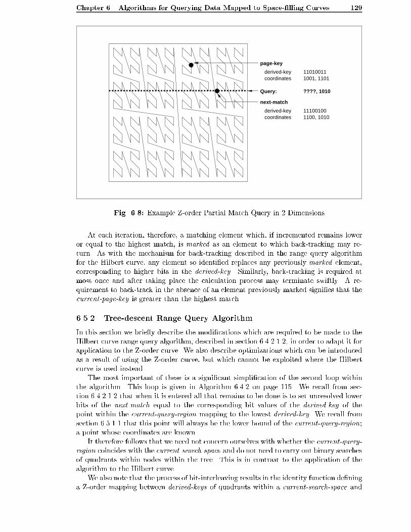
Chapter 6. Algorithms for Querying Data Mapped to Space-�lling Curves 129
derived-key coordinates
derived-key coordinates
page-key
next-match
110100111001, 1101
111001001100, 1010
Query: ????, 1010
Fig. 6.8: Example Z-order Partial Match Query in 2 Dimensions
At each iteration, therefore, a matching element which, if incremented remains lower
or equal to the highest match, is marked as an element to which back-tracking may re-
turn. As with the mechanism for back-tracking described in the range query algorithm
for the Hilbert curve, any element so identi�ed replaces any previously marked element,
corresponding to higher bits in the derived-key. Similarly, back-tracking is required at
most once and after taking place the calculation process may terminate swiftly. A re-
quirement to back-track in the absence of an element previously marked signi�es that the
current-page-key is greater than the highest match.
6.5.2 Tree-descent Range Query Algorithm
In this section we brie y describe the modi�cations which are required to be made to the
Hilbert curve range query algorithm, described in section 6.4.2.1.2, in order to adapt it for
application to the Z-order curve. We also describe optimizations which can be introduced
as a result of using the Z-order curve, but which cannot be exploited where the Hilbert
curve is used instead.
The most important of these is a signi�cant simpli�cation of the second loop within
the algorithm. This loop is given in Algorithm 6.4.2 on page 115. We recall from sec-
tion 6.4.2.1.2 that when it is entered all that remains to be done is to set unresolved lower
bits of the next-match equal to the corresponding bit values of the derived-key of the
point within the current-query-region mapping to the lowest derived-key. We recall from
section 6.5.1.1 that this point will always be the lower bound of the current-query-region;
a point whose coordinates are known.
It therefore follows that we need not concern ourselves with whether the current-query-
region coincides with the current-search-space and do not need to carry out binary searches
of quadrants within nodes within the tree. This is in contrast to the application of the
algorithm to the Hilbert curve.
We also note that the process of bit-interleaving results in the identity function de�ning
a Z-order mapping between derived-keys of quadrants within a current-search-space and

Chapter 6. Algorithms for Querying Data Mapped to Space-�lling Curves 130
the coordinates of those quadrants, expressed as n-points.
This obviates the need to perform mappings from derived-keys to n-points in the binary
searching of quadrants carried out in `step 3' described in section 6.4.2.1.2 and relating
to Algorithm 6.4.3. This is particularly bene�cial in higher-dimensional space where state
diagrams cannot be used for the Hilbert curve. In this binary search operation, we recall
that we must �nd the n-points corresponding to the maximum derived-key of the lower
half of a sub-range of quadrants and the minimum derived-key of the upper sub-range in
order to determine the dimension which divides them.
This simpli�cation is partially but trivially o�set by measures required to accommodate
the fact that adjacent Z-order derived-keys do not necessarily correspond to points which
are adjacent in space, ie consecutive points may di�er in more than one coordinate value.
Where the derived-keys and n-points of the quadrants are in the range
[ lowest,. . . , max-lower, min-higher,. . . , highest ]
the n-point which contains a single non-zero bit corresponding to the dimension which
divides this range into two is evaluated as
(lowest ^ max-lower) � (min-higher ^ highest):
In step 4, the n-point of the quadrant in which we restrict the current-search-space in
the next iteration of the algorithm is required so that we may also restrict the current-
query-region. Again this is available without the need to perform a mapping calculation.
Finally, since the Z-order curve is encapsulated by a state diagram containing a single
state de�ned by the identity function, it is unnecessary to store the state in memory and
the current-state variable is not required.
6.6 Complexity of the Algorithms
In this section, we consider the complexity of the algorithms described in this chapter. The
algorithms fall into 2 categories; the tree-descent approach which is suited to all curves
and the bit manipulation algorithms which appertain speci�cally to the Z-order curve. In
the case of tree-descent algorithms, we do not distinguish between algorithms tailored to
partial match queries and those which are more generally applicable to range queries since
they do not di�er in their complexity.
6.6.1 Tree Descent Algorithms
The complexity of the tree-descent algorithms is, in part, determined by the height of the
tree, which we have already seen in chapter 3 is dependent on the order of the curve, k, or,
equivalently, by the number of bits required to hold any coordinate value. This is re ected
in the total number of iterations of the two loops which comprise the algorithm given in
section 6.4.2.1.2.
In the case of the Hilbert curve or any curve where a state diagram is utilized, a node or
state is visited during each iteration and it is necessary to extract 1 bit from each coordinate
of the range lower and upper bounds or from a partial match query speci�cation. The
complexity of this is determined by the number, n, of coordinates or dimensions which
de�ne a point. Furthermore, we perform a binary search on the values which comprise a
node or state and this too results in a complexity of n. Modifying the query region, in
the case of range queries only, also takes up to n steps. Once a node has been processed,
an additional n bits of the next-match are known but these are placed in the next-match
variable in a single step.

Chapter 6. Algorithms for Querying Data Mapped to Space-�lling Curves 131
Of the operations performed during each iteration, none has a complexity which ex-
ceeds O(n). Thus the overall complexity of the algorithms can be stated as O(kn).
Where Hilbert curve mapping is performed by calculation rather than with the aid
of a state diagram, more work is required but the overall complexity is not increased.
The mappings from derived-keys to n-points which take place during binary searches are
performed in a �xed number of steps, regardless of the number of dimensions. Determining
the characteristics of the next state for the next iteration is e�ected with operations
performed with a complexity of O(n).
Whereas the algorithms can be optimized during implementation for the Z-order curve,
the complexity is unchanged.
In the worst case, it is necessary to perform k iterations of the �rst loop for both
the Hilbert and Z-order curves, followed by a back-tracking to the root which is e�ected
in a single step. Thereafter, the second loop is iterated k � 1 times. Its execution is
considerably simpler than that of the �rst and considerably simpler for the Z-order curve
still but, nevertheless, the complexity of each iteration remains O(n). Thus in the worst
case, the height of the tree is e�ectively doubled.
In the best case, the �rst loop is iterated once only, and back-tracking occurs within it.
Subsequently, the current-query-region is found to be coincident with the current-search-
space prior to executing the second iteration, whereupon the n(k � 1) unresolved lower
bits of the next-match are instantly all set to zero and the calculate next match function
terminates. In this case, the complexity of the search for a next-match is reduced to O(n)
for both the Hilbert and Z-order curves. A best case situation, however, will only be
encountered where query regions are larger than a quadrant of the whole search space.
This is unlikely ever to be the case except, perhaps, in high-dimensional space.
6.6.2 Z-order Bit Manipulation Algorithms
The Z-order curve bit manipulation algorithms described in section 6.5 o�er an improve-
ment in terms of the order of complexity over the tree-descent approach.
In the case of the range query algorithm given in section 6.5.1.2, it can readily be
seen that steps 1, 3 and 4 entail operations of complexity O(n) and that step 5 entails an
operation of complexity O(k) and so the overall complexity is O(n+ k).
The complexity of the partial match query algorithm given in section 6.5.1.3 is deter-
mined by the binary search to �nd the Z-bit. This is determined by the number of bits in
a derived-key, which is (n � k) and so is an operation of complexity O(log(n � k)).

132
Chapter 7
FILE IMPLEMENTATION
We describe in chapters 3 to 5 how n-dimensional points are placed in order along a
one-dimensional interval using a space-�lling curve and how the curve is divided into
contiguous sections corresponding to `pages' of storage. In chapter 6, we describe how
to identify which of these pages intersect with the sections of curve passing through a
hyper-rectangular query region. In this chapter, we describe our practical implementation
in software of a multi-dimensional data storage and retrieval system which utilizes these
techniques and enables data to be held persistently in secondary storage and accessed with
the aid of an index which is compact, exible and simple to maintain.
The �rst 3 sections of this chapter provide an outline of the implementation and
summarize the variations of the concept of mapping data to space-�lling curves which
have been accommodated. These variations principally relate to the choices of curves
used in the mappings and the methods of performing the mappings. In section 7.4, we
focus on details of the format and order in which data is stored on pages. In particular,
for update and query operations, we examine the implications arising from the choices
we make. We examine the reasons why certain choices were made, explain how various
problems were overcome and consider how the application of space-�lling curves impact
on these issues.
In the concluding section, we discuss possible variations to our implementation which
may be pursued as topics for further research. These variations relate to the manner in
which data is partitioned and how pages are referenced in the index.
Our implementation is carried out using the ANSI version of the `C' programming
language except that UNIX system calls are used for �le handling. The replacement of
UNIX system calls by ANSI C equivalents would be a trivial exercise. The implementation
currently runs over the standard UNIX �le management software which would probably
be replaced, were the implementation developed into a commercial product.
7.1 Design Summary
7.1.1 Curves used in the Mappings
Our implementation can be customized to make use of one of a number of space-�lling
curves in mappings between one dimension and n dimensions.
These curves are the Hilbert curve, the two variations of the Z-order curve described
in section 3.7.1, the three variations of the Gray-code curve described in section 3.7.2 of
chapter 3 and our variation of Moore's curve introduced in section 4.3.5.2 of chapter 4.
The choice of curve is made at the time of compiling the source code and cannot be
changed subsequently.

Chapter 7. File Implementation 133
7.1.2 Number of Dimensions
Where mappings to Hilbert and Z-order curves are performed by calculation, our imple-
mentation currently accommodates spaces of up to 16 dimensions but it is not restricted to
this number. We leave an extension of the implementation into higher-dimensional space
as an area for further work.
Where mappings are performed with the aid of state diagrams, however, the number
of dimensions which can be accommodated is restricted by the memory requirements of
the diagrams. A summary of memory requirements is provided in Table 4.4 on page 77.
Thus our implementation functions in up to 8 dimensions using the Hilbert curve, 9 di-
mensions using our variation of Moore's curve and 10 dimensions using the Gray-codeF
curve. In the case of the Gray-codeA and Gray-codeB curves, an upper limit of approx-
imately 20 dimensions applies but we currently accommodate only 16 dimensions in the
implementation.
7.1.3 Order of Curve
All of our program versions utilize curves of order 32. Thus the cardinality of any at-
tribute domain is 232 and any attribute value can readily be accommodated on a com-
puter supporting 32 bit words. This is considered su�cient for most applications. The
implementation could easily be adapted to suit attribute domains of di�erent cardinalities
by making use of variables supported by a compiler of other than 32 bits in size, such as
8, 16, 64 and 128 bits. Since the complexity of our algorithms is in part determined by
the order of a curve, it is clearly advantageous to make use of variables of a size which is
the minimum required.
Our implementation assumes that the cardinality of every attribute domain is the
same. This is equivalent to working in a space which is hyper-cubic in shape. To deviate
from this approach would not be unduely troublesome where the Z-order curve is used in
a mapping but it is less feasible in the case of other curves. Where the cardinality of one
dimension is signi�cantly less than that of another, we have found it advantageous to map
its values to the whole domain which can be accommodated in the variable type used for
the dimension which has the greatest cardinality.
7.1.4 Storage of Data During the Execution of Computer Programs
In our computer programs, the coordinates of a point are held in an array of variables
with each element storing the value of a di�erent coordinate. Since the total number of
bits required to represent the derived-key of a point is the same as the total number of
bits required to represent all of a point's coordinates, it is convenient also to hold the
derived-key in an array of the same type and size. This imposes a small overhead in that
bitwise manipulation of a set of n bits within a derived-key may require processing of some
most signi�cant bits of one array element together with some least signi�cant bits of the
next higher array element but for the most part this is unavoidable. An exception would,
for example, be where we are using a 4-dimensional curve of order 16 where a derived-key
could be held in a single 64 bit word.
Because of the extensive use of bit manipulation employed in our algorithms, we exclu-
sively use variables of the unsigned integer type. As a result of this, any attribute domain
which comprises values of a di�erent type, such as signed integers or real numbers, must
be mapped to unsigned integers. This can be facilitated by the application of a lexical
token convertor, as noted below in section 7.3.

Chapter 7. File Implementation 134
7.1.5 The Data File
A data �le comprises a set of �xed length pages of data. The capacity of a page is
predetermined at compile-time and cannot be altered subsequently. Each page represents a
section of curve and holds all of the datum-points lying on that section. The lowest derived-
key corresponding to a datum-point which is placed on a page becomes the page's index
entry, called the page-key, together with the page number. If the point is subsequently
deleted, it is not necessary to alter the index entry for the page. The page corresponding to
the �rst section of the curve is indexed with the derived-key of zero, regardless of whether
it corresponds to a datum-point.
Page numbers are assigned in the sequence in which pages are created and there is no
relationship between the ordering of page numbers and the ordering of contiguous sections
of curve. If a page is deleted, its page number is placed in a list of page numbers which
are available for re-use. The physical page is not deleted from the �le but instead it is
e�ectively marked as being deleted since the index will contain no entry for it. If no free
pages are available then any new page is assigned a number which is one greater than the
last new page number which was generated previously.
A page of data comprises a set of coordinates of datum-points, rather than their derived-
keys. The coordinates of a point are ordered according to the ordering or numbering of
the dimensions in a space. In our application, we order data on a page in a consistent
manner. For example, if the dimensions are numbered 1; 2; : : : ; n then we order points �rst
by coordinate values in dimension 1. Datum-points with the same values in dimension 1
are ordered by values in dimension 2 and so on. The reasons for ordering data and the
alternatives to it are also discussed in more detail in section 7.4.
The mapping techniques employed ensure that data in a �le is, in e�ect, fully and
exibly indexed on any combination of coordinate values. In addition to the data held
as coordinate values, a page of data may optionally contain non-indexed data associated
with each point. Whether such data is to be stored and the amount of such data must be
determined at compile-time and it cannot be altered subsequently.
7.1.6 The Index
The purpose of mapping data to one dimension is to be able to index it using concepts
which are suitable for one-dimensional data. Any one-dimensional indexing method is
suitable and we choose to use the B+-Tree.
In our implementation, the index is held in a separate �le. The entire index is read
into memory on opening of the data store and it is written back to the �le when the data
store is closed, if it has been updated. The implementation could easily be extended so
that not all of the index needs to reside in memory should its size dictate.
7.1.7 Main Memory Bu�er
Data is held persistently in a �le which is maintained in secondary storage. On opening
the �le, an area of primary storage is allocated as a bu�er. This bu�er has a predetermined
capacity to hold a �xed number of pages of data from the �le. The bu�er capacity may
be varied for a particular �le but changes to it require recompilation of the program
executable.
A B+-Tree index, separate to that used for indexing the data �le, is maintained in
memory to record which pages reside in the bu�er at any particular time. If a page
is required to be accessed and it is not currently contained in the bu�er then the least
recently used page which is in the bu�er is swapped out. This may entail updating the
�le store if the contents of the page have been changed since it was last read from the

Chapter 7. File Implementation 135
�le. A ag indicates whether the page has been updated and a variable associated with
each page in the bu�er keeps track of the sequence in which pages are read from the �le.
Alternative strategies to the least recently used one could be implemented.
An additional ag is stored for each page in the bu�er to indicate whether it is currently
in use, ie is being searched, as part of the execution of a query. This ag is intended to
avoid pages being swapped out of memory or being merged with other pages if they are
being searched.
7.1.8 Ancillary Files
Associated with each data �le and its index �le are two additional �les. The �rst of these
contains a list of free pages within the data �le, if any. The second �le contains meta-data
such as the number of free pages, the highest page number which has been assigned to
date and information on page size, curve type and the number of dimensions relating to
the data �le. Some of this information is used to verify the compatibility between the data
�le and the executable program �le which opens it for data processing.
7.1.9 Query Execution Strategy
We adopt a similar strategy for the management of the processing of queries to that used
by Derakhshan in his Grid File implementation [Der89] which enables a number of queries
to be executed concurrently. An upper limit on how many queries may be processed
concurrently is, however, speci�ed at compile-time but this may be changed during the
lifetime of a data store, simply by changing a parameter and re-compiling the source code.
An array of numbered blocks of memory, called retrieval-sets, is allocated to hold
information on all queries which are active at any particular time. When a query is
invoked, the array is searched in order to �nd a block which is not already in use by
another query. If no such block is found then the query cannot proceed. When an unused
block is found, it is reserved for use by the query for the duration of its execution. The
query is assigned a retrieval-set identity number which is the array element number of the
memory block.
Information stored about a query in its retrieval-set block includes the speci�cation
of the query, the location of the page in the bu�er which is currently being searched for
matches to the query and the location on the page of the next record to be examined.
Additional information which aids the detail of the implementation is also stored, such as
a count of the number of unspeci�ed coordinates in a partial match query.
7.2 The Application Interface
The implementation of our work comprises low level software which is intended to provide
facilities, in the form of a set of functions, for use by higher level applications. No user
interface exists and the responsibility for providing one, if required, lies with the higher
level applications.
In this section we summarize the functions which are provided and which enable an
application to create, update and query a data store. Function names are given and
parameters passed to them are in parenthesis.
db create (database-name) This creates a new database, including all of its ancillary
�les. An empty page with a page-key of zero is placed in the data �le and an entry
for it is made in the index. The free page list is initially empty. Once created, the
database is closed.

Chapter 7. File Implementation 136
db open (database-name) Opens a database for updating and querying. The index is
read into memory from �le and main memory is reserved for use as a bu�er.
db close (database-name) Causes the database to be closed. The bu�er is scanned to
check whether any modi�cations have been made to any page but not yet written to
the �le store. The index is rewritten to �le and the free page list data is also written
to �le.
db data insert (datum-point) Inserts a datum-point into the database. A return value
of zero indicates that the datum-point is already present, otherwise a non-zero return
value signi�es successful insertion. A non-zero return value also represents the page
occupancy following an insertion and may trigger a page split, but this is transparent
to the application which calls the function.
db data delete (datum-point) Deletes a datum-point from the database. A return
value of zero indicates that the datum-point was absent to begin with, otherwise
a non-zero return value signi�es successful deletion. A non-zero return value also
represents the page occupancy following a deletion and may trigger action to resolve
underpopulation, again transparently to the application which calls the function.
db open set (partial-match-query, set-number) This identi�es a free retrieval-set
element if one exists and initializes it in accordance with the partial match query
speci�cation. The set number is placed in the second parameter. The function's
return value indicates whether a free retrieval-set was found.
db fetch another (set-number, datum-point) This lazily searches the database for,
at most, a single match to the partial match query, the details of which are stored
in the retrieval set element with number `set-number'. The return value indicates
whether a match was found, in which case the results are placed in the datum-point
parameter, or whether no further matches are to be found. The function is called
once for every datum-point retrieved and once when it signi�es no further matches
are to be found. A single call to the function may result in the searching of more
than one page of data.
db close set (set-number) This releases a retrieval-set block of memory for use by
another query.
db range open set (range-query, set-number) This is similar to db open set but
applies to range queries.
db range fetch another (set-number, datum-point) This is similar to db open set
but applies to range queries.
7.3 Use and Compatibility with other TriStarp Group
Software
The research described in this thesis has been carried out within the Triple Store Appli-
cations Research Project (TriStarp) of the Department of Computer Science at Birkbeck
College. Previous work carried out within this Project includes the development of a num-
ber of functional programming languages for use with functional databases [Ayr95, Mer99,
Pou89, Sut95]. Data storage facilities are currently provided by Derakhshan's [Der89] im-
plementation of the Grid File [NHS84].

Chapter 7. File Implementation 137
The data storage application developed and implemented in this thesis may be used
as an alternative to the existing Grid File. The functionality of the interface to our imple-
mentation is similar to that of the existing Grid File, but it di�ers in detail, principally in
our use of unsigned integers rather than signed integers.
In order to use and test our software under higher level TriStarp applications, we
have created a set of `wrapper' functions which have names, parameters and return value
types which are identical to those provided by Derakhshan. These functions call functions
provided within our implementation and act as an interface between the latter and higher
level software.
Provision of this interface results in a number of bene�ts. We are able to demonstrate
empirically the correct functioning of our application which can be tested with a variety
of data sets used in the research and teaching activities of the TriStarp Group. The use of
TriStarp Group languages over our application entails subjecting it to a realistic variety of
updates, both insertion and deletion. Our application is only tested in 3 and 4 dimensions,
however, when used by higher level TriStarp Group software.
In practical data storage applications, not all of the attributes of records of data are
necessarily integers; for example they may be real numbers or strings of characters. Thus
where a data storage implementation holds all values as integers, a facility is required
which maps non-integer values to integers. Derakhshan achieves this by utilizing a lexical
token convertor [LW84] and this approach is equally suitable for our implementation and,
indeed, other methods such as the original Grid �le and the BANG �le [Fre87].
Since the existing TriStarp Grid File utilizes a lexical token convertor, we have incor-
porated its implementation in software into our own implementation where the latter is
used under existing higher level TriStarp applications. Thus our implementation may be
used transparently with the high level software.
7.4 Implementation Details
In carrying out an implementation, various issues of detail need to be resolved. In some
cases they con ict and, certainly, they in uence each other. An obvious example is that
any �le organization design must accommodate the requirement to update a data store
whilst also providing an optimum environment for facilitating the selective retrieval of
data.
In section 7.1, we provide a summary of the implementation of our design and in this
section we explore the implications of some of the decisions and consider some of the
alternative options which were rejected. We also elaborate on the detail of how some
operations, such as page splitting and merging, are performed and how the use of space-
�lling curves impact on these operations.
The choice of the format in which data is stored and the order in which it is stored
are intimately related and they impact both on the manner in which page searching is
performed and how an e�cient page utilization is maintained. This is true for any method
of �le organization but where space-�lling curves are used it appears that there is a greater
choice of combinations of format and order.
If data is not maintained in some order on a page then the cost of searching a page
which may contain data which matches some query speci�cation is expensive since every
data value on it must always be examined to determine whether it is a match. Furthermore,
insertions require a serial search of the whole of a page to ensure a data value is not already
present before it is appended. Similarly, deletions will on average require a serial search of
half of a page to locate any record to be removed, provided it exists. On the other hand,
maintenance of data in some order also imposes an overhead in terms of work required.
In common with all �le organization methods, it is desirable to ensure that all pages

Chapter 7. File Implementation 138
of data contain a minimum of free space otherwise the ratio of the volume of data to the
size of the data �le degenerates and the index size increases unnecessarily. To maintain a
high page occupancy there must exist satisfactory mechanisms to divide a page into two
pages when its data occupancy has reached its `capacity', to merge two adjacent pages
into a single page when their combined occupancy falls below the capacity of a single page
and to move data to an underpopulated page from a neighbouring page when the two
adjacent pages hold more data than can be stored on a single page. At the same time it
is desirable to set thresholds in such a way that redistribution of data is delayed to some
extent otherwise periods of high activity in terms of both insertion and deletion can give
rise to unnecessary page splitting and merging.
The term underpopulated relates to a page whose occupancy has fallen below some
arbitrary threshold, typically about 50% of potential capacity. A higher threshold could
be set in an attempt to maximise storage utilization but clearly as soon as a page is
divided into two, its replacements would be underpopulated and some mechanism would
be required to prevent an immediate redistribution of records between neighbouring pages.
In exploring the implications of the details of an implementation we �rst consider the
case where data is stored in derived-key format, and then consider the case where data is
stored as sets of coordinates of datum-points.
7.4.1 Storing Data as derived-keys
In this section, we �rst consider the implications of storing derived-keys sorted in order
on pages, and then the implications of not maintaining any order.
7.4.1.1 Ordered Data
When data is stored as a sorted list of derived-keys, in searching a page during query
execution, it is possible to perform a binary search of the page to determine the point at
which the page search begins. This is irrespective of whether the query type is a range
query or a partial match query and, in the latter case, regardless of which coordinates are
speci�ed. This is an e�cient way of �nding the next-match on any page, if it corresponds
to a datum-point.
In order to �nd subsequent matches, two alternative approaches are available. The
�rst is to search the page serially, beginning from the position where the search for the
lowest derived-key terminated, whether or not this search resulted in �nding a match.
Each derived-key is mapped to its corresponding n-dimensional set of coordinates, and
these are compared with the query speci�cation to see if the datum-point lies within the
query region. This entails an operation of complexity O(kn) to perform each mapping
followed by an operation of complexity O(n) to determine if a match is found.
The second approach is to execute the calculate next match function, described in
chapter 6, to calculate the value of the next-match which might exist and then perform
a binary search on the rest of the page to �nd whether it is present and then repeat this
process until it is found that no higher match can possibly exist on the page.
We have seen that �nding the next-match is an operation with a complexity of O(kn).
How many times this function would need to be called and followed by a binary search
of the remaining records on the page, depends on the distribution of data on the page
and this is not predictable. Only when a next-match is found to exist on a page would
a mapping calculation be required in order to return its corresponding datum-point. In a
worst case situation, it would be necessary to call the next-match function and perform
a binary search for every record on the page following the position of the �rst possible
match.

Chapter 7. File Implementation 139
When required as a result of performing updates on a data store, moving data from
one page to another would be trivial where data is stored as derived-keys. Where a page
must be split into two, we simply move the bottom half of a full page to the head of
a newly created page. Merging two pages entails appending the contents of one to the
other. Similarly, moving records from a page to an underpopulated neighbour entails the
transfer of a contiguous block of records from the former to the beginning or the end of the
latter. Records may need to be moved to make room for additions to a page and any gaps
created would need to be closed up, depending on whether records moved to a preceding
or succeeding page.
Data updating would require moving contiguous blocks of records to make room for a
new record inserted or to close up a gap after a deletion.
7.4.1.2 Unordered Data
Where data is unordered, the only operation which can be carried out in a relatively simple
manner is the merging of two adjacent underpopulated pages. Page merging entails the
moving of a block of derived-keys from one page to the end of another.
A newly inserted derived-key is simply placed at the end of a page but before doing
so, it is necessary to examine each of the existing derived-keys on a page to ensure that
the derived-key to be inserted is not already present. Deletion of a derived-key entails a
serial search of the page to locate it. Gaps created by deletion can be �lled simply by the
last record on a page.
Each search to �nd matches to a query requires a serial pass through the whole of a
page, mapping each derived-key to its corresponding datum-point encountered.
Splitting an overpopulated page requires �nding the median value on the page and then
extracting derived-keys greater in value and moving them to the new page, closing up gaps
on the original page as required. More is said in a later section in this chapter about �nding
the median derived-key on a page. Moving data from a page to an underpopulated page
poses similar problems.
7.4.2 Storing Data in Coordinate Format
In this section we consider the case where we store data as sets of coordinates. Unless
stated otherwise, we assume that the coordinates are stored in the same order as is used
to specify queries. We also assume in the case of the Z-order curve, that the coordinates
are stored in the same order in which bits are taken from coordinates and interleaved in
order to generate Z-order derived-keys.
7.4.2.1 Ordered Data
Where data is ordered by coordinate value, page searching proceeds in the same way for
applications implemented over space-�lling curves as it does for some other methods such
as the existing Grid File implementation currently used by the TriStarp Group.
The speci�cation of a range query allows, for any page intersecting with the query, a
binary search to be performed to locate the position where the �rst possible match will
be stored on the page, if it is a datum-point. The same is true of partial match queries
but only where at least the `�rst' coordinate is speci�ed, otherwise a serial search of the
whole page is necessary.
Following a binary search, the page is then searched serially until a datum-point is
found which is not a match to the query. Subsequently, the next matching datum-point, if
it exists, is found either by performing another binary search (if possible) or by continuing
with a serial search.

Chapter 7. File Implementation 140
Page searching can sometimes be terminated before the end of the page is reached. As
soon as a datum-point is found whose `�rst' coordinate is greater than the `�rst' coordinate
of the query range upper bound, then no further matches can exist on the page. Where
a mapping to the Z-order curve is used, this condition arising also signi�es completion of
the query process, but in the case of other curves further matches may still be present
on other pages. Similarly, if the �rst i, i < n, coordinates of a datum-point are all equal
to the corresponding range upper bound coordinates but coordinate i + 1 is greater in
value, then no further matches exist on the page. Terminating the search in this way is
not possible where data is ordered by derived-key value, except where a search is made of
the last page which may contain matches to the query.
Reorganizing data by moving it from one page to another is, however, more problematic
where space-�lling curves are employed and where data is stored, in order, as sets of
coordinates rather than as derived-keys. The simplest case is where pages are merged but
the datum-points do need to be interleaved on a new combined page to maintain them in
order and we are unable simply to copy a block in a contiguous manner.
Where a page is to be split, its datum-points need to be partitioned into two halves
such that the derived-keys of those in one half are lower than those of the other. However,
there is not generally any correlation between the position of a datum-point on a page
and the value of its derived-key. We address this problem by determining the approximate
median derived-key of the datum-points about which the latter are partitioned. This is
discussed further in section 7.4.3 below. Moving data to an underpopulated page from an
adjacent page presents a similar problem to that faced when splitting pages. Problems of
a di�erent nature exist for other existing �le organization methods and we discuss some
of these further in chapter 8.
As with datum-points stored as derived-keys and in sort order, existing datum-points
must be moved to accommodate an insertion and gaps must be closed following a deletion.
Locations for insertion and deletion are determined by binary searching and so determining
whether a datum-point to be inserted is already present is trivial.
7.4.2.2 Unordered Data
Where data is stored as sets of coordinates but not stored in order on a page, we su�er
almost all of the disadvantages encountered above with the most notable exception being
that page merging is as simple as described in section 7.4.1.2.
Serial searching of the whole page is always required during querying and before inser-
tion can take place although new data is simply placed at the end of a page. Identifying
which records to move from one page to another during page splitting or data redistribu-
tion entails resolving similar problems to those encountered in section 7.4.2.1.
7.4.3 Redistribution of Data Stored in Coordinate Format and in Sort
Order
In this section we describe our technique for redistributing some data from one page to
another, where the data is stored in coordinate format and maintained in sorted order.
The need for this occurs in two situations; �rstly, where a page must be split into two
because its data occupancy has reached its capacity and, secondly, where data must be
moved from one page to a neighbouring page which has become underpopulated. We
discuss the two situations separately although they are related. We do not discuss the
merging of two pages into one as this is a relatively trivial operation.

Chapter 7. File Implementation 141
7.4.3.1 Page Splitting
When datum-points are stored on a page in attribute order they are sorted according
to their derived-keys under a mapping to the `Scan' curve, described in section 3.7.3 of
chapter 3. Clearly, where any other curve is used, they are not stored in derived-key order.
In order to divide a page into two, we must therefore calculate the derived-keys cor-
responding to all of the datum-points and then determine the median of these values.
Datum-points which map to derived-keys which are less than the median remain on the
original page and all others are placed on the new page. Once the page has been split,
datum-points on both the original and new pages must be ordered according to their
attribute values.
In our implementation, the derived-keys, once calculated, are initially placed on a
temporary page of storage. An obvious way of determining the median would be to sort
the derived-keys but this operation would be computationally expensive, especially given
that a page of data may contain thousands of datum-points.
As an alternative to sorting derived-keys, we explored the option of �nding the ap-
proximate median by using a median-of-medians algorithm. This is an iterative technique
and begins by dividing a set of i values into j sub-sets each containing m values, where
j = i=m and m is a small odd integer, typically 3, 5 or 7. Each of the sub-sets is then
sorted, at little cost, and a set of j median values are found, one taken from each sub-set.
In the next iteration, we repeat the process but begin with a smaller set of values where
i = j and the members of the set are the medians found in the previous iteration. The
process continues until the set of values under consideration contains only m members
and its median is the approximate median of the original set of values. The number of
iterations required equals logm i.
We carried out experiments populating data stores with randomly generated data
and setting m variously to 3, 5 and 7. In some experiments datum-points were stored
in coordinate value order and in others they were stored in no order. We noted that
where datum-points were stored in a random or arbitrary order, the median-of-medians
technique generally found medians which were closer to the true medians. As a result,
the data stores created generally contained fewer pages since, when pages were split, they
were divided more evenly. It appears that when datum-points are ordered by coordinate
value a partial ordering by derived-keys results, and to some extent this frustrates the
process of calculating an approximate median.
In order to improve the balance of page splitting where datum-points are sorted by
coordinate value, we place the calculated derived-keys in randomly chosen positions on
the temporary page referred to above. This simulates a random ordering of datum-points
on the original page. This strategy enables us to achieve similar results in terms of �nal
�le size for sorted data as we had achieved with unsorted data.
As a �nal re�nement, once the median-of-medians process has reduced its set of working
data to between 30 and 50 median values, then rather than continue we simply sort these
values and take their median as the approximate median. In experiments, this approach
was also found to result in identifying approximate medians which are closer to true
medians of a set of derived-keys.
7.4.3.2 Moving Data to Underpopulated Pages
Determining which datum-points to move from one page to an underpopulated neighbour
proceeds in a similar manner to that described in the previous section except that we need
to �nd the approximate median derived-key of all of the datum-points on both pages. In
describing the technique, we assume that the underpopulated page is the successor of the
page from which datum-points will be moved, although the reverse situation is equally

Chapter 7. File Implementation 142
possible and handled in a similar manner.
Initially, it would appear that �nding the approximate median of two pages of data
entails twice as much work as �nding the median of a single page. Nevertheless, when
we move data to an underpopulated page, the combined occupancy of the two pages
participating in the process will never exceed the sum of the capacity of one page plus the
minimum allowed occupancy of a page. Furthermore, we know that the median cannot lie
on the underpopulated page. Where the latter is the successor page, we also know that
all of the datum-points on it must map to derived-keys which are greater than the median
and thus we are able to disregard their actual values and assume instead that they are
arbitrarily high. It is therefore unnecessary to perform any median calculations relating to
datum-points on the underpopulated page, thus simplifying the procedure. Having found
the approximate median, which will be on the larger page, we transfer datum-points which
map to this derived-key and higher derived-keys to the underpopulated page in a manner
such that records on both pages are maintained in coordinate value order.
7.4.3.3 General Procedure for Dealing with Underpopulated Pages
The techniques described in the previous section leads us to adopt the procedure given
in Algorithm 7.4.1 when dealing with pages which have become underpopulated following
record deletion. It can be seen that this is no di�erent from that which is applied to
one-dimensional data.
Algorithm 7.4.1 Procedure for Dealing with Underpopulated Pages
1: if the page is underpopulated then
2: if the page has a predecessor then
3: retrieve the predecessor page
4: if the combined capacity of the underpopulated page and its predecessor is less
that that of a single page then
5: merge the underpopulated page and its predecessor
6: delete the underpopulated page from the index
7: else
8: move some records from the predecessor to the underpopulated page
9: update the index entry for the underpopulated page
10: end if
11: else
12: retrieve the successor page
13: if the combined capacity of the underpopulated page and its successor is less that
that of a single page then
14: merge the underpopulated page and its successor
15: delete the successor page from the index
16: else
17: move some records from the successor to the underpopulated page
18: update the index entry for the successor page
19: end if
20: end if
21: end if
An advantage of our approach to indexing of multi-dimensional data is that it is pos-
sible to experiment and implement a variety of alternatives to this strategy. One example
would be to always attempt to perform a page merge as a �rst priority. We conjecture,
however, that the opportunity to merge two adjacent pages would occur relatively rarely.

Chapter 7. File Implementation 143
This strategy would, therefore, probably almost always entail retrieving both the prede-
cessor and the successor of an underpopulated page and ultimately result in moving data
from one of an underpopulated page's neighbours anyway. Thus the overhead of possibly
reading an additional page into memory, if it is not already present, would not be worth-
while. Our strategy, therefore, gives priority to merging an underpopulated page with its
predecessor or moving data from the latter.
7.5 Potential Variations to the Indexing Implementation
The particular querying experiments carried out, using random data, and reported on
later in chapter 10 found fewer pages required to be searched where data is held in the
Grid File, rather than in our storage application.
Although the number of pages searched is not the only factor of importance in compar-
ing the two �le organization approaches, we are motivated to investigate whether strategies
exist for improving the performance of our implementation which are not available to the
Grid File. We therefore consider two variations for determining what derived-key val-
ues are stored in an index, which we investigated at a preliminary level. We also brie y
consider the application of B�-Tree concepts to page splitting and reorganization in our
implementation.
We believe these variations to be worth considering as part of a programme for future
work. They entail the carrying out of more work during updating operations but they are
intended to facilitate querying. We see in chapter 10 that there is a case to be made for
improving the e�ciency of querying at the expense of updating since the former is the
more costly operation.
7.5.1 Indexing Intervals
The indexing method we have hitherto described envisages partitioning a space-�lling
curve into contiguous but variable length sections, on each of which lies a set of datum-
points of roughly the same size which is stored on a distinct page in a data �le. We have
seen that the derived-key of the �rst datum-point which is placed on a page determines
its page-key, even if the datum-point is subsequently deleted.
In any database, the datum-points are likely to be a very sparse sub-set of all of the
points which lie on a space-�lling curve and so it follows that there will be many sections
of curve on which no datum-points lie at all and that many of these may be `long'. It is
also probable that there will often be many points which will map to derived-key values
which lie between the highest derived-key of a datum-point on a page and the page-key of
the succeeding page.
These observations lead us to an alternative approach in which we consider a page
of data as being a section of curve bounded at both ends by the derived-keys of actual
datum-points rather than being bounded at the start by a page-key and bounded at the
end by a value equal to the succeeding page's page-key minus one.
This alternative approach, therefore, envisages that an index entry for a page comprises
of a pair of page-keys rather than a single one. It enables us to infer from the index some
of the sections of curve on which no datum-points lie and so this may allow us to reduce
the number of pages which must be searched in the execution of a query.
Once a page has been searched, we calculate the next-match which is greater than or
equal to the �rst page-key of its succeeding page. We then look in the index to see whether
the next-match lies between the pair of page-keys for a page and if it does, we retrieve and
search the page in the normal manner. If, on the other hand, the next-match lies between
the second page-key of a page and the �rst page-key of its succeeding page then we do

Chapter 7. File Implementation 144
not need to retrieve any page at this stage and, instead, we perform a further next-match
calculation on the �rst page-key of the succeeding page. We continue in this way until we
either �nd a next-match which lies between a page's page-keys or until we �nd there is no
higher match to the query.
The penalties which are associated with this approach relate to index maintenance.
The most obvious implication is that the index size is almost double that of the method
described previously, since a page requires two page-keys instead of one.
If a datum-point is inserted into the data store and its derived-key does not lie between
a page's page-keys, then we must decide which of two possible pages to place it on and
update one of that page's page-keys in the index to suit.
If a datum-point is deleted, we must check to see if its derived-key is a page-key for the
page it is stored on and, if so, examine the other datum-points on the page, calculating their
derived-keys in the process, in order update the appropriate page-key for the page. This
task would clearly be simple if data is stored in derived-key order but not if data is stored
in coordinate order unless an index is held on a page to map datum-point locations to their
derived-key order. Nevertheless, such an index would be relatively compact, occupying
one or two bytes times the number of datum-points which can be stored on a page. The
relative cost of such an index, as a proportion of the size of a data �le, decreases as the
number of dimensions in space increases.
A further complication which we may choose to address is that a page may overlap
longer sections of curve on which lie no datum-points than exist between pages. This
invites consideration of the potential for maximising the lengths of curve sections which
lie between pages by judiciously moving datum-points from a page to one of its neighbours.
We performed some limited experiments with randomly generated data on a variation
of our software which implements the concept of indexing pages with pairs of page-keys
which are updated as records are inserted and deleted but did not �nd the results to be
very promising. On re ection, this is perhaps not surprising where random data is used
since the length of a curve section which lies between two pages is typically no longer than
a curve section which lies between any pair of datum-points. This leads us to speculate
that the concept is more likely to prove bene�cial in an application where data is highly
and multiply clustered.
7.5.2 Adjusting Page-key Values to In uence Page Shape
We note that partitioning space by dividing a space-�lling curve into sections can result in
sub-spaces with lower volume to surface area ratios than sub-spaces created by the Grid
File and having similar minimum lower bound and maximum upper bound coordinate
values. These sub-spaces can have convoluted boundaries which, in turn, can result in
hyper-rectangular query regions intersecting with more pages than where sub-spaces are
themselves also hyper-rectangular. This is illustrated by example in Figure 7.1.(a).
By moving certain datum-points from one page to an adjacent page the `shapes' of the
pages are changed and it is sometimes possible to coerce them into forms which are more
hyper-rectangular. This can reduce the number of pages which intersect with a query
region and is illustrated in Figure 7.1.(b) in which one datum-point has been moved from
page number j to page number j � 1 for 1 < j � 4.
We note that if all of the page-keys in an index had values of zero in their bottom i
bit positions, where i is an arbitrary number, then the partitioning would in e�ect result
in a set of hyper-cubes. Such a partitioning is likely only to be achieved in practice where
data is randomly distributed and where a page size is chosen fortuitously.
Nevertheless, it would be possible to attempt to index pages with page-keys which
contain as many zeros as possible in lower bit positions. Such page-keys would, in general,

Chapter 7. File Implementation 145
page-key
datum-point
Key
Page No.
P1
P2
page-key
P4
00000000
00111110
01111010P3
Example (a)
Page No. page-key
P1
10110100
P3
P4
00000000
01000000
10000000
11000000
Example (b)
page boundary
P2
query region
(a)
P1
P2
P4
P3
(b)
Fig. 7.1: Example showing how the choice of page-key a�ects page shape
not correspond to datum-points placed on pages. In order to determine these page-keys,
the only information required in addition to that which is available in our standard im-
plementation would be the highest derived-key of any datum-point on a page. A page's
page-key would then be a value which lies between the lowest derived-key of any datum-
point on it and the highest derived-key of any datum-point on the preceding page. As in
the previous section, it would be necessary to keep track of the highest derived-key of a
datum-point on a page during updating but the index size would remain the same as in
our standard implementation.
7.5.3 The Application of B�-Tree Concepts
Our data store design utilizes a B+-Tree index to organize pages of data but such a
distinction between index and data is arbitrary and the data pages may be considered
simply as leaf nodes of a B+-Tree.
This notion encourages us to consider the application of characteristics of variations to
the B-Tree, other than those of the B+-Tree, in managing page splitting and merging on
the insertion and deletion of data. For example, the B�-Tree, attributed to Knuth [Knu73]
and discussed by Comer [Com79], is of particular interest since it guarantees a minimum
node occupancy of 66%, compared with 50% for the B+-Tree. This is achieved by delaying
page splitting. When a page is fully occupied, instead of it being split into 2 pages, data

Chapter 7. File Implementation 146
is transferred to a sibling node. When both siblings are full, they are divided into 3 pages,
each with an average data occupancy of 66%. This strategy could be readily applied to
page splitting (and page merging) within our implementation and thus potentially result
in more compact data stores (and indexes) requiring fewer pages to be searched in the
execution of queries.
7.6 Concluding Remarks
In this chapter we have described our implementation of the concept of using a mapping
to a space-�lling curve in an application for the storage and retrieval of multi-dimensional
data. This implementation comprises a number of component parts addressing di�erent
requirements of the application. To varying degrees these parts in uence each other or
they are independent of each other.
Particularly where they are independent of each other, scope exists to vary the imple-
mentation and such variations may impact on its performance. During the course of our
research it has been necessary to make considered choices but we cannot be certain that
these have, in all cases, been optimum choices. Determining this is an area for further
research and the observations we make in section 7.5 suggest a number of directions this
research might take.

147
Chapter 8
COMPARISON WITH OTHER FILE
ORGANIZATION METHODS
In chapter 2 we summarize previous work relating, inter alia, to the organization of multi-
dimensional data. In this chapter we return to this subject, having described our approach
and its implementation, in order to compare it in some detail with two other well known
approaches; the Grid File and the BANG File. In particular we focus on some of the
implications of the design strategies for issues such as index growth, page occupancy,
what is stored on a page and how updates are managed.
8.1 The Grid File
The Grid File is a method for partitioning multi-dimensional space proposed by Nievergelt
et al [NHS84] which has been the subject of considerable interest and which we found to
be the most frequently cited in research literature on the subject. It forms the basis for
the existing Triple Store implementation utilized by the TriStarp Group.
8.1.1 The Index
We noted in chapter 2 that a drawback of the Grid File is the exponential growth rate of
its index size and a need for periodic substantial index reorganization. Ameliorating this
was the principal contribution of the research carried out by Derakhshan [Der89] but, in
our view, problems remain and these contribute to the motivation for our research. They
relate to the amount of reorganization that is required to the index when a data store
is updated, the growth in size of the index as data is added, the con icts which arise in
determining the way pages are divided and the manner in which pages are identi�ed for
searching in the execution of a query.
We recall that in the Grid File design, a page of storage corresponds to a hyper-
rectangular sub-space of the key-data domain and that a hyper-rectangle is de�ned by
n sub-intervals, one for each dimension. A sub-interval in dimension d is delimited by a
lower bound and an upper bound value in dimension d.
Derakhshan's system for indexing these sub-spaces comprises 3 principal components
called E-Scales, S-Modules and R-Modules. A simple 2-dimensional example is shown in
Figure 8.1.
An E-Scale exists for each dimension and comprises a list of the sub-intervals into
which a dimension has been divided. A division exists in an E-Scale for dimension d if at
least one page has been divided on dimension d. If all sub-spaces span the whole domain
in some dimension d then the E-Scale for that dimension is not divided and contains a
single entry.
For each entry or sub-interval which exists in an E-Scale for dimension d, the S-Module
contains an S-List which is a list of the identi�ers of all of the pages or sub-spaces which
intersect with the sub-interval in dimension d. If a page spans more than one sub-interval

Chapter 8. Comparison with other File Organization Methods 148
P1
P2
P3
P4
P5
P6 P8
P9P7
0 25 50 75 100
0
25
50
75
100
[0, 25)
[25, 50)
[50, 75)
[75, 100)
P1, P2, P3, P4
P5, P6
P7, P8
P8, P9
E-scale E1 S-records
[0, 25)
[25, 50)
[50, 75)
[75, 100) P4, P6, P8
P3, P6, P8
P2, P5, P7, P9
P1, P5, P7, P9
E-scale E2 S-records
P1
P2
P3
P4
P5
P6
P7
P8
P9
[0, 25)
[0, 25)
[0, 25)
[0, 25)
[0, 25)
[25, 50)
[50, 75)
[75, 100)
[25, 50)
[50, 75)
[25, 50)
[75, 100)
[50, 100) [50, 100)
[50, 100)
[0, 50)
[0, 50)
[0, 50)
E2E1Page
R-module
E2
E1
Data-space partitioned into pages
Fig. 8.1: Example of Derakhshan's Grid File Index

Chapter 8. Comparison with other File Organization Methods 149
P4, P8, P10
P4, P6, P8
P3, P6, P8
P2, P5, P7, P9
P1, P5, P7, P9
S-records
[25, 50)
[50, 75)
[75, )
[90, 100)
90
E2E1
E-scale E2
R-module
P10 [25, 50)
[0, 25)
P1
P2
P3
P4
P5
Page
P7
P8
P9
[0, 25)
[0, 25)
[0, 25)
[0, 25)
[0, 25)
[25, 50)
[50, 75)
[75, 100)
[25, 50)
[50, 75)
[25, 50)
[75, 100)
[50, 100) [50, 100)
[0, 50)
[0, 50)
[0, 50)
[50, )90
[90, 100)
[0, 25)
[25, 50)
[50, 75)
[75, 100)
P6
E-scale E1 S-records
P1, P2, P3, P4
P7, P8
P8, P9
P5, P6, P10
P10
E2
E1
0 25 50 75 100
0
25
50
75
100
P1
P2
P3
P4
P5
P6 P8
P9P7
90
Alterations required to indexarising from the division of page P6
Fig. 8.2: Example showing the implications of a page-split in the Grid File
into which a dimension has been divided then its identi�er appears in more than one
S-List.
The R-Module is a list of page identi�ers and their corresponding pairs of lower and
upper bound coordinate values in each dimension.
In Figure 8.2 we show an example of updates required to the components of the index
if an existing page, P6, is divided into two disjoint sub-spaces, with page identi�ers P6
and P10, along a boundary in a dimension which requires the division into two of an
existing sub-interval in an E-Scale.
Changes required to the index are as follows:
1. A new entry is added to the E-Scale for dimension y.
2. The interval for the original entry is rede�ned.
3. A new S-List is created for the new entry which is identical to the original except it
contains the identi�er for page P10 instead of P6.
4. One S-List for all other dimensions, just one in our 2 dimensional example, is updated
to include the new page.
5. The entry for P6 in the R-Module is updated and an entry for P10 is added.

Chapter 8. Comparison with other File Organization Methods 150
Had the boundary between pages P6 and P10 in dimension y coincided with that
between pages P3 and P4 then less work would have been required: steps 1-3 would
have been replaced by simply updating the S-List for the sub-interval in the dimension y
E-Scale which contains P3 so that P10 replaces P6.
It can be seen from this example that a signi�cant amount of growth in and modi-
�cation to the index can be required on the creation of a new data page. This can be
ameliorated by preferentially dividing an overpopulated page along a hyper-plane which
has previously been used to divide some other page. A con ict therefore arises in dividing
a page, between choosing a dividing hyper-plane leading to minimal index modi�cation
and one which evenly distributes datum-points between the two resulting pages. This
problem is not unique to any particular implementation of the Grid File and also arises in
other �le organization methods which partition the space containing the key-data rather
than partitioning the data itself.
8.1.2 Management of the Storage of Data
The natural choice of format for storing data in a Grid File is the same as that chosen
in our space-�lling curve application. Data is stored as sets of coordinates of points and
ordered by coordinate value and so the insertion and deletion of records and page searching
is carried out in the same way as described in chapter 7.
8.1.2.1 Page Splitting
When a page becomes overpopulated it is necessary to determine along which dimension
and on which value in the chosen dimension to perform a division. The dimension may
be chosen in a cyclical manner or, alternatively, certain dimensions may be chosen in
preference over others by the database administrator, if prior knowledge exists relating to
the distribution of data and the nature of the queries which will be performed.
Comparative calculations are performed to determine the implications of various dif-
ferent options and these in uence the �nal decision. A balance needs to be arrived at
between a number of factors including facilitating the administrator's `splitting policy', if
any, and the amount of index reorganization and growth which would result from divi-
sions along particular values in the di�erent dimensions. The data distribution on a page
clearly in uences the value in a particular dimension along which a division may occur
and, indeed, there may be more than one suitable value to choose from. Furthermore,
it is desirable from the point of view of maintaining a balanced page occupancy if the
�nal choice results in dividing a page into two which contain roughly the same numbers
of datum-points.
Conceivably, an implementation could perform a considerable amount of calculation
to determine an ideal combination of value and dimension on which to perform a division.
The task becomes more formidable as the number of dimensions in a space increases and
also as the size of a data �le increases. In practice it is necessary to compromise in order
to make the task manageable and preference is given to performing divisions along values
in dimensions which coincides with divisions made previously in other pages in order to
minimize the impact on the index.
In order to identify where to perform a division of a page in a particular dimension,
a binary search is performed on the interval which de�nes the page or sub-space in that
dimension until a value is found such that at least one datum-point exists on the page
which has a coordinate value in that dimension which is less than or equal to the value
and at least one datum-point exists on the page which has a coordinate value in that
dimension which is greater than it.

Chapter 8. Comparison with other File Organization Methods 151
Identifying a suitable value is straightforward in the case of the dimension which corre-
sponds to the �rst coordinate on which datum-points are ordered on a page but identifying
values in other dimensions results in at least a partial serial search of the page. If a value
is required such that a division would result in two sets of datum-points which are approx-
imately equal in size, then the process becomes more problematic for dimensions other
than the one in which datum-points are primarily ordered. One option would be to �nd
the approximate medians in all dimensions in a similar manner to that adopted in our
space-�lling curve implementation.
The compromise which is therefore adopted in the Grid File implementation is that
emphasis is placed on the division of sub-spaces into two sub-spaces which are as similar in
size as possible but with no regard to the division of datum-points save that no new page
is created which would be empty. It is conceivable that an overpopulated page may be
divided so that only one datum-point is placed on the new page or remains on the original
page. It follows that in a pathologically worst case scenario, a data store may contain just
one datum-point on all but one page.
8.1.2.2 Underpopulated Pages
As with dividing overpopulated pages, the merging of an underpopulated with another
or the redistribution of data to an underpopulated page from a neighbouring page in the
Grid File system is less straightforward than in an application underpinned by space-�lling
curves.
The Grid File requires that all sub-spaces corresponding to pages are hyper-rectangular
in form. Thus an underpopulated page can only be merged with a neighbouring page if
both pages correspond to hyper-rectangles de�ned, in part, by hyper-planes which are of
the same size and unit distance apart in one dimension. Where this requirement is not
met by a hyper-rectangle and any of its neighbours, the well known problem of deadlock
arises. An example of this in 2 dimensions is illustrated in Figure 8.3, where a page shares
a boundary of the same length with none of its neighbours. Deadlock can be di�cult
to resolve and entail redistributing datum-points from an underpopulated page to several
of its neighbours. The hyper-rectangles which de�ne the recipient pages will inevitably
change in one or more dimensions and this needs to be re ected in their index entries.
Identifying candidate pages with which to merge can entail a signi�cant amount of analysis
of the index and in some situations there may be a variety to choose from.
As an alternative to merging an underpopulated page with one or more others, it may
be possible to import data from a neighbour and this will require adjusting their boundary
positions and updating the index accordingly. In order to maintain the hyper-rectangular
form of all pages, it may be necessary to import data from more than one page to an
underpopulated page.
Adjusting the position of a boundary between two pages is not necessarily di�cult
where it is orthogonal to the dimension in which datum-points are primarily ordered on
a page but this is not the case in other dimensions. Moving a boundary results in zero
or more records being moved from one page to its neighbour. It is necessary to serially
scan the whole of the page which will become smaller in order to determine exactly how
many records will move from it. If the result is too many or not enough records, then an
alternative new boundary position must be chosen and the process of counting the number
of records a�ected must be repeated.
8.1.3 Query Execution
A characteristic of Derakhshan's Grid File which arises from its index design is that in
order to identify which pages overlap with a query region, it is necessary to perform
an intersection of all of the page lists which overlap with all of the sub-intervals in all

Chapter 8. Comparison with other File Organization Methods 152
to P5, delete P1 fromindex, redefine boundariesof P4 and P5, possiblytransfer data from P4 to P5
Transfer all data from P1and P3, transfer data from
P1 to P3P2 to P1 and possibly from
Redefine boundaries of P2
and P3, transfer data fromone or both of these pagesto P1
Redefine boundaries of P2
P1
P3 P2
P4
P5
P6
P7
P7 Page number
Under-populatedpage
The under-populated pagehas no sibling from whichdata may be transfered orwith which it may merge intoa single page
Any solution to an under-populted page problemrequires, amongst otheractions, its boundary to beredefined
Transfer all data from P4to P1 and possibly to P3,delete P4 from index,redefine boundary of P3
The problem ... ... some possible solutions - others may also exist
Several alternative solutionsmay exist for solving an‘under-populated’ pageproblem
Fig. 8.3: Example showing deadlock in a Grid File
dimensions which de�ne a query. If the E-Scales are divided into relatively few sub-
intervals by ensuring wherever possible that page boundaries coincide, then S-Lists are
likely to be long in consequence. On the other hand, if there are many divisions of E-Scales,
then a query region is more likely to overlap in any dimension with more sub-intervals.
This means that more intersections of S-Lists relating to the same E-Scale will be required
prior to performing of merged S-Lists relating to di�erent E-Scales.
The scale of this problem increases with the number of dimensions in space and we
illustrate this with a simple example. Suppose we have a data-store in 16 dimensions in
which datum-points are randomly distributed on 65,536 pages, then if the dimensions are
divided in a cyclical manner, then each dimension will have been divided once. Even if
a query region does not cross any divide, identifying which pages to search will entail
initially intersecting two S-Module lists of 65; 536=2 pages, followed by 15 intersections of
the result of the previous operation with lists of 65; 536=2 pages.
A further disadvantage encountered by the Grid File is that although records can
be returned in a lazy fashion to the user, a list of all of the pages which overlap a query
region must be constructed in an eager fashion regardless of how many records are actually
required. Applications such as the TriStarp Group's functional programming language

Chapter 8. Comparison with other File Organization Methods 153
FDL, which utilizes a Triple Store, frequently execute queries where a list of values is
returned but only the head of the list is required.
Eager evaluation of pages which overlap a query region imposes restrictions or at least
obstacles in terms of concurrent querying and updating. If a page is added or deleted
or even if data is redistributed from one page to another then lists of pages which are
required by on-going queries must be re-evaluated.
8.2 The BANG File
Like the Grid File, the BANG File of Freeston [Fre87] is prominent in the literature. This
method of indexing multi-dimensional data also approaches the problem by partitioning
data space rather than datum-points but it overcomes some of the problems encountered
in the Grid File. In common with our application of space-�lling curves, the BANG File
utilizes a tree structure for its index but instead of indexing points or their derived-keys,
it indexes sub-spaces, drawing on concepts of Z-ordering in doing so.
A major characteristic which di�erentiates the BANG File from other �le organization
methods is that it allows a partitioning in which sub-spaces can be nested within others.
This o�ers a number of advantages, including a greater exibility and ease with which
space can be partitioned. This facilitates maintaining a more optimum storage utilization
(a minimum of 33%) and avoids the deadlock problem of the Grid File. It also permits
the implementation of an index structure which has a worst case growth rate which is
proportional to the amount of data which is stored.
A sub-space is identi�ed by the pre�x which is common to all of the Z-order derived-
keys of points lying within it. If the identi�er of one sub-space is a pre�x of that of another
then the latter is `nested' within the former. A pre�x may contain an odd number of bits
in which case the corresponding sub-space is twice as long in one or more dimensions
than it is in at least one other. Smaller sub-spaces are identi�ed by longer pre�xes. A
simple 2-dimensional example, based on an example which appears in [Fre95a], is given in
Figure 8.4(a).
We note that datum-points which are not in close proximity to each other, for example
points A and B in the Figure, may be placed on the same page of storage and that
datum-points lying between them may be clustered together on separate pages.
8.2.1 The Index
The original paper describing the BANG File [Fre87] concentrates on the method of par-
titioning a data space and the bulk of the subsequent work [Fre89a, Fre89b, Fre92, Fre93,
Fre95a, Fre95b, Fre97] addresses the index design. Dividing sets of overlapping sub-spaces
into nodes in the index structure appears to have been particularly problematic.
Freeston's BANG File index, called the BV-Tree [Fre93], is not height balanced but
aims to achieve a level of performance which is equivalent to that of the B-Tree, in part
by allowing variable node sizes in the tree. The index to the partitioning example given in
Figure 8.4(a) is given in Figure 8.4(b) and illustrates the characteristics of the BV-Tree.
Sub-space identi�ers are placed in order of decreasing size from left to right within a node;
thus a sub-space is placed to the left of those which it encloses, if any. If the superscript of
a sub-space's label is lower in value than those of any to the right then the former encloses
(but does not coincide with) the latter and it is called a `guard'. In a worst case situation,
approximately half of the entries in an index may be guards.
We note from the existence of guards that a space cannot always be partitioned in a
manner which allows a page containing a particular point to be identi�ed by a direct and
simple index traversal from the root of the tree to a leaf. For example, in locating the

Chapter 8. Comparison with other File Organization Methods 154
Sub-spaces drawn with solidlines correspond to Pages of storage. Those drawn withdashed lines correspond topartitions of Pages used inthe index
P
A
B
query region
(-)(-)(-)1011111111001010111111011
11010
110011111101
1111101111110010
1101010
1101001110100
10110
Region Identifiers
(b) BV-Tree Index for Example
(a) Example of a Partitioning of Space into Pages
Data Page
Index Entry
a0
a0
a0
a1
a1
a1
a2
a2
a2
b0
b0
b0
b1
b1
b1
b2
b2
b2
c0
c0
c0
c1
c1
c1
d0
d0
d0
d1
d1
d1
e0
e0
e0
e1
e1
e1
f0
f0
f0
g0
g0
g0
h0
h0
h0
k0
k0
k0
m0
m0
m0
n0
n0
n0
p0
p0
p0
q0
q0
q0
Fig. 8.4: Example Partitioning of Space in the BANG File and Associated Index
Chapter 8. Comparison with other File Organization Methods 155
page enclosing point P in Figure 8.4(a), the root is initially visited and found to contain
three sub-spaces, d0, b1 and b2, enclosing the point. These are examined in turn, starting
with the smallest; b2. Within the child node pointed to by b2, sub-space d1 is found to
enclose P and so the node containing sub-spaces g0 and m0 is searched, but found not to
enclose P . The process conceptually back-tracks to b1 and searches its child node, which
does not contain a sub-space enclosing P , before `back-tracking' again to �nd that d0 is
the matching page.
8.2.2 Management of the Storage of Data
It is not clear from [Fre97] in what format or order data is stored in the BANG File
although, as with our system, this is an issue which is, to some degree, independent of
the �le organization method design. It does appear, however, that an optimum solution
which simultaneously serves the interests of updates and queries is more di�cult to arrive
at in the BANG File.
8.2.2.1 Overpopulated Pages
An overpopulated page is divided into two by separating out from the original a sub-set of
datum-points, all of the members of which map to Z-order derived-keys sharing a common
pre�x. Freeston shows that in a worst case it is possible to achieve a 1=3 : 2=3 ratio of the
sizes of sub-sets when a page is divided into two.
In some cases it may be necessary to choose between a number of alternative possible
partitioning options and this is most simply illustrated by example in Figure 8.5. The
relative implications of di�erent options for the complexity of index reorganization required
during the course of signi�cant amounts of updating is not known. A complex decision
process can be avoided by adopting an arbitrary strategy. Two options are to create sub-
spaces of equal size where possible and to create nested sub-spaces which are as small as
possible.
In order to identify a sub-set of datum-points lying on a page and sharing a common
Z-order derived-key pre�x, it is necessary to view the datum-points as a list of totally
ordered Z-order derived-keys. If the datum-points are not stored in this form then it is
�rst necessary to calculate the derived-key of each one and then to sort them. As noted
in chapter 7, our application of space-�lling curves allows pages to be divided about an
approximate median derived-key. Finding an approximate medium of a set of values is
signi�cantly less computationally expensive than sorting it.
8.2.2.2 Underpopulated Pages
When a page of data becomes underpopulated, there may be several candidates with which
it may be merged or from which records can be transferred onto it. As with processing
overpopulated pages, the BANG File strategy for maintaining a minimum page occupancy
on deletion of data is not known.
Where two pages are merged into a new single page, the impact on the index may
entail the removal of an entry or, possibly, the removal of two entries and the insertion of
a third, where two adjacent but not nested sub-spaces are combined.
Where data is transferred onto an underpopulated page, at least one page's identi�er
is deleted from the index and a new one is added if one is nested within the other. If,
instead, data is transferred onto a page from an adjacent page corresponding to the same
sized sub-space, ie a sibling, then two entries are deleted from the index and one is added.
Modi�cations to the index arising from the insertions and deletions noted here appear
to be more complex than those required in our index design, particularly since entries in

Chapter 8. Comparison with other File Organization Methods 156
Over-populated page
Some alternative divisions
Fig. 8.5: Example showing Options for Page-splitting in the BANG File
BV-Tree nodes must under certain circumstances migrate from one tree level to another.
8.2.3 Query Execution
The manner in which a range query is executed is not given by Freeston in the literature
but it appears to be a potentially complex operation. We note that the relatively small
range illustrated in Figure 8.4(a) entails a search of all but two nodes in the index; ie those
containing pointers to pages e0, f0, g0 and m0.
We note above in section 8.2.2.1 that storage of data on pages as ordered Z-order
derived-keys would facilitate page splitting operations but also note, in chapter 7, that
this may impede an e�cient within-page search process.

157
Chapter 9
INDEXING OF SPATIAL DATA USING
SPACE-FILLING CURVES
9.1 Introduction
Much of the previous work discussed in chapter 2 relates to �le organization methods ori-
ented towards the storage and retrieval of spatial data, as distinct from multi-dimensional
point data. A point, however, is simply a particular type of spatial object and so these
�le organization methods may be specialized to accommodate point data, although they
are not necessarily optimized for point data.
In this chapter we consider data from the opposite perspective and brie y explore
the generalization of our point data application to the storage and retrieval of spatial
data. This generalization is e�ected by mapping hyper-rectangular spatial objects in n-
dimensional space to points in 2n-dimensional space. For the most part, adapting our
implementation to spatial data simply impacts on our querying strategy.
We do not discuss the indexing of spatial data in great detail in this thesis but we
explore the potential for the application of space-�lling curves with a view to carrying out
further work in the future. At the present stage we are interested in the viability of the
application of space-�lling curves and how the approach compares with others in terms
of performance. We have carried out some very limited performance testing and this has
produced particularly encouraging results, as reported on in chapter 10.
Mapping to higher-dimensional space is limited to some extent in that only hyper-
rectangular shaped objects can be accommodated in an application. Nevertheless, this is
also a restriction which obtains in some well known systems, such as the R-tree, which are
speci�cally designed to manage spatial data.
Hyper-rectangles are commonly used as `minimum bounding boxes' (MBBs) which
enclose and so approximate objects of a more complex spatial form. When a query such
as �nd the objects which overlap a particular query region is posed, the data store is
searched for all objects whose MBBs overlap the query region. If an MBB lies wholly
within the region then its contents will certainly overlap it. If an MBB only partially
overlaps the region then it is left to higher level software to examine the object which it
contains and compare it with the region.
In this chapter we focus on 2-dimensional data but the concepts may be extended into
higher-dimensional space without modi�cation.
9.2 The Representation of Spatial Data
We use the term base dimensions to refer to the dimensions of a space in which a spatial
object exists and the term virtual dimensions to refer to the dimensions of a space in
which it is mapped as a point. Thus a 2-dimensional rectangle exists in 2 base dimensions
and is represented as a point in 4 virtual dimensions.

Chapter 9. Indexing of Spatial Data using Space-�lling Curves 158
A rectangle in 2 base dimensions is de�ned in the same way as a range query for point
data; by the coordinates of the lower and upper bound points. Thus if a rectangle is
de�ned in 2 dimensions as follows;
lower bound: hLx; Ly i
upper bound: hUx; Uy i
then in mapping 2-dimensional space to 4 virtual dimensions, we store the rectangle as a
4-dimensional point with the coordinates;
hLx; Ly; Ux; Uy i
9.3 Querying Spatial Data
Two of the most important forms of querying spatial data are `�nd all objects which overlap
a given query region' and `�nd all objects which are contained within a given query region'.
When n-dimensional spatial data is mapped to 2n dimensions, such queries can be
expressed as range queries on 2n-dimensional points. We are able, therefore, to apply
our strategy for querying point data and our calculate next match functions, described in
chapter 6, without modi�cation. It is simply necessary to express the query ranges in
appropriate ways and these are described in the remainder of this section.
9.3.1 Overlap Queries
We can express the query, de�ned in 2 base dimensions, `�nd all boxes which over-
lap the range with lower bound coordinates of h qLx; qLy i and upper bound coordinates
of h qUx; qUy i', by converting the query range into a 4-dimensional range query on 4-
dimensional points.
We note that for an overlap to occur, then in all base dimensions the upper bound
coordinates of a matching MBB must be greater than or equal to the corresponding co-
ordinate of the query lower bound. Additionally, in all base dimensions the lower bound
coordinates of a matching MBB must be less than or equal to the corresponding coordinate
of the query upper bound.
We specify the query range as follows;
lower bound: hMIN; MIN; qLx; qLy i
upper bound: h qUx; qUy; MAX; MAX i
where `MIN' and `MAX' are the minimum and maximum coordinate domain values. In
our implementation, these are zero and 2k � 1 respectively, where k is the order of the
curve. A query of this form will retrieve all MBBs, with lower bounds of hLx; Ly i and
upper bounds of hUx; Uy i, which simultaneously satisfy all of the following requirements:
MIN � Lx � qUx
MIN � Ly � qUy
qLx � Ux � MAX
qLy � Uy � MAX

Chapter 9. Indexing of Spatial Data using Space-�lling Curves 159
9.3.2 Containment Queries
Distinct from overlap queries, containment queries retrieve all MBBs which are totally
enclosed within a query range. For containment to occur, then in all base dimensions
both the lower and upper bound coordinates of a matching MBB must be greater than or
equal to the corresponding coordinates of the query lower bound and less than or equal
to the corresponding coordinates of the query upper bound.
We specify the query range as follows;
lower bound: h qLx; qLy; qLx; qLy i
upper bound: h qUx; qUy; qUx; qUy i
A query of this form will retrieve all MBBs, again with lower bounds of hLx; Ly i and
upper bounds of hUx; Uy i, which simultaneously satisfy all of the following requirements:
qLx � Lx � qUx
qLy � Ly � qUy
qLx � Ux � qUx
qLy � Uy � qUy
9.4 Implementation and Testing
The concepts described in this chapter are implemented simply and enable us to carry out
preliminary experimentation which is documented in chapter 10.
We noted above that the concept of mapping n-dimensional hyper-rectangles to 2n-
dimensional space can be applied to any point data �le organization method. Thus we are
able to repeat the our experiments on Derakhshan's [Der89] Grid File implementation for
comparative purposes.
Furthermore, we have been able to obtain a copy of the source code [Gut95] for
Guttman's [Gut84] R-Tree on which we are also able to repeat our experiments for com-
parative purposes.

160
Chapter 10
RESULTS OF SOME PRELIMINARY TESTING
In the preceding chapters we describe our development of the concept of organizing data
by mapping multi-dimensional points to points on a line, and the implementation of the
concept to produce a working persistent data store. The implementation is su�ciently
developed to enable it to be applied to practical application domains, in up to sixteen
dimensions. Little modi�cation is required to enable the implementation to be applied in
higher dimensional space.
Our implementation enables the concept of the application of space-�lling curves to
the organization of multi-dimensional data to be tested in a more realistic manner than
already reported on in the literature. In contrast, we noted in section 2.2.1 of chapter 2 that
previous work has been con�ned to theoretical analysis and simulation experimentation
to explore the clustering properties of space-�lling curves. Furthermore, previous work
has generally been restricted to 2 and 3-dimensional spaces containing a limited number
of points only.
Considerable scope exists for carrying out performance tests on our application. In
this chapter, we provide an outline of possible tests and the principal parameters which
should be taken into consideration. More importantly, we report on the results of tests
which we were able to undertake during our research. These tests are, however, necessarily
preliminary in nature due to the limitations of the time available in which to carry them
out. Time constraints also restricted us to using randomly generated data, which is not
ideally suited to the purpose. We conclude this chapter by also reporting on preliminary
tests carried out on spatial data.
Much of our testing focuses on comparing the characteristics of di�erent space-�lling
curves. In addition, we have repeated the tests executed over our implementation on the
TriStarp Group's existing Grid File implementation of Derakhshan, again for comparative
purposes. This entailed implementing some improvements to the Grid File software, where
scope for this was identi�ed following experience gained in producing our own implemen-
tation.
10.1 Test Parameters
In this section we summarize parameters to be measured and comparisons to be made
during the course of our practical experiments carried out using our implementation and
described below in section 10.2.
Parameters to be measured
� Storage Utilization: the ratio of the volume of data which is held within a �le to the
size of the �le.
� Index size: the ratio of the size of the data store to the data structure(s) used to
index it.

Chapter 10. Results of Some Preliminary Testing 161
� Time taken to update a data �le.
� Time taken to execute partial match and range queries on a data �le.
� The number of pages `touched', ie searched, in the course of query execution.
Storage utilization is largely in uenced by how evenly the data on a fully occupied
page of storage is divided between two replacement pages, which initially have an average
50% storage utilization. Utilization is subsequently improved as more data is added to
these pages but can degrade if pages do not merge when their occupancies fall below some
predetermined threshold when data is deleted. If page merging is a complex process, then
a �le organization method may delay the operation at the expense of maintaining a high
storage utilization. Ideally, a high level of storage utilization should also be maintained
throughout the `life' of a data store, rather than it be allowed to uctuate during the
course of updating.
Running times taken in the execution of updates and queries are clearly of practical
importance but they are di�cult to assess accurately, particularly in multi-tasking envi-
ronments commonly used. Nevertheless, we record the running times of our experiments
since they provide a useful measure for comparison between di�erent space-�lling curves
and �le organization methods.
In the case of updates, running times are mainly determined by the algorithm for
identifying which page may accommodate a data value. The algorithm is in turn in uenced
by the index design.
In the case of query execution, running time depends in part on the detail of the
speci�cation of a query. We note in section 6.2 of chapter 6 that queries of the forms we
address specify hyper-rectangular regions within a data space. The number of pages in
a �le intersected by a query is in uenced by the volume of the query region and by the
ratio of the surface area to the volume. It is also in uenced by the manner in which a �le
organization method partitions space and by the density of datum-points in the vicinity of
the query. The complexity of the algorithm used to identify which pages must be searched
is also signi�cant in determining the running time of query execution.
The number of pages searched, or `touched', by a query is important, not just because
searching a page takes time but also because a requirement to search a page may result
in reading data from secondary storage into main memory. Furthermore, a page which
is already in memory may need to be written back to secondary storage in order to free
memory for another page to be read. Reading and writing can be a particulary time
consuming operations.
Comparisons to be made
During the course of experiments, comparisons of the following nature are of particular
interest:
� The impact of the choice of space-�lling curve used in the mapping.
� A comparison of mapping techniques for the Hilbert curve in less than 9 dimensions.
Mappings may be carried out either with the aid of state diagrams or by calculation.
� Comparisons of performance as the number of dimensions in space increase.
� A comparison of applications underpinned by space-�lling curves and the Grid File.

Chapter 10. Results of Some Preliminary Testing 162
10.2 Tests Carried Out and their Results
In this section we describe the detail of practical experiments, carried out using our data
storage implementation, and report on the results of the experiments. The experiments
were repeated using a variety of space-�lling curves passing through spaces of varying
numbers of dimensions, and were also repeated using the TriStarp Group's existing Grid
File, for comparative purposes.
As a result of the limited time available for carrying out tests, randomly generated data
has been used to populate data stores and queries have also been randomly generated.
The experiments were oriented to observing the characteristics of our implementation
in relation to the insertion and querying of data. No experiments entailing deletion of data
or mixed updating (alternating insertion and deletion) were carried out and these are left
as a topic for further research. Nevertheless, in using our implementation under the higher
level TriStarp Group software, we were able to ascertain that it functions correctly with
respect to those aspects of updating other than simple insertion.
We carried out tests using the following space-�lling curves: the Hilbert curve, our
variation of Moore's curve, the ZA-order and ZB-order variations of the Z-order curve,
and the Gray-codeA, Gray-codeB , and Gray-codeF variations of the Gray-code curve.
Tests were carried out using randomly generated data in 3, 4, 6, 8, 10, 12 and 16-
dimensional spaces. As noted in chapter 7, our implementation is easily extended into
higher-dimensional space. Experimentation in higher-dimensional space is left as a topic
for further research.
Mappings for the Hilbert curve were facilitated both by calculation and by using state
diagrams, although tests were limited to a maximum of 8 dimensions where the latter
method was used. State diagrams only were used for mappings for the Gray-code curves
and for our variation of Moore's curve. Tests were limited to a maximum of 8 dimensions
for the Gray-codeF curve and Moore's curve. Since Gray-codeA and Gray-codeB curve
state diagrams are relatively compact, containing 2 states for all values of n, we were able
to carry out experiments in spaces of all of the chosen numbers of dimensions. Z-order
mappings were carried out using calculation.
Memory bu�er sizes were chosen to be su�ciently large to enable data �les to be
accommodated wholly within main memory.
Pages sizes were varied in the experiments such that page capacity, in terms of the
number of records, remained a constant regardless of the number of dimensions in space.
The page size for experiments carried out in 2n dimensions was twice as large as that used
in n dimensions. Thus, in practice, our data stores all contained approximately the same
number of pages of data, typically 8450 +/- 150 pages.
10.2.1 Data File Creation
All data stores created for use in the experiments were populated with 3 million randomly
generated datum-points. All coordinate values of datum-points were integers in the range
[ 0 : : : 232 � 1 ].
As we see below, storage utilization for the Grid File can uctuate signi�cantly as data
is inserted. The number of 3 million records inserted was chosen following preliminary
experiments in which this number (amongst others) was found to result in Grid File data
stores whose storage utilizations were average, for the page sizes used.

Chapter 10. Results of Some Preliminary Testing 163
3 4 6 8 10 12 16
Hilbert (sd) 6:54 7:31 9:32 11:52
Hilbert (calc) 12:42 11:23 19:18 17:55 25:37 26:21 28:14
Moore 5:58 6:19 7:51 11:14
Gray-codeA 4:45 6:29 8:32 9:31 13:18 15:44 19:43
Gray-codeB 6:00 6:11 7:50 9:59 13:24 19:24 20:03
Gray-codeF 4:46 6:19 7:48 10:26
ZA-order 2:58 3:33 5:54 7:47 8:06 13:29 12:21
ZB-order 2:23 3:07 5:02 7:16 8:10 13:19 12:36
Grid File 12:18 27:15 1:12:45 2:05:28 3:04:38 4:27:54 7:19:33
Notes 1. (sd) = mappings use state diagram
2. (calc) = mappings all calculated
3. Times are `mins : secs' or `hours : mins : secs'
Tab. 10.1: Point Data: Time taken to insert 3 million datum-points
The following parameters were measured during each experiment:
� How the data store grew in size as datum-points were inserted. The number of pages
in the store was recorded at intervals of 50,000 insertions.
� The amount of time which elapsed as the datum-points were placed in the store.
� The size of the index relative to the number of datum-points placed in the store.
A summary of the times taken to insert the data into the �les is given in Table 10.1.
The most striking outcome of the experiments is that all of the space-�lling curve
implementations required considerably less time for data insertion than did the Grid File.
The performance di�erence between the approaches increases signi�cantly as the number
of dimensions increases.
The storage utilization of all data stores was found to be approximately 70%. Where
space-�lling curves are used, storage utilization was maintained at this level throughout the
data insertion process. In the case of the Gid File, however, storage utilization uctuated
between approximately 55% and 85% as alternating periods of rapid growth and no growth
occurred. We conjecture that this arises from the implementation failing to split pages
into halves containing roughly equal numbers of datum-points
The simplicity of the Z-order mapping process appears to have resulted in lower running
times for experiments using Z-order curves compared with other curves. Where state
diagrams are used for Hilbert, Gray-code and Moore curves, running times for the Hilbert
curve are generally longer, probably since its state diagrams are larger.
As expected, where Hilbert curve mappings are carried out using state diagrams, run-
ning times are less than where calculation is used. It appears, however, that the bene�t of
state diagrams diminishes as the number of dimensions in space increases. The di�erence
between the running times of programs using calculated Hilbert mappings and Gray-code
mappings using state diagrams also diminishes as the number of dimensions increases.
The rate at which the time required to carry out the updates increases with the number
of dimensions suggests that the application of space-�lling curves in the indexing of data
in higher-dimensional space is viable but that the same is not true of the Grid File.
10.2.2 Query Execution
All data stores were subjected to batches of 20,000 partial match queries and batches of
200,000 range queries, generated randomly.

Chapter 10. Results of Some Preliminary Testing 164
3 4 6 8 10 12 16
Hilbert (sd) 15:32 25:13 32:53 36:39
Hilbert (calc) 27:08 28:39 1:03:43 42:10 1:12:15 1:08:40 33:41
Moore 14:57 24:47 32:25 37:45
Gray-codeA 17:34 26:22 34:19 38:07 33:53 32:16 31:22
Gray-codeB 17:23 26:33 35:19 38:37 35:03 46:22 1:12:57
Gray-codeF 17:31 25:34 34:24 38:44
ZA-order 15:40 24:51 30:40 33:23 28:31 32:50 1:10:37
ZB-order 14:24 22:18 28:28 28:04 24:56 30:24 23:20
Grid File 9:07 15:55 23:07 22:02 18:45 21:00 20:27
Notes 1. (sd) = mappings use state diagram
2. (calc) = mappings all calculated
3. Times are `mins : secs' or `hours : mins : secs'
Tab. 10.2: Point Data: Time taken to execute 20,000 partial match queries
3 4 6 8 10 12 16
Hilbert 5297 7012 7433 6904 6035 5008 4401
Moore 5354 7026 7432 6962
Gray-codeA 5405 7167 7550 6855 5988 5133 4485
Gray-codeB 5775 7415 7927 7177 6207 5276 4714
Gray-codeF 5393 7171 7559 6865
ZA-order 6138 8106 8397 7721 6587 5645 4973
ZB-order 6115 8023 8395 7643 6714 5627 5008
Grid File 4856 6869 7886 6467 5280 4374 3894
Tab. 10.3: Point Data: Number of pages (1000's) searched during 20,000 partial match
queries
In the case of partial match queries, di�erent queries with all possible combinations
of speci�ed and unspeci�ed coordinate values have been used in the tests. In the case
of range queries, ranges of varying size and orientation have been speci�ed by randomly
choosing lower bound coordinate values and setting upper bound coordinates to values
10% greater than the former or to the domain upper bounds, whichever is the smaller.
The following parameters were measured during each experiment:
� The amount of time which elapsed during query execution.
� The number of pages touched during each batch of queries.
A summary of the results of the experiments are given in Tables 10.2 and 10.3 for
partial match queries1 and in Tables 10.4 and 10.5 for range queries.
Random data is not ideally suited for the exploration of the clustering properties of
a �le organization design. Nevertheless, the experiments, in general, appear to show a
correlation between the amount of discontinuity in a space-�lling curve and its clustering
properties in terms of the number of pages touched during query execution. Comparing
the space-�lling curves with each other, queries executed over data mapped to the Z-order
curves result in the highest number of pages being touched, followed by the Gray-code
curves. The least number of pages are touched where the Hilbert curve is used in mapping
1 NB there are 2n possible di�erent forms of partial match query and so where n = 16, 65536 partial
match queries were executed. The results have been multiplied by 2000065536
for comparison with lower values
of n.

Chapter 10. Results of Some Preliminary Testing 165
3 4 6 8 10 12 16
Hilbert (sd) 7:32 3:14 3:18 5:58
Hilbert (calc) 10:49 4:08 7:37 6:15 7:02 8:15 7:52
Moore 6:17 2:30 3:12 4:48
Gray-codeA 6:52 3:55 3:52 4:18 3:31 6:07 8:02
Gray-codeB 6:52 2:58 3:32 4:02 2:28 11:35 5:52
Gray-codeF 5:48 2:53 3:31 5:15
ZA-order 7:01 2:52 3:25 4:27 1:35 8:21 4:57
ZB-order 6:22 2:06 2:48 5:15 1:18 4:46 5:19
Grid File 13:00 14:01 27:53 43:36 1:00:44 1:40:19 2:09:37
Notes 1. (sd) = mappings use state diagram
2. (calc) = mappings all calculated
3. Times are `mins : secs' or `hours : mins : secs'
Tab. 10.4: Point Data: Time taken to execute 200,000 range queries
3 4 6 8 10 12 16
Hilbert 1875 1070 650 544 498 457 418
Moore 1909 1074 659 541
Gray-codeA 2021 1119 668 542 490 453 420
Gray-codeB 2079 1142 680 551 497 458 425
Gray-codeF 2106 1131 663 539
ZA-order 2096 1169 694 563 507 466 429
ZB-order 2108 1164 694 564 510 465 428
Grid File 1614 878 492 411 398 403 403
Tab. 10.5: Point Data: Number of pages (1000's) searched during 200,000 range queries

Chapter 10. Results of Some Preliminary Testing 166
data. The distinction is more pronounced in the case of partial match queries than range
queries.
A comparison of the space-�lling curve applications shows that queries were processed
most rapidly where the Z-order curve is used and that little di�erence emerges between
curves where mappings are performed using state diagrams. It appears that the relative
complexities of the search algorithms and sizes of state diagrams has, in these experiments,
o�set the variations in the numbers of pages touched where di�erent curves are used.
The main distinction between the ZA-order and ZB-order curves lies in the time taken
to execute range queries. Less time is required for the ZB-order curve although similar
numbers of pages are searched for both variations. Since both curves rely on the same
querying algorithms, it appears that the di�erence is accounted for in the way pages are
searched.
As expected, when Hilbert curve mappings are e�ected by calculation rather than with
the aid of a state diagram, more time is taken to execute queries and, in particular, to
perform updates.
In comparing the space-�lling curves as the number of dimensions in space increases,
we note that the times taken to execute the queries increase but, in general, such increases
are linear.
In the experiments, the retrieval of data held in Grid Files requires fewer pages to be
touched2 than the retrieval of data mapped to space-�lling curves.
The running times for executing partial match queries on data held in the Grid File
are approximately half those for data mapped to the Z-order curve (and less than half
those for data mapped to other curves). Running times appear to increase at a linear
rate with the increase in the number of dimensions for all data stores tested. In contrast,
running times for range query execution on data held in Grid Files appears to increase
exponentially with an increase in the number of dimensions.
10.3 Discussion and Conclusions
It is apparent from the experiments that the choice of space-�lling curve has implications
in a practical data storage application and this justi�es the exploration into them and
motivates further work. In particular we note that, in general, fewer pages are touched
where data is mapped to the Hilbert curve but that queries are executed in less time
where data is mapped to the Z-order curve. Nevertheless, we recall that the experiments
were carried out in main memory. Thus we expect that, where pages must be swapped
into memory from secondary storage, implementations using the Hilbert curve should in
general outperform those using the Z-order curve.
As expected, the use of state diagrams for performing mappings enable programs to be
executed in less time than where mappings are calculated. Nevertheless, where calculation
is used, running times do not appear to be prohibitive.
There appears to be little di�erence between the 3 variations of the Gray-code curve
from the point of view of clustering. Whether this observation would continue to apply
where data is less evenly distributed remains to be investigated. Except that state dia-
grams can be used in mappings for the Gray-code curve in a higher number of dimensions
than for the Hilbert curve, it is not immediately obvious why use of the former should be
chosen over use of the latter.
We noted that fewer pages are touched by queries executed over data held in the Grid
File than where the data is mapped to space-�lling curves. We conjecture that this arises
from a partitioning of space within the Grid File into hyper-rectangular sub-spaces which
2 This applies where data stores have comparable storage utilizations. Where data volumes result in
Grid Files with low storage utilizations, the numbers of pages touched during query execution increases.

Chapter 10. Results of Some Preliminary Testing 167
Hilbert Z-order Grid File R-Tree
No. of Pages Created 4201 4214 5183 5172
Elapsed Time (mins:secs) 4:28 2:33 9:47 16:07
Tab. 10.6: Spatial Data: Data Store Generation
Hilbert Z-order Grid File R-Tree
Pages Searched (1000s) 5208 5973 6630 515700
Elapsed Time (hours:mins) 1:11 0:29 5:38 16:25
Tab. 10.7: Spatial Data: Range Queries
manifest lower surface area to volume ratios than partitions de�ned by lengths of space-
�lling curve. We see in pages P6 and P7 in Figure 3.22 on page 50, for example, that
sections of space-�lling curve can correspond to n-dimensional spaces having relatively
high surface area to volume ratios.
We believe, however, that the variations to the design of our implementation discussed
in section 7.5 of chapter 7 should reduce the numbers of pages required to be searched
during query execution where mapping data to a space-�lling curve is exploited.
In contrast to our �le organization design, the Grid File appears to encounter some
problems which appear to grow exponentially as the number of dimensions increases.
These relate to identifying which pages intersect with a range query and identifying which
page may contain a particular data value; this latter operation being performed prior to
inserting (or deleting) a datum-point.
10.4 Spatial Data
In this section we report on preliminary tests in which we apply our implementation to
the storage of spatial data, in the manner described in chapter 9. We restrict ourselves
to 2-dimensional rectangles which are stored as 4-dimensional points and execute range
queries in which we retrieve all rectangles which overlap with speci�ed rectangles.
As with tests carried out for point data, we randomly generated spatial data and query
rectangles. Data stores were populated with 1.5 million rectangles placed on pages of 8192
bytes, and subjected to batches of 100,000 queries.
Tests were carried out using the Hilbert and Z-order space-�lling curves and repeated
for the Grid File. In addition, we were able to obtain the source code for Guttman's
R-Tree, which is a �le organization method which was speci�cally designed with spatial
data in mind. This source code is made available on the internet by Guttman [Gut95].
A summary of the results of the tests are given in Tables 10.6 and 10.7.
The di�erences in the performances of the implementations were more distinct than was
the case with point data experiments. Perhaps most surprising is the poor performance of
the R-Tree, particularly in the number of pages requiring searching, and consequently the
time required to search them. We also note that the Grid File performance was inferior
to that of space-�lling curve applications in all respects.

168
Chapter 11
CONCLUSIONS
The work described in this thesis addresses the problem of the indexing and retrieval of
multi-dimensional point data which, although well-known, has no generally agreed opti-
mum solution.
The main achievement and contribution of our work has been to explore and develop
the application of space-�lling curves in solving this problem. This approach has been
suggested in the literature but little work, other than mostly of a theoretical nature, has
previously been carried out in its pursuit. Furthermore, previous work has generally been
restricted to only 2 or 3 dimensions. The approach regards multi-dimensional data as
points lying on a space-�lling curve passing through every point. Each point lies a unique
distance along the curve from its origin and can, therefore, be mapped to a one-dimensional
value, and stored in a simple one-dimensional storage structure.
Our work has entailed the design and practical implementation of an application for
the storage and retrieval of data, which supports but is not limited to handling data in
up to 16 dimensions and in any quantity.
The implementation makes use of one of a number of alternative space-�lling curves
used in mappings between one and n dimensions and thereby enables comparisons to be
made of their characteristics and relative suitability for the purpose.
Our attention is focussed in particular on the Hilbert curve but also on variations of
the Z-order curve and the Gray-code curve, as alternatives. The Hilbert curve is distinct
from the others considered, since it is `continuous' and so is of particular interest since it
o�ers the prospect of superior data clustering properties.
The development of our implementation required us to address and resolve two impor-
tant subsidiary problems:
� How to perform mappings between one and n dimensions.
� How to execute queries on data mapped to a space-�lling curve.
Z-order and Gray-code mappings are relatively straightforward but only a limited
amount of previous work relates to the Hilbert curve in higher than 2 dimensions. During
our literature search we identi�ed a rule-based procedure for constructing state diagrams
for de�ning space-�lling curves but this is general-purpose and does not relate to the
Hilbert curve speci�cally. The rules were found to be too ambiguous to allow the automatic
construction of state diagrams, while their application manually becomes increasingly
impracticable as the number of dimensions in a space increases.
We extended and specialized the state diagram generation rules to enable state dia-
grams for the Hilbert curve speci�cally to be generated automatically. This proves to be
practicable in up to 8 or 9 dimensions, but in higher-dimensional space, state diagram
memory requirements become prohibitive.
We also adapted the state diagram generation technique for discontinuous variations
of the Hilbert curve and the Gray-code curve. Apart from enabling mappings to be

Chapter 11. Conclusions 169
performed e�ciently and in a higher number of dimensions, the use of state diagrams for
these curves enables the same algorithms and even computer software to be used with
di�erent curves. The state diagram is simply a parameter which is passed to the program.
Although memory requirements limit the number of dimensions in which state diagrams
can be used, whatever the curve represented, this tool is useful in the exploration of
nuances between curves.
The development of the state diagram approach for performing mappings was useful
for a number of reasons. Most importantly, the simplicity of the technique enabled us to
focus on the development of querying algorithms. It also provided us with insights which
enabled us to improve Butz' existing calculation-based technique for the Hilbert curve.
Given the limited number of dimensions in which state diagrams can be applied for
the Hilbert curve, however, it appears that future research e�orts would be most e�ective
if focussed on applications using calculation rather than state diagrams, for any number
of dimensions. This view is encouraged by noting, from the experiments reported in chap-
ter 10, a convergence in the times taken by implementations employing the two alternative
mapping methods as the number of dimensions increases. We conjecture that this arises
from an increasing processing overhead in manipulating data within state diagrams as
they increase in size.
The existence of mapping techniques is of little value in the absence of an e�ective
means of querying multi-dimensional data mapped to one dimension. The lack of reports
of the practical application of space-�lling curves in the literature led us to speculate
that the concept was awed because no algorithms could be discovered to execute queries
e�ectively. Dispelling this notion was thus the preoccupation of the early part of our
research.
Having developed an understanding of space-�lling curves by representing them as
trees, we developed `tree-descent' algorithms for querying the Hilbert curve. A broadly
similar approach has been adopted previously but only for the Z-order curve by Oren-
stein [OM84] for spatial data and by Tropf and Herzog [TH81]. The algorithm developed
by the latter exploits the notion that the lowest and highest matching derived-keys to a
query correspond to the coordinates of the upper and lower bounds. However, this cannot
be applied to the Hilbert curve.
We found no algorithms in the literature relating to the Hilbert curve and developing
tree-descent querying algorithms for it is therefore an important contribution of this thesis.
Utilization of state diagrams assisted in the development of these algorithms in that they
enabled them to be expressed in a simpli�ed manner. The querying algorithms were
then extended for use in higher-dimensional space where mappings must be performed by
calculation.
In the case of the Z-order curve, we adopted a radically di�erent approach to querying
which relies on manipulating bits within coordinates and derived-keys. This approach
proves to be more computationally e�cient than the tree-descent approach but it cannot
be applied to other curves.
In developing a fully-functioning data storage implementation a number of peripheral,
though important, matters of detail were addressed, particularly in relation to what is
stored on a page and in what order. These matters were also discussed in relation to
prominent alternatives to our design.
Further Work
Probably the most important area for further work is the testing of our implementation
using data collected from `real-world' applications, rather than with randomly generated
data. Random data cannot be expected to fully reveal the clustering characteristics of
space-�lling curves and the di�erences between them, although some preliminary indica-

Chapter 11. Conclusions 170
tion is provided by those tests carried out.
We note from the particular tests reported on in chapter 10 that more pages were
searched during query execution when data was mapped to a space-�lling curve than when
it was held in the Grid File. A number of possible enhancements to our implementation
are described in chapter 7 which we believe should reduce the average number of pages
searched and so are worth pursuing. These are:
� To regard `adjacent' pages as sections of curve which are not necessarily contigu-
ous. We recall that a page corresponds to a section of curve and, in the current
implementation, the union of all of the pages corresponds to the whole curve. An
index entry for a page denotes the start of a curve section and its end is implied
by the index entry of the next page. By explicitly storing in the index the highest
derived-key corresponding to a datum-point on a page (in addition to the �rst), the
index implies some sections of curve containing no datum-points; ie sections lying
between the datum-points with the highest derived-key on one page and the lowest
derived-key on the next page. This strategy enables us to avoid searching some parts
of the data-space known not to contain data.
� To select page-keys for pages which maximize the volume to surface area ratios
of the spaces through which the curve sections corresponding to the pages pass.
To implement this concept, it is necessary to be aware of the least and greatest
derived-keys of datum-points on a page. Optimum solutions in terms of locating
page boundaries are likely to require moving data between pages.
� To implement a page splitting and merging strategy similar to equivalent opera-
tions on nodes in the B�-Tree. The objective of this option is to increase average
page occupancy, thereby reducing the number of pages held within the data �le. It
would be possible to apply B�-Tree concepts to page splitting (and merging) only or
additionally apply them to the index implementation.
Of the measures listed above, the last is likely to be the simplest to implement.
We noted when concluding section 3.8.2 of chapter 3 that coordinates of points and
their derived-keys may be expressed in a radix of 4 (or another power of 2) rather than in
binary. Since the number of points on a �rst order curve equals rn, a greater variety of
curve `designs' may be produced and explored when the radix is increased. We also note
that where a radix of, for example, 4 is used, a tree representing a curve passing through i
points has a height which is half that arising where a radix of 2 is used, thus mappings may
be performed more e�ciently. Little or no improvement in e�ciency of query execution is
expected, however, since node (or state) sizes increase exponentially with an increase in
radix, thus adding correspondingly to the cost of performing binary searches as described
in chapter 6.
We have studied the application of space-�lling curves to the storage and retrieval
of spatial objects of the form of hyper-rectangles in chapter 9 but only at a preliminary
level. We compared the performance of our implementation with that of the R-Tree in
section 10.4 of chapter 10. The results were very encouraging, particularly since the
R-Tree is designed speci�cally to accommodate hyper-rectangular data. They motivate us
to pursue further the application of our implementation to spatial data in general and in
the area of Geographical Information Systems in particular.
We noted in chapter 2 that most analysis of the clustering properties of space-�lling
curves has been theoretical and con�ned to data-spaces of limited size and in 2 or 3
dimensions. Our implementation provides the opportunity to carry out further work of
an analytical nature, and in a higher number of dimensions.

Chapter 11. Conclusions 171
It is clear from the way in which the Hilbert curve is constructed that coordinate
domains of points in all dimensions are of the same cardinality. As a result, more storage
may be used than is required to store the values of attributes whose domains are smaller
than the largest. For example, where a mapping to a curve of order 32 is used, then each of
a record's attributes are stored as 32 bit integers even if one or more of the attributes can
be accommodated in 8 bit integers. Thus scope exists to �nd ways of avoiding unnecessary
use of storage. One option to be explored is the use of a single coordinate of a datum-point
to hold the values of more than one attribute of a record.
In chapter 4, populating column X2, in particular, of state diagram generator tables
followed the identi�cation of patterns in sequences of numbers. Once implemented, these
patterns produced correct results but formulation of proofs of correctness is outstanding.
Since our software is experimental and intended to explore the suitability of mapping
multi-dimensional data to one dimension, features such as concurrency control and recov-
ery have not been included in the implementation. Nevertheless, there appears to be no
reason to believe that these issues need be dealt with in a novel manner as a result of the
application of space-�lling curves.
In chapter 7 we discussed issues relating to the format and order in which data is stored
on a page within the data store. These are independent of the indexing and querying
strategies explored in this thesis. Nevertheless the application of space-�lling curves has
implications which can be explored. For example, the storage of derived-keys in addition
to the `coordinates' of datum-points may be bene�cial in certain application domains.
The procedure for the calculation of a next-match in the execution of a query takes
only the page-key of the successor page to the one most recently searched and the query
speci�cation as input. However, the index contains some information about the distribu-
tion of data in the data store. It may therefore be bene�cial to explore whether reference
to this information can accelerate the calculation process.
Concluding Remarks
We do not yet claim that the application of space-�lling curves provides the optimum
solution to the problem of storage and retrieval of multi-dimensional data. Instead, our
aim has been to ascertain the feasibility of the concept and this requires suitable meth-
ods of performing mappings and executing queries. We believe we have achieved this
aim. Additionally, we have carried out some preliminary experimentation which has pro-
duced some encouraging results which indicate that the concept merits further study and
development.

172
BIBLIOGRAPHY
[AN98] Jochen Alber and Rolf Niedermeier. On multi-dimensional hilbert indexings.
In Wen-Lian Hsu and Ming-Yang Kao, editors, Proceedings of Computing and
Combinatorics, 4th Annual International Conference, COCOON '98, volume
1449 of Lecture Notes in Computer Science, pages 329{338. Springer-Verlag,
1998.
[ARR+95] Tetsuo Asano, Desh Ranjan, Thomas Roos, Emo Welzl, and Peter Widmayer.
Space �lling curves and their use in the design of geometric data structures.
In Ricardo A. Baeza-Yates, Eric Goles Ch., and Patricio V. Poblete, editors,
LATIN '95: Theoretical Informatics, Second Latin American Symposium, vol-
ume 911 of Lecture Notes in Computer Science, pages 36{48. Springer-Verlag,
1995.
[Ayr95] Robert Ayres. Enhancing the Secmantic Power of Functional Database Lan-
guages. PhD thesis, Birkbeck College, University of London, 1995.
[BBK98] Stefan Berchtold, Christian B�ohm, and Hans-Peter Kriegel. The Pyramid-Tree:
Breaking the curse of dimensionality. In Laura M. Haas and Ashutosh Tiwary,
editors, SIGMOD 1998, Proceedings ACM SIGMOD International Conference
on Management of Data, June 2-4, 1998, Seattle, Washington, USA, pages
142{153. ACM Press, 1998.
[Ben75] J.L. Bentley. Multidimensional binary search trees used for associative search-
ing. Communications of the ACM, 18(9):509{517, 1975.
[Bia67] Theodore Bially. A Class of Dimension Changing Mappings and its Application
to Bandwidth Compression. PhD thesis, Polytechnic Institute of Brooklyn,
1967.
[Bia69] Theodore Bially. Space-�lling curves: Their generation and their applica-
tion to bandwidth reduction. IEEE Transactions on Information Theory, IT-
15(6):658{664, Nov 1969.
[BKK96] Stefan Berchtold, Daniel A. Keim, and Hans-Peter Kriegel. The X-Tree : An
index structure for high-dimensional data. In T. M. Vijayaraman, Alejandro P.
Buchmann, C. Mohan, and Nandlal L. Sarda, editors, VLDB'96, Proceedings
of 22th International Conference on Very Large Data Bases, September 3-6,
1996, Mumbai (Bombay), India, pages 28{39. Morgan Kaufmann, 1996.
[BKSS90] Norbert Beckmann, Hans-Peter Kriegel, Ralf Schneider, and Bernhard Seeger.
The R�-Tree: An e�cient and robust access method for points and rectangles.
In Hector Garcia-Molina and H. V. Jagadish, editors, Proceedings of the 1990
ACM SIGMOD International Conference on Management of Data, Atlantic
City, NJ, May 23-25, 1990, pages 322{331. ACM Press, 1990.
[BM72] R. Bayer and C. McCreight. Organization and maintenance of large ordered
indexes. Acta Informatica, 1(3):172{189, 1972.

Bibliography 173
[But68] Arthur R. Butz. Space �lling curves and mathematical programming. Infor-
mation and Control, 12:314{330, 1968.
[But69] Arthur R. Butz. Convergence with hilbert's space �lling curve. Journal of
Computer and System Science, 3:128{146, 1969.
[But71] Arthur R. Butz. Alternative algorithm for hilbert's space-�lling curve. IEEE
Transactions on Computers, 20:424{426, April 1971.
[Cod70] E.F. Codd. A relational model for large shared data banks. Communications
of the ACM, 13(6):377{387, 1970.
[Col83] A. J. Cole. A note on space �lling curves. Software { Practice and Experience,
13(12):1181{1189, December 1983.
[Col86] A.J. Cole. Direct transformations between sets of integers and hilbert polygons.
International Journal of Computer Mathematics, 20:115{122, 1986.
[Col87] A.J. Cole. Compaction techniques for raster scan graphics using space-�lling
curves. The Computer Journal, 30(1):87{92, 1987.
[Com79] Douglas Comer. The ubiquitous B-Tree. ACM Computing Surveys, 11(2):121{
137, 1979.
[Der89] Mir Derakhshan. A Development of the Grid File for the Storage of Binary
Relations. PhD thesis, Birkbeck College, University of London, 1989.
[Fal86] Christos Faloutsos. Multiattribute hashing using gray codes. In Carlo Zaniolo,
editor, Proceedings of the 1986 ACM SIGMOD International Conference on
Management of Data, Washington, D.C., May 28-30, 1986, pages 227{238.
ACM Press, 1986.
[Fal88] Christos Faloutsos. Gray codes for partial match and range queries. IEEE
Transactions on Software Engineering, 14(10):1381{1393, Oct 1988.
[Fis86] A. J. Fisher. A new algorithm for generating Hilbert curves. Software { Practice
and Experience, 16(1):5{12, January 1986.
[FR89a] Christos Faloutsos and Shari Roseman. Fractals for secondary key retrieval.
In Proceedings of the Eighth ACM SIGACT-SIGMOD-SIGART Symposium on
Principles of Database Systems, March 29-31, 1989, Philadelphia, Pennsylva-
nia, pages 247{252. ACM Press, 1989.
[FR89b] Christos Faloutsos and Shari Roseman. Fractals for secondary key retrieval (an
extended version of [FR89a]). Technical Report UMIACS-TR-89-47, University
of Maryland, 1989. http://www.cs.cmu.edu/ christos/cpub.html.
[FR91] Christos Faloutsos and Yi Rong. Dot: A spatial access method using fractals.
In Proceedings of the Seventh International Conference on Data Engineering,
April 8-12, 1991, Kobe, Japan, pages 152{159. IEEE Computer Society, 1991.
[Fre87] M. Freeston. The BANG �le: A new kind of grid �le. In Umeshwar Dayal
and Irving L. Traiger, editors, Proceedings of the Association for Computing
Machinery Special Interest Group on Management of Data 1987 Annual Con-
ference, San Francisco, California, May 27-29, 1987, pages 260{269. ACM
Press, 1987.

Bibliography 174
[Fre89a] M. Freeston. Advances in the design of the BANG �le. In Foundations of Data
Organization and Algorithms: Proceedings of the 3rd International Conference
(FODO `89), volume 367 of Lecture Notes in Computer Science, pages 322{338.
Springer-Verlag, 1989.
[Fre89b] M. Freeston. A well-behaved �le structure for the storage of spatial objects. In
Alejandro P. Buchmann, Oliver G�unther, Terence R. Smith, and Y.-F. Wang,
editors, Design and Implementation of Large Spatial Databases: Proceedings
of the 1st Symposium (SSD `89), volume 409 of Lecture Notes in Computer
Science, pages 287{300. Springer-Verlag, July 1989.
[Fre92] M. Freeston. The comparative performance of bang indexing for spatial objects.
In Proceedings of the 5th International Symposium on Spatial Data Handling,
pages 190{199, 1992.
[Fre93] M. Freeston. Begri�sverzeichnis: A concept index. In Michael F. Worboys and
A. F. Grundy, editors, Advances in Databases: Proceedings of the 11th British
National Conference on Databases (BNCOD11), volume 696 of Lecture Notes
in Computer Science, pages 1{22. Springer-Verlag, July 1993.
[Fre95a] M. Freeston. The application of multi-dimensional indexing methods to con-
straints. In Gabriel M. Kuper and Mark Wallace, editors, Constraint Databases
and Applications: Proceedings of the ESPRIT WG CONTESSA Workshop,
volume 1034 of Lecture Notes in Computer Science, pages 102{119. Springer-
Verlag, Sept 1995.
[Fre95b] M. Freeston. A general solution of the n-dimensional B-Tree problem. In
Michael J. Carey and Donovan A. Schneider, editors, Proceedings of the 1995
ACM SIGMOD International Conference on Management of Data, San Jose,
California, May 22-25, 1995, pages 80{91. ACM Press, 1995.
[Fre97] M. Freeston. Data Structures for Knowledge Bases. PhD thesis, University of
Southampton, 1997.
[GG98] Volker Gaede and Oliver G�unther. Multidimensional access methods. ACM
Computing Surveys, 30(2):170{231, June 1998.
[Gol81] Leslie M. Goldschlager. Short algorithms for space-�lling curves. Software {
Practice and Experience, 11(1):99, January 1981. Short Communication.
[Gra53] F. Gray. Pulse code communications. U.S Patent 2 632 058, March 1953.
[Gri85] J.G. Gri�ths. Table-driven algorithms for generating space-�lling curves. Com-
puter Aided Design, 17(1):37{41, Jan/Feb 1985.
[Gri86] J.G. Gri�ths. An algorithm for displaying a class of space-�lling curves. Soft-
ware Practice and Experience, 16(5):403{411, May 1986.
[Gut84] Antonin Guttman. R-Trees: A dynamic index structure for spatial seaching. In
SIGMOD `84: Proceedings of the Annual Meeting, volume 14(2) of SIGMOD
Record, pages 47{57. ACM, 1984.
[Gut95] Antonin Guttman. Source code for the R-Tree. Technical report, University
of California, 1995.
[Hil91] David Hilbert. Ueber stetige abbildung einer linie auf ein achenstuck. Math-
ematische Annalen, 38:459{460, 1891.

Bibliography 175
[Hin85] Klaus Hinrichs. Implementation of the grid �le: Design concepts and experi-
ence. BIT, 25:569{592, 1985.
[HSW88] Andreas Hut esz, Hans-Werner Six, and Peter Widmayer. The twin grid �le:
A nearly space optimal index structure. In Proceedings of the International
Conference on Extending Database Technology (EDBT `88), volume 303 of
Lecture Notes in Computer Science, pages 352{363. Springer-Verlag, 1988.
[Jag90] H. V. Jagadish. Linear clustering of objects with multiple atributes. In Hector
Garcia-Molina and H. V. Jagadish, editors, Proceedings of the 1990 ACM SIG-
MOD International Conference on Management of Data, Atlantic City, NJ,
May 23-25, 1990, volume 19, pages 332{342. ACM Press, 1990.
[Jag97] H.V. Jagadish. Analysis of the hilbert curve for representing two-dimensional
space. Information Processing Letters, 62(1):17{22, April 1997.
[Jan95] J. Jannink. Implementing deletion in B+-Trees. SIGMOD Record, 24(1):33{38,
April 1995.
[KDPS90] Peter King, Mir Derakhshan, Alexandra Poulovassilis, and Carol Small. TriS-
tarp - an investigation into the implementation and exploitation of binary
relational storage structures. In Alan W. Brown and Peter Hitchcock, editors,
BNCOD-8 Proceedings of the 8th Bristish National Conference on Databases,
pages 64{84. Pitman Publishing, 1990.
[Ken73] Hubert C. Kennedy. Selected Works of Giuseppe Peano, chapter 10, pages
143{149. George Allen and Unwin, 1973.
[KF94] Ibrahim Kamel and Christos Faloutsos. Hilbert R-Tree: An improved R-Tree
using fractals. In Jorge B. Bocca, Matthias Jarke, and Carlo Zaniolo, edi-
tors, VLDB'94, Proceedings of 20th International Conference on Very Large
Data Bases, September 12-15, 1994, Santiago de Chile, Chile, pages 500{509.
Morgan Kaufmann, 1994.
[KKN95] S. Kamata, E. Kawaguchi, and M. Niimi. An interactive analysis method for
multi-dimensional images using a hilbert curve. Systems and Computers in
Japan, 26(3):83{92, 1995.
[Knu73] D. Knuth. The Art of Computer Programming, volume 3, Searching and Sort-
ing. Addison-Wesley, 1973.
[KP88] P. J. H. King and A. Poulovassilis. FDL: A language which integrates database
and functional programming. In Congres INFORSID 1988, La Rochelle,
France, 1988.
[KS97] Norio Katayama and Shin'ichi Satoh. The SR-Tree: An index structure for
high-dimensional nearest neighbor queries. In Joan Peckham, editor, SIGMOD
1997, Proceedings ACM SIGMOD International Conference on Management of
Data, May 13-15, 1997, Tucson, Arizona, USA, pages 369{380. ACM Press,
1997.
[Kum94] Akhil Kumar. A study of spatial clustering techniques. In Dimitris Karagiannis,
editor, Proceedings of the 5th International Conference on Database and Expert
Systems Applications (DEXA `94), volume 856 of Lecture Notes in Computer
Science, pages 57{71. Springer-Verlag, Sept 1994.

Bibliography 176
[LS96] Xian Liu and G�unther Schrack. Encoding and decoding the Hilbert order.
Software { Practice and Experience, 26(12):1335{1346, December 1996.
[LW84] S. Lavington and C. Wang. A lexical token convertor for the IFS. Technical
Report IFS/5/84, University of Manchester, 1984.
[Man82] B. B. Mandelbrot. The Fractal Geometry of Nature. W. H. Freeman and Co.,
1982.
[Mer99] Paul Meredith. A Functional Programming Language which integrates queries
and updates for managing an Entity-Function Database. PhD thesis, Birkbeck
College, University of London, 1999.
[MJFS99] Bongki Moon, H.V. Jagadish, Christos Faloutsos, and Joel H. Saltz. Analysis
of the clustering properties of the hilbert space-�lling curve. Technical Report
99-10, University of Arizona, 1999.
[Moo00] Eliakim Hastings Moore. On certain crinkly curves. Transactions of the Amer-
ican Mathematical Society, 1:72{90, Jan 1900.
[Mor66] G.M. Morton. A computer oriented geodetic data base and a new technique
in �le sequencing. Technical report, IBM, Ottawa, Canada, 1966.
[NHS84] J�urg Nievergelt, Hans Hinterberger, and Kenneth C. Sevcik. The grid �le: An
adaptable, symmetric multikey �le structure. ACM Transactions on Database
Systems (TODS), 9(1):38{71, 1984.
[OM84] Jack A. Orenstein and T. H. Merrett. A class of data structures for associative
searching. In Proceedings of the Third ACM SIGACT-SIGMOD Symposium on
Principles of Database Systems, April 2-4, 1984, Waterloo, Ontario, Canada,
pages 181{190. ACM, 1984.
[OM88] Jack A. Orenstein and F.A. Manola. Probe: Spatial data modeling and query
processing in an image database application. IEEE Transactions on Software
Engineering, 14(5):611{629, 1988.
[OM91] M. Aris Ouksel and Otto Mayer. The nested interpolation based grid �le. In
Proceedings of the 3rd Symposium on Mathematical Fundamentals of Database
and Knowledge Base Systems (MFDBS `91), volume 495 of Lecture Notes in
Computer Science, pages 173{187. Springer-Verlag, 1991.
[OM92] M. Aris Ouksel and Otto Mayer. A robust and e�cient spatial data structure:
The nested interpolation based grid �le. Acta Informatica, 29:335{373, 1992.
[Ooi90] B.C. Ooi. E�cient Query Processing in Geographic Information Systems, vol-
ume 471 of Lecture Notes in Computer Science. Springer-Verlag, 1990.
[Ora97] Oracle. Oracle8 spatial cartridge: Advances in relational database technology
for spatial data management. Technical report, Oracle Corporation, 1997.
[Ore86] Jack A. Orenstein. Spatial query processing in an object-oriented database
system. In Carlo Zaniolo, editor, Proceedings of the 1986 ACM SIGMOD
International Conference on Management of Data, Washington, D.C., May
28-30, 1986, pages 326{336. ACM Press, 1986.

Bibliography 177
[Ore89a] Jack A. Orenstein. Redundancy in spatial databases. In James Cli�ord,
Bruce G. Lindsay, and David Maier, editors, Proceedings of the 1989 ACM
SIGMOD International Conference on Management of Data, Portland, Ore-
gon, May 31 - June 2, 1989, pages 294{305. ACM Press, 1989.
[Ore89b] Jack A. Orenstein. Strategies for optimizing the use of redundancy in spatial
databases. In Alejandro P. Buchmann, Oliver G�unther, Terence R. Smith, and
Y.-F. Wang, editors, Design and Implementaion of Large Spatial Databases:
Proceedings of the 1st Symposium (SSD `89), volume 409 of Lecture Notes in
Computer Science, pages 115{134. Springer-Verlag, July 1989.
[Ore90] Jack A. Orenstein. A comparison of spatial query processing techniques for
native and parameter spaces. In Hector Garcia-Molina and H. V. Jagadish,
editors, Proceedings of the 1990 ACM SIGMOD International Conference on
Management of Data, Atlantic City, NJ, May 23-25, 1990, pages 343{352.
ACM Press, 1990.
[Ore91] Jack A. Orenstein. An algorithm for computing the overlay of k-dimensional
spaces. In Hans-J�org Schek Oliver G�unther, editor, Advances in Spatial
Databases: Proceedings of the 2nd International Symposium (SSD `91), volume
525 of Lecture Notes in Computer Science, pages 381{400. Springer-Verlag, Au-
gust 1991.
[Pea90] Giuseppe Peano. Sur une courbe, qui remplit toute une aire plane (on a curve
which completely �lls a planar region). Mathematische Annalen, 36:157{160,
1890. Translated in [Ken73].
[PJS92] Heinz-Otto Peitgen, Hartmut Jurgens, and Dietmar Saupe. Chaos and Frac-
tals: New Frontiers of Science. Springer-Verlag, 1992.
[Pou89] Alex Poulovassilis. The Design and Implementation of FDL - a Functional
Database Language. PhD thesis, Birkbeck College, University of London, 1989.
[QB81] Jo�el Quinqueton and Marc Berthod. A locally adaptive peano scanning al-
gorithm. IEEE Transactions on Pattern Analysis and Machine Intelligence,
PAMI-3(4):403{412, July 1981.
[RND77] E.M. Reingold, J. Nievergelt, and N. Deo. Combinatorial Algorithms: Theory
and Practice. Prentice Hall, 1977.
[Rob81] John T. Robinson. The K-D-B-Tree: A search structure for large multidimen-
sional dynamic indexes. In Y. Edmund Lien, editor, Proceedings of the 1981
ACM SIGMOD International Conference on Management of Data, Ann Arbor,
Michigan, April 29 - May 1, 1981, pages 10{18. ACM Press, 1981.
[Sag94] Hans Sagan. Space-Filling Curves. Springer-Verlag, 1994.
[Sam90a] Hanan Samet. Applications of Spatial Data Structures. Addison-Wesley, 1990.
[Sam90b] Hanan Samet. The Design and Analysis of Spatial Data Structures. Addison-
Wesley, 1990.
[SRF87] Timos K. Sellis, Nick Roussopoulos, and Christos Faloutsos. The R+-Tree: A
dynamic index for multi-dimensional objects. In Peter M. Stocker, William
Kent, and Peter Hammersley, editors, VLDB'87, Proceedings of 13th Interna-
tional Conference on Very Large Data Bases, September 1-4, 1987, Brighton,
England, pages 507{518. Morgan Kaufmann, 1987.

Bibliography 178
[Sut95] David Sutton. A Functional Database Language with Certainty and Possibility
Operators. PhD thesis, Birkbeck College, University of London, 1995.
[TH81] H. Tropf and H. Herzog. Multi-dimensional range search in dynamically bal-
anced trees. Angewandte Informatik, 23(2):71{77, 1981.
[Wir76] N. Wirth. Algorithms + data structures = programs. Prentice Hall, 1976.
[WJ96] David A. White and Ramesh Jain. Similarity indexing with the SS-Tree. In
Stanley Y. W. Su, editor, Proceedings of the Twelfth International Conference
on Data Engineering, February 26 - March 1, 1996, New Orleans, Louisiana,
pages 516{523. IEEE Computer Society, 1996.
[WW83] Ian H. Witten and Brian Wyvill. On the generation and use of space-�lling
curves. Software { Practice and Experience, 13(6):519{525, June 1983.

179
Appendix A
SYMBOLS
Symbol Description
_ bitwise inclusive OR operator
� bitwise exclusive OR operator
^ bitwise AND operator
: bitwise NOT operator
� bitwise left-shift operator
� bitwise right-shift operator
% modulus operator
( assignment operator
= equality operator
6= not equal to
< less than
> greater than
� less than or equal to
� greater than or equal to
\ set intersection
Tab. A.1: Table of Symbols

180
Appendix B
THE HILBERT CURVE
This appendix is concerned with mapping to the Hilbert curve. Section B.1 contains
examples relating to the state diagram approach and section B.2 relates to the method of
calculation of Hilbert curve mappings given by Butz in [But71].
B.1 The State Diagram Approach { Some Examples
Examples of state diagram generator tables for 2 { 4 dimensions appear in chapter 4.
The corresponding table for 5 dimensions is given here in Table B.1 and was produced in
accordance with the algorithms given in section 4.3.3 in chapter 4.
This is followed by examples of state diagrams, in tabular form, which have been
derived from generator tables.
Tables B.2 and B.3 are state diagrams for the Hilbert curve in 2 dimensions. The �rst
is used for mapping from one dimension to 2 dimensions and the second is used for the
inverse mapping, from 2 dimensions to one dimension. They represent the state diagram
given later in this appendix in Figure B.1 and are derived from the state diagram generator
table given in Table 4.1 in chapter 4.
Table B.2 contains a pair of rows de�ning each state, or �rst order curve, and a column
for each derived-key, or sequence number of a point on a �rst order curve. The �rst of a
pair of rows for any state, S, contains the n-points, or coordinates of points on a �rst order
curve concatenated into single values, one for each derived-key. The second of a pair of
rows contains the `next-state' for each n-point lying on state S. The values of derived-keys
and n-points are in binary format, while state numbers are in decimal format.
Table B.3 is derived from Table B.2. The former di�ers from the latter in that derived-
key : n-point pairs are sorted by n-point values. Thus each column corresponds to an
n-point value and the �rst of a pair of rows for any state contains derived-key values.
Tables B.4 and B.5 are state diagrams for the Hilbert curve in 3 dimensions and
correspond to the generator table given in Table 4.2 and the state diagram illustrated in
Figure B.2.
Tables B.6 and B.7 are state diagrams for the Hilbert curve in 4 dimensions and
correspond to the generator table given in Table 4.3. All values are given in decimal
format, however, in order for the table to be presented compactly.
Examples of state diagrams represented graphically for 2 and 3 dimensions are given
in Figures B.1 and B.2. They are expressed in the same format as examples given in
Bially's paper [Bia69]. They are constructed from the generator tables given in Tables 4.1
and 4.2 and are graphical representations of the state diagrams given in Tables B.2, B.3,
B.4, and B.5.

Appendix B. The Hilbert Curve 181
Y X1 X2 �Y T (Y )
00000 00000 00000 00001 0 0 0 0 1
00001 1 0 0 0 0
0 1 0 0 0
0 0 1 0 0
0 0 0 1 0
00001 00001 00000 00010 0 0 0 1 0
00010 0 0 0 0 1
1 0 0 0 0
0 1 0 0 0
0 0 1 0 0
00010 00011 00000 00010 0 0 0 1 0
00010 0 0 0 0 1
1 0 0 0 0
0 1 0 0 0
0 0 1 0 0
00011 00010 00011 00100 0 0 1 0 0
00111 0 0 0 -1 0
0 0 0 0 -1
1 0 0 0 0
0 1 0 0 0
00100 00110 00011 00100 0 0 1 0 0
00111 0 0 0 -1 0
0 0 0 0 -1
1 0 0 0 0
0 1 0 0 0
00101 00111 00110 00010 0 0 0 -1 0
00100 0 0 0 0 1
1 0 0 0 0
0 1 0 0 0
0 0 -1 0 0
00110 00101 00110 00010 0 0 0 -1 0
00100 0 0 0 0 1
1 0 0 0 0
0 1 0 0 0
0 0 -1 0 0
00111 00100 00101 01000 0 1 0 0 0
01101 0 0 -1 0 0
0 0 0 1 0
0 0 0 0 -1
1 0 0 0 0
01000 01100 00101 01000 0 1 0 0 0
01101 0 0 -1 0 0
0 0 0 1 0
0 0 0 0 -1
1 0 0 0 0
01001 01101 01100 00010 0 0 0 1 0
01110 0 0 0 0 1
1 0 0 0 0
0 -1 0 0 0
0 0 -1 0 0
01010 01111 01100 00010 0 0 0 1 0
01110 0 0 0 0 1
1 0 0 0 0
0 -1 0 0 0
0 0 -1 0 0
01011 01110 01111 00100 0 0 -1 0 0
01011 0 0 0 -1 0
0 0 0 0 -1
1 0 0 0 0
0 -1 0 0 0
01100 01010 01111 00100 0 0 -1 0 0
01011 0 0 0 -1 0
0 0 0 0 -1
1 0 0 0 0
0 -1 0 0 0
01101 01011 01010 00010 0 0 0 -1 0
01000 0 0 0 0 1
1 0 0 0 0
0 -1 0 0 0
0 0 1 0 0
01110 01001 01010 00010 0 0 0 -1 0
01000 0 0 0 0 1
1 0 0 0 0
0 -1 0 0 0
0 0 1 0 0
01111 01000 01001 10000 1 0 0 0 0
11001 0 -1 0 0 0
0 0 1 0 0
0 0 0 1 0
0 0 0 0 -1
Top half of table
Y X1 X2 �Y T (Y )
10000 11000 01001 10000 1 0 0 0 0
11001 0 -1 0 0 0
0 0 1 0 0
0 0 0 1 0
0 0 0 0 -1
10001 11001 11000 00010 0 0 0 1 0
11010 0 0 0 0 1
-1 0 0 0 0
0 -1 0 0 0
0 0 1 0 0
10010 11011 11000 00010 0 0 0 1 0
11010 0 0 0 0 1
-1 0 0 0 0
0 -1 0 0 0
0 0 1 0 0
10011 11010 11011 00100 0 0 1 0 0
11111 0 0 0 -1 0
0 0 0 0 -1
-1 0 0 0 0
0 -1 0 0 0
10100 11110 11011 00100 0 0 1 0 0
11111 0 0 0 -1 0
0 0 0 0 -1
-1 0 0 0 0
0 -1 0 0 0
10101 11111 11110 00010 0 0 0 -1 0
11100 0 0 0 0 1
-1 0 0 0 0
0 -1 0 0 0
0 0 -1 0 0
10110 11101 11110 00010 0 0 0 -1 0
11100 0 0 0 0 1
-1 0 0 0 0
0 -1 0 0 0
0 0 -1 0 0
10111 11100 11101 01000 0 -1 0 0 0
10101 0 0 -1 0 0
0 0 0 1 0
0 0 0 0 -1
-1 0 0 0 0
11000 10100 11101 01000 0 -1 0 0 0
10101 0 0 -1 0 0
0 0 0 1 0
0 0 0 0 -1
-1 0 0 0 0
11001 10101 10100 00010 0 0 0 1 0
10110 0 0 0 0 1
-1 0 0 0 0
0 1 0 0 0
0 0 -1 0 0
11010 10111 10100 00010 0 0 0 1 0
10110 0 0 0 0 1
-1 0 0 0 0
0 1 0 0 0
0 0 -1 0 0
11011 10110 10111 00100 0 0 -1 0 0
10011 0 0 0 -1 0
0 0 0 0 -1
-1 0 0 0 0
0 1 0 0 0
11100 10010 10111 00100 0 0 -1 0 0
10011 0 0 0 -1 0
0 0 0 0 -1
-1 0 0 0 0
0 1 0 0 0
11101 10011 10010 00010 0 0 0 -1 0
10000 0 0 0 0 1
-1 0 0 0 0
0 1 0 0 0
0 0 1 0 0
11110 10001 10010 00010 0 0 0 -1 0
10000 0 0 0 0 1
-1 0 0 0 0
0 1 0 0 0
0 0 1 0 0
11111 10000 10001 00001 0 0 0 0 -1
10000 -1 0 0 0 0
0 1 0 0 0
0 0 1 0 0
0 0 0 1 0
Bottom half of table
Tab. B.1: State Diagram Generator Table the Hilbert Curve in 5 Dimensions

Appendix B. The Hilbert Curve 182
state derived-key
no. 00 01 10 11
0 00 01 11 10
1 0 0 2
1 00 10 11 01
0 1 1 3
2 11 01 00 10
3 2 2 0
3 11 10 00 01
2 3 3 1
Tab. B.2: Hilbert Curve State Diagram: for Mapping from One Dimension (derived-keys)
to 2-dimensional Points
state n-point
no. 00 01 10 11
0 00 01 11 10
1 0 2 0
1 00 11 01 10
0 3 1 1
2 10 01 11 00
2 2 0 3
3 10 11 01 00
3 1 3 2
Tab. B.3: Hilbert Curve State Diagram: for Mapping from 2-dimensional Points to One
Dimension (derived-keys)

Appendix B. The Hilbert Curve 183
state derived-key
no. 000 001 010 011 100 101 110 111
0 000 001 011 010 110 111 101 100
1 2 2 3 3 5 5 4
1 000 010 110 100 101 111 011 001
2 0 0 8 8 7 7 6
2 000 100 101 001 011 111 110 010
0 1 1 9 9 11 11 10
3 011 010 000 001 101 100 110 111
11 6 6 0 0 9 9 8
4 101 111 011 001 000 010 110 100
9 7 7 11 11 0 0 5
5 110 010 011 111 101 001 000 100
10 8 8 6 6 4 4 0
6 011 111 110 010 000 100 101 001
3 11 11 5 5 1 1 7
7 101 100 110 111 011 010 000 001
4 9 9 10 10 6 6 1
8 110 100 000 010 011 001 101 111
5 10 10 1 1 3 3 9
9 101 001 000 100 110 010 011 111
7 4 4 2 2 8 8 3
10 110 111 101 100 000 001 011 010
8 5 5 7 7 2 2 11
11 011 001 101 111 110 100 000 010
6 3 3 4 4 10 10 2
Tab. B.4: Hilbert Curve State Diagram: for Mapping from One Dimension (derived-keys)
to 3-dimensional Points

Appendix B. The Hilbert Curve 184
state n-point
no. 000 001 010 011 100 101 110 111
0 000 001 011 010 111 110 100 101
1 2 3 2 4 5 3 5
1 000 111 001 110 011 100 010 101
2 6 0 7 8 8 0 7
2 000 011 111 100 001 010 110 101
0 9 10 9 1 1 11 11
3 010 011 001 000 101 100 110 111
6 0 6 11 9 0 9 8
4 100 011 101 010 111 000 110 001
11 11 0 7 5 9 0 7
5 110 101 001 010 111 100 000 011
4 4 8 8 0 6 10 6
6 100 111 011 000 101 110 010 001
5 7 5 3 1 1 11 11
7 110 111 101 100 001 000 010 011
6 1 6 10 9 4 9 10
8 010 101 011 100 001 110 000 111
10 3 1 1 10 3 5 9
9 010 001 101 110 011 000 100 111
4 4 8 8 2 7 2 3
10 100 101 111 110 011 010 000 001
7 2 11 2 7 5 8 5
11 110 001 111 000 101 010 100 011
10 3 2 6 10 3 4 4
Tab. B.5: Hilbert Curve State Diagram: for Mapping from 3-dimensional Points to One
Dimension (derived-keys)

Appendix B. The Hilbert Curve 185
state derived-key
no. 0 1 2 3 4 5 6 7 8 9 10 11 12 13 14 15
0 0 1 3 2 6 7 5 4 12 13 15 14 10 11 9 81 2 2 3 3 5 5 4 4 9 9 8 8 7 7 6
1 0 2 6 4 12 14 10 8 9 11 15 13 5 7 3 12 11 11 13 13 16 16 15 15 17 17 14 14 12 12 10
2 0 4 12 8 9 13 5 1 3 7 15 11 10 14 6 211 0 0 23 23 20 20 18 18 22 22 24 24 21 21 19
3 3 11 10 2 0 8 9 1 5 13 12 4 6 14 15 722 25 25 7 7 1 1 17 17 26 26 9 9 27 27 14
4 5 4 6 7 3 2 0 1 9 8 10 11 15 14 12 1326 18 18 19 19 10 10 0 0 28 28 29 29 30 30 23
5 6 2 10 14 15 11 3 7 5 1 9 13 12 8 0 419 13 13 15 15 14 14 10 10 4 4 6 6 31 31 11
6 9 11 15 13 5 7 3 1 0 2 6 4 12 14 10 828 17 17 14 14 12 12 25 25 11 11 13 13 16 16 7
7 10 14 6 2 3 7 15 11 9 13 5 1 0 4 12 829 21 21 27 27 22 22 30 30 20 20 26 26 0 0 16
8 15 7 6 14 12 4 5 13 9 1 0 8 10 2 3 1114 24 24 5 5 23 23 12 12 6 6 2 2 15 15 22
9 12 8 0 4 5 1 9 13 15 11 3 7 6 2 10 1416 31 31 1 1 4 4 28 28 14 14 25 25 13 13 29
10 3 7 15 11 10 14 6 2 0 4 12 8 9 13 5 13 22 22 24 24 21 21 5 5 0 0 23 23 20 20 12
11 0 8 9 1 3 11 10 2 6 14 15 7 5 13 12 40 1 1 28 28 25 25 29 29 27 27 30 30 26 26 31
12 5 13 12 4 6 14 15 7 3 11 10 2 0 8 9 14 26 26 9 9 27 27 8 8 25 25 7 7 1 1 20
13 6 7 5 4 0 1 3 2 10 11 9 8 12 13 15 1427 5 5 12 12 2 2 22 22 7 7 17 17 9 9 24
14 15 14 12 13 9 8 10 11 3 2 0 1 5 4 6 724 30 30 16 16 28 28 21 21 10 10 11 11 18 18 27
15 10 8 12 14 6 4 0 2 3 1 5 7 15 13 9 117 29 29 31 31 19 19 1 1 3 3 4 4 8 8 28
16 12 4 5 13 15 7 6 14 10 2 3 11 9 1 0 831 23 23 18 18 24 24 19 19 15 15 10 10 6 6 0
17 9 1 0 8 10 2 3 11 15 7 6 14 12 4 5 1320 6 6 2 2 15 15 3 3 24 24 5 5 23 23 4
18 5 1 9 13 12 8 0 4 6 2 10 14 15 11 3 712 4 4 6 6 31 31 2 2 13 13 15 15 14 14 3
19 6 14 15 7 5 13 12 4 0 8 9 1 3 11 10 213 27 27 30 30 26 26 16 16 1 1 28 28 25 25 21
20 9 8 10 11 15 14 12 13 5 4 6 7 3 2 0 16 28 28 29 29 30 30 31 31 18 18 19 19 10 10 1
21 10 11 9 8 12 13 15 14 6 7 5 4 0 1 3 215 7 7 17 17 9 9 14 14 5 5 12 12 2 2 25
22 3 2 0 1 5 4 6 7 15 14 12 13 9 8 10 1125 10 10 11 11 18 18 13 13 30 30 16 16 28 28 15
23 12 14 10 8 0 2 6 4 5 7 3 1 9 11 15 139 16 16 21 21 11 11 27 27 12 12 22 22 17 17 30
24 15 13 9 11 3 1 5 7 6 4 0 2 10 8 12 1430 8 8 20 20 3 3 26 26 19 19 0 0 29 29 9
25 3 1 5 7 15 13 9 11 10 8 12 14 6 4 0 210 3 3 4 4 8 8 6 6 29 29 31 31 19 19 2
26 5 7 3 1 9 11 15 13 12 14 10 8 0 2 6 418 12 12 22 22 17 17 24 24 16 16 21 21 11 11 5
27 6 4 0 2 10 8 12 14 15 13 9 11 3 1 5 75 19 19 0 0 29 29 23 23 8 8 20 20 3 3 18
28 9 13 5 1 0 4 12 8 10 14 6 2 3 7 15 1117 20 20 26 26 0 0 9 9 21 21 27 27 22 22 8
29 10 2 3 11 9 1 0 8 12 4 5 13 15 7 6 1421 15 15 10 10 6 6 11 11 23 23 18 18 24 24 13
30 15 11 3 7 6 2 10 14 12 8 0 4 5 1 9 138 14 14 25 25 13 13 7 7 31 31 1 1 4 4 17
31 12 13 15 14 10 11 9 8 0 1 3 2 6 7 5 423 9 9 8 8 7 7 20 20 2 2 3 3 5 5 26
Tab. B.6: Hilbert Curve State Diagram: for Mapping from One Dimension (derived-keys)
to 4-dimensional Points

Appendix B. The Hilbert Curve 186
state n-point
no. 0 1 2 3 4 5 6 7 8 9 10 11 12 13 14 15
0 0 1 3 2 7 6 4 5 15 14 12 13 8 9 11 101 2 3 2 4 5 3 5 6 7 8 7 4 9 8 9
1 0 15 1 14 3 12 2 13 7 8 6 9 4 11 5 102 10 11 12 13 14 11 12 15 15 16 17 13 14 16 17
2 0 7 15 8 1 6 14 9 3 4 12 11 2 5 13 1011 18 19 18 0 20 21 22 23 23 24 24 0 20 21 22
3 4 7 3 0 11 8 12 15 5 6 2 1 10 9 13 147 17 7 22 9 17 9 14 1 1 25 25 26 26 27 27
4 6 7 5 4 1 0 2 3 9 8 10 11 14 15 13 1210 0 10 19 18 26 18 19 28 0 28 29 30 23 30 29
5 14 9 1 6 15 8 0 7 13 10 2 5 12 11 3 431 4 13 14 11 10 19 10 31 4 13 14 6 6 15 15
6 8 7 9 6 11 4 10 5 15 0 14 1 12 3 13 225 25 11 12 13 14 11 12 7 28 16 17 13 14 16 17
7 12 11 3 4 13 10 2 5 15 8 0 7 14 9 1 626 26 27 27 0 20 21 22 16 30 29 30 0 20 21 22
8 10 9 13 14 5 6 2 1 11 8 12 15 4 7 3 06 6 15 15 23 23 24 24 2 12 2 22 5 12 5 14
9 2 5 13 10 3 4 12 11 1 6 14 9 0 7 15 831 4 13 14 1 1 25 25 31 4 13 14 16 28 29 28
10 8 15 7 0 9 14 6 1 11 12 4 3 10 13 5 25 12 5 3 0 20 21 22 23 23 24 24 0 20 21 22
11 0 3 7 4 15 12 8 11 1 2 6 5 14 13 9 100 28 29 28 31 30 29 30 1 1 25 25 26 26 27 27
12 12 15 11 8 3 0 4 7 13 14 10 9 2 1 5 67 20 7 8 9 4 9 8 1 1 25 25 26 26 27 27
13 4 5 7 6 3 2 0 1 11 10 8 9 12 13 15 1412 2 22 2 12 5 27 5 17 7 22 7 17 9 24 9
14 10 11 9 8 13 12 14 15 5 4 6 7 2 3 1 010 11 10 21 18 11 18 27 28 16 28 21 30 16 30 24
15 6 9 7 8 5 10 4 11 1 14 0 15 2 13 3 1219 3 1 1 19 3 31 4 29 8 7 28 29 8 31 4
16 14 13 9 10 1 2 6 5 15 12 8 11 0 3 7 46 6 15 15 23 23 24 24 0 10 19 10 31 18 19 18
17 2 1 5 6 13 14 10 9 3 0 4 7 12 15 11 86 6 15 15 23 23 24 24 2 20 2 3 5 4 5 3
18 6 1 9 14 7 0 8 15 5 2 10 13 4 3 11 1231 4 13 14 2 12 2 3 31 4 13 14 6 6 15 15
19 8 11 15 12 7 4 0 3 9 10 14 13 6 5 1 216 28 21 28 16 30 13 30 1 1 25 25 26 26 27 27
20 14 15 13 12 9 8 10 11 1 0 2 3 6 7 5 410 1 10 19 18 31 18 19 28 6 28 29 30 31 30 29
21 12 13 15 14 11 10 8 9 3 2 0 1 4 5 7 612 2 25 2 12 5 14 5 17 7 15 7 17 9 14 9
22 2 3 1 0 5 4 6 7 13 12 14 15 10 11 9 810 11 10 25 18 11 18 13 28 16 28 15 30 16 30 13
23 4 11 5 10 7 8 6 9 3 12 2 13 0 15 1 1421 22 11 12 27 27 11 12 21 22 16 17 9 30 16 17
24 10 5 11 4 9 6 8 7 13 2 12 3 14 1 15 019 3 0 20 19 3 26 26 29 8 0 20 29 8 9 30
25 14 1 15 0 13 2 12 3 9 6 8 7 10 5 11 419 3 2 10 19 3 31 4 29 8 6 6 29 8 31 4
26 12 3 13 2 15 0 14 1 11 4 10 5 8 7 9 621 22 11 12 5 18 11 12 21 22 16 17 24 24 16 17
27 2 13 3 12 1 14 0 15 5 10 4 11 6 9 7 819 3 0 20 19 3 5 18 29 8 0 20 29 8 23 23
28 4 3 11 12 5 2 10 13 7 0 8 15 6 1 9 1426 26 27 27 0 20 21 22 9 17 9 8 0 20 21 22
29 6 5 1 2 9 10 14 13 7 4 0 3 8 11 15 126 6 15 15 23 23 24 24 11 10 21 10 11 18 13 18
30 10 13 5 2 11 12 4 3 9 14 6 1 8 15 7 031 4 13 14 1 1 25 25 31 4 13 14 7 17 7 8
31 8 9 11 10 15 14 12 13 7 6 4 5 0 1 3 220 2 3 2 26 5 3 5 20 7 8 7 23 9 8 9
Tab. B.7: Hilbert Curve State Diagram: for Mapping from 4-dimensional Points to One
Dimension (derived-keys)

Appendix B. The Hilbert Curve 187
0-1
and transformation matrixA ‘state’, identified by its state number
The label ‘01(11)’ signifies that the point in state ‘1’ with coordinates‘0, 1’ has sequence number ‘11’ (in that state).
A label of this form is drawn at the base of an arrow, with the coordinates
-1 0
coordinates ‘0, 1’ is state number ‘3’.
0 1
closest to the state. Coordinates and sequence numbers are expressed inbinary. Sequence numbers are given in parenthesis.
The arrow signifies that the ‘next-state’ for the point in state ‘1’ with
0-1 1 0
301(11)
0 1
1
0-1
1 0 -1 0
0 1
-1 0
1 0
11(10)
(01)01
00(10)
01(01)
10(11)(11)10
(00)11
(00)00
0
2
00(10)
(10)11
(01)10
00(00)
(01)10
(11)01
01(11)
1
3
KEY
11(00)
State number
Fig. B.1: A State Diagram for the Hilbert Curve in 2 Dimensions

Appendix B. The Hilbert Curve 188
-1 0 0 0 0 1 0-1 0
0-1 0-1 0 0 0 0 1
0 0-1
-1 0 0
0 1 0
0-1 0 0 0-1
-1 0 0
1 0 0
0 0-1 0 1 0 0 0-1
0 1 0-1 0 0
0 0 1 0-1 0-1 0 0 1 0 0
0 0-1 0-1 0
0-1 0 1 0 0 0 0-1
1 0 0
0 0 1
0 1 0
0 1 0
0 0 1
1 0 0
0 0 1
0 1 0 1 0 0
(000)011
101(110)
111(010)011(101)
110(010)
001(001)(000)000
010(001)
000(000)(001)100
(110) 0
11
111
(101)
001(111)
(101)100
(101)111
010(111)
(110)110
111(001)
110(010)
(000)000
(010)101
000(110)(111)010100(101)
010(111)
011(110)
(101)
001
(111)001
000(110)
010(101)
001(111)
(010)000011(000)
(001)010
(010)101
(001)001
011(000)
(110)110
(101)100
111(111) (110)101
111(111)
(101)001 000(010)
110(000)(001)010
101(010)(000)110
111(001)
011(010)
111(001)
110(010)(000)101
100(001)
101(000)(001)001
100(111)
010(101)
110(110)
011(110) 111
(101)
010
(101)001
100(111)
(111)100
(000)101
(010)000(000)110
100(001)(010)011
(111)
(110)000
(110)101
0
1 2
116
3
894
7 10
5
from (Y ) X1 to
state state
0 011 010 3
100 110
1 011 100 8
100 101
2 011 001 9
100 011
3 011 001 0
100 101
from (Y ) X1 to
state state
4 011 001 11
100 000
5 011 111 6
100 101
6 011 010 5
100 000
7 011 111 10
100 011
from (Y ) X1 to
state state
8 011 010 1
100 011
9 011 100 2
100 110
10 011 100 7
100 000
11 011 111 4
100 110
Fig. B.2: A State Diagram for the Hilbert Curve in 3 Dimensions with supplementary
table listing links not shown (for clarity) in the illustration

Appendix B. The Hilbert Curve 189
B.2 Calculated Hilbert Curve Mappings
In this section, we reproduce the algorithm for mapping from a Hilbert derived-key to the
coordinates of a point, given by Butz in [But71].
Butz' algorithm is iterative, requiring a number of iterations equal to the order of the
curve. Butz explains the algorithm using two tables. The �rst, Table B.8, lists working
variables and speci�es how they are assigned values. These variables are ordered in the
sequence in which their values are calculated, and new values are assigned within each
iteration of the algorithm. With the exception of the variable �i, information is not
provided on their semantics in [But71]. The second, Table B.9, provides an example of
the calculation process.
Butz does not give the inverse algorithm, for mapping from the coordinates of a point
to its Hilbert derived-key in his paper. We therefore give the algorithm in Table B.10,
presented in the same format as used by Butz. The values of variables Ji, �i and !
i are
calculated in the same way as described in Table B.8. All other variables are calculated
di�erently.
The tables make use of the following variables and terms de�ned in or inferred from
Butz' paper:
n : the number of dimensions in a space.
m : the order of the curve passing through a space.
N : the number of bits in a derived-key, ie nm.
i : the number of the iteration of the algorithm, in the range [1; : : : ;m].
r : an N -bit binary Hilbert derived-key, expressed as a real number in the range [ 0, 1).
byte: a word containing n bits.
�i
j: a binary digit in r, such that r = 0:�11�
12 � � � �
1n�
21�
22 � � � �
2n�
31�
32 � � � �
mn . Thus �
i represents
the ith byte in r, such that �i = �i1�
i2 � � � �
in.
aj: a coordinate in dimension j of the point, ha1; a2; � � � ; ani whose derived-key is r. A
coordinate is also expressed as a real number in the range [ 0, 1).
�i
j: a binary digit in a coordinate aj, such that aj = �
1j�
2j � � ��
mj . Thus in Table B.8,
�i = �
i1�
i2 � � ��
in is an n-point formed from the ith bits of all of the coordinates in
the point ha1; a2; � � � ; ani.
principal position: the last, or least signi�cant, bit position, j, in �i such that �ij 6= �in.
If all bits in �i are equal, the principal position is the nth, or least signi�cant. The
most signi�cant bit position is considered to occupy poistion 1.
parity: the number of bits in a byte which are set to 1.
In section 5.3 of chapter 5 we noted that Butz' �i values appear to correspond to �i
values in the same way that column X1 values correspond to column Y values within
Bially's state diagram generator table. Similarly, the term �i appears to be equivalent to
the �rst of pairs of entries in column X2.
Equivalences between other terms used by Butz and terms used by Bially also appear
to exist and we make the following conjectures:
Ji: encapsulates the generator table column �Y value corresponding to a �i (Butz) or
column Y (Bially) value, where �Y = 2n�Ji .

Appendix B. The Hilbert Curve 190
(J1 � 1) + (J2 � 1) + � � � + (Ji�1 � 1): encapsulates the current state permuation
matrix following successive matrix multiplication operations. If we divide this sum
by n and assign the remainder to t then the n-bit binary number 2n�t�1 corresponds
to the �rst row of the current state's matrix, where a bit in the number corresponds
to a column in the matrix. We saw in chapter 4 that, given the �rst row of a matrix,
the other rows can be inferred.
!i: as an n-bit binary number, encapsulates the signs of the non-zero elements of the
current state's transformation matrix in the same way that the �rst column X2
entry in a row in the generator table encapsulates the signs of the non-zero elements
in column T (Y ). Takem together, t and !i completely de�ne the current state
transformation matrix.

Appendix B. The Hilbert Curve 191
TABLE I
Entities Used in Space-filling Curve Algorithm
Ji: An integer between 1 and n equal to the subscript of the principal
position of �i. In the following four examples of �i for the case n = 5,
the values of Ji are 5, 2, 4 and 5, respectively (the principal positions
are circled):
1 1 1 1 1k
1 0k 1 1 1
0 0 1 1k 0
0 0 0 0 0k
�i: A byte of n bits, such that �i1 = �
i1; �
i2 = �
i2� �
i1; �
i3 = �
i3� �
i2; � � � ; �
in
= �in � �
in�1, where � stands for the EXCLUSIVE-OR operation.
�i: A byte of n bits obtained by complementing �i in the nth position and
then, if and only if the resulting byte is of odd parity, complementing
in the principal position. Hence, � i is always of even parity. Note that
the parity of �i is given by the bit �in and that a mask for performing
the second complementation may be set up in the same process which
calculates Ji.
~�i: A byte of n bits obtained by shifting �i right circular a number of
positions equal to
(J1 � 1) + (J2 � 1) + � � � + (Ji�1 � 1)
There is no shift in �1.
~� i: A byte of n bits obtained by shifting � i in exactly the same way.
!i: A byte of n bits where
!i = !
i�1 � ~� i�1; !1 = 0 0 � � � 0 0
and where � indicates the EXCLUSIVE-OR operation on corresponding
bits.
�i: A byte of n bits where �i = !
i � ~�i.
Tab. B.8: `TABLE I' from [But71]

Appendix B. The Hilbert Curve 192
TABLE II
Example of Calculation of a from r
n = 5 m = 4 N = 20
r = 0:10011000100010111000
i 1 2 3 4 5
�i 1 0 0 1 1 0 0 0 1 0 0 0 1 0 1 1 1 0 0 0 0 0 0 0 0
Ji 3 4 4 2 5
�i 1 1 0 1 0 0 0 0 1 1 0 0 1 1 1 1 0 1 0 0 0 0 0 0 0
�i 1 1 0 1 1 0 0 0 0 0 0 0 1 1 0 1 1 1 0 1 0 0 0 0 0
~�i 1 1 0 1 0 1 1 0 0 0 0 0 1 1 1 1 0 0 1 0 0 0 0 0 0
~� i 1 1 0 1 1 0 0 0 0 0 0 0 1 1 0 1 0 1 1 1 0 0 0 0 0
!i 0 0 0 0 0 1 1 0 1 1 1 1 0 1 1 1 1 1 0 1 0 1 0 1 0
�i 1 1 0 1 0 0 0 0 1 1 1 1 1 0 0 0 1 1 1 1 0 1 0 1 0
a1 = 0:1010
a2 = 0:1011
a3 = 0:0011
a4 = 0:1101
a5 = 0:0101
Tab. B.9: `TABLE II' from [But71]
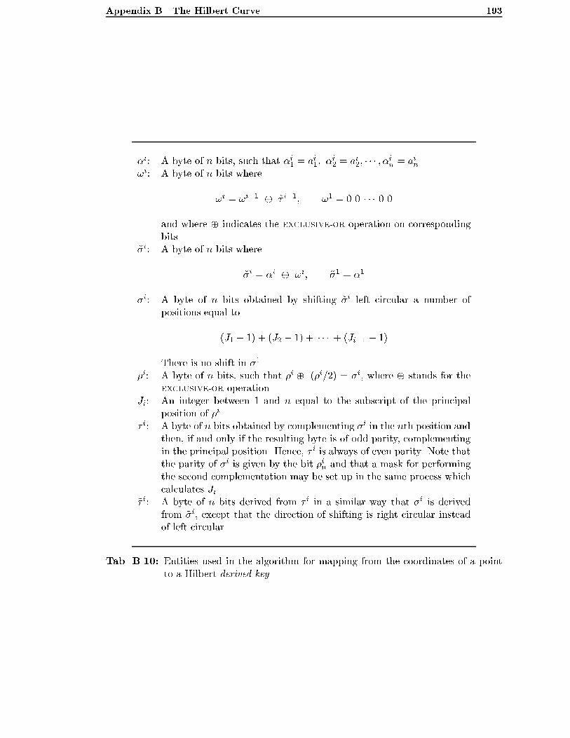
Appendix B. The Hilbert Curve 193
�i: A byte of n bits, such that �i1 = a
i1; �
i2 = a
i2; � � � ; �
in = a
in.
!i: A byte of n bits where
!i = !
i�1 � ~� i�1; !1 = 0 0 � � � 0 0
and where � indicates the EXCLUSIVE-OR operation on corresponding
bits.
~�i: A byte of n bits where
~�i = �i � !
i; ~�1 = �
1
�i: A byte of n bits obtained by shifting ~�i left circular a number of
positions equal to
(J1 � 1) + (J2 � 1) + � � � + (Ji�1 � 1)
There is no shift in �1.
�i: A byte of n bits, such that �i � (�i=2) = �
i, where � stands for the
EXCLUSIVE-OR operation.
Ji: An integer between 1 and n equal to the subscript of the principal
position of �i.
�i: A byte of n bits obtained by complementing �i in the nth position and
then, if and only if the resulting byte is of odd parity, complementing
in the principal position. Hence, � i is always of even parity. Note that
the parity of �i is given by the bit �in and that a mask for performing
the second complementation may be set up in the same process which
calculates Ji.
~� i: A byte of n bits derived from �i in a similar way that �i is derived
from ~�i, except that the direction of shifting is right circular instead
of left circular.
Tab. B.10: Entities used in the algorithm for mapping from the coordinates of a point
to a Hilbert derived-key

194
Appendix C
MOORE'S CURVE: OUR VARIATION
This appendix contains examples of state diagram generator tables for our variation of
Moore's curve in 2 to 4 dimensions. These were produced in accordance with the algo-
rithms given in section 4.3.5.2 in chapter 4.
Y X1 X2 �Y T (Y )
00 00 10 01 0 1
11 -1 0
01 01 10 01 0 1
11 -1 0
10 11 01 01 0 -1
00 1 0
11 10 01 01 0 -1
00 1 0
Tab. C.1: State Diagram Generator Table for our Variation to Moore's Curve in 2 Di-
mensions

Appendix C. Moore's Curve: Our Variation 195
Y X1 X2 �Y T (Y )
000 000 110 001 0 0 1
111 0 -1 0
-1 0 0
001 001 110 001 0 0 1
111 0 -1 0
-1 0 0
010 011 101 001 0 0 -1
100 0 1 0
-1 0 0
011 010 101 001 0 0 -1
100 0 1 0
-1 0 0
100 110 000 001 0 0 1
001 0 1 0
1 0 0
101 111 000 001 0 0 1
001 0 1 0
1 0 0
110 101 011 001 0 0 -1
010 0 -1 0
1 0 0
111 100 011 001 0 0 -1
010 0 -1 0
1 0 0
Tab. C.2: State Diagram Generator Table for our Variation to Moore's Curve in 3 Di-
mensions

Appendix C. Moore's Curve: Our Variation 196
Y X1 X2 �Y T (Y )
0000 0000 1110 0001 0 0 0 1
1111 0 -1 0 0
0 0 -1 0
-1 0 0 0
0001 0001 1110 0001 0 0 0 1
1111 0 -1 0 0
0 0 -1 0
-1 0 0 0
0010 0011 1101 0001 0 0 0 -1
1100 0 -1 0 0
0 0 1 0
-1 0 0 0
0011 0010 1101 0001 0 0 0 -1
1100 0 -1 0 0
0 0 1 0
-1 0 0 0
0100 0110 1000 0001 0 0 0 1
1001 0 1 0 0
0 0 1 0
-1 0 0 0
0101 0111 1000 0001 0 0 0 1
1001 0 1 0 0
0 0 1 0
-1 0 0 0
0110 0101 1011 0001 0 0 0 -1
1010 0 1 0 0
0 0 -1 0
-1 0 0 0
0111 0100 1011 0001 0 0 0 -1
1010 0 1 0 0
0 0 -1 0
-1 0 0 0
Top half of table
Y X1 X2 �Y T (Y )
1000 1100 0010 0001 0 0 0 1
0011 0 1 0 0
0 0 -1 0
1 0 0 0
1001 1101 0010 0001 0 0 0 1
0011 0 1 0 0
0 0 -1 0
1 0 0 0
1010 1111 0001 0001 0 0 0 -1
0000 0 1 0 0
0 0 1 0
1 0 0 0
1011 1110 0001 0001 0 0 0 -1
0000 0 1 0 0
0 0 1 0
1 0 0 0
1100 1010 0100 0001 0 0 0 1
0101 0 -1 0 0
0 0 1 0
1 0 0 0
1101 1011 0100 0001 0 0 0 1
0101 0 -1 0 0
0 0 1 0
1 0 0 0
1110 1001 0111 0001 0 0 0 -1
0110 0 -1 0 0
0 0 -1 0
1 0 0 0
1111 1000 0111 0001 0 0 0 -1
0110 0 -1 0 0
0 0 -1 0
1 0 0 0
Bottom half of table
Tab. C.3: State Diagram Generator Table for our Variation to Moore's Curve in 4 Di-
mensions

197
Appendix D
THE GRAY-CODE CURVE
This appendix relates to mapping to the Gray-code curves we de�ne in chapter 3. In sec-
tion D.1, we show how Bially's [Bia69] state diagram generator table approach, described
in chapter 4, can be adapted to these curves enabling them to be represented by state
diagrams. This is followed in section D.2 with a number of examples of state diagram
generator tables.
D.1 Creation of State Diagram Generator Tables
We identify three of a number of possible curves which use Gray-codes in section 3.7.2 of
chapter 3 and they are referred to as Gray-codeF , Gray-codeA and Gray-codeB .
Means of calculating mappings between Gray-codes and their sequence numbers, or
derived-keys, are relatively simple and are described in chapter 5. In this section, we apply
Bially's state diagram approach to performing mappings to the various Gray-code curves
as an alternative to calculation.
The principal advantage of this lies in the ability to utilize not just the same algorithms
for querying but also the same computer programs, with little or no modi�cation, for the
Gray-code curve as are used for the Hilbert curve. Once constructed, it is a simple matter
to substitute a state diagram for the Hilbert curve with one for the Gray-code curve. This
readily enables the characteristics of the two curves to be explored during experimentation.
In applying Bially's state diagram generation technique to the Gray-code curves, it is
necessary to deviate from the `rules' in populating column X2 of the generator table and
also in populating column X1 in the case of the Gray-codeB curve.
Graphical representations of 2-dimensional Gray-codeF , Gray-codeA and Gray-codeB
curves are shown in chapter 3 in Figures 3.14, 3.16 and 3.18 respectively. Equivalent second
order representations in 3 dimensions are shown in Figures 3.15, 3.17 and 3.19. From these,
generator tables are constructed manually. They are given below in this appendix. These
generator tables provide insights which enable us to develop rules for constructing other
tables for the Gray-code curves in higher-dimensional space, automatically.
Column Y
State diagram generator tables for all three interpretations of the Gray-code curve are
populated in column Y in the same way as the Hilbert curve.
Column X1
Column X1 values follow from the de�nitions of the mappings given in section 3.7.2 of
chapter 3. Thus for the Gray-codeF and Gray-codeA curves they are the Gray-codes of
their corresponding column Y values and for the Gray-codeB curve they are the Gray-code
derived-keys of their corresponding column Y values. ColumnX1 values de�ne `continuous'
Gray-codeF and Gray-codeA �rst order curves but in the case of the Gray-codeB curve a

Appendix D. The Gray-code Curve 198
discontinuity exists between each group of 4 consecutive rows in the table, regardless of
the number of dimensions.
Column X2
We note from the 2 and 3-dimensional examples that in column X2 the number of
di�erent pairs of entries equals half the number of rows in the table in the case of the
Gray-codeF curve. In the case of the Gray-codeA and Gray-codeB curves, the number of
di�erent pairs of entries equals 2.
Algorithms for populating column X2 values in n dimensions are formulated by ex-
tending the sequences which are present in the tables for 2 and 3 dimensions. They are
di�erent for the three interpretations of the Gray-code curve.
Gray-codeF
As with the Hilbert curve and our variation of Moore's curve, we provide examples for
the sequences of orders1 1{3.
Order 1: [ 0; 1; 0; 1 ]
Order 2: [ 00; 10; 11; 01; 11; 01; 00; 10 ]
Order 3: [ 000; 100; 101; 001; 011; 111; 110; 010; 110; 010; 011; 111; 101; 001; 000; 100 ]
Our rules which generate the sequences for order n are given as follows:
1. Append a reflection of the sequence for order n� 1 to the
sequence for order n� 1, thus doubling its size.
2. Divide the members of the enlarged sequence into groups each
containing 4 members.
3. For groups in the first half of the enlarged sequence:
(a) Prefix individual members with a bit taken successively
from the sequence [ 0; 1; 1; 0 ].
(b) If the most significant bit of a member is non-zero then
invert the value of the next lower bit; from 1 to 0 or
from 0 to 1.
4. For groups in the second half of the enlarged sequence:
(a) Prefix individual members with a bit taken successively
from the sequence [ 1; 0; 0; 1 ].
(b) If the most significant bit of a member is zero then
invert the value of the next lower bit; from 1 to 0 or
from 0 to 1.
The sequence of order n is then used to populate the column in the generator table
for n dimensions.
Gray-codeA
In all even numbered rows in the generator table, the �rst column X2 entry equals the
�rst column X1 entry and the second column X2 entry equals the last column X1 entry.
In all odd numbered rows, the same values are used in column X2 except that the last
column X1 entry is used in place of the �rst column X1 entry and vice versa.
1 NB: usage of the term order here is distinct from usage in the context of order of curve

Appendix D. The Gray-code Curve 199
Gray-codeB
In the �rst of the two formats of pairs of column X2 entries, the �rst value of the
pair equals the �rst entry in column X1 and the second value equals the last entry in
column X1. In the second format, the entries are bitwise complements of the �rst format.
We label the formats A and B.
For generator tables in n dimensions, we express the way in which it is determined
whether column X2 in a row should contain a pair of entries of format A or B using the
following rules:
1. For n = 1, initialize column X2 with a pair of entries of
format A followed by a pair of entries of format B.
2. For n > 1:
(a) Copy the sequence of format types in column X2 from the
table for n� 1 dimensions into both the first and second
halves of the column for n dimensions.
(b) In the second half of the table, exchange format A
entries for format B and vice versa.
Column �Y
The column X2 entries cause all of the column �Y entries to equal the last entry in
column X1.
Column T (Y )
Column �Y entries result in the matrices in column T (Y ) being initialized as identity
matrices. The signs of their non-zero elements are adjusted in the way speci�ed by Bially.
D.2 Some Examples of State Diagram Generator Tables
Tables D.1 to D.3 are for the Gray-codeF curve in 2 to 4 dimensions and were produced
in accordance with the algorithms given in section 4.3.5.3 in chapter 4.
Tables D.4 to D.6 are for the Gray-codeA curve in 2 to 4 dimensions and were produced
in accordance with the algorithms given in section 4.3.5.3 in chapter 4.
Tables D.7 to D.9 are for the Gray-codeB curve in 2 to 4 dimensions and were produced
in accordance with the algorithms given in section 4.3.5.3 in chapter 4.

Appendix D. The Gray-code Curve 200
Y X1 X2 �Y T (Y )
00 00 00 10 1 0
10 0 1
01 01 11 10 -1 0
01 0 -1
10 11 11 10 -1 0
01 0 -1
11 10 00 10 1 0
10 0 1
Tab. D.1: State Diagram Generator Table for the Gray-codeF Curve in 2 Dimensions
Y X1 X2 �Y T (Y )
000 000 000 100 1 0 0
100 0 1 0
0 0 1
001 001 101 100 -1 0 0
001 0 1 0
0 0 -1
010 011 011 100 1 0 0
111 0 -1 0
0 0 -1
011 010 110 100 -1 0 0
010 0 -1 0
0 0 1
100 110 110 100 -1 0 0
010 0 -1 0
0 0 1
101 111 011 100 1 0 0
111 0 -1 0
0 0 -1
110 101 101 100 -1 0 0
001 0 1 0
0 0 -1
111 100 000 100 1 0 0
100 0 1 0
0 0 1
Tab. D.2: State Diagram Generator Table for the Gray-codeF Curve in 3 Dimensions

Appendix D. The Gray-code Curve 201
Y X1 X2 �Y T (Y )
0000 0000 0000 1000 1 0 0 0
1000 0 1 0 0
0 0 1 0
0 0 0 1
0001 0001 1001 1000 -1 0 0 0
0001 0 1 0 0
0 0 1 0
0 0 0 -1
0010 0011 0011 1000 1 0 0 0
1011 0 1 0 0
0 0 -1 0
0 0 0 -1
0011 0010 1010 1000 -1 0 0 0
0010 0 1 0 0
0 0 -1 0
0 0 0 1
0100 0110 0110 1000 1 0 0 0
1110 0 -1 0 0
0 0 -1 0
0 0 0 1
0101 0111 1111 1000 -1 0 0 0
0111 0 -1 0 0
0 0 -1 0
0 0 0 -1
0110 0101 0101 1000 1 0 0 0
1101 0 -1 0 0
0 0 1 0
0 0 0 -1
0111 0100 1100 1000 -1 0 0 0
0100 0 -1 0 0
0 0 1 0
0 0 0 1
Top half of table
Y X1 X2 �Y T (Y )
1000 1100 1100 1000 -1 0 0 0
0100 0 -1 0 0
0 0 1 0
0 0 0 1
1001 1101 0101 1000 1 0 0 0
1101 0 -1 0 0
0 0 1 0
0 0 0 -1
1010 1111 1111 1000 -1 0 0 0
0111 0 -1 0 0
0 0 -1 0
0 0 0 -1
1011 1110 0110 1000 1 0 0 0
1110 0 -1 0 0
0 0 -1 0
0 0 0 1
1100 1010 1010 1000 -1 0 0 0
0010 0 1 0 0
0 0 -1 0
0 0 0 1
1101 1011 0011 1000 1 0 0 0
1011 0 1 0 0
0 0 -1 0
0 0 0 -1
1110 1001 1001 1000 -1 0 0 0
0001 0 1 0 0
0 0 1 0
0 0 0 -1
1111 1000 0000 1000 1 0 0 0
1000 0 1 0 0
0 0 1 0
0 0 0 1
Bottom half of table
Tab. D.3: State Diagram Generator Table for the Gray-codeF Curve in 4 Dimensions

Appendix D. The Gray-code Curve 202
Y X1 X2 �Y T (Y )
00 00 00 10 1 0
10 0 1
01 01 10 10 -1 0
00 0 1
10 11 00 10 1 0
10 0 1
11 10 10 10 -1 0
00 0 1
Tab. D.4: State Diagram Generator Table for the Gray-codeA Curve in 2 Dimensions
Y X1 X2 �Y T (Y )
000 000 000 100 1 0 0
100 0 1 0
0 0 1
001 001 100 100 -1 0 0
000 0 1 0
0 0 1
010 011 000 100 1 0 0
100 0 1 0
0 0 1
011 010 100 100 -1 0 0
000 0 1 0
0 0 1
100 110 000 100 1 0 0
100 0 1 0
0 0 1
101 111 100 100 -1 0 0
000 0 1 0
0 0 1
110 101 000 100 1 0 0
100 0 1 0
0 0 1
111 100 100 100 -1 0 0
000 0 1 0
0 0 1
Tab. D.5: State Diagram Generator Table for the Gray-codeA Curve in 3 Dimensions

Appendix D. The Gray-code Curve 203
Y X1 X2 �Y T (Y )
0000 0000 0000 1000 1 0 0 0
1000 0 1 0 0
0 0 1 0
0 0 0 1
0001 0001 1000 1000 -1 0 0 0
0000 0 1 0 0
0 0 1 0
0 0 0 1
0010 0011 0000 1000 1 0 0 0
1000 0 1 0 0
0 0 1 0
0 0 0 1
0011 0010 1000 1000 -1 0 0 0
0000 0 1 0 0
0 0 1 0
0 0 0 1
0100 0110 0000 1000 1 0 0 0
1000 0 1 0 0
0 0 1 0
0 0 0 1
0101 0111 1000 1000 -1 0 0 0
0000 0 1 0 0
0 0 1 0
0 0 0 1
0110 0101 0000 1000 1 0 0 0
1000 0 1 0 0
0 0 1 0
0 0 0 1
0111 0100 1000 1000 -1 0 0 0
0000 0 1 0 0
0 0 1 0
0 0 0 1
Top half of table
Y X1 X2 �Y T (Y )
1000 1100 0000 1000 1 0 0 0
1000 0 1 0 0
0 0 1 0
0 0 0 1
1001 1101 1000 1000 -1 0 0 0
0000 0 1 0 0
0 0 1 0
0 0 0 1
1010 1111 0000 1000 1 0 0 0
1000 0 1 0 0
0 0 1 0
0 0 0 1
1011 1110 1000 1000 -1 0 0 0
0000 0 1 0 0
0 0 1 0
0 0 0 1
1100 1010 0000 1000 1 0 0 0
1000 0 1 0 0
0 0 1 0
0 0 0 1
1101 1011 1000 1000 -1 0 0 0
0000 0 1 0 0
0 0 1 0
0 0 0 1
1110 1001 0000 1000 1 0 0 0
1000 0 1 0 0
0 0 1 0
0 0 0 1
1111 1000 1000 1000 -1 0 0 0
0000 0 1 0 0
0 0 1 0
0 0 0 1
Bottom half of table
Tab. D.6: State Diagram Generator Table for the Gray-codeA Curve in 4 Dimensions

Appendix D. The Gray-code Curve 204
Y X1 X2 �Y T (Y )
00 00 00 10 1 0
10 0 1
01 01 11 10 -1 0
01 0 -1
10 11 11 10 -1 0
01 0 -1
11 10 00 10 1 0
10 0 1
Tab. D.7: State Diagram Generator Table for the Gray-codeB Curve in 2 Dimensions
Y X1 X2 �Y T (Y )
000 000 000 101 1 0 0
101 0 1 0
0 0 1
001 001 111 101 -1 0 0
010 0 -1 0
0 0 -1
010 011 111 101 -1 0 0
010 0 -1 0
0 0 -1
011 010 000 101 1 0 0
101 0 1 0
0 0 1
100 111 111 101 -1 0 0
010 0 -1 0
0 0 -1
101 110 000 101 1 0 0
101 0 1 0
0 0 1
110 100 000 101 1 0 0
101 0 1 0
0 0 1
111 101 111 101 -1 0 0
010 0 -1 0
0 0 -1
Tab. D.8: State Diagram Generator Table for the Gray-codeB Curve in 3 Dimensions

Appendix D. The Gray-code Curve 205
Y X1 X2 �Y T (Y )
0000 0000 0000 1010 1 0 0 0
1010 0 1 0 0
0 0 1 0
0 0 0 1
0001 0001 1111 1010 -1 0 0 0
0101 0 -1 0 0
0 0 -1 0
0 0 0 -1
0010 0011 1111 1010 -1 0 0 0
0101 0 -1 0 0
0 0 -1 0
0 0 0 -1
0011 0010 0000 1010 1 0 0 0
1010 0 1 0 0
0 0 1 0
0 0 0 1
0100 0111 1111 1010 -1 0 0 0
0101 0 -1 0 0
0 0 -1 0
0 0 0 -1
0101 0110 0000 1010 1 0 0 0
1010 0 1 0 0
0 0 1 0
0 0 0 1
0110 0100 0000 1010 1 0 0 0
1010 0 1 0 0
0 0 1 0
0 0 0 1
0111 0101 1111 1010 -1 0 0 0
0101 0 -1 0 0
0 0 -1 0
0 0 0 -1
Top half of table
Y X1 X2 �Y T (Y )
1000 1111 1111 1010 -1 0 0 0
0101 0 -1 0 0
0 0 -1 0
0 0 0 -1
1001 1110 0000 1010 1 0 0 0
1010 0 1 0 0
0 0 1 0
0 0 0 1
1010 1100 0000 1010 1 0 0 0
1010 0 1 0 0
0 0 1 0
0 0 0 1
1011 1101 1111 1010 -1 0 0 0
0101 0 -1 0 0
0 0 -1 0
0 0 0 -1
1100 1000 0000 1010 1 0 0 0
1010 0 1 0 0
0 0 1 0
0 0 0 1
1101 1001 1111 1010 -1 0 0 0
0101 0 -1 0 0
0 0 -1 0
0 0 0 -1
1110 1011 1111 1010 -1 0 0 0
0101 0 -1 0 0
0 0 -1 0
0 0 0 -1
1111 1010 0000 1010 1 0 0 0
1010 0 1 0 0
0 0 1 0
0 0 0 1
Bottom half of table
Tab. D.9: State Diagram Generator Table for the Gray-codeB Curve in 4 Dimensions

206
Appendix E
SOURCE CODE FOR GENERATION OF
STATE DIAGRAMS
The source code required for constructing state diagram generator tables for the Hilbert
curve, our variation of Moore's curve and the Gray-codeF , Gray-codeA and Gray-codeB
curves has been omitted from this version of the thesis.

207
Appendix F
SOURCE CODE FOR DATA MANAGEMENT
IMPLEMENTATION
The source code for the current implementation of our application for the storage, indexing
and retrieval of multi-dimensional data has been omitted from this version of the thesis.

208
Index of de�nitions
approximation, 25
current-page-key, 94
current-page-key-point, 98
current-quadrant, 99
current-query-region, 99
current-search-space, 99
datum-point, 5
derived-key, 5
hyper-cube, 32
hyper-rectangle, 32
n-point, 32
next-match, 93
next-match-point, 98
order of curve, 25
page, 5
page-key, 5
page-key-point, 98
quadrant, 99