the application of pmp for end-point optimization · the application of pmp for end-point...
TRANSCRIPT

The Application of PMP for End-Point Optimization
Srinivas Palanki
University of South Alabama
Srinivas Palanki (USA) The Application of PMP for End-Point Optimization 1 / 33

Outline
1 Motivation
2 Problem Formulation
3 PMP-based Solution Strategy
4 Real-Time Optimization
5 Conclusions
Srinivas Palanki (USA) The Application of PMP for End-Point Optimization 2 / 33
Motivation
Batch Process Applications
The batch mode is used when:
Production volumes are low
Isolation is required
Materials are hard to handle
Flexible plants are desired near markets of consumption
This mode of operation is popular in the pharmaceutical and specialtychemicals industry.
Srinivas Palanki (USA) The Application of PMP for End-Point Optimization 3 / 33
Motivation
Batch Operation
Srinivas Palanki (USA) The Application of PMP for End-Point Optimization 4 / 33

Motivation
Batch Process Characteristics
Inherently dynamic in nature
Nonlinear dynamics
Several batches run in the same equipment
Batch to batch variation in operating conditions
Optimization objective is product quality and quantity at the batchend-point
Srinivas Palanki (USA) The Application of PMP for End-Point Optimization 5 / 33

Motivation
Current Industrial Practice
Development of batch recipe (based on chemistry)
Open-loop implementation of recipe
One end-point measurement for quality
Srinivas Palanki (USA) The Application of PMP for End-Point Optimization 6 / 33

Motivation
Potential for Improvement
Increased computational power at the factory shopfloor
Real-time measurements
Competition from the market
Srinivas Palanki (USA) The Application of PMP for End-Point Optimization 7 / 33
Motivation
Traditional Optimization Approach
Procedure
Develop accurate mathematical model
Solve optimization problem off-line
Implement solution in “open-loop”
Drawbacks
Accurate models take too long to develop
Uncertainties due to differences in lab and industrial equipment
Model parameters not known accurately
Open-loop solution not optimal in the presence of uncertainties
Srinivas Palanki (USA) The Application of PMP for End-Point Optimization 8 / 33
Problem Formulation
Real-Time Optimization Framework
Utilize an approximate model
Compute the optimal operating strategy
Take real-time measurements
Make periodic corrections to the optimal solution during batchoperation to account for uncertainty
Solution strategy should be simple enough that a plant operator canimplement it
Srinivas Palanki (USA) The Application of PMP for End-Point Optimization 9 / 33
Problem Formulation
Process Plant Reality
I do not need your fancy-shmancy algorithm. I can control anything usingmy “PLD” knob.
Anonymous plant operator
Srinivas Palanki (USA) The Application of PMP for End-Point Optimization 10 / 33
Problem Formulation
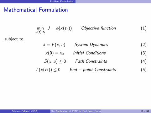
Mathematical Formulation
minu(t),tf
J = φ(x(tf )) Objective function (1)
subject tox = F (x , u) System Dynamics (2)
x(0) = x0 Initial Conditions (3)
S(x , u) ≤ 0 Path Constraints (4)
T (x(tf )) ≤ 0 End − point Constraints (5)
Srinivas Palanki (USA) The Application of PMP for End-Point Optimization 11 / 33
Problem Formulation
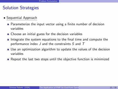
Solution Strategies
• Sequential Approach
Parameterize the input vector using a finite number of decisionvariables
Choose an initial guess for the decision variables
Integrate the system equations to the final time and compute theperformance index J and the constraints S and T
Use an optimization algorithm to update the values of the decisionvariables
Repeat the last two steps until the objective function is minimized
Srinivas Palanki (USA) The Application of PMP for End-Point Optimization 12 / 33
Problem Formulation
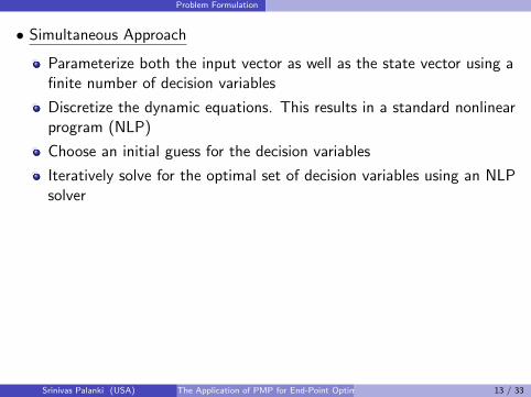
• Simultaneous Approach
Parameterize both the input vector as well as the state vector using afinite number of decision variables
Discretize the dynamic equations. This results in a standard nonlinearprogram (NLP)
Choose an initial guess for the decision variables
Iteratively solve for the optimal set of decision variables using an NLPsolver
Srinivas Palanki (USA) The Application of PMP for End-Point Optimization 13 / 33
Problem Formulation
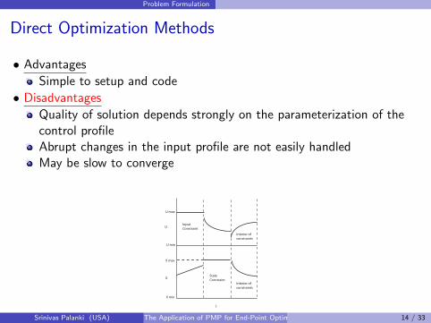
Direct Optimization Methods
• Advantages
Simple to setup and code
• Disadvantages
Quality of solution depends strongly on the parameterization of thecontrol profileAbrupt changes in the input profile are not easily handledMay be slow to converge
U max
U
U min
StateConstraint
X max
X
X min
t
Interior ofconstraints
Interior ofconstraints
InputConstraint
Srinivas Palanki (USA) The Application of PMP for End-Point Optimization 14 / 33

Problem Formulation
PMP Formulation
Equivalent optimization problem:
minu(t),tf
H = λTF (X , u) + µTS(x , u) (6)
subject to
x = F (x , u) x(0) = x0
λT = −∂H
∂xλT (tf ) =
∂φ
∂x|tf + νT ∂T
∂x|tf
µTS = 0νTT = 0
(7)
PMP formulation results in a two point boundary value problem that iscomputationally difficult to solve
Srinivas Palanki (USA) The Application of PMP for End-Point Optimization 15 / 33
PMP-based Solution Strategy
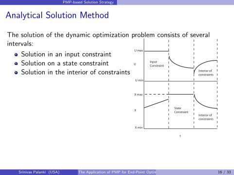
Analytical Solution Method
The solution of the dynamic optimization problem consists of severalintervals:
Solution in an input constraint
Solution on a state constraint
Solution in the interior of constraints
U max
U
U min
StateConstraint
X max
X
X min
t
Interior ofconstraints
Interior ofconstraints
InputConstraint
Srinivas Palanki (USA) The Application of PMP for End-Point Optimization 16 / 33
PMP-based Solution Strategy
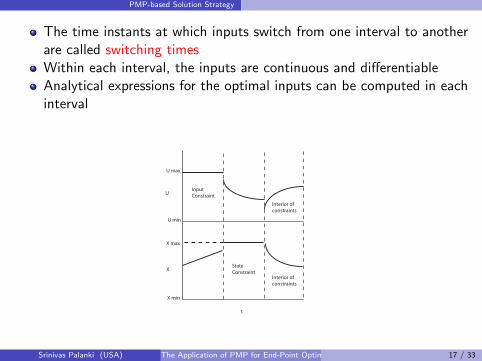
The time instants at which inputs switch from one interval to anotherare called switching timesWithin each interval, the inputs are continuous and differentiableAnalytical expressions for the optimal inputs can be computed in eachinterval
U max
U
U min
StateConstraint
X max
X
X min
t
Interior ofconstraints
Interior ofconstraints
InputConstraint
Srinivas Palanki (USA) The Application of PMP for End-Point Optimization 17 / 33

PMP-based Solution Strategy
PMP Formulation Revisited
minu(t),tf
H(t) = λTF (x , u) + µTS(x , u) (8)
Hui = λTFui + µTSui = 0 (9)
d lHui
dt l= λT ∆lFui − µ
T ∂S
∂x∆l−1Fui = 0 (10)
where ∆ is the Lie Bracket operatorSince the inputs can be (and typically are) affine, Hui and several of itstime derivates are independent of ui .
Srinivas Palanki (USA) The Application of PMP for End-Point Optimization 18 / 33

PMP-based Solution Strategy
Active Path Constraint
Let ζi be the first value of l for which λT ∆lFui 6= 0
A non-zero µ is required to satisfy:
d lHui
dt l= λT ∆lFui − µ
T ∂S
∂x∆l−1Fui = 0 (11)
This implies that at least one of the path constraints is active
Constraint tracking =⇒ regulation problem of relative degree rij = ζi
Srinivas Palanki (USA) The Application of PMP for End-Point Optimization 19 / 33

PMP-based Solution Strategy
Solution Inside the Feasible Region
Let the order of singularity, σi , be the first value of l for which theinput ui appears explicitly and independently in λT ∆lFui
Let ρi be the dimension of the state space that can be reached bymanipulating ui
The optimal input depends on ρi − σi − 1 = ξi adjoint variables
An adjoint-free expression in the feasible region can be obtained from:
Mi =
[Fui
...∆1Fui
...∆2Fui
... . . ....∆ρi−1Fui
... . . .
](12)
where successive Lie brackets are found until the structural rank of Mi
is ρi
I ξi > 0 =⇒ Dynamic State FeedbackI ξi = 0 =⇒ Static State FeedbackI −∞ < ξi < 0 =⇒ System is constrained to a surface
Srinivas Palanki (USA) The Application of PMP for End-Point Optimization 20 / 33
PMP-based Solution Strategy
Parsimonious Parameterization Approach
Choose an initial sequence of intervals
Use analytical expressions for the inputs in each interval
Determine numerically the optimal switching instants
Check the necessary conditions of optimality
If optimality conditions are not satisfied, change the sequence ofintervals and go to step 2
Srinivas Palanki (USA) The Application of PMP for End-Point Optimization 21 / 33
PMP-based Solution Strategy
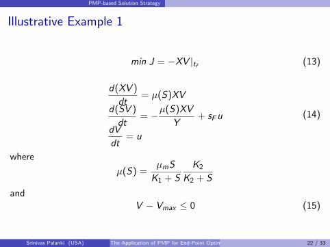
Illustrative Example 1
min J = −XV |tf (13)
d(XV )
dt= µ(S)XV
d(SV )
dt= −µ(S)XV
Y+ sFu
dV
dt= u
(14)
where
µ(S) =µmS
K1 + S
K2
K2 + S
andV − Vmax ≤ 0 (15)
Srinivas Palanki (USA) The Application of PMP for End-Point Optimization 22 / 33
PMP-based Solution Strategy
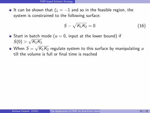
It can be shown that ξ1 = −1 and so in the feasible region, thesystem is constrained to the following surface:
S −√
K1K2 = 0 (16)
Start in batch mode (u = 0, input at the lower bound) ifS(0) >
√K1K2
When S =√
K1K2 regulate system to this surface by manipulating utill the volume is full or final time is reached
Srinivas Palanki (USA) The Application of PMP for End-Point Optimization 23 / 33
PMP-based Solution Strategy
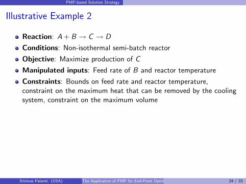
Illustrative Example 2
Reaction: A + B → C → D
Conditions: Non-isothermal semi-batch reactor
Objective: Maximize production of C
Manipulated inputs: Feed rate of B and reactor temperature
Constraints: Bounds on feed rate and reactor temperature,constraint on the maximum heat that can be removed by the coolingsystem, constraint on the maximum volume
Srinivas Palanki (USA) The Application of PMP for End-Point Optimization 24 / 33
PMP-based Solution Strategy
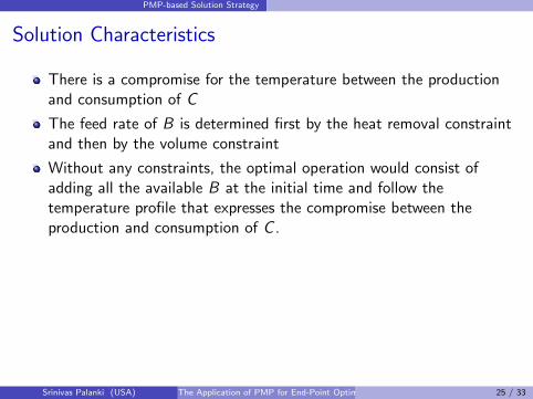
Solution Characteristics
There is a compromise for the temperature between the productionand consumption of C
The feed rate of B is determined first by the heat removal constraintand then by the volume constraint
Without any constraints, the optimal operation would consist ofadding all the available B at the initial time and follow thetemperature profile that expresses the compromise between theproduction and consumption of C .
Srinivas Palanki (USA) The Application of PMP for End-Point Optimization 25 / 33
PMP-based Solution Strategy
Optimal Solution
upath�V
� ((�DH1)k21cAcB(cA � cB) � (�DH2)k2(k1cAcB � k2cC))
(�DH1)k1cA(cBin � cB)
�TV
RT2
((�DH1)E1k1cAcB � (�DH2)E2k2cC)
(�DH1)k1cA(cBin � cB): (81)
6.4.3.2. Analytical expression for Tsens. Tsens is obtained
from the combination of x , u , and T for which the rank
of MT/� [FT DFT D2FT] drops:
F��k1cAcBV
�k2cCV
u
24
35; FT �
V
RT2
E1k1cAcB
E2k2cC
0
24
35;
DFT ��V
RT2
0
k1k2cAcB(E1�E2)
0
24
35� TV
R2T4
�E1k1cAcB(E1�2RT)
E2k2cC(E2�2RT)0
24
35� E1u
RT 2DFu:
The matrix MT has structural rank rT �/2 since the
third element of all involved vector fields is zero.
Intuitively, this is because the temperature cannot affect
the volume. Even though the structural rank is 2, the
rank depends on the states and inputs. The expression
for Tsens can be computed from the determinant of the
first two rows of FT , and DFT . Since FT is already a
function of T , the order of singularity is sT �/0. SincejT �/1, Tsens corresponds to a dynamic feedback:
T sens��RT 2k1cAcB
E2cC
�RT2(cBin � cB)
cB(E1 � E2)
u
V: (82)
The initial condition of Tsens as it enters the sensitivity-
seeking arc is a decision variable, but it can be verifiednumerically that it is equal to Tmax. It is interesting to
note that upath depends on T ; and T sens depends on u .
Thus, if in a given interval u is determined by the path
constraint and T is sensitivity-seeking, then Eqs. (81)and (82) have to be solved simultaneously.
6.4.4. Interpretation of the optimal solution
6.4.4.1. Meeting path objectives. The three arcs of this
solution need to be addressed separately:
. In the first arc, both inputs are on path constraints,
i.e. h�fupath; Tmaxg; and h�fg:/. In the second arc, only the path constraint regarding
the heat production rate is active, for which two
inputs are available. The gain matrix GS : [u , T ]/0/
qrx,max is given by:
(�DH1)k1cA(cBin�cB)½(�DH1)E1k1cAcBV � (�DH2)E2k2cCV
RT 2�
. So, the singular value decomposition of the gain
matrix can be used to compute h and h (see Section
5.2):
h�u (�DH1)k1cA(cBin�cB)
�T(�DH1)E1k1cAcBV � (�DH2)E2k2cCV
RT2;
h�u(�DH1)E1k1cAcBV � (�DH2)E2k2cCV
RT2
�T (�DH1)k1cA(cBin�cB):
. In the third arc, only the input bound for the feed rate
is active. So, h�umin; and h�Tsens:/
6.4.4.2. Meeting terminal objectives. The two switching
times tT and tu parameterize the solution completely.
Since there is only one active terminal constraint,
V (tf)�/Vmax, a combination of the two switching timesis constraint-seeking. The gain matrix, in the neighbor-
hood of the optimum, GT : p0/V (tf)�/Vmax, with p�[tT tu]T; is given by GT � [�0:365 0:268]: The con-
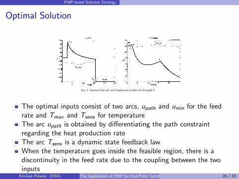
Fig. 4. Optimal feed rate and temperature profiles for Example 4.
B. Srinivasan et al. / Computers and Chemical Engineering 27 (2003) 1�/26 23
The optimal inputs consist of two arcs, upath and umin for the feedrate and Tmax and Tsens for temperatureThe arc upath is obtained by differentiating the path constraintregarding the heat production rateThe arc Tsens is a dynamic state feedback lawWhen the temperature goes inside the feasible region, there is adiscontinuity in the feed rate due to the coupling between the twoinputs
Srinivas Palanki (USA) The Application of PMP for End-Point Optimization 26 / 33
Real-Time Optimization
Presence of Uncertainty
Model MismatchI Available models often do not correspond to industrial reality
F Neglected effects, non-ideal behaviorF Inaccurate parameter values
DisturbancesI Run-to-run variations in initial conditionsI Run-to-run variations in process environment
Srinivas Palanki (USA) The Application of PMP for End-Point Optimization 27 / 33
Real-Time Optimization
Reference Tracking
Determine structure of optimal solution from nominal model
Batch-to-batch update of switching times
Within the batch regulation of active constraints
Tracking sensitivities to nominal trajectories
Real-time optimization problem is reduced to a control problem
Srinivas Palanki (USA) The Application of PMP for End-Point Optimization 28 / 33

Real-Time Optimization
Illustrative Example 3
Reaction:A + B → C rate constant k1
2B → D rate constant k2
Conditions: Semi-batch reactor (feed B), isothermal reactor
Objective: Maximize production of C
Manipulated inputs: Feed rate of B and jacket temperature Tc
Path Constraint: Heat removal limitation (Tc ≥ Tc,min)
Terminal Constraint: Number of moles of D at tf (nDf ≤ nDf ,max)
Uncertainty in k1
Srinivas Palanki (USA) The Application of PMP for End-Point Optimization 29 / 33
Real-Time Optimization
Effect of Uncertainty
The real value of k1 = 0.75 but this is not known to the optimizer.The model can assume values of k1 between 0.4 and 1.2
Solution consists of the flow rate on the upper constraint, switch to aflow rate in the interior of the constraints, and then a switch to thelower constraint
The uncertainty in k1 modifies the values of the switching times, andthe flow rate of B but not the sequence of intervals
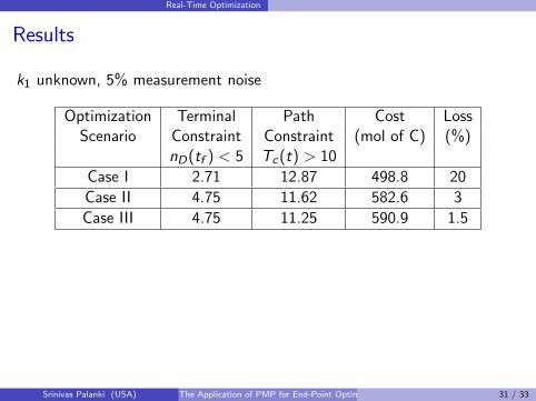
Case I: No measurements are used and an open-loop solution isimplemented
Case II: A measurement of D is made at the end of the batch and theswitching time t2 is adjusted in the subsequent batches
Case III: The temperature, Tc , is measured and the switching time t1and the flow rate of B is adjusted to satisfy the path constraint
Srinivas Palanki (USA) The Application of PMP for End-Point Optimization 30 / 33
Real-Time Optimization
Results
k1 unknown, 5% measurement noise
Optimization Terminal Path Cost LossScenario Constraint Constraint (mol of C) (%)
nD(tf ) < 5 Tc(t) > 10
Case I 2.71 12.87 498.8 20
Case II 4.75 11.62 582.6 3
Case III 4.75 11.25 590.9 1.5
Srinivas Palanki (USA) The Application of PMP for End-Point Optimization 31 / 33

Conclusions
Conclusions
The nominal solution to the dynamic optimization problem can beparameterized efficiently using a PMP formulation
This solution can be utilized in a real-time optimization framework toaccount for uncertainty
Future Work
Model structures for which optimal solution is always on pathconstraints (e.g. linear systems, feedback linearizable systems, flatsystems)
Parameter estimation for batch-to-batch update
Stability results for finite-time processes
Srinivas Palanki (USA) The Application of PMP for End-Point Optimization 32 / 33

Conclusions
..... you control your process using the PLD knob.
Srinivas Palanki (USA) The Application of PMP for End-Point Optimization 33 / 33